financial factors and labour market fluctuations · 2 bank of canada working paper 2011-12 may 2011...
TRANSCRIPT

Working Paper/Document de travail 2011-12
Financial Factors and Labour Market Fluctuations
by Yahong Zhang

2
Bank of Canada Working Paper 2011-12
May 2011
Financial Factors and Labour Market Fluctuations
by
Yahong Zhang
Canadian Economic Analysis Department Bank of Canada
Ottawa, Ontario, Canada K1A 0G9 [email protected]
Bank of Canada working papers are theoretical or empirical works-in-progress on subjects in economics and finance. The views expressed in this paper are those of the author.
No responsibility for them should be attributed to the Bank of Canada.
ISSN 1701-9397 © 2011 Bank of Canada

ii
Acknowledgements
I thank Oleksiy Kryvtsov and Gino Cateau for their helpful suggestions. I have benefited from the discussions from seminar participants at the Bank of Canada, the Annual Meetings of the Canadian Economics Association, Computing in Economics and Finance, and Far-East Econometric Society. I also thank Jill Ainsworth for her research assistance.
iii
Abstract
What are the effects of financial market imperfections on unemployment and vacancies? Since standard DSGE models do not typically model unemployment, they abstract from this issue. In this paper I augment a standard monetary DSGE model with explicit financial and labour market frictions and estimate the model using US data for the period 1964:Q1-2010:Q3. I find that the estimated degree of financial frictions is higher when financial data and shocks are included. The model matches the aggregate volatility in the data reasonably well. In particular, for the labour market, the model is able to generate highly volatile unemployment and vacancies, and a relatively rigid real wage. Further, I find that the financial accelerator mechanism plays an important role in amplifying the effects of financial shocks on unemployment and vacancies. Overall, financial shocks explain about 37 per cent of the fluctuations in unemployment and vacancies.
JEL classification: E32, E44, J6 Bank classification: Economic models; Financial markets; Labour markets
Résumé
Quels effets les imperfections des marchés financiers ont-elles sur le chômage et l’offre d’emplois? Cette question est absente des études qui s’appuient sur les modèles d’équilibre général dynamiques et stochastiques (EGDS) courants, puisque ceux-ci formalisent rarement le phénomène du chômage. L’auteure incorpore des frictions financières et un marché du travail soumis à des frictions dans un modèle monétaire EGDS type, qu’elle estime sur des données américaines s’étalant du 1er trimestre de 1964 au 3e trimestre de 2010. Les frictions financières estimées sont plus intenses lorsque des données et des chocs de nature financière sont ajoutés. Le modèle restitue assez bien la volatilité globale observée dans les données. Plus précisément, la forte volatilité du chômage et de l’offre d’emplois est reproduite, de même que la relative rigidité des salaires réels. L’auteure constate en outre que le mécanisme d’accélérateur financier joue un rôle important car il amplifie l’incidence des chocs financiers sur le chômage et l’offre d’emplois. Dans l’ensemble, ces chocs expliquent environ 37 % des fluctuations du chômage et de l’offre d’emplois.
Classification JEL : E32, E44, J6 Classification de la Banque : Modèles économiques; Marchés financiers; Marchés du travail

1 IntroductionThe recent financial crisis has been associated with a significant rise in the unemployment rate
in the US. The unemployment rate more than doubled from 4.8 per cent at the beginning of the re-cession to peak at 10 per cent in the last quarter of 2009. Determining the extent to which financialmarket imperfections may have contributed to fluctuations in unemployment in the labour marketand the extent to which monetary policy may have helped to alleviate those fluctuations has howeverproved difficult: On the one hand, models that study the effects of financial frictions on unemploy-ment are often too stylized for making quantitative statements. On the other hand, DSGE modelsthat are more suited to quantitative exercises have typically abstracted from modeling the interac-tion between financial imperfection and the labour market. The purpose of this paper is two-fold:(i) First, develop and estimate a quantitative macroeconomic model that incorporates both labourand financial market frictions using US time series data from 1964Q1 to 2010Q3; (ii) Second, ex-plore the interaction of financial and labour market frictions, and assess quantitatively, through thisinteraction, how important it is to consider financial frictions and shocks when addressing labourmarket dynamics.
There is an important strand of literature that studies the effect of financial market imperfectionson unemployment. These studies usually assume that there exists some difficulties for firms toaccess credit and these difficulties affect firms’ hiring decisions. For example, Wasmer and Weil(2004) assume that new entrepreneurs have no wealth of their own and must raise funds in animperfect credit market before they enter the labour market to search for workers. Acemoglu (2001)studies an environment in which an agent decides to become an entrepreneur or a worker. Forentrepreneurs to be able to hire workers, they either need to borrow the necessary funds or use theirown wealth. Both studies show that credit frictions lead to higher unemployment levels. Recentstudies focus more on the effects of credit frictions on the dynamics of unemployment and vacancies.Petrosky-Nadeau (2009) assumes that firms must seek external funds over their net worth to financecurrent vacancies and the credit market is subject to costly state verification type frictions. He showsthat the credit market frictions amplify and propagate the responses of unemployment and vacanciesto productivity shocks. Monacelli, Quadrini and Trigari (2010) study the importance of financialmarkets for unemployment fluctuations, where firms can issue debt under limited enforcement ofdebt contracts. They indicate that in this environment credit shocks can generate large employmentfluctuations.
However, the abovementioned models are stylized models that in most cases only consider theeffects of productivity shocks on unemployment. Without other frictions or competing shocks, itis difficult to quantify the contribution of credit frictions or shocks to labour market fluctuations.DSGE models, in contrast, can allow for many shocks and frictions, and thus are more suited forquantitative exercises. However, although the recent literature in medium-scale DSGE models hasshown a growing interest in the role of financial factors in business cycle fluctuations (Bernanke,Gertler and Gilchrist 1999, herein BGG; and Christiano, Motto and Rostagno 2007), it has largely

abstracted from modeling unemployment in models where financial factors play an important role.One exception is Christiano, Trabandt and Waletin (2007) (herein CTW). CTW introduce BGG-type financial frictions and unemployment into a monetary DSGE model in a small open economysetting, and estimate their model using Swedish data. They find that financial shocks account for 10per cent of the volatility in unemployment in the Swedish economy.
This paper augments a standard DSGE model with financial and labour market frictions alongthe lines of CTW. The financial market frictions are modeled as in BGG. Due to information asym-metry, there are financial frictions in the accumulation and management of capital. BGG have shownthat this type of friction can amplify and propagate shocks to the macroeconomy (financial accelera-tor mechanism). The labour market frictions are modeled in a search and matching framework, andthe wage setting frictions (staggered wage contracting) are modeled as in Gertler, Sala and Trigari(2008) (herein, GST).1 As in CTW, the model economy is also subject to multiple shocks, includingboth productivity and financial shocks. But unlike CTW, this paper focuses on the transmissionmechanism of financial shocks to labour market activities. In particular, this paper highlights theimportant role of the financial accelerator mechanism in amplifying the responses in unemploymentand vacancies to financial shocks. Moreover, this paper attempts to analyze how the interactionbetween financial shocks and wage setting frictions affects labour market outcomes.
In this paper, financial imperfections affect unemployment and vacancies in the following way:After a negative financial shock that reduces the entrepreneurs’ net worth, the worsened balance-sheet position leads entrepreneurs to face a higher risk premium on their external borrowing dueto BGG-type frictions in the financial market. Since the external financing becomes more costly,the demand for capital declines. Given the constant returns to scale aggregate production function,it is optimal for entrepreneurs to keep a constant capital labour ratio. Thus, the demand for labourdeclines as well, leading firms to post fewer vacancies. This reduces the labour market tightness andthe probability for a worker to find a job, leading fewer workers to leave the unemployment state.In this model, the financial accelerator mechanism amplifies the financial shock and generates largefluctuations in unemployment and vacancies even though firms’ vacancy postings are not subject tofinancial frictions directly (spillover effects of the financial factors).
I estimate the model using US data including financial time series data. The main findings ofthe paper are the following. First, the model matches the aggregate volatility in the data reasonablywell. In particular, the model is able to generate highly volatile unemployment and vacancies, anda relatively rigid real wage. Second, the financial wealth shock, the shock affecting net worth inthe entrepreneurs’ sector, accounts for around 37 per cent of the variations of unemployment andvacancies. The financial accelerator mechanism significantly amplifies the effect of the financialwealth shock. Reducing financial frictions by half decreases the contribution of the financial shockto the variations in the key labour market variables by one third. Third, I find that adding financial
1Since the staggered wage contracting in GST (2008) does not have a direct impact on on-going worker employerrelations, it is not vulnerable to the Barro (1977) critique of sticky wages.
2

data into estimation generates a higher value for the elasticity of external finance, the key parametercapturing financial frictions, leading to a larger amplification effect from the financial accelerator.The estimation results without using financial data do not come close to generating the relativevolatility of unemployment and vacancies observed in the data. Lastly, in order to examine thestability of the sample estimates, I divide the data into two subsamples: the first period is from1966:2 -1979:2 (“Great Inflation” period), and the second period is from 1984:1-2010:3, whichcovers the “Great Moderation” period and the recent recession. I find that financial shocks are muchmore persistent and account for a higher portion of variations in unemployment and vacancies inthe US in the second period.
The paper is organized as follows. In the next section, I describe the model, and then go on todiscuss the data and estimation strategy. In Section 4 I present the estimation results and discuss whythe financial shock is important in explaining the variations in the key labour market variables. InSection 5, I discuss several issues regarding the robustness of the results. Finally, section 6 containsconcluding remarks.
2 The ModelIn this section I describe the model economy. I consider an economy populated by a representa-
tive household, retailers, entrepreneurs, capital producers and employment agencies. Each memberin the household consumes, holds nominal bonds, and decides whether to provide labour inelasti-cally to employment agencies. Employment agencies hire workers from a frictional labour market,which is subject to an aggregate matching function. The nominal wage paid to an individual workeris determined by Nash bargaining. However, in each period an employment agency has a fixed prob-ability that it may renegotiate the wage. Employment agencies make hiring decisions and supplylabour services to entrepreneurs at the price of marginal productivity of the labour services. En-trepreneurs also acquire capital from capital producers. Since entrepreneurs have to obtain externalfinance for their capital purchasing, they are subject to financial market frictions. Retailers purchasethe wholesale goods produced by entrepreneurs and differentiate at no cost and sell them to finalgood producers, who aggregate differentiated goods into a homogeneous good and supply it to therepresentative household.
2.1 Households
There is a representative household with a continuum of members of measure one. The number offamily members currently employed is nt. The employed family members earn nominal wage wnt .The unemployed members receive unemployment benefit bt. Each member has the following periodutility function
u(ct) = et log(ct),
3

where ct is consumption of final goods in period t and where et is a preference shock which follows
log et = ρe log et−1 + εet , εet ∼ i.i.d.N(0, σ2εe).
Following Andolfatto (1996) and Merz (1995), I assume that family members are perfectly insuredagainst the risk of being unemployed, thus consumption is the same for each family member. Therepresentative household maximizes lifetime utility
E0
∞∑t=0
βtu(ct). (1)
The wage income from the employed family members is wnt nt, where wnt is determined by Nashbargaining between employment agencies and workers and nt is determined by a search and matchprocess in the labour market. The household also earns income from owning equity in retailers Πt,pays tax Tt and saves by holding a one-period riskless bond Bt. Assuming that the aggregate priceis pt, the representative household is subject to the following budget constraint
ct =wntptnt + bt(1− nt) + Πt − Tt +
Bt − rnt−1Bt−1
pt, (2)
where rnt−1 is the nominal rate of return on the riskless bond.The household maximizes its expected lifetime utility equation (1) subject to equation (2). The
first-order condition for consumption is
etct
1
rnt= βEt
[et+1
ct+1
ptpt+1
].
2.2 Wholesale Firms (Entrepreneurs)
As in BGG, firms are risk-neutral and manage the production of wholesale goods. The productionfunction for wholesale goods is given by
y(j) = f(kt(j), lt(j)) = ωt(j)(kt(j))α(ztlt(j))
1−α.
At the end of period t − 1, entrepreneurs purchase capital kt(j) from capital producers and use itin period t to produce wholesale goods with labour service lt(j), which is supplied by employmentagencies in a competitive labour market. Production is subject to two type of shocks: ωt is theidiosyncratic shock, which is private information to the entrepreneur and is i.i.d across entrepreneursand time, with mean E[ωt(j)] = 1; zt is an exogenous technology shock that is common to all theentrepreneurs, and it follows
log zt = ρz log zt−1 + εzt , εzt ∼ i.i.d.N(0, σ2εz).
4

Capital purchased at the end of period t, kt+1(j), is partly financed from the entrepreneur’s networth, Nt+1(j), and partly from issuing nominal debt, Bt(j):
qtkt+1(j) = Nt+1(j) +Bt(j)
pt, (3)
where qt is the price of capital relative to the aggregate price pt. Note that, unlike in BGG, the debtcontract in this model is in nominal terms. That is, entrepreneurs sign a debt contract that specifiesa nominal interest rate. To ensure that entrepreneurs will never accumulate enough funds to financecapital acquisitions entirely out of net worth, following BGG, I assume that they have finite lives.The probability that an entrepreneur survives until the next period is ηe.
The financial market imperfections are similar to those in BGG: because the idiosyncratic shockωt(j) is private information for the borrowers (entrepreneurs), there exists information asymmetrybetween borrowers and lenders (financial intermediaries). Due to costly state verification, lendershave to pay an auditing cost to observe the output of the borrowers. In BGG the optimal contractis a standard debt with costly bankruptcy: if the entrepreneur does not default, the lender receivesa fixed payment independent of ωt(j) but contingent upon the aggregate state; if the entrepreneurdefaults, the lender audits and seizes the realized return (net of monitoring costs). The risk premiumassociated with external funds, s(.), is defined as the ratio of the entrepreneur’s cost of externalfunds to the cost of internal funds
st =Etr
kt+1
Et
[rnt
ptpt+1
] , (4)
where Etrkt+1 is the expected rate of return of capital (defined in the next section), which is equalto the expected cost of external funds in equilibrium, and Et[rnt
ptpt+1
] is the cost of internal funds.BGG solve a financial contract that maximizes the payoff to the entrepreneur, subject to the lenderearning the required rate of return. BGG shows that this contract implies that the external financepremium, s(.), depends on the entrepreneur’s balance sheet position and it can be characterized by
st = s
(qtkt+1(j)
Nt+1(j)
), (5)
where s′(.) > 0 and s(1) = 1.2 Equation (5) expresses that the external finance premium increaseswith leverage, or decreases with the share of entrepreneurs’ capital investment that is financed by theentrepreneur’s own net worth. This is because when entrepreneurs rely more on external financing,the riskiness of loans increases. Lenders’ expected loss increases and thus they charge a higher riskpremium.
2See Appendix A in BGG for details.
5

2.2.1 Entrepreneurs’ problem
The entrepreneur j’s net worth, wealth accumulated by entrepreneurs from operating the firms, canbe written as
Nt+1(j) = pwt (j)yj + qt(1− δ)kt(j)− pltlt(j)−rnt−1st−11 + πt
bt−1(j), (6)
where pwt is the relative price of wholesale goods, plt is the relative price of labour service whichis provided by employment agencies, and bt is the real debt (bt = Bt/Pt). Thus the net worth isthe entrepreneurs’ earnings: pwt (j)yj + qt(1 − δ)kt(j) net of labour payment pltlt(j) and interestpayments to lenders rnt−1st−1
1+πtbt−1(j). The profit for the entrepreneur j is given by
πt(j) = bt(j) +Nt+1(j)− qtkt+1(j)
= bt(j) + pwt (j)yj − pltlt(j) + qt(1− δ)kt(j)−rnt−1st−11 + πt
bt−1(j)− qtkt+1(j).
The entrepreneur j chooses lt(j), kt+1(j), and bt(j) to maximize
E0
∞∑t=0
βtπt(j).
The first order conditions yields:
lt(j) : pwt∂yt(j)
∂lt(j)= plt, (7)
kt+1(j) : −qt + Etβ[pwt+1
∂yt+1(j)
∂kt+1(j)+ qt+1(1− δ)] = 0, (8)
andbt(j) : 1− Etβ[
rnt st1 + πt+1
] = 0. (9)
Equation (7) shows in the equilibrium the price for labour service is equal to its marginal produc-tivity. Combining equation (8) and (9) yields
Et[pwt+1
∂yt+1(j)∂kt+1(j)
+ qt+1(1− δ)]qt
= Et[rnt st
1 + πt+1
]. (10)
The left hand side of the equation (10) is the expected return of capital, which depends on themarginal productivity of capital pwt+1
∂yt+1(j)∂kt+1(j)
and the capital gain qt+1(1−δ)qt
. The right hand of theequation is the expected cost of external funds, which is a product of risk premium st and theexpected cost of internal funds rnt
1+πt+1. Expected return of capital is defined as
Etrkt+1(j) =
Et[pwt+1(j)
∂yt+1(j)∂kt+1(j)
+ qt+1(1− δ)]qt
. (11)
6

2.2.2 Aggregate Demand for labour Services, Capital and Financial Frictions
In this section I characterize the key equations that describe the aggregate behaviour for the en-trepreneurial sector: equations for the aggregate demand curves for labour and capital, the equationfor the aggregate stock of entrepreneurial net worth. I also address how the financial shock affectsthe demand for labour services in the model.3
Aggregate Demand for labour and CapitalSince production is constant returns to scale, aggregate production is
yt = ktα(ztlt)
1−α.
Aggregating over equation (7) and equation (11) yields the following equations: the aggregatelabour demand equation
pwt (1− α)ytlt
= plt, (12)
and the equation of aggregate expected gross return on capital from periods t to t+ 1
Etrkt+1 =
Et[pwt+1α
yt+1
kt+1+ qt+1(1− δ)]qt
. (13)
Thus, the equilibrium labour services is determined by the demand from the entrepreneurs (equation12) and the supply from the employment agencies; the equilibrium capital demand depends onequation (13) and
Etrkt+1 = str
nt Et
[ptpt+1
], (14)
which is the aggregate supply curve for external financing derived from equation (4).Aggregate Net WorthAggregating over equation (6) yields the aggregate net worth equation
Nt+1 = ηeγt(rkt qt−1kt −
rnt−1st−11 + πt
bt−1).
The aggregate net worth of entrepreneurs at the end of period t, Nt+1, is the sum of equity heldby entrepreneurs surviving from period t − 1. Following Christiano, Motto and Rostagno (2007),I assume that there is a financial wealth shock, an exogenous shock to the survival probability ofentrepreneurs, γt, which follows an AR(1) process:
log γt = ργ log γt−1 + εγt , εγt ∼ i.i.d.N(0, σ2εz).
The reason why the shock on the survival probability of entrepreneurs has effects on their financialwealth is as follows: in the model, the number of entrepreneurs exiting is balanced by the numberthat enter. Since those who exit usually have more net worth than those who enter, when a positive
3See Appendix A for a more detailed derivation for this section’s equations.
7

shock occurs, the aggregate net worth of entrepreneurs increases. This drives down the externalfinance premium, leading entrepreneurs to purchase more capital, which drives up asset price andincreases entrepreneurs’ net worth even more.
Entrepreneurs going out of business will consume their residual equity,
cet = (1− ηe)(rkt qt−1kt −
rnt−1st−11 + πt
(qt−1kt −Nt)
), (15)
where cet is the aggregate consumption of the entrepreneurs who exit in period t.Demand for labour Services and the Financial Shock (spillover effect)As equation (5) suggests, the external finance premium st depends on net worth Nt. After a
positive financial wealth shock (an increase in the survival probability of entrepreneurs), aggregatenet worth increases and the leverage falls. Since the entrepreneurs’ balance-sheet position improves,the external finance premium falls. As a result, the demand for capital increases after a positivefinancial shock. The demand for labour services increases as well after the shock. To understandthis, I rewrite equation (12)
pwt (1− α)ytlt
= plt,
aspwt (1− α)z1−αt (
ktlt
)α = plt. (16)
Equation (16) suggests that given the relative wholesale goods price pwt , the price for labour servicesplt, a constant capital labour ratio kt
ltis optimal for entrepreneurs if the technology shock is absent.
Thus, if a financial shock drives up the demand for capital, it will drive up the demand for labourservices as well.
2.3 Employment Agencies
Following CTW, I assume that the key labour market activities–vacancy postings, wage bargaining–are all carried out by employment agencies instead of entrepreneurs themselves.4 I assume thatentrepreneurs obtain labour services supplied by employment agencies in a competitive labour mar-ket. Each employment agency i supplies labour services nt(i). The labour market is modeled usinga search framework. The employment agencies make vacancy posting decisions and bargain withworkers over nominal wages. I follow GST assuming a staggered multiple period nominal wagecontracting.
In the next subsections, I describe the matching function, employment agencies’ and workers’problem, and wage dynamics under this staggered Nash bargaining mechanism.
4Assuming that entrepreneurs face a frictional labour market will complicate aggregation.
8

2.3.1 Unemployment, Vacancies and Matching
At the beginning of period t, each employment agency i posts vt(i) vacancies in order to attractnew workers and employs nt(i) workers. The total number of vacancies and employed workers arevt =
∫vt(i)di and nt =
∫nt(i)di. The number of unemployed workers at the beginning of period t
isut = 1− nt.
The number of new hires or “matches”, mt, is governed by a standard Cobb-Douglas aggregatematching technology
mt = σmuσt v
1−σt ,
where σm is a parameter governing the matching efficiency. The probability a firm fills a vacancyin period t, qlt, is given by
qlt =mt
vt.
Similarly, the probability that a searching worker finds a job, slt, is given by
slt =mt
ut.
Both firms and workers take qlt and slt as given. In each period, a fraction 1−ρ of existing workforcent exogenously separates from the firms. Thus, the total labour force is the sum of the number ofsurviving workers and the new matches:
nt+1 = ρnt +mt. (17)
2.3.2 Employment Agencies’ Problem
To maximize comparability with the rest of the model, I assume that there are many employmentagencies that supply labour services at a competitive price plt. These agencies combine laboursupplied by households into homogeneous labour services nt =
∫nt(i)di and supply them to en-
trepreneurs. This leaves the equilibrium conditions associated the production of wholesale goodsunaffected even though the labour market is frictional. Define the hiring rate, xt(i), as the ratio ofnew hires, qltvt(i), to the existing workforce, nt(i):
xt(i) =qltvt(i)
nt(i).
Due to the law of large numbers the employment agency knows the likelihood qlt that each vacancywill be filled. The hiring rate is thus the employment agency’s control variable. The total labourforce can be also written as
nt+1 =
∫nt+1(i)di =
∫(ρnt(i) + xt(i)nt(i))di,
9

which gives
mt =
∫xt(i)nt(i)di.
The value of the employment agency Ft(i) is
Ft(i) = pltnt(i)−wnt (i)
ptnt(i)−
κ
2xt(i)
2nt(i) + βEtΛt,t+1Ft+1(i),
where κ2xt(i)
2nt(i) is the quadratic labour adjustment costs of posting vacancies, and βEtΛt,t+1
is the employment agency’s discount rate with Λt,t+1 = ct+1/ct. At any time, the employmentagency chooses the hiring rate xt(i) to maximize Ft(i), given the existing employment stock, nt, theprobability of filling a vacancy, qlt, and the current and expected path of wages, wnt.. Jt(i), the valueto the employment agency of adding another worker at time t, can be obtained by differentiatingFt(i) with respect to nt(i):
Jt(i) = plt −wnt (i)
pt− κ
2xt(i)
2 + (ρ+ xt(i))βEtΛt,t+1Jt+1(i). (18)
The first order condition for vacancy posting equates the marginal cost of adding a worker with thediscounted marginal benefit:
κxt(i) = βEtΛt,t+1Jt+1(i). (19)
Substituting equation (19) into equation (18):
Jt(i) = plt −wnt (i)
pt+κ
2xt(i)
2 + ρβEtΛt,t+1Jt+1(i). (20)
Combining equations yields the following forward looking difference equation for the hiring rate:
κxt(i) = βEtΛt,t+1(plt+1 −
wnt+1(i)
pt+1
+κ
2xt+1(i)
2 + ρκxt+1(i)).
Using the hiring rate condition and the evolution of the workforce, Jt(i) can be written as
Jt(i) = plt −wnt (i)
pt+κ
2xt(i)
2 + ρκxt(i).
2.3.3 Workers’ Problem
The value to a worker of employment at agency i, Vt(i), is,
Vt(i) = wt(i) + βEtΛt,t+1[ρVt+1(i) + (1− ρ)Ut+1].
10

The average value of employment on being a new worker at time t, Vt, is5
Vt = wt + βEtΛt,t+1[ρVt+1 + (1− ρ)Ut+1],
where
Vt =
∫Vt(i)
xt(i)nt(i)
xtntdi.
The value of unemployment, Ut, depends on the unemployment benefit b and the probability ofbeing employed versus unemployed next period:
Ut = b+ βEtΛt,t+1[slt+1Vt+1 + (1− slt+1)Ut+1].
The worker surplus at firm i, Ht(i), and the average worker surplus, Ht, are given by:
Ht(i) = Vt(i)− Ut,
andHt = Vt − Ut.
It follows that:Ht(i) = wt(i)− b+ βEtΛt,t+1[ρHt+1(i)− slt+1Ht+1]. (21)
2.3.4 Nash Bargaining and Wage Dynamics
In this section, I introduce the staggered multi-period wage contracting and describe wage dynamics.A more explicit derivation is provided in Appendix B. Every period, each employment agency hasa fixed probability 1 − λ that it may renegotiate the nominal wage wnt (real wage wt =
wntpt
). Atthe beginning of period t, for employment agencies that are allowed to renegotiate the wage, theynegotiate with the existing workforce, including the new hires. Due to constant returns, all workersare the same at the margin. For employment agencies that are not allowed to renegotiate the wage,all existing and newly hired workers receive the wage paid in the previous period. This simplePoisson adjustment process implies that it is not necessary to keep track of individual firms’ wagehistories, which simplifies aggregation. Given constant returns, all sets of renegotiating employmentagencies and workers at time t face the same problem, and set the same nominal wage, wn∗t . Thus,the renegotiating employment agency i solves the following problem:
maxHt(i)ηJt(i)
1−η,
5See Gertler and Trigari (2009) for details about the average value of employment.
11

s.t.
wnt (i) = wn∗t with probability 1− λ= wnt−1π with probability λ,
where π is the steady-state inflation rate. The first order condition for the Nash bargaining solutionis given by
η∂Ht(i)
∂wnt (i)Jt(i) = (1− η)
∂Jt(i)
∂wnt (i)Ht(i), (22)
with∂Ht(i)
∂wnt (i)= 1/pt + ρλπβEtΛt,t+1
∂Ht+1(i)
∂wnt+1(i),
and∂Jt(i)
∂wnt (i)= −1/pt + ρλπβEtΛt,t+1
∂Jt+1(i)
∂wnt+1(i).
Let εt = pt∂Ht(i)∂wnt (i)
and µt = −pt ∂Jt(i)∂wnt (i)and it can be shown that
εt = µt.
Given this, the first order condition for wages (equation 22) becomes the conventional sharing rule:6
ηJt(i) = (1− η)Ht(i). (23)
However, due to the staggered wage contracting, Jt(i) and Ht(i) are different from the period-by-period Nash bargaining. To examine this, I first use Wt(i) to denote the sum of expected futurewage payments over the existing contract and subsequent contracts
Wt(i) = Et
∞∑s=0
(ρβ)sΛt,t+swt+s(i)
= wt(i) + EtρβΛt,t+1wt+1(i) + Etρ2β2Λt,t+2wt+2(i) + ...,
which can be written as
Wt(i) = ∆tw∗t + (1− λ)Et
∞∑s=1
(ρβ)sEtΛt,t+s∆t+sw∗t+s (24)
where
∆t = Et
∞∑s=0
(ρβλ)sΛt,t+sptpt+s
πs.
6Gertler and Trigari (2009) and Gertler, Sala and Trigari (2008) suggest µt > εt . This means that firms place agreater weight on the future than the workers do since firms have a longer horizon. This horizon effect makes firmsmore patient than workers and thus reduces the workers’ bargaining power. However, it is not the case here.
12

Using Wt(i), Ht(i) and Jr(i) can be written as
Ht(i) = Wt(i)− Et∞∑s=0
(ρβ)sΛt,t+s[b+ st+s+1βΛt+s,t+s+1Ht+s+1],
and
Jt(i) = Et
∞∑s=0
(ρβ)sΛt,t+s[plt+s +
κ
2x2t+s]−Wt(i).
Substituting equation (24) into Ht(i) and Jt(i), we have
Ht(i) = ∆tw∗t − Et
∞∑s=0
(ρβ)sΛt,t+s[b+ st+s+1βΛt+s,t+s+1Ht+s+1 (25)
−(1− λ)(ρβ)Λt+s,t+s+1∆t+s+1w∗t+s+1],
and
Jt(i) = Et
∞∑s=1
(ρβ)sΛt,t+s[plt+s +
κ
2x2t+s(i) (26)
−(1− λ)(ρβ)Λt+s,t+s+1∆t+s+1w∗t+s+1]−∆tw
∗t .
Equations (25) and (26) suggest that with multi-period contracting, Ht(i) and Jt(i) will depend onλ. In the limiting case of λ = 0, Ht(i) and Jt(i) collapse to the values in the conventional period-by-period Nash bargaining. Substituting equations (25) and (26) into the Nash bargaining first-ordercondition,
ηJt(i) = (1− η)Ht(i),
it yields the following equation for the contract wage in real term w∗t :
∆tw∗t = η(pt +
κ
2x2t (i)) + (1− η)(b+ st+1βΛt,t+1Ht+s+1)
+λρβEtΛt,t+1∆t+1w∗t+1. (27)
The first two terms of equation (27) are conventional components for Nash bargaining solutionsfor wages: the first term is the worker’s contribution to the match and the second is the workers’opportunity cost. The third term is from the staggered multi-period contracting. Following Gertlerand Trigari (2009), I define a target wage wtart (i) as the sum of the first two terms:
wtart (i) = η(pt +κ
2x2t (i)) + (1− η)(b+ slt+1βΛt,t+1Ht+s+1).
The target wage is computed as the wage that would arise under period-by-period Nash bargainingfor the employment agency i, taking as given that all other employment agencies and workers op-erates on multi-period wage contracts. It is different from the conventional Nash bargaining wagewflext , which would arise if all employment agencies and workers were operating on period-by-
13

period wage contract:wflext = η(plt +
κ
2x2t + slt+1κxt) + (1− η)b.
To examine the difference, I use the following equation
βEtΛt,t+1Ht+1 =η
1− ηκxt(i) + βEtΛt,t+1λπ
ptpt+1
∆t+1(wt − w∗t ),
and rewrite the target wage equation as
wtart (i) = η(plt +κ
2x2t (i) + κslt+1xt(i)) + (1− η)b
+(1− η)Etslt+1βΛt,t+1λπ
ptpt+1
∆t+1(wt − w∗t )
= η(plt +κ
2x2t + κslt+1xt) + (1− η)b
+η[κ
2(x2t (i)− x2t ) + κslt+1(xt(i)− xt)]
+(1− η)Etslt+1βΛt,t+1λπ
ptpt+1
∆t+1(wt − w∗t ), (28)
where the first term is wflext and wt is the aggregate real wage, which is defined below. As suggestedin Gertler and Trigari (2009), equation (28) reflects the impact of spillovers of economy-wide aver-age wages on the individual bargaining wage between the employment agency and worker. Whenwt exceeds w∗t , everything else equal, it suggests workers’ outside options are good. This will raisethe target wage. The reverse happens if wt is below w∗t . The stickiness in the aggregate wage affectsthe individual wage bargain by this type of spillover, adding more inertia to the individual wages.In addition, the relative hiring rate, xt(i)− xt, can generate spillovers as well.
Finally, the aggregate nominal wage wnt is
wnt = (1− λ)wn∗t + λπwnt−1.
Thus in real terms we havewt = (1− λ)w∗t + λπ
1
πtwt−1.
2.4 Capital Producers
Capital production is assumed to be subject to an investment-specific shock, τt. Capital producerspurchase the final goods from retailers as investment goods, it, and produce efficient investmentgoods, τtit. Efficient investment goods are then combined with the existing capital stock to producenew capital goods, kt+1. The aggregate capital stock evolves according to:
kt+1 = τtit + (1− δ)kt.
14

The shock τt follows the first-order autoregressive process:
log τt = ρx log τt−1 + ετt , ετt ∼ i.i.d.N(0, σ2
ετ ).
Capital producers are also subject to a quadratic capital adjustment cost , ξ2( itkt− δ)2kt. The profit
of capital producers is
Πkt = Et
[qtτtit − it −
ξ
2
(itkt− δ)2
kt
], (29)
and the first-order condition is
Et
[qtτt − 1− ξ
(itkt− δ)]
= 0. (30)
2.5 Retailers
There is a continuum of monopolistically competitive retailers of measure 1. Retailers buy whole-sale goods from entrepreneurs and produce a good of variety j. Let yt(j) be the retail good sold byretailer j to households and let pt(j) be its nominal price. The final good, yt, is the composite ofindividual retail goods,
yt =
[∫ 1
0
yt(j)ε−1ε dj
] εε−1
.
Following the household’s expenditure minimization problem, the corresponding price index, pt, isgiven by
pt =
[∫ 1
0
pt(j)1−εdj
] 11−ε
,
and the demand function faced by each retailer is given by
yt(j) =
(pt(j)
pt
)−εyt. (31)
Following Calvo (1983), each retailer cannot change prices unless it receives a random signal. Theprobability of receiving such a signal is 1 − ν. Thus, in each period, only a fraction of 1 − ν ofretailers reset their prices, while the remaining retailers keep their prices unchanged. Given thedemand function equation (31), the retailer chooses pt(j) to maximize its expected real total profitover the periods during which its prices remain fixed:
EtΣ∞i=0ν∆p
i,t+i
[(pt(j)
pt+i
)yt+i(j)−mct+iyt+i(j)
],
where ∆pt,i ≡ βict+i/ct is the stochastic discount factor and the real marginal cost, mct, is the price
of wholesale goods relative to the price of final goods (pw,t/pt). Let p∗t be the optimal price chosen
15

by all firms adjusting at time t. The first order condition is:
p∗t =
(ε
ε− 1
)Et∑∞
i=0 νi∆p
i,t+imct+1yt+i(1
pt+i)−ε
Et∑∞
i=0 νi∆p
i,t+iyt+i(1
pt+i)1−ε
.
The aggregate price evolves according to:
pt = [νp1−εt−1 + (1− ν)(p∗t )1−ε]
11−ε .
2.6 Government
I assume that the government spending is gt and it balances its budget,
gt = Tt,
where gt follows an AR(1) process,
log gt = (1− ρx) log gss + ρx log gt−1 + εgt , εgt ∼ i.i.d.N(0, σ2
εg).
2.7 Monetary Policy Rules
The central bank is assumed to operate according to the standard Taylor Rule. The central bankadjusts the nominal interest rate, rnt , in response to deviations of inflation, πt, from its steady-statevalue, π, and output, yt, from its steady-state level, y.
rntrn
= (rnt−1rn
)ρr((πtπ
)ρπ(yty
)ρy)1−ρreεmt ,
where rn, π and y are the steady-state values of rnt , πt and yt, and εmt is a monetary policy shockwhich follows
εmt ∼ i.i.d.N(0, σεm).
ρπ, ρy and ρr are policy coefficients chosen by the central bank.
2.8 Aggregation and Equilibrium
The resource constraint for final goods is
ztkαt lt
1−α = ct + cet + it + gt +ξ
2
(itkt− δ)2
kt +κ
2x2tnt.
Furthermore, for the labour market we have
lt = nt.
16

3 Data and Estimation3.1 Data
I first log-linearize the model around the steady-state. Appendix D and E contain the complete log-linear model, as well as the steady-state conditions. I then adopt a Bayesian approach to estimate themodel. I use six series of quarterly US data: output, consumption, investment, nominal interest rate,inflation and external finance cost. The sample spans from 1964Q1 to 2010Q3. Data on output,consumption and investment are expressed in per capita terms using the civilian population aged15 and up. Output is measured by real GDP. Consumption is measured by real expenditures ofnon-durable goods, services and durable goods. Investment is measured by real private investment.The nominal interest rate is measured by Federal Funds rate expressed in quarterly terms. Inflationis the quarter-to-quarter growth rate of the GDP deflator. External finance costs are measured byU.S. business prime lending rate in real terms. All the series are detrended using an HP filter withsmoothing parameter 1600.
Table 1: Calibrated Values
β discount factor 0.99σ inverse of intertemporal substitution of consumption 2α capital share 0.33δ capital depreciation rate 0.025ε intermediate-good elasticity of substitution 11
N/k steady-state ratio of net worth to capital 0.6ηe survivor rate of entrepreneurs 0.985ρ survival rate of firms 0.90sl job finding rate 0.95ql job filling rate 0.75η bargaining power of workers 0.5b parameter for unemployment flow value 0.4σm elasticity in matches to unemployment 0.5
3.2 Calibrated Values
As is standard when taking DSGE models to the data, the parameters for which the data usedcontain only limited information are calibrated to match salient features of the U.S. economy. Table1 reports the calibrated values. There are 13 parameters. Two of them are for financial market, six ofthem are for labour market, and the rest of the parameters are “conventional” parameters. Financialmarket parameters include the survival rate of entrepreneurs, ηe, and the steady-state ratio of networth to capital N/k. I set ηe = 0.985 so that the steady-state external risk premium is 200 basispoints, which is the sample average spread between the prime lending rate and Federal Funds rate.
17

I also set N/k to 0.6, which is close to the value used in Christensen and Dib (2008). In calibration,I adopt the following functional form for the external finance premium:
st =
(qtkt+1
Nt+1
)χ, (32)
where χ is the elasticity of external risk premium with respect to leverage and χ> 0. χ is a “reducedform” parameter capturing financial market frictions.
For the labour market parameters, I set the bargaining power parameter, η, to be 0.5, which iscommonly used in the literature. The elasticity of matches to unemployment, σm, is set to to be 0.5,the midpoint of values typically used. The job separation rate, 1 − ρ, is set to be 0.1, matching theaverage job duration of two and a half years in the US. The job finding rate sl is set to be 0.95 as inShimer (2005). The average job filling rate ql is set to 0.75, which is suggested by den Haan, Rameyand Watson (2000). Following GST, I express b, the steady state flow value of unemployment as
b = b(pl +κ
2x2), (33)
where b is the fraction of the contribution of the worker to the job. I choose b to be 0.4, followingShimer (2005).
I use conventional values for the five ”conventional” parameters. The discount factor β is set tobe 0.99, which corresponds to an annual real interest rate in the steady-state at four per cent. Thecurvature parameter in the utility function, σ, is set to 2, implying an elasticity of intertemporalsubstitution of 0.5. The steady-state depreciation rate, δ, is set to 0.025, which implies an annualrate of depreciation of ten per cent. The parameter of the Cobb-Douglas function, α, is set to be1/3. The steady-state price mark up ε/(ε− 1) is 1.1 by setting ε = 11.
Table 2: Prior and Posterior Distribution of Structural Parameters: Baseline
Prior Posterior distributiondistribution Mode Mean 5% 95%
Risk premium elasticity χ gamma (0.05,0.02) 0.230 0.240 0.203 0.288Calvo wage parameter λ beta (0.67, 0.05) 0.810 0.806 0.777 0.833Calvo price parameter ν beta (0.67, 0.05) 0.538 0.530 0.470 0.590Capital adj. cost parameter ξ norm (0.25, 0.05) 0.217 0.216 0.144 0.292Taylor rule inertia ρr beta (0.75, 0.1) 0.275 0.292 0.213 0.372Taylor rule inflation ρπ gamma(1.5, 0.1) 1.675 1.685 1.562 1.782Taylor rule output gap ρy norm (0.125, 0.15) -0.006 -0.007 -0.022 0.008
18

Table 3: Prior and Posterior Distribution of Shock Parameters: Baseline
Prior Posterior distributiondistribution Mode Mean 5% 95%
Panel A: Autoregressive parametersTechnology ρz beta (0.6,0.2) 0.896 0.891 0.867 0.914Preference ρe beta (0.6,0.2) 0.598 0.591 0.471 0.709Investment ρτ beta (0.6,0.2) 0.834 0.813 0.741 0.882Government ρg beta (0.6,0.2) 0.692 0.687 0.623 0.759Financial ργ beta (0.6,0.2) 0.242 0.270 0.095 0.444Panel B: Standard deviationsTechnology σεz invg (0.005,2) 0.83 0.83 0.76 0.90Monetary σεm invg (0.005,2) 0.34 0.34 0.30 0.38Investment σετ invg (0.005,2) 1.66 1.57 0.98 1.99Preference σεe invg (0.005,2) 1.03 1.06 0.96 1.15Government σεg invg (0.005,2) 1.02 1.02 0.95 1.11Financial σεγ invg (0.005,2) 0.55 0.54 0.41 0.67
3.3 Priors
I estimate the remaining parameters: the elasticity of external risk premium, χ; the capital adjust-ment cost parameter ξ; the Calvo price and wage parameters ν and λ; and the Taylor rule parameters,ρπ, ρy, and ρr. I also estimate the first-order autocorrelations of all the exogenous shocks and theirrespective standard deviations. Tables 2 and 3 report the prior and the posterior distributions foreach of them. Among the behavioural parameters listed in Table 2, the Taylor rule parameters, theCalvo price and capital adjustment cost parameters are rather conventional. For the priors of theseparameters, I closely follow the existing literature. The elasticity of external risk premium χ andCalvo wage parameter λ are less conventional. In the literature, χ is typically calibrated at 0.05 asin BGG. Thus, I assume that χ follows a gamma distribution with mean 0.05 and standard devia-tion 0.02. Since there is not much guidance for the average wage contracting duration, I assumethat Calvo wage parameter λ follows the same prior distribution as Calvo price parameter ν, whichsuggests that firms negotiate wage contract with workers every 3 quarters on average.
The priors of the shock processes are presented in Table 3. I follow Smets and Wouters (2007),the priors on the shock processes are harmonized as much as possible. The standard deviation ofthe shocks are assumed to follow an Inverted Gamma distribution with a mean of 0.5 per cent andtwo degrees of freedom. The persistence of the shock processes is beta distributed with mean 0.6and standard deviation 0.2.
I use Dynare 3.065 to estimate the model and use Metropolis-Hastings algorithm to performsimulations. The total number of draws is 20,000 and the first 20 per cent draws are neglected. Astep size of 0.4 results in a rejection rate of 0.38.
19

4 Estimation Results4.1 Posterior Estimates of the Parameters
Table 2 gives the mode, the mean and the 5 and 95 percentiles of the posterior distribution ofthe behavioral parameters. The risk premium elasticity parameter, χ, is estimated to be around0.24 (mean 0.24, mode 0.23). Christensen and Dib (2008) use maximum likelihood procedure toestimate a sticky-price model with a financial accelerator on U.S. data and suggest that χ is around0.042. Compared to their value, χ = 0.24 is much higher. Since Christensen and Dib (2008)do not use any financial data in their estimation, this much larger elasticity might have resultedfrom the information contained in the financial data I used in the estimation. Calvo wage contractparameter, λ, is estimated to be around 0.81, suggesting a mean of five quarters between wagecontracting periods. This value is higher than the estimate of the same parameter in GST, which isλ = 0.72. This might because the flow value of unemployment, b, of 0.73 used in their paper ismuch higher than the calibrated value of 0.4 in this paper. A higher b helps generate higher volatilityin unemployment and vacancies and lower volatility in real wages. Thus, with a higher b, a lower λis able to generate the same degree of wage rigidity. The estimates of the “conventional” parametersare consistent with other studies. The degree of price stickiness, ν, is estimated to be 0.53, whichimplies average price adjustment duration of half a year. The capital adjustment cost parameter, ξ,is estimated to be around 0.22. For the monetary policy reaction function parameters, ρπ, the Taylorrule inflation parameter, is estimated to be 1.68, and the reaction coefficient to output gap, ρy, isestimated to be -0.007, suggesting that policy respond very little to output gap. There is a relativelylow degree of interest rate smoothing, as the coefficient on the lagged interest rate is estimated to be0.29.
Table 3 presents the estimates of the shock processes. The new shock, financial wealth shock,appears to be the least persistent shock, with an AR(1) coefficient of 0.27. The technology andinvestment shocks are estimated to be most persistent, with a coefficient of 0.89 and 0.81, respec-tively. The mean of the standard error of the shock to investment is 1.57, suggesting it is the mostvolatile shock. In contrast, the standard deviation of the new financial shock is relatively low at0.54.
4.2 Empirical Fit
One way to assess how the model captures the data is to compare the volatilities of the model againstthe data. Table 4 reports this information. Overall the model does a decent job in matching thedata. It does particularly well in matching the volatility in consumption, investment and inflation.For the key labour market variables, the model is able to capture the fact that both unemploymentand vacancies are highly volatile and real wages are relatively rigid, although the model predictedvolatility for each of them is higher than that in the data. For financial variables, the model is ableto capture 50% of the relative volatility in external finance cost fc.
20

Table 4: Relative Standard Deviations: Model vs Data
y c i w v u rn π fcData 1 0.82 5.02 0.44 9.29 8.10 0.28 0.20 0.24Baseline 1 0.83 4.19 0.89 14.00 11.32 0.36 0.23 0.13
4.3 Sources of labour Market Fluctuations
Given the estimation results of the shock processes, I next simulate the model to examine the contri-bution of each shock to the variations in the key labour market variables. Table 5 presents the results.The financial shock appears to be the most important shock determining the variations in unemploy-ment and vacancies. It accounts for 37% of the variations in these two variables. Investment-specificand technology shocks are next in importance, accounting for roughly 33% and 26% of the vari-ations in unemployment and vacancies, respectively. For real wages, the technology shock is themain driving force, and it accounts for 43% of the variations. The financial shock accounts for 30%and investment- specific shock accounts for 23% for the real wages. The result that the financialshock is the main driving force for both unemployment and vacancies is somewhat surprising, giventhat it is the least persistent among the six shocks and has a low standard deviation. This suggeststhat the financial accelerator mechanism might have played an important role in amplifying theshock internally.
Table 5: Variance Decomposition of the Key labour Market Variables
Technology Monetary Financial Investment Preference Governmentu 26.1 1.2 37.2 33.1 0.3 2.0v 26.2 1.3 37.4 32.9 0.3 2.0w 43.7 1.8 29.6 23.4 0.2 1.4
4.4 Amplification Effect of the Financial Accelerator
I examine this issue by simulating the response of several key variables after the financial shock. Ianalyze the role of financial frictions by examining both the baseline model and the same model withthe financial frictions reduced by half (χ is reduced to 0.12).7 Figure 1 illustrates the response ofthe model economy to a negative financial shock. The solid line is the baseline model. The dottedline is the model with χ = 0.12. In both cases, following a negative financial wealth shock, thesurvivor rate of the entrepreneurs decreases, causing the aggregate net worth to fall. This drives upthe external finance premium, forcing entrepreneurs to reduce their demand for capital by reducinginvestment. The fall in demand for capital is accompanied by the fall in demand for labour. Asset
7The rest of the parameters are the same for both models.
21
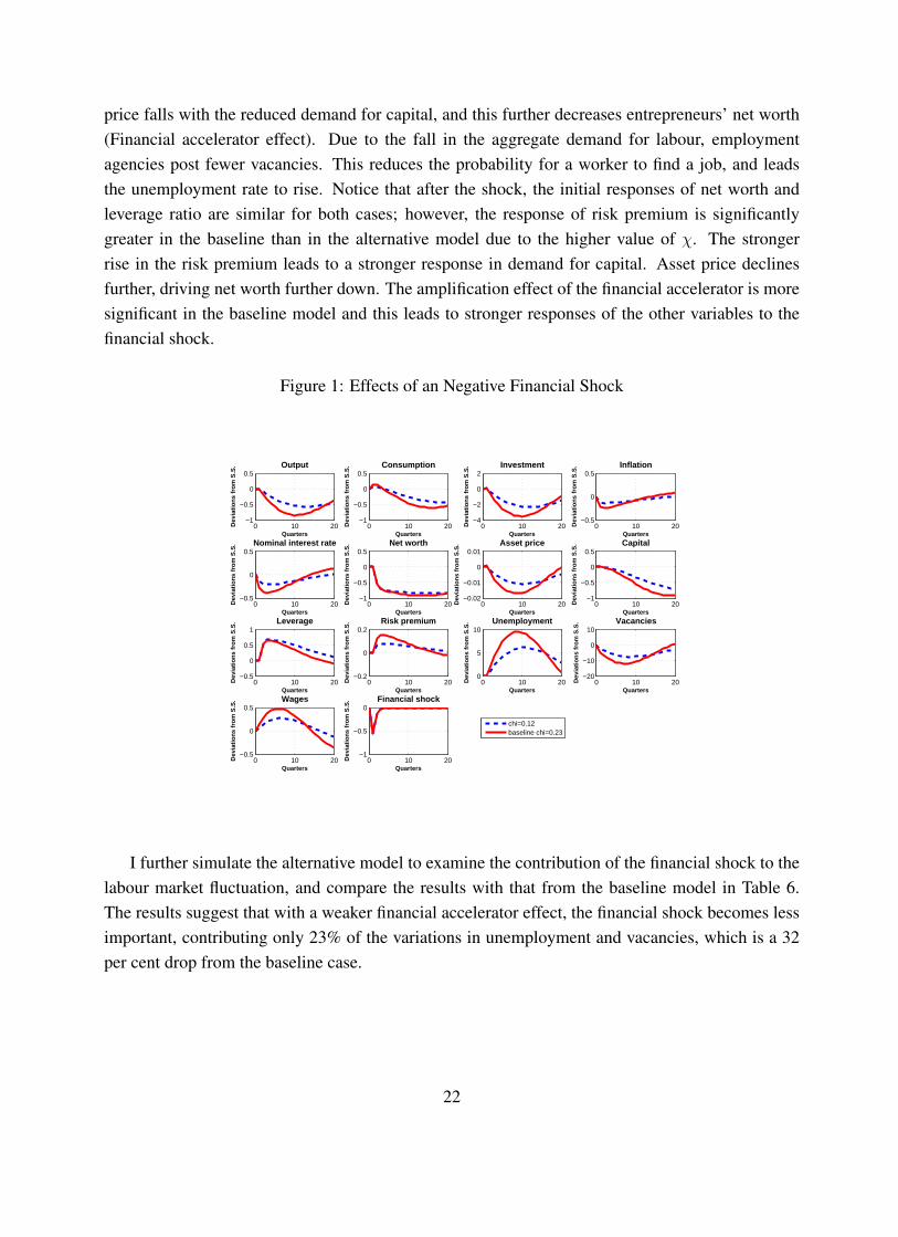
price falls with the reduced demand for capital, and this further decreases entrepreneurs’ net worth(Financial accelerator effect). Due to the fall in the aggregate demand for labour, employmentagencies post fewer vacancies. This reduces the probability for a worker to find a job, and leadsthe unemployment rate to rise. Notice that after the shock, the initial responses of net worth andleverage ratio are similar for both cases; however, the response of risk premium is significantlygreater in the baseline than in the alternative model due to the higher value of χ. The strongerrise in the risk premium leads to a stronger response in demand for capital. Asset price declinesfurther, driving net worth further down. The amplification effect of the financial accelerator is moresignificant in the baseline model and this leads to stronger responses of the other variables to thefinancial shock.
Figure 1: Effects of an Negative Financial Shock
0 10 20−1
−0.5
0
0.5
Quarters
Dev
iati
on
s fr
om
S.S
. Output
chi=0.12baseline chi=0.23
0 10 20−1
−0.5
0
0.5
Quarters
Dev
iati
on
s fr
om
S.S
. Consumption
0 10 20−4
−2
0
2
Quarters
Dev
iati
on
s fr
om
S.S
. Investment
0 10 20−0.5
0
0.5
Quarters
Dev
iati
on
s fr
om
S.S
. Inflation
0 10 20−0.5
0
0.5
Quarters
Dev
iati
on
s fr
om
S.S
. Nominal interest rate
0 10 20−1
−0.5
0
0.5
Quarters
Dev
iati
on
s fr
om
S.S
. Net worth
0 10 20−0.02
−0.01
0
0.01
Quarters
Dev
iati
on
s fr
om
S.S
. Asset price
0 10 20−1
−0.5
0
0.5
Quarters
Dev
iati
on
s fr
om
S.S
. Capital
0 10 20−0.5
0
0.5
1
Quarters
Dev
iati
on
s fr
om
S.S
. Leverage
0 10 20−0.2
0
0.2
Quarters
Dev
iati
on
s fr
om
S.S
. Risk premium
0 10 200
5
10
Quarters
Dev
iati
on
s fr
om
S.S
. Unemployment
0 10 20−20
−10
0
10
Quarters
Dev
iati
on
s fr
om
S.S
. Vacancies
0 10 20−0.5
0
0.5
Quarters
Dev
iati
on
s fr
om
S.S
. Wages
0 10 20−1
−0.5
0
Quarters
Dev
iati
on
s fr
om
S.S
. Financial shock
I further simulate the alternative model to examine the contribution of the financial shock to thelabour market fluctuation, and compare the results with that from the baseline model in Table 6.The results suggest that with a weaker financial accelerator effect, the financial shock becomes lessimportant, contributing only 23% of the variations in unemployment and vacancies, which is a 32per cent drop from the baseline case.
22

Table 6: Variance Decomposition for labour Market Variables: a Comparison
Less friction (χ = 0.12) BaselineShocks Unemployment Vacancy Real wage Unemployment Vacancy Real wageTechnology 33.04 33.19 49.46 25.97 26.06 43.54Monetary 1.39 1.45 1.75 1.24 1.3 1.77Investment 40.15 40.06 28.84 32.99 32.71 23.27Preference 0.24 0.23 0.16 0.3 0.3 0.22Government 1.57 1.56 1.07 1.97 1.96 1.37Financial 23.6 23.52 18.71 37.51 37.67 29.82
4.5 Financial shock and financial data
In order to further identify the importance of the financial shock and financial data, I re-estimate themodel but without the financial shock and without the financial time series. I compare the resultsfrom the alternative model (NoFS model) with the baseline model in Tables 7 and 8. The estimatesof the behavioral parameters and the shock processes do not change much. There is, however,a large change in the estimate of the elasticity of external financing: χ falls to 0.009 from 0.23.This significant change might reflect the fact that it is important to include financial time series toidentify financial frictions. I next explore how well the NoFS model is able to account for the
Table 7: Posterior Mode of Structural Parameters: No FS vs. Baseline
PosteriorNoFS Baseline
Mode SD Mode SDRisk premium elasticity χ 0.009 0.004 0.230 0.023Calvo wage parameter λ 0.628 0.039 0.810 0.014Calvo price parameter ν 0.703 0.054 0.538 0.038Capital adj. cost parameter ξ 0.230 0.050 0.217 0.050Taylor rule inertia ρr 0.238 0.047 0.275 0.046Taylor rule inflation ρπ 1.841 0.086 1.675 0.062Taylor rule output gap ρy 0.021 0.015 -0.006 0.009
overall volatility in the data compared to the baseline model. Table 9 presents the results. Overall,NoFS model matches the data less well. In particular, the NoFS model does not come close togenerating the relative volatility of unemployment and vacancies in the data. Table 10 presents thecomparison of the variance decomposition of the key labour market variables for the two models.Without the financial shock, the technology shock becomes the most important shock: it explains78% of the variance of unemployment and vacancies, and 96% of the variance of real wage.
23
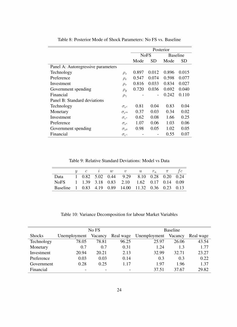
Table 8: Posterior Mode of Shock Parameters: No FS vs. Baseline
PosteriorNoFS Baseline
Mode SD Mode SDPanel A: Autoregressive parametersTechnology ρz 0.897 0.012 0.896 0.015Preference ρe 0.547 0.074 0.598 0.077Investment ρτ 0.816 0.033 0.834 0.027Government spending ρg 0.720 0.036 0.692 0.040Financial ργ - - 0.242 0.110Panel B: Standard deviationsTechnology σεz 0.81 0.04 0.83 0.04Monetary σεm 0.37 0.03 0.34 0.02Investment σετ 0.62 0.08 1.66 0.25Preference σεe 1.07 0.06 1.03 0.06Government spending σεg 0.98 0.05 1.02 0.05Financial σεγ - - 0.55 0.07
Table 9: Relative Standard Deviations: Model vs Data
y c i w v u rn π fcData 1 0.82 5.02 0.44 9.29 8.10 0.28 0.20 0.24NoFS 1 1.39 3.18 0.83 2.10 1.62 0.17 0.14 0.09Baseline 1 0.83 4.19 0.89 14.00 11.32 0.36 0.23 0.13
Table 10: Variance Decomposition for labour Market Variables
No FS BaselineShocks Unemployment Vacancy Real wage Unemployment Vacancy Real wageTechnology 78.05 78.81 96.25 25.97 26.06 43.54Monetary 0.7 0.7 0.31 1.24 1.3 1.77Investment 20.94 20.21 2.13 32.99 32.71 23.27Preference 0.03 0.03 0.14 0.3 0.3 0.22Government 0.28 0.25 1.17 1.97 1.96 1.37Financial - - - 37.51 37.67 29.82
24

5 IssuesIn this section I address several issues involving the robustness of the results.
5.1 Staggered wage contracting
The previous section suggests that without the significant amplification effect from the financialaccelerator mechanism (χ = 0.009), staggered wage contracting alone cannot generate enoughvolatility in unemployment and vacancies. This result seems to contradict the finding in GST that amodel with wage rigidity provides a better fit for the dynamics of the labour market variables. Theirresults do not rely on the amplification effect of the financial accelerator. However, as noticed inthe previous section, the flow value of unemployment in GST, b, is much higher. As suggested inHagedorn and Manovskii (2008), when b is close to unity, the value of unemployment is very closeto that of employment to the worker. Since labour supply is very elastic in this case, this high bmight have helped their model to capture unemployment and wage dynamics in the data. Moreover,the workers’ bargaining power parameter, η, used in GST, is 0.9, which lies well above the rangeconsidered in the literature, 0.5-0.7. In order to examine the effects of these “unconventional” valueson the labour market dynamics, I simulate the model using their values for b and η while keepingthe rest of the parameters the same as in the NoFS case
Table 11: Relative Standard Deviations: Model Comparison
y c i w v u rn π fcData 1 0.82 5.02 0.44 9.29 8.10 0.28 0.20 0.24Baseline 1 0.83 4.19 0.89 14.00 11.32 0.36 0.23 0.13NoFS 1 1.39 3.18 0.83 2.10 1.62 0.17 0.14 0.09No FS with high b and η 1 0.53 4.59 0.80 13.14 10.38 0.15 0.10 0.08Baseline w/ flexible wages 1 1.97 3.40 0.88 1.79 1.45 0.46 0.29 0.21
Table 11 shows that with the higher values for the flow value of unemployment and bargainingpower, the NoFS model generates similar variability in unemployment and vacancies as the baselinemodel, suggesting that mechanically these unconventional values play the same role in amplifyingthe responses in unemployment and vacancies to shocks as the financial accelerator mechanism inthe baseline model.
Although the staggered wage contracting is not a sufficient condition to generate enough vari-ability in unemployment and vacancies, it is a necessary condition for the model in this paper tomatch the data. To examine how important this type of wage setting friction is in the model, I sim-ulate the baseline model again but assume period-by-period wage contracting (by setting λ = 0),and compare the relative volatilities of the key variables generated by the alternative model (the lastrow in Table 11) with the baseline case. As Table 11 makes clear, the flexible wage case is not ableto generate enough variability in unemployment and vacancies even though the external finance
25

premium stays very elastic (χ = 0.23). This result confirms the argument of recent studies that theconventional search models cannot account for the key cyclical movements of unemployment andvacancies in the labour market.
Overall, Table 11 suggests that the interaction of the financial accelerator mechanism and wagesetting frictions is the key for the model to match the data.
5.2 Elasticity of External Risk Premium
The elasticity of the external risk premium χ is the key parameter of the financial accelerator mecha-nism. In BGG, χ is a “reduced form” parameter that captures financial frictions. It is determined bythe “deep” parameters in the original BGG model: the variance of idiosyncratic shocks to the returnon capital, the bankruptcy costs, and entrepreneurs’ survival rate. In the literature, it is typicallycalibrated at 0.05.8 The examples of estimated models based on BGG for US data are Christensenand Dib (2008), De Graeve (2008) and Queijo (2009). None of these paper use financial data.Christensen and Dib (2008) and Queijo (2009) estimate χ to be around 0.04.9 De Graeve (2008)estimates χ to be at 0.1. Compared to these values, the estimate of χ = 0.23 in the baseline modelis substantially higher. As suggested in the previous section, the high value of χ might be due tothe inclusion of the financial data. In other words, the non financial variables used in the estimationin those studies contain very limited information on financial frictions, thus χ is underestimated.Another example is CTW. CTW estimate a model with financial shocks and use two financial timeseries. They have not estimated χ explicitly, however, the estimated monitoring cost parameter intheir model, which is one of “deep” parameters determining χ, is almost 4 times higher than the oneBGG proposed.10
5.3 Estimations of Subsamples
Since the importance of the financial shock depends χ and χ can be sensitive to the sample period,I follow Smets and Wouters (2007) and divide the data into two subsamples: the first one is the“Great Inflation” period 1966:2-1979:2, and the second subsample is from 1984:1-2010:3, whichincludes mostly the “Great Moderation” period and the recent recession. I estimate the modelover these two subsamples. It is well-known that output and inflation volatility fall considerablyduring the “Great Moderation” period. Table 12 presents the standard deviations of the key macro
8See for examples, Bernanke, Gertler and Gilchrist (1999) and Bernanke and Gertler (2000).9Queijo (2009) does not estimate χ directly; instead she estimates parameters for bankruptcy costs and survival rate
of entrepreneurs. The estimates of these parameters imply that χ is 0.04.10The estimated value of χ = 0.009 in the NoFS case is lower than conventional wisdom. To investigate why χ
is low in the NoFS model. I re-estimate the NoFS model using the data from the same time period from 1979Q3 to2004Q3 as Christensen and Dib (2008). I also reset the quarterly survival rate for entrepreneurs, ηe, to be the value of0.9728 used in their paper in order to capture the fact that during this period the average spread is higher. The estimateof χ is around 0.02, which is closer to the estimated value in Christensen and Dib (2008), although it is still lower. Thissuggests that the difference in sample periods might be one factor contributing the difference in the estimation results.
26

variables and the key labour market variables. It shows that the volatilities of the unemploymentand vacancies fall as well, although the volatility in real wage appears to stay the same. Table 13
Table 12: Standard Deviations of Subsamples
66:1-79:2 84:1-10:3Output 0.016 0.010Consumption 0.014 0.008Investment 0.076 0.058Real wage 0.005 0.005Vacancy 0.138 0.112Unemployment 0.132 0.103Nom. Interest rate 0.005 0.003Inflation 0.004 0.002
compares the modes of the posterior distribution of the model parameters over these two periods.Similar to Smets and Wouters (2007), the most significant differences between the two subsamplesare in the variances of the shock processes. The standard deviations of all the shocks considered inthe model fall in the second period, including the financial shock, which falls by half from 0.56 to0.23. The persistence of these shocks changes much less for the most part; however, interestinglythe persistence of the financial shock increases significantly during the second period from 0.29 to0.62. Table 14 shows that due to this increased persistence, the financial shock accounts for a higherportion of the variability in unemployment, vacancies and real wages.11
6 Concluding RemarksIn this paper, I argue that the spillover effects of financial market shocks are important for
labour market fluctuations. Although the estimation results suggest that the financial disturbanceis neither persistent nor volatile, the financial accelerator mechanism amplifies the financial shockand generates large fluctuations in the labour market. Overall, I find that more than 30 per centof the variations in unemployment and vacancies is explained by the financial shock. I show thatignoring these financial shocks and financial data can reduce the model’s explanatory power. Inparticular, the model without these financial factors has difficulties matching the observed volatilityin unemployment and vacancies.
However, the fit of the model largely relies on the value of one key parameter: χ, the parameterthat summarizes the frictions in the financial market. I show that the estimate of χ lies aboveconventional wisdom when the financial data is included in the estimation. To ensure that thiskey parameter is well identified, more work on checking the robustness of the model is necessary.Another line of future research would be to incorporate financial frictions that explicitly affect firms’
11I have also estimated the model for the “Great Moderation” period only (1984:1-2004:4). The results are similarto those from the second subsample. This might be due to that the recent recession period is relatively short, and the“Great Moderation” periods dominate the results for the second subsample.
27

Table 13: Subsample Estimates
Structural parameters Shock process1966:1-1979:2 1984:1-2010:3 1966:1-1979:2 1984:1-2010:3Mode SD Mode SD Mode SD Mode SD
χ 0.206 0.0296 0.2139 0.0203 ρz 0.9039 0.0267 0.8491 0.0263λ 0.7704 0.0312 0.8107 0.0162 ρe 0.5499 0.1531 0.6645 0.073ν 0.5778 0.0412 0.5678 0.0406 ρτ 0.8668 0.0317 0.8553 0.022ξ 0.2383 0.05 0.2202 0.0502 ρg 0.6944 0.0768 0.6253 0.0568ρr 0.317 0.0658 0.4976 0.0554 ργ 0.29 0.1716 0.6203 0.1085ρπ 1.5068 0.0822 1.8207 0.0839 σεz 0.99 0.09 0.56 0.04ρy 0.017 0.0208 -0.0165 0.0146 σεm 0.35 0.04 0.2 0.02
σετ 2.16 0.47 1.54 0.22σεe 1.39 0.17 0.83 0.06σεg 1.12 0.11 0.91 0.06σεγ 0.56 0.11 0.23 0.04
Table 14: Variance Decomposition: Subsamples
1966:1-1979:2 1984:1-2010:3Unemployment Vacancy Real wage Unemployment Vacancy Real wage
Technology 30.56 30.6 58.76 13.71 13.89 25.72Monetary 1.32 1.41 1.73 1.82 1.9 2.84Investment 33.05 32.65 17.56 41.97 41.62 33Preference 0.4 0.4 0.21 0.44 0.44 0.36Government 2.09 2.09 1.02 1.86 1.86 1.56Financial 32.58 32.86 20.71 40.2 40.3 36.52
28

hiring decisions into a monetary DSGE model. As the existing literature has already shown, firms’hiring activities can be directly related to how easily firms are able to access external funds. Itwould be interesting to evaluate the impact of this type of financial frictions on unemployment andvacancies at the aggregate level.
29

7 Appendix7.1 Appendix A: Aggregation of labour and Capital Demand, Aggregation
of Net Worth
For each entrepreneur j, the labour demand is determined by
∂yt(j)
∂lht (j)= (1− α)
yt(j)
lt(j)= plt.
Since all the firm j has the same output labour ratio, aggregating this first order condition yields
pwt (1− α)ytlt
= plt.
Define the expected return on capital as
Etrkt+1(j) =
Et[pwt+1(j)α
∂yt+1(j)∂kt+1(j)
+ qt+1(1− δ)]qt
,
and aggregate over this first order condition, we have
EtRkt+1 =
∫ Et[pwt+1(j)α
∂yt+1(j)∂kt+1(j)
+ qt+1(1− δ)]qt
dj
=Et[p
wt+1(j)α
∂yt+1
∂kt+1+ qt+1(1− δ)]
qt.
The entrepreneur j’s net worth is given by
Nt+1(j) = pwt (j)yj − pltlt(j) + qt(1− δ)kt(j)−rnt−1st−11 + πt
bt−1(j),
which can be written as
nt+1(j) = pwt (j)yt(j)− pltlt(j)−rnt−1st−1(j)
1 + πtbt−1(j) + qt(1− δ)kt(j)
= pwt (j)yt(j)− pwt (1− α)yt(j)
lt(j)lt(j)−
rnt−1st−1(j)
1 + πtbt−1(j) + qt(1− δ)kt(j)
= pwt αyt(j)
kt(j)kt(j)−
rnt−1st−1(j)
1 + πtbt−1(j) + qt(1− δ)kt(j)
=[pwt α
yt(j)kt(j)
+ qt(1− δ)]qt−1
qt−1kt(j)−rnt−1st−1(j)
1 + πtbt−1(j).
30

Given that rkt (j) =[pwt α
yt(j)kt(j)
+qt(1−δ)]qt−1
, the aggregate net worth is
nt+1 = η(rkt qt−1kt −rnt−1st−11 + πt
bt−1).
7.2 Appendix B: Contract Wage7.2.1 Period-by-period Nash Bargaining Contract Wage
For standard period-by-period Nash bargaining, the first order condition is12
ηJt = (1− η)Ht.
This implies that the bargaining wage is
wt =wntpt
= η(plt +κ
2x2t + ρβEtΛt,t+1Jt+1) (34)
+(1− η)(b− βEtΛt,t+1(ρ− st+1)Ht+1).
Substituting the following two equations
κxt = βEtΛt,t+1Jt+1,
andHt+1 =
ηJt+1
1− η,
into equation (34) gives the period-by-period wage wflext as
wflext = wt =wntpt
= η(plt +κ
2x2t + slt+1κxt) + (1− η)b.
7.2.2 Solving for Staggered Wage Contract
First Order Condition for Wage Now turning to the staggered wage contract. The first ordercondition with respect to wnt (i) is
η∂Ht(i)
∂wnt (i)Jt(i) = (1− η)
∂Jt(i)
∂wnt (i)Ht, (35)
where∂Ht(i)
∂wnt (i)= 1/pt + ρλπβEtΛt,t+1
∂Ht+1(i)
∂wnt+1(i),
12Since it is period-by-period Nash bargaining, there is no need to have subscript i to indicate for the firm thatrenegotiate wages in the current period.
31

and∂Jt(i)
∂wnt (i)= −1/pt + ρλπβEtΛt,t+1
∂Jt+1(i)
∂wnt+1(i).
Define
εt = pt∂Ht(i)
∂wnt (i),
and we haveεt = 1 + ρλβπEtΛt,t+1
ptpt+1
εt+1,
with the steady-state εssεss =
1
1− ρλβπ.
Define
µt = −pt∂Jt(i)
∂wnt (i),
and we haveµt = 1 + ρλβπEtΛt,t+1
ptpt+1
µt+1,
with the steady-state µssµss =
1
1− ρλβπ.
Thus,εt = µt
Derivation of Ht(i) and Jt(i) Define
Wt(i) = Et
∞∑s=0
(ρβ)sΛt,t+swt+s(i)
= wt(i) + Etwt+1(i) + Etwt+2(i) + ... (36)
Considering a renegotiating firm i at time t, we have
wt(i) =wn∗tpt,
Etwt+1(i) = Et1
pt+1
[λπwn∗t + (1− λ)wn∗t+1],
32

Etwt+2(i) = Et1
pt+2
[λπwn∗t+1 + (1− λ)wn∗t+2]
= Et1
pt+2
[λπ(λπwn∗t + (1− λ)wn∗t+1) + (1− λ)wn∗t+2]
= Et1
pt+2
[λ2π2wn∗t + λ(1− λ)πwn∗t+1 + (1− λ)wn∗t+2],
and so on. Substituting the above equations into equation (36), we can write Wt(i) as
Wt(i) =wn∗tpt
+ρβEtΛt,t+11
pt+1
[λπwn∗t + (1− λ)wn∗t+1]
+(ρβ)2EtΛt,t+2Et1
pt+2
[λ2π2wn∗t + λ(1− λ)πwn∗t+1 + (1− λ)wn∗t+2]
+...,
that is
Wt(i) = w∗t
+ρβEtΛt,t+1[λπptpt+1
w∗t + (1− λ)w∗t+1]
+(ρβ)2EtΛt,t+2Et[λ2π2 pt
pt+2
w∗t + λ(1− λ)πpt+1
pt+2
w∗t+1 + (1− λ)w∗t+2]
+....
Combining terms, we have
Wt(i) = [1 + ρβλΛt,t+1ptpt+1
π + (ρβλ)2Λt,t+2ptpt+2
π2 + ...]w∗t
+ρβ(1− λ)EtΛt,t+1[1 + ρβλΛt+1,t+2pt+1
pt+2
π]w∗t+1
+....
Define
∆t = Et
∞∑s=0
(ρβλ)sΛt,t+sptpt+s
πs,
where∆ss =
1
1− ρβλ.
33

We can show that
Wt(i) = ∆tw∗t + (1− λ)ρβEtΛt,t+1∆t+1w
∗t+1
+(1− λ)(ρβ)2EtΛt,t+2∆t+2w∗t+2
+...,
that is
Wt(i) = ∆tw∗t + (1− λ)Et
∞∑s=1
(ρβ)sEtΛt,t+s∆t+sw∗t+s. (37)
For Ht(i) we have
Ht(i) = wt(i)− b+ βEtΛt,t+1[ρHt+1(i)− slt+1Ht+1]
= wt(i)− b− slt+1βEtΛt,t+1Ht+1 + ρβEtΛt,t+1Ht+1(i)
= wt(i)− b− slt+1βEtΛt,t+1Ht+1
+ρβEtΛt,t+1[wt+1(i)− b+ βEt+1Λt+1,t+2[ρHt+2(i)− slt+2Ht+2]]
= wt(i) + ρβEtΛt,t+1wt+1(i)− b− ρβEtΛt,t+1b
−slt+1βEtΛt,t+1Ht+1 − ρβEtΛt,t+1βEt+1Λt+1,t+2slt+2Ht+2
+(ρβ)2EtΛt,t+2[wt+2(i)− b+βEt+2Λt+2,t+3[ρHt+3(i)− slt+3Ht+3]].
Combining terms,
Ht(i) = Wt(i)− Et∞∑s=0
(ρβ)sΛt,t+s[b+ slt+sβΛt+s,t+s+1Ht+s+1].
Substituting equation (37) into the above equation, we obtain
Ht(i) = ∆tw∗t + (1− λ)Et
∞∑s=1
(ρβ)sEtΛt,t+s∆t+sw∗t+s
−Et∞∑s=0
(ρβ)sΛt,t+s[b+ slt+s+1βΛt+s,t+s+1Ht+s+1] (38)
34

For the value of job Jt(i) , we have
Jt(i) = plt − wt(i) +κ
2x2t (i) + ρβEtΛt,t+1Jt+1(i)
= plt − wt(i) +κ
2x2t (i)
+ρβEtΛt,t+1[plt+1 − wt+1(i)
+κ
2x2t+1(i) + ρβEt+1Λt+1,t+2Jt+2(i)]
= plt + ρβEtΛt,t+1plt+1 +
κ
2x2t (i)
+ρβEtΛt,t+1κ
2x2t+1(i)− wt(i)
−ρβEtΛt,t+1wt+1(i)
+ρβEtΛt,t+1ρβΛt+1,t+2Jt+2(i) + .... (39)
Substituting Wt(i) into equation (39), we obtain
Jt(i) = Et
∞∑s=0
ρsβsΛt,t+s[plt+s +
κ
2x2t+s(i)]−W J
t (i)
= Et
∞∑s=0
ρsβsΛt,t+s[plt+s +
κ
2x2t+s(i)]
−∆tw∗t − (1− λ)Et
∞∑s=1
ρsβsEtΛt,t+s∆t+sw∗t+s (40)
Nash Bargaining Solution under Staggered Nominal Wage Contracting Substituting equation(38) and (40) into Nash bargaining first-order condition
ηJt(i) = (1− η)Ht(i),
we can have
∆tw∗t
= Et
∞∑s=0
(ρβ)sΛt,t+s{η(plt+s +κ
2x2t+s(i)) + (1− η)(b+ st+s+1βΛt+s,t+s+1Ht+s+1)}
−Et∞∑s=1
(1− λ)(ρβ)sΛt,t+s∆t+sw∗t+s.
35

That is,
∆tw∗t
= Et
∞∑s=0
(ρβ)sΛt,t+s{η(plt+s +κ
2x2t+s(i)) + (1− η)(b+ st+s+1βΛt+s,t+s+1Ht+s+1)
−(1− λ)ρβΛt+s,t+s+1∆t+s+1w∗t+s+1},
which can be written in a recursive form as
∆tw∗t = η(plt +
κ
2x2t (i)) + (1− η)(b+ st+1βΛt,t+1Ht+1)
−(1− λ)ρβΛt,t+1∆t+1w∗t+1
+ρβEtΛt,t+1∆t+1w∗t+1.
Thus, the contract wage w∗t equation is
∆tw∗t = η(plt +
κ
2x2t (i)) + (1− η)(b+ st+1βΛt,t+1Ht+1)
+λρβΛt,t+1∆t+1w∗t+1.
The aggregate wage wnt can be written as
wnt = (1− λ)wn∗t + λπwnt−1,
i.e.ptwt = (1− λ)ptw
∗t + λπpt−1wt−1.
Thus in real terms we havewt = (1− λ)w∗t + λπ
1
πtwt−1.
Now we replace Ht+1 in the target wage equation with relative hiring rate (xt(i) − xt) andrelative wage (wt − w∗t ). Given that
Ht(i) = Wt(i)− Et∞∑s=0
(ρβ)sΛt,t+s[b+ slt+s+1βΛt+s,t+s+1Ht+s+1],
36

we have
Et[Ht+1 −Ht+1(i)] = Et[Wt+1 −Wt+1(i)]
= Et
∞∑s=0
(ρβ)sΛt+1,t+s+1(wt+s+1 − wt+s+1(i))
= Et{λπptpt+1
(wt − w∗t ) + ρβΛt+1,t+2λ2π2 pt
pt+2
(wt − w∗t )
+(ρβ)2Λt+1,t+3λ3π3 pt
pt+3
(wt − w∗t ) + ...}
= Et{λπptpt+1
(1 + ρβΛt+1,t+2λπpt+1
pt+2
+ (ρβ)2Λt+1,t+3(λπ)2pt+1
pt+3
+ ...)(wt − w∗t )}
= λπptpt+1
[Et
∞∑s=0
(ρβλ)sΛt+1,t+1+spt+1
pt+1+s
πs](wt − w∗t )
= λπptpt+1
∆t+1(wt − w∗t ).
Recall
∆t = Et
∞∑s=0
(ρβλ)sΛt,t+sptpt+s
πs,
and we also useEt(wt+1 − wt+1(i)) = Etλπ
ptpt+1
(wt − w∗t ),
Et(wt+2 − wt+2(i)) = Etλ2π2 pt
pt+2
(wt − w∗t ),
...,
in the derivation of the above equation. We can then write the first order condition of Nash bargain-ing as
ηtEtJt+1(i) = (1− ηt)EtHt+1(i)
= (1− ηt)(EtHt+1 − λπptpt+1
∆t+1(wt − w∗t )).
Rewrite the above equation as
EtHt+1 =ηEtJt+1(i)
1− η+ Etλπ
ptpt+1
∆t+1(wt − w∗t ).
Given thatκxt(i) = βEtΛt,t+1Jt+1(i), (41)
we haveβEtΛt,t+1Ht+1 =
η
1− ηκxt(i) + βEtΛt,t+1λπ
ptpt+1
∆t+1(wt − w∗t ).
37

Now the target wage can be expressed in terms of (wt − w∗t ) and (xt(i)− xt)
wtart (i) = η(plt +κ
2x2t (i)) + (1− η)(b+ Ets
lt+1βΛt,t+1Ht+1)
= η(plt +κ
2x2t (i) + κslt+1xt(i)) + (1− η)b
+(1− η)Etslt+1βΛt,t+1λπ
ptpt+1
∆t+1(wt − w∗t )
= η(plt +κ
2x2t + κslt+1xt) + (1− η)b
+η[κ
2(x2t (i)− x2t ) + κslt+1(xt(i)− xt)]
+(1− η)Etslt+1βΛt,t+1λπ
ptpt+1
∆t+1(wt − w∗t ).
If we definewflext = η(plt +
κ
2x2t + κsltxt) + (1− η)b,
then the targeted wage can be further written as
wtart (i) = wflext + η[κ
2(x2t (i)− x2t ) + κslt+1(xt(i)− xt)]
+(1− η)slt+1βΛt,t+1λπptpt+1
∆t+1(wt − w∗t ).
7.3 Appendix C: System of Equationsu′(etct)
pt= βrnt
u′(et+1ct+1)
pt+1
Etrkt+1 =
Et[pwt+1α
yt+1
kt+1+ qt+1(1− δ)]qt
Etrkt+1 = Et
rnt st1 + πt+1
Nt+1 = ηeγt[rkt qt−1kt −
rnt−1st−11 + πt
(qt−1kt −Nt)]
st = (qtkt+1
Nt+1
)χ
kt+1 = (1− δ)kt + τtit
qtτt = 1 + ξ(itkt− δ)
mt = uσt v1−σt
nt+1 = ρnt +mt
ut = 1− nt
38

xt =qltvtnt
κxt(i) = βEtΛt,t+1[plt+1a−
wnt+1(i)
pt+1
+κ
2xt+1(i)
2 + ρκxt+1(i)]
wflext = η(plt +κ
2x2t + κslt+1xt) + (1− η)b
wtart (i) = wflext + η[κ
2(x2t (i)− x2t ) + κslt+1(xt(i)− xt)]
+(1− η)slt+1βΛt,t+1λπptpt+1
∆t+1(wt − w∗t )
∆tw∗t = wtart (i) + λρβEtΛt,t+1∆t+1w
∗t+1
∆t = 1 + EtΛt,t+1(ρλβ)ptpt+1
π∆t+1
wnt = (1− λ)wn∗t + λπwnt−1
pwt (1− α)ytlt
= plt
yt = ct + cet + it + gt +κ
2x2tnt +
ξ
2(itkt− δ)2kt
yt = ztkαt l
1−αt
p∗t =
(ε
ε− 1
)Et∑∞
i=0 νi∆i,t+imct+1yt+i(
1pt+i
)−ε
Et∑∞
i=0 νi∆i,t+iyt+i(
1pt+i
)1−ε
pt = [νp1−εt−1 + (1− ν)(p∗t )1−ε]
11−ε .
rntrn
= (rnt−1rn
)ρr((πtπ
)ρπ(yty
)ρy)1−ρreεmt ,
7.4 Appendix D: Log-linearized System of Equations
λt = rt + λt+1 − Etπt+1
λt = uc + et
EtRkt+1 =
mcα yk
mcα yk
+ q(1− δ)(mct+1 + yt+1 − kt+1) +
(1− δ)mcα y
k+ q(1− δ)
qt+1 − qt
EtRkt+1 = rt + st − Etπt+1
nwt+1 =k
NRkt − (
k
N− 1)(rt−1 + st−1 − πt) + nwt + γt
st = χ(qt + kt+1 − nt+1)
kt+1 = (1− δ)kt + δıt + δτt
39

qt = ξδ(ıt − kt)− τt
mt = σut + (1− σ)vt
nt = ρnt + (1− ρ)mt
ut = −nunt
xt = qlt + vt − nwt
xt = EtΛt,t+1 + (β
κx)(pEtp
lt+1 − wEtwt+1) + β(x+ ρ)Etxt+1
wflext =ηpl
wplt +
ηκx(x+ s)
wxt +
ηκxs
wslt
wtart = wflext + (τ1 + τ2)(wt − w∗t )
w∗t = (1− ρβλ)wflext + ρβλEtw∗t+1 + (1− ρβλ)(τ1 + τ2)(wt − w∗t ) +
ρβλ
1− ρβλEtπt+1
where τ1 = η(x+ sl)λβ 11−(x+ρ)λβ and τ2 = (1− η)slβ λ
1−ρβλ
wt = (1− λ)w∗t + λ(wt−1 − πt)
plt = mct + yt − lt
yt =c
yct +
i
yıt +
g
ygt +
κx2n
y(xt +
nt2
)
yt = zt + αkt + (1− α)lt
rnt = ρrrnt−1 + (1− ρr)(ρππt + ρyyt) + εrt
7.5 Appendix E: Steady-state Calculations
π = 1
mc =ε− 1
ε
rn =π
β
rk =1
ηe
s =rk
rn/π
q = 1
i = δk
y
k=rk − (1− δ)
αmc
40

l
k= (
y
k)−(1/1−α)
y
l=y
k/l
k
pl = (1− α)mcy
l
n =sl
1− ρ+ sl
u = 1− n
x = slu/n
x(i) = x
m = slu
v =m
ql
σm =m
uσv1−σ
κ and w are solved from the following two steady-state conditions
κx = β(pl − w +κ
2x2 + ρκx)
w = η(pl +κ
2x2 + slκx) + (1− η)b
whereb = b/(pl +
κ
2x2)
wflex = wtar = w∗ = w
l = n
y =y
ll
k = l/(l/k)
N = k(N/k)
i = (i/k)k
c = y − i− (κ
2)x2n
λ = 1/c
X =λmcy
1− νpβπε
Y =λy
1− νpβπε−1
41

p∗ = (1− νppε−1
1− νp)1/(1−ε)
42

References[1] Acemoglu, D., 2001. “Credit Market Imperfections and Persistent Unemployment,” European
Economic Review 45, 665-679
[2] Andolfatto, D. 1996. “Business Cycles and labour Market Search,” American Economic Re-view 86, 112-132
[3] Barro, R. 1977. “Long-Term Contracting, Sticky Prices and Monetary Policy,” Journal of Mon-etary Economics, 3(3), 305-16
[4] Bernanke, B., M. Gertler and S. Gilchrist. 1999. “The Financial Accelerator in a QuantitativeBusiness Cycle Framework,” Handbook of Macroeconomics, 1341-93
[5] Bernanke, B. and M, Gertler. 2000. “Monetary Policy and Asset Price Volatility,” NBER Work-ing paper No. 7559
[6] Calvo, Guillermo. 1983, “Staggered Prices in a Utility Maximizing Framework,” Journal ofMonetary Economics, 12:383-98
[7] Christensen, Ian and Ali, Dib. 2008. “The Financial Accelerator in an Estimated New Keyne-sian Model,” Review of Economic Dynamics 11, 155-178
[8] Christiano, L., M. Trabandt, and K. Waletin. 2007. “Introducing Financial Frictions and Un-employment into a Small Open Economy Model,” Sveriges Riksbank Working Paper Series214, November 2007
[9] Christiano, L., R. Motto, and M. Rostagno. 2007. “Financial Factors in Business Cycles,”November 2007
[10] Christiano, L., M. Eichenbaum, and C., Evans. 2005. “Nominal Rigidities and the DynamicEffects of a Shock to Monetary Policy,” Journal of Political Economy, 113(1): 1-45
[11] De Graeve, Ferre. 2008. “The External Finance Premium and the Macroeconomy: US post-WWII Evidence,” Journal of Economic Dynamics and Control 32, 3415-40
[12] Den Haan, Wouter J, Garey Ramey, and Joel Watson. 2000. “Job Destruction and Propagationof Shocks.” American Economic Review, Vol. 90, pp. 482-98
[13] Gertler, M., and A. Trigari. 2009. “Unemployment Fluctuations with Staggered Nash WageBargaining,” Journal of Political Economy, Vol. 117, No. 1, pp. 38-86
[14] Gertler, M., L. Sala and A. Trigari. 2008. “An Estimated Monetary DSGE Model with Unem-ployment and Staggered Nominal Wage Bargaining ” Journal of Money, Credit and Banking,Vol. 40, No.8, 1714-64
43

[15] Hagedorn, Macus, and Iourri Manovskii. 2008. “The Cyclical behaviour of Equilibrium Un-employment and Vacancies Revisited.” American Economic Review 98(4), 1692-1706
[16] Merz, M. 1995. “Search in the labour Market and the Real Business Cycles,” Journal of Mon-etary Economics 36, 269-300
[17] Monacelli, T., Quadrini V., and A., Trigari. 2010. “Financial Markets and Unemployment,”Unpublished manuscript
[18] Petrosky-Nadeau, N. 2009. “Credit, Vacancies and Unemployment Fluctuations,” Unpublishedmanuscript, Carnegie Mellon University
[19] Queijo von Heideken, V. 2009, “How Important are Financial Frictions in the United Statesand the Euro Area?,” Scandinavian Journal of Economics, Vol 111(3), 567-96
[20] Shimer, R. 2005. “The Cyclical behaviour of Equilibrium Unemployment, Vacancies, andWages: Evidence and Theory,” American Economic Review 95(1), 25-49
[21] Smets, F and R. Wouters. 2007. “Shocks and Frictions in US Business Cycles: A BayesianDSGE Approach,” American Economic Review 97(3), 586-606
[22] Wasmer, E. and P. Weil. 2004. “The Macroeconomics of labour and Credit Market Imperfec-tions,” American Economic Review 94(4), 944-963
44