Financial Globalization, Home Equity Bias and InternationalRisk-Sharing

Gianluca Benigno�y

Federal Reserve Bank of New York, London School of Economics, CEP

and CEPR

Hande Küçük-Tu¼ger

London School of Economics, CEP

July 2008

Abstract

Recent empirical evidence suggests that the massive wave of �nancial globalization has beenaccompanied by a decline in home equity bias and changes in international risk-sharing. Theobjective of this paper is to reconcile these facts in a theoretical framework. By increasingthe number of assets that can be traded internationally we show that even if home equitybias is somehow reduced, international risk sharing is still above the one observed in the data.Explaining the linkages between �nancial globalization, home equity bias and international risk-sharing is still a challenge for current model of international portfolio allocation.

JEL Classi�cation: F31, F41

Keywords: Portfolio choice, incomplete �nancial markets, international risk sharing, port-

folio choice, �nancial integration.

�Address: Gianluca Benigno, Department of Economics and CEP, London School of Economics and PoliticalScience, Houghton Street, London, WC2A 2AE, United Kingdom. E-mail: g.benigno@lse.ac.uk

yWe would like to thank our discussant Viktoria Hnatkovska and the participants at the IMF Macro-FinanceConference 24-25 April Washington.

1

Manuscript

1 Introduction

The last two decades have witnessed a dramatic increase in international capital �ows. Lane and

Milesi Ferretti (2001, 2006) have documented the increase in gross holdings of cross-country bond

and equities for various countries. This unparalleled expansion in private international asset trade

has largely been a developed-country phenomenon, but developing countries have also participated.

Lane and Milesi-Ferretti (2006) shows indeed that gross external �nancial positions now exceed

100% of GDP for major industrialized countries.

This massive wave of �nancial globalization has been accompanied by changes in international

portfolio in bonds and equities and changes in international risk sharing. Indeed, Sorensen et

al (2007) document the implications of �nancial integration for international portfolio allocation

and international risk sharing by examining OECD countries during the period 1993-2003. Their

empirical analysis shows that �nancial globalization has been accompanied by a decline in home

bias in debt and equity holdings with a corresponding increase in international risk-sharing. On

average they �nd that from 1993 to 2003 and for the countries in their sample, the value of foreign

equity holdings as a percentage of GDP increased from 0.09 to 0.31, the value of foreign debt

holdings increased from 0.47 to 1.2 and a similar pattern arises for the value of equity and debt

liabilities (from 0.1 to 0.37 for equities and 0.67 to 1.35 for debt). Their measures of international

risk-sharing displays a related pattern: income risk sharing and consumption risk sharing increased

quite steeply through the 1990s. Moreover their empirical analysis suggest that declining home

bias has been associated with strongly increasing consumption risk sharing, where the e¤ect is

mostly due to an decline in equity home bias rather than debt home bias. In short the main

conclusion from Sorensen et al (2007) is that home bias and international risk sharing are closely

related phenomena. Obstfeld (2007) on the other hand measures the degree of risk-sharing by

looking at averages of consumption growth and real exchange rates for various country as in the

original Backus and Smith (1993) paper: using this metric there is a distinct negative relationship

(i.e. faster consumption growth is associated with a real appreciation) in the data for the period

going from 1991 to 2006 (the period of �nancial integration) suggesting a worsening rather than an

2

improvement in international risk-sharing.

Is it possible to reconcile in a common framework the aforementioned stylized facts about inter-

national capital markets? That is, can we generate less home bias through �nancial globalization

and what are the consequences of �nancial integration for international risk-sharing?

To address theoretically these questions, we construct a general equilibrium model with two

countries (Home and Foreign) and two sectors (tradable and nontradable) where each country is

specialized in its own tradable good: this model encompasses most of the current models that have

been used in recent international portfolio allocation analysis1. In order to capture di¤erent stages

of �nancial market integration we solve the model under various �nancial market con�gurations

(see also Devereux and Sutherland, 2006b), di¤erent in the number of assets that are traded across

countries going from the simple bonds economy to the case in which we allow trade in all equities

and bonds. At most in our economy agents can trade equities in tradable, nontradable sectors and

Home and Foreign nominal bonds. We allow for shocks to tradables and nontradables endowments

and redistributive shocks to tradable and non-tradable income as to make the international asset

structure incomplete.

Our model is driven mainly by supply shocks: in general following a positive supply shocks the

real exchange rate depreciate and in order to share risk domestic agents will hold foreign assets to

hedge against domestic income risks. In our model by introducing non-traded goods we allow for

the possibility that, depending on the origin of the supply shock (i.e. traded versus non traded), the

real exchange rate and relative consumption across countries can move in opposite directions (see

Benigno and Thoenissen, 2007) so that home assets bias in our model could result as an implication

of the lack of international risk sharing. This feature of the model though depends critically on the

type of assets that are traded internationally: when only real bonds are traded internationally, risk

sharing is limited and the comovements between real exchange rate and consumption induce agents

to short home bonds (compatible with the evidence as in Coeurdacier and Gourinchas, 2008). The

opposite result holds once we consider nominal bonds: risk sharing becomes perfect and agent go

1Our analysis is restricted, though, to a �exible price economy. Engel and Matsumoto (2007, 2008) and Devereuxand Sutherland (2006b) consider models with sticky prices.

3

long on home bonds. As we allow for equities to be traded (either only tradable equities or both

tradable and non-tradable equities) we �nd that home equity bias declines as risk sharing improves

but quantitatively the correlation between consumption and real exchange rate is well above the

one observed in the data. Moreover the possibility of trading nominal bonds along with equities

generates once again perfect risk-sharing and a strong home equity bias.

In short the main result of our analysis is that explaining simultaneously the decline in home eq-

uity bias with the size of international risk-sharing as economies become more �nancially integrated

constitutes still a serious challenge for international portfolio models.

In the next section we brie�y review the related literature. Section 3 describes the model set-

up. Section 4 describes the parametrization and Section 5 analyzes the implications of the di¤erent

asset market structures.

2 Related Literature

Our work is related to several papers in di¤erent ways. On the role of non-tradeability in addressing

the home equity bias, Stockman and Dellas (1989) made an earlier contribution to solve for the

optimal portfolio with nontraded goods. They study an endowment economy with separable utility

between nontraded and traded goods. Their optimal equity portfolio is a combination of a well

diversi�ed portfolio in traded good sector equities and a complete home bias portfolio in nontraded

good sector equities. In another contribution Baxter, Jermann and King (1998) study portfolio

allocation in an endowment economy and assume perfect substitutability in home and foreign

traded goods: they �nd that the presence of nontraded goods cannot explain home bias because

the optimal portfolio of traded good sector equities is well diversi�ed. Moreover the optimal holdings

of nontraded good sector equities can exhibit either home bias or anti-home bias depending on the

elasticity of substitution between traded and nontraded goods. More recently Matsumoto(2007)

and Collard, Dellas, Diba and Stockman (2008) have extended the previous work by allowing for

di¤erentiated home and foreign traded goods and non separable utility. Focusing on the role of

non-traded factors, Engel and Matsumoto (2006) show, in a sticky price framework, that home

4

bias may be optimal to hedge labor income risk. The closest paper to out analysis is the one by

Hnatkovska (2005) who, di¤erently from the ones just mentioned, considers a two-sector model

with incomplete asset market structure: while we focus on the role of �nancial globalization she

examines the dynamic of portfolio choice to reconcile the home bias in equity holdings and high

turnover and volatility of international capital �ows.

In terms of solution techniques our work use the methodology developed by Devereux and

Sutherland (2006a) and Tille and van Wincoop (2007) who derive an approximation method for

determining portfolio share in general equilibrium framework. Also, Evans and Hnatkovska (2007)

examine a similar model with a related solution methodology.

Many recent papers have addressed the issue of home equity bias: Coeurdacier, Kollmann, and

Martin (2007) present a 2-country, 2-good model with trade in equities and bonds. They focus

on �redistributive shocks��shocks that redistribute income between �rm owners and workers �

as a source of home bias in equity holdings. Coeurdacier, Kollmann, and Martin (2008) consider

a similar model, but with investment speci�c technological change, which they argue can explain

the home bias in equity holdings. Heathcote and Perri (2008) extend the analysis of Cole and

Obstfeld (1991) who examines the role of relative prices in international risk-sharing by considering

an economy with production. Engel and Matsumoto (2008) and Coeurdacier and Gourinchas (2008)

examines the role of bonds in diversifying international risk. Finally P. Benigno (2008) studies the

link between home equity bias and international risk-sharing in a framework with robust preferences.

3 A two-sector two-country model

We develop a basic two-country open economy model with tradable and non-tradedeable endow-

ments. There is a home and a foreign country, with each country endowned with its own tradable

good. Household maximize utility over in�nite horizon and we consider di¤erent con�gurations of

�nancial assets that can be traded. At most there are six assets traded consisting of home and for-

eign equity shares in tradable and non tradable sectors and home and foreign nominal bonds. The

structure of the model is related to the production economies described in Benigno and Thoenissen

5

(2007), Chari et al. (2002) and Stockman and Tesar (1995). In what follows the general case with

all assets traded is described in details.

3.1 Consumer Behavior

The representative agent in the home economy maximizes the expected present discounted value

of the utility:

Ut = E

1Xs=t

�s�t

"C1��t

1� � + � log�Mt

Pt

�#(1)

where � is the discount factor with 0 < � < 1 M denotes money holdings and C represents a

consumption index de�ned over tradable CT and non tradable CN consumption:

Ct =

� 1�HC

��1�

T;t + (1� H)1�C

��1�

N;t

� ���1

; (2)

where � is the elasticity of intratemporal substitution between CN and CT and H is the weight

that the households assign to tradable consumption. The tradable component of the consumption

index is in turn a CES aggregate of home and foreign tradedeable consumption goods, CH and CF :

CT;t =

��1�HC

��1�

H;t + (1� �H)1�C

��1�

F;t

� ���1

(3)

where where � is the elasticity of intratemporal substitution between CH and CF and �H is the

weight that the households assigns to home tradable consumption. We adopt a similar preference

speci�cation for the foreign country except that variables are denoted with an asterisk and weights

have the F sub-index. The consumption price index, de�ned as the minimum expenditure required

to purchase one unit of aggregate consumption for the home agent is given by:

Pt =h HP

1��T;t + (1� H)P 1��N;t

i 11��

(4)

6

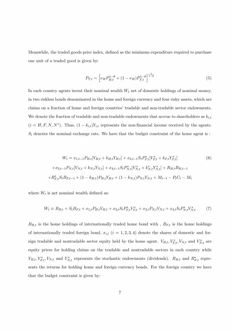
Meanwhile, the traded goods price index, de�ned as the minimum expenditure required to purchase

one unit of a traded good is given by:

PT;t =h�HP

1��H;t + (1� �H)P

1��F;t

i 11��

(5)

In each country agents invest their nominal wealth Wt net of domestic holdings of nominal money,

in two riskless bonds denominated in the home and foreign currency and four risky assets, which are

claims on a fraction of home and foreign countries�tradable and non-tradable sector endowments.

We denote the fraction of tradable and non-tradable endowments that accrue to shareholders as ki;t

(i = H;F;N;N�). Thus, (1 � ki;t)Yi;t represents the non-�nancial income received by the agents.

St denotes the nominal exchange rate. We have that the budget constraint of the home agent is :

Wt = x1;t�1PH;t[VH;t + kH;tYH;t] + x2;t�1StP�F;t[V

�F;t + kF;tY

�F;t] (6)

+x3;t�1PN;t[VN;t + kN;tYN;t] + x4;t�1StP�N;t[V

�N;t + k

�N;tY

�N;t] +RH;tBH;t�1

+R�F;tStBF;t�1 + (1� kH;t)PH;tYH;t + (1� kN;t)PN;tYN;t +Mt�1 � PtCt �Mt

where Wt is net nominal wealth de�ned as:

Wt � BH;t + StBF;t + x1;tPH;tVH;t + x2;tStP �F;tV �F;t + x3;tPN;tVN;t + x4;tStP �N;tV �N;t (7)

BH;t is the home holdings of internationally traded home bond with , BF;t is the home holdings

of internationally traded foreign bond, xi;t (i = 1; 2; 3; 4) denote the shares of domestic and for-

eign tradable and nontradable sector equity held by the home agent. VH;t; V �F;t; VN;t and V�N;t are

equity prices for holding claims on the tradable and nontradable sectors in each country while

YH;t; Y�F;t; YN;t and Y

�N;t represents the stochastic endowments (dividends). RH;t and R

�F;t repre-

sents the returns for holding home and foreign currency bonds. For the foreign country we have

that the budget constraint is given by:

7

W �t = x

�1;t�1

PH;tSt[VH;t + kH;tYH;t] + x

�2;t�1P

�F;t[V

�F;t + kF;tY

�F;t] (8)

+x�3;t�1PN;tSt[VN;t + kN;tYN;t] + x

�4;t�1P

�N;t[V

�N;t + k

�N;tY

�N;t] +

RH;tSt

B�H;t�1

+R�F;tB�F;t�1 + (1� kF;t)PF;tYF;t + (1� k�N;t)P �N;tY �N;t +M�

t�1 � P �t C�t �M�t

where

W �t �

B�H;tSt

+B�F;t + x�1;t

PH;tStVH;t + x

�2;tP

�F;tV

�F;t + x

�3;t

PN;tStVN;t + x

�4;tP

�N;tV

�N;t (9)

Gross nominal equity returns and bonds returns expressed in terms of the home currency are

as follows:

R1;t �PH;t[VH;t + kH;tYH;t]

PH;t�1VH;t�1; R2;t �

StP�F;t[V

�F;t + kF;tY

�F;t]

St�1P �F;t�1V�F;t�1

(10)

R3;t �PN;t[VN;t + kN;tYN;t]

PN;t�1VN;t�1; R4;t �

StP�N;t[V

�N;t + k

�N;tY

�N;t]

St�1P �N;t�1V�N;t�1

R5;t � R�F;tStSt�1

; R6;t � RH;t

Vi and Yi are in units of the index good i; where i = H;F;N;N�. We multiply them by the price

of the respective index good, Pi; to �nd the nominal equity return expressed in home currency2.

2The real returns will depend on the relative price of each index good with respect to the overall price level P :

8

We can express home agents�asset holdings as shares of wealth:3

x1;tPH;tVH;t � �1;tWt; x2;tStP�F;tV

�F;t � �2;tWt (12)

x3;tPN;tVN;t � �3;tWt; x4;tStP�N;tV

�N;t � �4;tWt

StBF;t � �5;tWt; BH;t � �6;tWt

6Xi=0

�i;t = 1:

Using the de�nition of gross nominal returns as in (10) and the shares of wealth invested in

assets as de�ned in (12), we can rewrite the budget constraint in terms of excess returns over the

r1;t = R1;tPt�1Pt

�PH;tPt[VH;t + YH;t]

PH;t�1Pt�1

VH;t�1; r2;t � R2;t

Pt�1Pt

=

StP�F;t

Pt[V �F;t + Y

�F;t]

St�1;fP�F;t�1Pt�1

V �F;t�1

r3;t � R3;tPt�1Pt

=

PN;tPt[VN;t + YN;t]

PN;t�1Pt

VN;t�1; r4;t = R4;t

Pt�1Pt

�StP

�N;t

Pt[V �N;t + Y

�N;t]

St�1P�N;t�1Pt

V �N;t�1

r5;t = R5;tPt�1Pt

, r6;t = R6;tPt�1Pt

3Foreign agent�s asset holdings as shares of wealth are de�ned as:

x�1;tPH;tVH;tSt

� ��1;tW �t ; x

�2;tP

�F;tV

�F;t � ��2;tW �

t (11)

x�3;tPN;tVN;tSt

� ��3;tW �t ; x

�4;tP

�N;tV

�N;t � ��4;tW �

t

B�F;t � ��5;tW �

t ;B�H;t

St� ��6;tW �

t

6Xi=0

��i;t = 1

9

return on the home bond, Rxi = Ri;t �R6;t where i = 1; ::::; 54:

Wt = [Rx1;t�1;t�1 +Rx2;t�2;t�1 +Rx3;t�3;t�1 +Rx4;t�4;t�1 +Rx5;t�5;t�1 +R6;t]Wt�1 (14)

+(1� kH;t)PH;tYH;t + (1� kN;t)PN;tYN;t � PtCt � (Mt �Mt�1)

3.2 Policy rules

We close the model by considering alternative policy rules. Although prices are fully �exible in our

model, the way we specify policy rules matters as long as we have a nominal asset. This is because

the return di¤erential between home and foreign bonds is given by the rate of (unexpected) nominal

exchange depreciation, which is a¤ected by the policy rule in a �exible price setting. Consequently,

equilibrium portfolio shares will be a¤ected, which will then feed back into the model.

We focus on two cases: in the �rst one, policy authorities stabilize their own tradable prices

(PH;t = 1;and PF �;t = 1) and in the second one they stabilize domestic consumer prices (Pt = 1;and

P �t = 1): Once we close the model the �rst order conditions that determine real money balances will

determineMt andM�t as a residual. Having a nominal bond with a CPI targeting rule is equivalent

to having a real bond (or CPI indexed bond) with any policy rule in terms of equilibrium portfolio

and model solution. Thus to facilitate discussion, we treat bonds under these two di¤erent policy

speci�cations as di¤erent assets: we will refer to the nominal bond under CPI targeting rule as the

real bond.4Similarly, the budget constraint of the foreign agent can be expressed in terms of excess returns as:

W �t =

St�1St

[Rx1;t��1;t�1 +Rx2;t�

�2;t�1 +Rx3;t�

�3;t�1 +Rx4;t�

�4;t�1 +Rx5;t�

�5;t�1 +R6;t]W

�t�1 (13)

(1� kF;t)PF;tYF;t + (1� k�N;t)P �N;tY �N;t � P �t C�t � (M�

t �M�t�1)

10

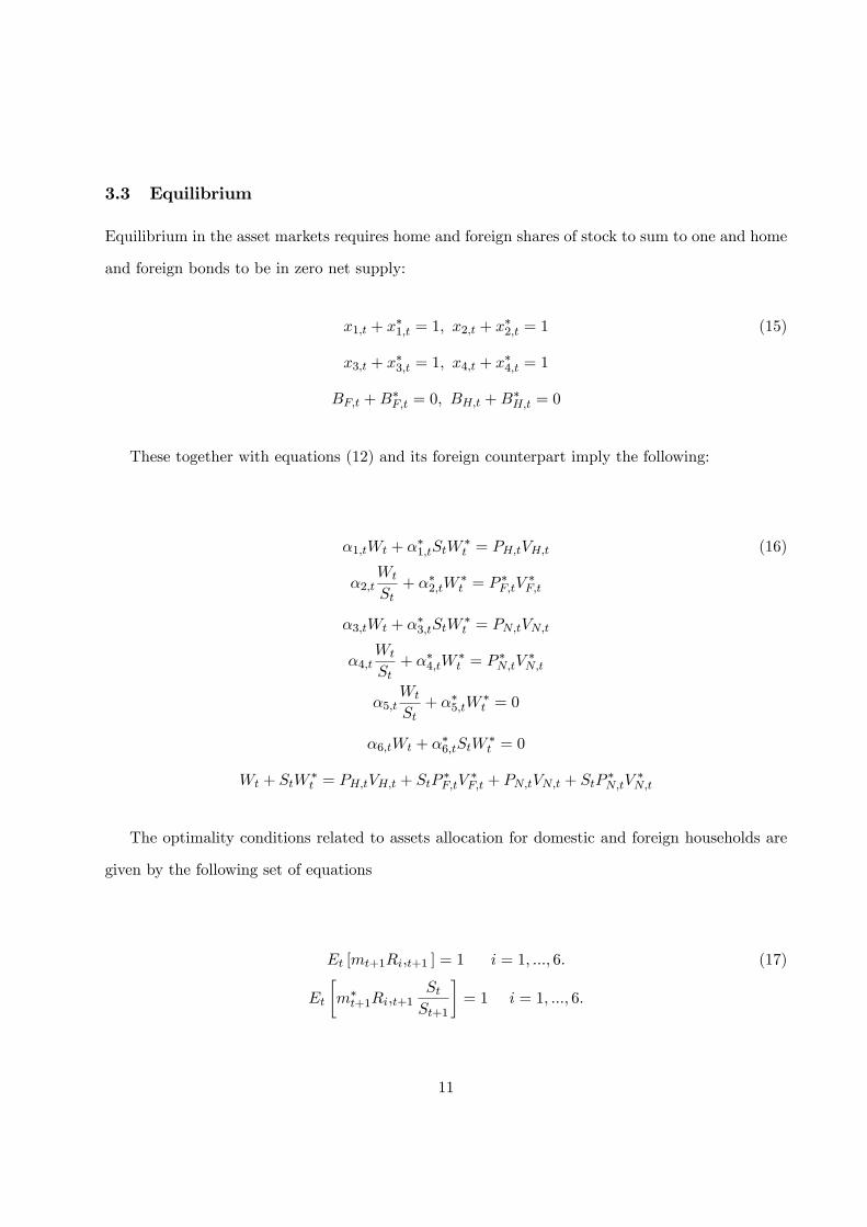
3.3 Equilibrium

Equilibrium in the asset markets requires home and foreign shares of stock to sum to one and home

and foreign bonds to be in zero net supply:

x1;t + x�1;t = 1; x2;t + x

�2;t = 1 (15)

x3;t + x�3;t = 1; x4;t + x

�4;t = 1

BF;t +B�F;t = 0; BH;t +B

�H;t = 0

These together with equations (12) and its foreign counterpart imply the following:

�1;tWt + ��1;tStW

�t = PH;tVH;t (16)

�2;tWt

St+ ��2;tW

�t = P

�F;tV

�F;t

�3;tWt + ��3;tStW

�t = PN;tVN;t

�4;tWt

St+ ��4;tW

�t = P

�N;tV

�N;t

�5;tWt

St+ ��5;tW

�t = 0

�6;tWt + ��6;tStW

�t = 0

Wt + StW�t = PH;tVH;t + StP

�F;tV

�F;t + PN;tVN;t + StP

�N;tV

�N;t

The optimality conditions related to assets allocation for domestic and foreign households are

given by the following set of equations

Et [mt+1Ri;t+1 ] = 1 i = 1; :::; 6: (17)

Et

�m�t+1Ri;t+1

StSt+1

�= 1 i = 1; :::; 6:

11

where mt+1 = �PtPt+1

�CtCt+1

��and m�

t+1 = �P �tP �t+1

�C�tC�t+1

��.

In what follows we also assume that there is complete pass-through, i.e. PH�;t = PH;t=St;and

PF;t = PF �;tSt: Equilibrium conditions in the good markets are obtained by equalizing the supply

of each good with the demand obtained from the consumer intratemporal maximization problem.

YH;t =

�PH;tPT;t

��� �PT;tPt

��� H�HCt +

P �H;tP �T;t

!�� �P �T;tP �t

��� F �FC

�t

Y �F;t =

�PF;tPT;t

��� �PT;tPt

��� H(1� �H)Ct +

P �F;tP �T;t

!�� �P �T;tP �t

��� F (1� �F )C�t

YN;t =

�PN;tPt

���(1� H)Ct; Y �N;t =

�P �N;tP �t

���(1� F )C�t

Finally asset prices are determined by combining the Euler equation with the de�nition of gross

returns. Forward iteration together with no-bubble condition gives us the following:

VH;t =

1Xs=t+1

Et

(�s�t

u0(cs)PH;sPs

u0(ct)PH;tPt

kH;sYH;s

); V �F;t =

1Xs=t+1

Et

8<:�s�tu0(cs)SsP �F;sPs

u0(ct)StPF;tPt

kF;sYF;s

9=; (18)

VN;t =

1Xs=t+1

Et

(�s�t

u0(cs)PN;sPs

u0(ct)PN;tPt

kN;sYN;s

); V �N;t =

1Xs=t+1

Et

8<:�s�tu0(cs)SsP �N;sPs

u0(ct)StP �N;tPt

kN�;sY�N;s

9=;3.4 Approximated solution

To solve the model we use the approximation techniques proposed in Devereux and Sutherland

(2006a) and Tille and van Wincoop (2007). We approximate our model around the symmetric

steady state in which steady-state in�ation rates are assumed to be zero (see the appendix). Given

our normalization home bias is the fraction invested by home agents in a country equity (both

tradables ��1 and nontradables, ��3) minus the share of country�s equity in the world equity supply (in

steady state that would be �W=( �W +SW�) = 1=2: So home equity bias would arise if ��1+��3 > 1=2:

If we want to measure equity bias in tradables only then the share of home country�s traded sector

12

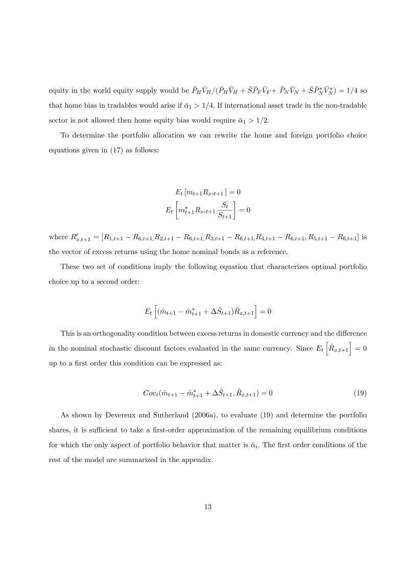
equity in the world equity supply would be �PH �VH=( �PH �VH + �S �PF �VF+ �PN �VN + �S �P �N�V �N ) = 1=4 so

that home bias in tradables would arise if ��1 > 1=4: If international asset trade in the non-tradable

sector is not allowed then home equity bias would require ��1 > 1=2:

To determine the portfolio allocation we can rewrite the home and foreign portfolio choice

equations given in (17) as follows:

Et [mt+1Rx;t+1 ] = 0

Et

�m�t+1Rx;t+1

StSt+1

�= 0

where R0x;t+1 = [R1;t+1 � R6;t+1;R2;t+1 � R6;t+1;R3;t+1 � R6;t+1;R4;t+1 � R6;t+1; R5;t+1 � R6;t+1] is

the vector of excess returns using the home nominal bonds as a reference.

These two set of conditions imply the following equation that characterizes optimal portfolio

choice up to a second order:

Et

h(mt+1 � m�

t+1 +�St+1)Rx;t+1

i= 0

This is an orthogonality condition between excess returns in domestic currency and the di¤erence

in the nominal stochastic discount factors evaluated in the same currency. Since EthRx;t+1

i= 0

up to a �rst order this condition can be expressed as:

Covt(mt+1 � m�t+1 +�St+1; Rx;t+1) = 0 (19)

As shown by Devereux and Sutherland (2006a), to evaluate (19) and determine the portfolio

shares, it is su¢ cient to take a �rst-order approximation of the remaining equilibrium conditions

for which the only aspect of portfolio behavior that matter is ��i: The �rst order conditions of the

rest of the model are summarized in the appendix.

13

4 Calibration

In this section, we outline our baseline calibration. We assume that the home and foreign economy

are of equal size and are calibrated in a symmetric fashion. In choosing the parameters of utility

function, we set � to match a 4% annual discount rate. As in Stockman and Tesar (1995) the coe¢ -

cient of constant relative risk aversion, or the inverse of the intertemporal elasticity of substitution,

�, is set to 2.

We calibrate the parameters pertaining to the consumption basket in the following way. The

share of tradable goods in �nal consumption, ; is 0.55, while the share of home goods in tradable

consumption, �; is 0.72. The calibration of this parameter is in line with other recent studies, such

as Corsetti et al. (2008).

We assume an elasticity of substitution between home and foreign traded goods, �, of 2.5 and

an elasticity of substitution between traded and non-traded goods, �; of 0.41, similar to what is

suggested by Stockman and Tesar (1995)5. Given � = 2; this implies that utility is non-separable

between traded and non-traded goods. Indeed, traded and non-traded goods are complements in

our benchmark calibration since �� < 1.

At �rst pass we proxy our process for tradable and non-tradable endowments in terms of the

corresponding Solow residuals for each sector as in other studies. 6 To estimate these shocks

Benigno and Thoenissen (2007) set US as the �home� country and Japan plus the EU15 as the

�foreign�economy and use annual sectoral output and labour input from the Groningen Growth

and Development Centre, 60-Industry Database which spans the years 1979 - 2002. They follow

Backus, Kehoe and Kydland (1992) by imposing cross-country symmetry on the estimated shock

process. Accordingly, endowments (dividends) are given by the following �rst order autoregressive

process:

5Ostry and Reinhart (1992) estimate this parameter to be higher in the range of 0.66-1.446See Benigno and Thoenissen (2007), Corsetti et al (2008), Matsumoto (2007) and Stockman and Tesar (1995).

14

266666664

log YH;t

log Y �F;t

log YN;t

log Y �N;t

377777775=

266666664

�T 0 0 0

0 �T 0 0

0 0 �N 0

0 0 0 �N

377777775

266666664

log YH;t�1

log Y �F;t�1

log YN;t�1

log Y �N;t�1

377777775+

266666664

�H;t

��F;t

�N;t

��N;t

377777775(20)

where �T = 0:84 and �N = 0:30 . For the variance-covariance matrix of endowment shocks, we

set V (�H) = V (�F ) = 3:76 and V (��N ) = V (��N ) = 0:51: We set the covariance between tradable

and non-tradable endowments to zero at �rst pass to examine the role of the relative variance in

determining the equilibrium portfolio and cross correlations.

In calibrating redistributive shocks we follow Coeurdacier, Kollman and Martin (2007). They

compute the steady-state capital share to be 40% using data for G7 countries. Thus we set the

mean capital share in tradable sector as �kH = 0:4 and assume that the mean capital share in the

non-tradable sector will be lower at �kn = 0:2: Since under incomplete markets what matters for

optimal portfolio is the relative size of shocks, we use the standard deviations of capital share and

real GDP growth calculated by Coeurdacier et al. (2007) and set the relative size of redistributive

versus endowment shocks to V (�Ki)=V (�Y i) = 1:2 for i = H;F;N;N�:The autoregressive process

considered for redistributive shocks are as follows:

266666664

log kH;t

log k�F;t

log kN;t

log k�N;t

377777775=

266666664

�KT 0 0 0

0 �KT 0 0

0 0 �KN 0

0 0 0 �KN

377777775

266666664

log kH;t�1

log k�F;t�1

log kN;t�1

log k�N;t�1

377777775+

266666664

�kH ;t

��kF ;t

�kN ;t

��kN ;t

377777775(21)

Assuming redistributive shocks to be equally persistent as tradable endowment shocks we set

�KT = �KN = �T = 0:84:

After solving the model in terms of the state variables, we use these autoregressive processes to

generate simulated time series of length T for the variables of interest and compute the moments

of interest (standard deviation, covariances). We repeat this procedure J times and then compute

15

the average of the moments. We compute the moments based on these Monte Carlo simulations

because, under certain speci�cations, i.e. incomplete markets, our model is non-stationary.

5 Results

Before going into the details of each asset market structure we consider, we give an overview of

how optimal portfolio shares and degree of international risk sharing vary across di¤erent degrees

of �nancial market integration. The most basic �nancial market structure we consider is where

there is international trade in only one non-contingent bond. Then we consider intermediate cases

where only bonds or equities are internationally traded. The most complex asset market structure

that we consider is the case in which all equities and bonds can be traded. Table 1 reports the

results for the case where uncertainty is solely driven by shocks to tradable and non-tradable sector

endowments while Table 2 considers redistributive shocks as additional sources of risk.

According to the spanning principle, markets will be potentially incomplete as long as the

number of independent shocks hitting the economy is bigger than the number of assets available for

trade. However, Table 1 shows that even with trade in only nominal bonds or trade in only tradable

sector equities, full international risk sharing can be achieved when there are only endowment

shocks. When redistributive shocks are added, full risk sharing can only be achieved with the most

complex asset market con�guration, where trade in all equities and bonds is possible.

Our results suggest that full international risk sharing can be consistent with a home or a foreign

bias depending on the model speci�cation. Full risk sharing-as re�ected by a perfect correlation

between relative consumption and real exchange rate- is consistent with both a foreign bias (the

case with 2 tradable equity and 4 endowment shocks, Table 1), and a home bias ( the case with 4

equities and 2 nominal bonds with redistributive shocks, Table 2).

Tables 1 and 2 also suggest that adding more sources of uncertainty while keeping the asset

market structure unchanged, yields a switch from foreign equity bias to home equity bias, while

decreasing the degree international risk sharing. To put it di¤erently, moving towards a world with

16

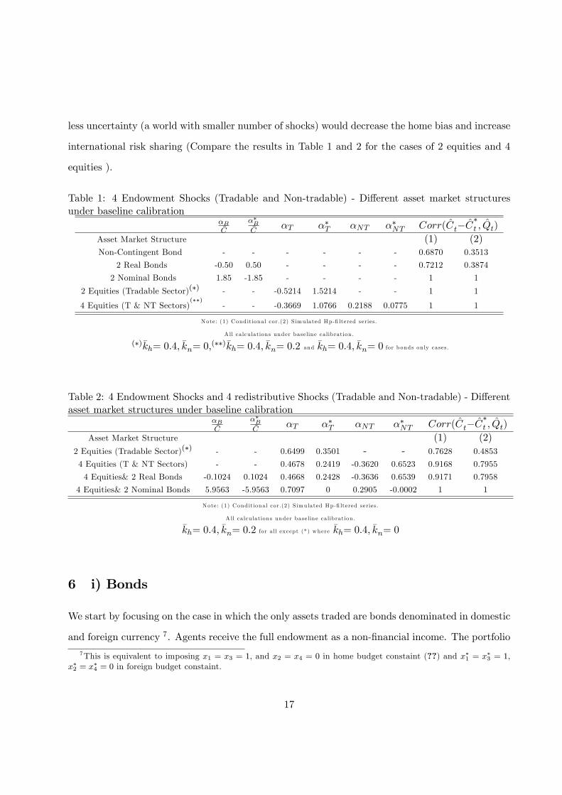
less uncertainty (a world with smaller number of shocks) would decrease the home bias and increase

international risk sharing (Compare the results in Table 1 and 2 for the cases of 2 equities and 4

equities ).

Table 1: 4 Endowment Shocks (Tradable and Non-tradable) - Di¤erent asset market structuresunder baseline calibration

�B�C

��B�C

�T ��T �NT ��NT Corr(Ct�C�t ; Qt)

Asset Market Structure (1) (2)Non-Contingent Bond - - - - - - 0.6870 0.3513

2 Real Bonds -0.50 0.50 - - - - 0.7212 0.3874

2 Nominal Bonds 1.85 -1.85 - - - - 1 1

2 Equities (Tradable Sector)(�) - - -0.5214 1.5214 - - 1 1

4 Equities (T & NT Sectors)(��)

- - -0.3669 1.0766 0.2188 0.0775 1 1

Note: (1) Conditional cor.(2) S imulated Hp-�ltered series.

A ll ca lcu lations under baseline calibration .

(�)�kh= 0:4; �kn= 0;(��)�kh= 0:4; �kn= 0:2 and �kh= 0:4; �kn= 0 for b onds on ly cases.

Table 2: 4 Endowment Shocks and 4 redistributive Shocks (Tradable and Non-tradable) - Di¤erentasset market structures under baseline calibration

�B�C

��B�C

�T ��T �NT ��NT Corr(Ct�C�t ; Qt)

Asset Market Structure (1) (2)

2 Equities (Tradable Sector)(�) - - 0.6499 0.3501 - - 0.7628 0.4853

4 Equities (T & NT Sectors) - - 0.4678 0.2419 -0.3620 0.6523 0.9168 0.7955

4 Equities& 2 Real Bonds -0.1024 0.1024 0.4668 0.2428 -0.3636 0.6539 0.9171 0.7958

4 Equities& 2 Nominal Bonds 5.9563 -5.9563 0.7097 0 0.2905 -0.0002 1 1

Note: (1) Conditional cor.(2) S imulated Hp-�ltered series.

A ll ca lcu lations under baseline calibration .

�kh= 0:4; �kn= 0:2 for a ll except (*) where �kh= 0:4; �kn= 0

6 i) Bonds

We start by focusing on the case in which the only assets traded are bonds denominated in domestic

and foreign currency 7. Agents receive the full endowment as a non-�nancial income. The portfolio

7This is equivalent to imposing x1 = x3 = 1; and x2 = x4 = 0 in home budget constaint (??) and x�1 = x�3 = 1;x�2 = x

�4 = 0 in foreign budget constaint.

17

orthogonality condition given in terms of the relative pricing kernel in (19) can be written in terms

of real exchange rate adjusted relative consumption and excess return on foreign bonds:

Covt(Ct+1 � C�t+1 �Qt+1�; Rx;t+1) = 0 (22)

with Rx;t = RF;t � RH;t: As discussed in Section 3, policy rules matter for portfolio choice since

we are in the presence of nominal bonds. Thus in our analysis of bond portfolios we distinguish

among di¤erent policy rules, focusing on special parametric cases for the analytical solution.

a) Domestic tradable price targeting, PH;t = 0 and P �F;t = 0

When there is no consumption home bias (� = 1� � = 0:5) the optimal bond portfolio position

is:

~�B = �~�B� = (� � 1)2(1� ��T )

(23)

We note here that domestic households will be long in the domestic bond as long as � > 1:

Moreover the bond position (in this special case) is not a¤ected by shocks to the non-traded sector

or volatility of both shocks. To explain this portfolio position it is useful to consider what would

happen to the components of the portfolio orthogonality condition given in (22) in the case in which

each country had a zero portfolio share (~�B = �~�B� = 0): In particular we are interested in the

zero portfolio solution of the relative consumption and the excess returns:

Ct�C�t �Qt�=1

��

�� � 1�

1� �(1� ��T )

+� � 1�

(��� 1)(1� ��T )

�(�H;t � �F;t)+

(1� )(��� 1)(1� ��N )

(�N;t���N;t)

(24)

Rx;t = RF;t � RH;t = St � Et�1St =1

�(�H;t � �F;t) (25)

Without any portfolio diversi�cation, (24) shows that in response to a positive home country

tradable shock, home relative consumption rises as long as � > 1 and �� > 1 (tradable and

non-tradable goods are gross substitutes). If �� < 1 (i.e. the tradable and non-tradable are gross

complements) agents would prefer to increase consumption of both tradable and non-tradable goods:

18

the fact that the supply of non-tradables has not changed prevent them for doing so, creating a

possible negative e¤ect on overall consumption. Still, for plausible parameters, relative consumption

increases following a positive tradable endowment shock even when traded and non-traded goods

are complements in consumption. A similar reasoning occurs when there is a shock to non-tradable

endowment: in this case the substitutability (�� > 1 or �� < 1) matters for determining the sign

of the relative consumption response.

To hedge against the consumption risk (captured by movements in (24)), agents would like to

hold domestic currency bonds when their return falls following an increase in relative consumption.

Indeed (25) shows that following a positive shock to home tradable endowment, excess return on

home bonds falls, i.e. Rx;t rises, as the nominal exchange rate depreciates. Thus home bonds

provide a good hedge against traded sector shocks for � > 1:We note here that excess return is not

a¤ected at all by the substitutability or complementarity of traded and non-traded goods or the

presence of non-traded goods shocks: thus, agents cannot hedge against non-traded sector shocks

when there is no consumption home bias and the only assets available are currency bonds.

When utility is separable (�� = 1) the optimal bond portfolio position is:

~�B = �~�B� = (1� �)(�� 1 + 2�(� � �))

(1� ��T )(26)

Since in this case � = 1� , it is possible to rewrite the above expression as follows (� = 1 gives

the log-investor under separable utility):

~�B = �~�B� = (1� �)(1� ��T )

���� 1

�+ 2�(� � 1

�)

�(27)

As before the bond position is not a¤ected by shocks to the non-traded sector or volatility of

the shocks. As long as there is consumption home bias (� > 1=2) home currency holdings will be

positive. When each country has a zero portfolio share (~�B = �~�B� = 0): the real exchange rate

19

adjusted consumption di¤erential and the excess returns are given by:

Ct � C�t �Qt�=

1� �1� ��T

(�� 1 + 2�(� � �))(1 + 2�(� � 1)) (�H;t � �F;t) (28)

Rx;t = RF;t � RH;t = St � Et�1St (29)

= f�(1� 4�(1� �)) + 4��(1� �) + �(2� � 1)(�� 1 + 2�(� � �))(�(2� � 1)2 + 4�(1� �)�)(1 + 2�(� � 1))(1� ��T )

+��T

(�(2� � 1)2 + 4�(1� �)�)(1� ��T )g (�H;t � �F;t)

With separable utility relative consumption and excess returns are una¤ected by shocks to

non-traded sector endowment as shown by (28) and (29). When there is a positive endowment

shock in the traded goods sector, home consumption of home traded goods will increase more than

foreign consumption of home traded goods because of the home bias in consumption. Non-traded

goods will become more expensive compared to traded goods in both countries. If � > �; i.e.

the elasticity of substitution between home and foreign traded goods is bigger than the elasticity

of substitution between traded and non-traded goods; home will decrease its consumption of the

foreign traded good more than it decreases its consumption of home non-traded good. The extent

of this substitution away from foreign traded goods increases with the degree of consumption home

bias �:Thus, relative consumption increases more in the face of a traded sector shock when � > 12

and � > �: The low elasticity of substitution between traded and non-traded goods, i.e. � < 1;limits

the increase in relative consumption as consumers cannot easily substitute away from non-traded

goods which are now relatively more expensive in both countries.

Excess returns become a complicated expression when � 6= 12as shown in (29). Again the key

parameters that determine excess returns on home bonds, which is negatively related to unexpected

home currency depreciation, are the extent of consumption home bias captured by (2��1) and the

relative substitutability among home and foreign traded goods and among traded and non-traded

20

goods as given by (� � �):

For plausible parameter values, excess returns on home bonds are negative following traded

sector endowment shocks, while relative consumption is positive, which makes home bonds a good

hedge against real exchange rate �uctuations.

In general, for our calibration, in this case (PH;t = 0 and P �F;t = 0) domestic agents are long

in home currency bonds (Table 3). Once agents hold the optimal amount of currency bonds,

consumption and real exchange rate becomes perfectly correlated. Indeed, following a positive

supply-side shock to the home economy�s traded goods sector, home agents become wealthier and

demand more goods of all types. Despite this, through their portfolio allocation they share risk

with foreigners and transfer resources to them so that foreign consumption increases more than in

the zero-portfolio case [SEE FIGURE 1].

For the special case in which there is no home bias and utility is separable it is possible to derive

an analytical expression for the conditional correlation between consumption di¤erential and the

real exchange rate8:

Corrt�1(Ct � C�t ; Qt) =(1� )�

2N

�2T� �r�

(1� )2 �2N

�2T+ 2�

���2N�2T+�

� (30)

where � = (1��)2(2~�B� (��1))2 2�2(1���T )2

: From (30) we can see that once we substitute the optimal portfolio

allocation we obtain that the conditional correlation is always equal to 1 so that in this case there

is perfect international risk sharing.

b) Consumer price targeting, Pt = 0 and P �t = 0 (Real Bond)

When utility is separable (�� = 1) and there is no consumption home bias (� = 1 � � = 0:5)8The conditional correlation helps us in understanding the determinants of international risk-sharing. In the

quantitative analysis we report both the conditional cross correlation and the HP-�ltered cross correlation which isthe one comparable with the empirical evidence presented earlier.

21

the optimal bond portfolio position is:

~�B = �~�B� = (� � 1)2(1� ��T )

0@� (1� �)(1� )(� � 1)(1� )2�2�(1� ��T )

�2N�2T

1A (31)

The optimal portfolio position can be decomposed in two terms: the �rst term is the one that

correspond to the portfolio under tradable price targeting while the second term is speci�c to

consumer price targeting. Because of the second component, domestic households will be short in

the domestic bond so that ~�B < 09: Moreover, the optimal bond portfolio depends critically among

other things on the relative variance between traded and non-traded sector shocks. When there

are only non-tradable shocks �2N�2T

! 1, ~�B �! 0. As before we consider what would happen in

the case in which each country had a zero portfolio share (~�B = �~�B� = 0): In particular we are

interested in the behavior of the two components of the portfolio orthogonality condition-relative

consumption and the excess returns:

Ct � C�t �Qt�=� � 1�

1� �(1� ��T )

(�H;t � �F;t) (33)

Rx;t = RF;t � RH;t = St � Et�1St = Qt � Et�1Qt (34)

=1

�

�(1� �)(1� )(� � 1)

��(1� ��T )

�(�H;t � �F;t) +

1� �

��N;t � ��N;t

�From (34) we can see the link between optimal bond position and the excess return on for-

eign bonds. Following a positive tradable endowment shock, under consumer price targeting, the

9Under non-separability the expression that determines the optimal portfolio position is more complicated andthe sign of the bond position depends on the degree of substitutability between tradable and non-tradable:

~�B = �~�B� = ��� � 1�

�2�1� �

2(1� ��T )2

���2N�2T

��1 (1 + (��� 1))2 (1� ��N )

�(1� )� (32)

+ (��� 1)2�(1� ��N )

where � = ��(1� ��N )� (1� �)(1� )(��� 1):

22

exchange rate appreciate as long as � > 1: Home consumption on the other hand will increase com-

pared to foreign consumption following the same positive tradable endowment shock. This implies

that domestic bonds will be a poor hedge against consumption risk if tradable shocks are the main

source of uncertainty. On the other hand, following a positive non-tradable endowment shock, ex-

cess return on home bonds will be higher while relative consumption will remain unchanged. This

would also discourage holdings of home bonds 10

In general, for our calibration, in this case (Pt = 0 and P �t = 0) domestic agents are short

in home currency bonds (Table 3). Once agents hold the optimal amount of currency bonds,

consumption and real exchange rate becomes imperfectly correlated. Indeed, following a positive

supply-side shock to the home economy�s traded goods sector, home agents become wealthier and

demand more goods of all types. In this case there is no enough risk-sharing either through portfolio

allocation or the terms of trade and because of this foreign consumption does not increase by as

much as home consumption. Also the real exchange rate appreciates since the Balassa-Samuelson

e¤ect dominates the terms of trade e¤ect [SEE FIGURE 2].

For the special case in which there is no home bias and utility is separable it is possible to derive

an analytical expression for the conditional correlation between consumption di¤erential and the

real exchange rate:

10Under non-separability we have more complicated expression for the consumption di¤erential and the excessreturn:

Ct � C�t �Qt�=� � 1�

1� �(1� ��T )

1 + (��� 1)��

(�H;t � �F;t) (35)

+1� �

(1� ��N )(1� )(��� 1)

��

��N;t � ��N;t

�

Rx;t = RF;t � RH;t = St � Et�1St

= �� � 1�

1� �(1� ��T )

1� �

(�H;t � �F;t) (36)

+1� �

�

(1 + (��� 1)) (1� ��N )��N;t � ��N;t

�

23

Corrt�1(Ct � C�t ; Qt) =�(1� )�1�2

�2N�2T+ � 2�r�

(1� )2�21�2N�2T+ (� 2)2�

���22

�2N�2T+�

� (37)

where

�1 =2~�B(1� �)� �(1� ��N )

2~�B(1� �)(1� )� �(1� ��N )

�2 =(1� ��N )

2~�B(1� �)(1� )� �(1� ��N )

� =

�� � 1�

1� �2~�B(1� �)(1� )� �(1� ��T )

�2

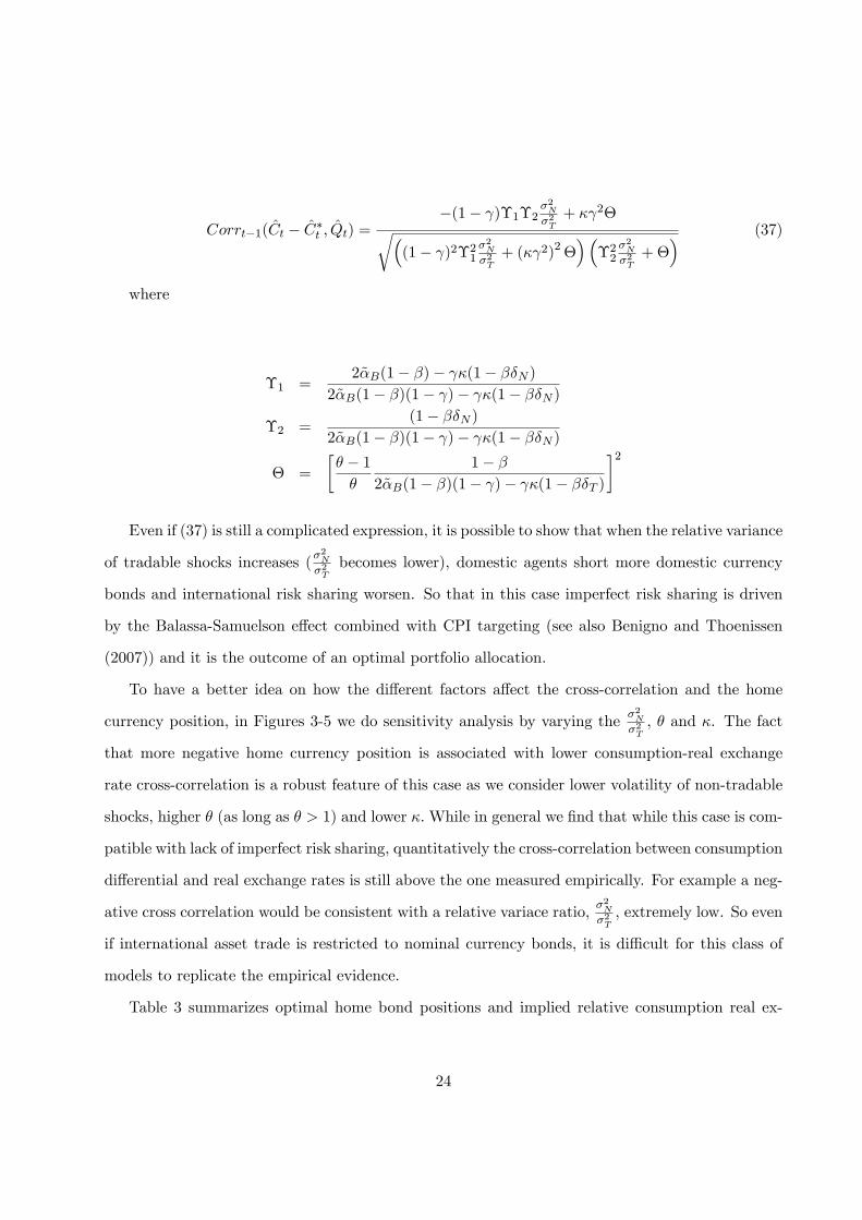
Even if (37) is still a complicated expression, it is possible to show that when the relative variance

of tradable shocks increases (�2N

�2Tbecomes lower), domestic agents short more domestic currency

bonds and international risk sharing worsen. So that in this case imperfect risk sharing is driven

by the Balassa-Samuelson e¤ect combined with CPI targeting (see also Benigno and Thoenissen

(2007)) and it is the outcome of an optimal portfolio allocation.

To have a better idea on how the di¤erent factors a¤ect the cross-correlation and the home

currency position, in Figures 3-5 we do sensitivity analysis by varying the �2N�2T; � and �. The fact

that more negative home currency position is associated with lower consumption-real exchange

rate cross-correlation is a robust feature of this case as we consider lower volatility of non-tradable

shocks, higher � (as long as � > 1) and lower �:While in general we �nd that while this case is com-

patible with lack of imperfect risk sharing, quantitatively the cross-correlation between consumption

di¤erential and real exchange rates is still above the one measured empirically. For example a neg-

ative cross correlation would be consistent with a relative variace ratio, �2N

�2T, extremely low. So even

if international asset trade is restricted to nominal currency bonds, it is di¢ cult for this class of

models to replicate the empirical evidence.

Table 3 summarizes optimal home bond positions and implied relative consumption real ex-

24

change rate correlations under the two policy rules we consider for our benchmark calibration and

for the special cases of symmetric prefences and separable utility.

Table 3: 2 Nominal Bonds, 4 Endowment Shocks - Baseline model and sensitivity analysis

Home bondsCovt(Rx;t;Qt)

V ar(Rx;t)Corr(Ct�C�t ; Qt)

�= �C (1) (2) (1) (2)

PH;t= 0 and P�F;t= 0

Baseline calibration 1.85 0.2088 0.2095 1 1

� = 0:5 2.06 0.0000 -0.0021 1 1

� = 0:5 1.83 0.2420 0.2420 1 1

Pt= 0 and P�F;t= 0

Baseline calibration -0.50 1 0.9830 0.7212 0.3874

� = 0:5 -0.83 1 0.9853 0.8142 0.5265

� = 0:5 -0.23 1 0.9832 0.7298 0.4511

Note: (1) Conditional (2) Simulated Hp-�ltered series. Rx;t=RF;t�RH;t,i.e. excess return on foreign bonds.

6.1 ii) Equities

6.1.1 Tradable sector equities

We now focus on another incomplete asset market structure in which we only allow for international

trade in tradable sector equities. This case is obtained by letting BH = BF = 0, x3 = 1 and x4 = 0

in home budget constraint given by (6) and B�H = B�F = 0, x�3 = 0 and x

�4 = 1 in foreign budget

constraint given by (8). Recall that in this case home equities bias in tradable would require

��T > 1=2 since world equities supply consists only of tradable equities.

We distinguish di¤erent cases depending on the number of shocks and the fraction of the en-

dowment which is distributed to household (i.e �labor income�) (See Table 4). In order to generate

home bias for our baseline calibration we need to have redistributive shocks as in the analysis of

Coeurdacier, Kollman and Martin (2007). Without redistributive shocks, agents go long on foreign

equity the bigger is the share of labor income. Intuitively when the share of labor income increases,

foreign equities becomes a better hedge against domestic shock so that agents tend to reduce their

25

home equity position. In the presence of redistributive shocks because of uncertainty related to

the fraction of labor income, households will tend to have more domestic equities. In general the

presence of redistributive shocks does not a¤ect the consumption di¤erential at the zero portfolio

solution (i.e. Ct� C�t � Qt� depends only on tradable and non-tradable endowment shocks) while it

does a¤ect the excess return since, for example, a positive redistributive shock that increase labor

income reduces the return on home equities. This is why foreign equities are not a good hedge

against redistributive shocks and agents increase holdings of domestic tradable equities. This e¤ect

is bigger the bigger the size of the redistributive shock relative to tradable endowment shock [SEE

FIGURE 7].

In the case with endowment shocks only, international risk-sharing is perfect despite the presence

of non-tradable shocks: by choosing optimally their portfolio of tradable equities agents perfectly

insure themselves against �uctuations in relative consumption.On the other hand, the presence of

redistributive shocks tend to lower the cross correlation between consumption and real exchange

rate. Relative consumption and real exchange rate cam move in opposite directions in the face of

a tradable endowment shock [SEE FIGURE 6]. As in the only bonds case, decreasing the relative

volatility of non-tradable shocks, (�2N

�2T) reduces the degree of risk-sharing but it doesn�t have any

e¤ect on the share of tradable equities; the higher is the elasticity of intratemporal substitution

(for � > 1) the lower is the consumption real exchange rate cross-correlation but the lower is the

degree of home bias [SEE FIGURES 8 AND 9]. In the presence of redistributive shocks, since the

equities also hedge against �uctuations in non-�nancial income in addition to �uctuations in real

exchange rate, the covariance-variance ratio of excess returns and real exchange rate decreases and

becomes more in line with data reported in van Wincoop and Warnock (2007).

In terms of the empirical evidence discussed at the beginning, this case suggests that a model

with international asset trade in tradable sector equities would be consistent with imperfect risk-

sharing and home bias in equities as long as there are redistributive shocks. From a quantitative

point of view, though, the cross-correlation between consumption di¤erential and the real exchange

rate is still above the one observed in the data. The presence of non-tradable shocks contributes

26

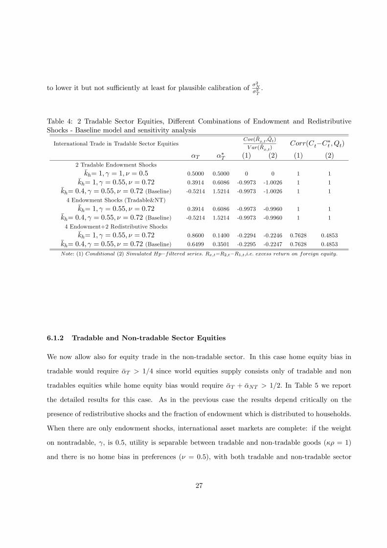
to lower it but not su¢ ciently at least for plausible calibration of �2N

�2T.

Table 4: 2 Tradable Sector Equities, Di¤erent Combinations of Endowment and RedistributiveShocks - Baseline model and sensitivity analysis

International Trade in Tradable Sector EquitiesCov(Rx;t;Qt)

V ar(Rx;t)Corr(Ct�C�t ; Qt)

�T ��T (1) (2) (1) (2)

2 Tradable Endowment Shocks�kh= 1; = 1; � = 0:5 0.5000 0.5000 0 0 1 1

�kh= 1; = 0:55; � = 0:72 0.3914 0.6086 -0.9973 -1.0026 1 1�kh= 0:4; = 0:55; � = 0:72 (Baseline) -0.5214 1.5214 -0.9973 -1.0026 1 1

4 Endowment Shocks (Tradable&NT)�kh= 1; = 0:55; � = 0:72 0.3914 0.6086 -0.9973 -0.9960 1 1

�kh= 0:4; = 0:55; � = 0:72 (Baseline) -0.5214 1.5214 -0.9973 -0.9960 1 1

4 Endowment+2 Redistributive Shocks�kh= 1; = 0:55; � = 0:72 0.8600 0.1400 -0.2294 -0.2246 0.7628 0.4853

�kh= 0:4; = 0:55; � = 0:72 (Baseline) 0.6499 0.3501 -0.2295 -0.2247 0.7628 0.4853

Note: (1) Conditional (2) Simulated Hp�filtered series: Rx;t=R2;t�R1;t;i:e: excess return on foreign equity:

6.1.2 Tradable and Non-tradable Sector Equities

We now allow also for equity trade in the non-tradable sector. In this case home equity bias in

tradable would require ��T > 1=4 since world equities supply consists only of tradable and non

tradables equities while home equity bias would require ��T + ��NT > 1=2: In Table 5 we report

the detailed results for this case. As in the previous case the results depend critically on the

presence of redistributive shocks and the fraction of endowment which is distributed to households.

When there are only endowment shocks, international asset markets are complete: if the weight

on nontradable, , is 0:5, utility is separable between tradable and non-tradable goods (�� = 1)

and there is no home bias in preferences (� = 0:5); with both tradable and non-tradable sector

27

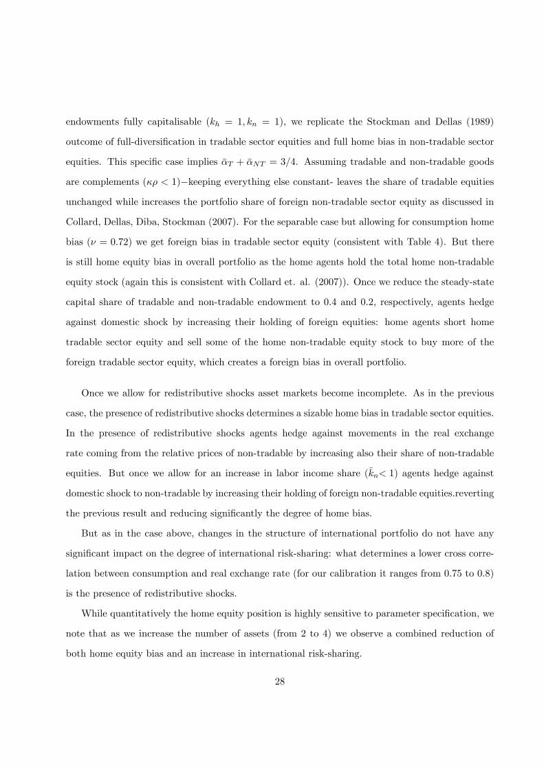
endowments fully capitalisable (kh = 1; kn = 1), we replicate the Stockman and Dellas (1989)

outcome of full-diversi�cation in tradable sector equities and full home bias in non-tradable sector

equities. This speci�c case implies ��T + ��NT = 3=4. Assuming tradable and non-tradable goods

are complements (�� < 1)�keeping everything else constant- leaves the share of tradable equities

unchanged while increases the portfolio share of foreign non-tradable sector equity as discussed in

Collard, Dellas, Diba, Stockman (2007). For the separable case but allowing for consumption home

bias (� = 0:72) we get foreign bias in tradable sector equity (consistent with Table 4). But there

is still home equity bias in overall portfolio as the home agents hold the total home non-tradable

equity stock (again this is consistent with Collard et. al. (2007)). Once we reduce the steady-state

capital share of tradable and non-tradable endowment to 0.4 and 0.2, respectively, agents hedge

against domestic shock by increasing their holding of foreign equities: home agents short home

tradable sector equity and sell some of the home non-tradable equity stock to buy more of the

foreign tradable sector equity, which creates a foreign bias in overall portfolio.

Once we allow for redistributive shocks asset markets become incomplete. As in the previous

case, the presence of redistributive shocks determines a sizable home bias in tradable sector equities.

In the presence of redistributive shocks agents hedge against movements in the real exchange

rate coming from the relative prices of non-tradable by increasing also their share of non-tradable

equities. But once we allow for an increase in labor income share (�kn< 1) agents hedge against

domestic shock to non-tradable by increasing their holding of foreign non-tradable equities.reverting

the previous result and reducing signi�cantly the degree of home bias.

But as in the case above, changes in the structure of international portfolio do not have any

signi�cant impact on the degree of international risk-sharing: what determines a lower cross corre-

lation between consumption and real exchange rate (for our calibration it ranges from 0.75 to 0.8)

is the presence of redistributive shocks.

While quantitatively the home equity position is highly sensitive to parameter speci�cation, we

note that as we increase the number of assets (from 2 to 4) we observe a combined reduction of

both home equity bias and an increase in international risk-sharing.

28

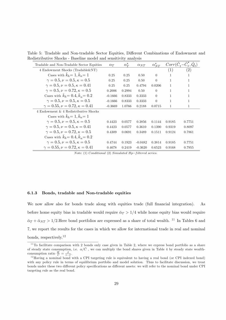
Table 5: Tradable and Non-tradable Sector Equities, Di¤erent Combinations of Endowment andRedistributive Shocks - Baseline model and sensitivity analysis

Tradable and Non-Tradable Sector Equities �T ��T �NT ��NT Corr(Ct�C�t ; Qt)

4 Endowment Shocks (Tradable&NT) (1) (2)Cases with �kh= 1; �kn= 1 0.25 0.25 0.50 0 1 1

= 0:5; � = 0:5; � = 0:5 0.25 0.25 0.50 0 1 1

= 0:5; � = 0:5; � = 0:41 0.25 0.25 0.4794 0.0206 1 1

= 0:5; � = 0:72; � = 0:5 0.2006 0.2994 0.50 0 1 1

Cases with �kh= 0:4; �kn= 0:2 -0.1666 0.8333 0.3333 0 1 1

= 0:5; � = 0:5; � = 0:5 -0.1666 0.8333 0.3333 0 1 1

= 0:55; � = 0:72; � = 0:41 -0.3669 1.0766 0.2188 0.0715 1 1

4 Endowment & 4 Redistributive Shocks

Cases with �kh= 1; �kn= 1 = 0:5; � = 0:5; � = 0:5 0.4423 0.0577 0.3856 0.1144 0.9185 0.7751

= 0:5; � = 0:5; � = 0:41 0.4423 0.0577 0.3610 0.1390 0.9319 0.8097

= 0:5; � = 0:72; � = 0:5 0.4309 0.0691 0.3489 0.1511 0.9124 0.7861

Cases with �kh= 0:4; �kn= 0:2 = 0:5; � = 0:5; � = 0:5 0.4744 0.1923 -0.0482 0.3814 0.9185 0.7751

= 0:55; � = 0:72; � = 0:41 0.4678 0.2419 -0.3620 0.6523 0.9168 0.7955

Note: (1) Conditional (2) Simulated Hp�filtered series:

6.1.3 Bonds, tradable and Non-tradable equities

We now allow also for bonds trade along with equities trade (full �nancial integration). As

before home equity bias in tradable would require ��T > 1=4 while home equity bias would require

��T + ��NT > 1=2:Here bond portfolios are expressed as a share of total wealth. 11 In Tables 6 and

7, we report the results for the cases in which we allow for international trade in real and nominal

bonds, respectively.12

11To facilitate comparison with 2 bonds only case given in Table 2, where we express bond portfolio as a shareof steady state consumption, i.e. �= �C , we can multiply the bond shares given in Table 4 by steady state wealth-consumption ratio

�W�C= �

1�� :12Having a nominal bond with a CPI targeting rule is equivalent to having a real bond (or CPI indexed bond)

with any policy rule in terms of equilibrium portfolio and model solution. Thus to facilitate discussion, we treatbonds under these two di¤erent policy speci�cations as di¤erent assets: we will refer to the nominal bond under CPItargeting rule as the real bond.

29

Compared with the only equities case, the presence of real bonds doesn�t add much: the equity

position is basically the same as in the previous case and the bond position is negative as expected.

As before we note the instability of the non-tradable equity position once we reduce the steady state

capital share of tradable and non-tradable endowment. Also there are no substantial di¤erences in

terms of cross-correlation between consumption and real exchange rate.

With nominal bonds on the other hand there is no portfolio diversi�cation: agents optimally

hold home equities both in tradable and non-tradable endowment. As in the bonds only case,

agents are long in domestic currency bonds and there is perfect international risk-sharing.

These results are consistent with recent theoretical framework that have addressed the home eq-

uity bias in various setting with market completeness or incompleteness like Coeurdacier, Kollmann

and Martin (2007, 2008), Coeurdacier and Gourinchas (2008) and Collard et al. (2007).

Despite higher �nancial integration, home equity bias is still a robust feature of the model

contradicting the empirical evidence that suggests a decline in home bias in the last decade.

Table 6: Real Bonds, Tradable and Non-Tradable Sector Equities with Endowment and Redistrib-utive Shocks - Baseline model and sensitivity analysis

Real Bonds, T and NT Equities �T ��T �NT ��NT �B ��B Corr(Ct�C�t ; Qt)

(1) (2)

Cases with �kh= 1; �kn= 1 0.4423 0.0577 0.3877 0.1123 -0.0143 0.0143 0.9228 0.7844

= 0:5; � = 0:5; � = 0:5 0.4423 0.0577 0.3877 0.1123 -0.0143 0.0143 0.9228 0.7844

= 0:5; � = 0:5; � = 0:41 0.4423 0.0577 0.3642 0.1358 -0.0137 0.0137 0.9347 0.8164

= 0:5; � = 0:72; � = 0:5 0.4306 0.0694 0.3485 0.1515 -0.0014 0.0014 0.9128 0.7866

Cases with �kh= 0:4; �kn= 0:2 = 0:5; � = 0:5; � = 0:5 0.4743 0.1923 -0.0409 0.3742 -0.0478 0.0478 0.9228 0.7844

= 0:55; � = 0:72; � = 0:41 0.4668 0.2428 -0.3636 0.6539 -0.0041 0.0041 0.9171 0.7958

Note: (1) Conditional (2) Simulated Hp�filtered series:

30

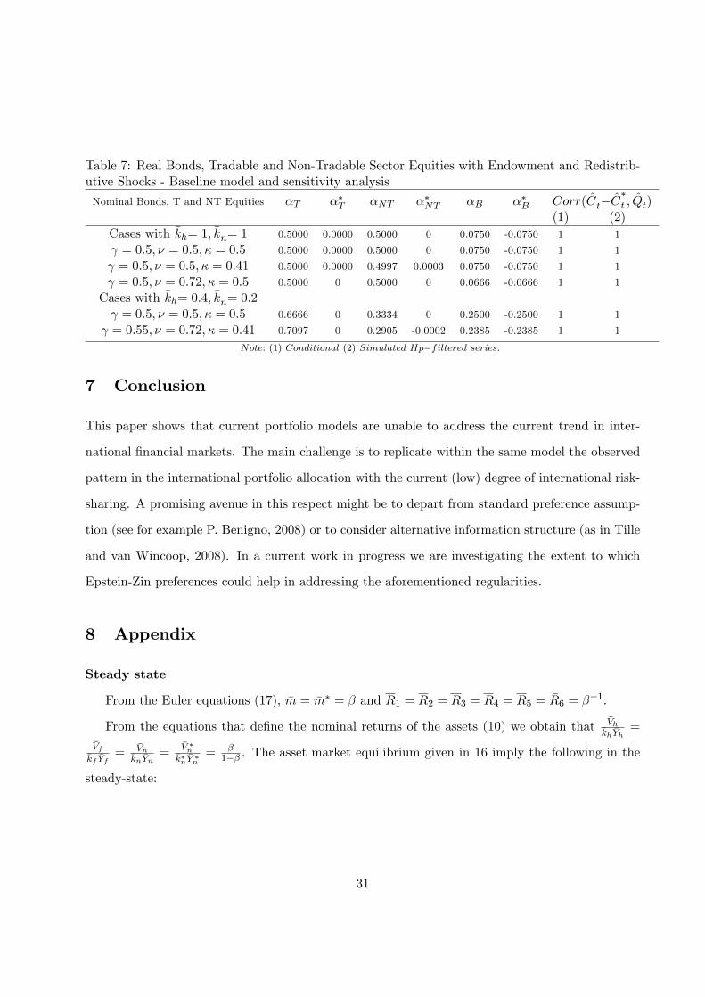
Table 7: Real Bonds, Tradable and Non-Tradable Sector Equities with Endowment and Redistrib-utive Shocks - Baseline model and sensitivity analysis

Nominal Bonds, T and NT Equities �T ��T �NT ��NT �B ��B Corr(Ct�C�t ; Qt)

(1) (2)

Cases with �kh= 1; �kn= 1 0.5000 0.0000 0.5000 0 0.0750 -0.0750 1 1

= 0:5; � = 0:5; � = 0:5 0.5000 0.0000 0.5000 0 0.0750 -0.0750 1 1

= 0:5; � = 0:5; � = 0:41 0.5000 0.0000 0.4997 0.0003 0.0750 -0.0750 1 1

= 0:5; � = 0:72; � = 0:5 0.5000 0 0.5000 0 0.0666 -0.0666 1 1

Cases with �kh= 0:4; �kn= 0:2 = 0:5; � = 0:5; � = 0:5 0.6666 0 0.3334 0 0.2500 -0.2500 1 1

= 0:55; � = 0:72; � = 0:41 0.7097 0 0.2905 -0.0002 0.2385 -0.2385 1 1

Note: (1) Conditional (2) Simulated Hp�filtered series:

7 Conclusion

This paper shows that current portfolio models are unable to address the current trend in inter-

national �nancial markets. The main challenge is to replicate within the same model the observed

pattern in the international portfolio allocation with the current (low) degree of international risk-

sharing. A promising avenue in this respect might be to depart from standard preference assump-

tion (see for example P. Benigno, 2008) or to consider alternative information structure (as in Tille

and van Wincoop, 2008). In a current work in progress we are investigating the extent to which

Epstein-Zin preferences could help in addressing the aforementioned regularities.

8 Appendix

Steady state

From the Euler equations (17), �m = �m� = � and R1 = R2 = R3 = R4 = R5 = �R6 = ��1.

From the equations that de�ne the nominal returns of the assets (10) we obtain that�Vh�kh �Yh

=

�Vf�kf �Yf

=�Vn�kn �Yn

=�V �n�k�n �Y

�n= �

1�� . The asset market equilibrium given in 16 imply the following in the

steady-state:

31

��1 �W + ���1 �S �W� = �Ph �Vh

��2�W�S+ ���2 �W

� = �P �f �V�f

��3 �W + ���3 �S �W� = �Pn �Vn

��4�W�S+ ���4 �W

� = �P �n �V�n

��5�W�S+ ���5 �W

� = 0

��6 �W + ���6 �S �W� = 0

�W + �S �W � = �Ph �Vh + �S �P �f �V�f +

�Pn �Vn + �S �Pn �V�n

As the initial wealth distribution is not determined we choose steady state net wealth as in

P. Benigno (2007) and assume �W = SW�. We normalize �ki and �Yi for i = h; f�; n; n� such that

�Ph �Vh = �S �Pf �Vf = �Pn �Vn = �S �P �n �V�h = 0:5 �W: With this normalization, steady-state asset shares

satisfy:

��1 + ���1 = 0:5

��2 + ���2 = 0:5

��3 + ���3 = 0:5

��4 + ���4 = 0:5

��5 + ���5 = 0

��6 + ���6 = 0

This normalization also implies that ��i = 0:5�xi for i = 1; :::; 4:So in our framework home bias

is the fraction invested by home agents in a country equity (both tradables ��1 and nontradables,

��3) minus the share of country�s equity in the world equity supply (in steady state that would be

�W=( �W + SW�) = 1=2: So home bias would arise if ��1 + ��3 > 1=2:

32

If we want to measure equity bias in tradables only then the share of home country�s traded

sector equity in the world equity supply would be �Ph �Vh=( �Ph �Vh + �S �Pf �Vf+ �Pn �Vn + �S �P �n �V�h ) = 1=4

so that home bias in tradables would arise if ��1 > 1=4: If international asset trade in the non-

tradable sector is not allowed then ��1 > 1=2:All relative prices are equal to 1 in the symmetric

steady-state and �S = 1: Using the goods market equilibrium conditions given in (??), we can pin

down steady-state consumption relative to tradable and nontradable sector output as follows:13

�C�YH

=�C�

�YH=

1

H�H + F �F�C�YF=�C�

�YF=

1

H(1� �H) + F (1� �F )�C�YN

=�C�

�YN=

1

1� H�C�Y �N

=�C�

�Y �N=

1

1� F

with

�CH = H�H �C; �CF = H(1� �H) �C�

�C�H = F �F �C; �C�F = F (1� �F ) �C�

First Order Approximation to the Rest of the Model:

First Order Approximation to the Rest of the Model:

For any variable y ,except Rx, we de�ne log-deviation from the steady-state, by as by = log(yty ).The log-deviation of excess return bRxi;t can be characterized as bRxi;t = Rxi;t�R

R:

Combining home and foreign Euler equations:

13Using the budget constraints, (14, 13) and normalizing resdistributive parameters so that �kh = �kf , �kn = �k�n, wecan show that steady-state consumption in home and foreign countries are equalized, i.e. �C = �C�.

33

Et

h bmt+1 � bm�t+1 + bSt+1 � bSti = 0 (38)

Home stochastic discount factor:

bmt = bPt�1 � bPt + � bCt�1 � � bCt (39)

Foreign stochastic discount factor:

bm�t =

bP �t�1 � bP �t + � bC�t�1 � � bC�t (40)

Home budget constraint:

cWt =1

�cWt�1 +

1

�bR6;t + bRx1;tf�1 + bRx2;tf�2 + bRx3;tf�3 + bRx4;tf�4 + bRx5;tf�5

+(1� �kH)�PH �YH�W

(PH;t + YH;t) + (1� �kN )�PN �YN�W

(PN;t + YN;t)� �kH�PH �YH�W

kH;t � �kN�PN �YN�W

kN;t(41)

�PCW( bPt + bCt)

where

e�i =�i�for i = 1; :::; 6:

�P �C�W

=

�1� ��

�1

1� (1� �kH)( H�H + F �F )� (1� �kN )(1� H)�PH �YH�W

=�PH �YH�P �C

�P �C�W=

�1� ��

� H�H + F vF

1� (1� �kH)( H�H + F �F )� (1� �kN )(1� H)�PN �YN�W

=�PN �YN�P �C

�P �C�W=

�1� ��

�1� H

1� (1� �kH)( H�H + F �F )� (1� �kN )(1� H)

34

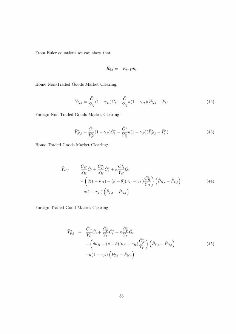
From Euler equations we can show that

R6;t = �Et�1mt

Home Non-Traded Goods Market Clearing:

bYN;t = �C�YN(1� H)Ct �

�C�YN�(1� H)( bPN;t � bPt) (42)

Foreign Non-Traded Goods Market Clearing:

bY �N;t = �C�

�Y �N(1� F )C�t �

�C�

�Y �N�(1� F )( bP �N;t � bP �t ) (43)

Home Traded Goods Market Clearing:

bYH;t =�CH�YHCt +

�C�H�YHC�t + �

�C�H�YHQt

���(1� �H)� (�� �)(�H � vF )

�C�H�YH

��PH;t � PF;t

�(44)

��(1� H)�PT;t � PN;t

�

Foreign Traded Good Market Clearing

bY �F;t =�CF�YFCt +

�C�F�YFC�t + �

�C�F�YFQt

����H � (�� �)(�F � vH)

�C�F�YF

��PF;t � PH;t

�(45)

��(1� H)�PT;t � PN;t

�

35

where Qt is the real exchange rate de�ned as:

Qt = P�t + St � Pt: (46)

It is possible to decompose the real exchange rate as follows:

Qt = (v � v�)Tt + (1� �)(P �N;t � P �T;t)� (1� )(PN;t � PT;t)

Home CPI:

Pt = H PT;t + (1� H)PN;t (47)

Home Traded Price Index:

PT;t = �H PH;t + (1� �H)PF;t (48)

Foreign CPI:

P �t = F P�T;t + (1� F )P �N;t (49)

Foreign Traded Price Index:

P �T;t = �F P�H;t + (1� �F )P �F;t (50)

Law of one price holds for imports:

PF;t = P �F;t + St (51)

P �H;t = PH;t � St (52)

Equity Prices:

36

VH;t � �EtVH;t+1 = �Ct � (PH;t � Pt)� �EtCt+1 + Et(PH;t+1 � Pt+1) (53)

+(1� �)Et(kH;t+1 + YH;t+1)

V �F;t � �EtV �F;t+1 = �Ct � (P �F;t + St � Pt)� �EtCt+1 (54)

+Et(P�F;t+1 + St+1 � Pt+1) + (1� �)Et(kF;t+1 + YF;t+1)

VN;t � �EtVN;t+1 = �Ct � (PN;t � Pt)� �EtCt+1 + Et(PN;t+1 � Pt+1) (55)

+(1� �)Et(kN;t+1 + YN;t+1)

V �N;t � �EtV �N;t+1 = �Ct � (P �N;t + St � Pt)� �EtCt+1 (56)

+Et(P�N;t+1 + St+1 � Pt+1) + (1� �)Et(k�N;t+1 + Y �N;t+1)

Realized Excess Returns:

Rx1;t = R1;t � R6;t = �(VH;t � Et�1VH;t) + (1� �)(kH;t + YH;t � Et�1kH;t � Et�1YH;t) (57)

+PH;t � Et�1PH;t

Rx2;t = R2;t � R6;t = �(V �F;t � Et�1V �F;t) + (1� �)(kF;t + Y �F;t � Et�1kF;t � Et�1Y �F;t) (58)

+P �F;t � Et�1P �F;t + St � Et�1St

Rx3;t = R3;t � R6;t = �(VN;t � Et�1VN;t) + (1� �)(kN;t + YN;t � Et�1kN;t � Et�1YN;t) (59)

+PN;t � Et�1PN;t

Rx4;t = R4;t � R6;t = �(V �N;t � Et�1V �N;t) + (1� �)(k�N;t + Y �N;t � Et�1k�N;t � Et�1Y �N;t) (60)

+P �N;t � Et�1P �N;t + St � Et�1St

Rx5;t = R5;t � R6;t = St � Et�1St (61)

The log-linearized model characterized by 23 equations from (38) to (61) involves the following

sequence of 25 variables:

37

fm; m�; C; C�; P ; P �; PH ; PF ; P�H ; P

�F ; PT ; P

�T ; PN ; P

�N ; St; Qt;

Rx1; Rx2; Rx3; Rx4; Rx5;t; VH ; V�F ; VN ; V

�N ; Wg

We close the model by either a domestic tradable price targeting rule, i.e. P �F;t = 0 and PH;t = 0;

or by a CPI targeting rule, i.e. P �t = 0 and Pt = 0

References

[1] Backus, David K. and Gregor W. Smith. 1993. "Consumption and Real Exchange Rates in

Dynamic Economies with Non-traded Goods." Journal of International Economics 35: 297-316.

[2] Backus, D. K., Kehoe, P. J. and Kydland, F. E., 1992. International real business cycles.

Journal of Political Economy 100 (4), 745-75.

[3] Baxter, Marianne; Urban J. Jermann; and Robert G. King, 1998, �Nontraded Goods, Non-

traded Factors, and International Non-Diversi�cation�. Journal of International Economics 44,

211-229.

[4] Benigno, G. and Thoenissen, C., 2007. "Consumption and Real Exchange rates with Incom-

plete Markets and Non-traded Goods". Journal of International Money and Finance (forth-

coming) .

[5] Benigno, P.,2007. "Portfolio Choices with Near rational Agents: A Solution of Some Interna-

tional Finance Puzzles", LUISS Guido Carli.

[6] Chari, V., Patrick Kehoe, Ellen McGrattan, 2002, "Can Sticky Price Models Generate Volatile

and Persistent Real Exchange Rates?. Review of Economic Studies 69(3):533-563

[7] Cole, Harold, and Maurice Obstfeld, 1991, �Commodity Trade and International Risk-Sharing:

How Much Do Financial Markets Matter?�. Journal of Monetary Economics 28, 3-24.

[8] Collard, Fabrice; Harris Dellas; Behzad Diba; and Alan Stockman, 2007, �Home Bias in Goods

and Assets,�manuscript, Toulouse School of Economics.

38

[9] Coeurdacier, Nicolas, and Pierre-Olivier Gourinchas, 2008, �When Bonds Matter: Home Bias

in Goods and Assets,�manuscript, London Business School.

[10] Coeurdacier, Nicolas; Robert Kollmann; and, Philippe Martin, 2007, �International Portfolios

with Supply, Demand, and Redistributive Shocks,�NBER working paper no. 13424.

[11] Coeurdacier, Nicolas; Robert Kollmann; and, Philippe Martin, 2008, �International Portfolios,

Capital Accumulation, and Portfolio Dynamics,�manuscript, London Business School.

[12] Corsetti, G., Dedola, L. and Leduc, S., 2008. International risk sharing and the transmission

of productivity shocks. The Review of Economic Studies 75: 443-473.

[13] Devereux, Michael B., and Alan Sutherland, 2006a, �Solving for Country Portfolios in Open

Economy Macro Models,�manuscript, Dept. of Economics, University of British Columbia.

[14] Devereux, Michael B., and Alan Sutherland, 2006b. �Financial Globalization and Monetary

Policy,�manuscript, Dept. of Economics, University of British Columbia.

[15] Engel, Charles, and Akito Matsumoto, 2007, �Portfolio Choice and Risk-Sharing in a Monetary

Open-Economy DSGE Model,�manuscript, Dept. of Economics, University of Wisconsin.

[16] Engel, Charles, and Akito Matsumoto, 2008, �International Risk-Sharing: Through Equities

or Bonds?�, manuscript, Dept. of Economics, University of Wisconsin.

[17] Evans, Martin D.D., and Viktoria Hnatkovska, 2007, �Solving General Equilibrium Models

with Incomplete Markets and Many Financial Assets,�manuscript, Dept.of Economics, Uni-

versity of British Columbia.

[18] Heathcote, Jonathan, and Fabrizio Perri, 2008, �The International Diversi�cation Puzzle is

Not as Bad as You Think,�manuscript, Dept. of Economics, University of Minnesota.

[19] Hnatkovska, Viktoria, 2005, "Home Bias and High Turnover: Dynamic Portfolio Choice with

Incomplete Markets", Dept. of Economics, University of British Columbia

39

[20] Lane, Philip R. and Gian Maria Milesi-Ferretti. 2001. "The External Wealth of Nations: Mea-

sures of Foreign Assets and Liabilities for Industrial and Developing Countries". Journal of

International Economics 55, 263-294.

[21] Lane, Philip R. and Gian Maria Milesi-Ferretti. 2006. "The External Wealth of Nations Mark

II: Revised and Extended Estimates of Foreign Assets and Liabilities, 1970-2004." IMF Work-

ing Paper WP/06/69 (March).

[22] Matsumoto, Akito, 2008, "The Role of Nonseparable Utility and Nontradables in International

Business Cycle and Portfolio Choice," manuscript, IMF.

[23] Obstfeld, Maurice, 2007, �International Risk Sharing and the Cost of Trade,�Ohlin Lectures,

Stockholm School of Economics.

[24] Sorensen, Bent E., Yi-Tsung Wu, Oved Yosha, and Yu Zhu. 2007. "Home Bias and Interna-

tional Risk Sharing: Twin Puzzles Separated at Birth". Journal of International Money and

Finance 26(4) :587-605

[25] Stockman, A.C. and Dellas,H., 1989, "International Portfolio Diversi�cation and Exchange

Rate Variability". Journal of International Economics 26: 271-290

[26] Stockman, A. C. and Tesar, L. L., 1995. Tastes and technology in a two-country model of

the business cycle: explaining international comovements. American Economic Review 85 (1),

168-85.

[27] Tille, Cedric, and Eric van Wincoop, 2007. �International Capital Flows,�manuscript, Dept.

of Economics, University of Virginia.

[28] Tille, Cedric, and Eric van Wincoop, 2008. �An Asset Pricing Model of International Capital

Flows,�manuscript, Dept. of Economics, University of Virginia.

[29] van Wincoop, Eric and Francis E. Warnock, 2006. "Is Home Bias in Assets Related to Home

Bias in Goods,?", Working Paper 12728, NBER.

40

Figure 1: Impulse response to domestic tradable endowment shock for the case with 2 nominalbonds & tradable PPI targeting under benchmark calibration

Figure 2: Impulse response to domestic tradable endowment shock for the case with 2 nominalbonds & CPI targeting under benchmark calibration

41

Figure 3: Sensitivity Analysis. Home bond position and cross-correlation between the real exchangerate and relative consumption for the case of 2 nominal bonds with CPI targeting for di¤erent valuesof relative variance of non-tradable to tradable endowment shocks

Figure 4: Sensitivity Analysis. Home bond position and cross-correlation between the real exchangerate and relative consumption for the case of 2 nominal bonds with CPI targeting for di¤erent valuesof �:

42

Figure 5: Sensitivity Analysis. Home bond position and cross-correlation between the real exchangerate and relative consumption for the case of 2 nominal bonds with CPI targeting for di¤erent valuesof �:

Figure 6: Impulse response to domestic tradable endowment shock for the case with 2 tradablesector equities under benchmark calibration

43

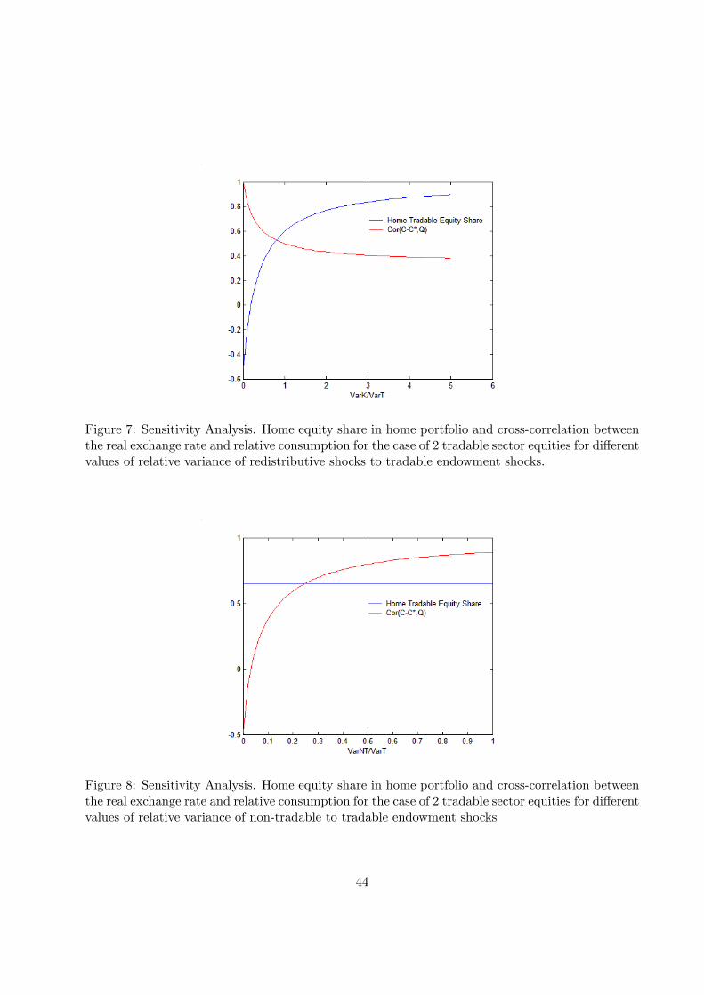
Figure 7: Sensitivity Analysis. Home equity share in home portfolio and cross-correlation betweenthe real exchange rate and relative consumption for the case of 2 tradable sector equities for di¤erentvalues of relative variance of redistributive shocks to tradable endowment shocks.

Figure 8: Sensitivity Analysis. Home equity share in home portfolio and cross-correlation betweenthe real exchange rate and relative consumption for the case of 2 tradable sector equities for di¤erentvalues of relative variance of non-tradable to tradable endowment shocks

44

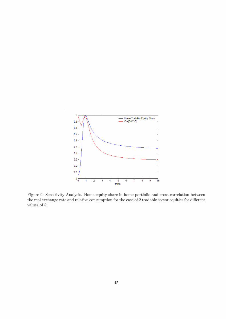
Figure 9: Sensitivity Analysis. Home equity share in home portfolio and cross-correlation betweenthe real exchange rate and relative consumption for the case of 2 tradable sector equities for di¤erentvalues of �:

45