Financial Intermediaries and International Risk Premia

Kyriakos Chousakos∗

October 2017

Abstract

I propose a measure of adjusted leverage as a proxy for the pricing kernel of a representative financialintermediary. Using a simple theoretical framework with information production, I show that in states ofthe world where credit outstanding in the economy is low, financial leverage is not an accurate proxy forthe stochastic discount factor of financial intermediaries. Empirical evidence confirms this theoreticalfinding for an international panel of financial intermediaries. Credit outstanding arises as an importantdeterminant of the stochastic discount factor of a financial intermediary. As a result, the new proposedmeasure incorporates information on both intermediaries’ financial leverage and the amount of credit inthe economy. It is an economically meaningful state variable that is pro-cyclical and predicts financialcrises. I show that a global adjusted leverage factor prices currency portfolios and global equity portfoliosoutperforming benchmark factor models designed to price these assets.

Keywords: Asset Pricing, International Financial Markets, Financial IntermediariesJEL Classification: G2, G12, G15, G24

∗Yale University. Email: kyriakos.chousakos@yale.edu. I am grateful to my advisors Gary Gorton, Tobias Moskowitz, andJonathan Ingersoll for their guidance and invaluable comments. I thank Oliver Boguth (discussant), Robin Greenwood, TylerMuir (discussant), and Guillermo Ordoñez for helpful comments and suggestions. I also thank Thomas Bonzcek, Arun Gupta,Toomas Laarits, Avner Langut, Adriana Robertson, and participants of the 5th Annual USC Marshall PhD Conference inFinance, the PhD Session of the 2017 Northern Finance Association Annual Conference, and the PanAgora 2017 Crowell PrizeSeminar Series for useful comments. All errors remain my own.

1 Introduction

Financial intermediaries are the primary participants in capital markets. In the foreign exchange market,

international commercial banks acting as securities dealers account for more than 51% of all transactions.1

In the equities market, over the past decades households have been steadily decreasing their direct stock

holdings, while financial intermediaries have been filling the void.2 In the bond market, almost all of the

trading takes place between broker-dealers and large institutional investors in over-the-counter markets.3

Financial intermediaries are sophisticated market participants that carry out complex trading strategies, face

low transactions costs, and continuously update their strategies as new information becomes available. As

a result, financial intermediaries are ideal candidates for the role of the marginal investor in a wide array

of markets which means that their marginal value of wealth is expected to price financial assets in these

markets.4

In this paper, I improve on existing intermediary asset pricing models and study the impact of financial

intermediaries on global capital markets. More specifically, shifting the focus from U.S. only to international

financial intermediaries, I propose and test an empirical proxy for the pricing kernel of a representative global

financial intermediary. This proxy in addition to financial leverage takes into account the amount of credit in

the economy. This is motivated by a simple theoretical framework with information production in which credit

outstanding in the economy along with financial leverage arises as an important determinant of the stochastic

discount factor (SDF) of financial intermediaries. Empirical evidence presented in the paper confirms this

theoretical finding. The proposed measure is an adjusted leverage index which incorporates information

on intermediaries’ financial leverage and the availability of credit in the economy. I show that adjusted

leverage is an economically meaningful state variable that is pro-cyclical and predicts financial crises and

future consumption levels. I find that a global adjusted leverage factor prices currency portfolios and global

equity portfolios outperforming benchmark factor models designed to price these assets. A decomposition of

the global adjusted leverage factor into non-U.S. and U.S. only components reveals that non-U.S. financial

intermediaries are marginal investors in foreign exchange markets as well as in global equity markets.

To motivate the empirical work of this paper, I develop a simple theoretical framework in the spirit

of Gorton and Ordoñez (2014) and Gorton and Ordoñez (2016). The economy comprises three agents –

firms, financial institutions, and households – all of which are risk neutral with respect to lending activities1See, the foreign exchange turnover section of the triennial central bank survey conducted by the Bank for International

Settlements (BIS) in September 2016 (www.bis.org/publ/rpfx16fx.pdf).2See, e.g. Allen (2001), and Sneider et al. (2013).3See, e.g. Edwards et al. (2007) for a breakdown of the percentage of bonds traded over-the-counter and in NYSE.4A growing stream of the literature, both theoretical and empirical, studies the relation between financial intermediaries and

asset prices. I discuss the different approaches in Section 2.

1

with the exception of financial institutions which are risk averse with regard to holding firms’ equity.5 To

produce output, firms need to borrow capital from households through the financial system posting land

as collateral. Both households and financial institutions may produce information regarding the quality of

the collateral backing deposits and loans respectively with the cost of producing information for households

being significantly higher compared to that for financial institutions.6 In this setting, information production

regulates the amount of credit outstanding and deposits in the economy. Both quantities are an increasing

function of expected output and their respective rates of increase depend on the current information production

regime.

In this framework, I show that the relation between the SDF, as described in the model by the marginal

value of wealth of a financial institution, and its financial leverage is not one-to-one and strongly depends on

the level of credit outstanding. An increase in financial leverage does not necessarily indicate a decrease in the

marginal value of wealth for the financial institution. This is primarily observed in times of economic growth,

where credit outstanding is high and financial intermediaries sustain high financial leverage and low marginal

value of wealth as a result of the ample investment opportunities which they can undertake. However, this

is not the case in times of recessions or financial crises, where the amount of credit outstanding is low. In

such times both financial leverage and the marginal value of wealth of a financial institution increase as a

result of an increase in deposits not followed by a similar increase in loans and profitability. According to the

theoretical framework discussed above, it is possible that in a low credit environment an increase in leverage

is associated with an increase in the marginal value of wealth of the financial institution. This implies that

financial leverage is not an accurate empirical proxy for the SDF of a financial intermediary. A number of

empirical findings, summarized below, corroborate this theoretical proposition.

Assets that co-vary with intermediaries’ SDF are riskier and investors require higher premia to compensate

for that risk. In the literature the SDF of financial intermediaries is proxied by leverage innovations of

financial intermediaries (see, e.g. Adrian et al. (2014)) or its reciprocal capital ratio innovations (see, e.g. He

et al. (forthcoming)). I empirically show that for an international panel of countries financial leverage interacts

differently with key characteristics of financial intermediaries, such as future financial assets and stock market

returns, depending on the level of credit outstanding in the economy. When the credit outstanding is high,

financial leverage is positively correlated with the level of future assets reflecting a higher risk bearing capacity

and negatively correlated with market returns indicating lower risk for such investments. On the other hand,5This assumption is primarily motivated by the third Basel Accord (Basel III) according to which secure debt is considered

to be more liquid than equity and as a result the capital requirements for financial institutions holding equities in their balancesheets are higher compared to these for secure debt assets.

6Financial institutions possess superior technology and resources in identifying the quality of collateral posted by firmscompared to that of households.

2

when the credit outstanding in the economy is low the opposite holds true. This finding suggests that a

potential proxy for the SDF of financial intermediaries ought to take into account credit outstanding in the

economy.

I construct a proxy for intermediaries’ SDF by combining information on financial leverage of broker-

dealers with information on economy-wide credit-to-private sector. More specifically, first, I compute a

measure of global financial leverage as the aggregated country level financial leverage weighted by the level of

financial assets of each country. Second, I compute a global measure of credit-to-private sector by aggregating

country level credit-to-private sector figures again weighted by the level of financial assets of each country.

Finally, the global adjusted leverage measure is equal to the negative global leverage innovations when global

credit is less than a threshold value and equal to global leverage innovations otherwise. The threshold is set

at the 25th percentile of a rolling window on the global credit series.

This adjusted leverage measure is directly related to business cycles. Consistent with theoretical and

empirical work suggesting that the marginal value of wealth of a financial intermediary is pro-cyclical (see, e.g.

Brunnermeier and Pedersen (2009) and Adrian and Shin (2010)), adjusted leverage is positively correlated with

changes in real GDP, capital formation, and total factor productivity (TFP) at a country level. In addition,

it predicts financial crises and future levels of durables and non-durables consumption. The relation between

adjusted leverage and business cycles implies that it is an economically meaningful measure summarizing

various aspects of economic activity related to financial intermediaries’ marginal value of wealth. Based on

these properties I argue that this measure can be employed as a reasonable proxy for the SDF of financial

intermediaries.

Using a single factor model, I perform cross-sectional asset pricing tests across a set of international asset

classes. I find that excess returns of currency portfolios and international equity portfolios can be explained

by their exposure to global adjusted leverage. More specifically, the global adjusted leverage factor appears

with a significantly positive price of risk consistently across all test assets. The global adjusted factor model

outperforms benchmark models (see, e.g. Lustig et al. (2011), Menkhoff et al. (2012a), and Menkhoff et al.

(2012b)) which aim to explain the cross-section of currency portfolios, and performs similarly to standard

multifactor models, such as the Fama-French global three factor plus momentum model, which aim to explain

the cross-section of international equity portfolios. The positive price of risk across asset classes is consistent

with the theoretical framework developed in this paper where assets that co-vary with intermediaries’ SDF

are associated with a higher risk premium. My findings suggest that the marginal value of wealth of financial

intermediaries is indeed an important determinant of asset prices.

3

A common criticism of cross-sectional asset pricing tests is that mis-estimated exposures (betas) in the

time-series regressions could be explaining a spurious relationship in the cross-section of returns (see, e.g.

Lewellen et al. (2010)). I address many of the concerns voiced in Lewellen et al. (2010) by conducting a

number of robustness checks. First, I estimate the exposures of test portfolios on the global leverage factor

and find that the adjusted leverage betas increase in a pattern consistent with an increasing adjusted leverage

being associated with higher premia. Second, I construct an adjusted leverage factor-mimicking portfolio and

repeat the asset pricing tests using a longer time-series. The price of risk of the global adjusted leverage

factor remains significantly positive across all test assets with the exception of momentum portfolios. Third,

I perform beta sorts to address the potential criticism that my results only hold for portfolios used in the

tests. I estimate the exposure of country-level market portfolios and country-level financial sector portfolios

on the adjusted leverage factor-mimicking portfolio and measure the spread in average returns of these

portfolios. The resulting spread is positive, suggesting that the adjusted leverage factor is truly priced in the

cross-section. Finally, for all cross-sectional asset pricing tests, I measure the fraction of instances where

a randomly generated factor achieves an explanatory power higher than and pricing error lower than that

generated by the global adjusted leverage factor. I find that for the majority of test assets this fraction is

extremely low (less than 1%).

A number of factors aiming to capture the marginal value of wealth of financial intermediaries have

been proposed in the literature. Adrian et al. (2014) propose a single-factor intermediary SDF. The factor is

a time-series of the shocks to the leverage of securities broker-dealers and carries a large and significantly

positive price of risk. On the other hand, He et al. (forthcoming) propose as a two-factor intermediary SDF.

The first factor is the market and the second is a time-series of the shocks to the equity capital ratio of primary

dealer counterparties of the New York Federal Reserve. Using an extensive set of test assets the authors show

that it carries a consistently positive price of risk. I compare the explanatory power of the global adjusted

leverage factor against that of the factors proposed by Adrian et al. (2014) and He et al. (forthcoming). I

find that the global adjusted leverage factor appears with a consistently positive price of risk across all test

assets and that it outperforms both the leverage factor and the capital factor in the cross-section currencies

and global equities. The better performance of the adjusted leverage factor as compared to that of other

factors proposed in the literature implies that this factor is a more accurate state variable reflecting global

financial intermediaries’ SDF.

This paper is organized as follows: Section 2 discusses the related literature and the contribution of the

paper; Section 3 develops a theoretical framework that motivates the empirical work; Section 4 presents the

data sources; Section 5 presents the construction of the adjusted leverage factor and discusses its properties;

4

Section 6 discusses the empirical methodology and how it relates to theory; Section 7 shows the main findings

of the paper; Section 8 revisits the empirical findings under alternative theoretical frameworks, compares the

performance of global adjusted leverage against other measures proposed in the literature, and decomposes

global adjusted leverage into a non-U.S. and a U.S. only component; and finally Section 9 concludes the

paper.

2 Related Literature and Contribution

This paper is closely related to two main streams of the literature.

First, a large stream of literature studies the relation between financial intermediaries and asset prices.7

Financial institutions are the class of investors whose characteristics most closely align with those of a

representative investor in traditional asset pricing models, and thus the study of their marginal value of wealth

is expected to provide a more instructive stochastic discount factor (SDF).8 Models of intermediary-based

asset pricing link the marginal value of wealth to intermediaries’ funding constraints implying that marginal

utility is high when funding constraints are binding (see, e.g. Brunnermeier and Pedersen (2009), Geanakoplos

(2010), Gromb and Vayanos (2002), and Shleifer and Vishny (1997)). A common theme across these models

is a pro-cyclical intermediary leverage, which implies a positive price of risk.9 In line with this stream of

research, Gabaix and Maggiori (2015) develop a model of exchange rate determination based on capital flows

in financial markets with frictions. Empirically, Adrian and Shin (2010) show that financial intermediaries

adjust their leverage actively according to economic conditions resulting in pro-cyclical leverage. Adrian

et al. (2014) and He et al. (forthcoming) show that shocks to the leverage and capital ratios of financial

intermediaries, respectively, explain a large portion of the cross-sectional variation in the expected returns of

an array of asset classes.10 Finally, DellaCorte et al. (2016a), focusing on the currency market, show that a

global imbalance risk factor (see, e.g. Gabaix and Maggiori (2015)) explains the cross-sectional variation in

currency excess returns.

The contribution of this paper to the financial intermediation literature is twofold. On the theory side,

I deviate from the intermediary-based asset pricing models mentioned above by introducing information7Financial intermediaries play a central role in modern markets. The importance of this role and the need for additional

research has been part of past AFA presidential addresses (see, e.g. Allen (2001), Duffie (2010), Cochrane (2011)).8This approach is in contrast to conventional consumption-based asset pricing models where the marginal investor is the

household (see, e.g. Campbell and Cochrane (1999) and Bansal and Yaron (2004)). Households exhibit limited stock marketparticipation (see, e.g. Vissing-Jørgensen (2002)), pay higher transactions costs, and exhibit a lack of financial sophistication(see, e.g. Calvet et al. (2007)).

9On the other hand, He and Krishnamurthy (2013) and Brunnermeier and Sannikov (2014) propose a central role forintermediaries’ wealth and generate a countercyclical intermediary leverage (negative price of risk).

10Etula (2013), Adrian et al. (2015), Adrian et al. (2013) show that the risk-bearing capacity of U.S. securities broker-dealersis a strong predictor of asset returns (commodities, currencies, equities, and bonds).

5

production by the agents in the economy as in Gorton and Ordoñez (2014) and Gorton and Ordoñez

(2016). More specifically, I propose an alternative mechanism where information production in the economy

determines the amount of credit outstanding in the economy and subsequently the level of financial leverage

and the SDF of financial intermediaries. On the empirical side, I expand the focus from U.S. to international

financial intermediaries, and propose and test the asset pricing properties of an empirical proxy for the

SDF of a global financial intermediary. This measure captures multiple aspects of economic activity ranging

from capital formation to financial crises and future consumption. The paper establishes an economically

meaningful link between the marginal value of wealth of a global financial intermediary and asset prices, thus

relating asset prices to the macroeconomy through the financial intermediaries’ pricing kernel. I deviate from

previously used methodologies in both the dimensions of variable construction and scope of test assets. The

measure of adjusted leverage is computed by aggregating granular (balance sheet) information in tandem

with information on credit-to-private sector from a wide array of countries. This method allows me to obtain

a more accurate representation of the SDF of financial institutions on a global level, since I combine two

pieces of information (balance sheet information and aggregate credit conditions), which leads to a greater

explanatory power over the cross-section of returns.11

Second, another large stream of literature studies international assets’ excess returns. The literature

around currency excess returns has focused on portfolio strategies based on currency characteristics, such as

the interest rate differential (carry trade (see, e.g. Hansen and Hodrick (1980), Meese and Rogoff (1983),

Fama (1984), Koijen et al. (2016))), past returns (momentum and value (see, e.g. Menkhoff et al. (2012b)

and Asness et al. (2013))), and global foreign exchange volatility. Explanations for currency premia include

aggregate consumption growth risk (see, e.g. Lustig and Verdelhan (2007)), currency crash risk and peso

problems (see, e.g. Brunnermeier et al. (2008), Burnside et al. (2011a) and Burnside et al. (2011b)), global

risk (see, e.g. Lustig et al. (2011)), habits (see, e.g. Verdelhan (2010)), and rare disasters (see, e.g. Farhi and

Gabaix (2016))12 The literature around international equity excess returns has focused on documenting the

existence of size, value, and momentum premia in equity markets across the world (see, e.g. Griffin (2002) and

Fama and French (2012)). Global versions of the Fama French three-factor model can explain a large part of

variation in international equity excess returns (see, e.g. Fama and French (2012)). Alternative explanatory

factors related to funding constraints of investors in international financial markets explain cross-country11Prior empirical research uses as proxies for the marginal value of wealth of financial intermediaries the changes in the

leverage ratio (see, e.g. Adrian et al. (2014)), or a measure of the intermediary capital ratio (see, e.g. He et al. (forthcoming)without taking into account the level of the available credit in the economy. The importance of high leverage or low availablecapital varies with respect to the available level of credit in the economy. The marginal utility of an intermediary when bothleverage and credit are high is not the same as when leverage is high and credit is low. In the second case the marginal utility ofan intermediary is higher.

12Additional explanations include the term structure (see, e.g. Bansal (1997), country-specific characteristics such as per-capitaGDP and inflation (see, e.g. Bansal and Dahlquist (2000)), currency volatility (see, e.g. Menkhoff et al. (2012a) and DellaCorteet al. (2016b)), downside risk CAPM (see, e.g. Lettau et al. (2014)), and global imbalances (see, e.g. DellaCorte et al. (2016a)).

6

variation in equity premia (see, e.g Goyenko and Sarkissian (2014) and Malkhozov et al. (2017)).

This paper contributes to the international finance literature and more specifically to the above mentioned

literature on risk factors associated with risk premia in currency and equity markets. I propose an alternative

explanation based on the role of financial intermediaries as marginal investors in these markets. This

explanation is based on an economically meaningful link between the marginal value of wealth of a global

financial institution and excess returns in the cross-section of currency and international equity portfolios.

3 Theoretical Framework

In this section, I develop a two period general equilibrium framework in the spirit of Gorton and Ordoñez

(2014) and Gorton and Ordoñez (2016).

3.1 Setting

The economy comprises three agents, each with a mass 1 – firms, financial institutions, and households –

and two types of goods – capital (numeraire) and land. All agents are risk neutral, apart from the financial

institutions which are risk neutral with regard to their lending activities and risk averse with regard to

holding firms’ equity. As in Gorton and Ordoñez (2014) only firms have access to managerial labor (L∗),

which combined with numeraire (K) produce more numeraire (K ′). The production process is stochastic

with Leontief technology:

K ′ =

A min{K,L∗} with prob. q

0 with prob. (1− q),

where A is a parameter determining output when production process is successful and q is the probability that

the production process is successful. For the purposes of this model I interpret q as the level of technological

innovation. A and q combined describe the efficiency of the production process.

Production is efficient (qA > 1) which means that the optimal amount of numeraire is K∗ = L∗. In this

economy, households begin with an endowment of numeraire K̄ > K∗ which can sustain optimal production.

Financial institutions are the sole owners of firm equity, which makes them the de-facto marginal investors.

Finally, firms own land and are endowed with numeraire in period 1 (K1) but have no means of capital

in period 2. Land is not used in production however it derives its value from the amount of numeraire it

7

produces at the end of the second period. If land is “good,” it yields C units of numeraire at the end of the

second period; if it is “bad,” it does not yield anything. Only a fraction p̂ of land is good.

In this economy, output and technological innovation (q) are non-verifiable, but the quality of land is not.

This makes land valuable as collateral. To receive capital necessary for production, firms pledge a fraction of

land as collateral for the loan they receive from the financial institution. This collateral is pledged in turn by

financial institutions to facilitate deposits from households. In this setting, C > K∗ which means that land

that is “good” can support the optimal capital size (K∗).

In period 1 the agents form beliefs about the fraction of land that is of good quality. To determine

the true quality of land with certainty, households must pay γh, while financial institutions must pay γb,

where γh > γb. This reflects the fact that financial institutions have superior technology compared to that of

households in determining the quality of collateral.

3.2 Optimal Loan for a Single Firm

Firms choose between debt that causes information production about the collateral leading to information-

sensitive debt, and debt that does not induce information production leading to information-insensitive debt.

Information acquisition for the financial institution bears a cost γb. As in Gorton and Ordoñez (2014), I

determine conditions under which debt is information-sensitive or information-insensitive.

3.2.1 Information-Sensitive Debt

In this case, financial institutions discover the true value of the firms’ land at a cost γb. Financial

institutions are risk neutral when it comes to their lending activity which means that they break even:

p(qRbIS + (1− q)xbISCf −Kb) = γb, (1)

where Kb is the actual loan from the financial institution to the firm, RbIS is the face value of the debt, and

xbIS is the fraction of land posted as collateral.

The fraction of collateral that a firm posts is determined by,

RbIS = xbISCf ⇒ xbIS = pKb + γb

pCf.13

13If RbIS > xbISCf , the firm would always hand over the collateral instead of repaying the loan. On the other hand, if

8

Expected profits (net of land value) are

E(π|p, IS) = p(qAKb − xbISCf ) = pK∗(qA− 1)− γb.14 (2)

3.2.2 Information-Insensitive Debt

In this case, financial institutions do not produce information regarding the quality of firms’ land. As

financial institutions are risk neutral with respect to their lending activity and break even,

qRbII + (1− q)pxbIICf = Kb, (3)

where RbII = pxbIICf as with the previous case.

Financial institutions could potentially deviate and privately check the quality of the land prior to

lending capital. The following condition guarantees that they will not deviate since the expected payoff from

producing information is less than the cost (γb):

p(qRbII + (1− q)xbIICf −Kb) < γb ⇒ (1− p)(1− q)Kb < γb.

The financial institution lends the optimal amount of capital (K∗) if the above condition is satisfied for

Kb = K∗. However, if the above condition is not satisfied, the amount of capital is Kb = γb

(1−p)(1−q) or pCf ,

if collateral value is low. Combining the above, the loan level for information-insensitive debt is:

Kb(p, q|II) = min

{K∗,

γb

(1− p)(1− q) , pCf

}. (4)

Expected profits (net of land value) are

E(π|p, II) = pqAKb − xbIIpCf = K(p, q|II)(qA− 1). (5)

Equating profits under information-sensitive debt (equation 2) with profits under information-insensitive

debt (equation 5) allows to pin down the level of the loan under information-sensitive debt:

RbIS < xbISCf the firm would always sell the collateral and repay the loan. This means that RbIS = xbISC

f .14I assume that it is feasible to borrow the optimal amount of capital (K∗), which means that xbIS = pKb+γb

pCf ≤ 1 and thatpK∗(qA− 1) > γb. Combining the two yields the condition qA < Cf/K∗.

9

Kb(p, q|IS) = pK∗ − γb

qA− 1 . (6)

3.3 Optimal Deposits for a Financial Institution

In this setting the owners of capital are households, which deposit their wealth in financial institutions,

which in their turn lend it to firms. The banks choose between deposits that cause information production

about the ability of the bank to repay, and deposits that do not induce information production. Both banks

and households make their decisions simultaneously which means that the household cannot infer the quality

of collateral from observing the bank’s loan. The creditworthiness of the financial institution is determined by

the amount of collateral that the firm has pledged for the loan it received. The cost of information acquisition

for the household is γh.

3.3.1 Information-Sensitive Deposits

In this case, households discover the true value of the financial institution’s loans, backed by firms’ land

as collateral, by incurring the cost γh. Households are risk neutral and break even:

p(qRhIS + (1− q)xhISCb −Kh) = γh (7)

where Kh is the actual amount of deposits in the financial institution, RhIS is the face value of deposits, and

xhIS is the fraction of the financial institution’s loans posted as collateral. For the same reason as before, the

fraction of collateral that the financial institution posts is xbIS = pKh+γh

pCb . Since the collateral posted by the

financial institution is the land that has been posted by the firm to obtain its loan, Cb = Cf .

Expected profits for the financial institution are

E(πb|p, IS) = pxbISCf − pxhISCb = pKb + γb − pKh − γh.15 (8)

3.3.2 Information-Insensitive Deposits

In this contract, financial institutions attract deposits without triggering production of information

regarding their assets. Since households are risk neutral and break even:15Because of the assumption that γh > γb the bank will always produce information before the household does as both q and

p decline.

10

qRhII + (1− q)pxhIICb = Kh, (9)

where RhII = pxhIICb for the same reasons as before, which means that xhII = pKh+γh

pCb .

For the contract to be information-insensitive, no household should have an incentive to deviate. This is

guaranteed by:

p(qRhII + (1− q)xhIICb −Kh) < γh ⇒ (1− p)(1− q)Kh < γh.

As with the information-sensitive loan to the firm, the deposits contract will reach the optimal amount

of capital (K∗) if the above condition is satisfied. If it is not, the amount of deposits will either be

Kh = γh

(1−p)(1−q) , if the financial institution faces credit constraints, or pCb if the collateral value is low. Thus,

Kh(p, q|II) = min

{K∗,

γh

(1− p)(1− q) , pCb

}. (10)

Expected profits for the financial institution are

E(πb|p, II) = pxbIICf − pxhIICb = Kb −Kh. (11)

Equating profits under information-sensitive deposits (equation 8) with profits under information-

insensitive deposits (equation 11) allows to pin down the level of deposits under information-sensitive

debt:

Kh(p, q|IS) = (1− p)KbIS + γh − γb

1− p . (12)

Figure 1a shows the amount of credit in the form of deposits and loans that the household and the

financial institution respectively are willing to make depending on the probability of success of the production

process (q) keeping the fraction of land that is good (p) constant. For the remainder of this section, this

probability will represent technological innovation. The cutoffs in Figure 1a are determined as follows:

Cutoff A occurs at the level of technological innovation below which firms reduce their borrowing so that

they do not induce information production. From above:

11

K∗ = γb

(1− p)(1− q) ⇒ qb,HII = 1− γb

K∗(1− p) . (13)

Cutoff B is determined by the level of technological innovation below which financial institutions reduce

their deposits thus avoiding information production from households. As before:

K∗ = γh

(1− p)(1− q) ⇒ qh,HII = 1− γh

K∗(1− p) . (14)

Cutoff C is obtained after equalizing information-sensitive debt with information-insensitive debt:

γb

(1− p)(1− q) = pK∗ − γb

(qA− 1) . (15)

The positive root of the above quadratic equation (qbIS) is the level of technological innovation below which

financial institutions acquire information about the quality of land that firms post as collateral for their loan.

Cutoff D is obtained similarly for the case of deposits,

γh

(1− p)(1− q) = pK∗ − γb

(qA− 1) + γb − γh

(p− 1) . (16)

The above cutoffs create four distinct regions: (1) Between A and B (B(II), H(II)), both the bank and the

household are information-insensitive (II). Also, bank credit is constrained and firms cannot borrow without

triggering information production, which means that credit rationing takes place in bank lending; (2) Between

B and C (B(II), H(II)), both agents are information-insensitive (II) but credit constraints lead to rationing

in both bank lending and deposits; (3) Between C and D (B(IS), H(II)), the bank is information-sensitive

(IS) and at a cost γb discovers the true value of the land. The household is still information-insensitive and

rationing takes place in deposits; and (4) Below D (B(IS), H(II)), both agents are information-insensitive

with banks producing information about the quality of land and households producing information about the

quality of the assets of the financial institution.16

The amount of credit that is available in the economy to fund firms’ projects is a function of technological

innovation (q), the quality of land (p), and the cost of information production for financial institutions (γb)

and households (γh). For the purposes of this paper, I assume that the quality of land and the cost of16Additional regions become relevant depending on the level of the fraction of land that is good p and the value C of land.

Low collateral value can constrain the amount of deposits and subsequent loan amount, however for high enough levels of p, itbecomes irrelevant.

12

information acquisition remain constant throughout the two periods. Proposition 1 summarizes the relation

between technological innovation and the amount of credit in the economy. The proof is trivial.

Proposition 1. (Effect of technological innovation on credit.)

For fixed values of γb, γh, and p, with γb < γh and K∗ < pCf = pCb:

• Deposits are an increasing function of technological innovation (q) for q < qh,HII and independent of q

otherwise.

• Loans are an increasing function of technological innovation (q) for q < qb,HII and independent of q

otherwise.

3.4 Firm Valuation

As mentioned above, in this economy the financial institutions are the sole owners of firms. They are

risk averse with respect to their equity holdings and risk neutral with respect to their lending activity. This

assumption is motivated primarily by current banking regulation which mandates bank capital requirements

and determines internal risk-management policies. More specifically, according to the Third Basel Accord

(Basel III) equities are deemed substantially less liquid than high quality corporate debt. This means that

equities in intermediaries’ balance sheets require a higher capital provision compared to that required for high

quality corporate debt.17 I derive the stochastic discount factor (SDF) and compute the financial leverage of

financial institutions in a two period general equilibrium framework. Table 1 summarizes the timeline for this

economy. The financial institution maximizes a logarithmic utility function with two terms, a deterministic

component for the first period and a stochastic component for the second period,

max{Ct}2

t=1

Eu(C1, C2) = log(C1) + βElog(C2) (17)

Subject to:

C1 +Kb + γb + V1a1 = (π1(q1) + V1)a0 +Kh (18)

and

Kh + C2 = Kb + π2(q)a1 + pCf (19)17Basel III requires financial institutions and non-bank financial companies deemed systemically important to have enough

high-quality liquid assets (HQLA) which can be quickly liquidated to meet possible future liquidity needs. Assets are classifiedinto three groups (Level 1, Level 2A, and Level 2B) according to their liquidity properties. A total HQLA is computed as theweighted sum of the the asset value times a weight that is consistent with its liquidity group. Haircuts vary from 0% for assets inLevel 1 to 50% for assets in Level 2B. Common equity falls into Level 2B and is subject to a 50% haircut which is significantlyhigher compared to the 15% haircut of high quality (>AA- rating) corporate debt (see, e.g. www.bis.org/publ/bcbs238.pdfand www.bis.org/bcbs/publ/d406.pdf).

13

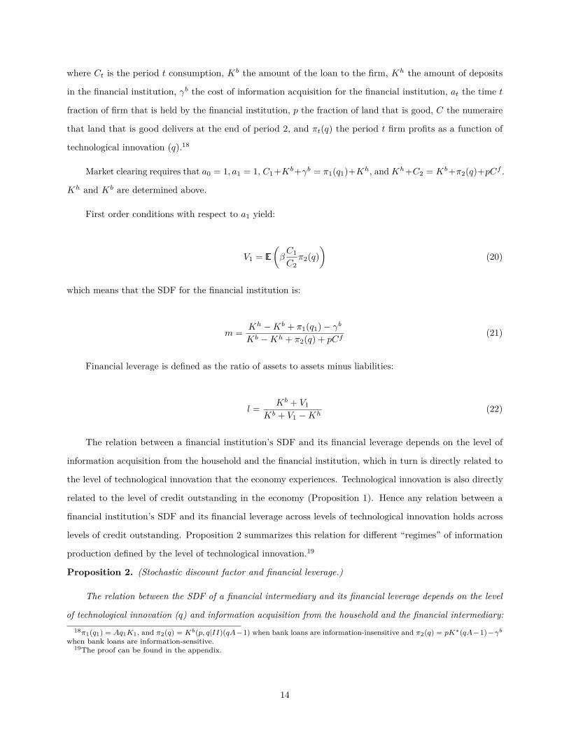
where Ct is the period t consumption, Kb the amount of the loan to the firm, Kh the amount of deposits

in the financial institution, γb the cost of information acquisition for the financial institution, at the time t

fraction of firm that is held by the financial institution, p the fraction of land that is good, C the numeraire

that land that is good delivers at the end of period 2, and πt(q) the period t firm profits as a function of

technological innovation (q).18

Market clearing requires that a0 = 1, a1 = 1, C1+Kb+γb = π1(q1)+Kh, andKh+C2 = Kb+π2(q)+pCf .

Kh and Kb are determined above.

First order conditions with respect to a1 yield:

V1 = E

(βC1

C2π2(q)

)(20)

which means that the SDF for the financial institution is:

m = Kh −Kb + π1(q1)− γb

Kb −Kh + π2(q) + pCf(21)

Financial leverage is defined as the ratio of assets to assets minus liabilities:

l = Kb + V1

Kb + V1 −Kh(22)

The relation between a financial institution’s SDF and its financial leverage depends on the level of

information acquisition from the household and the financial institution, which in turn is directly related to

the level of technological innovation that the economy experiences. Technological innovation is also directly

related to the level of credit outstanding in the economy (Proposition 1). Hence any relation between a

financial institution’s SDF and its financial leverage across levels of technological innovation holds across

levels of credit outstanding. Proposition 2 summarizes this relation for different “regimes” of information

production defined by the level of technological innovation.19

Proposition 2. (Stochastic discount factor and financial leverage.)

The relation between the SDF of a financial intermediary and its financial leverage depends on the level

of technological innovation (q) and information acquisition from the household and the financial intermediary:18π1(q1) = Aq1K1, and π2(q) = Kb(p, q|II)(qA−1) when bank loans are information-insensitive and π2(q) = pK∗(qA−1)−γb

when bank loans are information-sensitive.19The proof can be found in the appendix.

14

• Bank loans and household deposits are information-insensitive with no credit constraints present (B(II),

H(II)): Leverage is constant and SDF a negative function of technological innovation.

• Bank loans and household deposits are information-insensitive, but credit constraints are present (B(II),

H(II)): Leverage is positively and SDF negatively correlated with technological innovation.

• Bank loans and household deposits are information-insensitive, but deposit and credit constraints are

present (B(II), H(II)): Leverage is positively and SDF negatively correlated with technological innovation.

• Bank loans are information-sensitive and household deposits are information-insensitive with deposit

constraints present (B(IS), H(II)): Both leverage and SDF a positive function of technological innovation

• Bank loans and household deposits are information-sensitive (B(IS), H(IS)): Leverage is positively and

SDF negatively correlated with technological innovation.

Figure 1b provides an illustration of Proposition 2. For a high level of technological innovation and

credit outstanding, the relationship between SDF and financial leverage is negative. An increase in financial

leverage is associated with a decrease in the SDF of the financial institution. This usually represents times

of economic growth where the financial institution is able to sustain a relatively high level of leverage due

to the availability of a large number of profitable investment opportunities and the high level of funding it

secures from the household. However, when technological innovation and credit outstanding is at a relatively

low level and the household does not yet produce information, the relationship between the two variables is

the opposite.20 An increase in financial leverage is associated with an increase in the SDF of the financial

institution. The change in the relationship between the two variables is caused by the fact that the rate of

increase in deposits is higher than that in loans and the valuation of the firm. The increase in funding from

households does not keep up with the improvement in the profitability of investment opportunities in the

economy leading to an increasing leverage ratio and an increasing SDF. This usually represents times of

economic recession or financial crises where the financial institution may have sufficient funding, but not

enough investment opportunities leading to high levels of leverage.

Both Proposition 2 and Figure 1b underline the point that financial leverage is not always an accurate

measure of the SDF of a financial institution. In times when credit is low the relation between the two

variables reverses and a more accurate proxy of the marginal value of wealth of financial institutions should

take that into account. When credit is high, assets that co-vary with leverage are riskier and as a result

should earn higher premia. On the other hand, when credit is low, assets that co-vary with leverage are less20Usually the household does not produce information about the quality of the assets of the financial institution, unless there

is widespread uncertainty about the health of the financial system. Which makes the last case of Proposition 2 less likely to beobserved in the data.

15

risky and should earn lower premia.21 In the following section, I propose an empirical measure that takes

this point directly into account and combines information from both credit and financial leverage.

4 Data

This section describes the data used in the empirical analysis. I provide details on the construction of

the adjusted leverage factor, currency excess returns, currency portfolios, and the macroeconomic variables

used in the empirical tests.

4.1 Leverage Ratio

Intermediary asset pricing models suggest that financial intermediaries are sophisticated investors who

play a leading role in capital markets. They are considered marginal investors which means that their pricing

kernel is relevant for pricing the cross-section of risky assets.22 Motivated by the theoretical framework

developed above, I construct a proxy for the marginal value of wealth which takes into account the leverage

ratios of financial intermediaries and the credit conditions in the economy. I compute leverage ratios for

financial institutions that act as broker-dealers for an international panel (Table 2) using data from Thomson

Reuters WorldScope.23 I delete duplicate entries and data on ADRs. Leverage ratios are computed as follows:

Leverage = log

(Assets

Assets− Liabilities

)(23)

4.2 Assets Portfolios

For the purposes of the asset pricing tests of Section 7.1 I use currency and global equity portfolios.

I construct six forward discount portfolios following the methodology of Lustig et al. (2011). I rank21This relation can reverse if financial institutions face a higher cost of information acquisition on the firms’ assets than

households do (γb > γh). However, this does not seem to be the case in modern economies where financial institutions have aplethora of resources at their disposal to research and identify the quality of the posted collateral.

22There are two approaches to modeling an intermediary pricing kernel each of which has a different theoretical motivation.The first uses intermediary leverage as a proxy for the SDF (see, e.g. Brunnermeier and Pedersen (2009), while the second usesintermediary wealth (see, e.g. He and Krishnamurthy (2013) and Brunnermeier and Sannikov (2014)). Throughout this paper Ifollow the first approach.

23The actual WorldScope industry codes for financial firms used in the analysis are: 4310 for Commercial Banks - Multi-BankHolding Companies (used only for international financial institutions), 4394 for Securities Brokerage Firms, and 4395 forMiscellaneous Financial. Financial institutions classified as commercial banks in the database serve as broker-dealers in manycountries. Commercial Banks - Multi-Bank Holding Companies (4310, U.S only data), Commercial Banks - One Bank HoldingCompanies (4320), Investment Companies (4350), Commercial Finance Companies (4360), Insurance Companies (4370), Landand Real Estate (4380), Personal Loan Company (4390), Real Estate Investment Trust Companies, including Business Trusts(4391), Rental & Leasing (4392), and Savings & Loan Holding Companies (4393) are not included.

16

currencies from low to high interest rates such that portfolio 1 contains currencies with the lowest forward

discounts, and portfolio 6 contains the currencies with the highest forward discounts. The strategy that is

long on portfolio 6 and short on portfolio 1 represents carry trade and constitutes the carry factor (CAR)

that I use in the following asset pricing tests. Currency momentum portfolios are constructed using the

methodology of Menkhoff et al. (2012b). Each month I form six portfolios on the basis of excess currency

returns of the previous n months. Portfolio 1 contains currencies with the lowest prior n month returns,

while portfolio 6 comprises of currencies with the highest prior n month returns. I construct two types of

momentum portfolios, long-term momentum (n = 12 months) and short-term momentum (n = 1 month). The

strategy that is long on short-term momentum portfolio 6 and short on portfolio 1 constitutes the momentum

factor (MOM). I construct value portfolios following the methodology in Asness et al. (2013). As with

currency momentum, I form six portfolios based on the lagged five-year excess return of the currency of

each country in the sample. I assign the lowest lagged returns to portfolio 1 and the highest to portfolio 6.

Global equities portfolios comprise twenty-five international size and value sorted portfolios and the

twenty-five international size and momentum portfolios all obtained from Kenneth French’s online

data library.24

4.3 Macroeconomic Data

In Section 5, I explore the properties of the adjusted leverage measure with respect to macroeconomic

variables. Annual Real GDP and capital formation are from the Penn World Tables (PWT), domestic credit

to private sector, credit to households and credit to corporates are from the World Bank World Development

Indicators. Financial crisis episodes are from Valencia and Laeven (2012). Global imbalances are defined

as the difference between assets and liabilities denominated in the same currency. I construct the measure

of total global imbalances, which is the sum of global imbalances issued in domestic and foreign currency

standardized for the GDP of a country. For additional details see Bénétrix et al. (2015).25 Market returns are

the average market returns at a country level, financial intermediaries returns are the average financial sector

returns at a country level, and global volatility is the average market volatility among an international set of

countries (see, e.g. Chousakos et al. (2016)). In addition, and only for the U.S. economy, I collect data on

credit spreads, per capita consumption on durables, non-durables, and private investment from the Federal

Reserve Economic Data (FRED) maintained by the St. Louis FED. Table 3 summarizes the data used in this

paper.24http://mba.tuck.dartmouth.edu/pages/faculty/ken.french/data_library.html#International.25The dataset can be found at Philip Lane’s website http://www.philiplane.org/BLSJIE2015data.htm.

17

5 Adjusted Leverage

In the literature the marginal value of wealth of financial institutions is proxied by their financial leverage

and more specifically by seasonally adjusted changes in the level of broker-dealer leverage (see, e.g. Adrian et

al. (2014)). This could be potentially problematic because as discussed in Section 3 financial leverage or its

reciprocal capital ratio does not fully characterize the risk-bearing capacity of financial intermediaries across

all states of the economy. An increase in financial leverage does not necessarily indicate a decrease in the

marginal value of wealth for the financial institution. This could be true in times of economic growth, where

credit outstanding is high and the financial system can sustain high levels of leverage as financial intermediaries

are able to pursue profitable investments and at the same time raise capital if needed. However, this is not

the case in times of recessions or financial crises, where the amount of credit outstanding is low. According

to the theoretical framework discussed above, it possible that in a low credit environment an increase in

leverage is associated with an increase in the marginal value of wealth of the financial institution due to a

lack of profitable investment opportunities. A number of empirical findings, summarized below, suggest that

financial leverage interacts differently with key characteristics of financial intermediaries depending on the

level of credit outstanding in the economy.

The level of assets of financial intermediaries reflects among other factors their risk-bearing capacity.

A high level of assets in intermediaries’ balance sheets is usually the result of higher risk-bearing capacity.

If the financial leverage of an intermediary is a good proxy for its risk-bearing capacity, then the relation

between leverage and the level of future assets is expected to be positive across all states of the economy (see

e.g. Adrian et al. (2014)). The following regression specification provides a test of the above claim:

assetsn,t+q = αn + αt+q + β′Xn,t + γassetsn,t + εn,t+q (24)

where assetsn,t+q is the logarithm of the financial assets of country n at time t + q quarters, Xn,t =

(fin.leveragen,t, fin.leveragen,t × 1(Creditn,t > 75%), fin.leverage× 1(Creditt < 25%))′, fin.leveragen,t

is the logarithm of financial leverage of country n at time t, 1(Creditn,t > 75%) is a dummy variable

representing instances where credit-to-private sector of a given country is higher than the 75th percentile

of the cross-section of credit outstanding values at a given time, 1(Creditn,t < 25%) is a dummy variable

representing instances where credit-to-private sector of a given country is lower than the 25th percentile of

the cross-section of credit outstanding values at a given time, αn represents country fixed effects, and αt+q

time fixed effects.

18

Table 4 shows that the relation between leverage and the level of future assets is not consistently positive

across all states of the economy for an international panel of financial institutions aggregated at the country

level. More specifically, when interacted with the dummy variable 1(Creditn,t > 75%), and the dummy

variable 1(Creditt < 25%), the relationship between financial leverage and future assets is not consistently

positive. In the first case, financial leverage and future levels of assets are positively correlated, suggesting a

higher risk-bearing capacity, while in the second case a negative correlation suggests a lower risk-bearing

capacity leading to lower future levels of assets.26 Figure 2 confirms the above findings using country level

time-series regressions. When credit is low compared to the historical credit series for the country, the

majority of countries exhibits a negative correlation between leverage and future levels of assets, while the

opposite holds true when credit is high.

Another variable that reflects the risk-bearing capacity of financial institutions is intermediaries’ future

stock returns. According to traditional finance theory, higher expected returns usually reflect riskier

investments. Financial intermediaries that are perceived to be riskier usually face tighter funding constraints

and their risk-bearing capacity is limited. To test this claim I repeat the previous exercise, but now I replace

future assets with future returns. The regression specification is as follows:

rfinn,t+q = αn + αt+q + β′Xn,t + γrfinn,t + εn,t+q (25)

where rfinn,t+q is the logarithm of the market returns of financial intermediaries of country n at time t + q

quarters. Table 5 shows that on an aggregate level, financial intermediaries with high financial leverage

operating in a high credit environment consistently earn lower returns, while similar financial institutions

operating in a low credit environment earn consistently higher returns. This finding suggests that financial

leverage alone does not fully capture intermediaries’ risk-bearing capacity. Financial leverage viewed in

tandem with credit-to-private sector can be considered as a more accurate proxy for the marginal value of

wealth of financial intermediaries.27 As with the case of future assets, Figure 3 confirms the panel regression

findings using country level time-series regressions.

Motivated by the above findings, I propose a measure of a global adjusted leverage, which in addition to

financial leverage takes into account the level of credit-to-private sector at a global level. This measure serves

as a proxy for the marginal value of wealth of financial intermediaries and it is used in the asset pricing

tests of Section 7. I construct the global adjusted leverage index as follows: First, I compute a measure of26The same pattern holds true when focusing only on the U.S. economy (table can be found at the internet appendix).27The same pattern holds true when focusing only on the U.S. economy (Table can be found at the accompanying internet

appendix).

19

global financial leverage (Figure 4a) as the aggregated country level financial leverage weighted by the level

of financial assets of each country,

Global Leveraget =N∑c=1

wc,tLeveragec,t

where Leveragec,t is the country level financial leverage computed by aggregating firm level financial leverage,

wc,t = Assetsc,t∑N

c=1Assetsc,t

, and Assetsc,t =∑Mi=1 Assetsc,i,t. Second, I compute a global measure of credit-to-

private sector (Figure 4b) by aggregating the country level credit-to-private sector again weighted by the

level of financial assets of each country,

Global Creditt =N∑c=1

wc,tCreditc,t

Finally, the global adjusted leverage measure is equal to the residuals of an AR(1) process on global leverage

when credit-to-private sector is higher than the 25th percentile of a 12 quarter rolling window and equal

to the negative residuals of the same AR(1) process when credit-to-private sector is lower than the 25th

percentile of a 12 quarter rolling window (Figure 4c).28 The AR(1) process is,

Global Leveraget = α+ βGlobal Leveraget−1 + εt

The Adjusted leverage measure is,

Adjusted Leveraget =

−ε̂t if 1(Credit < 25th Percentile) = 1

+ε̂t otherwise.(26)

The rolling window guarantees no forward looking bias in the computation of the measure. Figure 5 shows

how the global adjusted leverage measure compares to innovations in global financial leverage. The correlation

between the two measures is 52.9%.

The risk-bearing capacity of financial intermediaries is associated with the state of the macroeconomy. It

is pro-cyclical, which suggests that favorable funding conditions are usually observed in periods with higher

credit outstanding, capital formation, and aggregate output. Adjusted leverage as a proxy for intermediaries’

risk-bearing capacity is expected to exhibit such a pro-cyclical behavior. Using an international panel28An alternative way to derive the adjusted leverage measure would be to compute the residuals of an AR(1) process on the

product of leverage and credit-to-private sector. In results which are available upon request, I show that this alternative adjustedleverage measure shares most of the properties of the adjusted leverage measure discussed above, however the explanatory powerof the second is significantly higher.

20

of observations, I perform a set of country level regressions of macroeconomic variables on the adjusted

leverage measure. Figures 6 and 7 summarize the results. Adjusted leverage is positively correlated with

contemporaneous changes in real GDP, capital formation, total factor productivity (TFP), and future financial

assets. This finding confirms that adjusted leverage is a pro-cyclical measure. In addition, adjusted leverage

is positively correlated with contemporaneous changes in credit to households, while the opposite holds true

for the case of credit-to-corporate entities. An increase in the global risk-bearing capacity is immediately

reflected in credit-to-households, but not in credit-to-corporate entities possibly due to the fact that corporate

loans require a longer assessment period. Total global imbalances are, in general, negatively correlated with

adjusted leverage suggesting that an increase in the global risk-bearing capacity of financial institutions leads

to a net loss of capital to advanced countries such as the U.S., France, and Denmark.29

The adjusted leverage measure incorporates, by construction, information about credit conditions in

the economy. Schularick and Taylor (2012) document that credit growth is a strong predictor of financial

crises. This finding motivates the following tests of the predictive power of adjusted leverage over financial

crises. Using an international panel, I regress the occurrence of a financial crisis on a set of lagged adjusted

leverage observations. I employ both a linear probability model and a logistic regression specification. Table

7 shows that 6-month lagged observations of adjusted leverage negatively predict financial crises. This finding

suggests that, prior to financial crises, financial institutions exhibit a lower risk-bearing capacity. This lower

risk-bearing capacity suggests that financial institutions could potentially adjust their activity to better

prepare themselves for an imminent financial crisis.

The U.S economy is no exception to the above mentioned patterns presented in Figures 6 and 7. Global

adjusted leverage is a pro-cyclical measure, positively correlated to changes in credit-to-households, real

GDP, capital formation, and TFP, while negatively correlated with the occurrence of financial crises and

credit spreads. Figure 8 looks at the relation between adjusted leverage, future per-capita consumption, and

future private investments on an expanding window reaching five years into the future. More specifically,

an increase in adjusted leverage is associated with a short term (1-year) increase in per-capita consumption

both in durables and non-durables, while an increase in adjusted leverage is associated with a medium term

(4,5-year) increase in private investments. This finding further supports the pro-cyclical nature of adjusted

leverage and shows that an increase in the risk-bearing capacity of the financial sector leads to an increase in

lending activity, both in the short- and in the long-term.

From the above findings, I conclude that adjusted leverage can be used as a reasonable proxy for the

marginal value of wealth of a financial intermediary. Adjusted leverage is high when credit conditions are29And possibly to other countries not in the current sample of countries.

21

favorable and low when credit conditions are adverse and leverage is high. It is pro-cyclical (positively

correlated with other measures of credit, real GDP, capital formation, and TFP), which is a characteristic of

marginal value of wealth that is consistent with theory (see, e.g. Brunnermeier and Pedersen (2009)), predicts

financial crises, and correlates with future consumption of durables and non-durables. The pro-cyclical nature

of adjusted leverage implies that this measure increases in good times when funding constraints are lax. In

the following sections, I test the asset pricing properties of this measure for both currency and global equity

portfolios.

6 Adjusted Leverage Factor in an Asset Pricing Setting

In this section I propose a pricing model which attempts to more accurately capture financial intermedi-

aries’ marginal value of wealth. I discuss how it relates to the theoretical framework of Section 3 and describe

the empirical methodology used to test its asset pricing properties.

6.1 Adjusted Leverage as Stochastic Discount Factor

In Section 3, I derived the stochastic discount factor of a financial institution in a two period economy

and discussed its relation with financial leverage across different levels of credit outstanding and technological

innovation, which define a set of information production regimes. More specifically, I show that when

both loans and deposits are information-insensitive, the relation between the stochastic discount factor

of the financial institution and financial leverage is negative, with the first decreasing while the second

increasing as credit outstanding in the economy increases. These information production regimes occur

when credit outstanding and technological innovation in the economy are at a relatively high level. The

increase in financial leverage is associated with a decrease in the marginal value of wealth of the financial

institution mainly due to the increase in the profitability of the firm. On the other hand, when loans are

information-sensitive and deposits are information-insensitive, the relation between the stochastic discount

factor of the financial institution and financial leverage is positive. This information production regime occurs

when credit outstanding and technological innovation are at relatively low levels. Both measures increase as

credit increases due to the fact that the increase in deposits is higher than that of the profitability of the firm.

This means that if SDFt ≈ α− bcLeveraget, then when credit is sufficiently high, assets that co-vary

with leverage are risky and earn a higher risk premium (bc > 0), while when credit is sufficiently low, assets

that co-vary with leverage are less risky and earn a lower risk premium (bc < 0). The proposed global adjusted

22

leverage measure addresses exactly this point by incorporating information from both credit outstanding

and financial leverage. Hence, SDFt ≈ a− b ·Adjusted Leveraget. In Section 7 I discuss the asset pricing

properties of adjusted leverage and show how consistent these properties are with this theoretical framework.

6.2 Empirical Methodology

In this section, I propose a linear factor model which consists of the global adjusted leverage factor. Using

a cross-section of asset returns, I test for the asset pricing properties of this factor using the methodology

proposed by Lewellen et al. (2010). The proposed SDF is linear in the global adjusted leverage factor:

SDFt = 1− b ·Adjusted Leveraget (27)

In the absence of arbitrage opportunities, asset j’s excess return has a price of zero and satisfies the Euler

equation:

E0[Rej,tSDFt

]= 0 (28)

Combining equations 28 and 27 we obtain:

E0[Rej,t

]= bCov

(Rej,t, Adjusted Leveraget

)= λAdj.Levβj,Adj.Lev (29)

where λAdj.Lev = bV ar(Adj.Lev) and βj,Adj.Lev = Cov(Rej,t, Adj.Levt

)/V ar(Adj.Lev). λAdj.Lev is the cross-

sectional price of risk for the global adjusted leverage factor, and βj,Adj.Lev is the exposure of asset j to the

risk-bearing capacity of financial intermediaries.

To test the above model, I employ two-pass regressions. First, I estimate the exposure of each asset j

(βj,f ) to the factors of interest (f) using the following time-series regression specification,

Rej,t = aj + β′j,fft + εi,t

where aj is the constant for asset j; εj,t is a vector of the estimation errors for asset j at time t. Second,

I estimate the price of risk exposure (λf ) to the factors of the model (f) using the following cross-section

regression specification,

E[Rej ] = λ0 + β′i,fλf + αj

where λ0 is the constant of the regression; αi are the estimation errors for asset i.30 I estimate the coefficients30I choose to include the intercept (λ0) since I do not want to impose extra structure into this linear model. I acknowledge a

23

using an OLS specification.

At a minimum level, an asset pricing model is expected to produce small (both economically and

statistically) values for λ0, a statistically significant price of risk exposure (λf ), and pricing errors (αi) close

to zero. I assess the size of pricing errors (i) by computing an adjusted R2 for the cross-sectional regression

performed on the test assets, (ii) by computing the mean absolute pricing error (MAPE), the maximum

pricing error (MAX) and the sum of MAPE and λ0 (TOTAL), and (iii) by testing whether a weighted sum of

squared pricing errors (α′cov(α)−1α ∼ χ2N−K) is statistically different from zero.31 32 I estimate t-statistics

for the price of risk using both the Fama and MacBeth (1973) and Shanken (1992) methodologies.

Lewellen et al. (2010) provide a critique of the robustness of traditional cross-sectional asset pricing

models. They contend that the commonly used asset pricing tests set the bar too low and offer supporting

evidence by generating high values for R2 and low pricing errors (α) by using random noise factors whose

actual explanatory power is zero. In their paper they suggest a number of tests designed to improve the

arsenal of evaluation techniques for asset pricing models. Many of the suggested improvements for model

testing are incorporated into the asset pricing tests that follow.

In the spirit of Lewellen et al. (2010), using bootstrapping I construct confidence intervals for the true

value of the adjusted R2 of the models considered in the analysis.33 Lewellen et al. (2010) motivate this

method by making the observation that even in cases where the actual R2 of a model is zero, it is possible

that the sample adjusted R2 is relatively large, and the opposite, that even when the actual R2 of a model is

one, it is possible that the sample adjusted R2 is significantly less than one. Finally, I estimate and report

the probability that the cross-sectional R2, the mean absolute pricing error (MAPE), and the pricing errors

(α) of the asset pricing models considered in the analysis are higher and lower respectively compared to those

of artificial factors which are constructed by randomly drawing from the empirical distribution of the actual

factors with replacement.34

potential loss in efficiency, but I choose not to sacrifice the robustness of the model by imposing no intercept to it and forcing itto fit the data. This approach allows the model to provide additional information about the data (see, e.g. Cochrane (2005)).

31MAPE = 1N

∑i

|αi|.

32K is the number of factors considered in the model when I estimate cov(α) using the Shanken (1992) correction, and K is 1when we estimate cov(α) using the Fama and MacBeth (1973) approach.

33For the exact details of the method I refer the reader to Lewellen et al. (2010).34I construct 100,000 such factors and compare their performance against that of the actual factors.

24

7 Empirical Findings

7.1 Cross-Sectional Analysis

This section presents the main finding of this paper. Excess returns of international asset portfolios

(international equities and currencies) can be understood by their exposure to the global adjusted leverage

factor. The portfolios that I employ for international equities are the 25 global portfolios formed on size and

book-to-market and the 25 global portfolios formed on size and momentum. Table 8 summarizes the results

for the 25 global size and book-to-market portfolios. Panel A summarizes the cross-sectional prices of risk,

Panel B shows a number of specification tests, and Panel C tests the asset pricing properties of the proposed

model against a set of random pricing factors.35 The global adjusted leverage factor appears with a positive

price of risk and outperforms the market factor and the Fama-French three factor model across all metrics.

More specifically, the global adjusted leverage factor model exhibits an adjusted R2 of 71% which is one of

the highest across all other models considered. In addition, the χ2 value the lowest the p-value of the test

does not reject the null of jointly zero pricing errors. The adjusted leverage model performs better than the

Fama-French three factor model in terms of the p-value of the χ2 test; equally well regarding the adjusted

R2, MAPE, and MAX figures; and worse in terms of the value of the intercept. Figure 9 summarizes the

predicted versus realized average returns for the four models considered in Table 8. Figure 9a confirms the

good explanatory power of the global adjusted leverage factor model which is comparable only with that of

the Fama-French factor models (9d).

Focusing next on the 25 global size and momentum portfolios, I again compare the global adjusted

leverage factor model against the market model, the Fama-French three factor model, and the Fama-French

three factor plus momentum model. Table 9 summarizes the results. The findings are almost identical to

the ones presented for currency portfolios and the 25 global size and book-to-market portfolios. The global

adjusted leverage factor appears with a significantly positive price of risk, and outperforms the market model

and the Fama-French three factor model across all metrics. The overall performance of the global adjusted

leverage factor is comparable to that of the Fama-French three factor plus momentum model. Figure 10

confirms the results from Table 9. The predicted versus realized average returns for the test assets of the

global adjusted leverage factor model line up closely on the 45-degree line (10a).

Having tested for the explanatory power of the global adjusted leverage factor in the cross-section of

equity portfolios, I turn to another large set of global assets, that of currencies. Table 10 presents the35The tables summarizing the results of the cross-sectional asset pricing tests follow a format similar to that of Adrian et al.

(2014).

25

results of asset pricing tests using as test assets 24 currency portfolios (6 carry trade, 6 short-term currency

momentum, 6 long-term currency momentum, and 6 currency value portfolios). The factors tested are the

long/short carry portfolio (CAR), a measure of global volatility (VOL), the long/short short-term currency

momentum portfolio (MOM), and the global adjusted leverage factor (Lev.Adj).36 The first three columns of

Table 10 summarize the results of asset pricing tests using factors already proposed in the literature. All

three factors factors appear with statistically significant prices of risk, however the overall explanatory power

of these models is generally low (the highest R2 is that of the momentum factor model and is equal to 47%),

and the null hypothesis of the χ2 test, which tests whether pricing errors are jointly zero, is rejected at the

5% level. Overall, neither of the above three models can sufficiently explain the cross-section of returns

of currency portfolios. The fourth column shows the results for an asset pricing factor model with global

adjusted leverage as the only factor. The price of risk is positive and statistically significant. The adjusted

R2 is 57% with a confidence interval of [0.43, 0.86], and the TOTAL MAPE is 3%. Both metrics are an

improvement compared to those of the models of columns 1 through 3. The χ2 value is significantly lower

compared to that of the other models and the null of pricing errors being jointly zero is not rejected. The

results remain essentially invariable even after the addition of the carry factor into the model (column 5).

Figure 11 confirms the findings of Tables 8 and 9. The realized versus predicted mean returns using the

global adjusted leverage factor model align closely on the 45-degree line (Figure 11a) yielding the best fit,

followed by that of the momentum factor model (Figure 11a). This comes as no surprise since the global

adjusted leverage factor model exhibits the highest adjusted R2, and the lowest χ2 among all of the models

considered in this exercise.37

Overall, the global adjusted leverage factor explains a large amount of variation in the cross-section of

expected returns of currency and international equities portfolios. It outperforms currency factors, the global

market factor, and the global Fama-French three factor model, whereas it performs equally well with the

global four Fama-French three factor plus momentum model. The price of risk of the global adjusted leverage

factor is positive and of the same order of magnitude across similar test assets. This finding is consistent

with theory and reenforces the argument that the marginal value of wealth of financial intermediaries is an

important component of the determination of asset prices.36See, e.g. Lustig et al. (2011) for the carry trade factor; Menkhoff et al. (2012a), Ang et al. (2006), Adrian and Rosenberg

(2008) for the asset pricing properties of volatility for currencies and equities respectively; Menkhoff et al. (2012b) for momentum.37The low explanatory power of carry, volatility, and momentum seems to be at odds with the asset pricing properties

attributed to them in the literature (see, e.g. Lustig et al. (2011) for carry trade factor; Menkhoff et al. (2012a) for volatility andcarry trade, Menkhoff et al. (2012b) for momentum). This discrepancy is explained by the fact that these factors explain verywell the cross-section of returns of portfolios relevant to the specific strategies from which they were derived. When tested fortheir explanatory power using a wider set of currency portfolios, their explanatory power is lower compared to that of globaladjusted leverage.

26

7.2 Time-Series Analysis

Figure 12 summarizes the results of time-series regressions of the test portfolios’ excess returns on the

adjusted leverage factor. The figures report the estimated coefficients along with a 95% confidence interval,

and the R2 values of the time-series regression for each test portfolio. Figure 12a shows the coefficients for

currency portfolios. The adjusted leverage betas increase in a pattern from left to right as the expected

returns of the currency portfolios increase. This pattern is consistent with the theoretical motivation behind

the construction of the adjusted leverage factor. A portfolio with a higher exposure to adjusted leverage is

expected to earn a higher premium.

Figure 12b reports the results for the time-series regressions of the 25 global size and book-to-market

portfolios on the adjusted leverage factor. As with the case of currency portfolios, the adjusted leverage

betas follow an increasing pattern within each size bracket, which is consistent with the positive relation

between the adjusted leverage factor and asset returns. However, the statistical significance of the estimated

betas is fairly low, primarily reflecting noise or measurement error in the adjusted leverage factor. Figure

12c reports the same findings for the time-series regressions of the 25 global size and momentum portfolios.

Again, the coefficients exhibit a decreasing pattern within each size bracket, but the statistical significance of

the estimates and explanatory power of the model is low.

The low explanatory power of the adjusted leverage factor in the time-series regressions of international

equity portfolios is a common challenge documented in the literature. It is usually attributed to noise or

measurement error of the explanatory factor, especially when the factor is not tradable.38 The concern

with low explanatory power is that when betas are not well estimated they could be capturing a spurious

relationship in the cross-section of returns. I address this concern first by using the Shanken (1992) correction

to control for the fact that betas are estimated, and second by simulating a randomly generated factor, or

set of factors, and measuring the fraction of instances where this randomly generated factor achieves an

explanatory power higher than, and pricing errors lower than the ones generated by the factors considered in

the asset pricing models tested in this paper. As reported in Section 7.1, the fraction of instances in which

this is the case for the global adjusted leverage factor is extremely low. This finding alleviates concerns about

a potential spurious relationship in the data reflected in the cross-sectional test results.38See, e.g. the discussion in p.2581 of Adrian et al. (2014)

27

7.3 Factor-Mimicking Portfolio

In this section I construct an adjusted leverage factor-mimicking portfolio and repeat the asset pricing

tests of Section 7.1. The factor-mimicking portfolio enables the use of longer time-series. This technique

allows us to test whether the relation between adjusted leverage and asset returns is a recent phenomenon.

The factor-mimicking portfolio is a traded portfolio which is constructed by projecting the adjusted leverage

factor onto the space of traded returns. The loadings of the factor onto the portfolios that summarize the

return space are estimated using the following regression specification:

Adjusted Leverage t = α+ b′[CAR, V ALLS ,Mkt,HML,SMB,MOM ]t + εt (30)

where CAR is the long/short currency carry portfolio, V ALLS is the long/short currency value portfolio,

Mkt is the global market portfolio, HML is the global high-minus-low book-to-market portfolio, SMB is the

global small-minus-big size portfolio, and MOM is the global momentum portfolio. The factor-mimicking

portfolio is computed as follows:

Adjusted Leverage FMPt = b̂′[CAR, V ALLS ,Mkt,HML,SMB,MOM ]t (31)

where b̂ = (−0.29,−0.33,−0.19, 1.23, 0.59,−0.01) are the estimates of b in equation 30. The correlation

between the adjusted leverage factor and its factor-mimicking portfolio is 60.8%, which implies that the

resulting factor-mimicking portfolio explains a large part of the adjusted leverage factor variation. Figure 13

visually confirms the high correlation between the two series.

In what follows, I test for the pricing properties of the factor-mimicking portfolio by replacing the global

adjusted leverage factor of the pricing kernel with the factor-mimicking portfolio. As in Section 7.1 I use

currency and global equity portfolios as test assets. The performance of the mimicking portfolio is comparable

to that of the adjusted leverage factor for the case of global equity portfolios. Column 1 of Tables 11a and

11b summarizes the results for the 25 global size and book-to-market portfolios over two time frames, from

1991-Q1 until 2014-Q1 and from 2001-Q1 until 2014-Q1 respectively. The mimicking portfolio appears with a

significantly positive price of risk and its performance is comparable to that of the Fama-French global three

factor model. Testing against a randomly generated factor shows that a very low percentage (less than 1% of

such factors) outperforms the adjusted leverage factor-mimicking portfolio.

Regarding the 25 global size and momentum portfolios, the mimicking portfolio does not explain the

28

cross-section of returns over the extended period of the test (1991-Q1 - 2014-Q1). Repeating the test over

the period for which adjusted leverage data is available, yields that the factor-mimicking portfolio has a

positive price of risk with an overall performance comparable to that of the Fama-French global three factors

plus momentum model. Column 2 of Tables 11a and 11b summarizes the results. The finding that the

factor-mimicking portfolio does not perform well over the extended period is explained by the low exposure

of the adjusted leverage factor on the global momentum factor prior to 2001-Q1. This suggests that either

the relation between adjusted leverage and expected returns for this set of portfolios is a recent finding, or

that the factor-mimicking portfolio is not an accurate proxy for the leverage factor prior for the period from

1991-Q1 until 2001-Q1.

The performance of the mimicking portfolio is comparable to that of the adjusted leverage factor for the

case of currency portfolios as well. Column 3 of Tables 11a and 11b summarizes the results. The price of

risk of the mimicking portfolio is significantly positive over both the extended period of the test (1991-Q1 -

2014-Q1) and the main period of the paper (2001-Q1 - 2014-Q1), and the explanatory power of the asset

pricing model is significantly higher compared to that of benchmark models. Testing against randomly

generated factors reveals that less than 1% of the random models yield higher adjusted R2 and lower MAPE.

Overall, the above findings suggest that, with the exception of the 25 global size and momentum portfolios,

the empirical results of Section 7.1 hold well over a time horizon which is double that of the paper. The

adjusted leverage factor-mimicking portfolio outperforms benchmark factors for currency portfolios and

performs comparably to the Fama-French 3 factor model for global equities.

7.4 Placebo Tests

As a placebo test, I construct two alternative adjusted leverage measures and repeat the cross-sectional

tests of Section 7.1. The first alternative measure (Lev.Adj(OthFin)) is constructed using all firms which

are classified as financial by WorldScope, but were not included in the computation of the original global

adjusted measure.39 The second alternative measure (Lev.Adj(Oth)) is constructed using data only from

non-financial firms.40 Table 12 summarizes the findings of cross-sectional asset pricing tests using these

alternative measures of adjusted leverage in tandem with the original measure. The original adjusted leverage

measure remains statistically significant with a positive price of risk across all test assets. On the other hand,39The WorldScope industry codes of financial firms used in the construction of this measure are: Commercial Banks -

Multi-Bank Holding Companies (4310, U.S only data), Commercial Banks - One Bank Holding Companies (4320), InvestmentCompanies (4350), Commercial Finance Companies (4360), Insurance Companies (4370), Land and Real Estate (4380), PersonalLoan Company (4390), Real Estate Investment Trust Companies, including Business Trusts (4391), Rental & Leasing (4392),and Savings & Loan Holding Companies (4393) are not included.

40These are firms with a general industry clasification from WorldScope of 1 through 3.

29

the other two measures are not statistically significant, with the exception of the non-financial firms’ adjusted

leverage (Lev.Adj(Oth)) which appears with a significantly negative price of risk for the case of currency

portfolios. This is a finding consistent with the fact that most non-financial firms hedge their exposure to

foreign currency. This means that high currency returns occur when such firms experience high marginal

value of wealth.

7.5 Portfolios Based on Adjusted Leverage

Beta sorts are a method commonly used in the asset pricing literature to identify risk premia.41 As an

additional robustness check for the asset pricing properties of the adjusted leverage factor, I form market-cap

weighted portfolios of international equities (expressed by market-wide returns) and international financial

firms (expressed by sector-wide returns) according to their exposure to the factor-mimicking portfolio and

measure the spread in the average returns of these portfolios. The use of individual country returns addresses

potential criticism that the results of Section 7.1 hold only for the portfolios used in the tests. More specifically,

both equity markets and financial firms are grouped into portfolios on the basis of preranking betas, which

are estimated using a rolling window of 36 months.42 Portfolios are rebalanced every 3 months. Figure 14

summarizes average annualized returns and beta exposures for currency and financial firms portfolio excess

returns.

The figure shows that investing in markets/financial sectors with low adjusted leverage beta yields

a significantly lower return (7.19%/7.68%) compared to investing in markets/financial sectors with high

adjusted leverage beta (11.74%/20.25%). The spread between portfolio 1 (low adjusted leverage beta) and

portfolio 5 (high adjusted leverage beta) is 4.55%/12.57% per annum and the average returns exhibit an

increasing pattern from portfolio 1 to portfolio 5. The resulting spread is consistent with the empirical

findings presented above and with theoretical arguments that risk premia of assets that co-vary with financial

intermediaries’ marginal value of wealth should reflect that risk. The evidence from the cross-section of equity

markets and financial firms suggests that the adjusted leverage factor is indeed priced.43

41See, e.g. Fama and French (1993), Pástor and Stambaugh (2003), Ang et al. (2006), and Lustig et al. (2011).42To avoid the influence of outliers, I winsorize both market level returns and financial sector returns.43In the online appendix I repeat this exercise for the remainder of economic sectors as classified by Thomson/Reuters.

The sectors of focus are Technology, Utilities, Basic Materials, Industrials, Telecommunications, Healthcare, Energy, CyclicalConsumer Goods, and Non-Cyclical Consumer Goods. The observed increasing pattern in risk premia is observed in theTechnology, Utilities, and Basic Materials sectors.

30

8 Discussion

In this section, I discuss how the empirical findings of Section 7 are consistent with alternative theoretical

frameworks (see, e.g. Brunnermeier and Pedersen (2009) and Gabaix and Maggiori (2015)); I compare the

performance of global adjusted leverage against that of related measures proposed in the literature (see, e.g.

the leverage factor of Adrian et al. (2014) and the capital ratio factor of He et al. (forthcoming)); and finally

I decompose global adjusted leverage into a non-U.S. and a U.S. only component, and test their respective

asset pricing properties for a cross-section of international portfolios.

8.1 Alternative Theoretical Frameworks

As I mentioned above there is a long strand of theoretical literature which incorporates financial

intermediaries’ marginal value of wealth into an asset pricing framework.44 In the following paragraphs, in

addition to the theoretical framework presented in Section 3, I explain how global adjusted leverage enters

the pricing kernel using two popular frameworks whose assumptions closely describe modern capital markets.

The first is that of Brunnermeier and Pedersen (2009) and the second is that of Gabaix and Maggiori (2015).

Brunnermeier and Pedersen (2009) propose a theoretical framework where the pricing kernel depends

on future funding liquidity conditions, φ1 (following their notation, φ1 is the shadow cost of capital of the

intermediary at time t = 1). The intermediary maximizes its expected utility E0 [φ1W1], where W1 is wealth

at time 1. If the speculator does not face constraints at time t = 0, then the first-order condition for their

holdings in security j is E0

[φ1(pj1 − p

j0)], which means that the SDF takes the functional form of φ1

E0[φ1] and

the price of security j is as follows:

pj0 = E0

[pj1

]+Cov0

[φ1, p

j1

]E0 [φ1] (32)

As a result, the expected excess return of security j at time 0 is:

E0

[Re,j1

]= −

Cov0

[φ1, R

e,j1

]E0 [φ1] (33)

Equation 33 shows that the expected returns at time-0 depend on the covariance of future returns with the

funding liquidity conditions at time-1. The time-0 expected return or a security is higher if the covariance44See, e.g. Brunnermeier and Pedersen (2009), Geanakoplos (2010), Gromb and Vayanos (2002), and Shleifer and Vishny

(1997).

31

term is negative, which means that the security has a low payoff in states of the nature when funding liquidity

conditions are tight (i.e. φ1 is high).

In the context of Brunnermeier and Pedersen (2009), adjusted leverage is a measure of funding liquidity

conditions. When adjusted leverage is high, as discussed above, this is an indication of high availability

of credit implying lax funding liquidity constraints. On the other hand, when adjusted leverage is low,

availability of credit is low and leverage of intermediaries is high, implying tight liquidity conditions. Hence,

φ1 ≈ a− b ·Adjusted Leverage1.

Gabaix and Maggiori (2015) propose a theory of financial intermediation and exchange rate dynamics.

In their model, exchange rates are determined by capital flows and financial intermediaries’ risk-bearing

capacity in an imperfect financial markets setting. More specifically, countries maintain trade imbalances

and intermediaries are exposed to currency risk since they have long positions in the debtor country and

short positions in the creditor country. Intermediaries are also financially constrained which means that their

participation in the currency markets is determined by their risk-bearing capacity. As a result, in equilibrium,

an imbalance that requires intermediaries to enter into a long position in a currency will be followed by an

increase in the expected return of this currency to incentivize the intermediary to sustain the imbalance.

According to the model, the expected currency excess return (see Proposition 6, p.1398) is:

E0

[Rfx1

]= Γ

R∗

R E0 [ι1]− ι0(R∗ + Γ)ι0 + R∗

R E0 [ι1](34)

where R∗

R is the interest rate differential between the foreign and the home country, ι denotes the preference

parameter towards foreign goods (the difference E0 [ι1]− ι0 can be thought of as the evolution of net exports

(see, e.g. DellaCorte et al. (2016a))), and Γ is inversely related to the risk-bearing capacity of the intermediary

(Γ increases when the risk-bearing capacity decreases).

In the context of Gabaix and Maggiori (2015), global adjusted leverage can be interpreted as a proxy for

the risk-bearing capacity of the financiers. When global adjusted leverage is high, risk-bearing capacity is

high as well, reflecting high levels of credit-to-private sector, and expected premia of assets that negatively

co-vary with Γ are low. On the other hand, when global adjusted leverage is low, risk-bearing capacity is low,

consistent with low levels of credit-to-private sector and high levels of leverage, and expected premia of assets

are high.

Under all three frameworks discussed in this paper, the negative relation between global adjusted leverage

and marginal value of wealth of financial intermediaries implies that assets positively correlated with global

adjusted leverage are more risky and, as a result, earn a higher risk premium. The empirical findings of

32

Section 7 corroborates this theoretical prediction.

8.2 Comparison with Other Measures

As mentioned in the literature review, this paper is closely related to Adrian et al. (2014) and He et

al. (forthcoming). Both papers test the asset pricing properties of measures related to the marginal value

of wealth of financial intermediaries, and both find supporting evidence in favor of their proposed factors,

but their findings are seemingly contradictory. More specifically, Adrian et al. (2014) propose a single-factor

intermediary SDF. The factor is a time-series of shocks to the financial leverage of securities broker-dealers

and is constructed using data from the Federal Reserve Flow of Funds. They conduct a number of asset

pricing tests and find that the proposed factor carries a large and significant positive price of risk.45 On the

other hand, He et al. (forthcoming) propose a different factor which comprises shocks to the equity capital

ratio of primary dealer counterparties of the New York Federal Reserve and, using an extensive set of test

assets, show that this factor has a consistently positive and of similar magnitude price of risk.46 This finding

is at odds with that of Adrian et al. (2014). The leverage ratio proposed by Adrian et al. (2014) is inversely

related to the capital ratio of He et al. (forthcoming). As mentioned in He et al. (forthcoming) the seemingly

puzzling results could be attributed to the different theoretical underpinnings of the two papers.47 In the

framework of Adrian et al. (2014), leverage is pro-cyclical while in the framework of He et al. (forthcoming)

leverage is counter-cyclical.

To better understand the properties of the above mentioned measures and how they relate to the measure

of adjusted leverage, I study their explanatory power over financial intermediaries’ future returns and levels

of their balance sheet assets across credit regimes defined as in Section 5.48 Tables 13a and 13b summarize

the results. The correlation of both the leverage factor and the capital risk factor with both intermediaries’

returns and future assets varies depending on the credit regime. When credit-to-private sector is low (less than

the 25th percentile of its historical time-series), the leverage factor is positively correlated/uncorrelated and

the capital risk factor is seemingly uncorrelated with intermediaries’ returns/future assets, while this pattern

reverses in periods where credit-to-private sector is high (higher than the 75th percentile of its historical45The test assets used in the analysis are 25 size and book-to market portfolios, 25 size and momentum portfolios, 10

momentum portfolios, and 6 Treasury bond portfolios.46They consider a wide set of test assets including 25 size and book-to-market portfolios, 10 government bond portfolios,

10 corporate bond portfolios, 6 sovereign bond portfolios, 18 options portfolios, 12 foreign exchange portfolios, 23 commodityportfolios, and 20 CDS portfolios.

47Adrian et al. (2014) construct and test a measure corresponding to the theoretical work of Brunnermeier and Pedersen(2009), Geanakoplos (2010), Gromb and Vayanos (2002), and Shleifer and Vishny (1997). Meanwhile, He et al. (forthcoming)construct and test a measure which corresponds to the theoretical work of He and Krishnamurthy (2013) and Brunnermeier andSannikov (2014).

48Stock market returns usually reflect the risk of an investment and future levels of assets are a result of previous risk-bearingcapacity for financial institutions.

33

time-series).49 The findings once again suggest that the marginal value of wealth of financial institutions is

related to the amount of credit outstanding in the economy. The opposite signs between leverage factor and

capital risk factor are consistent with the theoretical motivation of the two measures and reinforce the puzzle

mentioned above regarding their price of risk in the cross-section of financial assets.

To further identify whether the above mentioned factors capture the same information, I compute

correlation coefficients among them. I find that the global adjusted leverage factor is essentially uncorrelated

to the leverage and capital ratio factors. Over the period of 2001-Q1 until 2014-Q1, the leverage factor is

weakly positively correlated to the capital ratio factor (19.7%), a figure that is comparable to that reported

in He et al. (forthcoming) (14%) referring to the period of 1970-Q1 until 2012-Q4. The estimated correlation

coefficients suggest that the three factors summarize different aspects of information related to financial

intermediaries’ funding constraints. The low pairwise correlations between the adjusted leverage factor and

the leverage and capital risk factors are not surprising since the last two measures include information only

on broker-dealers’ balance sheets and do not take into account the credit conditions in the economy.

In what follows, I measure the extent to which the above factors are priced in the cross-section of

both U.S. and global assets, when included simultaneously in a linear factor model. Using international

assets portfolios (currencies and global equities portfolios), I find that the global adjusted leverage factor

consistently exhibits a significantly positive price of risk which is of similar magnitude among all test assets.

Table 14 summarizes the results. More specifically, the adjusted leverage factor outperforms the leverage

ratio factor and the capital ratio factor in the cross-section of global equity portfolios and remains strongly

statistically significant in the cross-section of currency portfolios. An interesting finding is that the price of

risk of the other two factors is significantly negative in the cross-section of currency portfolios, which is at

odds with previous empirical findings on the price of risk of these factors and with the theoretical motivation

behind them. The superior performance of the global adjusted leverage factor comes as no surprise since it

incorporates information about the funding constraints of financial institutions operating on a global scale.50

Using a global measure along with two U.S. specific measures in a linear factor model and testing it

against portfolios of international assets could potentially give an unfair advantage to the global measure. To

address concerns that this measure does not outperform the other two measures when these measures are49The leverage factor is negatively/positively correlated and the capital risk factor is positively/negatively correlated with

intermediaries’ returns/future assets.50In an accompanying internet appendix, I repeat the above exercise, but I use U.S. only asset portfolios as test assets. More

specifically, I use the same set of assets employed in the asset pricing tests of He et al. (forthcoming) (The data are available onAsaf Manela’s website http://apps.olin.wustl.edu/faculty/manela/data.html. In comparison to the other two measures, theglobal adjusted leverage factor shows a higher level of significance when tested against option and CDS portfolios. No measureconsistently explains U.S. asset portfolios. This implies that thus far we do not have an accurate measure of the marginal valueof wealth of the representative investor in these assets. This remains an open question, an answer to which can lead to theconstruction of a more accurate proxy for the funding constraints of financial intermediaries

34

computed using international data, I repeat the above exercise using a two factor linear model which includes

the global adjusted leverage measure and global financial leverage innovations as computed in Section 5.

Table 15 summarizes the findings. Once again, the addition of a another factor does not change significance

of the price of risk of the global adjusted leverage factor.

In sum, the global adjusted leverage factor outperforms a number of other factors proposed in the

literature when jointly used in a linear pricing model and tested in the cross-section of international equity

and currency portfolios. The better performance of the adjusted leverage factor in the cross-section of equities

and currencies implies that this factor can be considered as a state variable that more accurately reflects

financial intermediaries’ funding constraints. The pro-cyclical nature of the adjusted leverage factor, its

predictive power over financial crises, and consumption measures provide a strong economic justification for

the use of this factor as a state variable for the funding constraints of financial intermediaries.51

8.3 Global Versus U.S. Adjusted Leverage

In this section, motivated by the strong explanatory power of the global adjusted leverage ratio, I address

the question of whether the explanatory power of adjusted leverage is due to non-U.S., or due to U.S. financial

intermediaries. With this exercise I attempt to identify the country of origin of the marginal investors in

international capital markets. I decompose the global adjusted leverage factor into two factors, one related

only to the adjusted leverage of non-U.S. financial intermediaries and one related only to the adjusted leverage

of U.S. financial firms. The U.S adjusted leverage series is computed according to equation 26, but only using

U.S. data. The non-U.S. adjusted leverage series is equal to the residuals of a regression of the U.S. series on

the global series,

Global Adjusted Leveraget = α+ βU.S Adjusted Leveraget + εt

which means that,

Ex-U.S Adjusted Leveraget = ε̂t

Figure 15 shows the time-series evolution of the two measures. Non-U.S. adjusted leverage is less volatile that

the U.S. adjusted leverage, and the correlation between the two series is -12% suggesting that the funding

constraints of non-U.S. financial intermediaries are not the same with these of U.S. financial intermediaries.

Focusing on international assets portfolios, I construct a two factor asset pricing model consisting of the51In Section 5 I discuss in detail the relation between the adjusted leverage factor and the macroeconomy.

35

Ex-U.S. and the U.S. adjusted leverage and test for the asset pricing properties of the two factors. Table

16 shows that the Ex-U.S. adjusted leverage factor appears with a significantly positive price of risk in the

cross-section of all asset portfolios. These findings suggest that international intermediaries are the marginal

investors in currency markets and international equity markets and that U.S. financial intermediaries are

playing a lesser role in global markets. The price of risk of the Ex-U.S. adjusted leverage factor remains

essentially unchanged even after adding the leverage factor of Adrian et al. (2014) and the capital ratio factor

of He et al. (forthcoming) into the linear factor model.52 Non-U.S. financial intermediaries are the marginal

investors in international equity markets, and in currency markets.

9 Conclusion

In this paper, I introduce a global adjusted leverage factor as a proxy for the pricing kernel of a

representative global financial intermediary. Using a simple theoretical framework, I show that when credit in

the economy is low, financial leverage is not an accurate proxy for the stochastic discount factor of financial

intermediaries. Empirical evidence confirms this theoretical finding. The level of credit outstanding in the

economy arises as an important determinant of the risk-bearing capacity of a financial intermediary. As a

result, the proposed measure of adjusted leverage incorporates information on both the financial leverage of

intermediaries and the availability of credit in the economy. Adjusted leverage is high when credit-to-private

sector is high, and low when credit-to-private sector is low and financial leverage is high. This measure is

pro-cyclical, and predicts financial crises and future consumption, all traits of an economically meaningful

measure of the funding constraints of financial intermediaries.

I test for the asset pricing properties of the adjusted leverage factor in the cross-section of a wide array

of test assets and find that, consistent with the theoretical framework discussed in the paper, it is associated

with a positive price of risk. A global adjusted leverage single factor model outperforms benchmark factors

in the cross-section of currency portfolios and performs comparably to the Fama-French three factors plus

momentum model in the cross-section of international equity portfolios. In a comparison with the leverage

factor of Adrian et al. (2014) and the capital risk factor of He et al. (forthcoming), the global adjusted leverage

factor exhibits a significantly negative price of risk in the cross-section of global equities and international

asset portfolios. Finally, I decompose the global adjusted leverage factor into a non-U.S. and a U.S. only

component and find that non-U.S. financial intermediaries are marginal investors in global and domestic

equities markets and in currency markets.52These tables can be found in the internet appendix.

36

The results of this paper underline the importance of financial intermediaries’ marginal value of wealth

for the determination of asset prices. I show that broker-dealers are the marginal investors in global equities

and in currency markets. However, there are markets for which the broker-dealers do not seem to be the

marginal investors. Further research is required both on a theoretical and on an empirical level to uncover

the exact relation between financial intermediaries’ funding constraints and asset prices.

37

References

Adrian, Tobias and Hyun Song Shin, “Liquidity and Leverage,” Journal of Financial Intermediation,

2010, 19 (3), 418 – 437. Risk Transfer Mechanisms and Financial Stability.

and Joshua Rosenberg, “Stock Returns and Volatility: Pricing the Short-Run and Long-Run Compo-

nents of Market Risk,” The Journal of Finance, 2008, 63 (6), 2997–3030.

, Emanuel Moench, and Hyun Song Shin, “Dynamic Leverage Asset Pricing,” Staff Reports 625,

Federal Reserve Bank of New York 2013.

, Erkko Etula, and Hyun Song Shin, “Risk Appetite and Exchange Rates,” Staff Reports 750, Federal

Reserve Bank of New York December 2015.

, , and Tyler Muir, “Financial Intermediaries and the Cross-Section of Asset Returns,” The Journal

of Finance, 2014, 69 (6), 2557–2596.

Allen, Franklin, “Do Financial Institutions Matter?,” The Journal of Finance, 2001, 56 (4), 1165–1175.

Ang, Andrew, Robert Hodrick, Yuhang Xing, and Xiaoyan Zhang, “The Cross-Section of Volatility

and Expected Returns,” Journal of Finance, 2006, 61 (1), 259–299.

Asness, Clifford S., Tobias J. Moskowitz, and Lasse Pedersen, “Value and Momentum Everywhere,”

Journal of Finance, 2013, 68 (3), 929–985.

Bansal, Ravi, “An Exploration of the Forward Premium Puzzle in Currency Markets,” Review of Financial

Studies, 1997, 10 (2), 369–403.

and Amir Yaron, “Risks for the Long Run: A Potential Resolution of Asset Pricing Puzzles,” The

Journal of Finance, 2004, 59 (4), 1481–1509.

and Magnus Dahlquist, “The Forward Premium Puzzle: Different Tales from Developed and Emerging

Economies,” Journal of International Economics, 2000, 51 (1), 115 – 144.

Bénétrix, Agustin S., Philip R. Lane, and Jay C. Shambaugh, “International Currency Exposures,

Valuation Effects and the Global Financial Crisis,” Journal of International Economics, 2015, 96, Supplement

1, S98 – S109.

Brunnermeier, Markus K. and Lasse Heje Pedersen, “Market Liquidity and Funding Liquidity,”

Review of Financial Studies, 2009, 22 (6), 2201–2238.

38

and Yuliy Sannikov, “A Macroeconomic Model with a Financial Sector,” American Economic Review,

February 2014, 104 (2), 379–421.

, Stefan Nagel, and Lasse H. Pedersen, “Carry Trades and Currency Crashes,” NBER Macroeconomics

Annual 2008, 2008, 23, 313–347.

Burnside, Craig, Martin Eichenbaum, and Sergio Rebelo, “Carry Trade and Momentum in Currency

Markets,” Annual Review of Financial Economics, 2011, 3 (1), 511–535.

, , Isaac Kleshchelski, and Sergio Rebelo, “Do Peso Problems Explain the Returns to the Carry

Trade?,” Review of Financial Studies, 2011, 24 (3), 853–891.

Calvet, Laurent E., John Y. Campbell, and Paolo Sodini, “Down or Out: Assessing the Welfare

Costs of Household Investment Mistakes,” Journal of Political Economy, 2007, 115 (5), 707–747.

Campbell, John and John Cochrane, “Force of Habit: A Consumption-Based Explanation of Aggregate

Stock Market Behavior,” Journal of Political Economy, 1999, 107 (2), 205–251.

Chousakos, Kyriakos, Gary Gorton, and Guillermo Ordonez, “Aggregate Information Dynamics,”

Working Paper, Yale University 2016.

Cochrane, John H., Asset Pricing: (Revised Edition), Princeton University Press, 2005.

, “Presidential Address: Discount Rates,” The Journal of Finance, 2011, 66 (4), 1047–1108.

DellaCorte, Pasquale, Steven J. Riddiough, and Lucio Sarno, “Currency Premia and Global Imbal-

ances,” Review of Financial Studies, 2016.

, Tarun Ramadorai, and Lucio Sarno, “Volatility Risk Premia and Exchange Rate Predictability,”

Journal of Financial Economics, 2016, 120 (1), 21 – 40.

Duffie, Darrell, “Presidential Address: Asset Price Dynamics with Slow-Moving Capital,” The Journal of

Finance, 2010, 65 (4), 1237–1267.

Edwards, Amy K., Lawrence E. Harris, and Michael S. Piwowar, “Corporate Bond Market Trans-

action Costs and Transparency,” The Journal of Finance, 2007, 62 (3), 1421–1451.

Etula, Erkko, “Broker-Dealer Risk Appetite and Commodity Returns,” Journal of Financial Econometrics,

2013, 11 (3), 486.

Fama, Eugene and Kenneth French, “Common Risk Factors in the Returns on Stocks and Bonds,”

Journal of Financial Economics, 1993, 33 (1), 3–56.

39

Fama, Eugene F., “Forward and Spot Exchange Rates,” Journal of Monetary Economics, 1984, 14 (3), 319

– 338.

and James D. MacBeth, “Risk, Return, and Equilibrium: Empirical Tests,” Journal of Political

Economy, 1973, 81 (3), 607–636.

and Kenneth R. French, “Size, Value, and Momentum in International Stock Returns,” Journal of

Financial Economics, 2012, 105 (3), 457 – 472.

Farhi, Emmanuel and Xavier Gabaix, “Rare Disasters and Exchange Rates,” Quarterly Journal of

Economics, 2016, 131 (1), 1–52. Lead Article.

Gabaix, Xavier and Matteo Maggiori, “International Liquidity and Exchange Rate Dynamics,” The

Quarterly Journal of Economics, 2015, 130 (3), 1369–1420.

Geanakoplos, John, “The Leverage Cycle,” NBER Macroeconomics Annual 2009, Volume 24, April 2010,

pp. 1–65.

Gorton, Gary and Guillermo Ordoñez, “Collateral Crises,” American Economic Review, February 2014,

104 (2), 343–78.

and , “Good Booms, Bad Booms,” Working Paper 22008, National Bureau of Economic Research

February 2016.

Goyenko, Ruslan and Sergei Sarkissian, “Treasury Bond Illiquidity and Global Equity Returns,” Journal

of Financial and Quantitative Analysis, 10 2014, 49, 1227–1253.

Griffin, John M., “Are the Fama and French Factors Global of Country Specific?,” Review of Financial

Studies, 06 2002, 15, 783–803.

Gromb, Denis and Dimitri Vayanos, “Equilibrium and Welfare in Markets with Financially Constrained

Arbitrageurs,” Journal of Financial Economics, 2002, 66 (2–3), 361 – 407.

Hansen, Lars and Robert Hodrick, “Forward Exchange Rates as Optimal Predictors of Future Spot

Rates: An Econometric Analysis,” Journal of Political Economy, 1980, 88 (5), 829–53.

He, Zhiguo and Arvind Krishnamurthy, “Intermediary Asset Pricing,” American Economic Review,

April 2013, 103 (2), 732–70.

, Bryan Kelly, and Asaf Manela, “Intermediary Asset Pricing: New Evidence from Many Asset Classes,”

Journal of Financial Economics, forthcoming.

40

Koijen, Ralph S. J., Tobias J. Moskowitz, Lasse Heje Pedersen, and Evert B. Vrugt, “Carry,”

Working Paper, 2016.

Lettau, Martin, Matteo Maggiori, and Michael Weber, “Conditional Risk Premia in Currency

Markets and Other Asset Classes,” Journal of Financial Economics, 2014, 114 (2), 197 – 225.

Lewellen, Jonathan, Stefan Nagel, and Jay Shanken, “A Skeptical Appraisal of Asset Pricing Tests,”

Journal of Financial Economics, 2010, 96 (2), 175 – 194.

Lustig, Hanno and Adrien Verdelhan, “The Cross Section of Foreign Currency Risk Premia and

Consumption Growth Risk,” American Economic Review, March 2007, 97 (1), 89–117.

, Nikolai Roussanov, and Adrien Verdelhan, “Common Risk Factors in Currency Markets,” Review

of Financial Studies, 2011.

Malkhozov, Aytek, Philippe Mueller, Andrea Vedolin, and Gyuri Venter, “International Illiquidity,”

Working Paper, 2017.

Meese, Richard and Kenneth Rogoff, “Empirical Exchange Rate Models of the Seventies: Do they Fit

out of Sample?,” Journal of International Economics, 1983, 14 (1-2), 3–24.

Menkhoff, Lukas, Lucio Sarno, Maik Schmeling, and Andreas Schrimpf, “Carry Trades and Global

Foreign Exchange Volatility,” The Journal of Finance, 2012, 67 (2), 681–718.

, , , and , “Currency Momentum Strategies,” Journal of Financial Economics, 2012, 106 (3),

660–684.

Newey, Whitney K. and Kenneth D. West, “A Simple, Positive Semi-Definite, Heteroskedasticity and

Autocorrelation Consistent Covariance Matrix,” Econometrica, 1987, 55 (3), 703–708.

and , “Automatic Lag Selection in Covariance Matrix Estimation,” The Review of Economic Studies,

1994, 61 (4), 631.

Schularick, Moritz and Alan M. Taylor, “Credit Booms Gone Bust: Monetary Policy, Leverage Cycles,

and Financial Crises, 1870-2008,” American Economic Review, April 2012, 102 (2), 1029–1061.

Shanken, Jay, “On the Estimation of Beta-Pricing Models,” Review of Financial Studies, 1992, 5 (1), 1–33.

Shleifer, Andrei and Robert W. Vishny, “The Limits of Arbitrage,” The Journal of Finance, 1997, 52

(1), 35–55.

41

Sneider, Amanda, David J. Kostin, Stuart Kaiser, Ben Snider, Peter Lewis, and Rima Reddy,

“An Equity Investor’s Guide to the Flow of Funds Accounts,” Portfolio Strategy Research, Goldman Sachs,

2013.

Ľuboš Pástor and Robert F. Stambaugh, “Liquidity Risk and Expected Stock Returns,” Journal of

Political Economy, 2003, 111 (3), 642–685.

Valencia, Fabian and Luc Laeven, “Systemic Banking Crises Database; An Update,” IMF Working

Papers 12/163, International Monetary Fund June 2012.

Verdelhan, Adrien, “A Habit-Based Explanation of the Exchange Rate Risk Premium,” The Journal of

Finance, 2010, 65 (1), 123–146.

Vissing-Jørgensen, Annette, “Limited Asset Market Participation and the Elasticity of Intertemporal

Substitution,” Journal of Political Economy, 2002, 110 (4), 825–853.

White, Halbert, “A Heteroskedasticity-Consistent Covariance Matrix Estimator and a Direct Test for

Heteroskedasticity,” Econometrica, 1980, 48 (4), 817–838.

42

Appendices

A Proofs

Proposition 2. (Stochastic discount factor and financial leverage.)

The relation between the SDF of a financial intermediary and its financial leverage depends on the level

of technological innovation (q) and information acquisition from the household and the financial intermediary:

• Bank loans and household deposits are information-insensitive with no credit constraints present (B(II),

H(II)): Leverage is constant and SDF a negative function of technological innovation.

• Bank loans and household deposits are information-insensitive, but credit constraints are present (B(II),

H(II)): Leverage is positively and SDF negatively correlated with technological innovation.

• Bank loans and household deposits are information-insensitive, but deposit and credit constraints are

present (B(II), H(II)): Leverage is positively and SDF negatively correlated with technological innovation.

• Bank loans are information-sensitive and household deposits are information-insensitive with deposit

constraints present (B(IS), H(II)): Both leverage and SDF a positive function of technological innovation

• Bank loans and household deposits are information-sensitive (B(IS), H(IS)): Leverage is positively and

SDF negatively correlated with technological innovation.

Proof. The proof is organized into five sections, one for each of the statements made in the proposition.

(A) When both the household and the financial institution are information insensitive and borrowing is

not informationally constrained (B(II), H(II)), the marginal utility of consumption for the financial institution

is,

m = Kh −Kb + π1

Kb −Kh + π2 + pCf= K∗ −K∗ +Aq1K1

K∗ −K∗ +K∗(q2A− 1) + pCf= Aq1K1

K∗(q2A− 1) + pCf. (35)

Taking first order conditions with respect to technological innovation of period 2 (q2) it follows that,

∂m

∂q2= − A2q1K1K

∗

(K∗(q2A− 1) + pCf )2 . (36)

Which means that for the region where q2 > qb,HII the stochastic discount factor of the financial is a negative

function of q2.

43

Financial leverage for this region of technological innovation is computed as,

l = Kb + V1

Kb + V1 −Kh=K∗ + Aq1K1

K∗(q2A−1)+pCf (K∗(Aq2 − 1) + pCf )Aq1K1

K∗(q2A−1)+pCf (K∗(Aq2 − 1) + pCf )= K∗ +Aq1K1

Aq1K1. (37)

Taking first order conditions with respect to technological innovation of period 2 (q2) it follows that,

∂l

∂q2= 0, (38)

which means that leverage is constant.

(B) When both the household and the financial institution are information insensitive, borrowing

informationally constrained for the financial institution (B(II), H(II)), the marginal utility of consumption

for the financial institution is,

m = Kh −Kb + π1

Kb −Kh + π2 + pCf=

K∗ − γb

(1−p)(1−q2) +Aq1K1γb

(1−p)(1−q2) −K∗ + γb

(1−p)(1−q2) (q2A− 1) + pCf⇒

m = (1− p)(1− q2)(K∗ +Aq1K1)− γb

γbq2A+ (pCf −K∗)(1− p)(1− q2) . (39)

Taking first order conditions with respect to technological innovation of period 2 (q2) it follows that,

∂m

∂q2= γb(A2q1K1(p− 1) +A(γb +K∗(p− 1)) + (p− 1)(pCf −K∗))

(γbq2A+ (pCf −K∗)(1− p)(1− q2))2 , (40)

which is negative when γb +K∗(p− 1) ≤ 0 which means that γb

K∗ ≤ 1− p. 53

Financial leverage for this region of technological innovation is computed as,

l = Kb + V1

Kb + V1 −Kh=

γb

(1−p)(1−q2) +m( γb

(1−p)(1−q2) (q2A− 1) + pCf )γb

(1−p)(1−q2) +m( γb

(1−p)(1−q2) (q2A− 1) + pCf )−K∗. (41)

Taking first order conditions with respect to technological innovation of period 2 (q2) it follows that,

∂l

∂q2= −K∗

γb(1−p)(1+mA)((1−p)(1−q2))2 + ∂m

∂q2( γb(q2A−1)

(1−p)(1−q2) + pCf )

( γb

(1−p)(1−q2) +m( γb

(1−p)(1−q2) (q2A− 1) + pCf )−K∗)2, (42)

which means that leverage is an increasing function of technological innovation since γb(1−p)(1+mA)((1−p)(1−q2))2 +

53This condition is not satisfied for very high values of p (p > 0.95 for a cost of producing information that is higher than 5%of the optimal loan size).

44

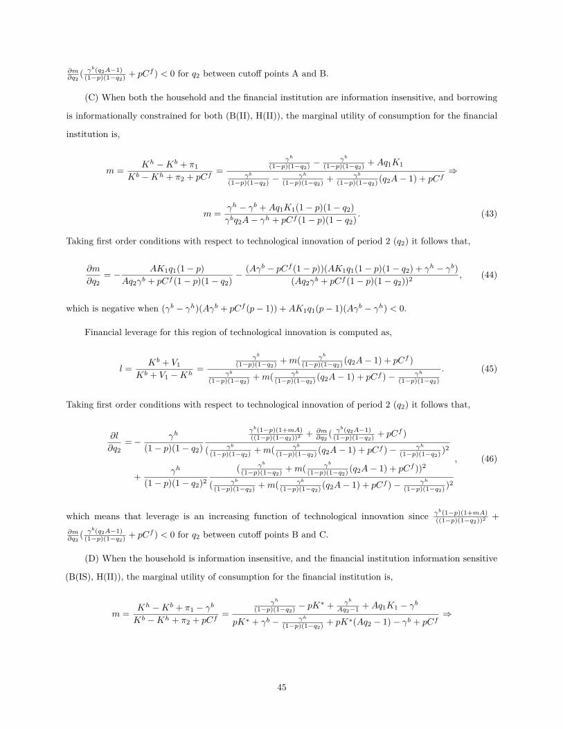
∂m∂q2

( γb(q2A−1)(1−p)(1−q2) + pCf ) < 0 for q2 between cutoff points A and B.

(C) When both the household and the financial institution are information insensitive, and borrowing

is informationally constrained for both (B(II), H(II)), the marginal utility of consumption for the financial

institution is,

m = Kh −Kb + π1

Kb −Kh + π2 + pCf=

γh

(1−p)(1−q2) −γb

(1−p)(1−q2) +Aq1K1γb

(1−p)(1−q2) −γh

(1−p)(1−q2) + γb

(1−p)(1−q2) (q2A− 1) + pCf⇒

m = γh − γb +Aq1K1(1− p)(1− q2)γbq2A− γh + pCf (1− p)(1− q2) . (43)

Taking first order conditions with respect to technological innovation of period 2 (q2) it follows that,

∂m

∂q2= − AK1q1(1− p)

Aq2γb + pCf (1− p)(1− q2) −(Aγb − pCf (1− p))(AK1q1(1− p)(1− q2) + γh − γb)

(Aq2γb + pCf (1− p)(1− q2))2 , (44)

which is negative when (γb − γh)(Aγb + pCf (p− 1)) +AK1q1(p− 1)(Aγb − γh) < 0.

Financial leverage for this region of technological innovation is computed as,

l = Kb + V1

Kb + V1 −Kh=

γb

(1−p)(1−q2) +m( γb

(1−p)(1−q2) (q2A− 1) + pCf )γb

(1−p)(1−q2) +m( γb

(1−p)(1−q2) (q2A− 1) + pCf )− γh

(1−p)(1−q2)

. (45)

Taking first order conditions with respect to technological innovation of period 2 (q2) it follows that,

∂l

∂q2=− γh

(1− p)(1− q2)

γb(1−p)(1+mA)((1−p)(1−q2))2 + ∂m

∂q2( γb(q2A−1)

(1−p)(1−q2) + pCf )

( γb

(1−p)(1−q2) +m( γb

(1−p)(1−q2) (q2A− 1) + pCf )− γh

(1−p)(1−q2) )2

+ γh

(1− p)(1− q2)2

( γb

(1−p)(1−q2) +m( γb

(1−p)(1−q2) (q2A− 1) + pCf ))2

( γb

(1−p)(1−q2) +m( γb

(1−p)(1−q2) (q2A− 1) + pCf )− γh

(1−p)(1−q2) )2

, (46)

which means that leverage is an increasing function of technological innovation since γb(1−p)(1+mA)((1−p)(1−q2))2 +

∂m∂q2

( γb(q2A−1)(1−p)(1−q2) + pCf ) < 0 for q2 between cutoff points B and C.

(D) When the household is information insensitive, and the financial institution information sensitive

(B(IS), H(II)), the marginal utility of consumption for the financial institution is,

m = Kh −Kb + π1 − γb

Kb −Kh + π2 + pCf=

γh

(1−p)(1−q2) − pK∗ + γb

Aq2−1 +Aq1K1 − γb

pK∗ + γb − γh

(1−p)(1−q2) + pK∗(Aq2 − 1)− γb + pCf⇒

45

m =γh

(1−p)(1−q2) − pK∗ + γb

Aq2−1 +Aq1K1 − γb

pK∗Aq2 − γh

(1−p)(1−q2) + pCf. (47)

Taking first order conditions with respect to technological innovation of period 2 (q2) it follows that,

∂m

∂q2=

( γh

(1−p)(1−q2)2 − γbA(Aq2−1)2 )(pK∗Aq2 − γh

(1−p)(1−q2) + pCf )

(pK∗Aq2 − γh

(1−p)(1−q2) + pCf )2

−( γh

(1−p)(1−q2) − pK∗ + γb

Aq2−1 − γb)(pK∗A− γh

(1−p)(1−q2)2 )

(pK∗Aq2 − γh

(1−p)(1−q2) + pCf )2

(48)

which is positive since Aq1K1( γh

(1−p)(1−q2)2 −pK∗A) + γhAAq2−1 ( γh

1−q2−pK∗Aq2−pCf ) ≥ 0 for q2 between cutoff

points C and D.

Financial leverage for this region of technological innovation is computed as,

l = Kb + V1

Kb + V1 −Kh=

pK∗ − γb

Aq2−1 +m(pK∗(q2A− 1)− γb + pCf )

pK∗ − γb

Aq2−1 +m(pK∗(q2A− 1)− γb + pCf )− γh

(1−p)(1−q2)

. (49)

Taking first order conditions with respect to technological innovation of period 2 (q2) it follows that,

∂l

∂q2=− γh

(1− p)(1− q2)

γbA(Aq2−1)2 + ∂m

∂q2(pK∗(q2A− 1)− γb + pCf ) +mpK∗A

(pK∗ − γb

Aq2−1 +m(pK∗(q2A− 1)− γb + pCf )− γh

(1−p)(1−q2) )2

+ γh

(1− p)(1− q2)2

(pK∗ − γb

Aq2−1 +m(pK∗(q2A− 1)− γb + pCf )

(pK∗ − γb

Aq2−1 +m(pK∗(q2A− 1)− γb + pCf )− γh

(1−p)(1−q2) )2,

, (50)

which means that leverage is an increasing function of technological innovation since γbA(Aq2−1)2 + ∂m

∂q2(pK∗(q2A−

1)− γb + pCf ) +mpK∗A < 0 for q2 between cutoff points C and D.

(E): The proof follows the same logic.

46

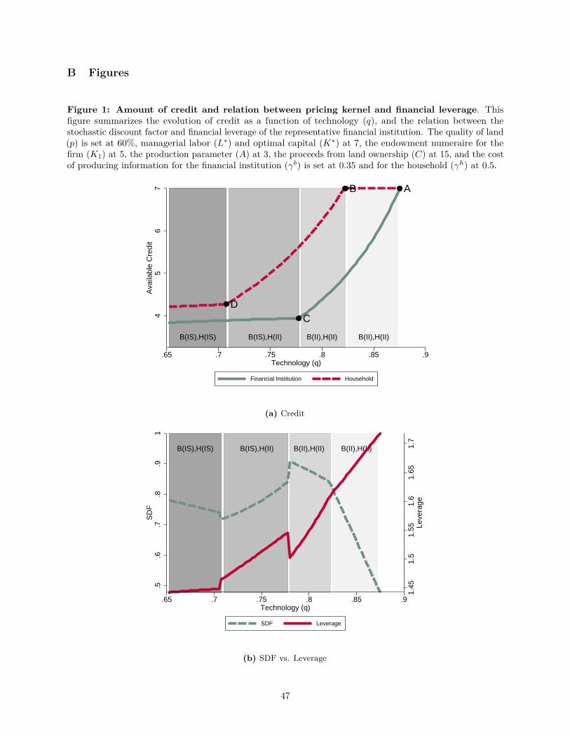
B Figures

Figure 1: Amount of credit and relation between pricing kernel and financial leverage. Thisfigure summarizes the evolution of credit as a function of technology (q), and the relation between thestochastic discount factor and financial leverage of the representative financial institution. The quality of land(p) is set at 60%, managerial labor (L∗) and optimal capital (K∗) at 7, the endowment numeraire for thefirm (K1) at 5, the production parameter (A) at 3, the proceeds from land ownership (C) at 15, and the costof producing information for the financial institution (γb) is set at 0.35 and for the household (γh) at 0.5.

DC

B A

B(II),H(II)B(II),H(II)B(IS),H(II)B(IS),H(IS)

45

67

Ava

ilabl

e C

redi

t

.65 .7 .75 .8 .85 .9Technology (q)

Financial Institution Household

(a) Credit

B(II),H(II)B(II),H(II)B(IS),H(II)B(IS),H(IS)

1.45

1.5

1.55

1.6

1.65

1.7

Leve

rage

.5.6

.7.8

.91

SD

F

.65 .7 .75 .8 .85 .9Technology (q)

SDF Leverage

(b) SDF vs. Leverage

47

Figure 2: Financial Leverage and Financial Intermediaries’ Future Assets Across CreditRegimes (Individual Country Series). The figure summarizes the relation between future asset levels offinancial intermediaries and global financial leverage across different credit regimes: (i) a high credit regimedefined as instances where credit-to-private sector of a given country is higher than the 75th percentile ofits historical credit series, and (ii) a low credit regime defined as instances where credit-to-private sectorof a given country is lower than the 25th percentile of its historical credit series. The regression specifi-cation is: assetst+1 = α + β′Xt + γassetst + εt+1, where Xt = (fin.leverage, fin.leverage × 1(Creditt >75%), fin.leverage × 1(Creditt < 25%))′. Lowercase variables are log variables. Data are quarterly fromDataStream, WorldScope, and the World Development Indicators database, and span a period from 2001until 2014. Standard errors are heteroskedasticity- (White (1980)) and autocorrelation-robust (Newey andWest (1987) and Newey and West (1994)).

−1

−.5

0.5

Coe

ffici

ent

Aus

tria

Bel

gium

Bra

zil

Bul

garia

Can

ada

Chi

leC

olom

bia

Cro

atia

Cyp

rus

Che

ch R

epub

licD

enm

ark

Fin

land

Fra

nce

Ger

man

yG

reec

eH

ong

Kon

gH

unga

ryIc

elan

dIn

done

sia

Isra

elIta

lyJa

pan

Kaz

akhs

tan

Ken

yaS

outh

Kor

eaK

uwai

tM

alay

sia

Mex

ico

Net

herla

nds

New

Zea

land

Nor

way

Om

anP

akis

tan

Per

uP

hilip

pine

sP

olan

dP

ortu

gal

Qat

arR

oman

iaR

ussi

aS

audi

Ara

bia

Sin

gapo

reS

lova

kia

Slo

veni

aS

pain

Sw

eden

Sw

itzer

land

Tha

iland

Ukr

aine

UA

EU

nite

d K

ingd

omU

nite

d S

tate

sV

enez

uela

Country

(a) fin.leverage× 1(Creditt < 25%)

−.2

0.2

.4.6

.8C

oeffi

cien

t

Aus

tria

Bel

gium

Bra

zil

Bul

garia

Can

ada

Chi

leC

olom

bia

Cro

atia

Cyp

rus

Che

ch R

epub

licD

enm

ark

Fin

land

Fra

nce

Ger

man

yG

reec

eH

ong

Kon

gH

unga

ryIc

elan

dIn

done

sia

Isra

elIta

lyJa

pan

Kaz

akhs

tan

Ken

yaS

outh

Kor

eaK

uwai

tM

alay

sia

Mex

ico

Net

herla

nds

New

Zea

land

Nor

way

Om

anP

akis

tan

Per

uP

hilip

pine

sP

olan

dP

ortu

gal

Qat

arR

oman

iaR

ussi

aS

audi

Ara

bia

Sin

gapo

reS

lova

kia

Slo

veni

aS

pain

Sw

eden

Sw

itzer

land

Tha

iland

Ukr

aine

UA

EU

nite

d K

ingd

omU

nite

d S

tate

sV

enez

uela

Country

(b) fin.leverage× 1(Creditt > 75%)

−20

−10

010

Coe

ffici

ent

Aus

tria

Bel

gium

Bra

zil

Bul

garia

Can

ada

Chi

leC

olom

bia

Cro

atia

Cyp

rus

Che

ch R

epub

licD

enm

ark

Fin

land

Fra

nce

Ger

man

yG

reec

eH

ong

Kon

gH

unga

ryIc

elan

dIn

done

sia

Isra

elIta

lyJa

pan

Kaz

akhs

tan

Ken

yaS

outh

Kor

eaK

uwai

tM

alay

sia

Mex

ico

Net

herla

nds

New

Zea

land

Nor

way

Om

anP

akis

tan

Per

uP

hilip

pine

sP

olan

dP

ortu

gal

Qat

arR

oman

iaR

ussi

aS

audi

Ara

bia

Sin

gapo

reS

lova

kia

Slo

veni

aS

pain

Sw

eden

Sw

itzer

land

Tha

iland

Ukr

aine

UA

EU

nite

d K

ingd

omU

nite

d S

tate

sV

enez

uela

Country

(c) fin.leverage

−1

−.5

0.5

11.

5C

oeffi

cien

t

Aus

tria

Bel

gium

Bra

zil

Bul

garia

Can

ada

Chi

leC

olom

bia

Cro

atia

Cyp

rus

Che

ch R

epub

licD

enm

ark

Fin

land

Fra

nce

Ger

man

yG

reec

eH

ong

Kon

gH

unga

ryIc

elan

dIn

done

sia

Isra

elIta

lyJa

pan

Kaz

akhs

tan

Ken

yaS

outh

Kor

eaK

uwai

tM

alay

sia

Mex

ico

Net

herla

nds

New

Zea

land

Nor

way

Om

anP

akis

tan

Per

uP

hilip

pine

sP

olan

dP

ortu

gal

Qat

arR

oman

iaR

ussi

aS

audi

Ara

bia

Sin

gapo

reS

lova

kia

Slo

veni

aS

pain

Sw

eden

Sw

itzer

land

Tha

iland

Ukr

aine

UA

EU

nite

d K

ingd

omU

nite

d S

tate

sV

enez

uela

Country

(d) financial assets

48

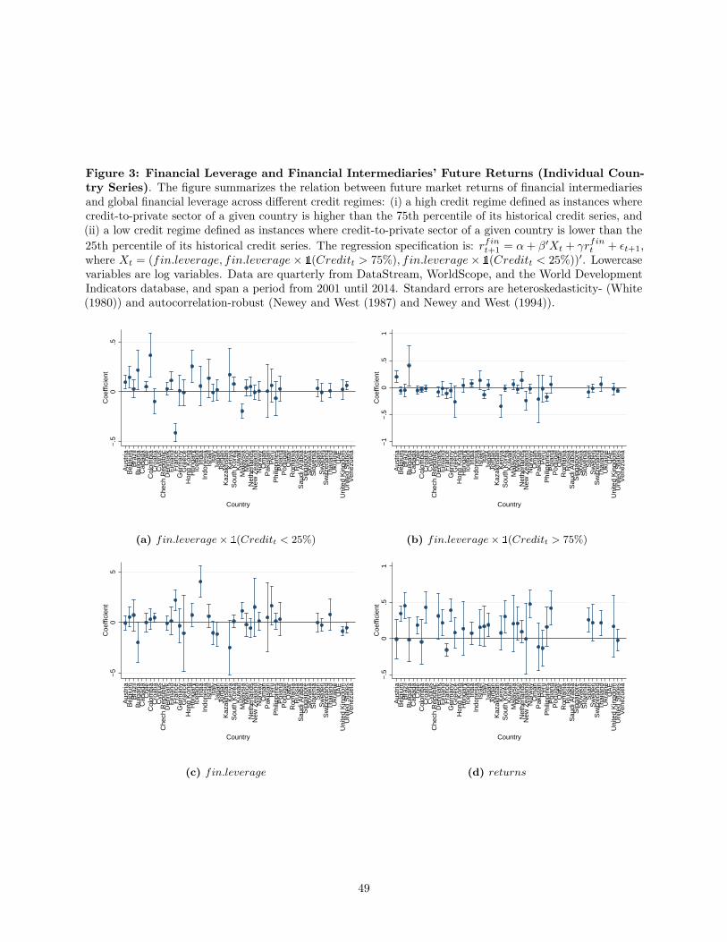
Figure 3: Financial Leverage and Financial Intermediaries’ Future Returns (Individual Coun-try Series). The figure summarizes the relation between future market returns of financial intermediariesand global financial leverage across different credit regimes: (i) a high credit regime defined as instances wherecredit-to-private sector of a given country is higher than the 75th percentile of its historical credit series, and(ii) a low credit regime defined as instances where credit-to-private sector of a given country is lower than the25th percentile of its historical credit series. The regression specification is: rfint+1 = α+ β′Xt + γrfint + εt+1,where Xt = (fin.leverage, fin.leverage× 1(Creditt > 75%), fin.leverage× 1(Creditt < 25%))′. Lowercasevariables are log variables. Data are quarterly from DataStream, WorldScope, and the World DevelopmentIndicators database, and span a period from 2001 until 2014. Standard errors are heteroskedasticity- (White(1980)) and autocorrelation-robust (Newey and West (1987) and Newey and West (1994)).

−.5

0.5

Coe

ffici

ent

Aus

tria

Bel

gium

Bra

zil

Bul

garia

Can

ada

Chi

leC

olom

bia

Cro

atia

Cyp

rus

Che

ch R

epub

licD

enm

ark

Fin

land

Fra

nce

Ger

man

yG

reec

eH

ong

Kon

gH

unga

ryIc

elan

dIn

dia

Indo

nesi

aIs

rael

Italy

Japa

nJo

rdan

Kaz

akhs

tan

Ken

yaS

outh

Kor

eaK

uwai

tM

alay

sia

Mex

ico

Net

herla

nds

New

Zea

land

Nor

way

Om

anP

akis

tan

Per

uP

hilip

pine

sP

olan

dP

ortu

gal

Qat

arR

oman

iaR

ussi

aS

audi

Ara

bia

Sin

gapo

reS

lova

kia

Slo

veni

aS

pain

Sw

eden

Sw

itzer

land

Tha

iland

Ukr

aine

UA

EU

nite

d K

ingd

omU

nite

d S

tate

sV

enez

uela

Country

(a) fin.leverage× 1(Creditt < 25%)

−1

−.5

0.5

1C

oeffi

cien

t

Aus

tria

Bel

gium

Bra

zil

Bul

garia

Can

ada

Chi

leC

olom

bia

Cro

atia

Cyp

rus

Che

ch R

epub

licD

enm

ark

Fin

land

Fra

nce

Ger

man

yG

reec

eH

ong

Kon

gH

unga

ryIc

elan

dIn

dia

Indo

nesi

aIs

rael

Italy

Japa

nJo

rdan

Kaz

akhs

tan

Ken

yaS

outh

Kor

eaK

uwai

tM

alay

sia

Mex

ico

Net

herla

nds

New

Zea

land

Nor

way

Om

anP

akis

tan

Per

uP

hilip

pine

sP

olan

dP

ortu

gal

Qat

arR

oman

iaR

ussi

aS

audi

Ara

bia

Sin

gapo

reS

lova

kia

Slo

veni

aS

pain

Sw

eden

Sw

itzer

land

Tha

iland

Ukr

aine

UA

EU

nite

d K

ingd

omU

nite

d S

tate

sV

enez

uela

Country

(b) fin.leverage× 1(Creditt > 75%)

−5

05

Coe

ffici

ent

Aus

tria

Bel

gium

Bra

zil

Bul

garia

Can

ada

Chi

leC

olom

bia

Cro

atia

Cyp

rus

Che

ch R

epub

licD

enm

ark

Fin

land

Fra

nce

Ger

man

yG

reec

eH

ong

Kon

gH

unga

ryIc

elan

dIn

dia

Indo

nesi

aIs

rael

Italy

Japa

nJo

rdan

Kaz

akhs

tan

Ken

yaS

outh

Kor

eaK

uwai

tM

alay

sia

Mex

ico

Net

herla

nds

New

Zea

land

Nor

way

Om

anP

akis

tan

Per

uP

hilip

pine

sP

olan

dP

ortu

gal

Qat

arR

oman

iaR

ussi

aS

audi

Ara

bia

Sin

gapo

reS

lova

kia

Slo

veni

aS

pain

Sw

eden

Sw

itzer

land

Tha

iland

Ukr

aine

UA

EU

nite

d K

ingd

omU

nite

d S

tate

sV

enez

uela

Country

(c) fin.leverage

−.5

0.5

1C

oeffi

cien

t

Aus

tria

Bel

gium

Bra

zil

Bul

garia

Can

ada

Chi

leC

olom

bia

Cro

atia

Cyp

rus

Che

ch R

epub

licD

enm

ark

Fin

land

Fra

nce

Ger

man

yG

reec

eH

ong

Kon

gH

unga

ryIc

elan

dIn

dia

Indo

nesi

aIs

rael

Italy

Japa

nJo

rdan

Kaz

akhs

tan

Ken

yaS

outh

Kor

eaK

uwai

tM

alay

sia

Mex

ico

Net

herla

nds

New

Zea

land

Nor

way

Om

anP

akis

tan

Per

uP

hilip

pine

sP

olan

dP

ortu

gal

Qat

arR

oman

iaR

ussi

aS

audi

Ara

bia

Sin

gapo

reS

lova

kia

Slo

veni

aS

pain

Sw

eden

Sw

itzer

land

Tha

iland

Ukr

aine

UA

EU

nite

d K

ingd

omU

nite

d S

tate

sV

enez

uela

Country

(d) returns

49

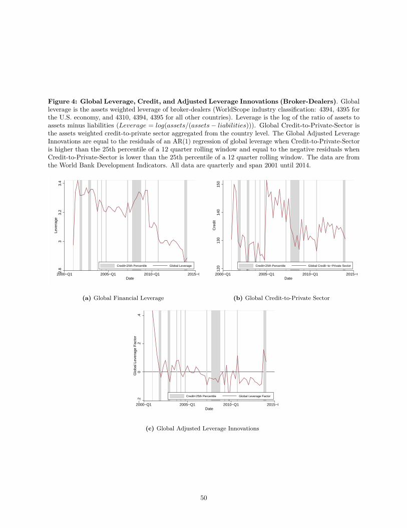
Figure 4: Global Leverage, Credit, and Adjusted Leverage Innovations (Broker-Dealers). Globalleverage is the assets weighted leverage of broker-dealers (WorldScope industry classification: 4394, 4395 forthe U.S. economy, and 4310, 4394, 4395 for all other countries). Leverage is the log of the ratio of assets toassets minus liabilities (Leverage = log(assets/(assets − liabilities))). Global Credit-to-Private-Sector isthe assets weighted credit-to-private sector aggregated from the country level. The Global Adjusted LeverageInnovations are equal to the residuals of an AR(1) regression of global leverage when Credit-to-Private-Sectoris higher than the 25th percentile of a 12 quarter rolling window and equal to the negative residuals whenCredit-to-Private-Sector is lower than the 25th percentile of a 12 quarter rolling window. The data are fromthe World Bank Development Indicators. All data are quarterly and span 2001 until 2014.

2.8

33.

23.

4Le

vera

ge

2000−Q1 2005−Q1 2010−Q1 2015−Q1Date

Credit<25th Percentile Global Leverage

(a) Global Financial Leverage

120

130

140

150

Cre

dit

2000−Q1 2005−Q1 2010−Q1 2015−Q1Date

Credit<25th Percentile Global Credit−to−Private Sector

(b) Global Credit-to-Private Sector

−.2

0.2

.4G

loba

l Lev

erag

e F

acto

r

2000−Q1 2005−Q1 2010−Q1 2015−Q1Date

Credit<25th Percentile Global Leverage Factor

(c) Global Adjusted Leverage Innovations

50

Figure 5: Global Leverage Innovations vs. Adjusted Leverage Innovations (Broker-Dealers).Global leverage Innovations are the residuals of an AR(1) regression of global leverage. Global AdjustedLeverage Innovations are equal to the residuals of an AR(1) regression of global leverage when Credit-to-Private-Sector is higher than the 25th percentile of a 12 quarter rolling window and equal to the negativeresiduals when Credit-to-Private-Sector is lower than the 25th percentile of a 12 quarter rolling window. Thedata are from WorldScope (industry classification: 4394, 4395 for the U.S. economy, and 4310, 4394, 4395 forall other countries) and the World Bank Development Indicators. All data are quarterly and span 2001 until2014.

−.4

−.2

0.2

.4Le

vera

ge F

acto

r

2000−Q1 2005−Q1 2010−Q1 2015−Q1Date

Credit<25th Percentile Global Leverage Factor

Leverage Innovations

51

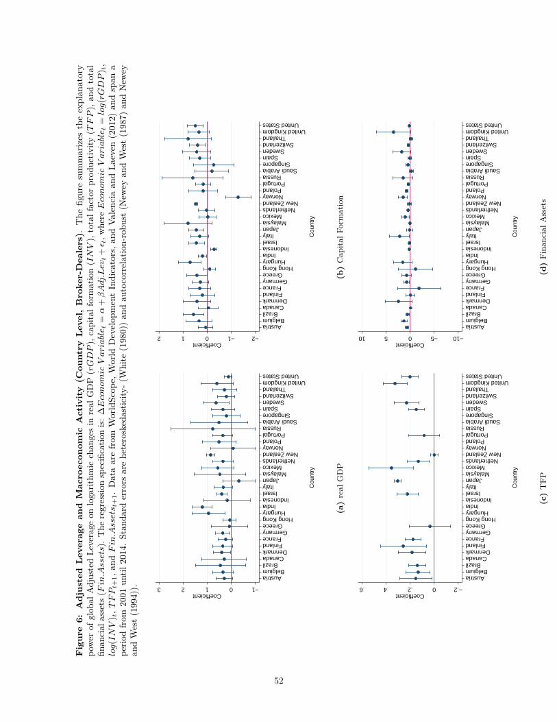
Figure6:

AdjustedLe

verage

andMacroecon

omic

Activity(C

ountry

Level,Broker-Dealers).

The

figuresummarizes

theexplan

atory

powe

rof

glob

alAdjustedLe

verage

onloga

rithm

icchan

gesin

real

GDP

(rGDP),

capitalformation(INV),

totalfactorprod

uctiv

ity(TFP),

andtotal

finan

cial

assets

(Fin.Assets).The

regressio

nspecificatio

nis:

∆Econom

icVariable t

=α

+βAdj.Levt+ε t,w

hereEconom

icVariable t

=log(rGDP

) t,

log(INV

) t,T

FPt+

1,an

dFin.Assets t

+1.

Dataarefrom

WorldSc

ope,

World

Develop

mentIndicators,a

ndVa

lenc

iaan

dLa

even

(2012)

andspan

ape

riodfrom

2001

until

2014.Stan

dard

errors

arehe

terosked

astic

ity-(

White

(1980))an

dau

tocorrelation-robu

st(N

ewey

andWest(1987)

andNew

eyan

dWest(1994)). −10123

Coefficient

AustriaBelgium

BrazilCanada

DenmarkFinlandFrance

GermanyGreece

Hong KongHungary

IndiaIndonesia

IsraelItaly

JapanMalaysia

MexicoNetherlands

New ZealandNorwayPoland

PortugalRussia

Saudi ArabiaSingapore

SpainSweden

SwitzerlandThailand

United KingdomUnited States

Cou

ntry

(a)real

GDP

−2−1012Coefficient

AustriaBelgium

BrazilCanada

DenmarkFinlandFrance

GermanyGreece

Hong KongHungary

IndiaIndonesia

IsraelItaly

JapanMalaysia

MexicoNetherlands

New ZealandNorwayPoland

PortugalRussia

Saudi ArabiaSingapore

SpainSweden

SwitzerlandThailand

United KingdomUnited States

Cou

ntry

(b)Cap

italF

ormation

−.20.2.4.6Coefficient

AustriaBelgium

BrazilCanada

DenmarkFinlandFrance

GermanyGreece

Hong KongHungary

IndiaIndonesia

IsraelItaly

JapanMalaysia

MexicoNetherlands

New ZealandNorwayPoland

PortugalRussia

Saudi ArabiaSingapore

SpainSweden

SwitzerlandThailand

United KingdomUnited States

Cou

ntry

(c)TFP

−10−50510Coefficient

AustriaBelgium

BrazilCanada

DenmarkFinlandFrance

GermanyGreece

Hong KongHungary

IndiaIndonesia

IsraelItaly

JapanMalaysia

MexicoNetherlands

New ZealandNorwayPoland

PortugalRussia

Saudi ArabiaSingapore

SpainSweden

SwitzerlandThailand

United KingdomUnited States

Cou

ntry

(d)Fina

ncialA

ssets

52

Figure7:

AdjustedLe

verage

andMacroecon

omic

Activity(C

ountry

Level,Broker-Dealers).

The

figuresummarizes

theexplan

atory

power

ofglob

alAdjustedLe

verage

onlogarit

hmic

chan

gesin

househ

oldcred

it(H

H.Cr),c

orpo

rate

cred

it(Corp.Cr),a

ndtotalg

loba

limba

lanc

es(GI(Total)).

The

regressio

nspecificatio

nis:

∆Econom

icVariable t

=α

+βAdj.Levt+ε t,w

hereEconom

icVariable t

=(log

(HH.Cr)t,log

(Corp.Cr)t,

andlog(GI(Total)

) t).

Dataarefrom

WorldSc

opean

dWorld

Develop

mentIndicators,a

ndspan

ape

riodfrom

2001

until

2014

.Stan

dard

errors

are

heterosked

astic

ity-(

White

(1980))an

dau

tocorrelation-robu

st(N

ewey

andWest(1987)

andNew

eyan

dWest(1994)).

−.2−.10.1.2.3Coefficient

AustriaBelgium

BrazilCanada

DenmarkFinlandFrance

GermanyGreece

Hong KongHungary

IndiaIndonesia

IsraelItaly

JapanMalaysia

MexicoNetherlands

New ZealandNorwayPoland

PortugalRussia

Saudi ArabiaSingapore

SpainSweden

SwitzerlandThailand

United KingdomUnited States

Cou

ntry

(a)Hou

seho

ldCredit

−.4−.20.2.4Coefficient

AustriaBelgium

BrazilCanada

DenmarkFinlandFrance

GermanyGreece

Hong KongHungary

IndiaIndonesia

IsraelItaly

JapanMalaysia

MexicoNetherlands

New ZealandNorwayPoland

PortugalRussia

Saudi ArabiaSingapore

SpainSweden

SwitzerlandThailand

United KingdomUnited States

Cou

ntry

(b)Corpo

rate

Credit

−60−40−20020Coefficient

AustriaBelgium

BrazilCanada

DenmarkFinlandFrance

GermanyGreece

Hong KongHungary

IndiaIndonesia

IsraelItaly

JapanMalaysia

MexicoNetherlands

New ZealandNorwayPoland

PortugalRussia

Saudi ArabiaSingapore

SpainSweden

SwitzerlandThailand

United KingdomUnited States

Cou

ntry

(c)Globa

lImba

lances

(Total)

53

Figure 8: Adjusted Leverage, Future Consumption (Non-Durables, Durables), and Future Pri-vate Investments (U.S. Economy). This figure summarizes the predictive power of global AdjustedLeverage on (a) future logarithmic changes of non-durables consumption (log(Cndt+q/Cndt )), (b) future logarith-mic changes of durables consumption (log(Cdt+q/Cdt )), and (c) future private investment (log(INVt+q/INVt))for the U.S. economy. The regression specification is: log(Xt+q/Xt) = αt+q + βAdj.Levt + εt+q whereXt = (Cndt , Cdt , INVt). The data are quarterly and span a period from 2001-Q1 until 2014-Q1. Standarderrors are heteroskedasticity- (White (1980)) and autocorrelation-robust (Newey and West (1987) and Neweyand West (1994)).

−.1

0.1

.2.3

Coe

ffici

ent

1 2 3 4 5 6 7 8 9 10 11 12 13 14 15 16 17 18 19 20

Quarters from time t (k)

(a) Non-Durables (Coefficient)

0.0

5.1

.15

R−

Squ

ared

1 2 3 4 5 6 7 8 9 10 11 12 13 14 15 16 17 18 19 20

Quarters from time t (k)

(b) Non-Durables (R-Squared)

−.2

0.2

.4.6

Coe

ffici

ent

1 2 3 4 5 6 7 8 9 10 11 12 13 14 15 16 17 18 19 20

Quarters from time t (k)

(c) Durables (Coefficient)

0.0

2.0

4.0

6.0

8R

−S

quar

ed

1 2 3 4 5 6 7 8 9 10 11 12 13 14 15 16 17 18 19 20

Quarters from time t (k)

(d) Durables (R-Squared)

−.2

0.2

.4.6

.8C

oeffi

cien

t

1 2 3 4 5 6 7 8 9 10 11 12 13 14 15 16 17 18 19 20

Quarters from time t (k)

(e) Investments (Coefficient)

0.0

5.1

.15

R−

Squ

ared

1 2 3 4 5 6 7 8 9 10 11 12 13 14 15 16 17 18 19 20

Quarters from time t (k)

(f) Investments (R-Squared)54

Figure 9: Realized vs. Predicted Mean Returns. This figure summarizes the realized averageannualized returns of 25 value-weighted Fama-French global equity portfolios sorted on size and book-to-marketagainst the average returns predicted by four linear pricing models (Adjusted Leverage, Global Market,Global Fama-French Factors, and Global Fama-French Factors & Momentum) with an intercept. Thedata are quarterly and span a period from 2001-Q1 until 2014-Q1. All returns are annualized.

−0.04 −0.02 0 0.02 0.04 0.06 0.08 0.1 0.12 0.14 0.16 0.18 0.2 0.22 0.24−0.04

−0.02

0

0.02

0.04

0.06

0.08

0.1

0.12

0.14

0.16

0.18

0.2

0.22

0.24

S1B1

S1B2

S1B3S1B4

S1B5

S2B1

S2B2 S2B3

S2B4

S2B5

S3B1

S3B2

S3B3S3B4

S3B5

S4B1

S4B2S4B3 S4B4S4B5

S5B1

S5B2S5B3S5B4

S5B5

Predicted Expected Return

Rea

lized

Mea

n R

etur

n

(a) Adjusted Leverage

−0.04 −0.02 0 0.02 0.04 0.06 0.08 0.1 0.12 0.14 0.16 0.18 0.2 0.22 0.24−0.04

−0.02

0

0.02

0.04

0.06

0.08

0.1

0.12

0.14

0.16

0.18

0.2

0.22

0.24

S1B1

S1B2

S1B3S1B4

S1B5

S2B1

S2B2 S2B3

S2B4

S2B5

S3B1

S3B2

S3B3S3B4

S3B5

S4B1

S4B2S4B3 S4B4S4B5

S5B1

S5B2S5B3S5B4

S5B5

Predicted Expected Return

Rea

lized

Mea

n R

etur

n

(b) Global Market

−0.04 −0.02 0 0.02 0.04 0.06 0.08 0.1 0.12 0.14 0.16 0.18 0.2 0.22 0.24−0.04

−0.02

0

0.02

0.04

0.06

0.08

0.1

0.12

0.14

0.16

0.18

0.2

0.22

0.24

S1B1

S1B2

S1B3S1B4

S1B5

S2B1

S2B2 S2B3

S2B4

S2B5

S3B1

S3B2

S3B3S3B4

S3B5

S4B1

S4B2S4B3 S4B4S4B5

S5B1

S5B2S5B3S5B4

S5B5

Predicted Expected Return

Rea

lized

Mea

n R

etur

n

(c) Global Fama-French Factors

−0.04 −0.02 0 0.02 0.04 0.06 0.08 0.1 0.12 0.14 0.16 0.18 0.2 0.22 0.24−0.04

−0.02

0

0.02

0.04

0.06

0.08

0.1

0.12

0.14

0.16

0.18

0.2

0.22

0.24

S1B1

S1B2

S1B3S1B4

S1B5

S2B1

S2B2 S2B3

S2B4

S2B5

S3B1

S3B2

S3B3S3B4

S3B5

S4B1

S4B2S4B3S4B4S4B5

S5B1

S5B2S5B3S5B4

S5B5

Predicted Expected Return

Rea

lized

Mea

n R

etur

n

(d) Global Fama-French Factors & Momentum

55

Figure 10: Realized vs. Predicted Mean Returns. This figure summarizes the realized averageannualized returns of 25 value-weighted Fama-French global equity portfolios sorted on size and momentumagainst the average returns predicted by four linear pricing models (Adjusted Leverage, Global Market,Global Fama-French Factors, and Global Fama-French Factors & Momentum) with an intercept. Thedata are quarterly and span a period from 2001-Q1 until 2014-Q1. All returns are annualized.

−0.04 −0.02 0 0.02 0.04 0.06 0.08 0.1 0.12 0.14 0.16 0.18 0.2 0.22 0.24−0.04

−0.02

0

0.02

0.04

0.06

0.08

0.1

0.12

0.14

0.16

0.18

0.2

0.22

0.24

S1M1

S1M2

S1M3

S1M4

S1M5

S2M1

S2M2S2M3

S2M4

S2M5

S3M1S3M2

S3M3S3M4

S3M5

S4M1

S4M2

S4M3S4M4

S4M5

S5M1

S5M2S5M3

S5M4S5M5

Predicted Expected Return

Rea

lized

Mea

n R

etur

n

(a) Adjusted Leverage

−0.04 −0.02 0 0.02 0.04 0.06 0.08 0.1 0.12 0.14 0.16 0.18 0.2 0.22 0.24−0.04

−0.02

0

0.02

0.04

0.06

0.08

0.1

0.12

0.14

0.16

0.18

0.2

0.22

0.24

S1M1

S1M2

S1M3

S1M4

S1M5

S2M1

S2M2S2M3

S2M4

S2M5

S3M1S3M2

S3M3S3M4

S3M5

S4M1

S4M2

S4M3S4M4

S4M5

S5M1

S5M2S5M3

S5M4S5M5

Predicted Expected Return

Rea

lized

Mea

n R

etur

n

(b) Global Market

−0.04 −0.02 0 0.02 0.04 0.06 0.08 0.1 0.12 0.14 0.16 0.18 0.2 0.22 0.24−0.04

−0.02

0

0.02

0.04

0.06

0.08

0.1

0.12

0.14

0.16

0.18

0.2

0.22

0.24

S1M1

S1M2

S1M3

S1M4

S1M5

S2M1

S2M2S2M3

S2M4

S2M5

S3M1S3M2

S3M3S3M4

S3M5

S4M1

S4M2

S4M3S4M4

S4M5

S5M1

S5M2S5M3

S5M4S5M5

Predicted Expected Return

Rea

lized

Mea

n R

etur

n

(c) Global Fama-French Factors

−0.04 −0.02 0 0.02 0.04 0.06 0.08 0.1 0.12 0.14 0.16 0.18 0.2 0.22 0.24−0.04

−0.02

0

0.02

0.04

0.06

0.08

0.1

0.12

0.14

0.16

0.18

0.2

0.22

0.24

S1M1

S1M2

S1M3

S1M4

S1M5

S2M1

S2M2S2M3

S2M4

S2M5

S3M1S3M2

S3M3S3M4

S3M5

S4M1

S4M2

S4M3S4M4

S4M5

S5M1

S5M2S5M3

S5M4S5M5

Predicted Expected Return

Rea

lized

Mea

n R

etur

n

(d) Global Fama-French Factors & Momentum

56

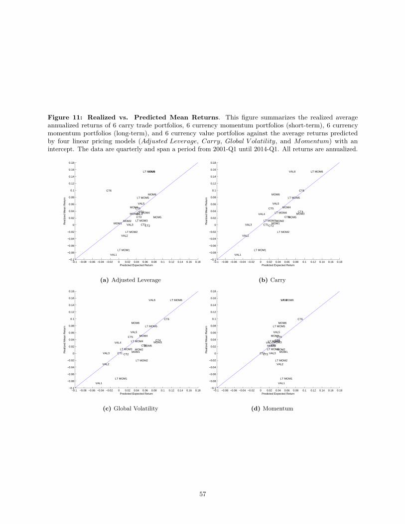
Figure 11: Realized vs. Predicted Mean Returns. This figure summarizes the realized averageannualized returns of 6 carry trade portfolios, 6 currency momentum portfolios (short-term), 6 currencymomentum portfolios (long-term), and 6 currency value portfolios against the average returns predictedby four linear pricing models (Adjusted Leverage, Carry, Global V olatility, and Momentum) with anintercept. The data are quarterly and span a period from 2001-Q1 until 2014-Q1. All returns are annualized.

−0.1 −0.08 −0.06 −0.04 −0.02 0 0.02 0.04 0.06 0.08 0.1 0.12 0.14 0.16 0.18−0.1

−0.08

−0.06

−0.04

−0.02

0

0.02

0.04

0.06

0.08

0.1

0.12

0.14

0.16

0.18

CT1CT2

CT3

CT4CT5

CT6

MOM1MOM2

MOM3

MOM4

MOM5

MOM6

LT MOM1

LT MOM2

LT MOM3

LT MOM4

LT MOM5

LT MOM6

VAL1

VAL2

VAL3

VAL4

VAL5

VAL6

Predicted Expected Return

Rea

lized

Mea

n R

etur

n

(a) Adjusted Leverage

−0.1 −0.08 −0.06 −0.04 −0.02 0 0.02 0.04 0.06 0.08 0.1 0.12 0.14 0.16 0.18−0.1

−0.08

−0.06

−0.04

−0.02

0

0.02

0.04

0.06

0.08

0.1

0.12

0.14

0.16

0.18

CT1CT2

CT3

CT4CT5

CT6

MOM1MOM2

MOM3

MOM4

MOM5

MOM6

LT MOM1

LT MOM2

LT MOM3

LT MOM4

LT MOM5

LT MOM6

VAL1

VAL2

VAL3

VAL4

VAL5

VAL6

Predicted Expected Return

Rea

lized

Mea

n R

etur

n

(b) Carry

−0.1 −0.08 −0.06 −0.04 −0.02 0 0.02 0.04 0.06 0.08 0.1 0.12 0.14 0.16 0.18−0.1

−0.08

−0.06

−0.04

−0.02

0

0.02

0.04

0.06

0.08

0.1

0.12

0.14

0.16

0.18

CT1 CT2

CT3

CT4CT5

CT6

MOM1MOM2

MOM3

MOM4

MOM5

MOM6

LT MOM1

LT MOM2

LT MOM3

LT MOM4

LT MOM5

LT MOM6

VAL1

VAL2

VAL3

VAL4

VAL5

VAL6

Predicted Expected Return

Rea

lized

Mea

n R

etur

n

(c) Global Volatility

−0.1 −0.08 −0.06 −0.04 −0.02 0 0.02 0.04 0.06 0.08 0.1 0.12 0.14 0.16 0.18−0.1

−0.08

−0.06

−0.04

−0.02

0

0.02

0.04

0.06

0.08

0.1

0.12

0.14

0.16

0.18

CT1CT2

CT3

CT4CT5

CT6

MOM1MOM2

MOM3

MOM4

MOM5

MOM6

LT MOM1

LT MOM2

LT MOM3

LT MOM4

LT MOM5

LT MOM6

VAL1

VAL2

VAL3

VAL4

VAL5

VAL6

Predicted Expected Return

Rea

lized

Mea

n R

etur

n

(d) Momentum

57

Figure 12: Time-Series Regressions - Exposure to Adjusted Leverage (International Assets).This figure summarizes the beta exposure of international asset portfolios (Currencies, 25 Global SBM, and25 Global SMOM) on the global adjusted leverage factor. Currency portfolios comprise six carry portfoliosranked on forward discounts (CAR# 1 through 6), six short-term momentum portfolios ranked on past1-month excess currency returns (MOM# 1 through 6), six long-term momentum portfolios ranked on past12-month excess currency returns (MOM_LT# 1 through 6), and six value portfolios ranked on lagged 5-yearexcess currency returns (VAL# 1 though 6). Global equity portfolios comprise twenty-five equity portfoliosdouble-sorted on size (S# 1 through 5) and value (BM# 1 through 5) and twenty-five global equity portfoliosdouble-sorted on size (S# 1 through 5) and momentum (MOM# 1 through 5). The data are quarterlyand span a period from 2001-Q1 until 2014-Q1. Standard errors are heteroskedasticity- (White (1980)) andautocorrelation-robust (Newey and West (1987) and Newey and West (1994)).

−.1

5−

.1−

.05

0.0

5.1

Coe

ffici

ent

CA

R1

CA

R2

CA

R3

CA

R4

CA

R5

CA

R6

MO

M1

MO

M2

MO

M3

MO

M4

MO

M5

MO

M6

MO

M_L

T1

MO

M_L

T2

MO

M_L

T3

MO

M_L

T4

MO

M_L

T5

MO

M_L

T6

VA

L1

VA

L2

VA

L3

VA

L4

VA

L5

VA

L6

Country

(a) Currencies

−.3

−.2

−.1

0.1

Coe

ffici

ent

S1B

M1

S1B

M2

S1B

M3

S1B

M4

S1B

M5

S2B

M1

S2B

M2

S2B

M3

S2B

M4

S2B

M5

S3B

M1

S3B

M2

S3B

M3

S3B

M4

S3B

M5

S4B

M1

S4B

M2

S4B

M3

S4B

M4

S4B

M5

S5B

M1

S5B

M2

S5B

M3

S5B

M4

S5B

M5

Portfolio

(b) 25 Global SBM

−.3

−.2

−.1

0.1

Coe

ffici

ent

S1M

OM

1S

1MO

M2

S1M

OM

3S

1MO

M4

S1M

OM

5S

2MO

M1

S2M

OM

2S

2MO

M3

S2M

OM

4S

2MO

M5

S3M

OM

1S

3MO

M2

S3M

OM

3S

3MO

M4

S3M

OM

5S

4MO

M1

S4M

OM

2S

4MO

M3

S4M

OM

4S

4MO

M5

S5M

OM

1S

5MO

M2

S5M

OM

3S

5MO

M4

S5M

OM

5

Portfolio

(c) 25 Global SMOM

58

Figure 13: Global Adjusted Leverage vs. Factor-Mimicking Portfolio. This figure summarizes thetime-series evolution of Global Adjusted Leverage factor versus its Factor-Mimicking Portfolio. The mimickingportfolio is computed as Adjusted Leverage FMPt = b̂′(CAR, V AL,Mkt,HML,SMB,MOM)t, whereb̂ = (−0.29,−0.33,−0.19, 1.23, 0.59,−0.01) and the tradable portfolios are the carry portfolio, the currencyvalue portfolio, the global equities market, high-minus-low book-to-market, the small-minus-big size, andmomentum portfolio respectively. The data are quarterly and span a period from 2001-Q1 until 2014-Q1, butreturns are annualized.

−.1

0.1

.2.3

Adj

uste

d Le

vera

ge

−.2

0.2

.4F

acto

r−M

imic

king

Por

tfolio

2000−Q1 2005−Q1 2010−Q1 2015−Q1Date

Global Adjusted Leverage Factor−Mimicking Portfolio

59

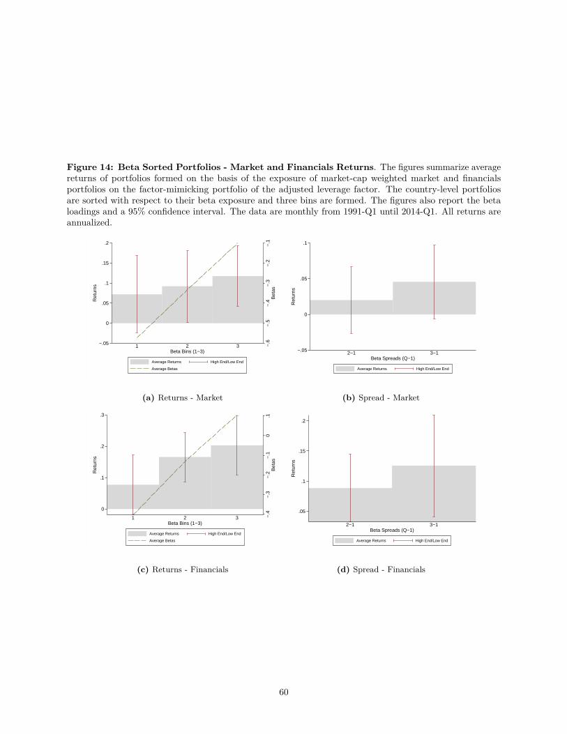
Figure 14: Beta Sorted Portfolios - Market and Financials Returns. The figures summarize averagereturns of portfolios formed on the basis of the exposure of market-cap weighted market and financialsportfolios on the factor-mimicking portfolio of the adjusted leverage factor. The country-level portfoliosare sorted with respect to their beta exposure and three bins are formed. The figures also report the betaloadings and a 95% confidence interval. The data are monthly from 1991-Q1 until 2014-Q1. All returns areannualized.

−.6

−.5

−.4

−.3

−.2

−.1

Bet

as

−.05

0

.05

.1

.15

.2

Ret

urns

1 2 3Beta Bins (1−3)

Average Returns High End/Low End

Average Betas

(a) Returns - Market

−.05

0

.05

.1

Ret

urns

2−1 3−1Beta Spreads (Q−1)

Average Returns High End/Low End

(b) Spread - Market

−.4

−.3

−.2

−.1

0.1

Bet

as

0

.1

.2

.3

Ret

urns

1 2 3Beta Bins (1−3)

Average Returns High End/Low End

Average Betas

(c) Returns - Financials

.05

.1

.15

.2

Ret

urns

2−1 3−1Beta Spreads (Q−1)

Average Returns High End/Low End

(d) Spread - Financials

60

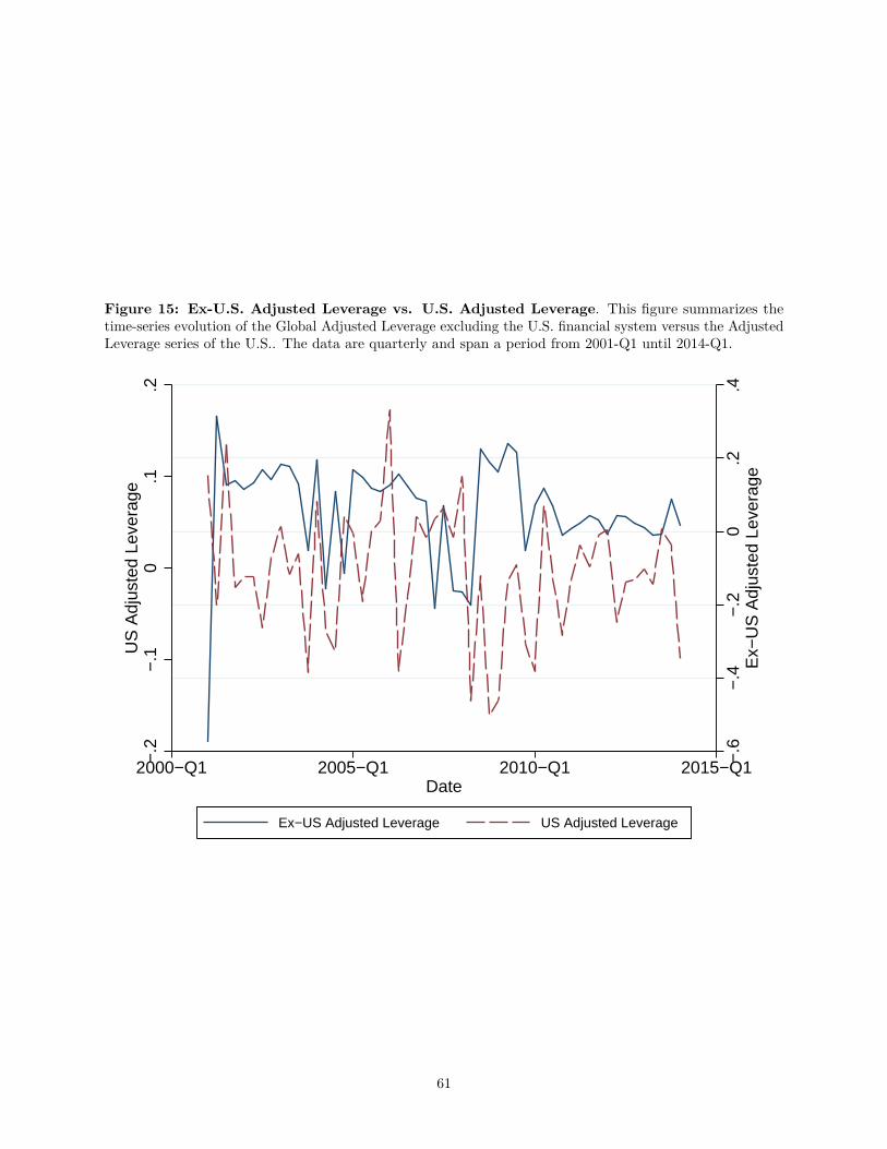
Figure 15: Ex-U.S. Adjusted Leverage vs. U.S. Adjusted Leverage. This figure summarizes thetime-series evolution of the Global Adjusted Leverage excluding the U.S. financial system versus the AdjustedLeverage series of the U.S.. The data are quarterly and span a period from 2001-Q1 until 2014-Q1.

−.2

−.1

0.1

.2U

S A

djus

ted

Leve

rage

−.6

−.4

−.2

0.2

.4E

x−U

S A

djus

ted

Leve

rage

2000−Q1 2005−Q1 2010−Q1 2015−Q1Date

Ex−US Adjusted Leverage US Adjusted Leverage

61

C Tables

Tab

le1:

Tim

elineof

theecon

omy.

The

tablesummarizes

thetim

elineof

thede

cisio

nsmad

eby

thethreeagents

ofthe

econ

omy(hou

seho

lds,

bank

s,an

dfirms).It

describ

esthede

cisio

nmak

ingprocessthat

takesplacein

perio

d1an

d2.

Period1

Period2

Hou

seho

ldan

dba

nkha

veform

edbe

liefs

regard-

ingthequ

ality

ofcolla

teral(p)an

deffi

cien

cyof

prod

uctio

n(q)

Firm

prod

uces

usingnu

meraire

(Kb)

Hou

seho

ldis

endo

wedwith

numeraire

(K)enou

gh

tosustainprod

uctio

n

Firm

repa

ysloan

toba

nk

Firm

appliesforaloan

from

theba

nkBan

kreceives

profi

tsfrom

firm

ownership(π

2)

Hou

seho

ldan

dba

nkde

cide

(sim

ultane

ously

)on

whe

ther

toprod

uceinform

ationat

acostγhan

d

γb,a

ndon

thelevelo

fdep

osit(K

h)an

dloan

(Kb)

Ban

krepa

ysloan

toho

useh

old

Firm

prod

uces

usingendo

wmentnu

meraire

(K1)

andba

nkreceives

proceeds

(π1)

Ban

kcolle

ctsland

output

(pC)

Ban

k,ho

useh

oldconsum

eforpe

riod1(cb,1,ch,1)

Ban

k,ho

useh

oldconsum

eforpe

riod2(cb,2,ch,2)

62

Table 2: Credit-to-Private Sector and Financial Leverage Data - Countries. The table summarizesthe countries for which data is available on credit-to-private sector and broker-dealers’ financial leverage.Data are quarterly from WorldScope and the World Development Indicators database; the start date is statedon the table, and the end date is Mar-2014.

Country Year Quarter Country Year Quarter1 Austria 2001 1 29 Malaysia 2005 42 Belgium 2001 4 30 Mexico 2001 13 Brazil 2004 3 31 Netherlands 2001 44 Bulgaria 2007 1 32 New Zealand 2005 15 Canada 1999 1 33 Norway 2001 16 Chile 2004 3 34 Oman 2004 37 Colombia 2004 3 35 Pakistan 2004 38 Croatia 2007 1 36 Peru 2004 39 Cyprus 2005 1 37 Philippines 2001 110 Czech Republic 2001 4 38 Poland 2002 411 Denmark 2001 1 39 Portugal 2001 112 Finland 2001 1 40 Qatar 2005 113 France 2002 1 41 Romania 2009 214 Germany 2001 1 42 Russian Federation 2005 115 Greece 2001 4 43 Saudi Arabia 2003 116 Hong Kong SAR, China 2001 4 44 Singapore 2002 217 Hungary 2002 4 45 Slovak Republic 2009 118 Iceland 2004 3 46 Slovenia 2009 119 India 2001 4 47 Spain 2001 120 Indonesia 2007 3 48 Sweden 2001 121 Israel 2004 3 49 Switzerland 2001 222 Italy 2001 1 50 Thailand 2001 123 Japan 2001 4 51 Ukraine 2006 124 Jordan 2004 3 52 United Arab Emirates 2003 225 Kazakhstan 2005 1 53 United Kingdom 2001 126 Kenya 2005 1 54 United States 1998 127 Korea (South) 2002 3 55 Venezuela 2004 328 Kuwait 2003 1

Table 3: Summary Statistics. The table summarizes descriptive statistics for the variables used in thepaper. The data are quarterly from 2001-Q1 until 2014-Q1.

Count Mean St.Dev Min MaxrGDP (in bn.) 568 1023.849 2293.663 11.408 16800INV (% of rGDP ) 551 22.808 4.850 13.008 46.811TFP 166 623.416 113.213 260.759 823.585Credit to Priv.(% of rGDP ) 573 87.873 53.368 15.499 241.044Credit to Corp.(% of rGDP ) 1435 80.318 35.197 11.800 211.600Credit to Hhld.(% of rGDP ) 1435 56.259 30.487 4.200 140.100Global Imbalances 297 -7.337 63.824 -127.637 252.845∆ rGDP 345 0.078 0.101 -0.264 0.329∆ INV 340 -0.003 0.081 -0.308 0.317∆ TFP 166 -0.002 0.026 -0.098 0.113∆Credit to Priv. 1334 0.006 0.028 -0.132 0.173∆Credit to Hhld. 1334 0.010 0.022 -0.097 0.167Financial Assets (in bn.) 2257 834.171 1589.500 0.040 8292.429Financial Leverage 2257 14.897 8.771 1.128 44.735Adjusted Leverage 2168 -0.003 0.229 -2.275 2.237Global Adjusted Leverage 64 0.010 0.136 -0.373 0.434Global F inancial Leverage Innovations 64 0 0.136 -0.434 0.345Currency Returns (Quarterly) 2257 0.422 4.639 -69.316 41.569Intermediaries′ Returns (Quarterly) 1459 0.340 0.735 -1.292 2.954

63

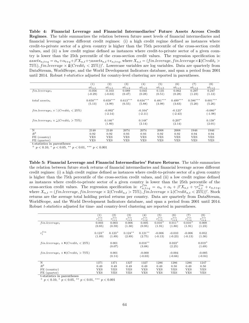
Table 4: Financial Leverage and Financial Intermediaries’ Future Assets Across CreditRegimes. The table summarizes the relation between future asset levels of financial intermediaries andfinancial leverage across different credit regimes: (i) a high credit regime defined as instances wherecredit-to-private sector of a given country is higher than the 75th percentile of the cross-section creditvalues, and (ii) a low credit regime defined as instances where credit-to-private sector of a given coun-try is lower than the 25th percentile of the cross-section credit values. The regression specification is:assetsn,t+q = αn+αt+q+β′Xn,t+γassetsn,t+εn,t+q, whereXn,t = (fin.leverage, fin.leverage×1(Creditt >75%), fin.leverage × 1(Creditt < 25%))′. Lowercase variables are log variables. Data are quarterly fromDataStream, WorldScope, and the World Development Indicators database, and span a period from 2001until 2014. Robust t-statistics adjusted for country-level clustering are reported in parentheses.

(1) (2) (3) (4) (5) (6) (7) (8)att+1 att+1 att+2 att+2 att+3 att+3 att+4 att+4

fin.leveraget -0.056 -0.103 0.089 0.045 0.135 0.062 0.297 0.247(-0.29) (-0.63) (0.47) (0.28) (0.51) (0.28) (1.23) (1.12)

total assetst 0.650∗∗∗ 0.659∗∗∗ 0.613∗∗∗ 0.634∗∗∗ 0.481∗∗∗ 0.499∗∗∗ 0.586∗∗∗ 0.601∗∗∗(5.13) (4.99) (6.55) (5.88) (3.99) (3.63) (5.20) (5.26)

fin.leveraget × 1(Creditt < 25%) -0.092∗ -0.104∗ -0.123∗ -0.080+

(-2.14) (-2.11) (-2.43) (-1.98)

fin.leveraget × 1(Creditt > 75%) 0.146+ 0.148∗ 0.207∗ 0.138∗(1.80) (2.14) (2.14) (2.01)

N 2148 2148 2074 2074 2008 2008 1946 1946R2 0.92 0.92 0.93 0.93 0.92 0.92 0.94 0.94FE (country) YES YES YES YES YES YES YES YESFE (quarter) YES YES YES YES YES YES YES YESt-statistics in parentheses+ p < 0.10, ∗ p < 0.05, ∗∗ p < 0.01, ∗∗∗ p < 0.001

Table 5: Financial Leverage and Financial Intermediaries’ Future Returns. The table summarizesthe relation between future stock returns of financial intermediaries and financial leverage across differentcredit regimes: (i) a high credit regime defined as instances where credit-to-private sector of a given countryis higher than the 75th percentile of the cross-section credit values, and (ii) a low credit regime definedas instances where credit-to-private sector of a given country is lower than the 25th percentile of thecross-section credit values. The regression specification is: rfinn,t+q = αn + αt + β′Xn,t + γrfinn,t + εn,t+q,where Xn,t = (fin.leverage, fin.leverage× 1(Creditn,t > 75%), fin.leverage× 1(Creditn,t < 25%))′. Stockreturns are the average total holding period returns per country. Data are quarterly from DataStream,WorldScope, and the World Development Indicators database, and span a period from 2001 until 2014.Robust t-statistics adjusted for time- and country-level clustering are reported in parentheses.

(1) (2) (3) (4) (5) (6) (7) (8)rfin

t+1 rfint+1 rfin

t+2 rfint+2 rfin

t+3 rfint+3 rfin

t+4 rfint+4

fin.leveraget 0.003 0.003 0.006 0.005 0.010+ 0.011+ 0.010+ 0.009(0.85) (0.59) (1.30) (0.95) (1.91) (1.80) (1.91) (1.23)

rfint 0.123+ 0.123+ 0.124∗∗ 0.121∗∗ -0.006 -0.010 -0.006 0.052

(1.89) (1.89) (2.89) (2.75) (-0.13) (-0.23) (-0.13) (1.30)

fin.leveraget × 1(Creditt < 25%) 0.001 0.016∗∗ 0.022∗ 0.019+

(0.07) (3.08) (2.25) (1.69)

fin.leveraget × 1(Creditt > 75%) 0.001 -0.000 -0.004 -0.005(0.14) (-0.03) (-0.66) (-0.84)

N 1371 1371 1327 1327 1286 1286 1286 1247R2 0.49 0.49 0.49 0.49 0.49 0.50 0.49 0.50FE (country) YES YES YES YES YES YES YES YESFE (quarter) YES YES YES YES YES YES YES YESt-statistics in parentheses+ p < 0.10, ∗ p < 0.05, ∗∗ p < 0.01, ∗∗∗ p < 0.001

64

Table 6: Adjusted Leverage and Macroeconomic Activity (U.S. Economy, Broker-Dealers). Thetable summarizes the explanatory power of global Adjusted Leverage (Adj.Lev) and leverage innovations(Lev.Inn) on logarithmic changes in household credit (HH.Cr), corporate credit (Corp.Cr), instances offinancial crises (Crisis), logarithmic changes in real GDP (rGDP ), capital formation (INV ), credit spread(Cr.Sprd), and total factor productivity (TFP ). The regression specification is: Economic V ariablen,t =αn + αt + βAdj.Levn,t + γLev.Innn,t + εn,t, where Economic V ariablen,t = (HH.Crn,t, Corp.Crn,t,rGDP , INV , Cr.Sprdn,t, TFPn,t), and Pr(Crisisn,t = 1|Xn,t) = 1/(1 + e−(αn+β′Xn,t)), where Xn,t =(Adj.Levn,t, Lev.Innn,t). Data are quarterly from WorldScope, World Development Indicators, and Valenciaand Laeven (2012) and span a period from 2001 until 2014. Standard errors are heteroskedasticity- (White(1980)) and autocorrelation-robust (Newey and West (1987) and Newey and West (1994)).

(1) (2) (3) (4) (5) (6) (7)HH.Cr Corp.Cr Crisis rGDP INV Cr.Sprd TFP

Adj.Levt 0.033∗∗∗ -0.001 -23.271∗ 0.118∗∗ 0.467∗ -1.185∗ 0.188∗∗(6.06) (-0.12) (-2.11) (3.43) (2.63) (-2.58) (4.73)

Lev.Innt 0.062∗∗∗ 0.021 -8.188 0.167∗∗∗ 0.101 0.402 0.057(5.28) (1.05) (-0.78) (4.65) (0.94) (0.67) (1.10)

N 53 53 40 13 12 39 10R2 0.28 0.05 0.51 0.44 0.06 0.61t-statistics in parentheses+ p < 0.10, ∗ p < 0.05, ∗∗ p < 0.01, ∗∗∗ p < 0.001

Table 7: Adjusted Leverage and Financial Crises. The table summarizes the predictive powerof country level Adjusted Leverage on Financial Crises. The regression specification is: (A) a lin-ear probability model (columns (1) and (2)): 1(Crisisn,t) = αn + β′Xn,t + εn,t, and (B) a logitmodel (columns (3) and (4)): Pr(Crisisn,t = 1|Xn,t) = 1/(1 + e−(αn+β′Xn,t)), where Xn,t =(Adj.Levn,t, Adj.Levn,t−1, Adj.Levn,t−2, Creditn,t, Creditn,t−1, Creditn,t−2). Data are from WorldScope,World Development Indicators, and Valencia and Laeven (2012) and span a period from 2001 until 2014.

(1) (2) (3) (4)LPM LPM LOGIT LOGIT

Adj.Levt 0.012 0.009 0.042 -3.605(0.07) (0.07) (0.05) (-0.99)

Adj.Levt−1 0.006 0.068 -0.041 -4.408(0.05) (1.04) (-0.05) (-0.83)

Adj.Levt−2 -0.189∗ -0.113+ -1.231 -10.664+

(-2.02) (-1.76) (-1.37) (-1.74)

Creditt -0.005 -0.002 -0.025 0.329(-0.66) (-0.30) (-0.63) (0.97)

Creditt−1 0.009 0.007 0.043 0.356(0.72) (1.19) (0.72) (1.37)

Creditt−2 -0.001 0.017∗∗∗ -0.003 0.723+

(-0.14) (4.73) (-0.09) (1.86)

N 113 113 113 78R2 0.13 0.60FE (country) NO YES NO YESt-statistics in parentheses+ p < 0.10, ∗ p < 0.05, ∗∗ p < 0.01, ∗∗∗ p < 0.001

65

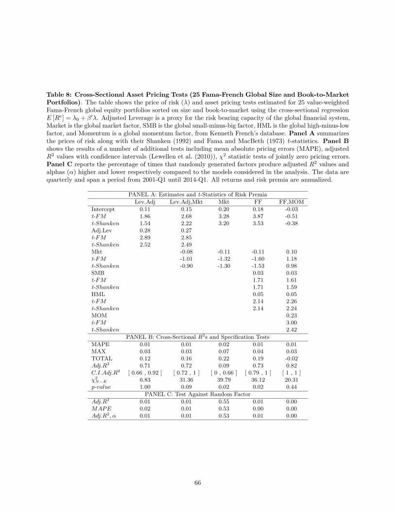
Table 8: Cross-Sectional Asset Pricing Tests (25 Fama-French Global Size and Book-to-MarketPortfolios). The table shows the price of risk (λ) and asset pricing tests estimated for 25 value-weightedFama-French global equity portfolios sorted on size and book-to-market using the cross-sectional regressionE [Re] = λ0 + β′λ. Adjusted Leverage is a proxy for the risk bearing capacity of the global financial system,Market is the global market factor, SMB is the global small-minus-big factor, HML is the global high-minus-lowfactor, and Momentum is a global momentum factor, from Kenneth French’s database. Panel A summarizesthe prices of risk along with their Shanken (1992) and Fama and MacBeth (1973) t-statistics. Panel Bshows the results of a number of additional tests including mean absolute pricing errors (MAPE), adjustedR2 values with confidence intervals (Lewellen et al. (2010)), χ2 statistic tests of jointly zero pricing errors.Panel C reports the percentage of times that randomly generated factors produce adjusted R2 values andalphas (α) higher and lower respectively compared to the models considered in the analysis. The data arequarterly and span a period from 2001-Q1 until 2014-Q1. All returns and risk premia are annualized.

PANEL A: Estimates and t-Statistics of Risk PremiaLev.Adj Lev.Adj,Mkt Mkt FF FF,MOM

Intercept 0.11 0.15 0.20 0.18 -0.03t-FM 1.86 2.68 3.28 3.87 -0.51t-Shanken 1.54 2.22 3.20 3.53 -0.38Adj.Lev 0.28 0.27t-FM 2.89 2.85t-Shanken 2.52 2.49Mkt -0.08 -0.11 -0.11 0.10t-FM -1.01 -1.32 -1.60 1.18t-Shanken -0.90 -1.30 -1.53 0.98SMB 0.03 0.03t-FM 1.71 1.61t-Shanken 1.71 1.59HML 0.05 0.05t-FM 2.14 2.26t-Shanken 2.14 2.24MOM 0.23t-FM 3.00t-Shanken 2.42

PANEL B: Cross-Sectional R2s and Specification TestsMAPE 0.01 0.01 0.02 0.01 0.01MAX 0.03 0.03 0.07 0.04 0.03TOTAL 0.12 0.16 0.22 0.19 -0.02Adj.R2 0.71 0.72 0.09 0.73 0.82C.I.Adj.R2 [ 0.66 , 0.92 ] [ 0.72 , 1 ] [ 0 , 0.66 ] [ 0.79 , 1 ] [ 1 , 1 ]χ2N−K 6.83 31.36 39.79 36.12 20.31

p-value 1.00 0.09 0.02 0.02 0.44PANEL C: Test Against Random Factor

Adj.R2 0.01 0.01 0.55 0.01 0.00MAPE 0.02 0.01 0.53 0.00 0.00Adj.R2, α 0.01 0.01 0.53 0.01 0.00

66

Table 9: Cross-Sectional Asset Pricing Tests (25 Fama-French Global Size and MomentumPortfolios). The table shows the price of risk (λ) and asset pricing tests estimated for 25 value-weightedFama-French global equity portfolios sorted on size and momentum using the cross-sectional regressionE [Re] = λ0 + β′λ. Adjusted Leverage is a proxy for the risk bearing capacity of the global financial system,Market is the global market factor, SMB is the global small-minus-big factor, HML is the global high-minus-lowfactor, and Momentum is a global momentum factor, from Kenneth French’s database. Panel A summarizesthe prices of risk along with their Shanken (1992) and Fama and MacBeth (1973) t-statistics. Panel Bshows the results of a number of additional tests including mean absolute pricing errors (MAPE), adjustedR2 values with confidence intervals (Lewellen et al. (2010)), χ2 statistic tests of jointly zero pricing errors.Panel C reports the percentage of times that randomly generated factors produce adjusted R2 values andalphas (α) higher and lower respectively compared to the models considered in the analysis. The data arequarterly and span a period from 2001-Q1 until 2014-Q1. All returns and risk premia are annualized.

PANEL A: Estimates and t-Statistics of Risk PremiaLev.Adj Lev.Adj,Mkt Mkt FF FF,MOM

Intercept 0.12 0.14 0.18 0.19 0.05t-FM 2.23 1.91 2.50 2.32 1.08t-Shanken 1.61 1.40 2.47 2.08 0.96Adj.Lev 0.39 0.37t-FM 2.84 3.54t-Shanken 2.13 2.77Mkt -0.07 -0.08 -0.12 0.01t-FM -0.77 -0.86 -1.28 0.22t-Shanken -0.62 -0.86 -1.18 0.21SMB 0.04 0.05t-FM 2.14 2.58t-Shanken 2.10 2.54HML 0.04 0.06t-FM 1.05 1.41t-Shanken 0.98 1.30MOM 0.05t-FM 1.23t-Shanken 1.22

PANEL B: Cross-Sectional R2s and Specification TestsMAPE 0.01 0.01 0.02 0.02 0.01MAX 0.04 0.04 0.09 0.06 0.04TOTAL 0.14 0.15 0.20 0.21 0.06Adj.R2 0.75 0.75 0.18 0.62 0.81C.I.Adj.R2 [ 0.71 , 0.93 ] [ 0.79 , 1 ] [ 0 , 0.72 ] [ 0.56 , 1 ] [ 0.98 , 1 ]χ2N−K 1.88 12.71 34.14 33.71 26.43

p-value 1.00 0.94 0.06 0.04 0.15PANEL C: Test Against Random Factor

Adj.R2 0.01 0.01 0.45 0.04 0.00MAPE 0.01 0.01 0.33 0.03 0.00Adj.R2, α 0.01 0.01 0.42 0.04 0.00

67

Table 10: Cross-Sectional Asset Pricing Tests (Currency Portfolios). The table shows the priceof risk (λ) and asset pricing tests estimated for 6 carry trade portfolios, 6 currency momentum portfolios(short-term), 6 currency momentum portfolios (long-term), and 6 currency value portfolios using the cross-sectional regression E [Re] = λ0 +β′λ. Adjusted Leverage is a proxy for the risk bearing capacity of the globalfinancial system, Carry is the carry trade portfolio, Volatility is the global 1/V ol measure, and Momentum is along/short portfolio on currency momentum. Panel A summarizes the prices of risk along with their Shanken(1992) and Fama and MacBeth (1973) t-statistics. Panel B shows the results of a number of additionaltests including mean absolute pricing errors (MAPE), adjusted R2 values with confidence intervals (Lewellenet al. (2010)), χ2 statistic tests of jointly zero pricing errors. Panel C reports the percentage of timesthat randomly generated factors produce adjusted R2 values and alphas (α) higher and lower respectivelycompared to the models considered in the analysis. The data are quarterly and span a period from 2001-Q1until 2014-Q1. All returns and risk premia are annualized.

PANEL A: Estimates and t-Statistics of Risk PremiaLev.Adj Lev.Adj,CAR CAR VOL MOM

Intercept 0.11 0.10 0.00 0.08 0.02t-FM 5.53 5.44 0.17 4.43 1.17t-Shanken 1.29 1.30 0.16 2.69 0.87LEV.Adj 1.66 1.61t-FM 8.11 7.46t-Shanken 1.95 1.84CAR 0.11 0.09t-FM 4.08 3.31t-Shanken 2.03 3.24VOL 0.31t-FM 4.28t-Shanken 2.77MOM 0.19t-FM 5.75t-Shanken 5.22

PANEL B: Cross-Sectional R2s and Specification TestsMAPE 0.03 0.03 0.04 0.04 0.03MAX 0.09 0.09 0.13 0.13 0.08TOTAL 0.14 0.13 0.04 0.12 0.05Adj.R2 0.53 0.52 0.05 0.20 0.47C.I.Adj.R2 [ 0.43 , 0.86 ] [ 0.41 , 1 ] [ 0.03 , 0.63 ] [ 0.01 , 0.72 ] [ 0.36 , 0.84 ]χ2N−K 6.24 9.56 101.82 55.74 34.85

p-value 1.00 0.98 0.00 0.00 0.04PANEL C: Test Against Random Factor

Adj.R2 0.12 0.12 0.65 0.43 0.16MAPE 0.17 0.16 0.46 0.45 0.15Adj.R2, α 0.11 0.11 0.17 0.37 0.07

68

Tab

le11

:Cross-Section

alAsset

Pricing

Tests

(Portfoliosof

Internationa

lAssets)

-Fa

ctor-M

imicking

Portfolio.The

tableshow

sthe

priceof

risk(λ)an

dassetpricingtestsestim

ated

forinternationa

lportfolios(SizeandBook-to-Market,S

izeandMom

entum,a

ndCurrencies)

usingthecross-sectiona

lregressionE

[Re]=

λ0

+β′ λ.AdjustedLe

verage

isthefactor-m

imicking

portfolio

oftheglob

alad

justed

leverage

factor,

Marketis

theglob

almarketfactor,S

MB

istheglob

alsm

all-m

inus-big

factor,H

MLis

theglob

alhigh

-minus-lo

wfactor,a

ndMom

entum

isaglob

almom

entum

factor,from

Ken

neth

Fren

ch’s

databa

se.Pan

elA

summarizes

theprices

ofris

kalon

gwith

theirSh

anken(199

2)an

dFa

maan

dMacBeth

(197

3)t-statist

ics.Pan

elB

show

stheresults

ofanu

mbe

rof

additio

naltests

includ

ingmeanab

solute

pricingerrors

(MAPE

),ad

justed

R2values

with

confi

denc

eintervals(L

ewellenet

al.(20

10)),χ

2statist

ictestsof

jointly

zero

pricingerrors.Pan

elC

repo

rtsthepe

rcentage

oftim

esthat

rand

omly

gene

ratedfactorsprod

ucead

justed

R2values

andalph

as(α

)high

eran

dlower

respectiv

elycompa

redto

themod

elsconsidered

inthean

alysis.

The

data

arequ

arterly

,Tab

le11aspan

sape

riodfrom

1991-Q

1un

til2014-Q

1,an

dTa

ble11bspan

sape

riodfrom

2001-Q

1un

til20

14-Q

1.Allreturnsan

dris

kprem

iaarean

nualized

. (a)1991Q1-2014Q1

PANEL

A:E

stim

ates

andt-Statist

icsof

Risk

Prem

iaSM

BSM

OM

CUR

Intercep

t0.09

0.08

0.01

t-FM

2.49

1.97

0.55

t-Shanken

2.43

1.97

0.19

Adj.Lev

0.07

-0.04

0.78

t-FM

2.20

-0.77

9.77

t-Shanken

2.19

-0.77

3.72

PANEL

B:C

ross-Sectio

nalR

2 san

dSp

ecificatio

nTe

sts

MAPE

0.01

0.03

0.02

MAX

0.04

0.11

0.06

TOTA

L0.10

0.11

0.03

Adj.R

20.68

-0.01

0.72

C.I.Adj.R

2[0

.59,0

.91]

[0,0

.54]

[0.66,0

.92]

χ2 N−K

10.49

25.61

7.77

p-value

0.99

0.32

1.00

PANEL

C:T

estAgainst

Ran

dom

Factor

Adj.R

20.01

0.84

0.01

MAPE

0.01

0.84

0.01

Adj.R

2 ,α

0.01

0.30

0.01

(b)2001Q1-2014Q1

PANEL

A:E

stim

ates

andt-Statist

icsof

Risk

Prem

iaSM

BSM

OM

CUR

Intercep

t0.11

0.13

0.03

t-FM

1.85

2.33

1.47

t-Shanken

1.73

1.94

0.81

Adj.Lev

0.10

0.16

0.37

t-FM

2.79

2.84

6.02

t-Shanken

2.75

2.49

3.71

PANEL

B:C

ross-Sectio

nalR

2 san

dSp

ecificatio

nTe

sts

MAPE

0.01

0.01

0.03

MAX

0.04

0.05

0.11

TOTA

L0.12

0.14

0.06

Adj.R

20.69

0.74

0.48

C.I.Adj.R

2[0

.63,0

.91]

[0.69,0

.93]

[0.36,0

.85]

χ2 N−K

9.32

2.54

18.74

p-value

0.99

1.00

0.66

PANEL

C:T

estAgainst

Ran

dom

Factor

Adj.R

20.02

0.01

0.16

MAPE

0.01

0.01

0.15

Adj.R

2 ,α

0.01

0.01

0.08

69

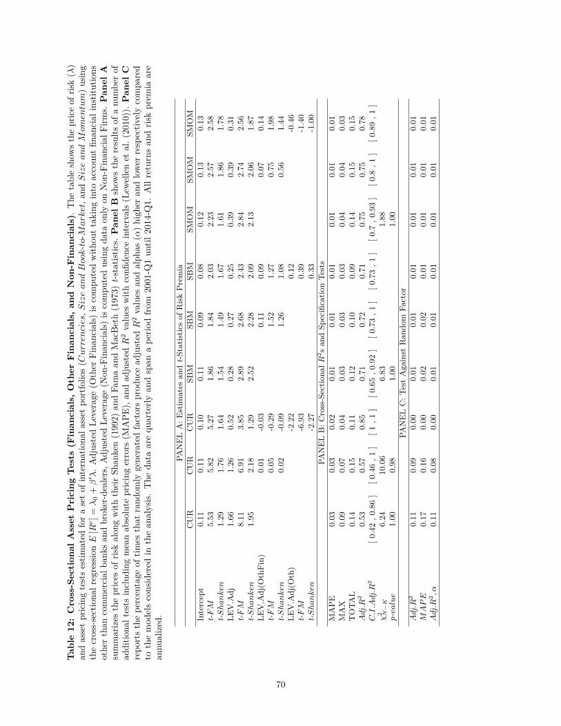
Tab

le12

:Cross-Section

alAsset

Pricing

Tests

(Finan

cials,

Other

Finan

cials,

andNon

-Finan

cials).The

tableshow

sthepriceof

risk(λ)

andassetpricingtestsestim

ated

forasetof

internationa

lasset

portfolio

s(Currencies,SizeandBook-to-Market,a

ndSizeandMom

entum)using

thecross-sectiona

lregressionE

[Re]=

λ0

+β′ λ.AdjustedLe

verage

(Other

Fina

ncials)

iscompu

tedwith

outtaking

into

accoun

tfin

ancial

institu

tions

othe

rthan

commercial

bank

san

dbroker-dealers,A

djustedLe

verage

(Non

-Finan

cials)

iscompu

tedusingda

taon

lyon

Non

-Finan

cial

Firm

s.Pan

elA

summarizes

theprices

ofris

kalon

gwith

theirSh

anken(1992)

andFa

maan

dMacBeth(1973)

t-statist

ics.Pan

elB

show

stheresults

ofanu

mbe

rof

additio

nalt

ests

includ

ingmeanab

solute

pricingerrors

(MAPE

),an

dad

justed

R2values

with

confi

denc

eintervals(L

ewellenet

al.(

2010)).Pan

elC

repo

rtsthepe

rcentage

oftim

esthat

rand

omly

generatedfactorsprod

ucead

justed

R2values

andalph

as(α

)high

eran

dlower

respectiv

elycompa

red

tothemod

elsconsidered

inthean

alysis.

The

data

arequ

arterly

andspan

ape

riodfrom

2001

-Q1un

til2014

-Q1.

Allreturnsan

dris

kprem

iaare

annu

alized

.

PANELA:E

stim

ates

and

t-Statistic

sof

RiskPremia

CUR

CUR

CUR

SBM

SBM

SBM

SMOM

SMOM

SMOM

Intercep

t0.11

0.11

0.10

0.11

0.09

0.08

0.12

0.13

0.13

t-FM

5.53

5.82

5.27

1.86

1.84

2.03

2.23

2.57

2.58

t-Shanken

1.29

1.76

1.64

1.54

1.49

1.67

1.61

1.86

1.78

LEV.Adj

1.66

1.26

0.52

0.28

0.27

0.25

0.39

0.39

0.31

t-FM

8.11

6.91

3.85

2.89

2.68

2.43

2.84

2.74

2.56

t-Shanken

1.95

2.18

1.29

2.52

2.28

2.09

2.13

2.06

1.87

LEV.Adj(O

thFin)

0.01

-0.03

0.11

0.09

0.07

0.14

t-FM

0.05

-0.29

1.52

1.27

0.75

1.98

t-Shanken

0.02

-0.09

1.26

1.08

0.56

1.44

LEV.Adj(O

th)

-2.22

0.12

-0.46

t-FM

-6.93

0.39

-1.40

t-Shanken

-2.27

0.33

-1.00

PANELB:C

ross-Sectio

nalR

2san

dSp

ecificatio

nTe

sts

MAPE

0.03

0.03

0.02

0.01

0.01

0.01

0.01

0.01

0.01

MAX

0.09

0.07

0.04

0.03

0.03

0.03

0.04

0.04

0.03

TOTA

L0.14

0.15

0.11

0.12

0.10

0.09

0.14

0.15

0.15

Adj.R

20.53

0.57

0.85

0.71

0.72

0.71

0.75

0.75

0.78

C.I.Adj.R

2[0

.42,0

.86]

[0.46,1

][1

,1]

[0.65,0

.92]

[0.73,1

][0

.73,1

][0

.7,0

.93]

[0.8

,1]

[0.89,1

]χ

2 N−K

6.24

10.06

6.83

1.88

p-value

1.00

0.98

1.00

1.00

PANELC:T

estAgainst

Ran

dom

Factor

Adj.R

20.11

0.09

0.00

0.01

0.01

0.01

0.01

0.01

0.01

MAPE

0.17

0.16

0.00

0.02

0.02

0.01

0.01

0.01

0.01

Adj.R

2,α

0.11

0.08

0.00

0.01

0.01

0.01

0.01

0.01

0.01

70

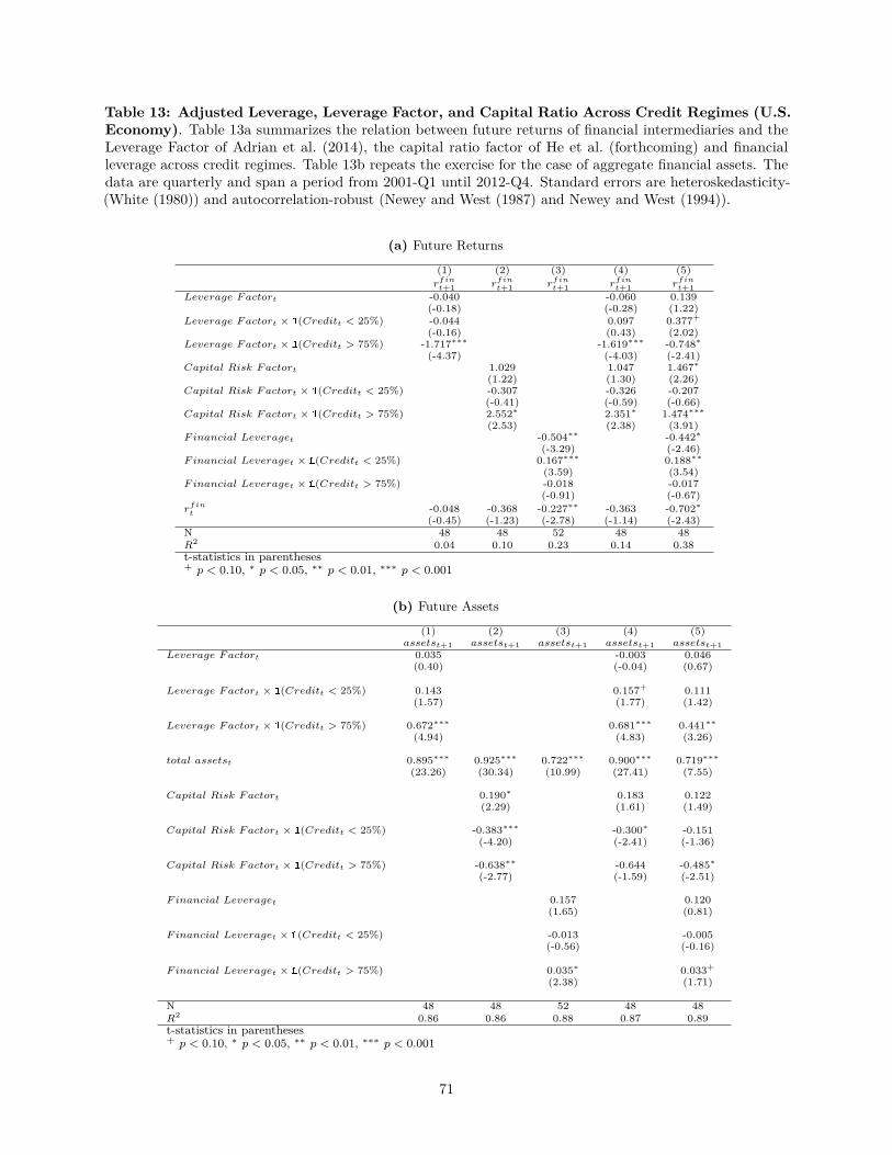
Table 13: Adjusted Leverage, Leverage Factor, and Capital Ratio Across Credit Regimes (U.S.Economy). Table 13a summarizes the relation between future returns of financial intermediaries and theLeverage Factor of Adrian et al. (2014), the capital ratio factor of He et al. (forthcoming) and financialleverage across credit regimes. Table 13b repeats the exercise for the case of aggregate financial assets. Thedata are quarterly and span a period from 2001-Q1 until 2012-Q4. Standard errors are heteroskedasticity-(White (1980)) and autocorrelation-robust (Newey and West (1987) and Newey and West (1994)).

(a) Future Returns

(1) (2) (3) (4) (5)rfin

t+1 rfint+1 rfin

t+1 rfint+1 rfin

t+1Leverage Factort -0.040 -0.060 0.139

(-0.18) (-0.28) (1.22)Leverage Factort × 1(Creditt < 25%) -0.044 0.097 0.377+

(-0.16) (0.43) (2.02)Leverage Factort × 1(Creditt > 75%) -1.717∗∗∗ -1.619∗∗∗ -0.748∗

(-4.37) (-4.03) (-2.41)Capital Risk Factort 1.029 1.047 1.467∗

(1.22) (1.30) (2.26)Capital Risk Factort × 1(Creditt < 25%) -0.307 -0.326 -0.207

(-0.41) (-0.59) (-0.66)Capital Risk Factort × 1(Creditt > 75%) 2.552∗ 2.351∗ 1.474∗∗∗

(2.53) (2.38) (3.91)Financial Leveraget -0.504∗∗ -0.442∗

(-3.29) (-2.46)Financial Leveraget × 1(Creditt < 25%) 0.167∗∗∗ 0.188∗∗

(3.59) (3.54)Financial Leveraget × 1(Creditt > 75%) -0.018 -0.017

(-0.91) (-0.67)rfin

t -0.048 -0.368 -0.227∗∗ -0.363 -0.702∗(-0.45) (-1.23) (-2.78) (-1.14) (-2.43)

N 48 48 52 48 48R2 0.04 0.10 0.23 0.14 0.38t-statistics in parentheses+ p < 0.10, ∗ p < 0.05, ∗∗ p < 0.01, ∗∗∗ p < 0.001

(b) Future Assets

(1) (2) (3) (4) (5)assetst+1 assetst+1 assetst+1 assetst+1 assetst+1

Leverage Factort 0.035 -0.003 0.046(0.40) (-0.04) (0.67)

Leverage Factort × 1(Creditt < 25%) 0.143 0.157+ 0.111(1.57) (1.77) (1.42)

Leverage Factort × 1(Creditt > 75%) 0.672∗∗∗ 0.681∗∗∗ 0.441∗∗(4.94) (4.83) (3.26)

total assetst 0.895∗∗∗ 0.925∗∗∗ 0.722∗∗∗ 0.900∗∗∗ 0.719∗∗∗(23.26) (30.34) (10.99) (27.41) (7.55)

Capital Risk Factort 0.190∗ 0.183 0.122(2.29) (1.61) (1.49)

Capital Risk Factort × 1(Creditt < 25%) -0.383∗∗∗ -0.300∗ -0.151(-4.20) (-2.41) (-1.36)

Capital Risk Factort × 1(Creditt > 75%) -0.638∗∗ -0.644 -0.485∗(-2.77) (-1.59) (-2.51)

Financial Leveraget 0.157 0.120(1.65) (0.81)

Financial Leveraget × 1(Creditt < 25%) -0.013 -0.005(-0.56) (-0.16)

Financial Leveraget × 1(Creditt > 75%) 0.035∗ 0.033+

(2.38) (1.71)

N 48 48 52 48 48R2 0.86 0.86 0.88 0.87 0.89t-statistics in parentheses+ p < 0.10, ∗ p < 0.05, ∗∗ p < 0.01, ∗∗∗ p < 0.001

71

Table 14: Cross-Sectional Asset Pricing Tests (Portfolios of International Assets). The tableshows the price of risk (λ) and asset pricing tests estimated for a set of International asset portfolios(Currencies, Size and Book-to-Market, and Size and Momentum) using the cross-sectional regressionE [Re] = λ0 + β′λ. Adjusted Leverage is a proxy for the risk bearing capacity of the global financial system,HKM is the intermediary capital factor of He et al. (forthcoming), and AEM is the leverage factor of Adrianet al. (2014). Panel A summarizes the prices of risk along with their Shanken (1992) and Fama and MacBeth(1973) t-statistics. Panel B shows the results of a number of additional tests including mean absolute pricingerrors (MAPE), adjusted R2 values with confidence intervals (Lewellen et al. (2010)), χ2 statistic tests ofjointly zero pricing errors. Panel C reports the percentage of times that randomly generated factors produceadjusted R2 values and alphas (α) higher and lower respectively compared to the models considered in theanalysis. The data are quarterly and span a period from 2001-Q1 until 2012-Q4. All returns and risk premiaare annualized.

PANEL A: Estimates and t-Statistics of Risk PremiaCUR SBM SMOM

Intercept 0.11 0.15 0.08t-FM 5.28 2.80 1.77t-Shanken 1.88 2.23 1.39LEV.Adj 0.90 0.29 0.30t-FM 6.21 2.99 3.00t-Shanken 2.38 2.55 2.53HKM -0.55 -0.13 -0.04t-FM -4.43 -1.31 -0.30t-Shanken -2.00 -1.19 -0.26AEM -47.47 -6.07 -13.65t-FM -2.94 -0.27 -0.73t-Shanken -1.17 -0.22 -0.60PANEL B: Cross-Sectional R2s and Specification TestsMAPE 0.03 0.01 0.01MAX 0.07 0.05 0.03TOTAL 0.14 0.16 0.09Adj.R2 0.58 0.69 0.81C.I.Adj.R2 [ 0.5 , 1 ] [ 0.68 , 0.98 ] [ 0.98 , 1 ]

PANEL C: Test Against Random FactorAdj.R2 0.09 0.01 0.00MAPE 0.14 0.01 0.00Adj.R2, α 0.08 0.01 0.00

72

Table 15: Cross-Sectional Asset Pricing Tests (Portfolios of International Assets). The tableshows the price of risk (λ) and asset pricing tests estimated for a set of international asset portfolios(Currencies, Size and Book-to-Market, and Size and Momentum) using the cross-sectional regressionE [Re] = λ0 + β′λ. Adjusted Leverage is a proxy for the risk bearing capacity of the global financial systemand Leverage Innovations are the residuals of an AR(1) regression of global financial leverage. Panel Asummarizes the prices of risk along with their Shanken (1992) and Fama and MacBeth (1973) t-statistics.Panel B shows the results of a number of additional tests including mean absolute pricing errors (MAPE),and adjusted R2 values with confidence intervals (Lewellen et al. (2010)). Panel C reports the percentageof times that randomly generated factors produce adjusted R2 values and alphas (α) higher and lowerrespectively compared to the models considered in the analysis. The data are quarterly and span a periodfrom 2001-Q1 until 2014-Q1. All returns and risk premia are annualized.

PANEL A: Estimates and t-Statistics of Risk PremiaSBM SBM SMOM SMOM CUR CUR

Intercept 0.11 0.12 0.12 0.12 0.12 0.10t-FM 1.86 1.96 2.23 1.99 5.48 4.99t-Shanken 1.54 1.47 1.61 1.44 1.28 0.97Adj.Lev 0.28 0.27 0.39 0.39 1.66 1.89t-FM 2.89 2.80 2.84 2.02 8.11 8.12t-Shanken 2.52 2.27 2.13 1.49 1.95 1.62Lev.Inn 0.22 -0.02 0.61t-FM 1.81 -0.03 4.33t-Shanken 1.42 -0.02 0.91

PANEL B: Cross-Sectional R2s and Specification TestsMAPE 0.01 0.01 0.01 0.01 0.03 0.03MAX 0.03 0.02 0.04 0.04 0.09 0.07TOTAL 0.12 0.13 0.14 0.14 0.15 0.13Adj.R2 0.71 0.81 0.75 0.74 0.53 0.61C.I.Adj.R2 [ 0.64 , 0.92 ] [ 0.93 , 1 ] [ 0.7 , 0.93 ] [ 0.79 , 1 ] [ 0.43 , 0.86 ] [ 0.53 , 1 ]χ2N−K 6.83 4.52 1.88 -0.10 7.33 11.48

p-value 1.00 1.00 1.00 1.00 1.00 0.95PANEL C: Test Against Random Factor

Adj.R2 0.01 0.00 0.01 0.01 0.12 0.07MAPE 0.02 0.00 0.01 0.01 0.17 0.08Adj.R2, α 0.01 0.00 0.01 0.01 0.12 0.07

73

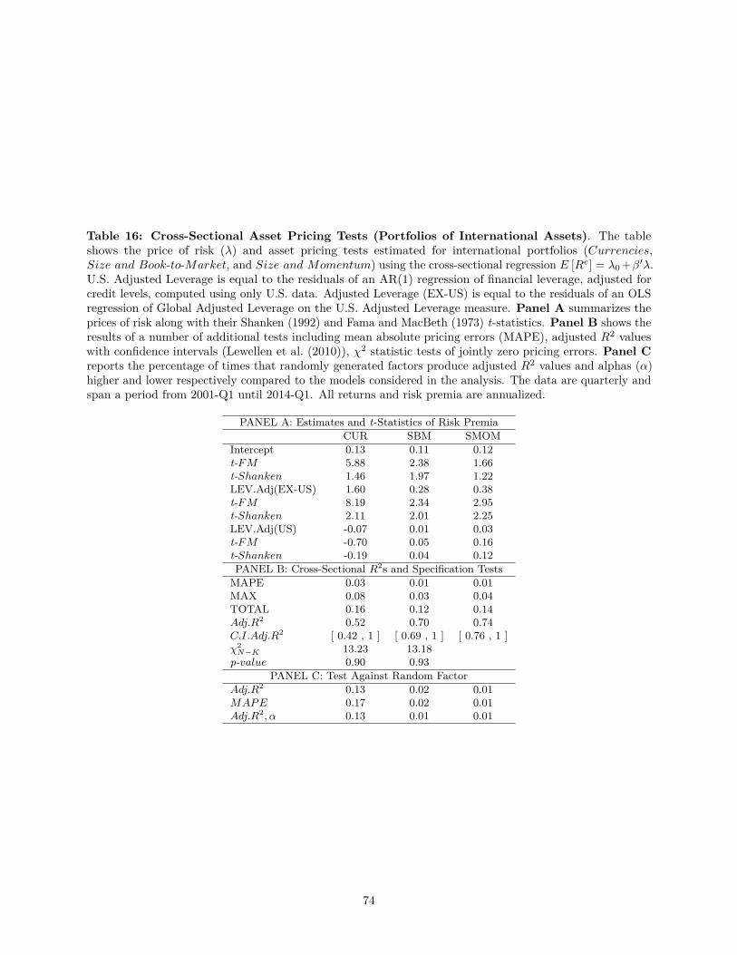
Table 16: Cross-Sectional Asset Pricing Tests (Portfolios of International Assets). The tableshows the price of risk (λ) and asset pricing tests estimated for international portfolios (Currencies,Size and Book-to-Market, and Size and Momentum) using the cross-sectional regression E [Re] = λ0 +β′λ.U.S. Adjusted Leverage is equal to the residuals of an AR(1) regression of financial leverage, adjusted forcredit levels, computed using only U.S. data. Adjusted Leverage (EX-US) is equal to the residuals of an OLSregression of Global Adjusted Leverage on the U.S. Adjusted Leverage measure. Panel A summarizes theprices of risk along with their Shanken (1992) and Fama and MacBeth (1973) t-statistics. Panel B shows theresults of a number of additional tests including mean absolute pricing errors (MAPE), adjusted R2 valueswith confidence intervals (Lewellen et al. (2010)), χ2 statistic tests of jointly zero pricing errors. Panel Creports the percentage of times that randomly generated factors produce adjusted R2 values and alphas (α)higher and lower respectively compared to the models considered in the analysis. The data are quarterly andspan a period from 2001-Q1 until 2014-Q1. All returns and risk premia are annualized.

PANEL A: Estimates and t-Statistics of Risk PremiaCUR SBM SMOM

Intercept 0.13 0.11 0.12t-FM 5.88 2.38 1.66t-Shanken 1.46 1.97 1.22LEV.Adj(EX-US) 1.60 0.28 0.38t-FM 8.19 2.34 2.95t-Shanken 2.11 2.01 2.25LEV.Adj(US) -0.07 0.01 0.03t-FM -0.70 0.05 0.16t-Shanken -0.19 0.04 0.12PANEL B: Cross-Sectional R2s and Specification TestsMAPE 0.03 0.01 0.01MAX 0.08 0.03 0.04TOTAL 0.16 0.12 0.14Adj.R2 0.52 0.70 0.74C.I.Adj.R2 [ 0.42 , 1 ] [ 0.69 , 1 ] [ 0.76 , 1 ]χ2N−K 13.23 13.18

p-value 0.90 0.93PANEL C: Test Against Random Factor

Adj.R2 0.13 0.02 0.01MAPE 0.17 0.02 0.01Adj.R2, α 0.13 0.01 0.01

74