financial intermediation and credit policy in business ... · financial intermediation and credit...
TRANSCRIPT
Financial Intermediation and Credit Policy
In
Business Cycle Analysis
Mark Gertler and Nobuhiro Kiyotaki
NYU and Princeton
October 20090

Old Motivation (for BGG 1999)
• Great Depression
• Emerging market crises over the past quarter century
.
1

New Motivation (for GK 2009)
• Global economy during Bernanke’s tenure as Fed Chair
2
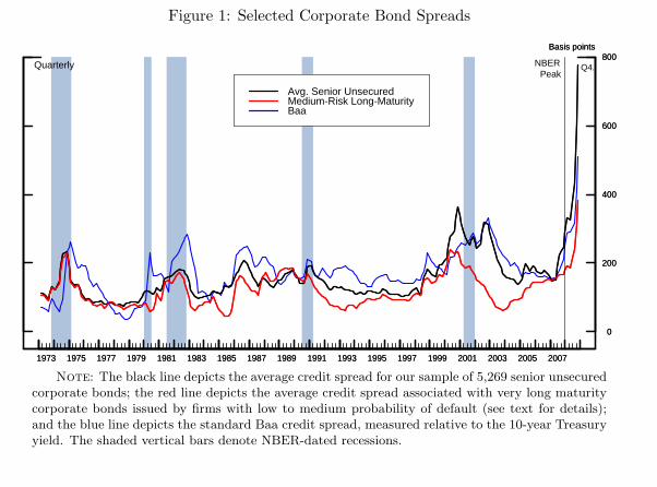
Figure 1: Selected Corporate Bond Spreads
1973 1975 1977 1979 1981 1983 1985 1987 1989 1991 1993 1995 1997 1999 2001 2003 2005 2007
0
200
400
600
800Basis points
1973 1975 1977 1979 1981 1983 1985 1987 1989 1991 1993 1995 1997 1999 2001 2003 2005 2007
0
200
400
600
800Basis points
Avg. Senior UnsecuredMedium-Risk Long-MaturityBaa
Quarterly Q4.NBERPeak
Note: The black line depicts the average credit spread for our sample of 5,269 senior unsecuredcorporate bonds; the red line depicts the average credit spread associated with very long maturitycorporate bonds issued by firms with low to medium probability of default (see text for details);and the blue line depicts the standard Baa credit spread, measured relative to the 10-year Treasuryyield. The shaded vertical bars denote NBER-dated recessions.
37
1990 1992 1994 1996 1998 2000 2002 2004 2006 2008−100
−50
0
50
100
1990 1992 1994 1996 1998 2000 2002 2004 2006 2008−0.02
−0.01
0
0.01
0.02
lending standards (left)
real GDP growth (right)

Challenges for Writing a Handbook Chapter
• Much of the relevant literature predates August 2007
• Most of the work afterwards is still in preliminary working paper form.
3

Our Approach: Look both Forward and Backward
• Present Canonical Framework relevant to thinking about current crisis.
— Not a comprehensive or complete description
— Only a first pass at organizing thinking
— Goal is to lay out issues for future research
• Build heavily on earlier research.
4
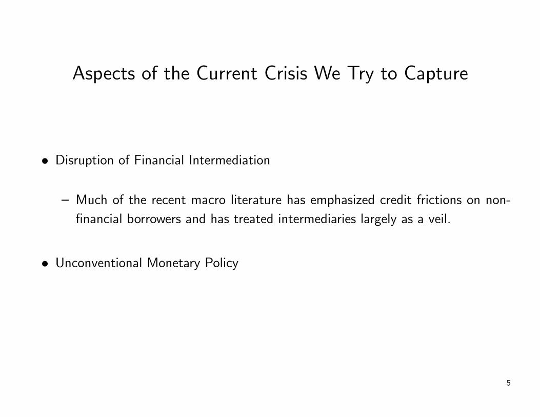
Aspects of the Current Crisis We Try to Capture
• Disruption of Financial Intermediation
— Much of the recent macro literature has emphasized credit frictions on non-financial borrowers and has treated intermediaries largely as a veil.
• Unconventional Monetary Policy
5
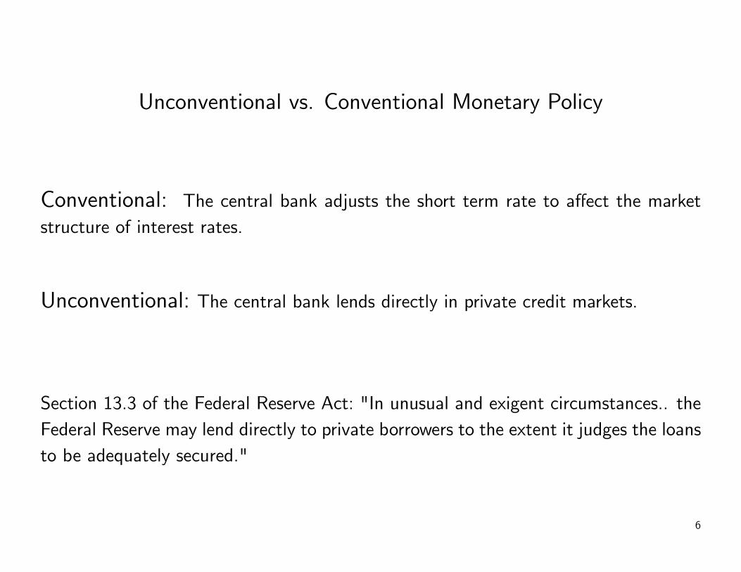
Unconventional vs. Conventional Monetary Policy
Conventional: The central bank adjusts the short term rate to affect the marketstructure of interest rates.
Unconventional: The central bank lends directly in private credit markets.
Section 13.3 of the Federal Reserve Act: "In unusual and exigent circumstances.. theFederal Reserve may lend directly to private borrowers to the extent it judges the loansto be adequately secured."
6
0
0.5
1
1.5
2
2.5
3
Aug-07 Oct-07 Dec-07 Feb-08 Apr-08 Jun-08 Aug-08 Oct-08 Dec-08 Feb-09 Apr-090
0.5
1
1.5
2
2.5
3
0
0.5
1
1.5
2
2.5
Aug-07 Oct-07 Dec-07 Feb-08 Apr-08 Jun-08 Aug-08 Oct-08 Dec-08 Feb-09 Apr-090
0.5
1
1.5
2
2.5Treasury, SFA
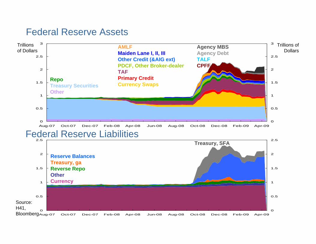
Agency MBS Agency Debt TALF CPFF
Federal Reserve Assets
Federal Reserve Liabilities
Trillions of Dollars
Trillions of Dollars
Source: H41, Bloomberg
RepoTreasury Securities Other
AMLF Maiden Lane I, II, III Other Credit (&AIG ext) PDCF, Other Broker-dealer TAF Primary Credit Currency Swaps
Reserve BalancesTreasury, gaReverse RepoOtherCurrency
Liquidity Facilities
0
100
200
300
400
500
1,400
1,500
1,600
1,700
1,800
1,900
Mar-08 Jun-08 Sep-08 Dec-08 Mar-09
CPFF and Commercial Paper OutstandingBillions of Dollars
Source: Federal Reserve Board, Haver, FDIC
Total(left axis)
Billions of Dollars
Apr 17: 1473.7
Apr 17: 235.8
Federal ReserveNet Holdings(right axis)
FDICTLGP
(right axis)
Mar 31: 336.3
-100
0
100
200
300
400
500
600
700
-100
0
100
200
300
400
500
600
Mar-08 Jun-08 Sep-08 Dec-08 Mar-09
3-month CP Rates over OIS sis oints
Source: Federal Reserve Board, Haver, Bloomberg
AA Non-Financial
Basis Points
Apr 17: 6.0
Apr 17: 61.0
AA Financial
AA Asset-Backed
Apr 17: 27.0
A2/P2/F2 Non-Financial
Apr 17: 143.0
ABCP CPFF Fee
Unsecured CPFF Fee
700Ba P
0
50
100
150
0
50
100
150
Mar-08 Jun-08 Sep-08 Dec-08 Mar-09
TSLF Schedule 1 & 2 Total OutstandingBillions of Dollars
Source: Federal Reserve Board
Schedule 2
Billions of Dollars
Apr 15: 20.6
Apr 16: 0.0
Schedule 1
-50
0
50
100
150
200
250
-50
0
50
100
150
200
250
Mar-08 Jun-08 Sep-08 Dec-08 Mar-09
Overnight Financing SpreadsBasis Points
Source: Bloomberg
Basis Points
Apr 17: 8.0
Agency MBSAgency Debt
Apr 17: 0.0
Note: Spreads are between overnight agency debt andMBS and Treasury general collateral repo rates
0
100
200
300
0
100
200
300
Mar-08 Jun-08 Sep-08 Dec-08 Mar-09
Agency MBS TransactionsBillions of Dollars
Source: Federal Reserve Board, Haver
Temporary OMOAccepted
Billions of Dollars
Apr 17: 0.0
Apr 15: 287.2
OutrightPurchases
100
150
200
250
150
200
250
300
Mar-08 Jun-08 Sep-08 Dec-08 Mar-09
Agency MBS to Average 5y and 10y YieldsBasis Points
Source: FRB, Haver, Bloomberg
Basis Points
Apr 17: 176.4
Fannie Mae
Note: Spreads are agency 30 year on-the-run coupon to average of 5 and 10 year yields
What We Do
• Develop a quantitative DSGE model that allows for financial intermediaries thatface endogenous balance sheet constraints.
• Use the model to simulate a crisis that has some of the features of the currentdownturn.
• Assess how unconventional monetary policy (direct central bank intermediation.)could moderate the downturn.
• Discuss Open Issues and Extensions
7
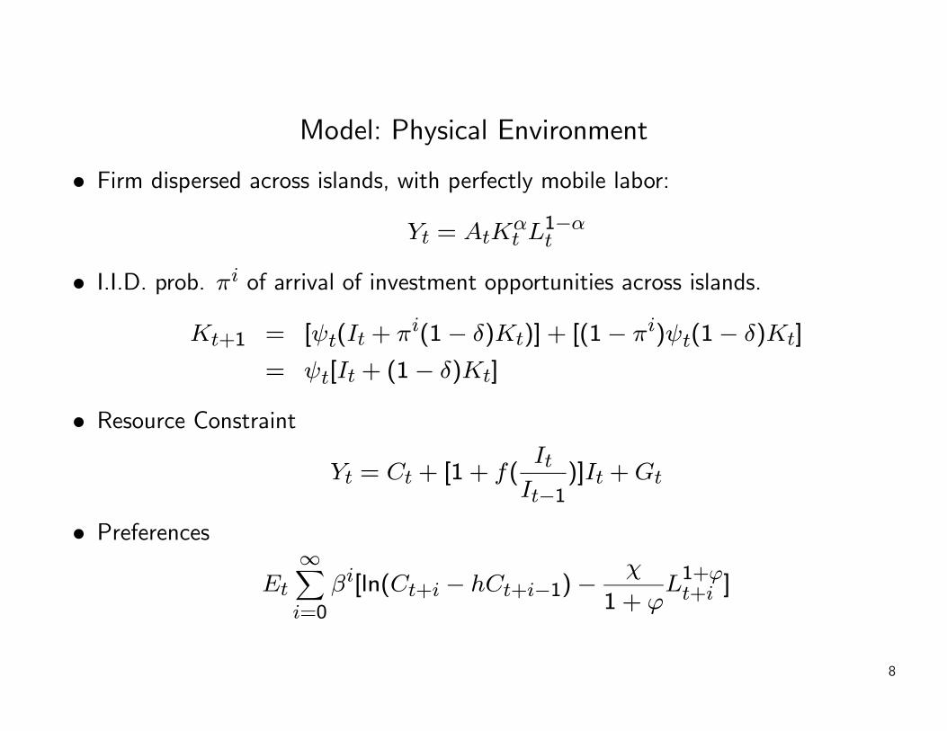
Model: Physical Environment
• Firm dispersed across islands, with perfectly mobile labor:
Yt = AtKαt L
1−αt
• I.I.D. prob. πi of arrival of investment opportunities across islands.
Kt+1 = [ψt(It + πi(1− δ)Kt)] + [(1− πi)ψt(1− δ)Kt]
= ψt[It + (1− δ)Kt]
• Resource Constraint
Yt = Ct + [1 + f(It
It−1)]It +Gt
• Preferences
Et
∞Xi=0
βi[ln(Ct+i − hCt+i−1)−χ
1 + ϕL1+ϕt+i ]
8
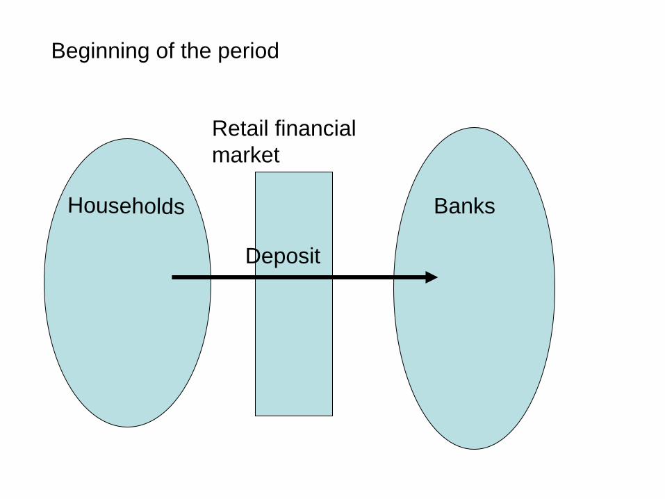
Households
Retail financial market
Banks
Deposit
Beginning of the period
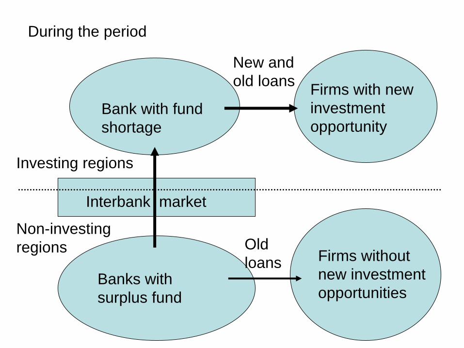
Bank with fund shortage
Interbank market
Banks with surplus fund
Firms with new investment opportunity
Firms without new investment opportunities
Old loans
New and old loans
Investing regions
Non-investing regions
During the period

Households
• Within each household, 1− f "workers" and f "bankers".
• Workers supply labor and return their wages to the household.
• Each banker manages a financial intermediary and also transfers earnings back tohousehold..
• Perfect consumption insurance within the family.
9
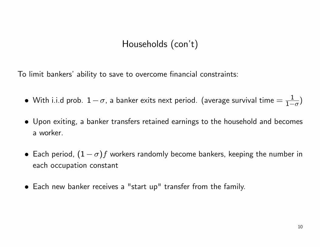
Households (con’t)
To limit bankers’ ability to save to overcome financial constraints:
• With i.i.d prob. 1−σ, a banker exits next period. (average survival time = 11−σ)
• Upon exiting, a banker transfers retained earnings to the household and becomesa worker.
• Each period, (1−σ)f workers randomly become bankers, keeping the number ineach occupation constant
• Each new banker receives a "start up" transfer from the family.
10
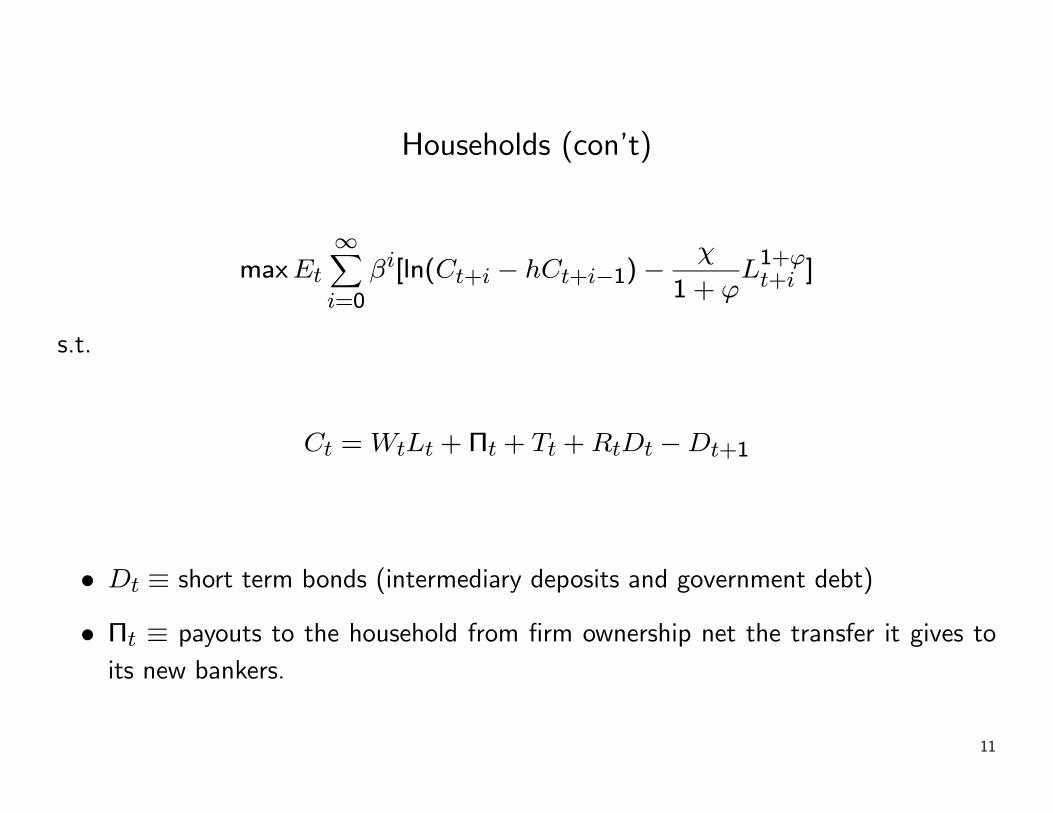
Households (con’t)
maxEt
∞Xi=0
βi[ln(Ct+i − hCt+i−1)−χ
1 + ϕL1+ϕt+i ]
s.t.
Ct =WtLt + Πt + Tt +RtDt −Dt+1
• Dt ≡ short term bonds (intermediary deposits and government debt)
• Πt ≡ payouts to the household from firm ownership net the transfer it gives toits new bankers.
11
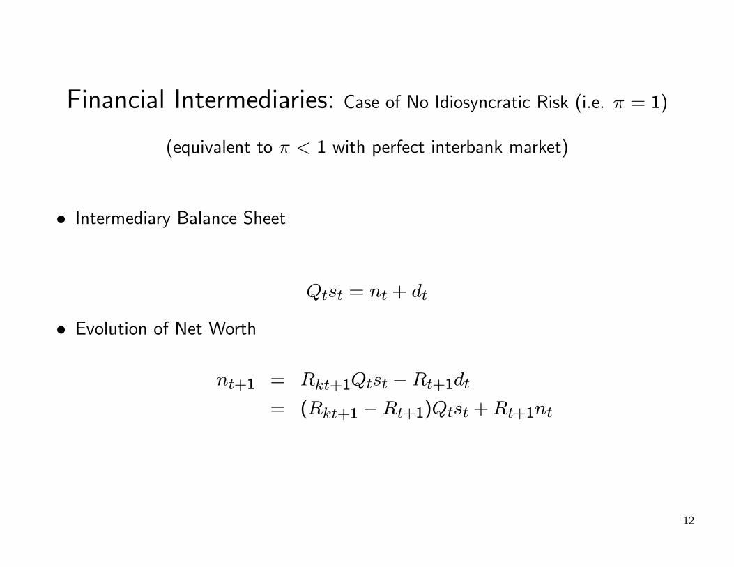
Financial Intermediaries: Case of No Idiosyncratic Risk (i.e. π = 1)
(equivalent to π < 1 with perfect interbank market)
• Intermediary Balance Sheet
Qtst = nt + dt
• Evolution of Net Worth
nt+1 = Rkt+1Qtst −Rt+1dt
= (Rkt+1 −Rt+1)Qtst +Rt+1nt
12
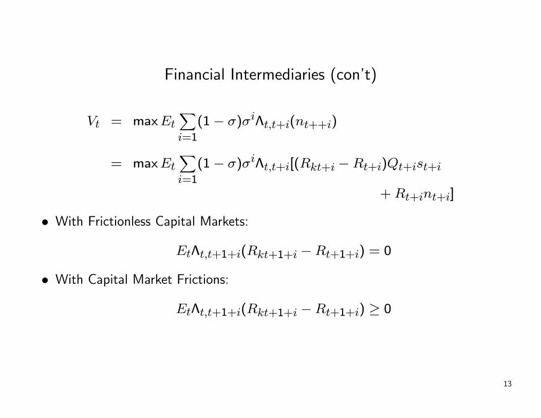
Financial Intermediaries (con’t)
Vt = maxEtXi=1
(1− σ)σiΛt,t+i(nt++i)
= maxEtXi=1
(1− σ)σiΛt,t+i[(Rkt+i −Rt+i)Qt+ist+i
+Rt+int+i]
• With Frictionless Capital Markets:
EtΛt,t+1+i(Rkt+1+i −Rt+1+i) = 0
• With Capital Market Frictions:
EtΛt,t+1+i(Rkt+1+i −Rt+1+i) ≥ 0
13
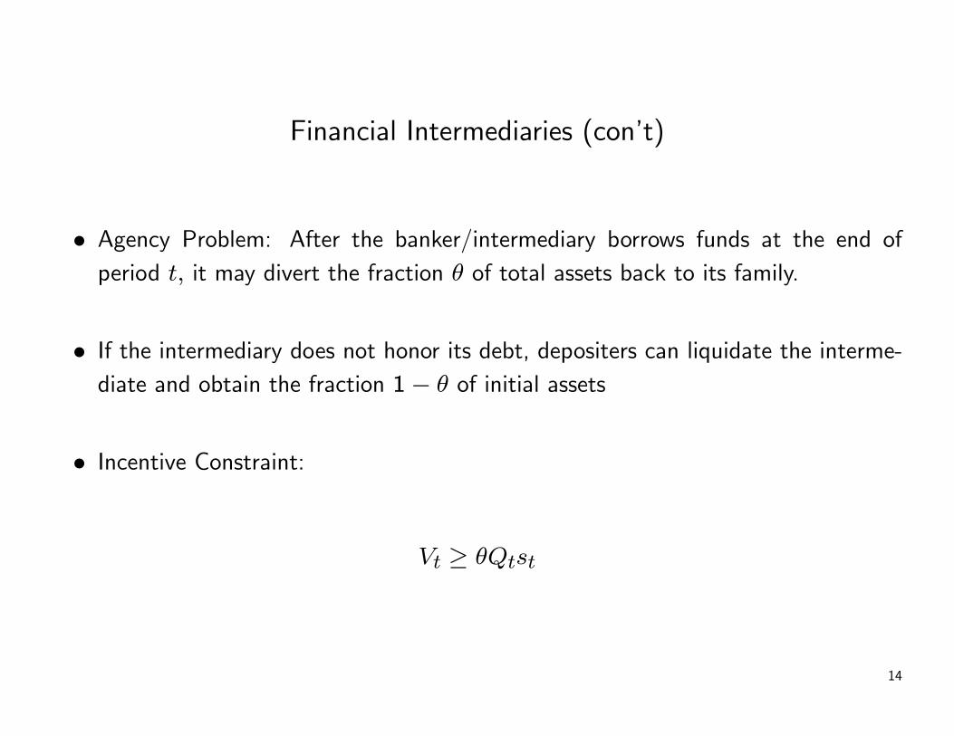
Financial Intermediaries (con’t)
• Agency Problem: After the banker/intermediary borrows funds at the end ofperiod t, it may divert the fraction θ of total assets back to its family.
• If the intermediary does not honor its debt, depositers can liquidate the interme-diate and obtain the fraction 1− θ of initial assets
• Incentive Constraint:
Vt ≥ θQtst
14
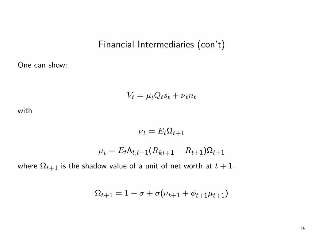
Financial Intermediaries (con’t)
One can show:
Vt = μtQtst + νtnt
with
νt = EtΩt+1
μt = EtΛt,t+1(Rkt+1 −Rt+1)Ωt+1
where Ωt+1 is the shadow value of a unit of net worth at t+ 1.
Ωt+1 = 1− σ + σ(νt+1 + φt+1μt+1)
15
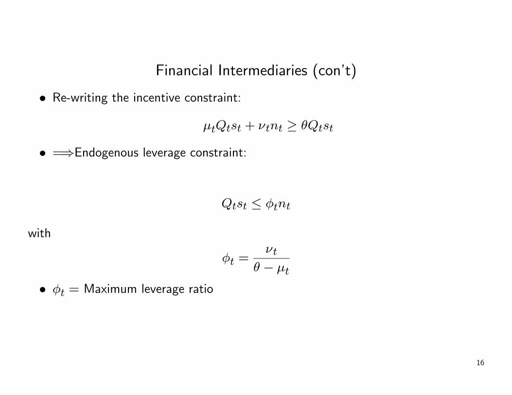
Financial Intermediaries (con’t)
• Re-writing the incentive constraint:
μtQtst + νtnt ≥ θQtst
• =⇒Endogenous leverage constraint:
Qtst ≤ φtnt
with
φt =νt
θ − μt
• φt = Maximum leverage ratio
16
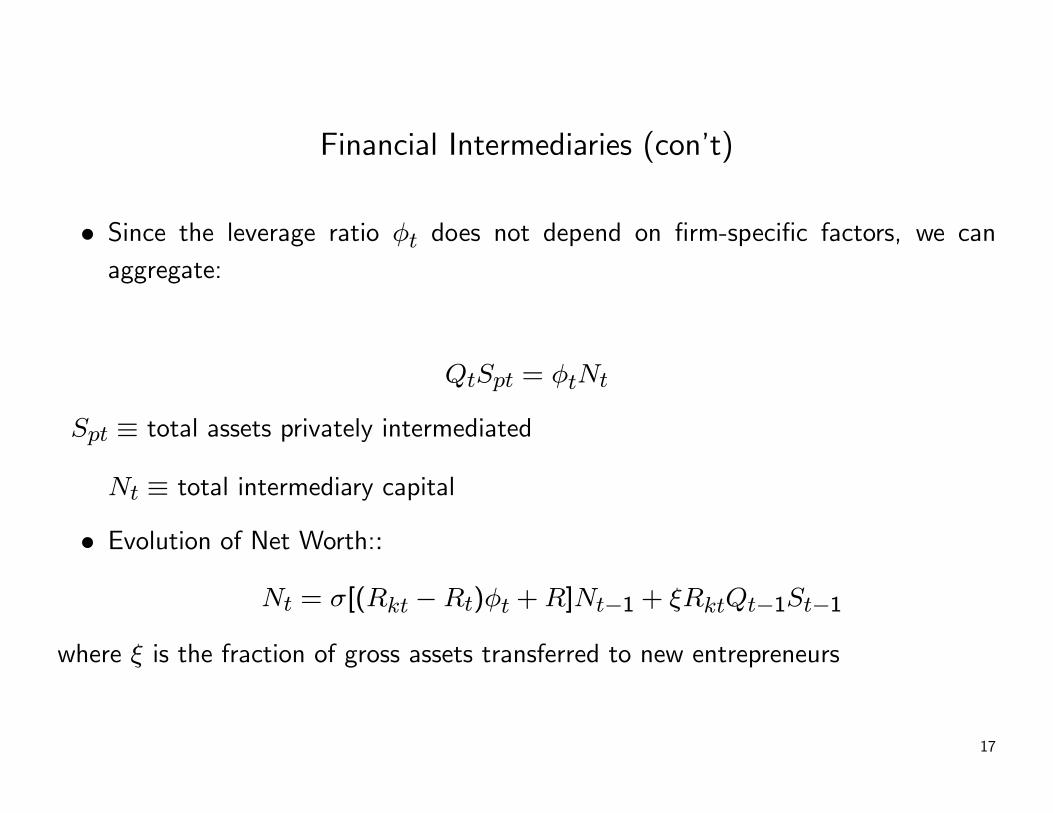
Financial Intermediaries (con’t)
• Since the leverage ratio φt does not depend on firm-specific factors, we canaggregate:
QtSpt = φtNt
Spt ≡ total assets privately intermediated
Nt ≡ total intermediary capital
• Evolution of Net Worth::
Nt = σ[(Rkt −Rt)φt +R]Nt−1 + ξRktQt−1St−1
where ξ is the fraction of gross assets transferred to new entrepreneurs
17
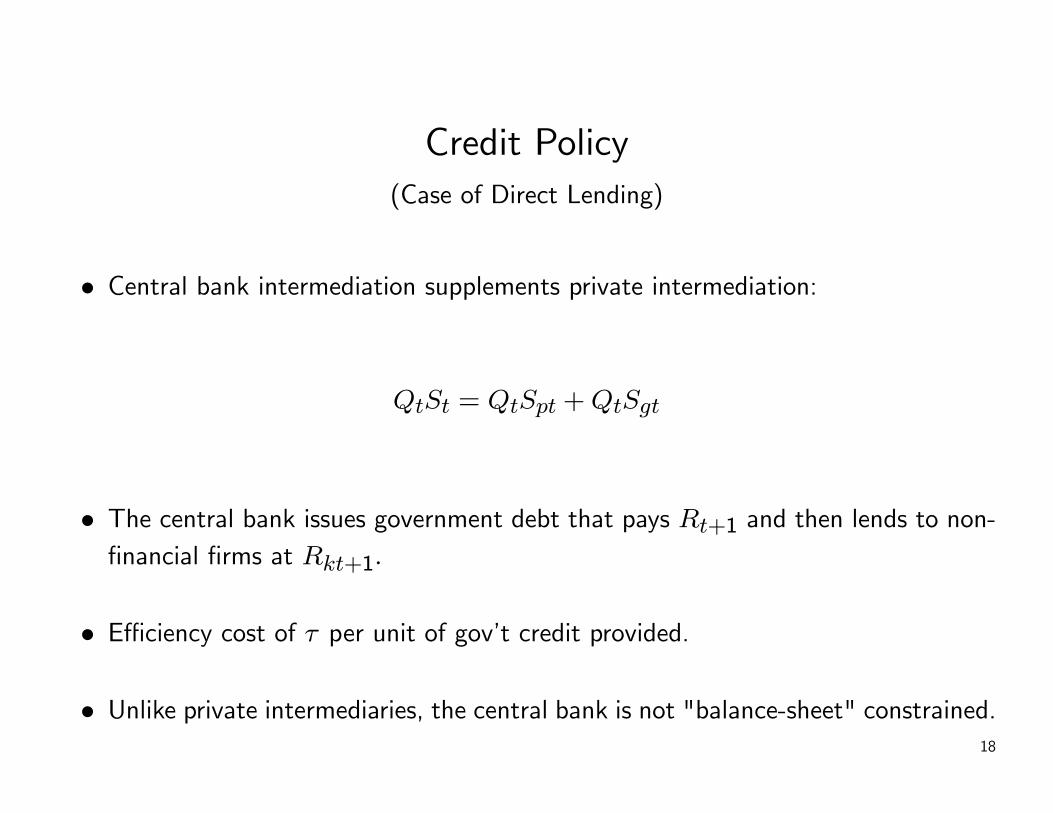
Credit Policy(Case of Direct Lending)
• Central bank intermediation supplements private intermediation:
QtSt = QtSpt +QtSgt
• The central bank issues government debt that pays Rt+1 and then lends to non-financial firms at Rkt+1.
• Efficiency cost of τ per unit of gov’t credit provided.
• Unlike private intermediaries, the central bank is not "balance-sheet" constrained.18
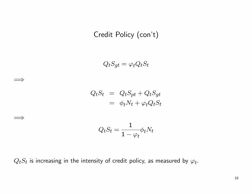
Credit Policy (con’t)
QtSgt = ϕtQtSt
=⇒
QtSt = QtSpt +QtSgt
= φtNt + ϕtQtSt
=⇒
QtSt =1
1− ϕtφtNt
QtSt is increasing in the intensity of credit policy, as measured by ϕt.
19
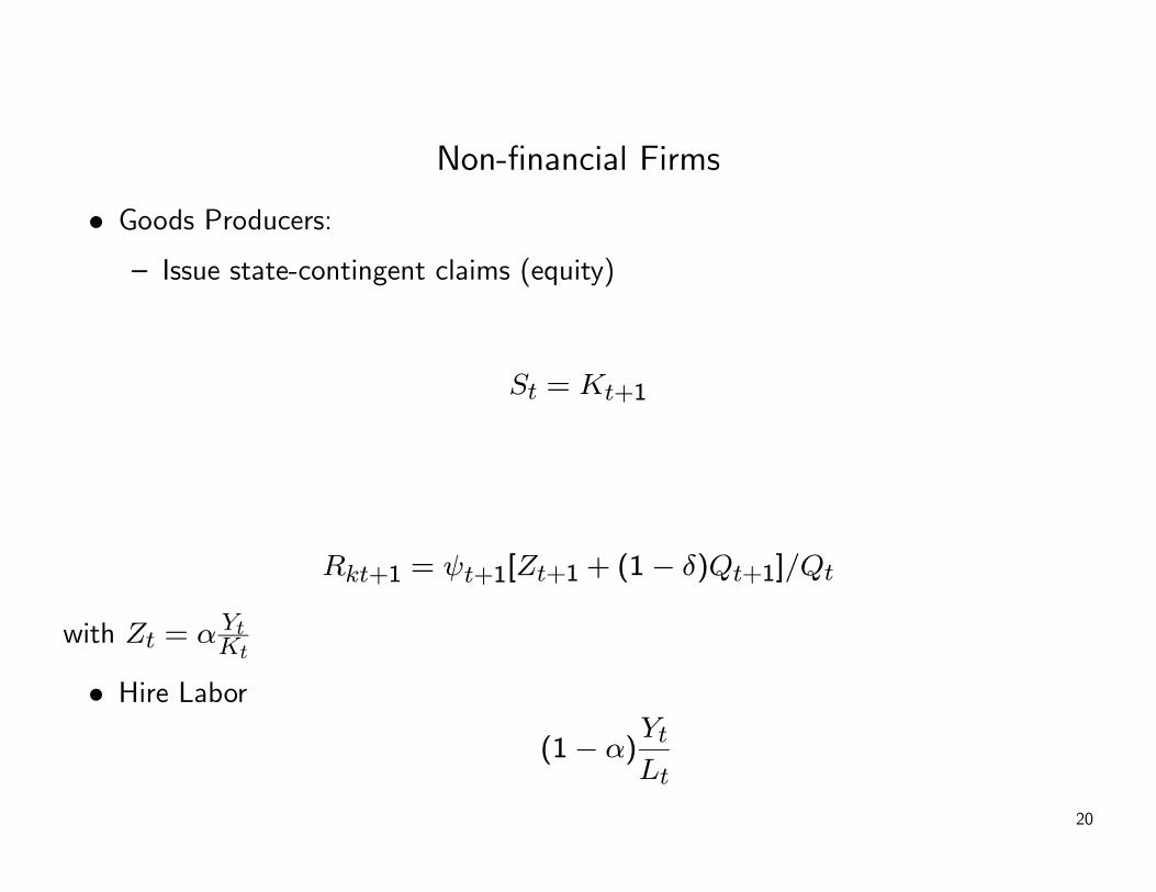
Non-financial Firms
• Goods Producers:— Issue state-contingent claims (equity)
St = Kt+1
Rkt+1 = ψt+1[Zt+1 + (1− δ)Qt+1]/Qt
with Zt = αYtKt
• Hire Labor
(1− α)Yt
Lt
20
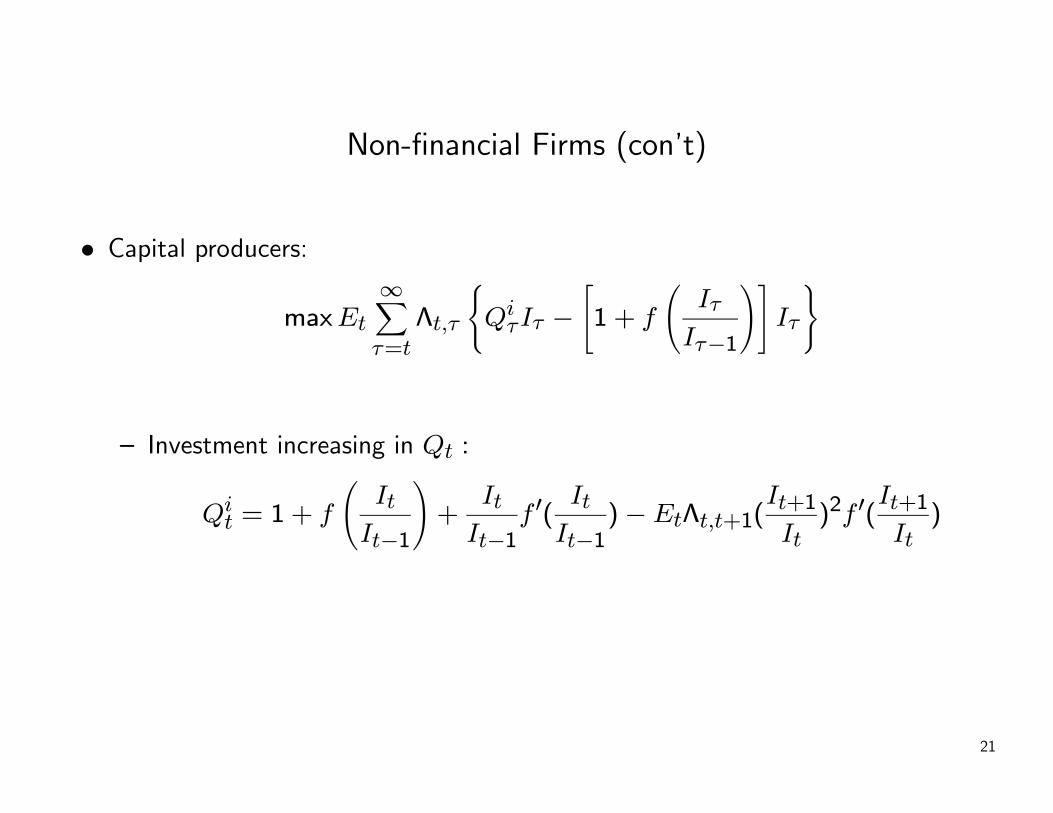
Non-financial Firms (con’t)
• Capital producers:
maxEt
∞Xτ=t
Λt,τ
(QiτIτ −
"1 + f
ÃIτ
Iτ−1
!#Iτ
)
— Investment increasing in Qt :
Qit = 1 + f
ÃIt
It−1
!+
It
It−1f 0(
It
It−1)−EtΛt,t+1(
It+1It)2f 0(
It+1It)
21
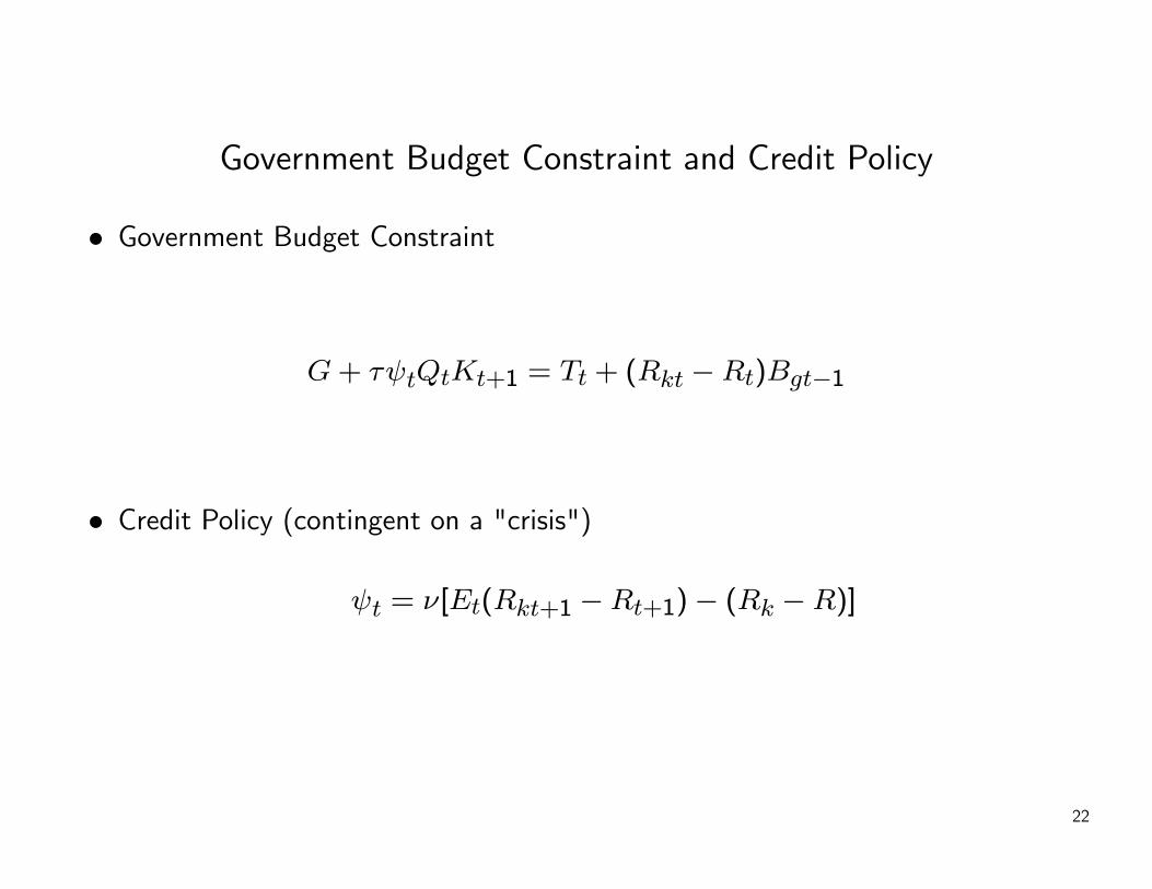
Government Budget Constraint and Credit Policy
• Government Budget Constraint
G+ τψtQtKt+1 = Tt + (Rkt −Rt)Bgt−1
• Credit Policy (contingent on a "crisis")
ψt = ν[Et(Rkt+1 −Rt+1)− (Rk −R)]
22

Table 1: Parameter Values for Baseline ModelHouseholds
β 0.990 Discount rateγ 0.500 Habit parameterχ 5.584 Relative utility weight of laborϕ 0.333 Inverse Frisch elasticity of labor supply
Financial Intermediariesπi 0.250 Probability of new investment opportunitiesθ 0.383 Fraction of assets divertable: Perfect interbank market
0.129 Fraction of assets divertable: Imperfect interbank marketξ 0.003 Transfer to entering bankers: Perfect interbank market
0.002 Transfer to entering bankers: Imperfect interbank marketσ 0.972 Survival rate of the bankers
Intermediate good firmsα 0.330 Effective capital shareδ 0.025 Steady state depreciation rate
Capital Producing FirmsIf”/f 0 1.000 Inverse elasticity of net investment to the price of capital
GovernmentGY
0.200 Steady state proportion of government expenditures
41
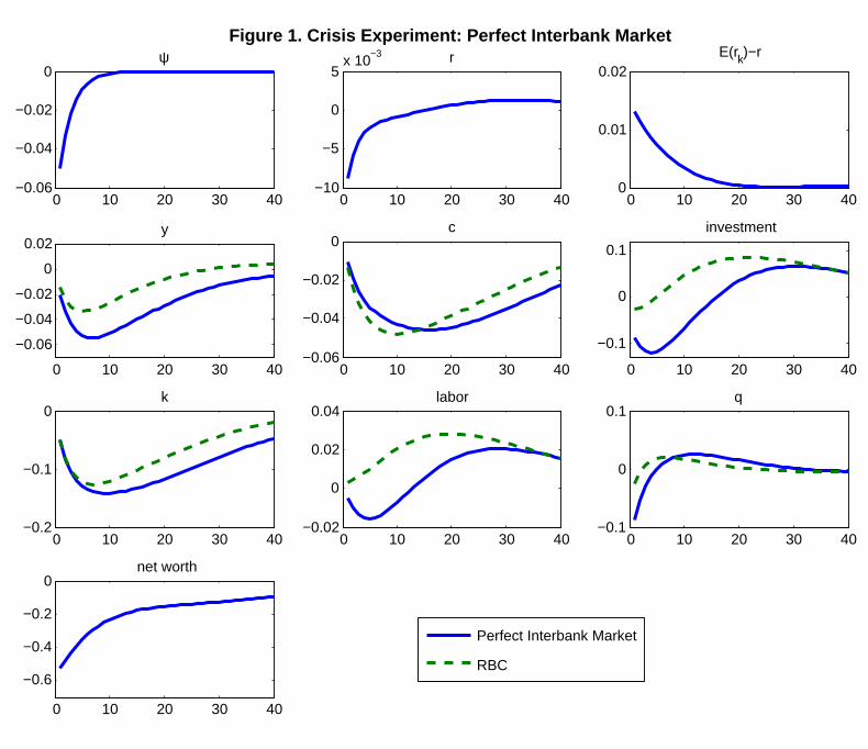
0 10 20 30 40−0.06
−0.04
−0.02
0ψ
0 10 20 30 40−10
−5
0
5x 10
−3 r
0 10 20 30 400
0.01
0.02E(rk)−r
0 10 20 30 40
−0.06
−0.04
−0.02
0
0.02y
0 10 20 30 40−0.06
−0.04
−0.02
0c
0 10 20 30 40
−0.1
0
0.1
investment
0 10 20 30 40−0.2
−0.1
0k
0 10 20 30 40−0.02
0
0.02
0.04labor
0 10 20 30 40−0.1
0
0.1q
0 10 20 30 40
−0.6
−0.4
−0.2
0net worth
Perfect Interbank Market
RBC
Figure 1. Crisis Experiment: Perfect Interbank Market
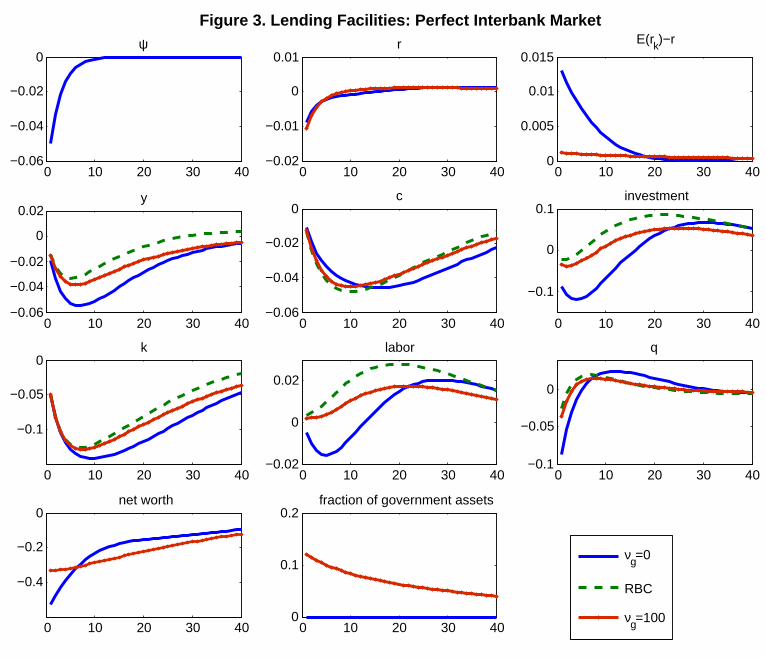
0 10 20 30 40−0.06
−0.04
−0.02
0ψ
0 10 20 30 40−0.02
−0.01
0
0.01r
0 10 20 30 400
0.005
0.01
0.015E(rk)−r
0 10 20 30 40−0.06
−0.04
−0.02
0
0.02y
0 10 20 30 40−0.06
−0.04
−0.02
0c
0 10 20 30 40
−0.1
0
0.1investment
0 10 20 30 40
−0.1
−0.05
0k
0 10 20 30 40−0.02
0
0.02
labor
0 10 20 30 40−0.1
−0.05
0
q
0 10 20 30 40
−0.4
−0.2
0net worth
0 10 20 30 400
0.1
0.2fraction of government assets
νg=0
RBC
νg=100
Figure 3. Lending Facilities: Perfect Interbank Market
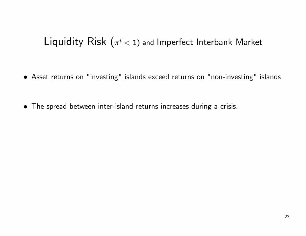
Liquidity Risk (πi < 1) and Imperfect Interbank Market
• Asset returns on "investing" islands exceed returns on "non-investing" islands
• The spread between inter-island returns increases during a crisis.
23
Liquidity Risk (πi < 1), con’t
• for h = i, n
Qht s
ht = nht + bht + dt.
where bht is interbank borrowing
• net worth:
nht = [Zt + (1− δ)Qht ]ψtQ
h−1t−1st−1 −Rbtb
ht−1 −Rtdt−1,
Rh−1hkt =
[Zt + (1− δ)Qht ]ψt
Qh−1t−1
24
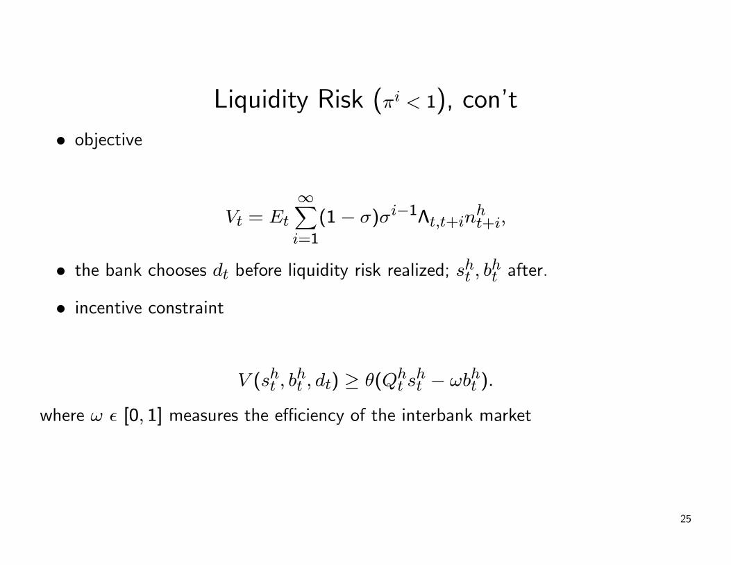
Liquidity Risk (πi < 1), con’t• objective
Vt = Et
∞Xi=1
(1− σ)σi−1Λt,t+inht+i,
• the bank chooses dt before liquidity risk realized; sht , bht after.
• incentive constraint
V (sht , bht , dt) ≥ θ(Qh
t sht − ωbht ).
where ω [0, 1] measures the efficiency of the interbank market
25
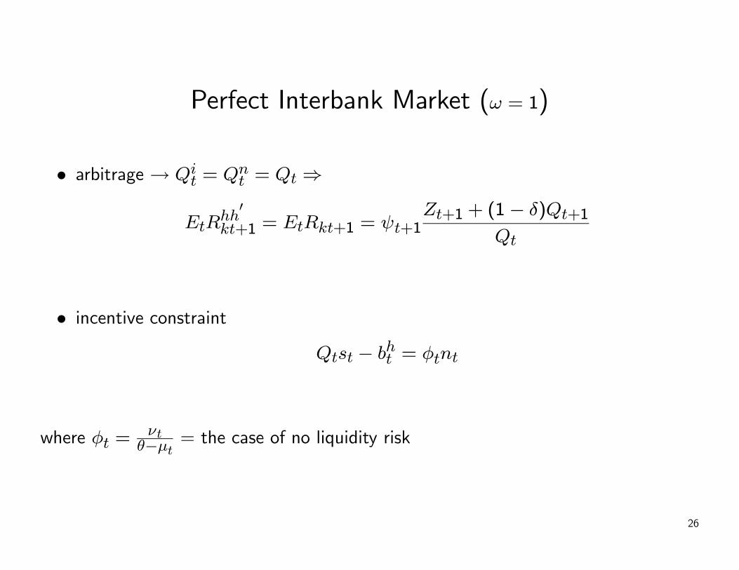
Perfect Interbank Market (ω = 1)
• arbitrage → Qit = Qn
t = Qt⇒
EtRhh0
kt+1 = EtRkt+1 = ψt+1Zt+1 + (1− δ)Qt+1
Qt
• incentive constraint
Qtst − bht = φtnt
where φt =νt
θ−μt = the case of no liquidity risk
26
Perfect Interbank Market (ω = 1)
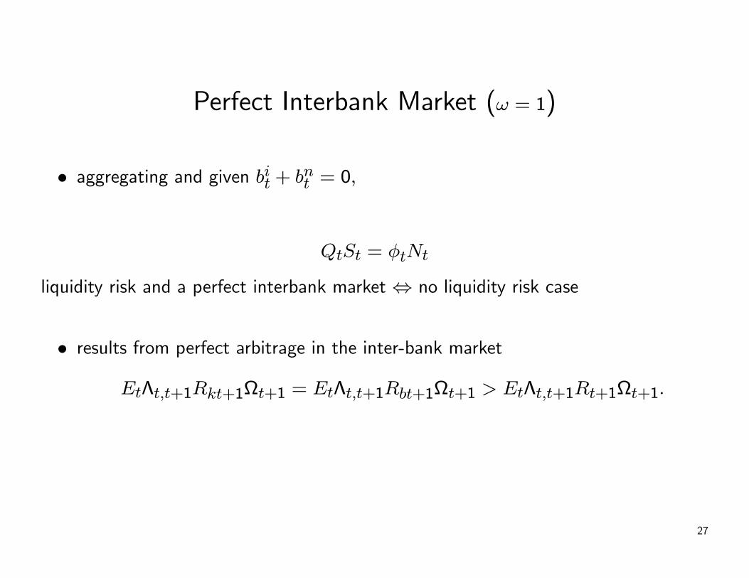
• aggregating and given bit + bnt = 0,
QtSt = φtNt
liquidity risk and a perfect interbank market ⇔ no liquidity risk case
• results from perfect arbitrage in the inter-bank market
EtΛt,t+1Rkt+1Ωt+1 = EtΛt,t+1Rbt+1Ωt+1 > EtΛt,t+1Rt+1Ωt+1.
27
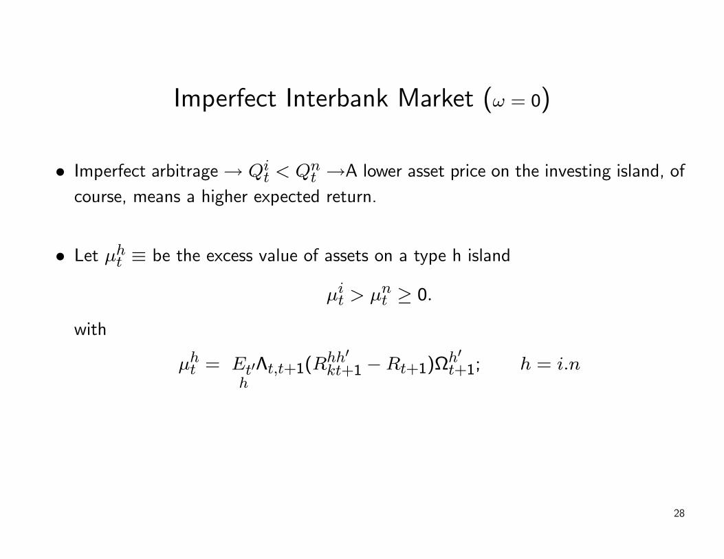
Imperfect Interbank Market (ω = 0)
• Imperfect arbitrage→ Qit < Qn
t →A lower asset price on the investing island, ofcourse, means a higher expected return.
• Let μht ≡ be the excess value of assets on a type h island
μit > μnt ≥ 0.
with
μht = Et0hΛt,t+1(R
hh0kt+1 −Rt+1)Ω
h0t+1; h = i.n
28
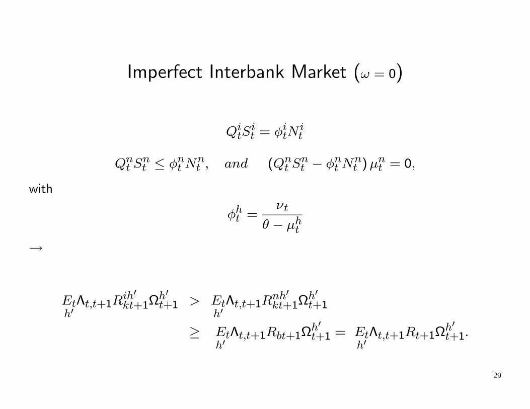
Imperfect Interbank Market (ω = 0)
QitS
it = φitN
it
Qnt S
nt ≤ φnt N
nt , and (Qn
t Snt − φnt N
nt )μ
nt = 0,
with
φht =νt
θ − μht
→
Eth0Λt,t+1R
ih0kt+1Ω
h0t+1 > Et
h0Λt,t+1R
nh0kt+1Ω
h0t+1
≥ Eth0
Λt,t+1Rbt+1Ωh0t+1 = Et
h0Λt,t+1Rt+1Ω
h0t+1.
29
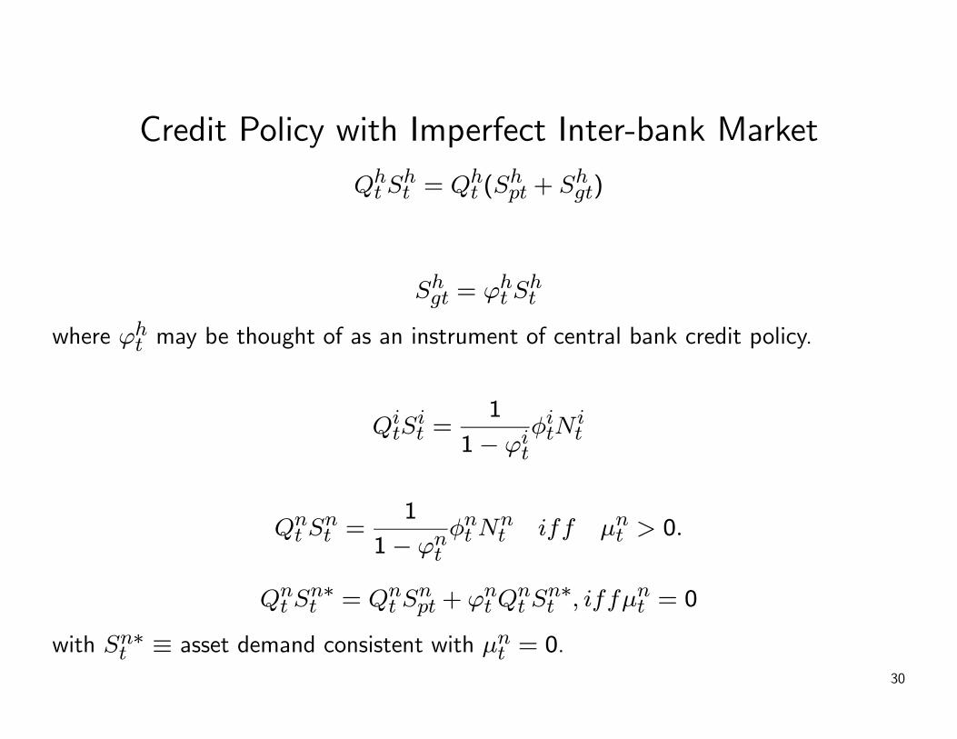
Credit Policy with Imperfect Inter-bank Market
Qht S
ht = Qh
t (Shpt + Shgt)
Shgt = ϕht Sht
where ϕht may be thought of as an instrument of central bank credit policy.
QitS
it =
1
1− ϕitφitN
it
Qnt S
nt =
1
1− ϕntφnt N
nt iff μnt > 0.
Qnt S
n∗t = Qn
t Snpt + ϕnt Q
nt S
n∗t , iffμnt = 0
with Sn∗t ≡ asset demand consistent with μnt = 0.30
0 10 20 30 40−0.06
−0.04
−0.02
0ψ
0 10 20 30 40−10
−5
0
5x 10
−3 r
0 10 20 30 400
0.02
0.04
0.06spread
0 10 20 30 40
−0.06
−0.04
−0.02
0
0.02y
0 10 20 30 40−0.06
−0.04
−0.02
0c
0 10 20 30 40−0.2
−0.1
0
0.1investment
0 10 20 30 40
−0.15
−0.1
−0.05
0k
0 10 20 30 40
−0.02
0
0.02
labor
0 10 20 30 40
−0.1
−0.05
0
0.05q
0 10 20 30 40
−0.6
−0.4
−0.2
0net worth
Imperfect Interbank Market (πi=0.25)
RBC
Perfect Interbank Market
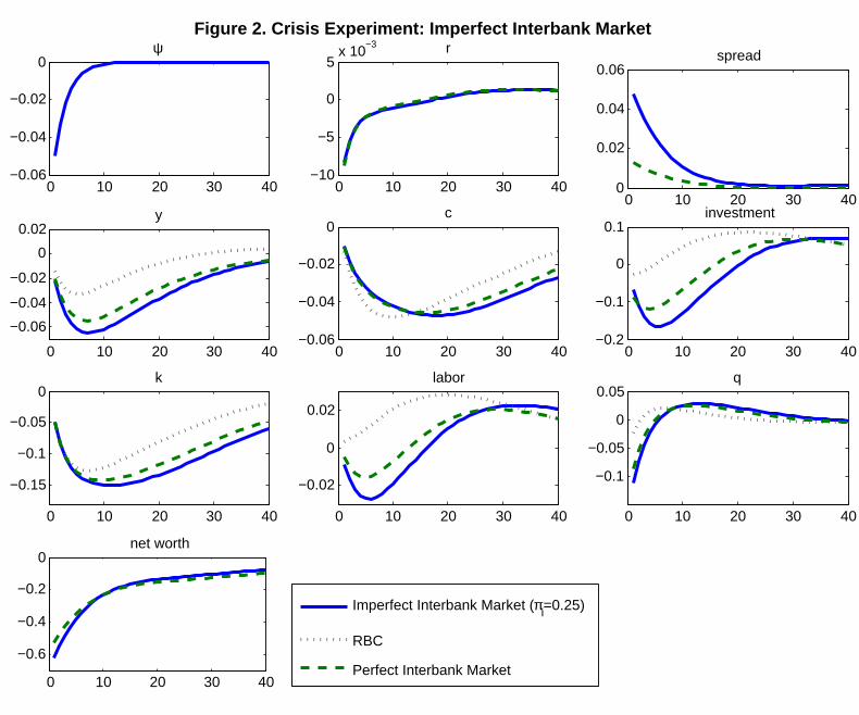
Figure 2. Crisis Experiment: Imperfect Interbank Market
0 10 20 30 40−0.06
−0.04
−0.02
0ψ
0 10 20 30 40−0.02
−0.01
0
0.01r
0 10 20 30 400
0.02
0.04
0.06spread
0 10 20 30 40
−0.06
−0.04
−0.02
0
y
0 10 20 30 40−0.06
−0.04
−0.02
0c
0 10 20 30 40−0.2
−0.1
0
0.1investment
0 10 20 30 40−0.2
−0.1
0k
0 10 20 30 40
−0.02
0
0.02
labor
0 10 20 30 40
−0.1
−0.05
0
0.05q
0 10 20 30 40−0.8
−0.6
−0.4
−0.2
net worth
0 10 20 30 400
0.02
0.04
0.06
fraction of government assets
νg=0
RBC
νg=100
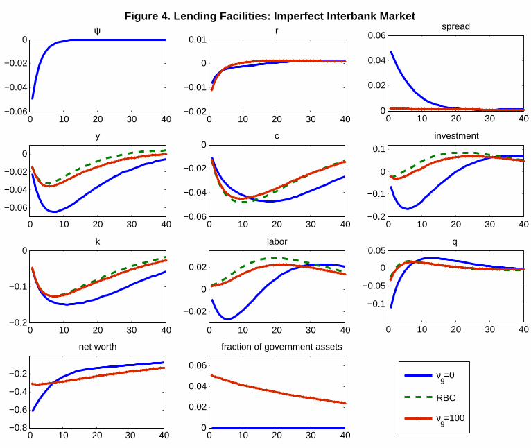
Figure 4. Lending Facilities: Imperfect Interbank Market
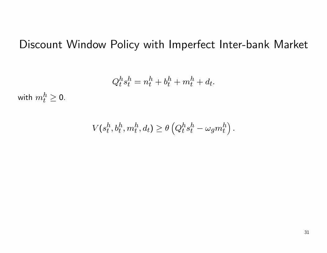
Discount Window Policy with Imperfect Inter-bank Market
Qht s
ht = nht + bht +mh
t + dt.
with mht ≥ 0.
V (sht , bht ,m
ht , dt) ≥ θ
³Qht s
ht − ωgm
ht
´.
31
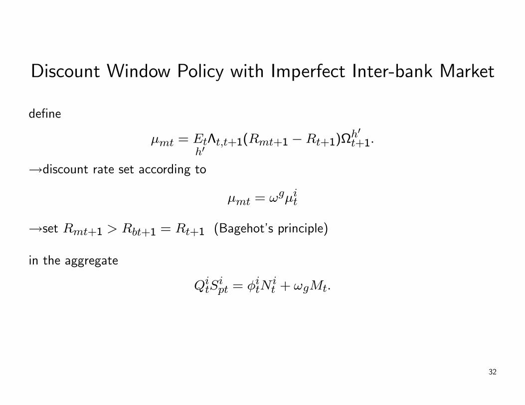
Discount Window Policy with Imperfect Inter-bank Market
define
μmt = Eth0Λt,t+1(Rmt+1 −Rt+1)Ω
h0t+1.
→discount rate set according to
μmt = ωgμit
→set Rmt+1 > Rbt+1 = Rt+1 (Bagehot’s principle)
in the aggregate
QitS
ipt = φitN
it + ωgMt.
32
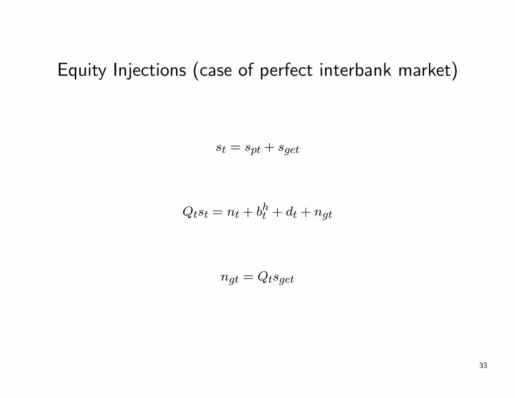
Equity Injections (case of perfect interbank market)
st = spt + sget
Qtst = nt + bht + dt + ngt
ngt = Qtsget
33
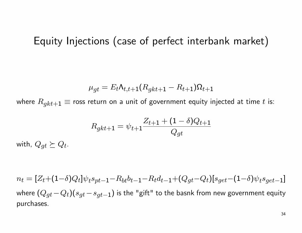
Equity Injections (case of perfect interbank market)
μgt = EtΛt,t+1(Rgkt+1 −Rt+1)Ωt+1
where Rgkt+1 ≡ ross return on a unit of government equity injected at time t is:
Rgkt+1 = ψt+1Zt+1 + (1− δ)Qt+1
Qgt
with, Qgt º Qt.
nt = [Zt+(1−δ)Qt]ψtspt−1−Rbtbt−1−Rtdt−1+(Qgt−Qt)[sget−(1−δ)ψtsget−1]
where (Qgt−Qt)(sgt−sgt−1) is the "gift" to the basnk from new government equitypurchases.
34
Equity Injections (case of perfect interbank market)
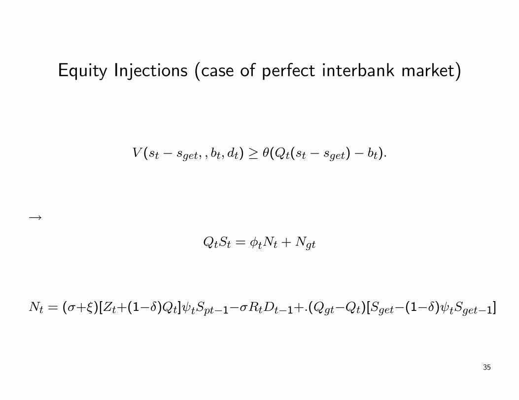
V (st − sget, , bt, dt) ≥ θ(Qt(st − sget)− bt).
→
QtSt = φtNt +Ngt
Nt = (σ+ξ)[Zt+(1−δ)Qt]ψtSpt−1−σRtDt−1+.(Qgt−Qt)[Sget−(1−δ)ψtSget−1]
35

.Issues
1. Idiosyncratic Asset Risk and Default
2. Illiquidity and Market Thinness
3. Maturity Structure
4. Bank Equity
5. Capital Requirements and Regulation,
and so on....
36