financial markets group - lse research onlineeprints.lse.ac.uk/24909/1/dp405.pdf · financial...

_______________________________________________

FINANCIAL MARKETS GROUP AN ESRC RESEARCH CENTRE

_______________________________________________

LONDON SCHOOL OF ECONOMICS

Any opinions expressed are those of the author and not necessarily those of the Financial Markets Group.

ISSN 0956-8549-405

Momentum in the UK Stock Market

By

Mark T Hon

and Ian Tonks

DISCUSSION PAPER 405

February 2002


By

Mark T. Hon [email protected]

and

Ian Tonks1

[email protected]

December 2001

Department of Economics, University of Bristol, 8 Woodland Road, Bristol BS8 1TN, United Kingdom,

Tel: +44 (0)117-928-8435,

Fax: +44 (0)117-928-8577,

1 We are grateful for comments from David Ashton and Richard Harris. Errors remain our own responsibility

2


Abstract

This paper investigates the presence of abnormal returns through the use of trading strategies that exploit the predictability of short run stock price movements. Based on historical returns of the largest set of individual securities in the UK stock market examined to date, this paper identifies profitable momentum trading strategies as investment tools over the period 1955-96. Our results show that returns on trading strategies cannot be accounted for by a simple adjustment for beta-risk. Also, although we find some evidence of a size effect in the UK stock market, this phenomenon cannot explain the momentum profits. The paper finds that these profitable investment strategies are apparent in the sub-sample 1977-96, in line with Liu, Strong and Xu (1999). However, they are not present in the earlier 1955-76 period. The implication is that momentum is not a general feature of the UK stock market, but is only apparent over certain time periods.

JEL Classification: G14 Keywords: Momentum, Contrarian strategies

3

1. Introduction

Recently there has been much work on the profitability of trading strategies in stock

markets. This work stands in stark contrast to the previously well-accepted doctrine of the

efficient markets hypothesis. Under the null hypothesis of weak-form market efficiency, the

performance of portfolios of stocks should be independent of past returns. However

empirical research has shown that asset returns tend to exhibit some form of positive

autocorrelation in the short to medium term; but mean-revert over longer horizons. There are

two prevalent types of trading methodologies used to take advantage of serial correlation in

stock price returns: momentum trading and contrarian strategies. Momentum strategies are

at one end of the spectrum, and rely on short-run positive autocorrelation in returns. They

generate abnormal profits by following a rule of buying past winners and selling past losers.

Liu et al (1999) reports on the profitability of momentum strategies in the UK over the

period 1977-96. In contrast contrarian strategies are based on negative serial correlation in

stock prices such that selling winners and buying losers generates abnormal profits.

The current paper assesses the profitability of momentum strategies on the UK stock

market using the most comprehensive set of data available to date. This is important since

any rejection of the efficient markets hypothesis may be a consequence of a short span of

data, and raises the question as to whether the documented rejection of the efficient markets

hypothesis is a property of the sample or whether it is a genuine empirical regularity. In fact

Liu et al (1999) argue that their momentum results are robust across two sub-samples in

their dataset. However we find that extending the data on UK returns back to 1955, the

momentum effects apparent from 1977 onwards do not exist in the earlier period 1955-76.

The next section presents an overview of the empirical literature on serial correlation in stock

prices. Section 3 describes the methodology and dataset used in the current paper, Section

4 covers the potential problems and safeguards applied, and Section 5 presents the

empirical results. Sections 6 and 7 report on the empirical findings after controlling for risk

and size respectively, and Section 8 concludes.

2. Literature Review

In recent years, there has been a surge of articles on the predictability of asset returns based

4

on historical data. DeBondt and Thaler (1985, 1987) identified long run return reversals,

which suggest that contrarian strategies of selling past winners and buying past losers

generate abnormal returns.2 Other papers (Fama and French, 1988, Lo and MacKinlay,

1988, Porterba and Summers, 1988, and Jegadeesh, 1990) have also found evidence of

negative serial correlation in long horizon stock returns, but positive correlation at shorter

intervals.3 Positive autocorrelation at short-time intervals implies that momentum strategies

might yield profitable trading opportunities. Jegadeesh and Titman (1993, 1995) report

significant positive returns when stocks are bought and sold based on short-run historical

returns. Firms with higher returns over the past 3- to 12- months subsequently outperform

firms with lower returns over the same period. Using data from the NYSE and stocks listed

on the American Stock Exchange (AMEX) from 1965 to 1989, they rank stocks in

ascending order based on their past 3- to 12- month returns, and form ten equally weighted

deciles of stock portfolios. The top decile is classified as the ‘loser’ decile and the bottom

decile as the ‘winner’ decile. In each overlapping period, the strategy is then to buy the

winner decile and sell the loser decile with holding periods of 3- to 12- months. Grinblatt

and Titman (1989) document abnormal returns from following this trading strategy;

however, the profits generated in the first year after portfolio formation dissipates in the

following two years. Grundy and Martin (1998) use the Fama-French three factor risk-

adjusted returns model to record profitability of more than 1.3 percent per month using

momentum strategies on NYSE and AMEX stocks over the period 1966 to 1995.

Moskowitz and Grinblatt (1999) find strong momentum effect across industries: when

stocks from past winning industries were bought and stocks from past losing industries sold,

the strategy was highly profitable, even after controlling for cross-sectional dispersion in

mean returns and likely microstructure differences. Conrad and Kaul (1998) in a study on

2 For the UK Power, Lonie and Lonie (1991), MacDonald and Power (1991), and Dissanaike (1997) find that contrarian strategies based on monthly returns of UK companies yield abnormal profits. However Clare and Thomas (1995) using randomly selected UK annual returns data over the period 1955 to 1990 conclude that the documented overreaction was a manifestation of the small firm effect. 3 These findings are contentious, and a number of arguments have been suggested that would reduce the profitability from exploiting these contrarian patterns: risk (Chan, 1988, Ball and Kothari, 1989, Fama and French, 1996), size effects (Zarowin, 1990), and microstructure effects (Kaul and Nimalendran, 1990, Lo and Mackinlay, 1990).

5

NYSE and AMEX securities between the period of 1926 to 1989 report the success of

contrarian strategies at long horizons and momentum trading strategies at medium horizons.

Chan, Jegadeesh and Lakonishok (1996) found that momentum effects are distinct from

post-earnings announcement drift.

The momentum anomaly is not confined to the US. Rouwenhourst (1998) tests the

profitability of momentum strategies in international equity markets. Monthly total returns

from 12 European countries during the period 1980 to 1995 were used to form relative

strength portfolios. After correcting for risk, it was found that winner portfolios outperform

loser portfolios by more than 1 percent per month and the overall returns on all momentum

portfolios are similar to the findings of Jegadeesh and Titman (1993) for the US market.

Using monthly returns from stock indices of 16 countries for the period of 1970 to 1995,

Richards (1997) found that the momentum effect is strongest at the 6-month horizon with an

annual excess return of 3.4 percent. For horizons longer than one year, ranking period

losers began to outperform winners with an average annualised excess returns of more than

5.8 percent. Clare and Thomas (1995) and Dissanaike (1997) both find some evidence of

momentum in the UK, though the focus of their work is on long-run over-reaction, rather

than short-term momentum effects. Both studies use a sample of returns from securities on

the LSPD database. Clare and Thomas (1995) using a random sample of stocks on the

LSPD over the period 1955-1990 find weak evidence of momentum at the 12-month

horizon, in that although winners outperform losers, the average return difference is

insignificantly different from zero. They find that at the 24-month (and also at the 36-month)

horizon there is significant evidence of over-reaction. Dissanaike (1997) using a sample of

larger stocks that are constituents of the FT500 Index, over the period 1975-1991 find that

there is some evidence of momentum (rather than reversal) up to the 24-month horizon.

Hence the results at the 24-month horizon from the Clare and Thomas (1995) and

Dissanaike (1997) are contradictory. A recent paper by Liu et al (1999) which focuses on

short-run returns identifies the presence of momentum profits in UK stock returns over the

period of January 1977 to December 1996. Controlling for systematic risk, size, price,

book-to-market ratio, or cash earnings-to-price ratio did not eliminate momentum profits.

In addition they examine momentum profits in sub-samples of their dataset, and argue that

6

momentum effects are a robust feature of the UK equity market.

In summary the evidence from above studies shows that over short to medium-term

(i.e., 3- to 12- month) horizons, momentum strategies are most profitable; while contrarian

strategies prove to be more profitable over the very short-term (i.e., 1- to 4- week) and

long-term (i.e., 36- to 60- month) horizon.4

3. Methodology and Data

In this paper we test the null hypothesis of weak form stock market efficiency, by

examining whether returns are independent over short time-horizons. Portfolios are formed

on the basis of past returns, with the top batch of the ranked stocks labelled the ‘loser’

portfolio and the bottom the ‘winner’ portfolio. Momentum strategies form portfolios on the

basis of past short-run returns, by buying winner portfolios and selling loser portfolios. The

efficient market hypothesis (EMH) predicts that these winner-loser portfolios will yield zero

profits. However if asset prices exhibit mean-reversion or overreaction, the winner-loser

portfolios will generate profits over some horizons in the sample period. Our objective is to

extend the time frame used by Liu et al (1999) to examine the claim that momentum effects

are a robust feature of the UK equity market.

The test for the profitability of momentum trading strategies in the paper is based on

the methodology used by DeBondt and Thaler (1985, 1987) and Jegadeesh and Titman

(1993)5. These papers assess the profitability of JxK trading strategies, where securities are

assigned to portfolios according to a ranking in period t based on the previous J months'

returns. In month t, we form a winner-loser portfolio, where an investor goes short on the

loser portfolio and takes on a long position on the winner portfolio for the following K-

4 While most of the empirical works point to some level of predictability in stock returns, there is disagreement about the underlying explanations. Alternative theoretical models of investor behaviour by Daniel, Hirshleifer and Subrahmanyam (1998), DeLong et al. (1990), Baberis, Shleifer and Vishny (1998), Berk, Green, and Naik (1999), Hong and Stein (1999), Hong, Lim and Stein (2000) have been proposed to explain these serial correlation properties in stock prices. 5 This study will be based on log returns rather than raw returns. Conrad and Kaul (1993) and Ball et al. (1995) point out that results documented by DeBondt and Thaler (1985, 1987), Chan (1988), Ball and Kothari (1989), and Chopra et al. (1992), suffer from measurement errors as raw returns were used in estimating portfolio performance.

7

month horizon. Thus, based on J months of historical data, portfolios are held for a horizon

of K months after being executed in month t.

The data is taken from the London Share Price Database (LSPD) tape of returns of

UK companies from January 1955 to December 1996. This tape consists of all companies

quoted on the London Stock Exchange since 1975. For the period before 1975 the file is

made up of a number of different samples. As well as a random sample of 33% of the

companies quoted on the Exchange between 1955 and 1974, there are 33% of new issues

in each year 1955-74. The tape also includes the 500 largest companies by market value in

January 1955, and the 200 largest in December 1972, plus all 100 companies in the

brewing industry. There are a total of 1,571 securities in the sample starting in January 1955,

and as securities enter and leave the Exchange over the next 40 years, there are over 6,600

securities in total over the entire sample period.

Securities are selected based on their returns over the past 3 to 24 months. Holding

periods examined will also vary from 3 to 24 months. In fact there are 8 reported lags and 8

horizons used in total (i.e., 3, 6, 9, 12, 15, 18, 21, 24-month intervals for every JxK

strategy). For every stock i on the LSPD tape without any missing values between test

intervals, an equally weighted portfolio of losers and winners are formed based on

cumulative monthly returns. The procedure is repeated up to 64 times (i.e., once for each

JxK trading strategy) using non-overlapping observations starting January 1955 to

December 1996.

The trading strategy consists of three basic steps. First, individual stocks are ranked

according to Cumulative Continuous Returns (CCR) for each stock i on past J months of

continuously compounded monthly returns in the initial portfolio formation period.

??

??

?J

titi RCCR

1

where Rit is the log-return in month t for company i.

Second, in each month t, the entire series of securities at that date is divided into ten

8

equal deciles in ascending order based on CCRis. Securities are assigned in equal numbers

to each of ten portfolios. The top decile (decile 1) is designated the ‘loser’ portfolio and the

bottom decile (decile 10) ‘winner’ portfolio. In month t, we form a winner-loser portfolio

whereby an investor goes short on the loser portfolio and takes on a long position on the

winner portfolio.

The third and final step of the trading rule is to determine the profits of a winner minus

loser portfolio ( loserwinnerR ? ) where the mean monthly returns from past loser portfolios

( loserR ) are subtracted from mean monthly returns of past winner portfolios ( winnerR ):

loserwinnerR ? = winnerR - loserR

The trading strategies are replicated for each stated period and the mean returns for

each horizon is simply the average of all the replications. Under the null hypothesis of the

EMH, the average returns on the winner-loser portfolio is zero.6 If the returns on these

arbitrage portfolios ( loserwinnerR ? ) are significantly different from zero, we can reject the

weak form of the EMH; assuming that transaction costs do not influence loserwinnerR ? . If

there is evidence of momentum in the stock market, the winner-loser portfolios will generate

significant abnormal profits.

4. Potential Problems and Safeguards

The investment horizons considered span between 3 months to 24 months. As such,

only the direct difference of winner-loser portfolio returns will be reported instead of

abnormal returns for each portfolio. This is because of the sensitivity of abnormal returns to

the performance benchmark used over long horizons, as highlighted by Dimson and Marsh

6 The winner-loser portfolio test statistic is:

loser

loser

winner

winner

loserwinner

NN

22 ??

??

?

?

where ?winner is the mean monthly return on the winner portfolio, ? 2winner the variance of the winner

portfolio, Nwinner the number of observations in the winner portfolio, ? loser the mean monthly return on the loser portfolio, ? 2

loser the variance of the winner portfolio, and Nloser the number of observations in the winner portfolio.

9

(1986). Kothari and Warner (1997) also point out that tests for long-horizon abnormal

returns around firm-specific events are severely misspecified. In addition the methodology

of carrying out a portfolio-to-portfolio comparison is conceptually akin to the control firm-

to-firm approach suggested by Barber and Lyon (1997) to help correct misspecified

abnormal returns based test statistics.

Since we use LSPD returns for this study, the monthly returns are computed from the last

traded price in any month, and we acknowledge that the use of transactions prices

potentially induces bid-ask bounce effects in our data, and problems of non-trading. Serial

correlation can be induced by bid-ask spread effects when the last price of the ranking

period is also the first price of the post-ranking period. To overcome the potential bid-ask

bounce effects and seasonality effects, Liu et al (1999) used monthly returns computed from

weekly Datastream price quotes for their empirical investigation. The Liu et al (1999) study

uses data from 4,182 UK companies available from Datastream for the period January

1977 to December 1996 with 3-month to 12-month test intervals. In our tests we use a

total of 6,600 securities from the LSPD tapes for the period January 1955 to December

1996 with test intervals of 3-months to 24-months. In fact the bid-ask bounce effect is likely

to overstate contrarian profits, but understate momentum returns. Since the bid-ask bounce

effect is likely to be more pronounced for illiquid smaller companies, we investigate the role

of firm size in the computation of momentum profits.

In addition the UK equity market suffers from infrequent and non-synchronous trading.

Clare, Morgan and Thomas (1997) and Morgan, Smith and Thomas (2000) examine the

extent of non-synchronous trading in the UK, using the LSPD database, and report that it is

a feature of the UK equity market. Clare et al (1997) point out that there were changes in

the recording requirements relating to the marking of trades by the London Stock Exchange

in March 1981. Prior to this date the marking of trades were less stringent, so that a

significant number of trades were unreported on the LSPD database before April 1981.

Morgan et al (2000) argue that non-synchronous trading will induce positive serial

correlation in returns, so that we might expect that prior to April 1981, momentum effects

10

are more likely to be identified using LSPD data on the London Stock Exchange.

Another issue is the importance of transaction costs. Some of the trading strategies implied

by our winner-loser portfolios can be transaction intensive, especially with overlapping test

periods where up to an average of 300 transactions take place in a month. Naturally, it is

possible to modify the strategy to reduce the frequency of trading (i.e. by random selection

of N percent of stocks from each decile or, by further dividing the top and bottom deciles

into sub-deciles for investment purposes). In addition, stocks with smaller market

capitalisation are more likely to be traded at a wider bid-ask spread compared to firms with

larger market capitalisation. On the other hand institutional traders can often secure

substantial trade discounts relative to individual retail investors. However, the aim of this

paper is not to search for low transaction cost versions of trading strategies but rather, to

identify stock price reversals and momentum in the UK market within a reasonable

framework. As such, portfolio profits in this study are made under non-specific transaction

cost assumptions.

The tests are performed on portfolio returns computed over non-overlapping time

periods. The drawback of conducting such non-overlapping tests for long horizons is that

first, there is an inevitable loss of information, and second, there is a chance that the

economic cycle may be a major component in determining the outcome of contrarian and

momentum strategies due to the limited data range. However, Smith and Yadav (1996)

conclude that for explanatory variables with serial correlation, General Method of Moments

(GMM) estimators perform worse than non-overlapping regressions in producing low

standard errors (i.e., generating empirical size probabilities above that of their respective

theoretical values). To test the robustness of the results, the data is truncated into two sub-

periods.

5. Empirical Findings

This section evaluates the profitability of momentum investment strategies described in

the previous section. The strategies were applied to all securities with non-missing returns

listed on the London Stock Exchange between January 1955 and December 1996.

11

5.1. Non-Overlapping Observations (January 1955 to December 1996)

Table I gives a detailed breakdown of returns based on non-overlapping

observations from January 1955 to December 1996 with a J lag-holding period where the J

lags range from 3-month to 24-months in three month intervals. The table then reports

profitability of each of the J strategies over the following K horizons where the K horizons

also range from 3-month to 24-month. For each of the 64 strategies a total of eight summary

statistics are shown: mean monthly returns, monthly standard deviations, and number of

observations for both the loser portfolio and winner portfolios. Also the table shows the

winner-loser portfolio mean monthly returns, and a test statistic for the significance of returns

on the winner-loser portfolio (see footnote 5).

<Table I>

Most of the average returns for winner minus loser portfolios for the 64 strategies in

Table I are positive and statistically significant. The results show a total of 24 trading

strategies that are positive and statistically significant at the level of at least 90 percent. The

most profitable strategy is the 12 x 6 momentum strategy with a winner-loser portfolio that

earns an annualised return of 16.2 percent. This outcome is consistent with results for the

overlapping test periods of Jegadeesh and Titman (1993) and non-overlapping test intervals

by Liu et al (1999). For multiple tests of the efficient markets hypothesis, the Bonferroni

test is used to guard against the concern of k non-independent tests. Even with an adjusted

critical value at 3.29 the 12 x 6 strategy remains significant at a level of 99 percent. In fact a

total of 10 strategies remain significant at the new higher critical value. Note that the 3x3

strategy actually yields significant negative returns implying that in the very short run, a

contrarian strategy would be profitable. Also at the other end of the trading strategy range,

for the 24-month ranking period none of the subsequent returns on the winner-loser

portfolio are significantly different from zero, and in fact a number of returns are negative.

This suggests that returns are negatively correlated over longer periods. Figure 1 graphs the

returns for winner-loser portfolios across investment horizons for all 8 ranking periods.

<Figure 1>

12

As can be seen from the figure, each of the strategies based on past returns exhibit a

peak at around the 6 to 9-month holding period with subsequent returns tailing off to be

insignificant, and even negative. We observe a pronounced upward drift in the returns as we

progress from a 3-month up to a 12-month ranking period, such that the 12-month ranking

period more-or-less dominates all other ranking periods in terms of subsequent investment

returns. The downward drift of longer length ranking periods continues into the negative

domain as the lagged past return periods are lengthened. Of the 24 statistically significant

trading strategies, most of them can be found between the 6-month to 12-month investment

horizons based on 6-month to 15-month ranking periods. All investment horizons for the

winner-loser portfolio beyond 15-months yield insignificant profits. Notice the returns seem

to slip into the negative domain faster, as the ranking period increases. This suggests that a

momentum strategy is profitable in the short- to medium-time horizon but contrarian trading

strategies are more profitable at very short intervals and over the long run when we observe

a reversal in stock returns.


In Table II we report the returns of winner and loser portfolios from non-

overlapping observations for the first series of truncated data from January 1955 to

December 1996 with a 3-month to 24-month lag-holding period.

<Table II>

Results from this truncated series are very different from the full data set. The

returns on winner and loser portfolios in this sub-period are mostly positive but insignificant

except for the 18x3 trading strategy where the winner-loser portfolio yields an average

annualised return of 13.8 percent. Apart from this strategy the only other statistically

significant winner-loser portfolios was the 3x3 and 3x6 contrarian trading strategies which

yielded an annualised profit of 14.04 percent.

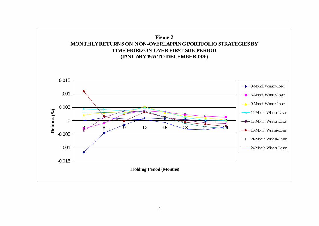
<Figure 2>

13

Figure 2 plots the holding period returns for each of the 8 strategies for the first sub-

period. In contrast to figure 1 it can be seen that the pattern of returns is much flatter, though

again there is a tendency for negative returns for longer ranking periods, and longer holding

periods. Only the 18x3 strategy breaks through the 0.005 per cent barrier, in contrast to

figure 1 where 10 strategies did so.


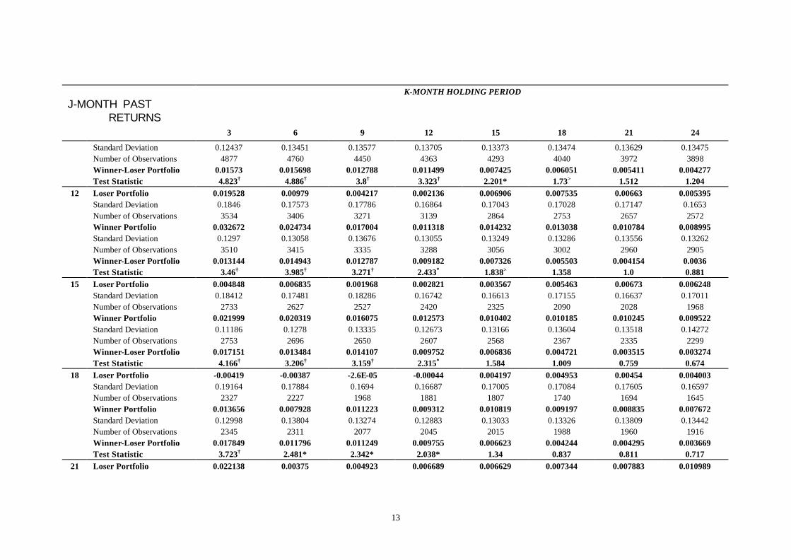
Table III reports the returns for strategies based on non-overlapping observations

for the second series of truncated data from January 1977 to December 1996.

<Table III>

The results presented in Table III and plotted in figure 3 are notably different from

those in Table II. All profits from winner-loser strategies formed from a 3-month ranking

period are positive and significant. The 6-month to 18-month strategies yield positive

returns over all return horizons and up to a 12-month horizon are typically significant. There

is a downward drift to returns on the winner-loser portfolio as the investment horizon

increases, but it is only for the 21-month and 24-month ranking period strategies that there

are any negative returns, and only at long investment horizons. The evidence on profitable

very short-term contrarian strategies has also disappeared. Almost half of the strategies yield

significant positive returns, and break though the 0.005 barrier. The 18x3 strategy is the

most profitable yielding an average annualised return of 23.6 percent, though this is a little

anomalous. A more general pattern seems to be that returns increase at short investment

horizons as we move from the 3-month up to the 9-month ranking periods, and thereafter

start to fall off, though still yielding positive and significant returns. The evidence in this table

is most closely comparable with the results in Liu et al (1999).

<Figure 3>

14

6. Empirical Findings After Controlling for Risk

We expect riskier investments generally to yield higher returns than less risky

investments, so that the results from the previous section, which have shown that returns on

winner portfolios dominate returns on loser portfolios may be because the securities in the

winner portfolio are riskier. We now use the Capital Asset Pricing Model (CAPM) to

quantify of the trade-off between risk and expected return.

With the market portfolio as exogenous and conditional on the realised return of

individual assets, the CAPM model offers a testable prediction of betas. Thus, to investigate

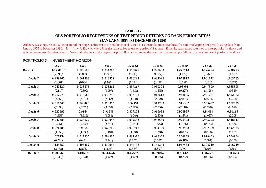
whether a time varying beta explains the phenomenon observed, the Ordinary Least Squares

(OLS) estimator of the slope coefficient in the market model is used to estimate the

respective portfolio betas7 :

Rit = ? i + ? imRmt + eit

where Rit is the realised of portfolio i at time t, Rmt is the realised return of the market

portfolio8 at time t and eit is the zero mean disturbance term. We use this regression method

to obtain the beta of each of the respective decile portfolios. Rather than report the results

for all 64 trading strategies, we concentrate on the symmetric strategies 3x3, 6x6 etc. The t-

statistics in the table are based on the null hypothesis of a beta of unity for the market

portfolio.

<Table IV>

<Figure 4>

Table IV shows that portfolio betas of extreme portfolios (both winner and loser)

are higher across the board for all trading strategies: the t-statistic however, show that the

mid-range betas are more significantly different from unity than compared to those of

7 This is based on the Sharpe-Lintner capital asset pricing model (CAPM) excess-return market model: (Rit - Rf) = ? im + ? im(Rmt - Rf) + eit. The intercept term ? i is transposed as [? im - Rf(? im – 1)] instead of the prevalent Jensen performance index. 8 We use the mean equally-weighted returns of all securities listed on the London Stock Exchange as a

15

extreme winner and loser deciles. There is a tendency for the betas of the loser portfolios to

be slightly higher than the betas for the winner portfolios. In the final row of the table we

report the results of a t-test on the difference in the betas of the winner and loser portfolios:

the evidence that the betas of winner deciles are larger, and hence riskier, than those of loser

deciles, is inconclusive.

We repeated the test on the values of the decile portfolio betas for each of the two

sub-periods, but the results are not reported here. In summary the results from the first sub-

period, January 1955 to December 1976, were similar to the numbers presented in Table

IV: although the betas of the extreme portfolios peak across the board for all trading

strategies, with a tendency for the winner portfolios to have slightly higher betas, this

difference was statistically insignificant. The results of the beta regressions for the second

sub-period January 1977 to December 1996, indicated that the betas of the winner

portfolios are less than the betas of the loser decile. Again though the differences were

insignificant.

The above results demonstrate that returns on trading strategies cannot be

accounted for by a simple adjustment for beta-risk, because the winner and loser portfolios

have similar risk estimates.

broad-based benchmark for the market portfolio.

16

7. Empirical Findings After Controlling for Size

Market capitalisation is defined as the current share price multiplied by the number of

common shares outstanding. Banz (1981) was one of the first to note that firms with lower

market capitalisation (small firms) tend have higher sample mean returns than large firms.

DeBondt and Thaler (1987) argue that the winner-loser phenomena is primary not a size

effect; however, their finding show that on average, winners are twice as large as losers.

Zarowin (1990) also finds that losers are usually smaller than winners based on 3-year

sample periods.

We examine the effect of size on returns by comparing the difference in market

capitalisation between winners and loser portfolios. We concentrate on the second sub-

period of the full sample, since it was over this period that the momentum profits were most

significant. As before, we rank all companies quoted on the London Stock Exchange since

January 1977 based on their 3-month to 24-month historical returns. As previously, stocks

are then sorted into ten equally-weighted deciles in ascending order with decile 1 being the

loser portfolio decile 10 being the winner portfolio. The unique company identification

number of each company is then matched with the LSPD market capitalisation file to obtain

the respective market values,9 and the market capitalisation of each decile is computed by

averaging the market capitalisations of the securities in that decile portfolio. To be included,

a firm must have non-missing values in both the LSPD returns and market capitalisation files.

All market capitalisation figures are adjusted back to 1977 values

<Table V>

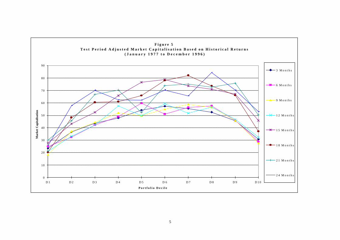
<Figure 5>

Table V report the results obtained by using adjusted rates of market capitalisation for

the period of January 1977 to December 1996. It can be seen that the average size of a

security in each decile rises as we move from the loser decile up to decile 7 or decile 8

across horizon categories. However in the last two to three deciles, average market

9 Zarowin (1990) also perform tests on the effect of size on past period performance on returns. His method ranks stocks based on size first before sorting them into loser and winner deciles within each size decile. Our investigation on the other hand, involves the ranking of stocks by returns followed by the analysis of size for the individual winner and loser deciles. We follow DeBondt and Thaler (1985)

17

capitalisation falls as we move to the winner decile. The market capitalisation of loser

portfolios is smaller than that of winner portfolios across the board. The result of a statistical

test on the equality between these two groups is shown in parenthesis in the last row of

Table V. Our finding are similar to the evidence in Liu et al (1999) where market

capitalisation peaks around the mid-range deciles with loser portfolios smaller in size than

winner portfolios. It is important to note that we can attribute the size effect to explain

excess returns profits only if losers (winners) are consistently bigger (smaller) than winners

(losers) in periods when they outperform each other. In fact while it is true that losers have

a tendency to be smaller than winners, only 3 out of 8 test periods are statistically significant

when tested for equality between these groups. Moreover, statistically significant

momentum profits are only present in holding periods of 3 to 6 months. Consequently, the

difference in size between loser and winner portfolios cannot explain momentum profits,

since we find that the average size of a firm in the winner portfolio is actually larger than the

size of a firm in the loser portfolio. So that although we find some evidence of a size effect in

the UK stock market; nonetheless, this phenomenon can not explain the momentum profits

in the winner-loser portfolio returns.

8. Conclusions

This paper has tested the profitability of momentum trading strategies in the UK stock

market. It did so by examining profits generated by extreme decile portfolios formed on

historical returns. Overall, returns from winner minus loser portfolios are positive and

significant over practically all investment horizons up to 24 months after the portfolio

formation. This is strong evidence of a momentum effect over the short- to medium-term

horizons, where an investor takes a long position on the winner portfolio and sells the loser

portfolio. Earlier work by Clare and Thomas (1995) and Dissanaike (1997) had produced

contradictory findings on the importance of momentum effects in 24-month horizons. Our

findings support the results of Dissanaike (1997) that positive serial correlation is a feature of

the data up to 24-month horizons.

The defining feature of the random walk in stock prices is that successive changes

and Zarowin (1990) in dropping a firm from the test sample once a missing return is detected.

18

are uncorrelated, and deviations from this characteristic imply that the market is not efficient.

However when we split our sample into two sub-periods from 1955-76 and 1977-96, we

found that although the momentum strategy was profitable over the latter period, there was

little evidence of momentum profits in the earlier period. Hence the profitability of

momentum strategies over the entire sample is due to the high profitability of strategies over

the latter half of the sample. This is an important result, because it indicates that positive

serial correlation in UK stock prices is not a general feature of the whole sample, but is only

confined to sub-samples. One possible reason for this result could be due to the less volatile

pre-1976 market as reported by earlier studies on random walk models for stock prices.

Clare et al (1997) suggested that since non-synchronous trading was a problem prior to

April 1981 on the London Stock Exchange, we might expect serial correlation in the earlier

part of the sample. In fact our results report exactly the opposite finding: in the period 1955-

76 there is little evidence in momentum effects (positive serial correlation), while in the

period 1977-1996 there is much stronger evidence of momentum. Hence to the extent that

non-synchronous trading induces positive serial correlation we would have expected

stronger momentum effects in the early period rather than the latter period. Hence non-

synchronous trading cannot be held responsible for the observed momentum effects. This

conclusion is consistent with the findings of Morgan et al (2000) that "non-trading explains,

at most, about one quarter of the autocorrelation in the returns of the smallest value portfolio

in the UK" (page 14)

We have also investigated the notion that winner portfolios were riskier than loser

portfolios, thus accounting for their superior returns. Our results show that returns on

trading strategies cannot be accounted for by a simple adjustment for beta-risk. In addition

although we find some evidence of a size effect in the UK stock market, this phenomenon

can not explain the momentum profits.

In conclusion our results confirm the presence of momentum in the UK market over

the period entire 1955-96. However unlike Liu et al (1999) who suggest that the

momentum profits are a robust feature of sub-samples of the data, we note the strong caveat

that most of these profits were generated over the second half of the sample. The implication

19

is that momentum was not a general feature of the UK stock market over the whole period.

References

Ball, R., and S. Kothari, 1989, Non-Stationary expected returns: implications for tests of market efficiency and serial correlation in returns, Journal of Financial Economics, 25, 51-74. Ball, R., Kothari, S., and J. Shanken, 1995, Problems in measuring portfolio performance: an application to contrarian investment strategies, Journal of Financial Economics, 38, 79-107 Banz, R., 1981, The relation between return and market value of common stocks, Journal of Financial Economics, 9, 3-18. Barber, B., and J. Lyon, 1997, Detecting long-run abnormal stock returns: the empirical power and specification of test statistics, Journal of Financial Economics, 43, 341-372. Barberis, N., Shleifer, A., and R. Vishny, 1998, A model of investor sentiment, Journal of Financial Economics, 49, 307-343. Berk, J., Green, R., and V. Naik, 1999, Optimal investment, growth options and security returns, Journal of Finance, 54, 1553-1607. Chan, K, 1988, On contrarian investment strategy, Journal of Business, 61, 147-163. Chan, K. C., Jegadeesh N., and J. Lakonishok, 1996, Momentum strategies, Journal of Finance, 51, 1681-1713. Chopra, N., Lakonishok, J., and J. Ritter, 1992, Measuring abnormal performance, Journal of Financial Economics, 31, 235-268. Clare, A., Morgan G., and S. Thomas, 1997, Direct evidence of non-synchronous trading on the London Stock Exchange, University of Southampton, mimeo. Clare, A., and S. Thomas, 1995, The overreaction hypothesis and the UK stockmarket, Journal of Business Finance and Accounting, 22, 961-973. Conrad, J., and G. Kaul, 1993, Long-term market overreaction or biases in computed returns?, Journal of Finance, 48, 39-63. Conrad, J., and G. Kaul, 1998, An anatomy of trading strategies, Review of Financial Studies, 11, 489-519. De Bondt, W., and R. Thaler, 1985, Does the stock market overreact?, Journal of Finance, 40, 793-805.

20

De Bondt, W, and R. Thaler, 1987, Further evidence of investor overreaction and stock market seasonality, Journal of Finance, 42, 557-581. De Long, B., Shleifer, A., Summers, L., and R. Waldmann, 1990, Positive feedback investment strategies and destabilizing rational speculation, Journal of Finance, 45, 379-395. Daniel, K., Hirshleifer, D., and A. Subrahmanyam, 1998, Investor psychology and security market under- and overreactions, Journal of Finance, 53, 1839-1885. Dimson, E., and P. Marsh, 1986, Event study methodologies and the size effect: the case of UK press recommendations, Journal of Financial Economics, 17, 113-142. Dissanaike, G., 1997, Do stock market investors overreact? Journal of Business Finance and Accounting, 24, 27-49. Fama, E., and K. French, 1988, Permanent and temporary components of stock prices, Journal of Political Economy, 96, 246-273. Fama, E., and K. French, 1996, Multifactor explanations of asset pricing anomalies, Journal of Finance, 51, 55-84. Grinblatt, M., and S. Titman, 1989, Mutual fund performance: an analysis of quarterly portfolio holdings, Journal of Business, 62, 394-415. Grundy, B., and J. Martin, 1998, Understanding the nature of risks and the source of the rewards to momentum investing, Working Paper, University of Pennsylvania. Hong, H., and J. Stein, 1999, A unified theory of underreaction, momentum trading and overreaction in asset markets, Journal of Finance, 53, 1935-1974. Hong, H., Lim, T., and J. Stein, 2000, Bad news travels slowly: size, analyst coverage, and the profitability of momentum strategies, Journal of Finance, 55, 265-295. Jegadeesh, N., 1990, Evidence of predictable behaviour of security returns, Journal of Finance, 45, 881-898. Jegadeesh N., and S. Titman, 1993, Returns to buying winners and selling losers: implications for stock market efficiency, Journal of Finance, 48, 65-91. Jegadeesh N., and S. Titman, 1995, Overreaction, delayed reaction, and contrarian profits, Review of Financial Studies, 8, 973-993. Kaul, G., and M. Nimalendran, 1990, Price reversals: bid-ask errors or market overreaction?, Journal of Financial Economics, 28, 67-93. Kothari, S., and J. Warner, 1997, Measuring long-horizon performance: abnormal returns,

21

Journal of Financial Economics, 43, 301-339. Liu, W., Norman, S., and X. Xu, 1999, The profitability of momentum investing, Journal of Business Finance and Accounting, 26, 1043-1091. Lo, A., and A. MacKinlay, 1988, Stock prices do not follow random walks: evidence from a simple specification test, The Review of Financial Studies, 41-66. Lo, A., and A. MacKinlay, 1990, When are contrarian profits due to stock market overreaction?, Review of Financial Studies, 3, 175-205. MacDonald, R., and D. Power, 1991, Persistence in UK stock market returns: an aggregated and disaggregated perspective, in: M. Taylor, ed., Money and Financial Markets (Basil Blackwell). Morgan, G., Smith, P., and S. Thomas, 2000, Portfolio return autocorrelation and non-synchronous trading in UK equities, University of York Discussion Paper, 2000/46 Moskowitz, T., and M. Grinblatt, 1999, Do industries explain momentum?, Journal of Finance, 54, 1249-1290. Poterba, J., and L. Summers, 1988, Mean reversion in stock prices, Journal of Financial Economics, 27-59. Power, D., Lonie A., and R. Lonie, 1991, Some UK evidence of stock market overreaction, British Accounting Review, June, 149-170. Richards, A., 1997, Winner-Loser reversals in national stock market indices: can they be explained? Journal of Finance, 52, 2129-2144. Rouwenhorst, K., 1998, International momentum strategies, Journal of Finance, 53, 267-284. Smith, J, and S. Yadav, 1996, A comparison of alternative covariance matrices for models with overlapping observations, Journal of International Money and Finance, 15, 813-823. Zarowin, P., 1990, Size, seasonality, and stock market overreaction, Journal of Financial and Quantitative Analysis, 25, 113-125.

3 6 9 12 15 18 21 24

-0.004

-0.002

0

0.002

0.004

0.006

0.008

0.01

0.012

Ret

urns

(%)

Holding Period (Months)

Figure 1MONTHLY RETURNS ON NON-OVERLAPPING PORTFOLIO STRATEGIES BY

TIME HORIZON(JANUARY 1955 TO DECEMBER 1996)

24-Month Winner-Loser








2

Figure 2MONTHLY RETURNS ON NON-OVERLAPPING PORTFOLIO STRATEGIES BY

TIME HORIZON OVER FIRST SUB-PERIOD (JANUARY 1955 TO DECEMBER 1976)

-0.015

-0.01

-0.005

0

0.005

0.01

0.015

3 6 9 12 15 18 21 24


Ret

urns

(%)









3

Figure 3 MONTHLY RETURNS ON NON-OVERLAPPING PORTFOLIO STRATEGIES BY

TIME HORIZON SECOND SUB-PERIOD (JANUARY 1977 TO DECEMBER 1996)

-0.005

0

0.005

0.01

0.015

0.02

3 6 9 12 15 18 21 24


Ret

urns

(%)









4

D 1 D 2 D 3 D 4 D 5 D 6 D 7 D 8 D 9 D10

3 x 3

9 x 9

15 x 1521 x 21

0.3

0.5

0.7

0.9

1.1

1.3

Bet

a

Portfolio Decile

Figure 4OLS PORTFOLIO REGRESSIONS OF TEST PERIOD RETURNS ON RANK PERIOD

BETAS (JANUARY 1955 TO DECEMBER 1996)

3 x 3 6 x 6

9 x 9 12 x 12

15 x 15 18 x 18

21 x 21 24 x 24

5

F i g u r e 5T e s t P e r i o d A d j u s t e d M a r k e t C a p i t a l i s a t i o n B a s e d o n H i s t o r i c a l R e t u r n s

( J a n u a r y 1 9 7 7 t o D e c e m b e r 1 9 9 6 )

0

10

20

30

40

50

60

70

80

90

D 1 D 2 D 3 D 4 D 5 D 6 D 7 D 8 D 9 D 1 0

P o r t f o l i o D e c i l e

Mar

ket

Cap

italis

atio

n

3 M o n t h s

6 M o n t h s

9 M o n t h s

1 2 M o n t h s

1 5 M o n t h s

1 8 M o n t h s

2 1 M o n t h s

2 4 M o n t h s

6

TABLE I MONTHLY RETURNS ON NON-OVERLAPPING PORTFOLIO STRATEGIES BY TIME HORIZON

(JANUARY 1955 TO DECEMBER 1996) Stocks are sorted and ranked in ascending order based on their respective J-month lagged returns. Stocks are further divided into ten equally weighted deciles. The top decile is the ‘loser’ portfolio and the bottom decile ‘winner’ portfolio. In month t, the strategy goes short on the loser portfolio and long on the winner portfolio. Thus, based on J-months of historical data, portfolios are held on for period of K-months and executed in month t. Buy-and-hold returns are computed for both the winner and loser portfolios.

J-MONTH PAST RETURNS K-MONTH HOLDING PERIOD

3 6 9 12 15 18 21 24

3 Loser Portfolio 0.010855 0.007095 0.005808 0.005659 0.006458 0.007177 0.007771 0.007809 Standard Deviation 0.16212 0.15551 0.15244 0.15321 0.15365 0.15178 0.14989 0.14919 Number of Observations 29578 28578 27604 26652 25812 24933 24179 22630 Winner Portfolio 0.006575 0.008734 0.009717 0.010512 0.010008 0.009659 0.009536 0.0098 Standard Deviation 0.13662 0.13434 0.13415 0.13473 0.13455 0.13585 0.13441 0.13394 Number of Observations 28530 27535 26732 26013 25321 24685 24055 22744

Winner-Loser Portfolioa

-0.00428 0.001639 0.003908 0.004853 0.00355 0.002482 0.001765 0.001991

Test Statisticb -3.44† 1.315 3.098† 3.792† 2.751† 1.897> 1.346 1.482 6 Loser Portfolio 0.007999 0.004404 0.004231 0.004631 0.005644 0.006398 0.007139 0.007357 Standard Deviation 0.16862 0.16067 0.15652 0.15807 0.15625 0.1556 0.1534 0.15299 Number of Observations 14524 13906 13511 12952 12591 12064 11759 11269 Winner Portfolio 0.011329 0.011344 0.012305 0.011654 0.011088 0.010368 0.010556 0.010257 Standard Deviation 0.13375 0.13139 0.13458 0.13225 0.1336 0.1346 0.13307 0.13343 Number of Observations 14085 13523 13255 12805 12580 12183 11959 11539 Winner-Loser Portfolio 0.003329 0.00694 0.008074 0.007023 0.005444 0.003969 0.003417 0.0029 Test Statistic 1.881> 3.917† 4.47† 3.854† 2.953† 2.12* 1.8>

1.531 9 Loser Portfolio 0.004286 0.002706 0.003782 0.004303 0.004952 0.00654 0.006875 0.007325 Standard Deviation 0.17132 0.16205 0.15984 0.16169 0.16017 0.15657 0.1576 0.15312 Number of Observations 9316 9036 8755 8288 8089 7868 7501 7305 Winner Portfolio 0.010683 0.012223 0.012188 0.011753 0.010263 0.010224 0.01007 0.009415

7


3 6 9 12 15 18 21 24

Standard Deviation 0.13202 0.12615 0.13029 0.13616 0.13446 0.13394 0.1367 0.13665 Number of Observations 9126 8925 8782 8421 8288 8150 7827 7683 Winner-Loser Portfolio 0.006397 0.009518 0.008405 0.007449 0.00531 0.003683 0.003195 0.00209 Test Statistic 2.904† 4.4† 3.801† 3.238† 2.308† 1.598 1.358 0.886

12 Loser Portfolio 0.015929 0.001601 -4.8E-05 0.004617 0.007754 0.006158 0.005862 0.007992 Standard Deviation 0.16857 0.16431 0.15954 0.15626 0.15291 0.15493 0.15424 0.15241 Number of Observations 6889 6680 6459 6092 5915 5736 5595 5299 Winner Portfolio 0.024624 0.01418 0.009957 0.011893 0.013213 0.010556 0.009071 0.009881 Standard Deviation 0.12651 0.12545 0.13155 0.12923 0.12903 0.13167 0.13244 0.12979 Number of Observations 6797 6632 6515 6222 6115 6000 5906 5629 Winner-Loser Portfolio 0.008695 0.012579 0.010005 0.007276 0.005459 0.004399 0.00321 0.001889 Test Statistic 3.447† 5.005† 3.864† 2.767† 2.068† 1.649> 1.201 0.701

15 Loser Portfolio -0.00211 -0.00158 0.001334 0.002872 0.006297 0.005721 0.006396 0.007108 Standard Deviation 0.18065 0.16586 0.16201 0.16429 0.16225 0.15777 0.15347 0.15145 Number of Observations 5520 5155 4995 4842 4694 4562 4297 4166 Winner Portfolio 0.004555 0.004876 0.007215 0.008756 0.009888 0.00847 0.00738 0.007387 Standard Deviation 0.13399 0.13492 0.13263 0.13654 0.13452 0.13307 0.13156 0.13084 Number of Observations 5471 5186 5115 5031 4937 4843 4575 4500 Winner-Loser Portfolio 0.006665 0.006452 0.00588 0.005884 0.00359 0.002749 0.000983 0.000279 Test Statistic 2.314* 2.194* 1.995* 1.953> 1.196 0.92 0.325 0.092

18 Loser Portfolio 0.00947 0.008257 0.009997 0.008203 0.007521 0.00831 0.009295 0.009741 Standard Deviation 0.16901 0.1584 0.1547 0.16074 0.158 0.15863 0.15597 0.14972 Number of Observations 4389 4256 4108 3830 3736 3640 3532 3414 Winner Portfolio 0.016939 0.01423 0.014068 0.012544 0.010091 0.009073 0.009121 0.008926 Standard Deviation 0.12484 0.11835 0.12715 0.13039 0.13392 0.13391 0.13641 0.13507 Number of Observations 4359 4272 4219 3956 3910 3838 3778 3712 Winner-Loser Portfolio 0.00747 0.005973 0.004071 0.004341 0.00257 0.000763 -0.00017 -0.00081 Test Statistic 2.383* 1.94> 1.278 1.312 0.769 0.228 -0.05 -0.24

21 Loser Portfolio 0.003773 0.00125 0.00132 0.006628 0.007861 0.007594 0.009102 0.009404 Standard Deviation 0.1703 0.16487 0.16376 0.16748 0.1526 0.15212 0.14737 0.14426 Number of Observations 3679 3575 3452 3189 3093 3000 2907 2828 Winner Portfolio 0.011318 0.008125 0.006803 0.011126 0.009774 0.008452 0.009213 0.008749

8


3 6 9 12 15 18 21 24

Standard Deviation 0.11076 0.12163 0.12493 0.12598 0.12261 0.13063 0.13036 0.13037 Number of Observations 3677 3605 3539 3307 3251 3193 3135 3089 Winner-Loser Portfolio 0.007545 0.006875 0.005483 0.004498 0.001913 0.000858 0.000111 -0.00065 Test Statistic 2.293* 2.031* 1.591 1.263 0.541 0.236 0.031 -0.18

24 Loser Portfolio 0.036526 0.015561 0.013223 0.015504 0.013819 0.010867 0.008803 0.01051 Standard Deviation 0.17083 0.16335 0.15552 0.16025 0.15912 0.15671 0.15904 0.15449 Number of Observations 3219 3109 3014 2771 2689 2608 2539 2456 Winner Portfolio 0.035315 0.020914 0.016328 0.015762 0.013609 0.010241 0.007961 0.008804 Standard Deviation 0.11703 0.12311 0.12224 0.12176 0.12884 0.13101 0.135 0.13429 Number of Observations 3222 3168 3109 2879 2831 2777 2745 2706 Winner-Loser Portfolio -0.00121 0.005353 0.003105 0.000258 -0.00021 -0.00063 -0.00084 -0.00171 Test Statistic -0.34 1.474 0.851 0.068 -0.05 -0.16 -0.21 -0.43

a The trading strategies are replicated for each stated period and the mean returns shown for each horizon is the log normal average of all non-overlapping replications. † Significant at the 99% level * Significant at the 95% level > Significant at the 90% level.

9

TABLE II MONTHLY RETURNS ON NON-OVERLAPPING PORTFOLIO STRATEGIES BY TIME HORIZON

OVER FIRST SUB-PERIOD (JANUARY 1955 TO DECEMBER 1976) Stocks are sorted and ranked in ascending order based on their respective J-month lagged returns. Stocks are further divided into ten equally weighted deciles. The top decile is the ‘loser’ portfolio and the bottom decile ‘winner’ portfolio. In month t, the strategy goes short on the loser portfolio and long on the winner portfolio. Thus, based on J-months of historical data, portfolios are held on for period of K-months and executed in month t. Buy-and-hold returns are computed for both the winner and loser portfolios.

J-MONTH PAST RETURNS

K-MONTH HOLDING PERIOD

3 6 9 12 15 18 21 24

3 Loser Portfolio 0.014643 0.010182 0.008505 0.007209 0.007106 0.007218 0.007472 0.007368 Standard Deviation 0.1385 0.13228 0.1282 0.12969 0.13028 0.12827 0.12765 0.12582 Number of Observations 12842 12412 11971 11517 11091 10657 10271 9962 Winner Portfolio 0.002937 0.005646 0.006986 0.008188 0.007819 0.00764 0.007546 0.007577 Standard Deviation 0.1291 0.12567 0.12418 0.12604 0.12538 0.1243 0.12542 0.12376 Number of Observations 12357 11841 11407 11012 10621 10234 9851 9523 Winner-Loser Portfolioa -0.01171 -0.00454 -0.00152 0.000979 0.000713 0.000422 7.46E-05 0.000208 Test Statisticb -6.94† -2.74† -0.92 0.575 0.411 0.242 0.042 0.116 6 Loser Portfolio 0.011165 0.00891 0.006768 0.005532 0.006003 0.005837 0.006576 0.006194 Standard Deviation 0.14438 0.13424 0.13469 0.13362 0.13485 0.13204 0.13276 0.12922 Number of Observations 6333 6000 5886 5552 5446 5132 5048 4812 Winner Portfolio 0.008189 0.007967 0.009195 0.009263 0.009213 0.008077 0.008137 0.007436 Standard Deviation 0.13063 0.12084 0.12827 0.12585 0.12606 0.12671 0.1266 0.12677 Number of Observations 6082 5725 5633 5312 5242 4918 4842 4620 Winner-Loser Portfolio -0.00298 -0.00094 0.002427 0.003732 0.00321 0.00224 0.001561 0.001242 Test Statistic -1.2 -0.4 0.99 1.499 1.272 0.868 0.599 0.471 9 Loser Portfolio -0.00142 0.004138 0.00511 0.002353 0.00463 0.006079 0.005329 0.006327 Standard Deviation 0.14765 0.13269 0.13349 0.13781 0.13345 0.12873 0.1329 0.12747 Number of Observations 3973 3897 3815 3514 3459 3404 3224 3166 Winner Portfolio 0.000559 0.007175 0.007864 0.007691 0.007602 0.00773 0.006414 0.006555 Standard Deviation 0.1268 0.12402 0.1273 0.13483 0.12962 0.12537 0.1368 0.13573

10



3 6 9 12 15 18 21 24

Number of Observations 3842 3774 3726 3431 3376 3325 3118 3059 Winner-Loser Portfolio 0.001976 0.003037 0.002754 0.005339 0.002972 0.001651 0.001085 0.000228 Test Statistic 0.635 1.036 0.917 1.632 0.934 0.533 0.32 0.068

12 Loser Portfolio 0.013993 0.003012 0.001836 0.004769 0.007176 0.005729 0.005723 0.006792 Standard Deviation 0.14815 0.13698 0.14035 0.13554 0.13454 0.13247 0.13524 0.12927 Number of Observations 2947 2884 2817 2561 2506 2457 2414 2238 Winner Portfolio 0.018436 0.007285 0.005512 0.009642 0.010564 0.006951 0.005884 0.006784 Standard Deviation 0.12421 0.11654 0.12648 0.12741 0.12606 0.12607 0.12992 0.12768 Number of Observations 2870 2805 2769 2484 2440 2404 2373 2191 Winner-Loser Portfolio 0.004443 0.004273 0.003676 0.004873 0.003388 0.001222 0.000162 -7.7E-06 Test Statistic 1.241 1.268 1.029 1.316 0.914 0.329 0.042 -0

15 Loser Portfolio 0.004338 -0.00467 0.000738 0.003399 0.006676 0.005864 0.00416 0.004803 Standard Deviation 0.15841 0.14396 0.14426 0.14983 0.14145 0.13275 0.13053 0.12566 Number of Observations 2416 2354 2091 2049 2015 1985 1947 1780 Winner Portfolio 0.000512 -0.00349 0.004428 0.006658 0.007838 0.006075 0.003379 0.003764 Standard Deviation 0.13103 0.12944 0.13194 0.14442 0.13431 0.12808 0.13063 0.13162 Number of Observations 2364 2321 2057 2025 1987 1946 1912 1752 Winner-Loser Portfolio -0.00383 0.001183 0.00369 0.003259 0.001163 0.000211 -0.00078 -0.00104 Test Statistic -0.91 0.296 0.86 0.707 0.267 0.051 -0.19 -0.24

18 Loser Portfolio 0.003952 0.011908 0.0129 0.006823 0.007173 0.008132 0.008749 0.010207 Standard Deviation 0.14765 0.12899 0.12692 0.12756 0.12729 0.12673 0.13422 0.12836 Number of Observations 1873 1831 1791 1632 1606 1584 1554 1520 Winner Portfolio 0.01483 0.013526 0.012751 0.01 0.008624 0.007514 0.007371 0.008138 Standard Deviation 0.121 0.11614 0.12556 0.12708 0.12835 0.12922 0.13917 0.13509 Number of Observations 1834 1797 1777 1599 1581 1558 1529 1497 Winner-Loser Portfolio 0.010878 0.001619 -0.00015 0.003177 0.001451 -0.00062 -0.00138 -0.00207 Test Statistic 2.456* 0.397 -0.04 0.709 0.32 -0.14 -0.28 -0.43

21 Loser Portfolio 0.004556 0.000736 0.002287 0.007783 0.007954 0.008995 0.009889 0.009999 Standard Deviation 0.14225 0.14526 0.13243 0.12062 0.12868 0.13178 0.12964 0.12202 Number of Observations 1561 1526 1492 1336 1309 1281 1252 1229

11



3 6 9 12 15 18 21 24

Winner Portfolio 0.007799 0.003722 0.005063 0.011461 0.00925 0.007912 0.007544 0.007211 Standard Deviation 0.11185 0.12758 0.1285 0.11986 0.12735 0.13499 0.13321 0.13339 Number of Observations 1538 1503 1479 1305 1284 1262 1238 1219 Winner-Loser Portfolio 0.003244 0.002986 0.002776 0.003677 0.001296 -0.00108 -0.00235 -0.00279 Test Statistic 0.706 0.601 0.58 0.786 0.258 -0.2 -0.45 -0.54

24 Loser Portfolio 0.027714 0.01057 0.014079 0.013923 0.013087 0.011503 0.008787 0.008498 Standard Deviation 0.15381 0.12816 0.13456 0.1407 0.1449 0.13786 0.13689 0.1226 Number of Observations 1267 1235 1212 1185 1155 1129 1107 953 Winner Portfolio 0.027649 0.011678 0.014706 0.014239 0.012342 0.008295 0.005425 0.006207 Standard Deviation 0.11817 0.11825 0.12115 0.12686 0.13537 0.13698 0.13869 0.13841 Number of Observations 1248 1229 1213 1186 1164 1146 1133 986 Winner-Loser Portfolio -6.4E-05 0.001107 0.000627 0.000316 -0.00074 -0.00321 -0.00336 -0.00229 Test Statistic -0.01 0.223 0.121 0.057 -0.13 -0.56 -0.58 -0.39

a The trading strategies are replicated for each stated period and the mean returns shown for each horizon is the log normal average of all non-overlapping replications. † Significant at the 99% level * Significant at the 95% level

12

TABLE III MONTHLY RETURNS ON NON-OVERLAPPING PORTFOLIO STRATEGIES BY TIME HORIZON

SECOND SUB-PERIOD (JANUARY 1977 TO DECEMBER 1996) Stocks are sorted and ranked in ascending order based on their respective J-month lagged returns. Stocks are further divided into ten equally weighted deciles. The top decile is the ‘loser’ portfolio and the bottom decile ‘winner’ portfolio. In month t, the strategy goes short on the loser portfolio and long on the winner portfolio. Thus, based on J-months of historical data, portfolios are held on for period of K-months and executed in month t. Buy-and-hold returns are computed for both the winner and loser portfolios.



3 6 9 12 15 18 21 24

3 Loser Portfolio 0.004213 0.002611 0.002888 0.002881 0.004192 0.004822 0.005588 0.005576 Standard Deviation 0.17542 0.172 0.16878 0.16851 0.16847 0.1675 0.1651 0.16415 Number of Observations 15641 14897 14198 13536 12881 12302 11767 11267 Winner Portfolio 0.011028 0.011142 0.011429 0.011711 0.010814 0.009993 0.009442 0.009566 Standard Deviation 0.13951 0.14043 0.13976 0.14091 0.1417 0.14231 0.14147 0.14135 Number of Observations 15151 14482 13918 13395 12917 12506 12082 11685 Winner-Loser Portfolioa 0.006815 0.008531 0.008542 0.00883 0.006623 0.00517 0.003855 0.00399 Test Statisticb 3.779† 4.662† 4.626† 4.667† 3.416† 2.618† 1.934> 1.97* 6 Loser Portfolio 0.006795 0.001014 0.002766 0.002506 0.00477 0.004621 0.005859 0.005567 Standard Deviation 0.18196 0.17325 0.1722 0.16848 0.17096 0.16839 0.16906 0.16534 Number of Observations 7541 7266 6819 6578 6181 5972 5635 5441 Winner Portfolio 0.01905 0.013494 0.015628 0.013648 0.012974 0.010765 0.011536 0.010519 Standard Deviation 0.13196 0.13474 0.13834 0.13415 0.13773 0.13856 0.13929 0.13738 Number of Observations 7375 7174 6811 6670 6369 6268 5992 5861 Winner-Loser Portfolio 0.012255 0.01248 0.012862 0.011142 0.008204 0.006144 0.005677 0.004952 Test Statistic 4.716† 4.835† 4.807† 4.207† 2.955† 2.198* 1.969* 1.725> 9 Loser Portfolio -0.0031 -0.00115 0.001787 0.001251 0.003879 0.004761 0.004621 0.005563 Standard Deviation 0.19193 0.176 0.1777 0.17995 0.17125 0.17056 0.17181 0.16722 Number of Observations 4933 4750 4396 4224 4066 3756 3632 3516 Winner Portfolio 0.01263 0.014547 0.014575 0.01275 0.011304 0.010812 0.010032 0.00984

13



3 6 9 12 15 18 21 24

Standard Deviation 0.12437 0.13451 0.13577 0.13705 0.13373 0.13474 0.13629 0.13475 Number of Observations 4877 4760 4450 4363 4293 4040 3972 3898 Winner-Loser Portfolio 0.01573 0.015698 0.012788 0.011499 0.007425 0.006051 0.005411 0.004277 Test Statistic 4.823† 4.886† 3.8† 3.323† 2.201* 1.73> 1.512 1.204

12 Loser Portfolio 0.019528 0.00979 0.004217 0.002136 0.006906 0.007535 0.00663 0.005395 Standard Deviation 0.1846 0.17573 0.17786 0.16864 0.17043 0.17028 0.17147 0.1653 Number of Observations 3534 3406 3271 3139 2864 2753 2657 2572 Winner Portfolio 0.032672 0.024734 0.017004 0.011318 0.014232 0.013038 0.010784 0.008995 Standard Deviation 0.1297 0.13058 0.13676 0.13055 0.13249 0.13286 0.13556 0.13262 Number of Observations 3510 3415 3335 3288 3056 3002 2960 2905 Winner-Loser Portfolio 0.013144 0.014943 0.012787 0.009182 0.007326 0.005503 0.004154 0.0036 Test Statistic 3.46† 3.985† 3.271† 2.433* 1.838> 1.358 1.0 0.881

15 Loser Portfolio 0.004848 0.006835 0.001968 0.002821 0.003567 0.005463 0.00673 0.006248 Standard Deviation 0.18412 0.17481 0.18286 0.16742 0.16613 0.17155 0.16637 0.17011 Number of Observations 2733 2627 2527 2420 2325 2090 2028 1968 Winner Portfolio 0.021999 0.020319 0.016075 0.012573 0.010402 0.010185 0.010245 0.009522 Standard Deviation 0.11186 0.1278 0.13335 0.12673 0.13166 0.13604 0.13518 0.14272 Number of Observations 2753 2696 2650 2607 2568 2367 2335 2299 Winner-Loser Portfolio 0.017151 0.013484 0.014107 0.009752 0.006836 0.004721 0.003515 0.003274 Test Statistic 4.166† 3.206† 3.159† 2.315* 1.584 1.009 0.759 0.674

18 Loser Portfolio -0.00419 -0.00387 -2.6E-05 -0.00044 0.004197 0.004953 0.00454 0.004003 Standard Deviation 0.19164 0.17884 0.1694 0.16687 0.17005 0.17084 0.17605 0.16597 Number of Observations 2327 2227 1968 1881 1807 1740 1694 1645 Winner Portfolio 0.013656 0.007928 0.011223 0.009312 0.010819 0.009197 0.008835 0.007672 Standard Deviation 0.12998 0.13804 0.13274 0.12883 0.13033 0.13326 0.13809 0.13442 Number of Observations 2345 2311 2077 2045 2015 1988 1960 1916 Winner-Loser Portfolio 0.017849 0.011796 0.011249 0.009755 0.006623 0.004244 0.004295 0.003669 Test Statistic 3.723† 2.481* 2.342* 2.038* 1.34 0.837 0.811 0.717

21 Loser Portfolio 0.022138 0.00375 0.004923 0.006689 0.006629 0.007344 0.007883 0.010989

14



3 6 9 12 15 18 21 24

Standard Deviation 0.17979 0.17822 0.17724 0.17948 0.18106 0.18693 0.19307 0.1827 Number of Observations 1929 1867 1793 1569 1502 1450 1398 1359 Winner Portfolio 0.020061 0.011026 0.011533 0.010863 0.007566 0.006762 0.007648 0.008908 Standard Deviation 0.11133 0.13779 0.13549 0.1306 0.1314 0.1363 0.1371 0.13198 Number of Observations 1945 1909 1869 1672 1644 1623 1604 1581 Winner-Loser Portfolio -0.00208 0.007277 0.006609 0.004174 0.000937 -0.00058 -0.00023 -0.00208 Test Statistic -0.43 1.401 1.264 0.753 0.165 -0.1 -0.04 -0.35

24 Loser Portfolio 0.041998 0.025748 0.021317 0.011708 0.011556 0.010508 0.00694 0.007534 Standard Deviation 0.18399 0.18498 0.17029 0.16859 0.17537 0.16702 0.17301 0.16672 Number of Observations 1556 1501 1443 1390 1351 1295 1244 1203 Winner Portfolio 0.045846 0.031251 0.022324 0.012167 0.012207 0.010478 0.007094 0.007173 Standard Deviation 0.11721 0.11992 0.12898 0.11942 0.12764 0.12416 0.13198 0.13113 Number of Observations 1569 1546 1522 1494 1474 1448 1426 1409 Winner-Loser Portfolio 0.003848 0.005503 0.001007 0.000459 0.000651 -3E-05 0.000154 -0.00036 Test Statistic 0.697 0.971 0.181 0.084 0.112 -0.01 0.026 -0.06

a The trading strategies are replicated for each stated period and the mean returns shown for each horizon is the log normal average of all non-overlapping replications. † Significant at the 99% level * Significant at the 95% level > Significant at the 90% level

15

TABLE IV OLS PORTFOLIO REGRESSIONS OF TEST PERIOD RETURNS ON RANK PERIOD BETAS

(JANUARY 1955 TO DECEMBER 1996) Ordinary Least Squares (OLS) estimator of the slope coefficient in the market model is used to estimate the respective betas for non-overlapping test periods using data from January 1955 to December 1996: Rit = ? im + ? imRmt + eit where Rit is the realised log return on portfolio a i at time t, Rmt is the realised log return on market porfoliob at time t and eit is the zero mean disturbance term. We obtain the beta of the respective portfolios by regressing the return on the market porfolio on the mean return of portfolio i at time t.

PORTFOLIO ? INVESTMENT HORIZON 3 x 3 6 x 6 9 x 9 12 x 12 15 x 15 18 x 18 21 x 21 24 x 24

Decile 1 1.176091c 1.208653 1.254213 1.193675 1.223593 1.277913 1.175794 1.240793 (2.195)d (1.863) (1.962) (1.210) (1.587) (1.170) (0.763) (1.328)

Decile 2 0.999965 1.001493 1.043352 1.016221 1.021921 1.078817 1.001172 1.063785 -(0.001) (0.034) (0.925) (0.244) (0.437) (0.757) (0.016) (0.877)

Decile 3 0.940137 0.938175 0.973212 0.957217 0.950305 0.98991 0.947399 0.985305 -(2.117) -(2.302) -(0.997) -(1.413) -(1.595) -(0.227) -(1.828) -(0.529)

Decile 4 0.917579 0.913568 0.936796 0.933152 0.918518 0.942095 0.931281 0.942562 -(4.366) -(4.216) -(2.862) -(3.538) -(2.679) -(2.861) -(2.633) -(3.458)

Decile 5 0.916266 0.909406 0.918353 0.92491 0.917793 0.916302 0.935497 0.922999 -(5.693) -(4.576) -(3.358) -(2.995) -(2.706) -(2.116) -(1.726) -(2.629)

Decile 6 0.922992 0.9164 0.91243 0.927201 0.919953 0.909967 0.94464 0.91115 -(4.856) -(3.919) -(3.083) -(2.049) -(2.574) -(1.571) -(1.057) -(2.208)

Decile 7 0.942888 0.934627 0.920046 0.932553 0.933659 0.920593 0.955298 0.918017 -(2.751) -(2.533) -(2.541) -(1.551) -(1.983) -(1.136) -(0.733) -(1.576)

Decile 8 0.971089 0.9665 0.945709 0.958718 0.954159 0.933903 0.982389 0.942985 -(1.053) -(1.035) -(1.489) -(0.788) -(1.260) -(0.851) -(0.278) -(1.001)

Decile 9 1.027154 1.017155 0.984969 1.017976 1.012939 0.966293 1.018469 0.994204 (0.721) (0.421) -(0.341) (0.306) (0.265) -(0.415) (0.297) -(0.100)

Decile 10 1.185659 1.193482 1.110957 1.137798 1.145241 1.067488 1.108219 1.076219 (3.138) (2.875) (1.649) (2.583) (1.890) (0.909) (1.605) (1.662)

D1 - D10 0.009568 -0.015171 -0.143256 -0.055877 -0.078352 -0.210425 -0.067575 -0.164574 (0.033)e -(0.041) -(0.422) -(0.127) -(0.185) -(0.752) -(0.186) -(0.354)

16

a To be included in each test period, a security must have non-missing returns both the ranking and holding period. On each portfolio formation date, companies are sorted and ranked based on the holding period returns and allocated to one of the ten deciles; with the extreme top decile as the ‘loser’ portfolio and the extreme bottom decile as the ‘winner’ portfolio. b We use the mean equally-weighted returns of all companies listed on the London Stock Exchange with non-missing returns as a broad-based benchmark for the market porfolio. c Securities are ranked based on past returns and assigned in equal numbers to ten portfolios. For each decile, a pooled regression over the returns was performed to estimate the beta for the respective portfolios. d Test statistic for null hypothesis of portfolio having a unity beta (i.e., market portfolio) using the Newey-West standard error. e Test statistic for null hypothesis of equality between betas of winner portfolio (decile 10) and loser portfolio (decile 1) using Newey-West standard errors. † Significant at the 95% level * Significant at the 95% level > Significant at the 90% level.

17

TABLE V TEST PERIOD ADJUSTED^ MARKET CAPITALISATION* BASED ON HISTORICAL RETURNS

(JANUARY 1977 TO DECEMBER 1996)

Using yearly market capitalisation data from the LSPD tapes, we first rank all British registered companies quoted on the London Stock Exchange based on their historical returns on each portfolio formation date. The stocks are further sorted into ten equally-weighted deciles in ascending order; that is, the top decile (decile 1) is the loser portfolio and the bottom decile (decile 10) is the winner portfolio. The unique company identification number of each company is then matched with the LSPD market capitalisation file to obtain the subsequent average market capitalisation for the following year for each decile portfolioa.

PORTFOLIO HISTORICAL HORIZON 3 MONTHS 6 MONTHS 9 MONTHS 12 MONTHS 15 MONTHS 18 MONTHS 21 MONTHS 24 MONTHS

DECILE 1 23.4123 24.87831 18.19055 21.06481 27.62423 20.14545 30.01112 25.41228

DECILE 2 36.46783 32.45337 37.11601 33.18265 43.09243 48.26271 45.5545 57.8808

DECILE 3 43.63281 42.06987 44.315 42.06309 52.54118 60.44807 66.82402 70.14192

DECILE 4 47.96091 49.08309 52.03454 57.70418 65.95312 60.9877 70.39863 62.42256

DECILE 5 54.2462 59.82295 49.90724 49.9073 76.64269 65.95816 52.42564 62.26746

DECILE 6 57.36148 51.07165 55.02303 59.43116 78.75453 78.03669 73.91827 70.383

DECILE 7 55.54834 56.3996 58.86735 51.81883 73.72482 82.0841 75.09611 65.60038

DECILE 8 52.6569 57.59863 56.76366 56.68794 70.93657 73.67321 72.64594 84.48552

DECILE 9 45.55809 45.62096 45.83683 46.75425 67.18287 66.20691 75.7839 70.20469

DECILE 10 30.64615 28.68481 27.42734 32.26521 45.60565 37.05462 50.25639 52.94293 (T-STATISTIC)b (1.713225988) † (0.86101012) (1.927977124) † (1.45574841) (1.565200626) (2.086609846) † (0.933931851) (1.128949326) a To be included in each test period, a security must have non-missing market capitalisation data in the post-historical returns ranking period.

18

b Statistical test performed to test the equality of size between winner and loser portfolios. † Significant at the 90% level ^ With 1977 as base year. * £Million

financial markets group - lse research onlineeprints.lse.ac.uk/24909/1/dp405.pdf · financial...

Documents