financial planning research journal - griffith

76

Financial Planning Research Journal

VOLUME 1. ISSUE 1

A COMPARATIVE ANALYSIS OF SECTOR DIVERSIFICATION IN AUSTRALIA, INDIA AND CHINA

Suneel Maheshwari*, Rakesh Gupta, Jinze Li

*Corresponding Author

Email: [email protected]

ARTICLE INFORMATION

Article History: Submitted: 22 August 2017

Revision: 17 October 2017

Acceptance: 22 December 2017

Key words:

Sector diversification, equity holdings

ABSTRACT

Over time, research has looked at different aspects of international diversification; such as emerging and frontier markets, use of time-varying framework and more recently at sector diversification within the emerging market and/or developed markets. The diminishing benefit from international diversification led investors to seek new diversification sources especially in the emerging markets that have low integration. The idea of sector diversification, although not directly related to international diversification, has gained renewed attention with the decline in benefits of international diversification (Gupta and Basu, 2011). Our study aims to test the benefits of sector diversification in the Asia-Pacific area using the stock indices in Australia, India, and China. The results from the study suggest that the sector diversification benefits all three markets. It also suggests that the sector diversification is not affected by political background or economic structure.

© 2018 Financial Planning Research Journal


VOLUME 1. ISSUE 1

77

Introduction

After the introduction of the modern portfolio theory by Markowitz (1959), the study and the application of diversification was pervasively around both academic and practice aspects of investing. Although the diversification strategy keeps evolving with new theories and models, scholars find the benefits of diversification are diminishing in recent years due to the integration of the global market. Over time, research has looked at different aspects of international diversification; such as into emerging markets, into frontier markets, use of time-varying framework, and more recently sector diversification within the emerging market and/or developed markets. The idea of sector diversification is not directly related to the concept of international diversification but has gained renewed attention with the decline in benefits from international diversification.

With declining benefits from diversification into international stock markets and emerging markets becoming more integrated with global markets, a study by Gupta and Basu (2011) explored the idea of diversifying within the market and compared results for Australia and India for the period of 14th April 2004 to 13th April 2012. Our study extends the study by Gupta and Basu (2011) by considering diversification across sectors among markets in India, China and Australia. China has been chosen as the third country in this study not only as it is the second largest economic entity as measured by total GDP and the largest economic entity in emerging markets, but also because it has a different political background and economic structure compared to the other major economic entities. The benefit of exploring sector diversification is not only restricted to the investors’ needs in a new market such as China in practice, but also to help better understand sector diversification academically.

In our understanding, this is the first study of this nature that looks at the benefits of diversifying across sectors among different countries, especially emerging markets and developed markets.

A major stock exchange was selected in each of the three countries to proxy for the stock market. These exchanges are Australian Securities Exchange (ASX), the National Stock Exchange (NSE) in India, and the Shanghai Stock Exchange (SSE) in China. Then nine sector indices were chosen from each stock exchange to construct portfolios under different restrictions (World Federation of Exchange, 2014). The weekly price index from 14th April 2004 to 13th April 2012 are included in the study. The time period covers the 2008 sub-prime crisis charaterised by unusual market activity and high volatility and therefore increases robustness of the study.

An equally weighted portfolio was constructed based on unconditional correlations as a benchmark portfolio for comparing performance of the portfolios of interest1.

1 Portfolios that are constructed considering sectors across three markets using conditional correlations. We apply different restrictions based on prudent man’s rule to construct various portfolios. Prudent man’s rule is a recognised practice in American fund management wherein arbitrary restrictions are applied in terms of exposure to an asset calss or foreign assets.

78


VOLUME 1. ISSUE 1

We use the Sharpe ratio for comparing performance of the portfolios. The Sharpe ratio has been often criticised for its simplicity but has been found to be sufficient for portfolio ranking (Gupta and Donleavy, 2009). For estimating time-varying correlations we use the ADCC GARCH model. ADCC GARCH model has been extensively used for estimation of time-varying correlations in international diversification literature, especially in the context of emerging markets (e.g. Cappiello, Engle and Sheppard, 2006; Engle, 1992; Gupta and Donleavy, 2009; Sukumaran, Gupta and Jithendranathan, 2015; Godfrey, 1978; Jarque and Bera, 1981). The primary weakness of these studies is in providing ex-post analysis and not presenting an ex-ante analysis. Relying on purely ex-post results may mean that the benefits of out-of-sample period may be significantly different from that of in-sample period because the risk, correlations and/or returns in future may be significantly different from the estimated in-sample period. As such, this study also provides an out-of-sample results using a hold out period of 14th April 2012 to 14th April 2014 to improve reliability of the analysis. Findings can be easily adapted in practice to improve risk-adjusted returns by diversifying across international sectors.

Our study extends the existing literature of asymmetric DCC GARCH model into China’s market, which is a rarely investigated area of domestic sector diversification level. Besides suggesting that the domestic sector diversification effect exists in China’s stock market, this result can also be extended to transitional markets in emerging economies.

The remainder of the paper is structured as follows; the next section reviews related literature followed by description of the data, methodology and analysis. The last section draws conclusions for the study.

Literature Review

Globalisation allowed investors to actively seek diversification benefits from investment in other countries, even though it increased investors’ exposure to new risks, such as foreign exchange and political risks. Errunza (1983) found that the correlations among emerging markets are significantly lower than the mature markets, because the emerging markets do not share similar economic factors with major markets. Although investing in emerging markets results in higher country risk2, however, investors could mitigate these risks by implementing certain procedures, and the potential benefit exceeds the potential cost (Errunza, 1983). The research shows that even when emerging markets are added to the portfolio, risk does not change much. As a result, the correlation between different countries became the driving factor that influenced international diversification (Lessard, 1976).

2 Country risk is defined by Clark and Tunaru (2001) which ecompasses different risk factors posed because of the different economic structures, political and other risk factors.


VOLUME 1. ISSUE 1

79

Using the DCC GARCH model, Yang (2005) found that correlations between the returns of selected East and South-East Asian markets changed considerably. Dunis and Shannon (2005) showed that for an unconstrained portfolio of the US and emerging markets (e.g. Malasyia, India, and Taiwan), the Sharpe ratio improved significantly for the time period of September 2003 to July 2004 by including emerging markets in the optimised portfolio. Gupta and Donleavy (2009) used a DCC GARCH model to show that Australian investors could improve their risk-adjusted returns by including emerging markets in their portfolios. Kohers, Kohers and Pandey (1998) discovered that by adding a few of the low correlation emerging markets into a portfolio, an investor could enhance the portfolio’s diversification level. They also found that even though the emerging markets have high national risk, it contributes very little to the riskiness of a global portfolio.

The low correlations between emerging markets and mature markets exist because emerging markets are segmented from the developed economies. Since more and more investors shift their global portfolio to include emerging markets, the link between emerging markets and mature markets has significantly increased. As compared with southeast Asia, central Asia shows a closer link with the US market; however, the diversification benefit still exists (Dunis and Shannon, 2005).

Due to integration of economies, the national and geographic indices have shown increasing correlations (Gupta and Donleavy, 2009). The returns on diversified country-based portfolios decline more during Global Financial Crisis (GFC). This is because the benefit that comes from diversification is based on lower correlations, the rise of correlations during GFC diminishes potential diversification benefits (Syllignakis and Kouretas, 2011). Beine and Coulombe (2007) shows that the cross-correlations were highly volatile during the IT bubble period (1987-2003) for the 10 Dow Jones European sector financial indices. Results of the study by Longin and Solnik (2001) using DCC also highlight the importance of considering the crisis period while designing a long-term portfolio as the correlation tends to decline in bull markets and rise in a bear markets.

The diminishing benefit from international diversification led investors to seek new diversification sources especially in the emerging markets that have low integration. This brought the sector diversification into focus because sector indices do not show a trend towards high correlations, suggesting that there could still be gains from diversification across sectors within the country or across multiple countries. We follow previous work of (Gupta and Basu, 2011) and use sophisticated statistical methods. This way we can measure and capture time variations in correlations over time and exploit its benefits.

Cheng (2001) reviewed 10 different sectors in the US stock market for the period of 1996-2001 and showed that there were sectoral differences in performance due to differences in economic cycle for a sector. This indicates that an investment portfolio should include a wide range of industry sectors. Gupta and Basu (2011) suggest that investors can earn higher risk-adjusted returns by constructing a portfolio of assets using different industry sectors compared to a benchmark index. Hargis and Mei (2006) divide returns into three components; cash flow, interest rate, and discount rate. These three variables have higher explanatory power at sector level than at the country level.

80


VOLUME 1. ISSUE 1

Besides the sector level diversification, scholars also focus on how a Global Financial Crisis (GFC) will affect diversification, as some scholars found that the correlation did not hold constant during the crisis. Forbes and Rigobon (2002) suggest the shock of GFC is short-lived and eventually the market will recover. Other scholars find that the crisis will fundamentally change the basic structure of the market, hence having a long-lived influence (Whalen, 2008). A recent study by Zhang, Xindan and Honghai (2013) employed the DCC model to analyse the BRICS (Brazil, Russia, India, China and South Africa) correlations with mature markets, and the result suggests that after four years, more than 70 per cent of BRICS markets’ correlations still shift upwards and show a permanent change. Since there are conflicting results on the length of persistence of this change due to crisis, investors should therefore carefully consider the correlation trends.

Huang and Zhong (2006) use four different methods to forecast the correlations with historical observed returns. The result shows that by setting a target return, the optimal portfolio constructed based on DCC GARCH model correlation has the least portfolio standard deviation, rolling 100-days correlation is the second-best one, the third one is the unconditional correlation, and the last one is the constant correlation one with the largest portfolio standard deviation. The result illustrates that the dynamic conditional correlation measured by the DCC GARCH model could lead to a better portfolio performance compared with an unconditional correlation. Yang (2005) employed a DCC GARCH model to test the Asian Four Tigers markets (Taiwan, Singapore, Hong Kong and South Korea) with the Japanese market. The results showed the volatility spills across markets and that increasing correlations reduce the benefit of international diversification.

Baumöhl and Lyócsa (2014) test 32 markets all over the world with weekly returns data from January 2000 to December 2012. Using the asymmetric DCC GARCH model their results suggest the link as measured by conditional correlations between emerging markets and developed markets is increasing, and the asymmetric behaviour of volatility is pervasive in developed markets, whereas less common in emerging markets. This finding illustrates that emerging markets could provide international diversification benefits albeit declining.

A study by Gupta and Basu (2011) employs the asymmetric DCC GARCH model for estimating sector diversification benefits in Australian and Indian stock markets, from 1997 to 2007. The results suggest that the asymmetric DCC GARCH model is appropriate in measuring the dynamic conditional correlations and sector diversification could enhance risk-adjusted portfolio returns. Our study extends Gupta and Basu’s (2011) study to include China’s stock market and also uses more recent data.

Data and Methodology

Various sector indices that have listings in major stock exchanges have been used as a proxy to the corresponding sector. The stock markets chosen for the study are Australian Securities Exchange (ASX) from Australia, and National Stock Exchange (NSE) in India, and Sanghai Stock Exchange (SSE) from China.


VOLUME 1. ISSUE 1

81

We provide a brief explanation for selection of SSE over Shenzhen Stock Exchange (SZSE). China has two major stock exchanges: the Shanghai Stock Exchange (SSE) and Shenzhen Stock Exchange (SZSE). Unlike Australian and Indian stock markets, Chinese stock market uses different share titles to distinguish the domestic firm share (A shares) and the share of foreign investment firms listed in China’s domestic market (B share). Even though SSE is the dominant stock exchange, all B shares are listed in SZSE, therefore, in order to get a full understanding of the sector diversification in the China stock market, this study should include the sector indices data from both SSE and SZSE. However, after checking the data from the DataStream database, the data from SZSE is only available from 2009, which cannot provide a sufficient sample of observations when employing the asymmetric DCC GARCH model. Consequently, this study focuses only on SSE (Shanghai Stock Exchange, 2014). Even though the B share in SZSE is omitted from the study, the B share only accounts for a small proportion of China’s stock market, so the study result will not be fundamentally biased.

Nine sector indices from each of the three exchanges – ASX, NSE, and SSE were chosen for the sample. By April 2014, ASX had 18 sector indices, NSE had 12 sector indices and SSE had 30 sector indices. The classification of sector indices are different in each country. For example, in SSE, 30 sector indices exist suggesting it has the broadest sector category, when actually it has only 10 different sectors. Since sector indices are used as a proxy to various sectors, the sector indices that contain all stocks in each sector are the more appropriate proxy to the sector. As a result, nine of the 10 SSE sector indices were chosen as samples of China’s stock market. The financial sector index is excluded from sampling as the data is not fully available for the entire period from the database.

Since nine sector indices were chosen from SSE, in order to maintain consistency of the number of available assets within all markets, the top nine sector indices ranked by market capitalisation were chosen from the ASX and NSX. The rationale for choosing the same number of sector indices is to avoid the superior stock selection opportunity, as a large asset base potentially provides more diversification opportunities within the portfolio.

Our study uses data from April 14th, 2004 to April 13th, 2012. (excluding SSE that starts from 2005) and a two year holding out period for the out-of-sample test. This is done for a number of reasons. First, testing the latest period of data represents a closer linkage to the real world. The data between 2004 to 2012 also contains the whole cycle of 2007-2008 GFC. By including data for the GFC period this study provides results that represents the market dynamics of the recent period. Second, the data for SSE is only available since 2005, and finally, by choosing the starting date on Wednesday, 14th April 2004, this study avoids calendar effects such as the Monday effect or Weekend effect which could potentially affect the test result. Data for sector indices is collected from DataStream, a reliable source of data and the risk free rate is collected from respective central banks.

82


VOLUME 1. ISSUE 1

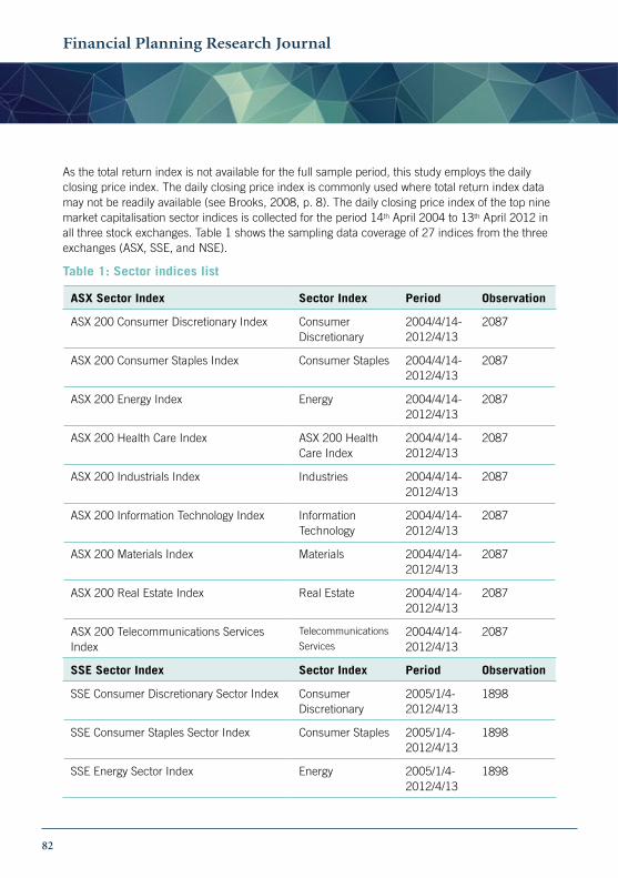
As the total return index is not available for the full sample period, this study employs the daily closing price index. The daily closing price index is commonly used where total return index data may not be readily available (see Brooks, 2008, p. 8). The daily closing price index of the top nine market capitalisation sector indices is collected for the period 14th April 2004 to 13th April 2012 in all three stock exchanges. Table 1 shows the sampling data coverage of 27 indices from the three exchanges (ASX, SSE, and NSE).

Table 1: Sector indices list

ASX Sector Index Sector Index Period Observation

ASX 200 Consumer Discretionary Index Consumer Discretionary

2004/4/14-2012/4/13

2087

ASX 200 Consumer Staples Index Consumer Staples 2004/4/14-2012/4/13

2087

ASX 200 Energy Index Energy 2004/4/14-2012/4/13

2087

ASX 200 Health Care Index ASX 200 Health Care Index

2004/4/14-2012/4/13

2087

ASX 200 Industrials Index Industries 2004/4/14-2012/4/13

2087

ASX 200 Information Technology Index Information Technology

2004/4/14-2012/4/13

2087

ASX 200 Materials Index Materials 2004/4/14-2012/4/13

2087

ASX 200 Real Estate Index Real Estate 2004/4/14-2012/4/13

2087

ASX 200 Telecommunications Services Index

Telecommunications

Services2004/4/14-2012/4/13

2087

SSE Sector Index Sector Index Period Observation

SSE Consumer Discretionary Sector Index Consumer Discretionary

2005/1/4-2012/4/13

1898

SSE Consumer Staples Sector Index Consumer Staples 2005/1/4-2012/4/13

1898

SSE Energy Sector Index Energy 2005/1/4-2012/4/13

1898


VOLUME 1. ISSUE 1

83

SSE Sector Index Sector Index Period Observation

SSE Financials Sector Index Financials 2005/1/4-2012/4/13

1898

SSE Health Care Sector Index Health Care 2005/1/4-2012/4/13

1898

SSE Industrials Sector Index Industrials 2005/1/4-2012/4/13

1898

SSE Materials Index Materials 2005/1/4-2012/4/13

1898

SSE Telecommunications Services Sector Index

Telecommunications

Services2005/1/4-2012/4/13

1898

SSE Utilities Sector Index Utilities 2005/1/4-2012/4/13

1898

NSE Sector Index Sector Index Period Observation

CNX Automobile Sector Index Automobile 2004/4/14-2012/4/13

2087

CNX Banking Sector Index Banking 2004/4/14-2012/4/13

2087

CNX Energy Sector Index Energy 2004/4/14-2012/4/13

2087

CNX Financial Sector Index Financial 2004/4/14-2012/4/13

2087

CNX Fast Moving Consumer Goods Sector Index

Fast Moving Consumer Goods

2004/4/14-2012/4/13

2087

CNX Information Technology Sector Index Information Technology

2004/4/14-2012/4/13

2087

CNX Midea Sector Midea 2004/4/14-2012/4/13

2087

CNX Metal Sector Metal 2004/4/14-2012/4/13

2087

CNX Pharmaceuticals Sector Index Pharmaceuticals 2004/4/14-2012/4/13

2087

Table 1 continued

84


VOLUME 1. ISSUE 1

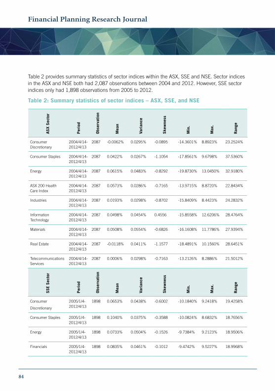
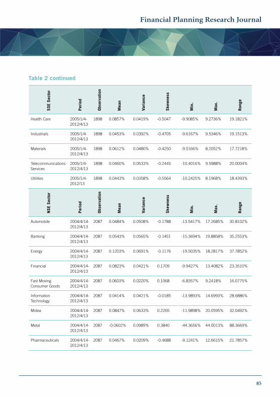
Table 2 provides summary statistics of sector indices within the ASX, SSE and NSE. Sector indices in the ASX and NSE both had 2,087 observations between 2004 and 2012. However, SSE sector indices only had 1,898 observations from 2005 to 2012.

Table 2: Summary statistics of sector indices – ASX, SSE, and NSE

AS

X S

ecto

r

Per

iod

Obs

erva

tion

Mea

n

Vari

ance

Ske

wne

ss

Min

.

Max

.

Ran

ge

Consumer Discretionary

2004/4/14-2012/4/13

2087 -0.0062% 0.0295% -0.0895 -14.3601% 8.8923% 23.2524%

Consumer Staples 2004/4/14-2012/4/13

2087 0.0422% 0.0267% -1.1054 -17.8561% 9.6798% 37.5360%

Energy 2004/4/14-2012/4/13

2087 0.0615% 0.0483% -0.8292 -19.8730% 13.0450% 32.9180%

ASX 200 Health Care Index

2004/4/14-2012/4/13

2087 0.0573% 0.0286% -0.7165 -13.9715% 8.8720% 22.8434%

Industries 2004/4/14-2012/4/13

2087 0.0193% 0.0298% -0.8702 -15.8409% 8.4423% 24.2832%

Information Technology

2004/4/14-2012/4/13

2087 0.0498% 0.0454% 0.4556 -15.8558% 12.6206% 28.4764%

Materials 2004/4/14-2012/4/13

2087 0.0508% 0.0554% -0.6826 -16.1608% 11.7786% 27.9394%

Real Estate 2004/4/14-2012/4/13

2087 -0.0118% 0.0411% -1.1577 -18.4891% 10.1560% 28.6451%

Telecommunications Services

2004/4/14-2012/4/13

2087 0.0006% 0.0298% -0.7163 -13.2126% 8.2886% 21.5012%

SS

E S

ecto

r

Per

iod

Obs

erva

tion

Mea

n

Vari

ance

Ske

wne

ss

Min

.

Max

.

Ran

ge

Consumer

Discretionary

2005/1/4-2012/4/13

1898 0.0653% 0.0438% -0.6002 -10.1840% 9.2418% 19.4258%

Consumer Staples 2005/1/4-2012/4/13

1898 0.1040% 0.0375% -0.3588 -10.0824% 8.6832% 18.7656%

Energy 2005/1/4-2012/4/13

1898 0.0733% 0.0504% -0.1526 -9.7384% 9.2123% 18.9506%

Financials 2005/1/4-2012/4/13

1898 0.0835% 0.0461% -0.1012 -9.4742% 9.5227% 18.9968%


VOLUME 1. ISSUE 1

85

SS

E S

ecto

r

Per

iod

Obs

erva

tion

Mea

n

Vari

ance

Ske

wne

ss

Min

.

Max

.

Ran

ge

Health Care 2005/1/4-2012/4/13

1898 0.0857% 0.0419% -0.5047 -9.9085% 9.2736% 19.1821%

Industrials 2005/1/4-2012/4/13

1898 0.0453% 0.0392% -0.4705 -9.6167% 9.5346% 19.1513%

Materials 2005/1/4-2012/4/13

1898 0.0612% 0.0480% -0.4250 -9.5166% 8.2052% 17.7218%

Telecommunications Services

2005/1/4-2012/4/13

1898 0.0460% 0.0533% -0.2445 -10.4016% 9.5988% 20.0004%

Utilities 2005/1/4-2012/13

1898 0.0443% 0.0358% -0.5564 -10.2425% 8.1968% 18.4393%

NS

E S

ecto

r

Per

iod

Obs

erva

tion

Mea

n

Vari

ance

Ske

wne

ss

Min

.

Max

.

Ran

ge

Automobile 2004/4/14-2012/4/13

2087 0.0484% 0.0508% -0.1788 -13.5417% 17.2685% 30.8102%

Banking 2004/4/14-2012/4/13

2087 0.0543% 0.0565% -0.1451 -15.3694% 19.8858% 35.2553%

Energy 2004/4/14-2012/4/13

2087 0.1203% 0.0691% -0.1176 -19.5035% 18.2817% 37.7852%

Financial 2004/4/14-2012/4/13

2087 0.0823% 0.0421% 0.1709 -9.9427% 13.4082% 23.3510%

Fast Moving Consumer Goods

2004/4/14-2012/4/13

2087 0.0603% 0.0220% 0.1068 -6.8357% 9.2418% 16.0775%

Information Technology

2004/4/14-2012/4/13

2087 0.0414% 0.0421% -0.0185 -13.9893% 14.6993% 28.6886%

Midea 2004/4/14-2012/4/13

2087 0.0847% 0.0633% 0.2265 -11.9898% 20.0595% 32.0492%

Metal 2004/4/14-2012/4/13

2087 -0.0602% 0.0989% 0.3840 -44.3656% 44.0013% 88.3669%

Pharmaceuticals 2004/4/14-2012/4/13

2087 0.0467% 0.0209% -0.4688 -9.1241% 12.6615% 21.7857%

Table 2 continued

86


VOLUME 1. ISSUE 1

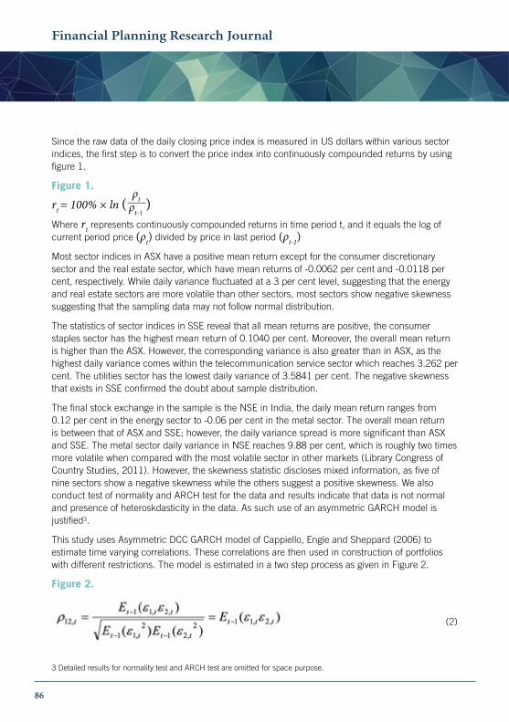
Since the raw data of the daily closing price index is measured in US dollars within various sector indices, the first step is to convert the price index into continuously compounded returns by using figure 1.

Figure 1.

rt = 100% × ln ( ρt )

Where rt represents continuously compounded returns in time period t, and it equals the log of current period price (ρt) divided by price in last period (ρt-1)Most sector indices in ASX have a positive mean return except for the consumer discretionary sector and the real estate sector, which have mean returns of -0.0062 per cent and -0.0118 per cent, respectively. While daily variance fluctuated at a 3 per cent level, suggesting that the energy and real estate sectors are more volatile than other sectors, most sectors show negative skewness suggesting that the sampling data may not follow normal distribution.

The statistics of sector indices in SSE reveal that all mean returns are positive, the consumer staples sector has the highest mean return of 0.1040 per cent. Moreover, the overall mean return is higher than the ASX. However, the corresponding variance is also greater than in ASX, as the highest daily variance comes within the telecommunication service sector which reaches 3.262 per cent. The utilities sector has the lowest daily variance of 3.5841 per cent. The negative skewness that exists in SSE confirmed the doubt about sample distribution.

The final stock exchange in the sample is the NSE in India, the daily mean return ranges from 0.12 per cent in the energy sector to -0.06 per cent in the metal sector. The overall mean return is between that of ASX and SSE; however, the daily variance spread is more significant than ASX and SSE. The metal sector daily variance in NSE reaches 9.88 per cent, which is roughly two times more volatile when compared with the most volatile sector in other markets (Library Congress of Country Studies, 2011). However, the skewness statistic discloses mixed information, as five of nine sectors show a negative skewness while the others suggest a positive skewness. We also conduct test of normality and ARCH test for the data and results indicate that data is not normal and presence of heteroskdasticity in the data. As such use of an asymmetric GARCH model is justified3.

This study uses Asymmetric DCC GARCH model of Cappiello, Engle and Sheppard (2006) to estimate time varying correlations. These correlations are then used in construction of portfolios with different restrictions. The model is estimated in a two step process as given in Figure 2.

Figure 2.

(2)

3 Detailed results for normality test and ARCH test are omitted for space purpose.

ρt-1


VOLUME 1. ISSUE 1

87

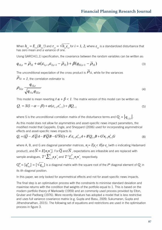
When hi,t = Et-1(R1,t2) and ri,t = √ hi,tεi,t for i = 1, 2, where εi,t is a standardized disturbance that

has zero mean and a variance of one.

Using GARCH(1,1) specification, the covariance between the random variables can be written as:

(3)

The unconditional expectation of the cross product is , while for the variances

= 1, the correlation estimator is:

(4)

This model is mean reverting if α + β < 1. The matrix version of this model can be written as:

(5)

where S is the unconditional correlation matrix of the disturbance terms and Qt = |q1,2,t|. As this model does not allow for asymmetries and asset-specific news impact parameters, the modified model that Cappiello, Engle, and Sheppard (2006) used for incorporating asymmetrical effects and asset-specific news impacts is:

(8)

where A, B, and G are diagonal parameter matrices, nt= I[εt< 0]o εt (with o indicating Hadamard

product), and N = E[ntn't]. For Q and N , expectations are infeasible and are replaced with

sample analogues, T-1∑Tt=1εtε't and T-1∑T

t=1ntn't respectively.

Q✳t = [q✳

ii,t] = [√qii,t] is a diagonal matrix with the square root of the ith diagonal element of Qt in

its ith diagonal position.

In this paper, we only looked for asymmetrical effects and not for asset-specific news impacts.

The final step is an optimisation process with the constraints to minimise standard deviation and maximise returns with the condition that weights of the portfolio equal to 1. This is based on the modern portfolio theory of Markowitz (1959) and an commonly used process provided by Elton, Gruber and Padberg (1976). More recently literature has adopted a model that is less restrictive and uses full variance covariance matrix (e.g. Gupta and Basu, 2009; Sukumaran, Gupta and Jithendranathan, 2015). The following set of equations and restrictions are used in the optimisation process in figure 3.

88


VOLUME 1. ISSUE 1

Figure 3.

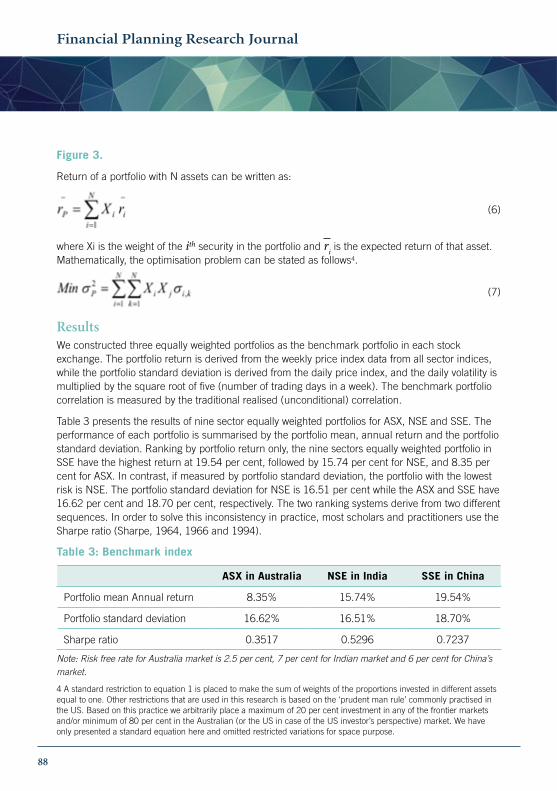
Return of a portfolio with N assets can be written as:

(6)

where Xi is the weight of the ith security in the portfolio and ri is the expected return of that asset. Mathematically, the optimisation problem can be stated as follows4.

(7)

ResultsWe constructed three equally weighted portfolios as the benchmark portfolio in each stock exchange. The portfolio return is derived from the weekly price index data from all sector indices, while the portfolio standard deviation is derived from the daily price index, and the daily volatility is multiplied by the square root of five (number of trading days in a week). The benchmark portfolio correlation is measured by the traditional realised (unconditional) correlation.

Table 3 presents the results of nine sector equally weighted portfolios for ASX, NSE and SSE. The performance of each portfolio is summarised by the portfolio mean, annual return and the portfolio standard deviation. Ranking by portfolio return only, the nine sectors equally weighted portfolio in SSE have the highest return at 19.54 per cent, followed by 15.74 per cent for NSE, and 8.35 per cent for ASX. In contrast, if measured by portfolio standard deviation, the portfolio with the lowest risk is NSE. The portfolio standard deviation for NSE is 16.51 per cent while the ASX and SSE have 16.62 per cent and 18.70 per cent, respectively. The two ranking systems derive from two different sequences. In order to solve this inconsistency in practice, most scholars and practitioners use the Sharpe ratio (Sharpe, 1964, 1966 and 1994).

Table 3: Benchmark index

ASX in Australia NSE in India SSE in China

Portfolio mean Annual return 8.35% 15.74% 19.54%

Portfolio standard deviation 16.62% 16.51% 18.70%

Sharpe ratio 0.3517 0.5296 0.7237

Note: Risk free rate for Australia market is 2.5 per cent, 7 per cent for Indian market and 6 per cent for China’s market.

4 A standard restriction to equation 1 is placed to make the sum of weights of the proportions invested in different assets equal to one. Other restrictions that are used in this research is based on the ‘prudent man rule’ commonly practised in the US. Based on this practice we arbitrarily place a maximum of 20 per cent investment in any of the frontier markets and/or minimum of 80 per cent in the Australian (or the US in case of the US investor’s perspective) market. We have only presented a standard equation here and omitted restricted variations for space purpose.


VOLUME 1. ISSUE 1

89

In this study, the risk free rate is chosen as the interbank offer rate in each country, which is 2.5 per cent, 7 per cent, and 6 per cent in Australia, India, and China respectively. When Ranking by Sharpe ratio, the nine sectors equally weighted portfolio in China had the highest Sharpe ratio at 0.72, which means an investor would receive a 0.72 per cent return by bearing one unit of risk. India ranks second with a Sharpe ratio of 0.52, and ASX ranks last with a Sharpe ratio of 0.35.

Our study uses an asymmetric DCC GARCH model to estimate the conditional correlation. We also constructed a new portfolio based on the conditional correlation with the identical sector indices within an identical time period and then compared the portfolio return with a benchmark portfolio – the nine sectors equally weighted portfolio in each stock exchange. Since the only difference between the new portfolio and the benchmark portfolio is the choice of correlation, the difference of portfolio performance will be directly contributed to the difference in correlation.

In order to simulate the real world situation when making the portfolio5, this study has two sets of restrictions, which are short sell restriction and maximum investment weight restriction for a single sector index. We restrict short selling for a number of reasons, such as; short selling may not be effective in emerging markets due to maturity of the markets and are at times banned by regulators in some countries. Regulators believe that short selling increases the volatility in the market and potentially increases speculative behaviour as borrowing an asset is less costly than actually holding it before the due date (China Securities Regulatory Commission, 2014). Maximum weighted restriction in a single asset is also a pervasive rule in the real world, such as in pension funds and those protective funds that focuses on long-term sustainable growth. This is because those kind of investments have a high level of risk aversion and putting too much weight in a single asset increases the exposure to single asset volatility.

In order to compare which correlation measurement has a better ability to capture co-movement between various sector indices, this study has constructed seven portfolios based on conditional correlation from each of the three stock exchanges. The first portfolio constructed based on conditional correlation is also an equally weighted nine sector indices portfolio, and the portfolio return is the same as the benchmark portfolio. However, the portfolio standard deviation is different from the benchmark portfolio. Therefore, the difference in the standard deviation contributes to the difference in the portfolio Sharpe ratio.

The remaining six portfolios were constructed with the combination of short sell restriction and maximum weighted restriction in the single sector index. The detailed combination are no short sell with no restriction, maximum 50 per cent weight, and maximum 20 per cent weight in the single sector index, as well as allowing 100 per cent short sell with no restriction, maximum 50 per cent weight, and maximum 20 per cent weight in the single sector index. After setting up the restrictions, the optimal portfolio is calculated based on maximising Sharpe ratio.

Table 4 states the optimal portfolio weight in each sector index, the portfolio return, portfolio standard deviation, and the Sharpe ratio in ASX. The benchmark, equally weighted nine sector portfolio in ASX had 16.62 per cent portfolio standard deviation and Sharpe ratio of 0.35.

5 These arbitrary restrictions are a common practice in the US and are referred to as ‘prudent man’s rule’; see Gupta and Donleavy (2009).

90


VOLUME 1. ISSUE 1

Table 4: ASX portfolio with different investment restrictions based on asymmetric DCC GARCH model estimated correlations.

Con

sum

er

Dis

cret

iona

ry

Con

sum

er S

tapl

es

Ener

gy

Hea

lth

Car

e In

dex

Indu

stri

es

Info

rmat

ion

Tech

nolo

gy

Mat

eria

ls

Rea

l Es

tate

Tele

com

mun

icat

ions

S

ervi

ces

Opt

imal

Por

tfol

io

Ret

urn

Por

tfol

io S

tand

ard

Dev

iati

on

Sha

rpe

Rat

io

Investment weights (Equally weighted)

11.11 %

11.11 %

11.11 %

11.11 %

11.11 %

11.11 %

11.11 %

11.11 %

11.11 %

8.35 %

16.57 %

0.3528

Investment weights (no short sell)

0.00 %

0.00 %

30.56 %

54.72 %

0.00 %

5.76 %

8.96 %

0.00 %

0.00 %

16.48 %

14.76 %

0.9474

Investment weights (no short sell with max 50% in one sector)

0.00 %

0.00 %

32.15 %

50.00 %

0.00 %

7.81 %

10.04 %

0.00 %

0.00 %

16.43 %

14.70 %

0.9475


0.00 %

0.00 %

20.00 %

20.00 %

20.00 %

20.00 %

20.00 %

0.00 %

0.00 %

13.57 %

13.72 %

0.8069

Investment weights (100% short sale)

-4.98 %

-10.89 %

50.75 %

49.93 %

49.75 %

-5.65 %

28.46 %

-50.08 %

-7.29 %

43.40 %

21.66 %

1.8883

Investment weights (100% short sale with max 50% in one sector)

-4.47

%

-10.90

%

50.00

%

49.82

%

49.78

%

-5.59

%

28.42

%

-49.93

%

-7.13

%

33.38

%

18.27

%1.8270


20.00

%

20.00

%

20.0

%

20.00

%

20.00

%

20.00

%

20.00

%

-60.00

%

20.00

%

23.24

%

16.46

%1.4119

Note: Risk free rate equal to 2.5 per cent (overnight cash rate from Reserve Bank of Australia).


VOLUME 1. ISSUE 1

91

The new equally weighted portfolio based on conditional correlation has a lower portfolio standard deviation of 16.57 per cent and Sharpe ratio of 0.35. It suggests that the conditional correlation has a higher sector diversification benefit, as the new portfolio with the same weight, same sector, and same period has a lower portfolio standard deviation.

In ASX, for the no short sell portfolio group, the portfolio risk, portfolio standard deviation, and Sharpe ratio are similar despite the weight restrictions. The Sharpe ratio decreases from 0.94 to 0.80 with 20 per cent maximum weight in one sector. As for the 100 per cent short sell portfolio group, the portfolio with no restriction has the highest Sharpe ratio of 1.88. Portfolios with restriction of maximum weight of 50 per cent and 20 per cent in one sector is has Sharpe ratios of 1.82 and 1.41 respectively.

The performance of ASX portfolios constructed using the asymmetric DCC GARCH model estimated conditional correlation significantly exceed the benchmark, as the Sharpe ratio varies from 0.35 to 1.88. The highest Sharpe ratio comes with 100 per cent short sell with no restrictions in a single asset. It is therefore not surprising, that both portfolio return and portfolio standard deviation increase significantly. The increase in returns exceeds the increase in standard deviation, which ultimately contributes to the growth of the Sharpe ratio. Other findings include that the Sharpe ratio of a portfolio, that allows 100 per cent short selling exceeds the Sharpe ratio of the portfolio that does not allow any short selling.

Table 5 illustrates the optimal portfolio weight with the portfolio return, standard deviation, and a Sharpe ratio of portfolio constructed using conditional correlations in NSE. The new equally weighted portfolio has a portfolio standard deviation of 13.6 per cent with a Sharpe ratio of 0.6428. In comparison, the benchmark portfolio has a portfolio standard deviation of 16.51 per cent with a Sharpe ratio of 0.5296. There is a decrease in portfolio risk without sacrificing portfolio returns. The Sharpe ratio of the portfolio with no short selling and with maximum 50 per cent in one single sector is 1.3678. Results for portfolios with 20 per cent maximum restrictions are also comparable. After allowing 100 per cent short selling, the portfolio Sharpe ratio increases substantially compared with the benchmark portfolio.

92


VOLUME 1. ISSUE 1

Table 5: NSE portfolio with different investment restrictions based on asymmetric DCC GARCH model estimated correlations.

Aut

omob

ile

Ban

king

Ener

gy

Fina

ncia

l

Fast

Mov

ing

Con

sum

er G

oods

Info

rmat

ion

Tech

nolo

gy

Mid

ea

Met

al

Pha

rmac

euti

cals

Opt

imal

Por

tfol

io

Ret

urn

Por

tfol

io S

tand

ard

Dev

iati

on

Sha

rpe

Rat

io


11.11 %

11.11 %

11.11 %

11.11 %

11.11 %

11.11 %

11.11 %

11.11 %

11.11 %

15.74 %

13.60 %

0.6428


0.00 %

0.00 %

39.86 %

28.82 %

14.48 %

0.00 %

16.83 %

0.00 %

0.00 %

28.34 %

15.61 %

1.3678


0.00 %

0.00 %

39.86 %

28.82 %

14.48 %

0.00 %

16.83 %

0.00 %

0.00 %

28.34 %

15.61 %

1.3678


0.00 %

0.00 %

20.00 %

20.00 %

20.00 %

0.00 %

20.00 %

0.00 %

2.00 %

23.21 %

12.70 %

1.2492


-9.15 %

-5.89 %

50.28 %

49.87 %

49.87 %

-5.80 %

28.53 %

-50.36 %

-7.33 %

49.81 %

23.11 %

1.8526


-9.12 %

-5.90 %

50.00 %

49.76 %

49.90 %

-5.74 %

28.49 %

-50.22 %

-7.18 %

49.69 %

23.04 %

1.8526


9.58 %

8.95 %

20.00 %

20.00 %

20.00 %

14.68 %

20.00 %

-33.21 %

20.00 %

32.39 %

16.00 %

1.5872

Note: Risk free rate equal to 7 per cent (overnight cash rate from Reserve Bank of India).


VOLUME 1. ISSUE 1

93

All portfolios constructed based on conditional correlation significantly outperformed the benchmark portfolio. Interestingly one pair of portfolios in the no short selling group has Sharpe ratio of 1.3678. Another pair of portfolios in the short selling group has identical Sharpe ratio of 1.8526. The identical Sharpe ratio comes from the highly similar portfolio weight, as no one sector weights over 50 per cent in the portfolio. Moreover, the Sharpe ratio of all portfolios, using NSE indices, allowing for 100 per cent short selling outperform the portfolio that does not allow short selling.

Table 6 shows the optimal portfolio weight with portfolio return, portfolio standard deviation, and Sharpe ratio in SSE. The new equally weighted portfolio also outperforms the benchmark, as the new equally weighted portfolio Sharpe ratio equals 0.9213 compared with the benchmark portfolio that has a Sharpe ratio of 0.7232.

The Sharpe ratio of the no short selling portfolio group is 1.4080, 1.3968, and 1.1776 with no restriction in weight, maximum 50 per cent weight, and maximum 20 per cent weight in a single sector respectively. The 100 per cent short selling portfolio group also outperforms the benchmark, the highest portfolio Sharpe ratio comes with 100 per cent short selling with no restriction in weight. However, the magnitude of the outperformance is relatively small when compared with the Australian and Indian markets.

Table 6: SSE portfolio with different investment restrictions based on asymmetric DCC GARCH model estimated correlations

Con

sum

er

Dis

cret

iona

ry

Con

sum

er S

tapl

es

Ener

gy

Fina

ncia

ls

Hea

lth

Car

e

Indu

stri

als

Mat

eria

ls

Tele

com

mun

icat

ions

S

ervi

ce

Uti

liti

es

Opt

imal

Por

tfol

io

Ret

urn

Por

tfol

io S

tand

ard

Dev

iati

on

Sha

rpe

Rat

io


11.11 %

11.11 %

11.11 %

11.11 %

11.11 %

11.11 %

11.11 %

11.11 %

11.11 %

19.54 %

14.69 %

0.9213


0.00 %

63.13% 0.00%25.21

%11.66

%0.00 %

0.00 %

0.00 %

0.00 %

28.87 %

16.24 %

1.4080


0.00 %

50.00 %

0.00 %

29.43 %

20.57 %

0.00 %

0.00 %

0.00 %

0.00 %

28.03 %

15.77 %

1.3968

94


VOLUME 1. ISSUE 1

Con

sum

er

Dis

cret

iona

ry

Con

sum

er S

tapl

es

Ener

gy

Fina

ncia

ls

Hea

lth

Car

e

Indu

stri

als

Mat

eria

ls

Tele

com

mun

icat

ions

S

ervi

ce

Uti

liti

es

Opt

imal

Por

tfol

io

Ret

urn

Por

tfol

io S

tand

ard

Dev

iati

on

Sha

rpe

Rat

io


13.97 %

20.00 %

20.00 %

20.00 %

20.00 %

0.00 %

5.69 %

0.00 %

0.52 %

24.05 %

16.32 %

1.1776


-7.23 %

97.01 %

14.56 %

42.33 %

28.59 %

-28.70 %

-10.53 %

-18.09 %

-17.96 %

39.69 %

21.84 %

1.5430


-1.87 %

50.00 %

14.78 %

41.74 %

38.12 %

-15.09 %

-4.86 %

-12.50 %

-10.33 %

32.62 %

18.11 %

1.4697


17.98 %

20.00 %

20.00 %

20.00 %

20.00 %

-7.55 %

8.87 %

-3.83 %

4.53 %

24.43 %

15.58 %

1.1831

Note: Risk free rate equal to 6 per cent (overnight cash rate from People’s Bank of China).

In order to increase the robustness of the findings, this study employs an out of sample test with a two-year time period from 14th April 2012 to 14th April 2014 containing 522 observations, following the sampling period from 14th April 2002 to 13th April 2012.

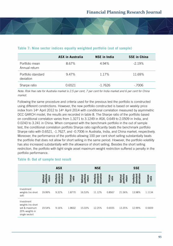
Table 7 shows the new nine sector indices equally weighted benchmark portfolio. The Sharpe ratio for the three benchmark portfolios are 0.6521, -1.7627, and -0.7006 in Australia, India, and China, respectively. The negative Sharpe ratios of the benchmark portfolios in India and China suggest that the return on the portfolio is less than the return of the risk-free investment. However, it is rare to see any benchmark portfolios generate a negative Sharpe ratio in the real world, as the investor has the flexibility to shift from the stock market to the bond market if the stock market shows an unfavourable trend (Strong, 2009). Since the available assets have been restricted to the stock market only in this study, the negative Sharpe ratio is accepted as a baseline to test the sector diversification performance.

Table 6 continued


VOLUME 1. ISSUE 1

95

Table 7: Nine sector indices equally weighted portfolio (out of sample)

ASX in Australia NSE in India SSE in China

Portfolio mean Annual return

8.67% 4.94% -2.19%

Portfolio standard deviation

9.47% 1.17% 11.69%

Sharpe ratio 0.6521 -1.7626 -.7006

Note: Risk free rate for Australia market is 2.5 per cent, 7 per cent for India market and 6 per cent for China market.

Following the same procedure and criteria used for the previous test the portfolio is constructed using different constrictions. However, the new portfolio constructed is based on weekly price index from 14th April 2012 to 14th April 2014 with conditional correlation measured by asymmetric DCC GARCH model, the results are recorded in table 8. The Sharpe ratio of the portfolio based on conditional correlation varies from 1.3271 to 3.1249 in ASX, 0.649 to 2.0509 in India, and 0.0243 to 3.241 in China. When compared with the benchmark portfolio in the out of sample test, the conditional correlation portfolio Sharpe ratio significantly beats the benchmark portfolio Sharpe ratio with 0.6521, -1.7627, and -0.7006 in Australia, India, and China market, respectively. Moreover, the performance of the portfolio allowing 100 per cent short selling substantially beats the portfolio that does not allow for short selling in the same period. However, the portfolio volatility has also increased substantially with the allowance of short selling. Besides the short selling restriction, the portfolio with tight single asset maximum weight restriction suffered a penalty in the portfolio performance.

Table 8: Out of sample test result

ASX NSE SSE

Opt

imal

po

rtfo

lio

retu

rn

Por

tfol

io

stan

dard

de

viat

ion

Sha

rpe

rati

o

Opt

imal

po

rtfo

lio

retu

rn

Por

tfol

io

stan

dard

de

viat

ion

Sha

rpe

rati

o

Opt

imal

po

rtfo

lio

retu

rn

Por

tfol

io

stan

dard

de

viat

ion

Sha

rpe

rati

o


19.99% 9.32% 1.8770 16.53% 11.12% 0.8567 21.56% 13.98% 1.1134

Investment weights (no short sell & maximum 20% weights in single sector)

19.54% 9.16% 1.8602 15.03% 12.25% 0.6555 13.35% 12.99% 0.5659

96


VOLUME 1. ISSUE 1

ASX NSE SSE

Opt

imal

po

rtfo

lio

retu

rn

Por

tfol

io

stan

dard

de

viat

ion

Sha

rpe

rati

o

Opt

imal

po

rtfo

lio

retu

rn

Por

tfol

io

stan

dard

de

viat

ion

Sha

rpe

rati

o

Opt

imal

po

rtfo

lio

retu

rn

Por

tfol

io

stan

dard

de

viat

ion

Sha

rpe

rati

o

Investment weights (no short sell & maximum 50% weights in single sector)

15.32% 9.66% 1.3271 13.53% 10.05% 0.6490 6.28% 11.68% 0.0243

Investment weights (maximum 100% short sell)

84.71% 26.31% 3.1249 79.67% 35.43% 2.0509 95.49% 27.61% 3.2411

Investment weights (maximum 100% short sell & maximum 20% weights in single sector)

48.57% 17.17% 2.6823 51.09% 24.24% 1.8184 54.80% 19.10% 2.5579

Investment weights (maximum 100% short sell & maximum 50% weights in single sector)

21.35% 10.40% 1.8119 20.80% 17.08% 0.8083 12.22% 12.22% 0.9052

Note: Risk free rate for Australia market is 2.5 per cent, 7 per cent for India market and 6 per cent for China market.

The portfolio constructed based on conditional correlation significantly beats the benchmark portfolio, which is highly consistent with the previous test performed on the 2004 to 2012 data, which suggests the model is robust.

Conclusion

This study looks at the sector diversification benefits across three markets that includes two significantly large emerging markets and one developed market. Findings using a computationally efficient and theoretically sound ADCC GARCH model suggest that there can be gains in diversifying portfolios across sectors in emerging and developed markets. Results of the study are robust and the findings can be used for practical benefits when investing.

Table 8 continued


VOLUME 1. ISSUE 1

97

The results of the portfolio constructed with conditional correlation measured by the asymmetric DCC GARCH model significantly outperforms the benchmark portfolio constructed in the traditional correlation matrix, revealing that the asymmetric DCC GARCH model is a feasible and superior model to measure the conditional correlation regardless of political background and market structure. This finding is significant as three crucial factors that influence portfolio construction are returns, riskiness, and correlation. Since all three factors are decided by the market, the better measurement of any one of the three factors will make a positive contribution for all investors. As a result, use of a theoretically sound model provides better estimation of inputs in portfolio construction. The model is computationally efficient and can easily be used in portfolio construction by investotrs and fund managers.

Furthermore, the simulation of real world market restrictions also provides practical relevance of the study. Results of unconstrained portfolios are superior to the constrained portfolios. However, in the real world, investors are less likely to heavily short sell a particular sector. Additionally, short selling is restricted (or not available) in emerging markets. As such, the application of these restrictions provide more meaningful findings for practitioners.

The main contribution to the existing literature is extending the sector diversification studies with an asymmetric DCC GARCH model into the China stock market. China, as a leading developing country in emerging markets with unique political and economic structure is relatively under-researched. The results from this study show that the benefits of sector diversification in China are similar to the other emerging markets and developed marketsdespite unique economic structures in China (People’s Daily, 2000).

One of the limitations of this study is the insufficient data source, which is pervasive for studies focusing on emerging markets, particularly because the Shenzhen Stock Exchange (SZSE) cannot provide sufficient observation data to perform the asymmetric DCC GARCH model correlation estimate. Despite these limitations, the data available was sufficient for the research question in the study and appropriate conclusions can be made with the available data.

98


VOLUME 1. ISSUE 1

References

Baumöhl, E. and Lyócsa, Š. (2014) ‘Volatility and dynamic conditional correlation of worldwide emerging and frontier markets’, Economic Modeling, 38, pp. 175-183.

Beine, M. and Coulombe, S. (2007) Economic integration and the diversification of regional exports: evidence from the Canadian–U.S. Free Trade Agreement’, Journal of Economic Geography, 7, pp. 93–111.

Brooks, C. (2008) Introductory Econometrics for Finance (2nd ED), UK: Cambridge university press.

Cappiello, L., Engle, R. F. and Sheppard, K. (2006) ‘Asymmetric Dynamics in the Correlations of Global Equity and Bond Returns’, Journal of Financial Econometrics, 4, pp. 537-572.

Cheng, C. (2001) Sector Diversification, Morningstar, http://www.hk.morningstar.com/HKG/ARTICLES/FEATUREARTICLE.ASP?ArticleId=%2FODS%2F2000%2FFATT%2F2000FATT164E_20010713.XML&change_needed=EN

China Securities Regulatory Commission. (2014) Monthly security market statistics, Viewed at http://www.csrc.gov.cn/pub/newsite/sjtj/zqscyb/index_6.html.

Clark, E. and Tunaru, R (2001) ‘Emerging markets: Investing with political risk’, Multinational Finance Journal, 5:3, pp 155-173.

Dunis, C. L. and Shannon, G. (2005) ‘Emerging markets of South-East and Central Asia: Do they still offer a diversification benefit?’, Journal of Asset Management, pp. 168-190.

Elton, E. J, Gruber, M. J and Padberg, M. W. (1976) ‘Simple Criteria for Optimal Portfolio Selection’, Journal of Finance, 31:5, pp. 1341-1357.

Engle, R. (1982) ‘Autoregressive Conditional Heteroscedasticity with Estimates of the Variance of United Kingdom Inflation’, Econometrica, 50, pp. 987-1007.

Errunza, V. R. (1983) ‘Emerging Markets: A New Opportunity For Improving Global Portfolio Performance’, Financial Analysts Journal, 39, pp. 51-58.

Forbes, K. and Rigobon, R. (2002) ‘No Contagion, Only Interdependence: Measuring Stock Market Comovements’, Journal of Finance, 57:5, pp. 2223-2261.

Godfrey, L. G. (1978) ‘Testing Against General Autoregressive and Moving Average Error Models when the Regressors Include Lagged Dependent Variables’, Econometrics, 46, pp. 1293-1302.

Gupta, R. and Basu, P. K. (2011) ‘Does Sector Diversification Benefit All Markets?- Anaylsis of Australia and Indian Markets’, Asia Pacific Journal of Economic & Business, 15, pp. 15-25.


VOLUME 1. ISSUE 1

99

Gupta, R. and Donleavy, G.D. (2009) ‘Benefits of diversifying investments into emerging markets with time-varying correlations: An Australian perspective’, Journal of Multinational Financial Management, 19:2, pp. 160-177.

Hargis, K. and Mei, J. (2006) ‘Is Country Diversification better than Industry Diversification?’, European Financial Management, 12, pp. 319-340.

Huang, J.-Z. and Zhong, Z. (2006) Time-variation in diversification benefits of commodity, REITs, and TIPS, 2006 China International Conference in Finance, International Monetary Fund, viewed in 2014 at http://www.imf.org/external/index.htm.

Jarque, C. M. and Bera, A .M. (1981) ‘Efficient tests for normality, homoscedasticity and serial independence of regression residuals: Monte Carlo evidence’, Economics Letters, 7, pp. 313-318.

Kohers, T. Kohers, G. and Pandey, V. (1998) ‘The contribution of emerging markets in international diversification strategies’, Applied Financial Economics, 8, pp. 445-454.

Lessard, D. R. (1976) ‘World, Country, and Industry Relationship in Equity Returns. Implications for Risk Reduction Through International Diversification’, Financial Analysts Journal, 32, pp. 32-38.

Library of Congress (2011) Library of Congress Country Studies (5th ed.) Country Profile: India, retrieved September 30, 2011, Library of Congress Federal Research Division.

Longin, F. and Solnik, B. (2001) ‘Extreme correlation of international equity markets’, Journal of Finance, 56, pp. 649–676.

Markowitz, H. (1952) ‘Portfolio selection’, Journal of Finance, 7, pp. 77-91.

Markowitz, H. (1959) Portfolio Selection: Efficient Diversification of Investment, Wiley, New York.

People’s Daily. (2000, November 15) China Committed to Open Economic Policy: President, viewed at http://english.peopledaily.com.cn/english/200011/15/eng20001115_55215.html.

Shanghai Stock Exchange. (2014) Viewed at http://english.sse.com.cn/.

Sharpe, W. F. (1964) ‘Capital asset prices: A theory of market equilibrium under conditions of risk’, Journal of Finance, 19, pp. 425-442

Sharpe, W. F. (1966) ‘Mutual Fund Performance’, Journal of Business, 39, pp. 119-138.

Sharpe, W. F. (1994) ‘The Sharpe Ratio’, Journal of Portfolio Management, 21, pp. 49-58.

Strong, R. (2009) Portfolio Construction, Management, and Protection, South-Western Cengage Learning, USA.

Sukumaran, A., Gupta, R. and Jithendranathan, T. (2015) ‘Looking at new markets for international diversification: frontier markets’, International Journal of Managerial Finance, 11:1, pp. 97-116.

100


VOLUME 1. ISSUE 1

Syllignakis, M. N. and Kouretas, G. (2011) ‘Dynamic correlation analysis of financial contagion: Evidence from the Central and Eastern European markets’, International Review of Economics & Finance, 20:4, pp. 717-732.

Whalen, C. (2008) ‘Understanding the Credit Crunch as a Minsky Moment’, Challenge, 51:1, pp. 91-109.

World Federation of Exchange. (2014) Monthly Reports, View at: http://www.world-exchanges.org/statistics/monthly-reports.

Yang, S. (2005) ‘A DCC analysis of international stock market correlations: the role of Japan on the Asian Four Tigers’, Applied Financial Economics Letter, 1, pp. 89-93.

Zhang, B., Li, X. and Yu, H. (2013) ‘Has recent financial crisis changed permanently the correlations between BRICS and developed stock markets?’, The North American Journal of Economics and Finance, 26:C, pp. 725-738.

financial planning research journal - griffith

Documents