financial reporting frequency and external finance
TRANSCRIPT

Financial reporting frequency and external finance:
Evidence from a quasi-natural experiment
Ryosuke Fujitani
PhD. Student
Graduate School of Commerce and Management,
Hitotsubashi University
August 2019
No.230

1
Financial reporting frequency and external finance:
Evidence from a quasi-natural experiment*
Ryosuke Fujitani
Graduate School of Commerce and Management, Hitotsubashi University
2-1 Naka, Kunitachi, Tokyo 186-8601, Japan
This version: August 2019
The latest version: https://papers.ssrn.com/sol3/papers.cfm?abstract_id=3410252
* Ryosuke Fujitani greatly appreciates financial support from a Grant-in-Aid for JSPS Research Fellow (No.
JP17J03278) provided by Japan’s Ministry of Education, Science, Sports, and Culture.

2
Financial reporting frequency and external finance:
Evidence from a quasi-natural experiment
Abstract: Using a unique institutional background of Japan, this study first examines the
effects of the increase in the reporting frequency on corporate financing. From Difference-
in-Difference (DiD) analysis, I show that the increase in the reporting frequency increases
external finance but not finance from bank. Next, I find that the positive effects of the
increase in the reporting frequency are stronger in firms with a) financial constraints, b)
ex-ante information asymmetry, and c) more external capital demand. I also find that the
firms a) do not change the cash holding intensity, b) invest more, and c) payout more.
Unlike prior literature, these findings suggest that the increase in the reporting frequency
enhances firm activities.
JEL Classification: G31, G32, M41
Key words: financial reporting frequency, quarterly reporting, quasi-private firms, external
finance, pecking order theory

3
1. Introduction
This study examines the effects of the financial reporting frequency on corporate
financing. Prior literature has shown that more frequent financial reporting improves the stock
market efficiency (Fu et al., 2012) and agency problems in terms of cash holding (Downer et al.,
2018), suggesting that the frequent reporting mitigates information friction. However, little
literature investigates economic consequences of the reduced cost of capital on corporate decision
making. Thus, this study sheds light on the new aspects of economic consequences of frequent
financial reporting, i.e. corporate capital funding.
Pecking order theory provides the perspective on the relation between information friction
and corporate finding. Myers (1984) and Myers and Majluf (1984) document that the information
asymmetry of insiders and outsiders of a firm increases the cost of capital of external finance
resource, suggesting that managers prefer financing from internal capital to avoid the relative
higher cost. A bulk of empirical studies provide the evidence consistent with Myers’ discussion.1
From the perspective of pecking order theory, the decline of cost of capital enhances the
ability of firms to finance from external sources. The cost of external capital can be mitigated by
mitigating the information asymmetry. Prior literature shows the negative relation between
information quality and cost of capital. Lee and Masulis (2009) show that information asymmetry
measured by lower accounting quality increases the flotation costs. Biddle and Hilary (2006) and
Balakrishnan et al. (2014) show that higher accounting quality mitigate financial constraints driven
by information friction, suggesting that accounting information decreases external finance costs.
Frequent financial reporting can mitigate the information asymmetry. AICPA (1994)
discusses that more frequent financial reporting conveys relevant information to security market
1 Myers (2003) and Frank and Goyal (2008) are good reviews.

4
participants. Consistent with this discussion, a bulk of studies find the evidence that more frequent
financial reporting provides relevant information. Fu et al. (2012) find that more frequent reporting
reduces information asymmetry and the cost of equity.
Extending these findings, I expect that the increase in financial reporting frequency
increases external finance, but not less costly capital source. Frequent financial reporting decreases
information asymmetry between insiders and outsiders, decreasing cost of external capital.
Consequently, firms can access more external finance. On the other hand, I expect that the
reporting frequency weakly or no longer relates loans and internal capital funding, since public
information might not be an important information source for bank loans. First, firms privately
negotiate the loan contract with banks. Second, when banks require firms to disclose corporate
information, firms do not necessary disclose the information publicly. For instance, Regulation FD
requires firms to convey their information through public disclosure for equity market, but not
necessarily debt market (Petacchi, 2015). Third, from pecking order perspective, the decrease in
information asymmetry substantially increase external finance, but not internal finance and bank
loans.
To test the expectation, I focus on the increase in the frequency of financial reporting in
Japan, since it gives a natural set of control firms for my Difference-in-Difference (DiD) design.
This study uses Japanese quasi-private firms (Baderscher et al., 2019). Quasi-private firms are the
firms required to disclose 10-K and semi-annual financial reporting. Stock exchanges in Japan
started requiring listed firms to report quarterly financial reporting (as Form 10-Q in the U.S.), but
not for private firms including quasi-private firms.
My DiD approach shows that the initiation of quarterly financial reporting increases
corporate external finance, but not bank loan finance. This positive effect is stronger for firms with
1) financial constraints, 2) serious information asymmetry, and 3) higher demand for external

5
finance. These results suggest that more frequent financial reporting mitigates information
problem or agency problem. I next examine how the firms use the raised capital, and show that the
frequent financial reporting increases corporate investment and payout, but not cash holding.
These findings indicate that more frequent reporting promotes corporate capital turnover.
The main contribution of this study is to nest a plausible mechanism linking financial
reporting frequency and corporate activities, especially capital raising. Financial economists have
shown the link between reporting frequency and security market efficiency. Their findings imply
that the increase in reporting frequency help firms access to external capital. Despite the
importance of the controversy, there is little evidence on the relation between the frequency of
reporting and corporate capital raising. This study complements prior literature by showing a new
evidence on the economic consequences of frequent financial reporting. Specifically, frequent
financial reporting enhances corporate external financing through mitigating external cost of
capital.
The other contribution is to shed light on the bright side of frequent financial reporting.
Several prior studies show the cost of frequent reporting: managerial short-termism. Kraft et al.
(2018) and Ernstberger et al. (2017) show that firms reduce long-term investment to increase short-
term profit. However, this study finds that, at least in Japan, frequent reporting increases corporate
external finance and enhances their activities including investment and payout. These findings are
consistent with the idea that frequent reporting conveys relevant information to security market
participants, then help firms finance external capital.
This study is organized as follows. The next section describes the institutional background
of Japanese disclosure regulation. In section 3, I describe the data, regression model and finance
measure. Section 4 represents the results of main analyses and their robustness tests. Section 5
explains the research design of additional analyses and their results. Finally, Section 6 concludes

6
this study.
2. Institutional Background
This study uses quasi-private firms as the counter factual of listed firms which are
required to report the quarterly financial statements as my research setting. Quasi-private firms are
the firms with over 1,000 shareholders or the firms issuing public security. Japanese Financial
Instrument Exchange Act mandates these firms to disclose annual and semi-annual financial
reporting (like Form 10-K and the second quarter Form 10-Q in the U.S., respectively).2 Thus, the
quasi-private firms report the same frequency and the information contents before the initiation of
quarterly financial reporting.
In 2003, Japanese stock exchanges (e.g., Tokyo Stock Exchange) mandated listed firms
the quarterly financial statements, and effective from the first quarter after April 1, 2003. In 2008,
the revised Financial Instrument Exchange Act mandated all the listed firms to report quarterly
financial reporting. However, unlisted firms, including the quasi-private firms, are not mandated
to report the quarterly financial reporting.
This difference regulatory background of semi-annual and quarterly financial reporting
offers an advantage to examine the effects of the increase in reporting frequency on corporate
financing. By comparing the quasi-private firms with the listed firms that were mandated to change
the reporting frequency, I can identify the effects of the changes in the reporting frequency and
mitigate endogeneity concerns associated with the choice of reporting frequency. The fact that the
listed and the quasi-private firms are required to publish the same frequency and level of financial
reporting prior to 2003 gives us a natural set of control firms for my DiD analysis. Figure 1
2 Please see French et al. (2019) for the institutional backgrounds of quasi-private firms in Japan.

7
describes my DiD research framework.
**Insert Figure 1 here**
3. Research Design
3.1 Sample and matching procedure
The initial sample comprises all of Japanese non-financial firms in Nikkei NEEDS
Financial QUEST (FQ) during the fiscal years (FY) 2000 March through 2009 February. FQ
contains the financial data of Japanese listed and quasi-private, and a part of data of purely-private
firms. Since I use lagged variable in my analysis, the sample contains the data from FY 2001 March
through FY 2009 February. Following prior literature (Ernstberger et al., 2017; Kraft et al., 2018),
I exclude the treatment year (FY 2004 March to FY 2005 February) from the analyses. I also
exclude from the sample firms a) following any other accounting standards than Japanese GAAP;
b) reporting 10 K containing the financial information less than 12 months or more than 12 months.
I identify the unlisted firms which do not have exchange ID (EXCHANGE in FQ code). To exclude
purely-private firms from my sample, I limit the unlisted firms reporting a) cashflow statement
and b) ownership structure, since purely-private firms do not disclose them.
Following the approach of prior literature, I identify a matched quasi-private firm for each
treatment firm as control firm that did not change reporting frequency during the treatment year. I
use caliper-based nearest neighborhood matching to identify the set of control firms. Specifically,
I limit the firms with data available in the analyses during the periods three years prior to and three
years after the treatment year. I estimate a propensity score model using firm size (size) for each
industry in the beginning FY of my test (FY 2001April to FY 2002 February) to identify a control
firm for each treatment firm. I employ nearest-neighbor matching and drop observations with
propensity scores outside the common support to ensure high match quality. Once a match is

8
formed, it is kept in subsequent years to ensure the panel structure remains intact.
The final sample consists of 2,317 firm-year observations. The number of observations is
odd since several firms drop from the sample 4 years after the treatment year. A t-test of differences
in the mean level of firm size (size) across treatment and control firms before the treatment year
does not reject the null hypothesis of equal means (|t| = 0.0096). To mitigate the effects of outliers,
I winsorize all variables at the 1st and 99th percentiles.
3.2 Financing measurements
This study uses three corporate financing measurements. Total financing (fin_tot) is the
sum of the cash inflow from loan, issues of bond, compatible bond, and stock. This measurement
represents the total corporate financing behavior. External financing (fin_ex) is the sum of the cash
inflow from issues of bond, compatible bond, and stock. This captures the corporate external
financing. Bank loan financing (fin_loan) is the increase in short- and long-term debt. All the
measures are scaled by the sum of the tangible and intangible assets. Since several firms report the
net amount of cashflow from these financing, I take net of cash inflow from each financing
resource.
3.3 Regression
My baseline regression for testing my hypothesis is as follows:
financeit = 1 post + 2 treat×post + z + fe + it
(1)
where finance is a measure of corporate financing behavior; treat is an indicator variable for
treatment firms i.e., listed firms; post is an indicator variable that equals 1 for periods after the
treatment year, and 0 for periods prior to the treatment year. The vector z represents the control
variables, which include sales growth (sg), operating cash flow (cfo), natural logarithm of lagged
total assets (size), natural logarithm of lagged firm age (age), and lagged cash holding (cash),

9
lagged leverage (lev), lagged retained earnings (retain). To mitigate the heteroskedasticity, all the
variables except sales growth, firm age and firm size are scaled by the sum of tangible and
intangible assets. The vector fe represent the time-invariant firm fixed effects. The standard errors
clustered by firm.
The variable in interest is the interaction term between the treatment indicator and the
post indicator (treat×post). The coefficient on the interaction measures the change in firm’s
financing behavior for treatment firms around the reporting frequency increases compared to
corresponding changes in financing of control firms. My main hypothesis predicts that the external
financing increases after the reporting frequency increases. Consequently, I expect that 2 > 0 in
Model (1) when the dependent variable is external finance. On the other hand, bank loans which
exhibit lower costs might not change in response to the change in reporting frequency. Thus, I
expect that 2 is statistically indistinguishable from zero, which is consistent with my expectation
(but do not support my expectation).
4. Results
4.1 Descriptive statistics and univariate analysis
Table 1 presents descriptive statistics for each of the main variables. Prior to the change
in reporting frequency, treatment firms finance more than control firms from any financing sources.
These differences increase following treatment, which support my expectation.
**Insert Table 1 here**
4.2 Frequent reporting and financing
Table 2 reports the regression results from estimates of the Model (1). In Column (1), the
dependent variable is total financing (fin_tot). The coefficient on the interaction term is positively
significant, suggesting the increase in reporting frequency increases corporate financing behavior.

10
In Column (2), the dependent variables are external financing (fin_ext). The coefficients on
interaction term are positively significant. This suggests that firms increase external financing after
initiation of quarterly financial reporting. On the other hand, Column (3) presents that loan finance
does not change following the increase in reporting frequency, suggesting that the reporting
frequency does not enhance the financing from bank.
**Insert Table 2 here**
To test the persistence of the effects of the increase in the reporting frequency, I divide
the treatment period indicator (post) into two periods (post(+1,+2) and post(+3,+4)). Column (1)
presents that the effects of the increase in financial frequency on total finance continue through
following two years. Column (2) suggests that the positive effects of frequent financial reporting
are temporary. Bank loan still does not change (Column (3)), which support the idea that firms do
not change the financing strategy from lower cost financing sources.
Next, I test the parallel trend assumption underlying my DiD estimation. The parallel
trend assumption states that both treatment and control groups would follow the parallel
movements if treatment were not initiated. Following prior literature, in Columns (7) – (9), I
include pre-treatment time period indicator variables (before(-1)) to explore whether investments
in treatment and control groups exhibit any differential changes prior to the treatment year. The
coefficients on the interaction between treatment indicator and pre-treatment time period indicator
(treat×before(-1)) are statistically insignificant. The coefficients on the treatment between
treatment indicator and post periods indicator are significantly positive for total finance and
external finance, but not significant for bank loans. These findings suggest that treatment and
control firms exhibit parallel trends in investments prior to the reporting frequency increase, but
these trends diverge only after the reporting frequency increase.
4.3 Robustness tests

11
In this section, I check the robustness of the results. First, to address the endogeneity
problem to be listed, I run the treatment effect model. The effect of treatment (being listed) might
be different across firms and could affect the probability of firms going listed. Therefore, following
Acharya and Xu (2017), I apply the treatment effect model which can adjust for the selection bias
by using the inverse Mills ratio. The treatment effect model is the two-step approach. In the first
step, I regress the treatment indicator on the determinants to go listed (Model (2)):
Pr (treatit = 1) = 0 + 1 w + it
mills := treatit (0 + 1 w) + (treatit -1) (0 + 1 w)
(2)
where w is a set of firm characteristics variables that might affect a firm’s choice to be listed. I
include log of sales, sales growth, ROA, age, and leverage. Using matched sample, the coefficients
are estimated from the probit model.
The inverse mills ratio (mills) computed from the model (4) is added to model (1) to
correct the selection bias:
financeit = 1 post + 2 treat × post + 3 mills + z + fe + it
(3)
where finance is a measure of corporate financing behavior; treat is an indicator variable for
treatment firms i.e., listed firms; post is an indicator variable that equals 1 for periods after the
treatment year, and 0 for periods prior to the treatment year. To address the endogeneity problem,
inverse mill’s ratio is included. The vector z represents the control variables, which include sales
growth (sg), operating cash flow (cfo), natural logarithm of lagged total assets (size), natural
logarithm of lagged firm age (age), and lagged cash holding (cash), lagged leverage (lev), lagged
retained earnings (retain). To mitigate the heteroskedasticity, all the variables except sales growth
and firm size are scaled by the sum of tangible and intangible assets. The vector fe represent the

12
time-invariant firm fixed effects. The standard errors clustered by firm.
The results are reported in Columns (1) – (3) of Table 3. The coefficients on the interaction
terms are positively significant in Columns (1) and (2), but not statistically significant in Column
(3). These results suggest that the main findings are robust after adjusting for the endogeneity
problem on the choice to be listed.
**Insert Table 3 here**
I further examine the robustness of my main findings by using alternative matching
procedures. I use alternative variables to match a quasi-private firm to each listed firm. In Columns
(4) – (6) in Table 3, I use industry, size, firm age, and leverage to identify a matched sample. And,
in Columns (7) – (9), I use industry, size, age, leverage, cash holding, and sales growth. The results
show that the initiation of the quarterly financial reporting increases total financing and external
financing, but not change bank loans. These results suggest that my findings are not sensitive to
matching procedures.
5. Additional tests
5.1 Heterogeneity
To specify whether my expectation can explain the increase in external financing after the
reporting frequency increases, I perform multiple additional analyses. First, I test the financing of
financial constrained firms. If financial reporting frequency mitigates financial constraints, the
effects of change in reporting frequency are stronger for firms facing more serious financial
constraints. Next, I investigate the relation between the ex-ante information asymmetry the effects
of the reporting frequency. The seriousness of financial constraints depends on information
asymmetry between insiders and outsiders. Thus, ex ante information asymmetry enhances the
effects of frequent financial reporting on external finance. Finally, I focus on external finance

13
demand. Firms with intense external capital demand face more serious financial constraints. On
the other hand, if firms have lower external capital demand and have enough internal capital with
relatively low cost, the frequent financial reporting no longer matters for these firms. Thus, I expect
that the effects of frequent financial reporting are stronger for firms with higher external finance
demand.
To examine the expectations, I regress the estimation mode as follows:
financeit = 1 post + 2 treat × post + X × treat × post + z + fe + it
(4)
where finance is a measure of corporate financing behavior; treat is treatment indicator; post is an
indicator variable that equals 1 for periods after the treatment year, and 0 for periods prior to the
treatment year. X is the variable of the factors changing the effects of treatment. I use firm size and
Hadlock-Pierce index as the proxy of financial constraints (Hadlock and Pierce, 2010; Farre-
Mensa and Ljungqvist, 2015). Amihud’s (2002) illiquidity index is uses as the proxy of ex ante
information asymmetry of firms. Firm size also proxies the seriousness of adverse selection (Frank
and Goyal, 2003). In external finance demand test, I use Rajan and Zingales’ (1997) external
capital dependence measure.
The vector z represents the control variables, which include sales growth (sg), operating
cash flow (cfo), natural logarithm of lagged total assets (size), natural logarithm of lagged firm age
(age), and lagged cash holding (cash), lagged leverage (lev), lagged retained earnings (retain). To
mitigate the heteroskedasticity, all the variables except sales growth and firm size are scaled by
the sum of tangible and intangible assets. The vector fe represent the time-invariant firm fixed
effects. The standard errors clustered by firm.
**Insert Table 4 here**
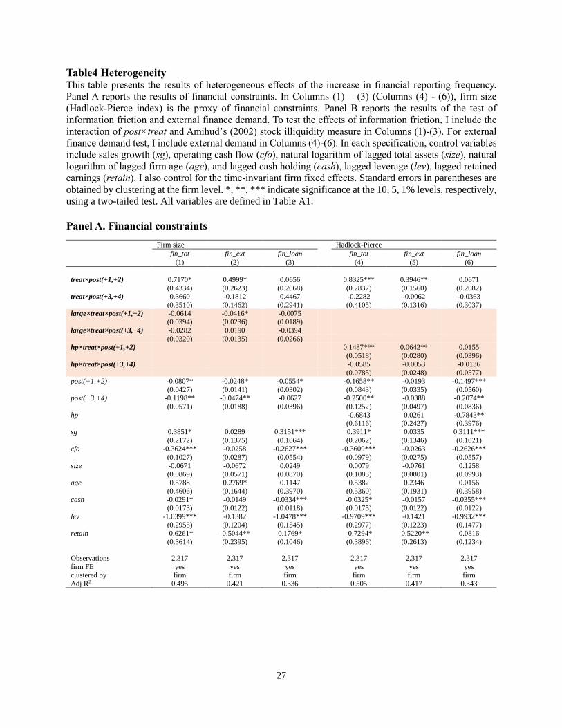
Panel A of Table 4 reports the results of Model (4). Columns (4)-(6) show the results of

14
Model (4) using Hadlock-Pierce index as the proxy of financial constraints. The coefficients on
the interaction between treatment and post indicators and Hadlock-Pierce index (treat×post×hp)
is positively significant for total finance and external finance, but not statistically significant for
bank loan. These findings suggest that the positive effects of quarterly financial reporting are
stronger for firms with more financial constraints problem. This evidence is consistent with my
expectation.
5.2 How do firms use the capital?
My main findings do not exclude another explanation that firms raise capital not to
increase firm value. For instance, if firms increase the capital and hold it as cash reserve on hand,
the financing does not enhance firm’s business activities. To examine how the firms use their raised
external capital, I examine the effects of the change in financial reporting frequency on other
aspects of corporate activities. I focus on three aspects of corporate behavior: cash holding,
investment, and payout. To test the effects, I regress the equation as follows:
activityit = 1 post + 2 treat × post + z + fe + it
(5)
where activity is a measure of corporate activities. I use cash holding (cash), net cash holding
(net_cash) as the proxies of corporate cash holding intensity. To measure corporate investment
(investment), I estimate the cash outflow to purchase the tangible and intangible assets. The
measurement of payout (payout) is the sum of cash dividends paid and stock repurchase paid. To
address the heteroskedasticity concern, all the measure of corporate activities is scaled by scaled
by the sum of the tangible and intangible assets. I control the same variables (z) in the model (1).
Time-invariant firm fixed effects are also controlled, and I report the standard errors clustered by
firm.
**Insert Table 5 here**

15
I first investigate the effects of the increase in the reporting frequency on cash holding
intensity. Columns (1) and (2) of Panel B in Table 5 display the results from estimations of
equations (5) in which cash and net_cash are the dependent variable, respectively. In both
regressions, the coefficients on the interaction term between the treatment indicator and the post
treatment year indicator (treat×post) are not statistically significant, implying that firms do not
change their cash holding intensity. Next, following the same research setting of Fujitani (2019), I
examine the corporate investment behavior. In Column (3), the coefficients on the interactions are
positively significant, suggesting that the firms might use the capital to investment. As discussed
by Fujitani (2019), unlike the U.S. and EU, the frequent financial reporting enhances corporate
investment in Japan. Third, I examine the effects of the increase in the reporting frequency on
payout. Column (4) shows that the coefficients on the interactions are positive. This suggests that
the firms increase payout after the reporting frequency increases.
Overall, my findings suggest that the firms increase financing with reporting frequency
not to enjoy their own quiet life or to build empire, but to enhance their corporate activities.
6. Conclusion
This study investigates the effects of the increase in the frequency of financial reporting
on corporate financing. I show that more frequent reporting increases external financing but not
bank loans. This finding is consistent with my expectation based on pecking order theory: by
mitigating information asymmetry, frequent financial reporting enhances corporate external
finance.
The implications of my findings are twofold. The first is that frequent reporting beneficial
not only for security market participants but also for corporations. Most prior studies focus on the
benefits of frequent reporting from the perspective of stock market efficiency. On the other hand,

16
from the perspective of corporate real activities, most studies have shown that costs exceed the
benefits of the frequent reporting. This study extends the stock market perspective and show the
bright side of frequent reporting from the real perspective.
The other implication is for practitioners. Not only Japanese regulatory institutions, also
the U.S. institutions consider quitting quarterly financial reporting. Their rational to quit the
reporting regime is that the frequent reporting worsens corporate efficiency. However, this study
suggests that quarterly financial reporting is beneficial for corporate activities. Taking together
with the findings of Fujitani (2019), quarterly reporting enhances Japanese corporate activities,
such as capital raising, payout, and investment. These findings imply that regulatory institutions
should consider both the benefits and costs of frequent financial reporting.

17
Reference
Acharya, V., and Xu, Z., 2017. Financial dependence and innovation: The case of public versus
private firms. Journal of Financial Economics 124, 223–243.
American Institute of Certified Public Accountants (AICPA)., 1994. Improving Business
Reporting - a Customer Focus: Meeting the Information Needs of Investors and Creditors:
Comprehensive Report.
Armstrong, C S., Guay, W R., and Weber, J P., 2010. The role of information and financial reporting
in corporate governance and debt contracting. Journal of Accounting and Economics 50(2-
3), 179-234.
Asker, J., Farre-Mensa, J., and Ljungqvist, A., 2015. Corporate investment and stock market
listing: A puzzle?. The Review of Financial Studies 28(2), 342-390.
Badertscher, B., Katz, S., Rego, S., and Wilson, R., 2019. Conforming Tax Avoidance and Capital
Market Pressure. Accounting Review (forthcoming).
Bain, B., Dopp, T., Sink, J., and Massa, A., 2018. Trump Ignites Wall Street Debate With Tweet
on Redoing Earnings. Bloomberg.
Balakrishnan, K., Core, J E., and Verdi, R S., 2014. The relation between reporting quality and
financing and investment: Evidence from changes in financing capacity. Journal of
Accounting Research 52, 1–36.
Barthelme, C., Kiosse, P. V., and Sellhorn, T., 2018. The impact of accounting standards on pension
investment decisions. European Accounting Review, 1-33.
Bertrand, M., and Mullainathan, S., 2003. Enjoying the Quiet Life? Corporate Governance and
Managerial Preferences. Journal of Political Economy 111, 1043–1075.
Bushman, R M., Smith, A J., and Zhang, F., 2011. Investment cash flow sensitivities really reflect
related investment decisions. Working Paper.
Campello, M., and Graham, J R, 2013, Do stock prices influence corporate decisions? Evidence
from the technology bubble. Journal of Financial Economics 107(1), 89-110.
D’Adduzio, J D., Koo, D S., Ramalingegowda, S., and Yu, Y., 2018. Financial reporting frequency
and investor myopia. Working Paper.
Downar, B., Ernstberger, J, and Link, B., 2018. The Monitoring Effect of More Frequent

18
Disclosure, Contemporary Accounting Research 35, 2058–2081.
Ernstberger, J., Link, B., Stich, M., and Vogler, O., 2017. The real effects of mandatory quarterly
reporting. Accounting Review 92, 33–60.
European Union (EU)., 2013. Directive 2013/50/EU of The European Parliament and of the
Council of 22 October 2013, Official Journal of the European Union, 13–27.
Farre-Mensa, J., and Ljungqvist, A., 2016. Do measures of financial constraints measure financial
constraints?. The Review of Financial Studies, 29(2), 271-308.
Fazzari, S M., Hubbard, R G., and Petersen, B C., 1988. Financing constraints and corporate
investment. Brookings Papers on Economic Activity 1, 141–206.
Fu, R., Kraft, A., and Zhang, H., 2012. Financial reporting frequency, information asymmetry, and
the cost of equity. Journal of Accounting and Economics 54, 132–149.
Frank, M. Z., and Goyal, V. K., 2003. Testing the pecking order theory of capital structure. Journal
of Financial Economics, 67(2), 217-248.
French, J. J., Fujitani, R., and Yasuda, Y. (2019). Stock market listing, investment, and business
group: How firm structure impacts investment?. Working Paper.
Fujitani, R., 2019. The bright side of the frequent financial reporting. Working Paper (In Japanese).
Gao, R., and Yu, X., 2019. How to measure capital investment efficiency: a literature synthesis.
Accounting and Finance (forthcoming).
Gigler, F., and Hemmer, T., 1998. On the Frequency, Quality, and Informationl Role of Mandatory
Financial Reports. Journal of Accounting Research 36, 117.
Gigler, F., Kanodia, C., Sapra, H., and Venugopalan, R., 2014. How Frequent Financial Reporting
Can Cause Managerial Short-Termism: An Analysis of the Costs and Benefits of Increasing
Reporting Frequency. Journal of Accounting Research 52, 357–387.
Goodman, T H., Neamtiu, M., Shroff, N., and White, H D., 2013. Management forecast quality
and capital investment decisions. Accounting Review 89(1), 331-365.
Hadlock, C. J., and Pierce, J. R., 2010. New evidence on measuring financial constraints: Moving
beyond the KZ index. The Review of Financial Studies, 23(5), 1909-1940.
Ikeda, N., Inoue, K., and Watanabe, S., 2018. Enjoying the quiet life: Corporate decision-making
by entrenched managers. Journal of the Japanese and International Economies 47, 55-69.

19
Kagaya, T., 2016. Does mandatory quarterly financial reporting affect corporate investment
behavior?, In Kushida, K., Kasuya, Y., and Kawabata, E., (ed).: Information Governance
in Japan: Towards a Comparative Paradigm. Silicon Valley New Japan Project E-book
Series, 134-174.
Kanodia, C., and Lee, D., 1998. Investment and disclosure: The disciplinary role of periodic
performance reports. Journal of Accounting Research 36, 33–55.
Kay, J., 2012. The Kay review of UK equity markets and long-term decision making: Final Report.
Kraft, A G., Vashishtha, R., and Venkatachalam, M., 2018. Frequent financial reporting and
managerial myopia. Accounting Review 93, 249–275.
Kubota, K., and Takehara, H., 2016. Information Asymmetry and Quarterly Disclosure Decisions
by Firms: Evidence From the Tokyo Stock Exchange. International Review of Finance
16(1), 127-159.
Lee, G., and Masulis, R. W., 2009. Seasoned equity offerings: Quality of accounting information
and expected flotation costs. Journal of Financial Economics, 92(3), 443-469.
Myers, S. C., 1984. The capital structure puzzle. Journal of Finance, 39(3), 574-592.
Myers, S. C., 2003. Financing of corporations. In Constantinides, G. M., Harris, M., and Stulz, R.
M. (Eds.), Handbook of the Economics of Finance, Vol. 1, 215-253.
Myers, S C., and Majluf, N S., 1984. Corporate financing and investment decisions when firms
have information that investors do not have. Journal of Financial Economics 13, 187–221.
Nallareddy, S., Pozen, R., and Rajgopal, S., 2017. Consequences of mandatory quarterly reporting:
the UK experience. Working Paper.
Petacchi, R., 2015. Information asymmetry and capital structure: Evidence from regulation FD.
Journal of Accounting and Economics, 59(2-3), 143-162.
Rahman, A R., Tay, T M., Ong, B T., and Cai, S., 2007. Quarterly reporting in a voluntary
disclosure environment: Its benefits, drawbacks and determinants. The International
Journal of Accounting 42(4), 416-442.
Stein, J C., 1989. Efficient Capital Markets, Inefficient Firms: A Model of Myopic Corporate
Behavior. Quarterly Journal of Economics 104, 655.
Stein, J C., 2003. Agency, information and corporate investment. in Constantinides, G M., Harris,

20
M., and Stulz, R M. (Eds), Handbook of the Economics of Finance, Vol. 1, 111-165.

21
Tables and figures
Figure 1. Research Setting
This figure describes the research setting of this study. The blue arrow represents the semi-
annual financial reporting regime where the firms are required to report semi-annually, but not
to report quarterly. The red arrow represents the quarterly financial reporting regime where the
firms are required to report quarterly.
Listed firms
Quasi-Private firms
2003April
Semi-annual Reporting Regime
Quarterly Reporting Regime

22
Table 1 Descriptive statistics This table reports the descriptive statistics of the variables in this study. Column (1) (Column (2)) reports the mean, median, and standard deviation
of treatment (control) group. Column (3) presents the differences in mean and median values and their significance levels. I report the significance
levels of the difference in mean (median) using t test (Wilcoxon rank sum test). * and *** indicate the significance levels are 10% and 1%. Panel A
(Panel B) presents the descriptive statistics of treatment and control groups and their difference between these groups before (after) the treatment
period. Panel A: Before
(1) Treat (2) Control (3) Difference Mean Median SD Mean Median SD Mean Median
fin_tot 0.4793 0.1715 1.2937 0.3780 0.0985 1.3773 0.1013 0.0731 *** fin_ext 0.0803 0 0.3846 0.0219 0 0.2004 0.0585 *** 0 ***
fin_eq 0.0344 0 0.2002 0.0112 0 0.1168 0.0232 *** 0 ***
fin_bond 0.0222 0 0.0867 0.0055 0 0.0263 0.0167 *** 0 *** fin_loan 0.3329 0.1268 0.6555 0.3220 0.0867 0.9621 0.0108 0.0401 ***
sg 0.0251 0.0077 0.1542 -0.0044 -0.0193 0.1372 0.0295 *** 0.0270 ***
cfo 0.1642 0.1209 0.7231 0.1043 0.0894 0.3455 0.0598 * 0.0315 *** size 10.2226 10.0387 1.3306 10.2029 10.1344 1.3421 0.0197 -0.0957
age 3.8046 3.9512 0.5232 3.9480 3.9890 0.3807 -0.1434 *** -0.0377 ***
cash 1.2204 0.3658 3.4106 0.5715 0.2732 0.8966 0.6489 *** 0.0926 *** lev 0.3013 0.2714 0.2143 0.2938 0.2756 0.2221 0.0076 -0.0042
retain 0.6498 0.4238 1.8795 0.8374 0.4855 1.1777 -0.1876 * -0.0618
Panel B. Post
(1) Treat (2) Control (3) Difference Mean Median SD Mean Median SD Mean Median
fin_tot 0.6452 0.1627 1.8907 0.3059 0.0743 0.9991 0.3393 *** 0.0883 ***
fin_ext 0.0917 0 0.4064 0.0116 0 0.0452 0.0802 *** 0 *** fin_eq 0.0396 0 0.2176 0.0018 0 0.0199 0.0379 *** 0 ***
fin_bond 0.0284 0 0.1010 0.0098 0 0.0408 0.0186 *** 0 ***
fin_loan 0.4817 0.1187 1.3196 0.2849 0.0662 0.8860 0.1968 *** 0.0525 *** sg 0.0707 0.0463 0.1451 0.0259 0.0160 0.1157 0.0448 *** 0.0303 ***
cfo 0.1438 0.1401 0.7907 0.1474 0.0973 0.4306 -0.0036 0.0428 ***
size 10.3789 10.1501 1.3473 10.1344 10.0210 1.4159 0.2445 *** 0.1291 *** age 3.9209 4.0431 0.4349 4.0323 4.0775 0.3472 -0.1114 *** -0.0345 ***
cash 0.8523 0.3510 1.5957 0.5322 0.2109 0.9685 0.3201 *** 0.1401 ***
lev 0.2494 0.2156 0.1956 0.2426 0.2232 0.2037 0.0068 -0.0076
retain 1.0165 0.6097 2.7161 0.8387 0.4767 2.0030 0.1779 0.1330 ***

23
Table 2 Frequency of financial reporting and corporate capital raising
This table presents the results of DiD analyses on the relation the increase in financial reporting frequency and corporate capital raising. Columns
(1)-(3) present the results of the baseline DiD specification. In Column (1) ((2) and (3)), the dependent variable is total fiancé (external finance and
bank loan).
Columns (4)-(6) report the results of persistence tests, where the post periods (post) are decomposed into two periods (post(+1,+2) and post(+3,+4)).
Columns (7)-(9) present the results of reverse causality tests, where the before period (before(-1)) and its interaction with treatment (treat×before(-
1)) are included.
In each specification, control variables include sales growth (sg), operating cash flow (cfo), natural logarithm of lagged total assets (size), natural
logarithm of lagged firm age (age), and lagged cash holding (cash), lagged leverage (lev), lagged retained earnings (retain). I also control for the
time-invariant firm fixed effects. Standard errors in parentheses are obtained by clustering at the firm level. *, **, *** indicate significance at the
10, 5, 1% levels, respectively, using a two-tailed test. All variables are defined in Table A1.
DiD Persistence Reverse
Causality fin_tot fin_ext fin_loan fin_tot fin_ext fin_loan fin_tot fin_ext fin_loan
(1) (2) (3) (4) (5) (6) (7) (8) (9)
treat×post 0.0842*** 0.0511*** 0.0104 (0.0311) (0.0166) (0.0234) treat×before(-1) 0.0361 0.0126 0.0322
(0.0582) (0.0264) (0.0408)
treat×post(+1,+2) 0.0859** 0.0698*** -0.0090 0.0971** 0.0738*** 0.0017
(0.0381) (0.0225) (0.0261) (0.0452) (0.0219) (0.0294)
treat×post(+3,+4) 0.0730** 0.0184 0.0359 0.0838** 0.0223 0.0464
(0.0356) (0.0144) (0.0301) (0.0420) (0.0151) (0.0357)
post -0.0892** -0.0169 -0.0764***
(0.0419) (0.0161) (0.0292)
before(-1) -0.0465 -0.0144* -0.0265
(0.0289) (0.0085) (0.0272) post(+1,+2) -0.0919** -0.0287* -0.0657** -0.1132** -0.0352* -0.0764**
(0.0445) (0.0161) (0.0298) (0.0515) (0.0184) (0.0357)
post(+3,+4) -0.1277** -0.0532** -0.0738* -0.1519** -0.0604** -0.0853*
(0.0609) (0.0229) (0.0389) (0.0690) (0.0254) (0.0465)
sg 0.3980* 0.0311 0.3251*** 0.4007* 0.0329 0.3257*** 0.4041* 0.0338 0.3267***
(0.2105) (0.1391) (0.1111) (0.2116) (0.1396) (0.1107) (0.2103) (0.1390) (0.1091) cfo -0.3698*** -0.0306 -0.2654*** -0.3687*** -0.0289 -0.2662*** -0.3685*** -0.0288 -0.2661***
(0.0992) (0.0261) (0.0553) (0.0999) (0.0271) (0.0549) (0.1001) (0.0270) (0.0550)
size -0.1001 -0.0752 0.0125 -0.0964 -0.0687 0.0090 -0.0984 -0.0693 0.0085
(0.0869) (0.0557) (0.0831) (0.0880) (0.0562) (0.0822) (0.0876) (0.0566) (0.0821)
age 0.3060 0.0601 0.2536 0.5256 0.3254 0.1736 0.5996 0.3459 0.1960
(0.4001) (0.1868) (0.3444) (0.5020) (0.2146) (0.3972) (0.5297) (0.2200) (0.4271) cash -0.8116*** -0.1340 -0.4645* -0.7891** -0.1101 -0.4690* -0.7949** -0.1116 -0.4699*
(0.3093) (0.1920) (0.2388) (0.3104) (0.1980) (0.2401) (0.3155) (0.2005) (0.2417)
lev -1.0137*** -0.0775 -1.0531*** -1.0624*** -0.1371 -1.0345*** -1.0738*** -0.1404 -1.0381***
(0.2767) (0.1139) (0.1582) (0.2970) (0.1196) (0.1577) (0.2980) (0.1203) (0.1560)
retain -0.6359* -0.5332** 0.1947* -0.6358* -0.5279** 0.1888* -0.6369* -0.5283** 0.1879*

24
(0.3782) (0.2564) (0.1123) (0.3742) (0.2510) (0.1110) (0.3741) (0.2511) (0.1111)
Observations 2,317 2,317 2,317 2,317 2,317 2,317 2,317 2,317 2,317
firm FE yes yes yes yes yes yes yes yes yes
clustered by firm firm firm firm firm firm firm firm firm Adj R2 0.496 0.402 0.327 0.496 0.409 0.327 0.496 0.408 0.327

25
Table 3 Robustness tests This table presents the result of robustness tests. Columns (1)-(3) report the results of the second stage of treatment effect model where I include
inverse Mill’s ratio (mills). Columns (4)-(9) report the results of regression using alternative matching procedures. In Columns (4)-(6), I identify the
corresponding control sample using firm size (size), leverage (lev), and firm age (age) for each industry. In Columns (7)-(9), I identify the
corresponding control sample using firm size (size), leverage (lev), firm age (age), cash holding (cash), and sales growth (sg), for each industry. In
each specification, control variables include sales growth (sg), operating cash flow (cfo), natural logarithm of lagged total assets (size), natural
logarithm of lagged firm age (age), and lagged cash holding (cash), lagged leverage (lev), lagged retained earnings (retain). I also control for the
time-invariant firm fixed effects. Standard errors in parentheses are obtained by clustering at the firm level. *, **, *** indicate significance at the
10, 5, 1% levels, respectively, using a two-tailed test. All variables are defined in Table A1.
Treatment
Effect Model
Alternative
Matching
industry +size
+leverage
+age
industry
+size
+leverage +age
+cash
+sales growth fin_tot fin_ext fin_loan fin_tot fin_ext fin_loan fin_tot fin_ext fin_loan
(1) (2) (3) (4) (5) (6) (7) (8) (9)
treat×post(+1,+2) 0.0758** 0.0659*** -0.0122 0.0496* 0.0327* 0.0111 0.0412* 0.0454*** -0.0141 (0.0351) (0.0200) (0.0247) (0.0278) (0.0181) (0.0225) (0.0240) (0.0145) (0.0233)
treat×post(+3,+4) 0.0670* 0.0157 0.0342 0.0530* 0.0167 0.0335 -0.0140 0.0038 -0.0220
(0.0345) (0.0152) (0.0289) (0.0271) (0.0144) (0.0259) (0.0286) (0.0146) (0.0269) post(+1,+2) -0.0857** -0.0258* -0.0580** -0.0303 -0.0173 -0.0230 -0.0845*** -0.0216* -0.0644**
(0.0428) (0.0141) (0.0293) (0.0260) (0.0152) (0.0178) (0.0298) (0.0121) (0.0276)
post(+3,+4) -0.1278** -0.0518*** -0.0628 -0.0238 -0.0365* -0.0069 -0.1134*** -0.0423** -0.0716*
(0.0589) (0.0185) (0.0387) (0.0368) (0.0216) (0.0233) (0.0413) (0.0164) (0.0368)
sg 0.4865 0.2713 0.0161 0.2748** -0.0038 0.2496** 0.2412** 0.0760 0.1525*
(0.4238) (0.2099) (0.1238) (0.1303) (0.1197) (0.1125) (0.1161) (0.0684) (0.0844) cfo -0.3593*** -0.0170 -0.2750*** -0.4040*** -0.0055 -0.3019*** -0.2207*** -0.0186* -0.2086***
(0.1084) (0.0325) (0.0587) (0.1004) (0.0502) (0.0476) (0.0561) (0.0110) (0.0578)
size -0.0775 -0.0469 -0.0157 -0.0250 -0.1159* 0.1183 -0.0018 -0.0098 0.0089
(0.0958) (0.0616) (0.0776) (0.0655) (0.0611) (0.0866) (0.0373) (0.0198) (0.0292)
age 0.6097 0.2195 0.2312 0.0029 0.2384 -0.2150 0.5041 0.3197* 0.2123
(0.4702) (0.1880) (0.3789) (0.2420) (0.1615) (0.1928) (0.3630) (0.1710) (0.3577) cash -0.0306* -0.0163 -0.0324** -0.0446 0.0114 -0.0433 -0.0423** -0.0113 -0.0518***
(0.0178) (0.0126) (0.0132) (0.0540) (0.0274) (0.0411) (0.0185) (0.0081) (0.0182)
lev -1.0559*** -0.1786 -1.0026*** -0.6250*** -0.0148 -0.8502*** -1.1307*** -0.1617*** -0.9305***
(0.3227) (0.1267) (0.1545) (0.1820) (0.0792) (0.1303) (0.1330) (0.0588) (0.1134)
retain -0.6375* -0.5189** 0.1765 0.1567 -0.1002 0.2316* 0.0681 -0.0083 0.0873
(0.3677) (0.2415) (0.1119) (0.1463) (0.1716) (0.1300) (0.1307) (0.0548) (0.1053) mills 0.1759 0.4611 -0.5843**
(0.9841) (0.4560) (0.2689)
Observations 2,317 2,317 2,317 2,131 2,131 2,131 2,136 2,136 2,136

26
firm FE yes yes yes yes yes yes yes yes yes clustered by firm firm firm firm firm firm firm firm firm
Adj R2 0.494 0.420 0.342 0.543 0.335 0.357 0.277 0.0605 0.286
27
Table4 Heterogeneity This table presents the results of heterogeneous effects of the increase in financial reporting frequency.
Panel A reports the results of financial constraints. In Columns (1) – (3) (Columns (4) - (6)), firm size
(Hadlock-Pierce index) is the proxy of financial constraints. Panel B reports the results of the test of
information friction and external finance demand. To test the effects of information friction, I include the
interaction of post×treat and Amihud’s (2002) stock illiquidity measure in Columns (1)-(3). For external
finance demand test, I include external demand in Columns (4)-(6). In each specification, control variables
include sales growth (sg), operating cash flow (cfo), natural logarithm of lagged total assets (size), natural
logarithm of lagged firm age (age), and lagged cash holding (cash), lagged leverage (lev), lagged retained
earnings (retain). I also control for the time-invariant firm fixed effects. Standard errors in parentheses are
obtained by clustering at the firm level. *, **, *** indicate significance at the 10, 5, 1% levels, respectively,
using a two-tailed test. All variables are defined in Table A1.
Panel A. Financial constraints
Firm size Hadlock-Pierce fin_tot fin_ext fin_loan fin_tot fin_ext fin_loan
(1) (2) (3) (4) (5) (6)
treat×post(+1,+2) 0.7170* 0.4999* 0.0656 0.8325*** 0.3946** 0.0671
(0.4334) (0.2623) (0.2068) (0.2837) (0.1560) (0.2082) treat×post(+3,+4) 0.3660 -0.1812 0.4467 -0.2282 -0.0062 -0.0363
(0.3510) (0.1462) (0.2941) (0.4105) (0.1316) (0.3037)
large×treat×post(+1,+2) -0.0614 -0.0416* -0.0075 (0.0394) (0.0236) (0.0189)
large×treat×post(+3,+4) -0.0282 0.0190 -0.0394
(0.0320) (0.0135) (0.0266) hp×treat×post(+1,+2) 0.1487*** 0.0642** 0.0155
(0.0518) (0.0280) (0.0396)
hp×treat×post(+3,+4) -0.0585 -0.0053 -0.0136 (0.0785) (0.0248) (0.0577)
post(+1,+2) -0.0807* -0.0248* -0.0554* -0.1658** -0.0193 -0.1497***
(0.0427) (0.0141) (0.0302) (0.0843) (0.0335) (0.0560)
post(+3,+4) -0.1198** -0.0474** -0.0627 -0.2500** -0.0388 -0.2074**
(0.0571) (0.0188) (0.0396) (0.1252) (0.0497) (0.0836)
hp -0.6843 0.0261 -0.7843**
(0.6116) (0.2427) (0.3976)
sg 0.3851* 0.0289 0.3151*** 0.3911* 0.0335 0.3111***
(0.2172) (0.1375) (0.1064) (0.2062) (0.1346) (0.1021) cfo -0.3624*** -0.0258 -0.2627*** -0.3609*** -0.0263 -0.2626***
(0.1027) (0.0287) (0.0554) (0.0979) (0.0275) (0.0557)
size -0.0671 -0.0672 0.0249 0.0079 -0.0761 0.1258
(0.0869) (0.0571) (0.0870) (0.1083) (0.0801) (0.0993)
age 0.5788 0.2769* 0.1147 0.5382 0.2346 0.0156
(0.4606) (0.1644) (0.3970) (0.5360) (0.1931) (0.3958) cash -0.0291* -0.0149 -0.0334*** -0.0325* -0.0157 -0.0355***
(0.0173) (0.0122) (0.0118) (0.0175) (0.0122) (0.0122)
lev -1.0399*** -0.1382 -1.0478*** -0.9709*** -0.1421 -0.9932***
(0.2955) (0.1204) (0.1545) (0.2977) (0.1223) (0.1477)
retain -0.6261* -0.5044** 0.1769* -0.7294* -0.5220** 0.0816
(0.3614) (0.2395) (0.1046) (0.3896) (0.2613) (0.1234)
Observations 2,317 2,317 2,317 2,317 2,317 2,317
firm FE yes yes yes yes yes yes clustered by firm firm firm firm firm firm
Adj R2 0.495 0.421 0.336 0.505 0.417 0.343

28
Panel B. Information cost and capital demand
Illiquidity External Dependence
fin_tot fin_ext fin_loan fin_tot fin_ext fin_loan
(1) (2) (3) (4) (5) (6)
treat×post(+1,+2) 0.0693* 0.0607*** -0.0132 0.0346** 0.0144 -0.0335
(0.0372) (0.0215) (0.0248) (0.0150) (0.0360) (0.0313)
treat×post(+3,+4) 0.0726** 0.0222 0.0302 0.0166 0.1066*** 0.0537
(0.0332) (0.0140) (0.0287) (0.0160) (0.0410) (0.0345)
illiq×treat×post(+1,+2) 0.0574*** 0.0582*** -0.0078 (0.0082) (0.0065) (0.0071) illiq×treat×post(+3,+4) -0.0152 -0.0132 0.0186 (0.0145) (0.0101) (0.0131) ext_depend×treat×post(+1,+2) 0.0637* 0.1189** 0.0354 (0.0326) (0.0567) (0.0370)
ext_depend×treat×post(+3,+4) 0.0021 -0.0874** -0.0486
(0.0283) (0.0382) (0.0343) post(+1,+2) -0.0809* -0.0204 -0.0577* -0.0252* -0.0839** -0.0576*
(0.0416) (0.0131) (0.0299) (0.0138) (0.0422) (0.0297)
post(+3,+4) -0.1198** -0.0415** -0.0654* -0.0482*** -0.1238** -0.0653*
(0.0558) (0.0171) (0.0390) (0.0184) (0.0567) (0.0390)
sg 0.3709* 0.0075 0.3299*** 0.0271 0.3870* 0.3181***
(0.2171) (0.1390) (0.1140) (0.1388) (0.2162) (0.1114) cfo -0.3620*** -0.0261 -0.2622*** -0.0268 -0.3629*** -0.2619***
(0.1019) (0.0279) (0.0560) (0.0279) (0.1004) (0.0555)
size -0.0882 -0.0711 0.0151 -0.0704 -0.0871 0.0124
(0.0896) (0.0567) (0.0845) (0.0569) (0.0891) (0.0857)
age 0.5912 0.2348 0.1240 0.2816* 0.6051 0.1362
(0.4650) (0.1457) (0.3926) (0.1572) (0.4620) (0.3921) cash -0.0307 -0.0152 -0.0306** -0.0151 -0.0303* -0.0341***
(0.0203) (0.0142) (0.0151) (0.0117) (0.0176) (0.0122)
lev -1.0162*** -0.1208 -1.0593*** -0.1424 -1.0446*** -1.0450***
(0.2931) (0.1200) (0.1600) (0.1239) (0.2973) (0.1576)
retain -0.6652* -0.5527** 0.1873* -0.5182** -0.6300* 0.1891*
(0.3759) (0.2506) (0.1114) (0.2479) (0.3688) (0.1122)
Observations 2,317 2,317 2,317 2,317 2,317 2,317
firm FE yes yes yes yes yes yes clustered by firm firm firm firm firm firm
Adj R2 0.499 0.437 0.335 0.413 0.496 0.334

29
Table 5 Financial reporting frequency and corporate activities This table presents the other aspects of the economic consequences of the increase in financial reporting
frequency. Columns (1) and (2) use cash holding (cash) and net cash (net_cash) as the dependent variable
to test the effects on corporate cash holding. While Column (3) tests the effects on corporate investment
(investment), Column (4) examines the effects on payout (payout). In each specification, control variables
include sales growth (sg), operating cash flow (cfo), natural logarithm of lagged total assets (size), natural
logarithm of lagged firm age (age), and lagged cash holding (cash), lagged leverage (lev), lagged retained
earnings (retain). I also control for the time-invariant firm fixed effects. Standard errors in parentheses are
obtained by clustering at the firm level. *, **, *** indicate significance at the 10, 5, 1% levels, respectively,
using a two-tailed test. All variables are defined in Table A1.
cash net_cash investment payout
(1) (2) (3) (4)
treat×post(+1,+2) 0.0427 0.0883 0.0296** 0.0235**
(0.0578) (0.0735) (0.0140) (0.0099)
treat×post(+3,+4) 0.0623 -0.0073 0.0230* 0.0192*** (0.0597) (0.0755) (0.0134) (0.0067)
post(+1,+2) 0.0041 0.1443 -0.0176 0.0033
(0.0748) (0.1006) (0.0169) (0.0054) post(+3,+4) 0.0128 0.2366* -0.0163 0.0042
(0.1087) (0.1423) (0.0225) (0.0083)
sg -0.0311 -0.3962 0.0195 -0.0444**
(0.2287) (0.2811) (0.0377) (0.0173)
cfo 0.3536*** 0.6319*** -0.0002 -0.0006
(0.0946) (0.1224) (0.0168) (0.0043) size 0.0680 -0.1603 -0.0354 0.0382
(0.1132) (0.1331) (0.0285) (0.0281)
age -0.1993 -1.9738 0.0266 -0.0444
(1.0551) (1.4427) (0.1906) (0.1003)
cash 0.6703*** 0.5819*** 0.0272*** 0.0117
(0.0612) (0.0991) (0.0102) (0.0078) lev -0.1979 -2.5825*** -0.1664 -0.1506**
(0.2795) (0.3755) (0.1265) (0.0754)
retain -0.3160 -0.5495 0.0596 0.0217
(0.2491) (0.3774) (0.0703) (0.0231)
Observations 2,317 2,317 2,317 2,317 firm FE yes yes yes yes
clustered by firm firm firm firm
Adj R2 0.816 0.836 0.414 0.597

30
Appendix on
“Financial reporting frequency and external finance:
Evidence from a quasi-natural experiment”
Ryosuke Fujitani
Graduate School of Commerce and Management
Hitotubshi University

31
A1 Variable definitions
Table A1 describes the definitions of the variables used in this study.
A2 Size distribution before and after matching procedure
Figure 1 presents the firm size distribution of treatment and control groups.
32
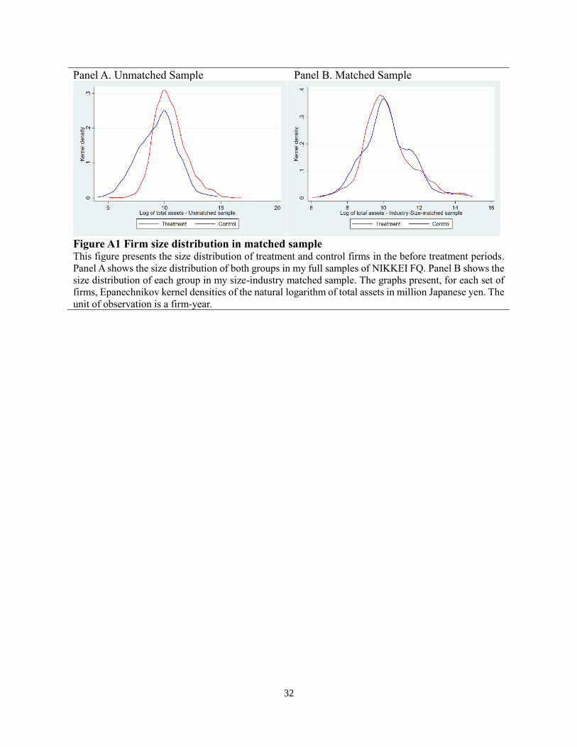
Panel A. Unmatched Sample Panel B. Matched Sample
Figure A1 Firm size distribution in matched sample This figure presents the size distribution of treatment and control firms in the before treatment periods.
Panel A shows the size distribution of both groups in my full samples of NIKKEI FQ. Panel B shows the
size distribution of each group in my size-industry matched sample. The graphs present, for each set of
firms, Epanechnikov kernel densities of the natural logarithm of total assets in million Japanese yen. The
unit of observation is a firm-year.

33
Table A1. Variable definitions This table describes the definitions of the variables in this study.
Variables Definitions
Financing
fin_tot Total financing estimated as the the sum of the cash inflow from loan, issues of bond,
compatible bond, and stock scaled by the sum of lagged tangible and intangible assets.
fin_ext External financing estimated as the sum of the cash inflow from issues of bond, compatible
bond, and stock scaled by the sum of lagged tangible and intangible assets.
fin_loan Bank loan financing estimated as the increase in short- and long-term debt scaled by the sum
of lagged tangible and intangible assets.
Variable in interest
treat Treatment indicator taking one if the firm belongs to treatment group, zero otherwise.
post Post treatment indicator taking one for periods after the treatment year, and 0 for periods prior
to the treatment year.
Control Variables
sg Sales growth estimated the change in sales from the previous fiscal year scaled by the sales
in the previous year.
cfo Operating cash inflow scaled by the sum of lagged tangible and intangible assets.
size The natural logarithm of lagged total assets.
age The natural logarithm of firm age.
cash The sum of cash and short-term security scaled by the sum of lagged tangible and intangible
assets.
lev The sum of short- and long-term debt scaled by the sum of lagged tangible and intangible
assets.
retain Retained earnings scaled by the sum of lagged tangible and intangible assets.
large An indicator taking one if the firm belongs to the first quintile of firm size, zero otherwise.
hp An indicator taking one if the firm belongs to the third quintile of Hadlock-Pierce index, zero
otherwise.
illiq
Amihud Illiquidity index estimated as:
illiq = (1/d) | ret | / (vol × price)]
ret represents daily stock returns, vol represents daily trading volume, price represents the
stock price, and d represents the number of the dates of fiscal year.
ext_depend Rajan and Zingales (1997) external finance dependency estimated as: