financial repression and subsidies: capital...
TRANSCRIPT

FINANCIAL REPRESSION AND SUBSIDIES:
CAPITAL INVESTMENT IN RUSSIA, DECEMBER 1998 TO DECEMBER 2005
By
M. YVONNE REINERTSON
A DISSERTATION PRESENTED TO THE GRADUATE SCHOOL OF THE UNIVERSITY OF FLORIDA IN PARTIAL FULFILLMENT
OF THE REQUIREMENTS FOR THE DEGREE OF DOCTOR OF PHILOSOPHY
UNIVERSITY OF FLORIDA
2007

© 2007 M. Yvonne Reinertson

This dissertation is dedicated to the memory of my mother:
A kinder spirit is not possible.
iv
ACKNOWLEDGMENTS
I am grateful for the guidance of my Chair, Dr. Andy Naranjo, and my Cochair, Dr.
Roy Crum, who made possible my experiences in Russia. I also thank my other
committee members, Dr. Mahendrara Nimalendran, and Dr. Richard Beilock.
Additionally, I would like to thank the following individuals: David Beim, Michael
Bernstam, Charles Calomiris, and Alvin Rabushka. The Russian data used in this
analysis would not have been available without the help of the following Russian friends:
Andrei Betin, Victor Matiashvili, and Roman Vvedensky. I am greatly in their debt.

v
TABLE OF CONTENTS page
ACKNOWLEDGMENTS ................................................................................................. iv
LIST OF TABLES ........................................................................................................... viii
LIST OF FIGURES ........................................................................................................... ix
ABSTRACT .........................................................................................................................x
CHAPTER
1 INTRODUCTION ........................................................................................................1
1.1 Measuring Financial Repression .............................................................................3 1.2 Enterprise Network Socialism ................................................................................4 1.3 Focus of This Work ................................................................................................5
2 DIFFERENCES BETWEEN RUSSIA AND THE UNITED STATES.......................6
2.1 Economic, Banking, and Payment System Structures: Russia versus United States .........................................................................................................................6
2.1.1 Differences: Economic Structure .................................................................7 2.1.2 Differences: Central Bank Monetary Policy Channels ................................9 2.1.3 Differences: Central Bank Balance Sheet ..................................................13 2.1.4 Differences: Payment System .....................................................................14
2.2 Economic, Banking, and Payment System Structures: Role of Gazprom ............16
3 LITERATURE REVIEW ...........................................................................................24
3.1 Financial Repression on Investment: Chronological Changes .............................25 3.1.1 Literature Review: Pre-1998-Default .........................................................26 3.1.2 Literature Review: Post-1998-Default .......................................................28
3.2 Liquidity Constraints on Investment: Government Control of Banking ..............30 3.3 Monetary Policy Transmission on Investment: Primary Channels ......................31
3.3.1 Money Channel ..........................................................................................32 3.3.2 Bank-Lending Channel ...............................................................................32
3.4 Financing Constraints on Investment: Internal versus External Financing ..........33 3.5 Russian Governmental Subsidies .........................................................................38

vi
4 TESTABLE HYPOTHESES ......................................................................................40
4.1 Hypothesis: Financial Repression .........................................................................40 4.2 Hypothesis: Enterprise Network Socialism ..........................................................42 4.3 Systemic Distortions: Gains Possible ...................................................................42 4.4 Analysis: General and Specific Questions ............................................................46
5 DATA .........................................................................................................................49
5.1 Descriptions: Variables .........................................................................................49 5.2 Sources: Data ........................................................................................................50
5.2.1 Russia: Financial Repression Measures and Aggregate Level Capital Investment ........................................................................................................50
5.2.2 Russia: Large Firm Level Capital Investment ............................................51 5.2.3 USA: Financial Repression Measuresand Aggregate Level Capital
Investment ........................................................................................................51 5.2.4 USA: Large Firm Level Capital Investment ..............................................52
6 METHODOLOGY .....................................................................................................54
6.1 Model Notation Conventions ................................................................................56 6.2 Generalized Assumptions: Tested Per Analysis ...................................................58 6.3 Methodology–Time Series for Aggregate Level Investment: ARIMA [AR(1)
Model] .....................................................................................................................59 6.4 Methodology–Panel Data for Firm Level Investment: GLS [Random-Effects
Model] .....................................................................................................................60 6.5 Methodology–Increase Data Interval Frequency: Proportional Denton Method .61
7 RESULTS ...................................................................................................................63
7.1 Aggregate Level Investment–Russia: Descriptive Statistics and Correlations.....63 7.2 Aggregate Level Investment–Russia: Time Series Results ..................................65
7.2.1 Results with Liquidity Variable–Russia: ARIMA [AR(1)] ........................65 7.2.2 Results with Private Borrowing Variable–Russia: ARIMA [AR(1)] .........66
7.3 Large Firm Level Investment–Russia: Descriptive Statistics and Correlations ...67 7.4 Large Firm Level Investment–Russia: Panel Data Results ..................................69
7.4.1 Results with Liquidity Variable–Russia: GLS [Random-Effects] .............69 7.4.2 Results with Private Borrowing Variable–Russia: GLS [Random-
Effects] .............................................................................................................74 7.5 Aggregate Level Investment–USA: Descriptive Statistics and Correlations .......76 7.6 Aggregate Level Investment–USA: Time Series Results .....................................77
7.6.1 Results with Liquidity Variable–USA: ARIMA [AR(1)] ..........................77 7.6.2 Results with Private Borrowing Variable–USA: ARIMA [AR(1)] ...........78
7.7 Large Firm Level Investment–USA: Descriptive Statistics and Correlations ......79 7.8 Large Firm Level Investment–USA: Panel Data Results .....................................80
7.8.1 Results with Liquidity Variable–USA: GLS [Random-Effects] ................80 7.8.2 Results with Private Borrowing Variable–USA: GLS [Random-Effects] .82

vii
7.9 Comparative Statics ..............................................................................................83 7.10 Results: General and Specific Questions ............................................................83
8 CONCLUSION.........................................................................................................101
APPENDIX
A DATA JOURNAL ....................................................................................................105
B DATA: LARGE FIRMS–RUSSIA AND UNITED STATES .................................110
LIST OF REFERENCES .................................................................................................112
BIOGRAPHICAL SKETCH ...........................................................................................118

viii
LIST OF TABLES
Table page 5-1 Variable Definitions .................................................................................................53
7-1 Descriptive statistics and correlation Russia: Aggregate level ................................88
7-2 Estimation Russia: Aggregate level investment–with liquidity variable .................89
7-3 Estimation Russia: Aggregate level investment–with private borrowing variable ..90
7-4 Descriptive statistics and correlation - Russia: Large firm level .............................91
7-5 Estimation - Russia: Large firm level investment–with liquidity variable ..............92
7-6 Estimation – Russia: Large firm level investment–with private borrowing variable .....................................................................................................................93
7-7 Descriptive statistics and correlation USA: Aggregate level ...................................94
7-8 Estimation USA: Aggregate level investment–with liquidity variable ....................95
7-9 Estimation - USA: Aggregate level investment–with private borrowing variable ..96
7-10 Descriptive statistics and correlation USA: Large firm level ..................................97
7-11 Estimation USA: Large firm level investment–with liquidity variable ...................98
7-12 Estimation USA: Large firm level investment–with private borrowing variable ....99
7-13 Comparative statics Expected relationships to investment: Economies of industrialized and transitional countries .................................................................100
B-1 Data: Large firmRussia Russia ...............................................................................110
B-2 Data: Large Firms – USA. ......................................................................................111

ix
LIST OF FIGURES
Figure page 2-1 Monetary Measures from the Monetary Survey (Rubles; billion) ...........................18
2-2 Monetary Measures: M2 (broad) and M0 (narrow) from the CBR; Money and Quasi-money from the Monetary Survey (Rubles; billion)......................................19
2-3 Monetary Survey Components and CBR Total Liability (Rubles; billion) .............20
2-4 Sum of Monetary Survey Components with CBR Total Liability (Rubles; billion) ......................................................................................................................21
2-5 Ratio of Monetary Survey Components to CBR Total Liability .............................22
2-6 Relationship Diagram of the Enterprise Network Socialism ...................................23
4-1 Enterprise Receivables to M2 ..................................................................................47
4-2 Enterprise Receivables to M1 ..................................................................................48
7-1 Monetary Measures: M2 (broad) and M1 (narrow) from the Federal Reserve ........86
7-2 Potential Crowding Out: Private Credit and Total USA Credit ...............................86
7-3 Ratio of Private Credit to Total Credit .....................................................................87
7-4 Industrial Production to GDP ...................................................................................87

x
Abstract of Dissertation Presented to the Graduate School of the University of Florida in Partial Fulfillment of the Requirements for the Degree of Doctor of Philosophy
FINANCIAL REPRESSION AND SUBSIDIES: CAPITAL INVESTMENT IN RUSSIA, DECEMBER 1998 TO DECEMBER 2005
By
M. Yvonne Reinertson
May 2007
Chair: Andy Naranjo Cochair: Roy L. Crum Major: Business Administration
The purpose of this dissertation is to assess potential systemic distortions on
investment from governmental actions of (1) financial repression, and (2) subsidies in
Russia. The extent to which the Russian government engages in policies that, in turn,
stifle investments by firms and other market participants is explored using six individual
proxies (real interest rates, reserve ratio, liquidity, private borrowing, bank lending, and
stock market valuation), which are components of the Beim and Calomiris financial
repression index. Then, subsidy based distortions, theorized in the work of Bernstam and
Rabushka are examined using the results produced by the financial repression study.
Using datasets on both aggregate and firm-level investments in Russia‟s
economy, investment is shown to have a consistently negative association with an
increase in the reserve requirement for both aggregate and large firm investments.
Additionally, and specific to Russian large firms, the data show liquidity and bank

xi
lending are inversely related to capital investment changes. This last result is consistent
with the existence of a subsidy system in Russia producing additional distortions to those
created by the governmental use of financial repression.
The principal objective of banking in any country should be to provide economic
liquidity and investment intermediation. However, in countries where the banks are state
controlled and financial repression is the norm, this objective becomes secondary to
satisfying state budgetary and political goals. This appears to be the case in Russia.
Moreover, the effects of financial repression are magnified by a subsidy system largely
controlled by the country‟s largest firms. Not surprisingly, there is strong evidence of
systemic distortions on investments. The extent to which investments in Russia are
influenced by these effects are highlighted through comparisons with firms in the United
States.
While this research work is specific to Russia, its implications are not. This
examination of financial repression produced distortions addresses an ongoing concern
for many countries, firms, and governmental institutions around the world. Advisors
responsible for designing policy to enhance global economic growth have an interest in
determining the governmental actions that hamper investment. In many nations, primarily
those which are underdeveloped or in transition, governments use repressed domestic
financial systems to fund the state at the expense of private enterprise development.

1
CHAPTER 1 INTRODUCTION
“From the viewpoint of macrostructure, the Russian economy is strongly monopolized through its backbone companies and also Sberbank [nationalized savings bank], which is a monopoly [monopsony as a buyer of household deposits] in its sector. As a result, in every sector, there is little room for competition, and, hence, the economic growth rate is far below its potentially achievable level.”
-Oleg Vyugin, former first deputy chairman of the Central Bank1
Potential economic distortion through government manipulation of monetary
policy, banking intermediation, and financial markets concerns all parties interested in
the growth of transitional and developing countries. Assessing the reality of such
assertions is one of this dissertation‟s two main goals. This will be investigated through
development of financial repression measures for Russia, using both macroeconomic and
microeconomic data (Beim and Calomiris 2001). Building on these results, the second
goal will be addressed by seeking evidence on the possible existence and effects
produced by an enterprise-driven subsidy system called “Enterprise Network Socialism”
(ENS) by Bernstam and Rabushka (1998, 2006).
Financial repression can be loosely defined as governmental actions, either direct
or indirect, taken to restrict or alter the flow-of-funds within an economy. A monopolized
or nationalized banking structure, in Russia‟s case Sberbank, may control both money
stocks and flows. At the start of 2003, state controlled banks in Russia, with Sberbank
being the largest, accounted for “…72 percent of retail deposits, 34 percent of capital, 38
1 Notable Quotes, The Russia Journal, http://www.russiajournal.com (accessed November 2003)

2
percent of assets and 39 percent of credit outstanding to the non-financial private sector”
(Tompson 2004). From the government‟s perspective, a potential benefit of this control is
Sberbank funneling banking deposits into the Russian government treasury. To the
extent that Sberbank‟s assets are directed into government securities, fewer funds are left
from Sberbank to flow into the private sector.
Thus, while the death of the Soviet Union and the following industrial
privatizations removed the extreme form of central control and reduced the monopolistic
structure in many industries, it did not remove tight governmental ties to the banking
industry. Concerning the banking structure and its effect on industrial Russia, Bernstam
and Rabushka (1998, p. 52) have this to say:
The banking system–a winding maze of borrower ownership of banks, insider lending, rollover of bad loans, misallocation of credit, lack of competitive credit markets, and lack of long-term investment and credit-impeded the development of the new private sector… Misallocation of credit and depletion of real deposits
deprived productive users of credit and investment. A vicious circle developed that perpetuated bad credit, reinforced financial repression, and depressed the real sector. Most emerging private firms were forced to self-finance or organize informal arrangements with individuals.2
While this research is specific to Russia, its implications are not. In many nations,
primarily those which are underdeveloped or in transition, governments use repressed
domestic financial systems to fund the state at the expense of private enterprise
development. Ostensibly, the monetary controls that produce financial repression within a
country are intended to facilitate realization of state goals, which may include programs
that are intended to advance legitimate social and economic causes, such as regional
2 In addition to their book, Bernstam and Rabushka maintain an Web site of their research at www.russiaeconomy.org

3
development. However, the controls limit the abilities for both financial institutions and
financial markets to optimally allocate funds to private industry.
1.1 Measuring Financial Repression
The extent to which governments engage in financially repressive policies that in
turn stifle investments by firms and other market participants is an ongoing concern in
many countries. Historically, the existence and extent of financial repression was gauged
by the existence and degree to which real interest rates were negative. The definition of
what constitutes financial repression has expanded to include an array of governmental
actions that preserve tight control of both money stocks and flows and repress the
development of financing sources other than the state controlled banks. These actions
include placing ceilings on deposit interest rates, requiring high reserves from banks,
directing bank credit, government ownership of banks, restricting financial industry
development, and, finally, restraining international capital flows. Beim and Calomiris
(2001) have created an index of financial repression based upon the following six
financial repression proxies: real interest rates, reserve ratio, liquidity, private borrowing,
bank lending, and stock market valuation.3 Using these six proxies individually, it is
possible to evaluate the degree of financial repression in Russia and to explore the effects
of repression on company investment.
In Russia‟s largely cash-based economy, as in many other countries with
developing economies, virtually all credit is only available to a few of the largest firms.
In Russia, these large firms have publicly traded stock listed on the Russian Trading
3 In this research, economic liquidity is measured as M2/GDP. It is an aggregate liquidity measure and defined fully in Appendix A. For a complete explanation of each governmental action and the subsequent proxy, see Beim and Calomiris, 2001, pp. 47-66.

4
System (RTS). The rest of the domestic economy consists of small and medium
enterprises (SME) that are largely limited to internally produce funding sources, or less
formal and usually exorbitant alternatives.
1.2 Enterprise Network Socialism
The second purpose of this dissertation is to assess the potential for systemic
distortions produced through enterprise-driven subsidies. In “Fixing Russia‟s Banks: A
Proposal for Growth” (1998) and their other works, Bernstam and Rabushka have studied
extensively the relationship between the monopolized banking sector and excessive
invoicing in a tax non-remittance subsidy scheme that they call “Enterprise Network
Socialism” (ENS) (2006, chapter 2, p. 4).4 The enterprises involved in the ENS subsidy
constitute a network of the large and dominant firms in Russia. Specific to the enterprise
network effects, Bernstam and Rabushka state:
The enterprise network converts trade credit into a subsidy operation. Enterprises issue overdraft invoices in excess of cash flow available per regular payment period of about one month. Payments fall into arrears. The average length of trade payments expanded to about four months during 1992-1998 and shortened to under three months during 1999-2002. Arrears create the payment jam (2006, chapter 1 addendum, 1).
[Additionally,] Payment arrears between enterprises force subsidies from the government. The more enterprises succeed at wringing the subsidy the more overdraft invoices they issue in order to build up arrears. …overdraft invoices carry
price increases. This reduces real spending during each given period of time, which expresses itself in payment arrears (2006, chapter 1 addendum, 2).
[Specific to this research,] In Russia in 1999, the stock of receivables, which entailed cross-subsidies, was equal to 40 percent of GDP and some 27 percent of total sales, with the average length of payment about 3.5 months and the velocity (turnover) of 3.4 payments per year (2006, p. 23).
4 Enterprise Network Socialism theory by Bernstam and Rabushka (2006) describes a network of enterprises that have used enterprise receivables to redistributing national income.

5
In a market based financial system driven by supply and demand, the subsidy
network, and the gains received, would end. The existence of this system partly explains
Russian entrepreneurial development stalling and the bank restructure process stagnating
15 years after the Soviet Union‟s collapse.
1.3 Focus of This Work
This dissertation examines the effects of financial repression and the ENS subsidy
network on aggregate and firm-level investment in Russia. A dataset will be used which
will permit exploration of the effects of both on aggregate and firm-level investments in
Russia‟s economy. For comparison, the same effects are explored using data from the
United States. Moreover, a Denton proportional interpolation method is used to produce
databases with increased interval frequency (e.g., annual interpolated to quarterly) for
further comparison.
This research fills the following gaps in the literature by investigating (1)
financial repression on two levels of investment within one transitional country, and (2)
Russia‟s subsidy system to large firms. Also, it indirectly adds to the studies of (3)
systemic economic distortion produced through monetary policy manipulations from both
government-instituted financial repression and enterprise-driven subsidies.

6
CHAPTER 2 DIFFERENCES BETWEEN RUSSIA AND THE UNITED STATES
There is a consistently high non-monetary transaction component within Russia‟s
economic structure that makes the Russian payment system unusual. For this reason, a
comparison with a developed Western economy, such as the United States, is appropriate.
2.1 Economic, Banking, and Payment System Structures: Russia versus United States
The single biggest difference between Russia‟s economy and the United States‟
economy is the high degrees to which non-monetary transactions permeate all sectors in
Russia.5 Previous studies have documented barter and trade credits being used in illiquid
economies (Commander and Mumssen 2002). Additionally, in their barter research,
Commander and Mumssen found that banking rollover of enterprise loan arrears made
tracking both the information about the contract stipulations and the true levels of
transactions involved difficult. The difficulty of the banking system being used to
facilitate surrogate money transactions adds to the lack of transparency. That, along with
the repeated exchange of debt contracts to offset taxes or expenses, sanctioned by
Russian civil code, adds to doubts about the accuracy of information on the levels of non-
monetary transactions (Commander and Mumssen 2002). An additional reason for
concern about the quality of information on non-monetary transactions is that collecting
data on this issue can be dangerous (Perotti 2003, p.3). For these reasons, inferences
5 Non-monetary transaction describes economic exchanges being made either through pure barter (exchange a good for another good), or through documents other than the government sanctioned currency. These documents have various IOU properties with specific financial requirements (e.g., maturity date and discount rate).

7
about the actual levels of non-monetary transactions will have to be made from aggregate
data. In Russia, non-monetary transactions take any of the following forms: (1) barter
(goods for goods), (2) money surrogates (veksels, which are commodity or financial
promissory notes issued by enterprises, banks or government), (3) mutual offsets
(zachety, which are used to clear trade, or tax, obligations by exchanging debt for goods),
and (4) debt swaps, sales and roll-overs of previously issued non-monetary documents
(Commander and Mumssen 2002, p.2).
Much of the existing research on illiquidity and chronic non-payment in a non-
transparent structure, seen in Russia, is from the Karpov commission report completed in
1997. As an example, and quoted in Gaddy and Ickes (1998, p. 56), the Karpov
commission stated that “An economy is emerging where prices are charged which no one
pays in cash; where no one pays anything on time; where huge mutual debts are created
that also can‟t be paid off in reasonable periods of time; where wages are declared and
not paid, and so on….” On the CBR balance sheet, non-monetary transaction totals are
identified as „quasi-money.‟6
2.1.1 Differences: Economic Structure
Despite periodic increases in regulatory controls, the United States has
overwhelmingly maintained an open market system based on private ownership. Since
the fall of the Soviet Union, Russia has had a semi-capitalistic system which might be
characterized as market-oriented socialism. Despite a general loosening of controls since
the end of the Soviet Union, there still are high levels of centralized control through
public ownership of property and production inputs.
6 In this dissertation, quasi-money describes the aggregate level listed on the CBR balance sheet, of which a large component measures non-monetary transactions. It is banking system deposits which are not directly used for effecting payments and are less liquid than “money.”

8
The CBR and its precursor, Gosbank, have consistently played a dominant role in
direct management of the centralized economic structures. Academic observers, watching
the stages of Russian economic transformation, called Gosbank an “…important
monitoring device…” used to manage the budgets and finances of most Soviet enterprises
(Gregory and Stuart 1980, p. 209).
This monitoring and management by Gosbank was extensive with the requirement
that enterprise investment funds actually flow through the state bank, which then directly
affected the state budget. Additionally, Soviet firms were required to maintain accounts
with Gosbank. These enterprise accounts allowed records of firm profits to flow through
the state bank accounting and then through to the state budget (Gregory and Stuart 1980).
Furthermore, these records of firm profits provided the taxation base. Thus, lack of
independence has historically been an issue for the CBR, and it continues to be an issue
in the post Soviet Union as the control shifts from parliamentary to presidential hands
(Rose 2000). Setting the independence issue aside, Russia‟s central bank has
microeconomic involvement reaching down to enterprise levels unheard of in
economically developed countries. The depth includes, and goes beyond, the recognized
“investment bank” role that central banks often play in emerging market countries for
their governments by forcing both public and private banks to purchase government debt
(Daniels and VanHoose 2002, p. 229).
Bernstam, in a personal correspondence, wrote “much if not everything in
Russia‟s economic system is topsy-turvy (e.g., net receivables in the flows of funds are
counter-cyclical). Looks like enterprises make more sales and purchases when the
economy contracts and less when the economy recovers, which would have been an

9
obvious, even if ridiculous, interpretation in other economies, but in Russia it simply
means that inflationary expectations and payments arrears went from high to low.”7
Even at the point of deepest regulation in the economic history of United States,
regulations, at most, restricted economic freedoms in isolated industries. In sharp
contrast, the Russian tentacle-like economic structure, however, reaches deep into the
operations of enterprises. For example, Beim and Calomiris (2001) note that the Russian
tax collection process is arbitrary to the extent that some firms receive hidden subsidies
while others, destructive vengeance.
2.1.2 Differences: Central Bank Monetary Policy Channels
Countries with developed economic structures and financial markets often use
indirect methods and channels to conduct monetary policy. In the United States, the usual
channel is through the financial markets using open market operations where U.S.
government securities are bought and sold. Countries with developing economic
structures and emerging financial markets typically use more direct methods because the
financial markets are not sufficiently developed. Argued in this dissertation and
supporting the work of Beim and Calomiris, the insufficient development of financial
market structures is caused, in part, from government use of financial repression to
stymie financial industry growth, and thus subsequently creating systemic distortions.
Furthermore, Roubini and Sala-i-Martin (1995) find support for the possibility of policy-
induced distortions in the flow of savings to investment channel.
When open market operations are not available, the more direct monetary policy
channels are used by central banks. With respect to the money-creation channel and the
7 Email to author dated March 2005.

10
bank-lending channel, the following are typical: (1) Reserve requirement adjustments to
the portions of transactions (checking) and term deposits (time and savings) that banks
must hold either as vault cash or as funds on deposit at the central bank, (2) Interest rate
regulations on depositor funds, and (3) Direct credit controls that constrain the quantity of
credit extended to individuals and firms by the banking system (Daniels and VanHoose
2002). However, atypical ones also apply. Specific to Russia, and applicable to other
illiquid economies, the primary monetary transmission channel and money creation of
currency in circulation is through debt issuance to the nationalized banks (Bernstam and
Rabushka, 2006, chapter 1 addendum 1, p. 6).
Empirically, both the direct and indirect transmission of monetary controls have
been found to affect investment by slowing the economy and controlling both internal
and external funding source availability (Schiantarelli 1996). Additionally, and
supporting claims being made in this research, constrained investment, especially through
the direct transmission in the bank lending channel, falls heavily on small firms. Because
they are without access to other funding sources, small firms are more dependent on the
intermediation provided by a sound commercial banking system (Kashyap and Stein
1994).
To understand the structure of the money supply in Russia, a breakdown of the
Monetary Survey components of money and quasi-money is useful. In Figure 2-1, the
level and growth of quasi-money closely matches the same for the money measure. The
Monetary Survey statistics differ from the usual statistics reported by country central

11
banks, including the CBR, in that it specifically surveys for an approximation of the
quasi-money used in Russia.8
A further comparison between Monetary Survey components and the statistics
typically reported by the CBR is shown in Figure 2-2. Note that while the monetary
survey statistic „money‟ is comparable to the CBR M2, as a measure of money, it is
lower. An extension from this is to consider the actual ruble level within money to be
lower than the M0 reported by the CBR. Thus, the true level of monies available for
economic transactions could possibly be far less than is officially stated.
As explained in Bernstam and Rabushka (2006), the Russian money supply has
grown since 1998 from the increased repatriation requirement of export earnings
mandated by the CBR. This requirement brought back export-generated dollars to be
exchanged for rubles within Russia rather than maintaining the dollars abroad as foreign
currency. With more export earnings returning to Russia‟s economy, along with the
resulting required purchase of rubles, there have been increases in the broad money
supply. However, the increase in the liquid money supply of currency in circulation,
which the small firms depend on for self-financing, is slight.
Additionally and not often thought of as a usual monetary policy channel, there
are central bank sterilization policies.9 Russia, like China, has a managed exchange rate
with an inconvertible currency and large inflows of U.S. dollars. However, unlike
China‟s sterilizing technique of sending incoming U.S. dollars back out of the country to
purchase U.S. treasuries, Russia is keeping the dollars obtained from the forced
8 The monetary survey methodology complies with the IMF Special Data Dissemination Standard (SDDS). 9 Monetary sterilization describes a form of monetary action in which a central bank attempts to insulate itself from the foreign exchange market to counteract the effects of a changing monetary base.

12
repatriation requirement in the country. Following that, the chosen sterilization procedure
by the CBR is to reduce the domestic money supply by selling, when possible, ruble
denominated government bonds. This reduces the supply of rubles available to domestic
firms. On the subject of sterilization, Bernstam wrote, “a comparison of sterilization
methods in China vs. Russia is relevant and useful. But [also] that Russia accumulates
U.S. treasuries in foreign exchange reserves, in addition to monetizing payments and
sterilizing rubles. Both countries have net capital outflow. China‟s is due to an
exceptionally high saving rate which exceeds its exceptionally high investment. Russia‟s
capital outflow depends on the mandated repatriation rate and, as Ron McKinnon
quipped, Russia‟s capital outflow is motivated by pure capital flight.”10 Reflected in
Figure 2-2., compared to the broader measures of aggregate money supply growth, the
liquid ruble growth, M0, is far slower.
This research documents that while the overall broad ruble money supply
increases, the narrow money supply, and thus the source of cash in the Russian economy,
has slower growth and a large non-monetary component. Therefore, cash in the economy,
needed for self-financing investment through internally generated funds, suffers in a
system which tends to keep money inflows as foreign exchange at the CBR. Concern for
the illiquid nature of Russia‟s economy extends to enterprises that will provide future
growth. Specifically, while the small firms are not privy to the subsidy network, the
monetary environment produced affects them. In partially sterilizing the resulting
inflowing funds to keep the U.S. dollars as foreign exchange, the Russian monetary
authorities used ruble denominated bonds and other techniques to reduce the domestic
10 Email to author dated October 2005.

13
money supply. A decrease of the domestic aggregate liquidity increases the use of non-
monetary transactions and reduces the ability to finance capital investment internally.
This supports the findings that available internal funds matter more to firms working in
countries with poorly developed financial systems (Love and Zicchino 2002). The
important point is that the primary negative effects to economic growth will be through
the reduction of small firm growth. As is well-documented, small firms are crucial to
economic growth for industrialized countries. In the United States as an example, small
firms produce fifty percent of the output and account for over fifty percent of the
employment (FED 2002).
2.1.3 Differences: Central Bank Balance Sheet
The core difference between the balance sheet structures of Russia and the United
States is the lack of a line item for quasi-money on the Federal Reserve balance sheet.
Quasi-money is not listed on the CB balance sheet for any of the large developed
countries (e.g., Japan, European System of Central Banks) (Daniels and VanHoose 2002,
p.221). Liquid economies with relatively small black markets do not depend on IOUs
being passed for economic transactions. Studying the quantity, and growth, of quasi-
money on the CBR‟s balance sheet can provide insight into the depth of involvement the
banking system and non-monetary transactions have to enterprise operations and finance.
As is shown in Figure 2.3, even after the increase of forced repatriated export earnings,
the relative size of quasi-money to money has consistently been maintained by the parties
to the Russian payment system.
Focusing on the liability side of the CBR balance sheet, the growth of quasi-
money to CBR total liabilities matches the growth of money to CBR total liability.
Shown in Figure 2.4, and as a ratio in Figure 2.5, the sum of money and quasi-money

14
actually exceeds the total liabilities of the CBR. While this is unique to Russia‟s payment
system, Bernstam and Rabushka (2006) suspect that it is possibly common, albeit to a
lesser degree, in the other former Soviet Union countries.
Typical of central bank balance sheets, while the actual amounts will fluctuate
over time, the proportions of liabilities and equity to assets remain stable (Daniels and
VanHoose 2002). The majority of the assets usually listed on a central bank‟s balance
sheet are governmental securities, and the majority of the liabilities and equity listed are
the liabilities of the government sanctioned currency, with bank reserve deposits often
being the next largest liability. In the case of the CBR, quasi-money is usually on a par
with the Russian currency. The persistence of large volumes of quasi-money, both
absolutely and relative to other liabilities, on the Central Bank balance sheet gives an
indication of the persistence of non-monetary transactions. Additionally, and most
importantly, a possible indicator of the level of non-monetary transactions being
conducted outside the banking system can be seen in the spread between the sum of the
monetary components and the CBR total liabilities shown in Figure 2-4.
2.1.4 Differences: Payment System
Again, the principal difference between the United States and the Russian systems
is the prevalence of non-monetary transactions in the latter. At all levels of economic
activity, from government, banking, enterprises, and households, non-monetary
documents are important to facilitate exchanging goods and services. Reproduced in
Figure 2-6 is a flow diagram by Bernstam and Rabushka that aids in understanding the
non-monetary transfer process. Figure 2-6 represents Russia‟s payment system and the
notational conventions are the following: (1) Relationships between flows are indicated

15
by the plus and minus signs, (2) Red numbers indicate consumption flows, and (3) Blue
numbers represent production flows.
The flows relevant to production (blue numbered in Figure 2-6) taken by the
parties to the Enterprise Network Socialism (ENS) are the following:11
1. First flow: Trade credit separates from sales and production. Invoices outgrow payments when enterprises add a third party surcharge to the price and bill the government.
2. Second flow: The flow of receivables for many enterprises exceeds net income.
They increase payables to prevent their net cash flows from turning negative. Aged receivables increase payment arrears and vice versa. Enterprises whose flow of receivables exceeds that of trade payables must increase tax payables.
3. Third flow: Enterprises do not remit taxes withheld from workers and collected
from consumers. The government cannot enforce full tax remittance.
4. Fourth flow: The government is forced to issue debt (i.e., securitize tax non-remittance).
5. Fifth flow: To delay the default, the government is forced to monetize the budget
deficit, that is, to monetize enterprise tax remittance.
6. Sixth flow: Banks transmit, extend, and roll over credit, which reduces aged receivables.
7. Seventh flow: Variable trade-offs between tax non-remittance and monetization
of tax remittance, followed by credit rollover and extension, wind up in the self-enforceable subsidy. It sums up to the outstanding balances of receivables. A complementary array of cross-industry price subsidies accompanies this subsidy.
8. Eighth flow: [This flow] is identical to step 1. Stimulated by all these
components, enterprises surcharge invoices with a network tax to extract the self-enforceable subsidy. This system becomes circular and self-reinforcing (Bernstam and Rabushka, 2006, chapter 1 addendum 1, p. 6).
9. Ninth flow: [Flows nine through eleven occur after the CBR increased the
mandated repatriation of export earnings in late 1998.] Enterprise money balances in bank accounts expanded.
10. Tenth flow: Enterprise export earnings started to monetize tax remittance.
11 For details on the consumption (red numbered) flows, see Bernstam and Rabushka (2006).

16
11. Eleventh flow: The link between monetization and the tax subsidy was weakened
(Bernstam and Rabushka, 2006, chapter 1 addendum 1, p.33).
Noted in the flow diagram is the importance the banking industry has in
maintaining the ENS; banks, managed by the CBR, are directly involved in half of the
flows. While bank discounting is one element, the other element is non-monetary
documents, especially veksels, which allow barter exchanges in a manner which
facilitates tax avoidance. Thus, while banking is an important part of the maintenance of
ENS, it is equally important to realize that non-monetary exchanges also occur entirely
outside of the banking system. These exchanges occur between all economic parties:
Government, CBR, Banks (both private and public), enterprises, and households. An
indicator of the size of the exchanges occurring outside of the banking system is the
spread between the sum of monetary survey components and the CBR Total Liabilities in
Figure 2-4. Explored in this dissertation is the systemic distortion still evident even after
the increased repatriation requirement in late 1998 by the CBR.
2.2 Economic, Banking, and Payment System Structures: Role of Gazprom
An additional primary player in maintaining the Russian subsidy system is
Gazprom. Natural gas is important both as consumption good and as an industrial input.
In the literature, Gazprom plays an extended role in that, like the Yukos oil, gas payables
and receivables were often used as payment documents. Similar to price adjustments for
veksels above the cash clearance price, gas payables and receivables were exchanged for
elevated values. Through this mechanism, firms would able to increase prices charged
over the price for cash (Commander and Mumssen 2002; Gaddy and Ickes 1998). Noted
in the Karpov commission report, and cited since, is the liquidity issue within barter
goods. The more liquid barter goods are, the more they are used in barter and as quasi-

17
money and as offsets. Not surprisingly, therefore, non-monetary transactions have been
particularly significant in the following: gas, electric power, ferrous metallurgy,
chemistry, and machine-building (Gaddy and Ickes 1998). The Karpov commission
results also show high quasi-monetary transactions in the petroleum, and extractive,
industries. In fact, during the time of the Karpov commission research even Yukos
engineers were being paid with containers of oil.12
The non-monetary documents, such as veksels, allow Gazprom and other firms to
change prices with them because they are not required to be cashed out. They can be used
as negotiating documents with the value being adjusted to satisfy the parties. Often the
stated value is adjusted up to adjust for the discounting banks will calculate when, or if,
the veksel is cashed out (Commander and Mumssen 2002). Systemic distortion, produced
by financial repression and subsidies of monetary or non-monetary values, will affect all
levels of enterprises. Since small firms have more limited access to the commercial bank
lending, they are doubly harmed in illiquid monetary environments. Research has shown
that a liquidity squeeze and the resulting credit crunch can cause businesses and
individuals to shift from monetary to non-monetary transactions (Commander and
Mumssen 2002).
12 Personal communication with Russian individuals revealed to this author the level of barter conducted at the household level. Barter prevalence allowed continued sustenance.

18
0.0
500.0
1000.0
1500.0
2000.0
2500.0
3000.0
3500.0
4000.0
1998m
12
1999m
6
1999m
12
2000m
6
2000m
12
2001m
6
2001m
12
2002m
6
2002m
12
2003m
6
2003m
12
2004m
6
2004m
12
2005m
6
2005m
12
Money(R; bn)
Quasi-money (R; bn)
Figure 2-1. Monetary Measures from the Monetary Survey (Rubles; billion)

19
0.000
1000.000
2000.000
3000.000
4000.000
5000.000
6000.000
1998
m12
1999
m6
1999
m12
2000
m6
2000
m12
2001
m6
2001
m12
2002
m6
2002
m12
2003
m6
2003
m12
2004
m6
2004
m12
2005
m6
2005
m12
M2 (R; bn) Money(R; bn)
Q-money (R; bn) M0 (R; bn)
Figure 2-2. Monetary Measures: M2 (broad) and M0 (narrow) from the CBR; Money and
Quasi-money from the Monetary Survey (Rubles; billion)

20
0.0
1000.0
2000.0
3000.0
4000.0
5000.0
6000.0
1998
m12
1999
m6
1999
m12
2000
m6
2000
m12
2001
m6
2001
m12
2002
m6
2002
m12
2003
m6
2003
m12
2004
m6
2004
m12
2005
m6
2005
m12
Money(R; bn)
Q-money (R; bn) CBR TL(R; bn)
Figure 2-3. Monetary Survey Components and CBR Total Liability (Rubles; billion)

21
0.0
1000.0
2000.0
3000.0
4000.0
5000.0
6000.0
7000.0
8000.0
9000.0
10000.0
1998
m12
1999
m6
1999
m12
2000
m6
2000
m12
2001
m6
2001
m12
2002
m6
2002
m12
2003
m6
2003
m12
2004
m6
2004
m12
2005
m6
2005
m12
Money +Q-money(R; bn)
CBR TL(R; bn)
Figure 2-4. Sum of Monetary Survey Components with CBR Total Liability (Rubles; billion)

22
1.45
1.50
1.55
1.60
1.65
1.70
1998
m12
1999
m6
1999
m12
2000
m6
2000
m12
2001
m6
2001
m12
2002
m6
2002
m12
2003
m6
2003
m12
2004
m6
2004
m12
2005
m6
2005
m12
Figure 2-5. Ratio of Monetary Survey Components to CBR Total Liability

23
Figure 2-6. Relationship Diagram of the Enterprise Network Socialism [Reprinted with
permission from M. Bernstam, and A. Rabushka 2006. From Predation to Prosperity: How to Move from Socialism to Markets. Work in Progress (Page 67, Box 4). The Hoover Institution, Stanford, California.]

24
CHAPTER 3 LITERATURE REVIEW
The literature on capital account and financial market liberalization is extensive
and decades long. The reciprocal literature for financial repression is chronologically
shorter, but it is equally broad. Overwhelmingly, most of the work is on the investment or
economic expansions possible from liberalizing the capital account and/or the financial
markets. In developing countries, existing restrictions are often severe as can be seen in
Beim and Calomiris‟s cross-sectional work. There is less research on the restrictions on
investment produced by new constraints imposed by current or recent governments. It is
critical to develop better knowledge about the mechanics of repressive policies, their
effects, and the incentives structures that initiate and perpetuate them. These are the
subjects of this research, and as such, are an extension to the literature started by Edward
Shaw and Ronald McKinnon in the 1970s, and has since been expanded by the work of
Ross Levine, Robert King, and William Easterly.
The focus of this literature review will be on the following five topics as they
apply to the investment theme:
1. Definitions and opinions of financial liberalization, and its reciprocal, financial repression, before and after the 1997-1998 Asian crisis and Russian default,
2. Primary monetary policy transmission channels on investment: Money (interest
rate) and bank-lending,
3. Liquidity constraints on investment: Government control of banking,
4. Financing constraints on investment: Internal versus external financing, and
5. Government subsidies unique to Russia.

25
Topics one and two describe the status of the current literature relative to
investment in countries with emerging economies. Topics three and four are specific to
the two most severe constraints of illiquidity and financial unavailability common to the
less developed nations. In a sense, the financial repression indicators examined in this
research also take this dichotomy. The first three variables ---- real interest rates, reserve
ratio, and liquidity ---- are proxies for the governmental control over the monetary policy,
which affects the financial system; the last three variables ---- private borrowing, bank
lending, and stock market valuation ---- are proxies for external financing sources.
Finally, the fifth topic describes the magnitude of the government subsidy in Russia.
Liberalization and financial repression research almost exclusively relies on
aggregate investment data in cross-country analyzes. Often absent from these studies are
the transitional countries. This research closes a portion of this gap in the literature by
studying one nation, Russia, and examines financial repression at both the macro and
micro level.
3.1 Financial Repression on Investment: Chronological Changes
Financial repression is the actions taken by a government to alter the flow of a
country‟s money supply to fund government expenses or finance favored investments,
often at the expense of domestic enterprise development. Over the years, the definition of
financial repression has expanded from a monetary policy that produces negative real
interest rates into a broader one that also covers manipulations of the different monetary
policy variables previously stated, which includes interest rates. This broadening of
actions which constitute financial repression is recognition that there are several possible
approaches to pervert the financial sector.

26
This study uses the broader definition of financial repression and focuses on the
post-1998-default period. After that default, monetary policy recommendations took a
dramatic turn. During the 1997-1998 Asian financial crisis and Russian default, the
literature went from support for open flows of both goods and money, to support for
moderation in money flows with the necessary legal and regulatory structure.
3.1.1 Literature Review: Pre-1998-Default
The pre-default literature is supportive of fully liberalizing both the capital
account and financial markets to fund investment and, thus, economic growth. In these
regards, the seminal works are McKinnon‟s 1973 paper for the Brookings Institution and
Shaw‟s book of the same year. Their works are based on the narrow definition of
financial repression. Both authors assert that deposit interest rates held below market
level will produce an inadequate supply of savings to satisfy investment demand. They
also claim that financial liberalization would allow available money to flow to its highest
and best uses.
Subsequent empirical evidence has tended to support the second claim; however,
there is some evidence the first one does not hold once the negative real interest rates on
deposits drop down to single digits. Further, evidence provided by Japan‟s lost decade
suggests a contracting economy can occur even when real interest rates are high and
positive.
In the more recent literature, the question of the “inadequate supply of savings” is
still in doubt. In their study of banking and growth, Beck, Levine, and Loayza (2000) find
savings allocation to have a large impact on real per capita GDP growth. However, like
the earlier research, they find less of an association between the same growth measure
and the quantity of savings deposited into banks. In such investigations, including this

27
research, the view should be from the borrower‟s viewpoint as a cost to borrowing. While
the interest rate ceiling on deposits harms savers and domestic investors, borrowers
benefit from negative real interest rates on ruble deposits. This is particularly true of
large firms in extractive industries as their outputs typically are dollarized. For these large
firms, negative real interest rates mean extremely low costs of borrowing. Further,
inflation from keeping a debased ruble creates conditions in which domestic trade suffers
relative to the extractive export trade. Firms that export prefer a domestically weak
currency. This preference influences the currency policy that a government maintains,
even at the expense of the domestic economy, particularly small firms. The impacts on
less favored borrowers (i.e., smaller firms) can be severe because the same policies which
make borrowing so attractive to larger firms (particularly those focused on exporting)
discourages savers from committing funds in the Russian banking system. In part, this
may explain why so many manufacturing firms in Russia are still using aged and obsolete
machinery.
Two other pieces of pre-default literature are of interest to this research. The first
one is the Roubini and Sala-i-Martin (1995) model of inflation, tax evasion, and financial
repression. They show that governments have incentives to repress a country‟s financial
systems to access an easy source of funds for the public budget through the inflation tax
created through seigniorage taxation.13 And, the second piece is a paper by DeGregorio
and Guidotti (1992) who found a negative association between liberalizing a country‟s
money controls and private sector growth. They claimed that bankers produced the crisis,
13 Seigniorage is the net revenue for a government when the money that is created is worth more than it costs to produce it; seigniorage can be seen as a form of tax levied on the holders of a currency, and as such a redistribution of resources to the issuer.

28
in an unregulated financial system, by choosing projects for loans on the potential return
without considering the connecting project risk.
3.1.2 Literature Review: Post-1998-Default
Since the 1997-98 Asian financial crisis and the Russian default, there has been a
shift in opinions from advising total capital and financial liberalizations to liberalization
only under a structured system of governmental regulatory and legal reforms to ensure a
stable flow of capital. Among the supporters for this new view is Joseph E. Stiglitz (1999,
p. 1509) who states that “the international financial architecture has exhibited enormous
fragility over the past quarter century.” Results from studies of previous financial crises
generally indicate that financial liberalization can be destabilizing. The following six
factors, mentioned in the literature, and cited by Beim and Calomiris (2001, p. 119),
address potential problems with liberalization and list the solutions requiring financial
restrictions in order to maintain financial system stability:
1. Controls on deposit interest rates to provide rents to banks. This makes the banks
more profitable and arguably less vulnerable to failure,
2. Bank reserves to provide the central bank with revenues and a liquidity pool to help banks that get into trouble,
3. Government monitoring the bank lending decisions to prevent fraud and excessive
risk taking,
4. Controls to prevent banks from becoming centers of industrial empires as bank owners use their lending power to buy recently privatized state owned enterprises (SOEs) for themselves,
5. Some controls should be in place to avoid having foreign banks out-compete
domestic banks, leaving them seriously weakened,
6. Capital inflows, particularly short-term loans and portfolio flows, should be monitored with a view to avoiding serious reversals that could create a major liquidity crisis.

29
Implicit in the preceding list of safeguards are the assumptions that governments
are both technically competent and benevolent. Particularly in developing nations, the
first assumption may not hold. Moreover, individuals, either within governments, or
having influence over governments, may have incentives to redirect capital flows to
either preserve or initiate repressive policies to fund government expenditures or provide
favors to private individuals or enterprises.
An important country comparison study, written pre-default but supportive of the
post-default consensus, is by McKinnon. In 1994, McKinnon employed a ratio of a
financial liberalization index to the inflation rate to compare China to some of the former
Soviet Union republics. While financial liberalization in the former was moderate and
controlled, the same process in the latter-was neither. In his results, McKinnon found
China to have low inflation with high economic growth and the reverse in the former
Soviet Union countries.
An important segment of the post-default research has focused on bank fragility
with the overall findings indicating reduced banking vulnerability is possible with
“structured” financial liberalization. These structures include: (1) Strong institutional and
regulatory environment,14 (2) Societal respect for the rule of law, (3) Low-level of
corruption, and (4) Binding contract enforcement (Demirgüç-Kunt and Detragiache
1998). Edison (2004) and his coauthors find in their meta-analysis on previous
liberalization studies, government reputation, as a measure closely linked to quality of
14 In particular, Demirgüç-Kunt and Detragiache (1998) caution financial liberalization, even after macroeconomic stabilization has been obtained, when the following institutions have not been fully developed: laws to ensure contract enforcement, and regulations to produce effective banking sector and financial market supervision.

30
institutions, to be a significant variable. Unfortunately, most of these studies, including
Edison‟s meta-analysis, did not include former Soviet Union countries.
3.2 Liquidity Constraints on Investment: Government Control of Banking
Liquidity does not have a single definition. In reference to financial securities,
liquidity refers to the ability to trade a security without incurring large transaction costs.
In monetary economics, it refers to the most tradable of financial assets-cash (or near-
cash). In this research, the definition used describes the monetary aggregate ratio of
money supply to an economic output measure, usually gross domestic product (GDP).
This gauge for liquidity is often considered a reasonable measure of financial depth
within an economy, typically associated with greater economic and financial system
development (Beim and Calomiris 2001). With the numerator being determined by
monetary policy, transmitted through the money and bank lending channels, bank
ownership becomes critical in determining the funding available for enterprise
investment. In this regard, in Russia the banks that matter tend to have high degrees of
State ownership.
Recent political theories concerning reasons for government ownership of banks
stress controlled investment of the country‟s enterprises and the subsequent political
kickbacks as the primary incentives. Furthermore, research on global banking finds
government ownership to be positively associated with poorly operating financial
systems and negatively correlated with efficient capital allocation to investments. In their
research on the prevalence of government ownership in developing countries, La Porta,
Lopez-De-Silanes, and Shleifer (2002) support these views. Additionally and specific to
Russia, Laeven (2001) finds heavy insider lending and bribery compensation between
banker and borrower. The findings contradict the previously theorized development view

31
of governments principally directing scarce resources to productive enterprise projects in
desired industries, and to then further ascribe positive social goals as the primary
motivations for government bank ownership (Barth, Caprio, and Levine 1999; Wurgler
2000).
This line of research supports the bank competition literature, which claims that
competition, in either foreign or domestically owned banks, is necessary in generating
investment and economic growth (Beck, Demirgüç-Kunt, and Maksimovic 2004c;
Berger, Hasan, and Klapper 2004). Indicative of the extent of this effect is the finding by
Smith (1998) that a country with a monopolistic banking system of any ownership type
produces macroeconomic performance worse than an economy void of banks.
In many developing nations, government ownership of banks is typically high,
and the domestic money supply that reaches down to the household and enterprise level is
often tight (Beim and Calomiris 2001). While the money supply growth is sufficient to
produce significant inflation, the direction of the monetary growth is back to the
government coffers. This can result from required purchase of government securities by
the state owned banks. These characteristics are true for Russia. Additionally, it will be
argued here that it is government control of the financial system, and banking in
particular, that allows the Enterprise Network Socialism (ENS) subsidy network to work.
3.3 Monetary Policy Transmission on Investment: Primary Channels
Developing economies are excellent testing grounds for monetary policy
transmission research. In these countries, monetary controls generally are the tightest.
Additionally, it is in these economies that the traditional interest rate effects in the money
channel continue to be a mode of transmission in affecting the real interest rate, as well as

32
from within the bank-lending channel.15 This is possible because banking is typically the
sole formal external financing form in these countries. The financial repression manifests
itself through interest rates different from free market levels. Controls on interest rates are
applied by and through the banking segment of the financial system.
3.3.1 Money Channel
Two studies are chosen for review here for both the money and bank channels. In
a study on Germany, Chirinko, and von Kalckreuth (2003) test the traditional interest rate
effects in the money channel on business fixed investment. They find a statistically
significant interest rate channel on a database of over 6,000 German businesses, and a
credit channel for a subset of the companies. Honohan (1998), in a study of countries
whose governments are liberalizing both the capital accounts and the financial markets,
finds support for the money channel form of monetary policy transmission. Within this
channel, he finds dramatic short-term volatility increases in the money market. Treasury
bill interest rates, with bank spreads, tended to increase the most, implying that they were
the securities most repressed.
3.3.2 Bank-Lending Channel
Support is also found for the bank-lending channel as a monetary transmission
mechanism. Kashyap and Stein (2000) find the impact of monetary policy through the
bank-lending channel is greatest on small banks. In countries with developing economies
where small banks dominate and the few large banks are State controlled, the bank-
lending channel becomes a powerful conduit for monetary policy transmission.
15 For a detailed explanation of the various monetary policy channels, see chapter 25 of Mishkin (2003).

33
Driscoll (2004) tests the relationship between individual U.S. state output and the
supply of bank loans. He finds that the relationship is often statistically insignificant
after controlling for shocks to the money demand. It is important to realize, however, that
in developing economies, where government controls over the money supply is both tight
and through banking, transaction money demand may take the form of plain barter. To
continue, from these findings, Driscoll (2004, p. 469) suggests that when alternative
sources of funding are available, and enterprises are no longer bank loan dependent,
monetary policy transmission goes through a broader credit channel. The findings of
Kashyap and Stein (2000), as well as, Driscoll, suggest that the bank-lending channel
effect at the enterprise level is weaker for large firms that have alternatives to bank
lending for project and investment funding. Additionally, the effect becomes
progressively weaker as the firm is able to move up through bank sizes into using the
international money and capital markets.
3.4 Financing Constraints on Investment: Internal versus External Financing16
Early research in the internal versus external financing debate includes
Dobrovolsky (1958), Cohen (1968), and Waite (1973). All found an increase in the
external finance comparable in importance with internally derived funds. These early
papers also noted differences in the funding sources available to large firms versus small
firms.
A chronological divide between internal and external financing is obvious in the
literature. Research in the early part of the last decade is more specific to internal
16 For a comprehensive survey on business constraints (finance, taxation, and corruption) on global firms, see Batra, G., D. Kaufmann, A. Stone, 2003, “The Firms Speak: What the World Business Environment Survey Tells Us about Constraints on Private Sector Development,” World Bank Working Paper Series

34
financing constraints. Some of the works have included the difficulties of asymmetric
information, capital market imperfections, and agency problems. Whited (1992) takes the
early research on liquidity constraints and connects asymmetric information to it. From
the findings, he states that adverse selection constraints that affect the bond market also
affect an enterprise‟s ability to get needed funds. Studies of internal finance and R&D
expenditure generally find that internal financing takes a leading role because of capital
market imperfections. This is especially true for small high-tech enterprises
(Himmelberg, and Petersen 1994). Hubbard, Kashyap, and Whited (1995) find agency
costs unimportant for business fixed investment of enterprises that have significant
dividend payouts. However, agency costs do seem to be a factor for enterprises in a low-
dividend-payout subsample. Some studies support the theoretical agency cost link
between investment and internal finance. Considering asymmetrical information effects
in their study, Calomiris and Hubbard (1990) find a high likelihood the interest rate does
not reflect the “shadow price of credit.” They also find that credit rationing is probable.
Bernanke and Gertler (1990) find that high agency costs produce low and inefficient
investments for enterprises that have a heavy reliance on external finance. Finally, using
hospital investment in support of the results found in the manufacturing sector, Calem,
and Rizzo (1995) show a link between significant agency costs in capital markets and
tight internal investment funds.
Kaplan and Zingales (1997) find that less financially constrained enterprises are
more sensitive to investment-cash flow changes than enterprises that are more financially
constrained. In support of this research, Cleary (1999) finds enterprise investment to be

35
directly related to financial factors with high credit rated enterprises being more sensitive
to shifting internal funds than that of lower credit rated enterprises.
Moving on to the external finance thread of the literature, Fazzari, Hubbard, and
Petersen (1988) and Fazzari and Petersen (1993) examine the relationship between
financial constraints and investment. These studies find strong impacts from finance
constraints on growth and investment, and that internal finance and external finance are
not perfect substitutes, especially in the short run. Additionally, Bond and Meghir (1994)
developed a hierarchical finance model which predicts that in any period a subset of
enterprises will have constrained investment from a lack of internally derived funds.
Besides the agency theory aspect of this topic, legal structure, profitability, and
enterprise size are also used as determining criteria of financing source availability. All
three are found to be significant factors, with, not surprisingly, lower profitability
indicating a need for external funding. In particular, Fauver, Houston and Naranjo (2003)
find the value of firm diversification is related to the legal systems, as well as, to the
depth and level of capital market development and international integration. Furthermore,
they find optimal firm organizational structure may differ for firms operating in emerging
market countries more than for firms operating in established market countries with
international integration.
Stock markets and banks differ in their external finance provisions and effects,
and both are important (Demirgüç-Kunt, and Maksimovic 1998, and 2002; Beck, and
Levine 2002; Claessen, Djankov, and Lang 2000). Love and other World Bank
researchers find that capital account controls increase enterprise financing constraints, but
that multinational firms are not constrained (Harrison, Love, and McMillan 2004).

36
Further, Love (2003) finds that financial development (liberalization) influences growth
by reducing financial constraints that would negatively affect investment. Additionally,
using a vector autoregression technique, Love and Zicchino (2002) find financial
constraints on enterprise level investment to be larger in countries with less developed
financial systems.
In addition to supporting the need for developed financial systems, financial
intermediaries in particular, Levine, Loayza, and Beck (2000) find both strong legal and
accounting systems to be positively associated with economic growth. Lastly, in
studying the effects of monetary policy transmission on inventory investment, Kashyap,
Lamont, and Stein (1994) find tight money supply to be positively associated to liquidity-
constrained inventory investment. Again, as noted in the previous literature cited,
transitional countries are absent from the databases used in these studies.
In sector specific research, recent studies find support for higher growth of
enterprises dependent on external finance when producing within countries with
developed financial markets (Beck, Levine, and Loayza 2000; Galindo, Micco, and
Ordoñez 2002). Rajan and Zingales (1998) find the primary benefit of financial
development regarding external finance to enterprises to be that of cost reduction. And,
Galindo, Schiantarelli, and Weiss (2003) find most of financial reforms increased
investment allocation efficiency within enterprises.
Papers that study, and compare, small firm versus large firm reaction to monetary
changes often confirm the suspicion that financial liberalization affects small and large
firms differently. Since small firms do not have access to the financing choices available
the larger firms, they are relatively more constrained because of a country‟s monetary

37
controls. Laeven (2003) found that larger firms may suffer relatively after liberalization.
With the removal of controls, their comparative advantage over smaller firms in securing
financing is reduced. Similarly, Beck, Demirgüç-Kunt, and Maksimovic (2004b) find
small firms are most affected by financial constraints, as well as, legal and corruption
issues.
In their study of finance and growth, King and Levine (1993) affirm Joseph
Schumpeter in his claim that financial intermediaries oiled the economic wheel.
Schumpeter‟s claim is also supported in Levine‟s (1997, p. 688) later work with his
statement that there is a “positive, first-order relationship between financial development
and economic growth.” He further states there is a “… growing body of work would push
even skeptics toward the belief that the development of financial markets and institutions
is a critical and inextricable part of the growth process….”
Recent research continues to search for the optimal allocation of financing in
investment and economic growth. The optimal allocation work is in an attempt to
determine when short-term funding is better than the longer-term for investment (Fisman
and Love 2004). Most enterprises operating in countries with emerging markets typically
have only the short-term funding variety available from local banks and so are vulnerable
to constraints. Found to be resistant to funding constraints and currency crises are older,
larger, and foreign owned enterprises (Beck, Demirgüç-Kunt, Laeven, and Maksimovic
2004a; Desai, Foley, and Forbes 2004). In developing countries with repressed financial
markets, it is the entire investment environment that is constrained, not just industry
segments. In these countries with cash based economies, often with cash shortages, the

38
funding issue is not internal versus external financing of business as being optimal;
instead, it is financing through barter.
3.5 Russian Governmental Subsidies
In addition to Bernstam and Rabushka‟s work discussed throughout this research,
others have studied the extensiveness of non-monetary economies and the use of
subsidies within broader transitional country studies.17 The notion of a Russian “virtual”
economy began with the work by Gaddy and Ickes (1998). They observed that while the
Russian economy seemed to be recovering from the initial fall in real GDP during the
early 1990s, a non-monetary payment and subsidy system was also expanding.
In the Russian studies, including the initial work by Gaddy and Ickes, authors
repeatedly note the expanding tax arrears by the energy monopolies. The large extractive
sector enterprises collect taxes from customers but fail to remit those taxes collected to
the government. The arrears form an implicit subsidy and expand the tax delinquent level
of the participant enterprises by passing the related costs on to the Russian government‟s
fiscal accounts. Additionally, a repeated relationship feedback loop from setting
economic goal to recovery from policy failure and then back again is noted (Pinto,
Drebentsov, and Morozov 2001; Schaffer 1995). While macroeconomic stabilization and
microeconomic minimization of social costs were the goals, policy failures involving
chronic shortfalls in cash tax collections fed a feedback into a rise in public debt. The
macroeconomic tools of fixed exchange rate and tight credit conflicted with the
microeconomic minimization tools of avoiding mass enterprise bankruptcy through 17 The broad studies include publications by both IMF and The World Bank. In his work at the IMF, Stanley Fischer and coauthors produced a stream of research on economic growth within the transitional countries. They begin by painting a bleak picture of falling real GDP to rising inflation in their 1996 publication to reporting in a 2002 working paper that higher growth is dependent of structural reforms in general and privatization in particular. This same picture is echoed by the World Bank (1996).

39
implicit subsidies. Thus, the feedback loop that Pinto, Drebentsov, and Morozov (2001)
reported fed through enterprises as they faced liquidity and credit squeezes from the
monetary policies, and then fed through to higher subsidies needed, which then fed the
increasing public debt and tax revenue shortfalls, to then repeat the loop–but at a higher
monetary layer.
Finally, the subsidy literature supports the claim made in this research that it is the
individuals with vested interests who are privy to the benefits that hold the subsidy
structure in place. While the distortions have been well documented, the recommended
economic and monetary restructuring have repeatedly, and deliberately, been stalled.

40
CHAPTER 4 TESTABLE HYPOTHESES
This research has two purposes. The first purpose is to examine the distortionary
effects on Russian investment of financial repression, which is measured by the six
financial repression components (real interest rates, reserve ratio, economic liquidity,
private borrowing, bank lending, and stock market value). The second purpose is to
explore the distortion arising from the Enterprise Network Socialism using inferences
from the examination of the financial repression measures and effects. Thus, in this
dissertation, potential systemic distortions on investment produced from governmental
actions of both (1) financial repression, and (2) subsidies are examined. This examination
is further subdivided into the following: (1) Within financial repression, how
government‟s direct control over the first three components affect the indirect control
over the development of the last three, and (2) Within subsidies, how the system is
bidirectional between government entities and enterprises.
4.1 Hypothesis: Financial Repression
The first set of hypotheses address the influence of financial repression on
Russian investment at the aggregate and firm levels after the 1998 Russian default. With
45 as the severity breakpoint, previous research finds that Russia‟s financial repression
index dropped from a near severe 48.1 measure in 1997 into a severe 36.8 by 1998 (Beim
and Calomiris 2001).18 This suggests that during the financial default, the Russian
18 For index details, see chapter 2 appendix in Beim and Calomiris (2001).

41
government may have chosen to choke off funding from the entire country. Whether
deliberate or otherwise, with the currency debased, liquidity plummeted and barter
soared. Building on this line of reasoning, the following hypothesis is explored with
regard to financial repression: In the literature, Beim and Calomiris (2001) found an
increasingly repressive index for Russia. Extending their work, it is theorized in this
research that repression impacts the levels and structure of investment. In other words, it
is theorized that financial repression has a significant distortionary effect on the
allocation of capital.
An interesting subdivision in the financial repression hypothesis is a grouping that
indicates possible effects to the last three financial repression indicators (private
borrowing, bank lending and stock market valuation) from the actions taken by the CBR
on the first three (real interest rates, reserve ratio, economic liquidity). The Central Bank
has direct control on the levels of the first three financial repression indicators through
direct changes to the interest rates and required reserve ratios. Those changes affect the
money supply and thus, liquidity. The last three financial repression indicators are
measures of the level of financial market development, which is affected by the direct
control of the first three by the CBR. The first three components could be considered as
indicators of a government‟s control over monetary policy, and the last three as external
financing development indicators. Bank and financial market development are affected
by the control of real interest rates, reserve ratio, economic liquidity. Within this division,
the alternative to the typical null hypothesis of zero effects is that monetary policies that
repress both the financial development of a country and the available external financing
sources impact on aggregate economic and enterprise level investment.

42
4.2 Hypothesis: Enterprise Network Socialism
The Enterprise Network Socialism (ENS) hypothesis is based on the theory that
an economic structure that allows a “…misallocation of credit and depletion of real
deposits deprived productive users of credit and investment,” and “most emerging private
firms were forced to self-finance or organize informal arrangements with individuals,”
with “payment arrears between enterprises that force subsidies from the government” will
produce potential systemic distortions (e.g., unusual investment relationships to external
funding measures) (Bernstam and Rabushka 1998, p. 52; and 2006, chapter 1 addendum,
p. 2). The hypothesis explored in this dissertation is: In the literature, Bernstam and
Rabushka‟s (1998, 2006) ENS subsidy system is theorized to distort economic growth in
Russia. Extending their work to investment by using inferences drawn from the financial
repression results, the hypothesis is that the ENS subsidy compounds the financial
repression distortions.
An interesting subdivision in the governmental subsidy distortion hypothesis is
that the subsidy system unique to Russia is bidirectional between government entities and
enterprises. Alluded to in the above quotes from Bernstam and Rabushka, Russian
enterprises are able to force subsidies from government. Partly a holdover from
procedures typical to the Soviet Union, and partly a recent creation produced during the
privatization years when prices were released from central control, the system is self-
enforcing and, as theorized by Bernstam and Rabushka (1998, 2006), can generate
extreme outcomes.
4.3 Systemic Distortions: Gains Possible
The gains from financial repression can pass to the Russian government. The
potential advantage Russia‟s government has in preserving financial repression is the

43
ability to fund government expenses through control of the country‟s financial system.
Repression, with capital controls and regulations, allows the Russian government to
restrict financial intermediation and prevent potential competition to the State-controlled
banks from developing.19 An added benefit to the government is that these actions are
often inflationary, which allows the government to pay claims with cheaper rubles. Aptly
stated and relevant to Russia, Roubini and Sala-i-Martin (1995, p. 277) claim that
financial repression is associated with high inflation, high tax evasion, and low growth.
They also claim that the “potential source of easy resources” further encourages
governments to continue financial repression methods. Additionally, concerning financial
repression, Roubini and Sala-i-Martin (1995, p. 277) state:
It is our view that the main reason why governments stay in the way of private financial evolution is that the financial sector is the potential source of “easy”
resources for the public budget. Governments have the power to follow policies of financial repression. By financial repression we mean that they have the option
and capability of not allowing the financial sector to operate at its full potential
by introducing all kinds of regulations, laws, and other nonmarket restrictions to
the behavior of banks and other general financial intermediaries. Thus, the inflationary effect allows the government to pay the remaining fiscal expenses
with a debased currency.
The gains from the ENS subsidy system pass to the subsidized Russian large
firms. As the Figures 4-1 and 4-2 show, the invoicing between Russian large firms and
the Central Bank of Russia (CBR) is significant. The quantity of trade receivables
submitted by the enterprise network equals, and often even exceeds, the sum of tax non-
remittance and the money supply measures, M2 and M1. Since 2003, increases in
19 In basic banking, intermediation describes household savings efficiently allocated to economically productive private enterprise. However, in Russia, “…banks are akin to business enterprises but shuffle
financial instruments for their own profit instead of producing real goods and services” (Bernstam, and Rabushka 1998, p. 17).

44
petroleum dollars continue to fill foreign reserves reflected in the broader measure M2;
however, much slower growth in M1, see Figure 4-2, indicates an illiquid Russian
economy. The subsidy process affects economic liquidity by being multiplied through the
banking system as loans to the enterprises. The loans involved are both new and old, with
the old ones rolled-over at maturity. An added distortion is attributed to many of the
rolled-over loans being permanently non-performing. In Russia, the CBR and the large
firms use the commercial banking system to re-intermediate the large firm subsidy.20
Little retail banking, needed by small firms, occurs. Furthermore, at times the quantity of
over-invoiced receivables submitted by the enterprises for the subsidy exceed the “total
bank credit and the entire ruble money stock” (Bernstam, and Rabushka 1998, p. 11).
Additionally, the invoice pricing represents, to some extent, a recovery from the price
caps that are still required by the Russian government for subsidized consumption to both
businesses and households. The ENS subsidy firms submit the invoicing to receive the
difference between the perceived market price and the price cap. This perceived market
price is based on the amounts the firms consider the Russian government‟s price payment
tolerance.
Bernstam and Rabushka (2006) note that the massive size of the receivables has
repeatedly caused financial havoc to the point of halting the economy by creating a
payment jam in the credit system. This occurs when the mass of receivables expands in
size and lengthens the payment arrears from buyer to seller. In effect the large firms in
the receivables network have a degree of control over the tax base.
20 In Russian banking, re-intermediate describes “…channeling household funds to the government and government subsidies to enterprises…” (Bernstam, and Rabushka 1998, p. 20).

45
In this research, it is argued that financial repression and the ENS subsidy are
supportive of one another. The ENS network could not function in a country with a fully
market-based intermediating banking system. Therefore, the argument explored in this
research is that the financially repressive measures taken through the Russian
monopolized banking and financial system sustain the ENS and its self-enforcing subsidy
system. Furthermore, without the first distortion produced by financial repression, which
benefits the Russia government, the second distortion produced by the subsidy system,
which benefits the extracting sector enterprises, would end. Additionally, the
combination of these two produce a third distortion with global implications: restricting
money availability in a cash-based economy hampers small firm growth.
Since financial repression produced by government actions coexist with the
control over the tax base produced by the actions of the ENS subsidy network firms, both
will be reviewed in the appropriate results section in this dissertation. Breaking apart the
two effects is difficult. In this research, the assumption will be made that the statistical
significance of a variable coefficient supports the possible effects of both financial
repression and the ENS subsidy on investment. Coefficients counter intuitive to finance
and economic development theory will be assumed to support the existence of distortions
created by the forced subsidies.
The dangers of systemic distortions to economic growth can be severe.
Schumpeter‟s view that developed financial systems of banking, bonds, and stocks, are
important to economic growth has been supported in academic research (King and Levine
1993). When a country‟s banking system, as the first financial system to typically

46
develop, is used to re-intermediate a subsidy rather than intermediate efficient allocation
of capital, economic growth suffers.
4.4 Analysis: General and Specific Questions
In exploring the stated hypotheses of potential systemic distortion from financial
repression and governmental subsidies, the general questions of interest are the
following: (1) Are there differences between Russia, with its emerging financial markets
and systems, and the United States, with established financial markets and systems? (2)
Within Russia, are there differences between the aggregate level and the large firm level?
Further, are there differences when compared to the USA results?
In further exploring the stated hypotheses, the specific research questions of
interest in are the following: (1) Within Russia, which of the financial repression
components (real interest rates, reserve ratio, economic liquidity, private borrowing, bank
lending, and stock market value) matter to each level of investment? Further, are there
differences when compared to the USA results? (2) Within Russia, is there evidence of
systemic distortions consistent with the existence of the Russian ENS subsidy?

47
Figure 4-1. Enterprise Receivables to M2 [Reprinted with permission from M. Bernstam,
and A. Rabushka 2006. From Predation to Prosperity: How to Move from Socialism to Markets. Work in Progress (Page 62, Figure 13-1). The Hoover Institution, Stanford, California.]
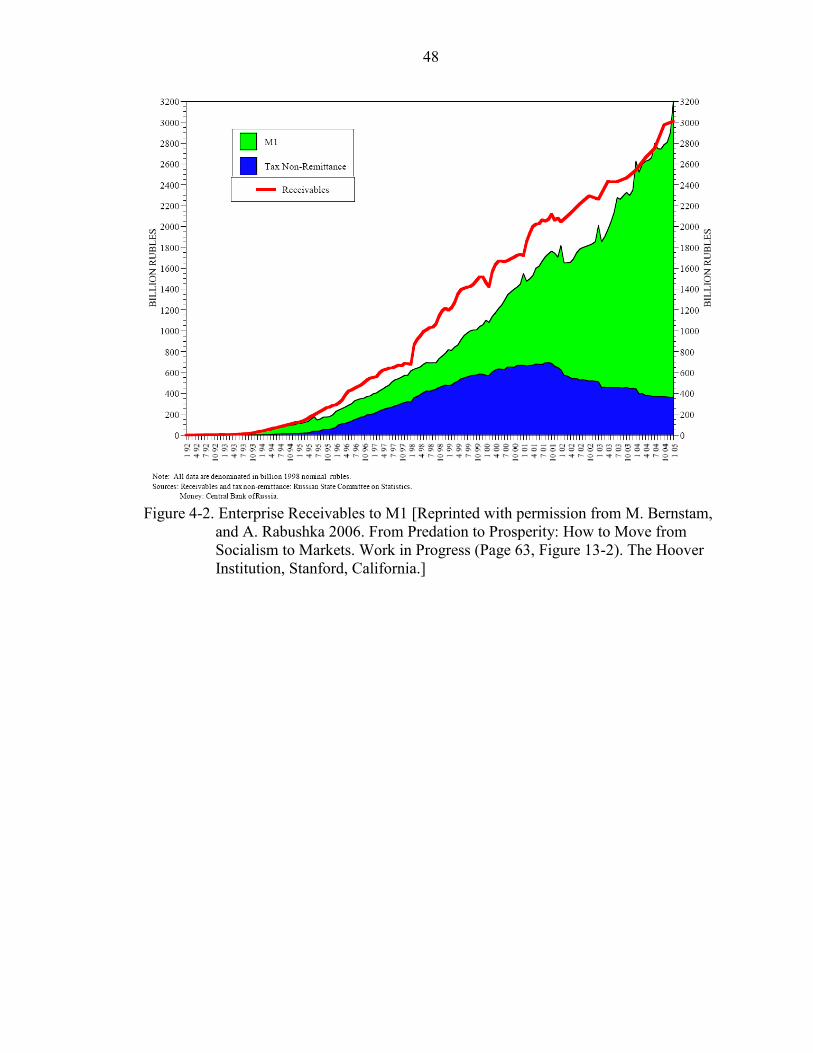
48
Figure 4-2. Enterprise Receivables to M1 [Reprinted with permission from M. Bernstam,
and A. Rabushka 2006. From Predation to Prosperity: How to Move from Socialism to Markets. Work in Progress (Page 63, Figure 13-2). The Hoover Institution, Stanford, California.]

49
CHAPTER 5 DATA
Data for this research are used to estimate the degrees and dimensions of financial
repression in Russia, as well as their determinants and investment effects at the aggregate
and firm level in Russia. Inferences are drawn from the results to confirm or reject the
hypotheses for financial repression and the Enterprise Network Socialism (ENS) subsidy
system.
For comparative purposes, a similar database for the U.S. is created. For both the
Russia and USA analyses, a Denton proportional interpolation method is used to produce
databases with increased frequencies (e.g., yearly data interpolated to quarterly). For
consistency, in all databases, the applicable country‟s industrial production is used as the
interpolating variable with the source in all analyses being the respective central banks.
5.1 Descriptions: Variables21
The variable consistently used across all analyses is the capital investment of
fixed assets made at the aggregate and large firm economic levels of both the Russian and
the United States economy. At the aggregate level, it is aggregate investment data as a
component in the gross domestic product (GDP) equation. GDP measures production
within the national boundaries, which includes foreign firms operating within the national
borders. If purely foreign firms account for significant shares of domestic production,
GDP could overstate progress by indigenous firms. However, this is less of a concern
21 See the Data Journal in Appendix A for details and glossary.

50
than usual because the foreign direct investment in Russia has been consistently low, with
most foreign investment restricted to joint ventures with Russian partners.
At the firm level, a form of gross fixed expenditure is used. The investment data
used is the change in plant, property, and equipment (PP&E) expenditure made by the
large publicly traded firms in Russia, and by the Dow Jones 28 non-financial firms in the
United States.
The independent variables are the components that stem from the Beim and
Calomiris (2001) financial repression index. These measures provide indications of the
extent and types of repressive actions in which a government may engage. Assessment of
these measures provides insights into the actions typically taken, or policies issued, by a
country‟s government to repress the financial system. Additionally, the following
variables are included to control for shocks to investment in Russia unrelated to
repressive actions: Real price of oil, and winter temperature extremes. The petroleum
sector is a dominant component of Russia‟s extractive sector economy, and weather
extremes are a potential hindrance to industrial investment and production particularly in
Russia.
5.2 Sources: Data
5.2.1 Russia: Financial Repression Measures and Aggregate Level Capital Investment
The sample period of investigation for the Russian aggregate level analysis is
from December 1998 through December 2005 (29 actual quarters, 85 Denton interpolated
months). The data for all the financial repression measures, along with the aggregate
capital investment measure, come from the Russian Economic Trends database (RET)
database until June 2002. The Russian-European Center for Economic Policy (RECEP)
produced the database for a project that began as the result of an original partnership

51
between the European Community and the Stockholm School of Economics. The original
mandate was to find and disseminate data that was difficult to get from the Russian
government. The publishing outlet was the Russia Economic Trends (RET) quarterly
journal, which originally began as a publication produced by the London School of
Economics in 1992. However, the RET ceased to maintain their database in 2002. For
this reason, data for this research after June 2002 was gathered from the original RET
Russian sources: Central Bank of Russia, and Goskomstat (State Statistical Agency of
Russia).
5.2.2 Russia: Large Firm Level Capital Investment
The sample period of investigation for the Russian large firm level analysis is
from December 1998 through December 2005 (Unbalanced panel data: 8 to 5 actual
years, 29 to 17 Denton interpolated quarters). The data for firm level capital investment
come from the following sources: Worldscope, Global Reports, and Company financials.
Firm investment data come from the Primark (now Thomson) Worldscope
standardized company financials database. Most of the firm data are provided for by
listings in Worldscope, supplemented with data gained directly from the original
company documents.
5.2.3 USA: Financial Repression Measures and Aggregate Level Capital Investment
The sample period of investigation for the USA aggregate level analysis is from
December 1996 through December 2005 (37 actual quarters, 109 Denton interpolated
months). The data for all the financial repression measures, with the aggregate capital
investment measure, come from the following sources: (1) Federal Reserve, and (2) U.S.
Department of Commerce: Bureau of Economic Analysis, and Bureau of Labor Statistics
(BLS).

52
5.2.4 USA: Large Firm Level Capital Investment
The sample period of investigation for the USA large firm level analysis is from
December 1996 through December 2005 (37 actual quarters, 37 Denton interpolated
quarters). The data for firm level capital investment come from Worldscope, SEC, and
company financials.

53
Table 5-1. Variable Definitions Variable Name: Description: Dependent Variable y1 INVESTMENT (y1) Aggregate: Gross fixed investment (logarithm); (y1) Large firms:
Gross fixed investment (scaled by one-period lagged “PP&E” assets)
Independent Variables Ly1 LAGGED Y1 (Ly1) One lag of y1
x1 REAL RATES (x1) Real interest rates: Nominal annual on bank deposits adjusted for
realized annual inflation (one-period lag)
x2 RESERVE RATIO (x2) Reserve ratio: Bank reserves / M2 (Russia: money plus (some) quasi-money; USA: standard M2) less M0 (one-period lag)
x3 LIQUIDITY (x3) Liquidity: Short-term liquid liabilities M2 / GDP (one-period lag)
x4 P. BORROWING (x4) Private borrowing: Claims on private sector / Total domestic credit (one-period lag)
x5B. LENDING (x5) Bank lending: Deposit bank assets / Deposit bank assets plus central bank assets (one-period lag)
x6 MARKET VALUE (x6) Market Value: Aggregate stock market capitalization / GDP (one-period lag)
x7 F. CHARACTERISTIC (x7) Firm characteristic: Total revenue / Total assets (one-period lag)
x8 OIL (x8) Real price for oil (one-period lag) x9 ACCELERATION PRINCIPLE (x9) Acceleration principle: One lag of revenue
x10 SEASONAL (x10) Temperature for seasonal effects

54
CHAPTER 6 METHODOLOGY
As the first focus of this research is in the potential relationships of investment to
financial repression components, the models take on some of the characteristics typical of
models used in investment and financial repression studies. The main difference between
investment and financial repression studies is in the scope. Where financial repression
research focuses on a broader theme of aggregate growth using cross-sectional cross-
country, the usual models in the investment literature are more narrow and specific.
The most common types of investment models are Tobin‟s Q, Euler equations,
and internal liquidity constraints.22 Schiantarelli (1996) notes inconsistencies for both
Tobin‟s Q and Euler equations in his investment constraint survey. Hsiao and
Tahmiscioglu (1997) study the internal liquidity constraint models, in addition to testing
the effects of Tobin‟s Q on capital investment. They then ranked the models typical of the
investment literature by the resulting statistical precision. In this ranking, Hsiao and
Tahmiscioglu (1997) find the liquidity model to have the highest ranking and the Tobin‟s
Q model the lowest. In addition to the inconsistencies, both Tobin‟s Q and the Euler
equation have recognized difficulties. Tobin‟s Q needs a functioning and liquid domestic
22 Tobin‟s Q describes the market value of assets divided by replacement value of assets. A Tobin‟s Q ratio greater than 1 indicates the firm has done well with its investment decisions. Euler equation, as it applies to investment, describes a firm‟s potential financing constraints by assuming that the firm‟s stochastic
discount factor is a function of the firm‟s financial position. Further, its relationship to Tobin‟s Q is a
“…rearrangement of the first-order conditions form the same maximization problem used to derive Q equations” (Schiantarelli 1996, p. 75). Internal liquidity constraints affect investment through low profits, or high dividend payouts, and external liquidity constraints describe the arbitrary limit on the amount a firm can borrow, or an arbitrary alteration in the interest rate they pay (Hsiao and Tahmiscioglu 1997).
55
stock market, which is often not found in transitional countries, and the Euler equation
may not be able to detect the unvarying financial constraints within a study of investment
unless there is “… data over a period of time [that is] long enough to record changes in
individual firms‟ financial strength and overall macroeconomic conditions” (Schiantarelli
1996, p. 77). Because of the difficulties found in these structured models, a more recent
study tends to use a vector autoregression technique on unstructured and reduced form
investment models (Love, and Zicchino 2002).
The investment models examining liquidity constraints have a closer application
to this research. The difference from many of the studies in the literature and this study is
that the liquidity measure, as one of the financial repression constraints, is aggregate
economic rather than internal to the enterprise as in Schiantarelli (1996), Chirinko, and
Schaller (1995), and Hsiao and Tahmiscioglu (1997). Thus, unlike the investment
models, but similar to the financial repression models, this research studies the
macroeconomic constraints to aggregate and firm level investment produced by
government control over the money supply, financial depth, and bank credit. These
liquidity constraints are typical of countries with developing economies working under
financial repression and tight monetary policy, Chirinko and Schaller (1995, p. 528)
observed that “…liquidity is highly correlated with current, hence future, output, it could
be a significant determinant of investment even if firms do not face constraints.” Finally,
typical to investment models in general, the models in this research are all lagged models,
with a t-1 to denote the lag on each independent variable, which provides “time-to-plan”
for investment decisions.
56
In both static and dynamic models, the base investment model performs as a
function of the financial repression measures.
real interest rates, reserve ratio, liquidity,
private borrowing, bank lending, stock market value
1, 2, 3, 4, 5, 6
I f f
f x x x x x x
x (6-1)
Further interpretation of the base investment function in this analysis is the following:
first 3 variables measure government control over monetary policy,
last 3 variables measure possibly effects to external financing
f
(6-2)
This division allows consideration of the possible distortionary effects on external
financing of banking and financial market systems development which can be produced
from the monetary policy controls over real interest rates, reserve ratio requirements, and
economic liquidity. Additional models have exogenous variables added to the base model
to control for possible fundamental effects important to investment in Russia: Real oil
price, and temperature. Furthermore, in an attempt to model the acceleration principle,
investment equations have included lagged revenue (Fazzari, Hubbard, and Petersen
1988). This principle tries to connect investment needs for capital goods to a firm‟s level
of product demand.
6.1 Model Notation Conventions
Throughout this research, matrix notation to multiple regressions is used. And,
with the exception of the vector xt being a row vector, all notations follow the
recommendations made to the Royal Economic Society and stated in Abadir and

57
Magnus‟s (2002) “Econometric Standardization.”23 In notational development from
scalar to full matrix, the following conventions hold:
Scalar Notation: For each model, the t subscript will be used to represent time,
1, 2,..., t T ; the i subscript will be added in the panel data analyses to index
observations, with the n subscript denoting the sample size of those observations,
1, 2,..., i n ; and finally, with k to indicate parameters, 1, 2,...,k K . The scalar model
0 0 1 1 2 2 ... t t t t k tk ty x x x x has a dependent variable for time t of ty , and
each , tkx as an independent variable with xt0 as unity; and finally, t representing the
population disturbance at time t.
Vector Notation: With bolded lowercase, the scalar time-series model, applicable
to the aggregate investment analysis in this research, becomes , 1,2,...,t ty t T tx β .
Each component, further defined, is the following: the xt is a 1 x K row vector of
independent variables 11, ,...,t t tkx xx with xt0 reserved for the leading 1; the K x 1
parameters vector β is 0 1, ,..., K β .
Matrix Notation: When fully generalized, and with bolded uppercase, the same
model becomes: y = Xβ+ε . The defined components then are the following: the T x 1
vector y is observations on y, where an element of y is yt,; a full T x K matrix, X, is
observations on the independent variables, where the tth row of X consists of the vector xt,
and where the element (t, k)th of X is xtk; with the K x 1 parameters vector β, Xβ
becomes T x 1; and finally, εt becomes ε, a T x 1 vector of unobservable disturbances.
23 The econometric standards are attempting to structure standards that mimic those set by The International Organization for Standardization used by scientists in chemistry and physics (Abadir and Magnus 2002, p.76).

58
General notation: E(∙) refers to the expectation of a random variable, while V(∙)
does the same for the variance. Finally, the basic variable names will be used in the body
of this paper with the appropriate time and firm level observation notation added when
appropriate.
6.2 Generalized Assumptions: Tested Per Analysis
Along with the assumption of linearity in the parameters, various diagnostics are
used to test the following set of basic assumptions for the models, E | ,y X Xβ
estimated in this research:
2 2
is the x matrix with rank , and thus no perfect collinearity,
having an error structure of | ~ ( , ), where E | , E |
T K K
N
X
ε X 0 I ε X 0 εε X I
Therefore, the error structure assumptions are the following: normality of errors, where
the expectation of the error structure has a zero conditional mean and homoskedasticity,
without serial correlation.
In addition to the methods listed below, univariate, bivariate and multivariate
diagnostics are completed for both specification and misspecification. To address the
problems that are typical to the data and models used, the standard errors are adjusted for
autocorrelation in the time-series models, and both autocorrelation and heteroskedasticity
in the panel data models by using autocorrelation and heteroskedasticity-consistent
analysis techniques. The diagnostics are correspondingly reported with the appropriate
analysis results.
Methodologies used are the following: (1) autoregressive integrated moving-
average (ARIMA) technique for a first-order autoregressive process [AR (1)] is used for
the aggregate investment time-series analyses. (2) Generalized least squares (GLS)
random-effect is used for the firm level investment panel data analyses. (3) Proportional
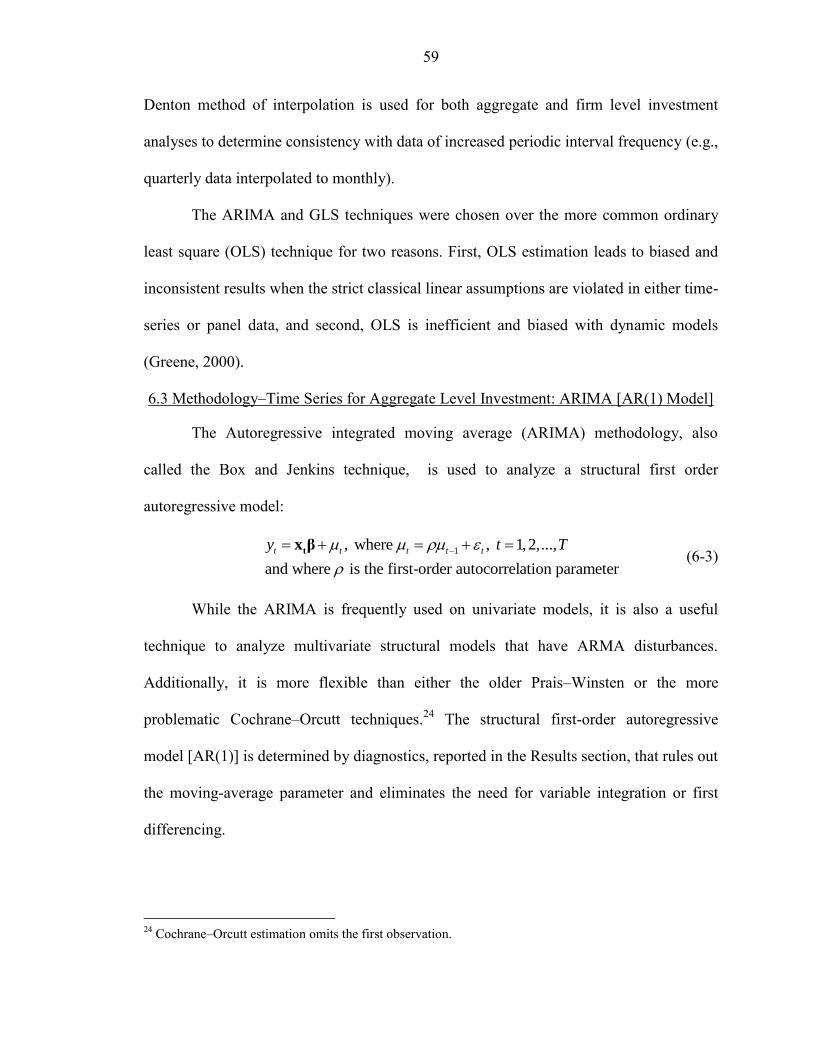
59
Denton method of interpolation is used for both aggregate and firm level investment
analyses to determine consistency with data of increased periodic interval frequency (e.g.,
quarterly data interpolated to monthly).
The ARIMA and GLS techniques were chosen over the more common ordinary
least square (OLS) technique for two reasons. First, OLS estimation leads to biased and
inconsistent results when the strict classical linear assumptions are violated in either time-
series or panel data, and second, OLS is inefficient and biased with dynamic models
(Greene, 2000).
6.3 Methodology–Time Series for Aggregate Level Investment: ARIMA [AR(1) Model]
The Autoregressive integrated moving average (ARIMA) methodology, also
called the Box and Jenkins technique, is used to analyze a structural first order
autoregressive model:
1, where , 1,2,...,
and where is the first-order autocorrelation parameter
t t t t ty t T
t
x β (6-3)
While the ARIMA is frequently used on univariate models, it is also a useful
technique to analyze multivariate structural models that have ARMA disturbances.
Additionally, it is more flexible than either the older Prais–Winsten or the more
problematic Cochrane–Orcutt techniques.24 The structural first-order autoregressive
model [AR(1)] is determined by diagnostics, reported in the Results section, that rules out
the moving-average parameter and eliminates the need for variable integration or first
differencing.
24 Cochrane–Orcutt estimation omits the first observation.

60
6.4 Methodology–Panel Data for Firm Level Investment: GLS [Random-Effects Model]
, for 1,2,..., and 1,2,...,
Where, is the random unit-specific residual and E 0
it i it
i i
y i n t T
itx β
(6-4)
The advantage of using panel data is that it allows investigation of the effects, or
change, of both within and between-firm units. The chosen random-effects model for the
firm level analysis is based on the following: (1) The small number of time waves per
panel precludes the number of indicator variables necessary for a fixed effect model, and
(2) while the monetary policies are time-varying independent variables, because they are
monetary policy variables, they do not vary by much. Still, and reported in the analysis
results section, the Hausman test is used to determine the appropriateness of the random
effects model to the fixed effects. Additionally, specific to this research, Hsiao and
Tahmiscioglu (1997), in their firm level investment study, ran separate regressions on
manufacturing firms in the United States to find out if heterogeneity among firms can be
captured by firm specific intercepts in a fixed effect model. Their findings suggest that it
cannot. However, Hsiao and Tahmiscioglu (1997) do add a lagged capital investment
variable to capture the dynamics of firm investment.
The random-effects model using either the GLS or the maximum likelihood (ML)
method is considered to be a subject-specific model with a random constant term. Of the
two techniques, GLS has the clear advantage over ML in this study in that it does not
need the panels to be long to get consistent estimates of the betas. It also allows the
regressors to be invariant, or in this research, to vary little. Additionally, the GLS version
of the random-effects model is distribution free. Speculation of a distribution for the
individual effect is not necessary (Hsiao 1986). In the correlation structure of the panel

61
data analyses, both autocorrelation and heteroskedasticity typical to panel data analyses
are addressed in the GLS random-effects models.
6.5 Methodology–Increase Data Interval Frequency: Proportional Denton Method
The reasons behind including the proportion Denton method in this research are:
(1) Test for consistency across results, (2) Test for increased statistical precision with the
increase in interval frequency, and thus, an increase in degrees of freedom, and (3) Test
the method as a tool to be used in countries with developing economies where enterprise
financial and operational data are typically only available in annual interval frequencies.
Completed on all datasets, both time-series and panel data: The proportional
Denton method produces an interpolation of an annual time series to quarterly by use of
an associated “indicator series,” imposing the constraints that the interpolated series
obeys the annual total. The same procedure can be used for higher frequencies such as a
quarterly series interpolated to monthly.25 This method is the preferred one of the Denton
family of least-squares-based benchmarking methods because it takes into account the
“existence of any systematic bias [seasonal fluctuations, etc.] or lack thereof” in the
series (Bloem, Dippelsman, and Maehle 2001, p. 84).26 The appropriate industrial
production measure is the indicator series used in this research for both the Russia and
USA models.
The proportional Denton method is a least squares approach: (1) the increased
frequency estimates to be derived are the parameters, and (2) the sum of squares involved
25 Bloem, A., R. Dippelsman, and N. Maehle, 2001, “Quarterly National Accounts Manual: Concepts, Data Sources, and Compilation” International Monetary Fund. See chapter VI on Benchmarking.
26 Benchmarking deals with the problems of combining a series of high-frequency data with a series of less frequent data (Bloem, Dippelsman, and Maehle 2001).

62
are the first differences of the X/I ratio of the interpolated series (X) to the indicator
series (I).
Per Bloem, Dippelsman, and Maehle (2001), and in their notation, mathematically
the proportional Denton formulation for an annual to quarterly interpolation is the
following:
2
1..., 4 ,...
2
1
1
min T
T
t
t tx x x
t tI I
X X
(6-5)
Each formulation is minimized under the restrictions that the sum of the quarters
should be equal to the annual data for each year, and in doing so, the series proportions
are maintained.

63
CHAPTER 7 RESULTS
This research examines the influence of the six financial repression measures on
investment at both the aggregate and large firm level. Inferences drawn from the financial
repression results are then used to examine, Bernstam and Rabushka‟s Enterprise
Network Socialism (ENS) subsidy hypothesis.
On each model previously listed in the Methodology section, and in addition to
the sensitivity analyses performed, the following diagnostic checks are completed for
robustness:
1. The USA database matches the database for Russia aggregate investment and the large firms (Dow Jones 28 non-financial companies) for the United States. The same analyses are then explored on the U.S. data as a comparison test to the Russia research for robustness.
2. The proportional Denton procedure is completed on every database. While
economists, working in developing countries, where data are scarce, use the proportional Denton method, it is not often used with financial data, largely because of the abundance of quality data provided by the financial markets in economically developed countries. The purposes for including the proportional Denton method here are: (1) Examine consistency in results for robustness checks, (2) Examine for increased statistical precision with the increase in both interval frequency and degrees of freedom, and (3) Examine the method as a tool to be used for financial economic research in developing market economies where data is scarce.
7.1 Aggregate Level Investment–Russia: Descriptive Statistics and Correlations
The aggregate level investment descriptive statistics and correlation analysis are
summarized on Table 7-1. Worthy of note is the high positive correlation of 0.79 found
between x3LIQUIDITY, and x4PRIVATE BORROWING. The tremendous size of the ENS subsidy

64
along with the role banking has transmitting the non-monetary surrogate monies may
explain the high correlation found. The Russian government monetizes the subsidy by
issuing bank credit to the large firms. In this case, private borrowing does not have the
usual definition. “Credit to enterprises, subsidized by the government and the CBR,
consumed 99 percent of total credit” (Bernstam and Rabushka 1998, p. 41). Thus, the
liquidity to private borrowing connection is possibly due to the use of the banking system
to pay the subsidies in the form of loans and rolled-over loans. This tangled occurrence
alone has the ability to distort. With that said, and for whatever the reason, the high
correlation is examined here by having a dual set of models in each section. One set
contains the x3LIQUIDITY measure, and the second set contains the x4PRIVATE BORROWING
measure.27
The time series analysis results, listed below, are produced by autocorrelation-
consistent techniques to adjust standard errors. The sensitivity diagnostics completed on
the data used in the models in this section are the following:
Univariate diagnostics were used to test for skewness, data outliers, and
stationarity of both the mean and the variance. The tests were not able to reject the null
hypothesis of symmetrical distribution. The question of stationarity is of primary
importance in using time-series data; therefore, the augmented Dickey-Fuller test is used.
The assumption is that the variables indicate a stationary process because both the
dependent and the independent variables exhibit slow change. This is especially true with
the independent variables being calculated as ratios with monetary components that
27 In addition to the reported liquidity variable, M2/GDP, all analyses were reconfigured using the narrow money measures of M0, and M1, as well as the broadest of money measures, M3. All results are comparable to those reported using M2.

65
typically have slow adjustments to economic changes. The Dickey-Fuller unit root tests
show that the variables, including the real interest rate, are stationary.28
Bivariate diagnostics were used to test sensitivity for correlation. Because of the
unusually high correlation found between x3LIQUIDITY and x4PRIVATE BORROWING, a dual
model structure was used throughout the research. Additionally, correlograms that were
used to evaluate the first-order autocorrelation between current and lagged investment
indicated white noise with no significant autocorrelation.
Multivariate diagnostics were used to test sensitivity for specification,
misspecification and precision. The Portmanteau statistic was calculated for correlation
with the findings indicating white noise errors. The results of this final diagnostic are
presented on the appropriate tables.
7.2 Aggregate Level Investment–Russia: Time Series Results
In most of the models in both the aggregate and large firm level investment the
reserve requirement ratio is the statistically significant independent variable of
prominence. It is the variable that seems to be of great importance across all of Russia.
Other exogenous controls, however, did not indicate a statistical significance. Neither
severe weather, x10SEASONAL, nor previous period petroleum price, x8OIL, mattered in the
investment models for either the aggregate or the firm levels.
7.2.1 Results with Liquidity Variable–Russia: ARIMA [AR(1)]
1
INVESTMENT RESERVE RATIO2 1
, where is the first-order autocorrelation parameter
1 2 ,
t t t
t tty x
xβ (7-1)
28 The autocorrelation function and the partial autocorrelation function verify the Dickey-Fuller results.

66
Per equation 7-1, within the aggregate level investment time series analysis, for
the models that contain x3(t-1)LIQUIDITY as an independent variable, the variable of interest
is the statistically significant x2(t-1)RESERVE RATIO. All insignificant variables are contained
within xβ , which in this equation includes the x3(t-1)LIQUIDITY variable.
Using Model 1 from Table 7-2, the independent variable x2(t-1)RESERVE RATIO has as
coefficient of -2.75 for the Denton interpolated data (-3.34 for the actual data). This
suggests that a 1-unit absolute increase in the required reserve ratio is associated with
over a 2.75 relative decrease in y1(t)INVESTMENT (logarithm) in the following period.
The significance of x2(t-1)RESERVE RATIO, suggests the primary importance this
direct monetary control variable has in countries with underdeveloped financial markets.
The potential for systemic distortion that the typically high reserve requirement has to
investment and economic growth is indicated by having the reserve ratio statistically
significant for all four Russian analyses. These results support the claim by Beim and
Calomiris (2001, p. 51) that reserves paying zero-interest are an “implicit tax on
banking,” and thus the banking system as a whole provides an important source of
“government revenues.”
7.2.2 Results with Private Borrowing Variable–Russia: ARIMA [AR(1)]
1
INVESTMENT RESERVE RATIO2 1
, where is the first-order autocorrelation parameter
1 2 ,
t t t
t tty x
xβ (7-2)
Per equation 7-2, within the time series analysis, for the models that contain x4(t-
1)PRIVATE BORROWING as an independent variable, the measure that matters to the aggregate
level of investment in Russia is the statistically significant x2(t-1)RESERVE RATIO. The same
relationship holds in this model as in the model with liquidity as an independent variable.
Additionally, xβ contains all insignificant variables including the x4(t-1)PRIVATE BORROWING

67
variable in equation 7-2. In Russia‟s aggregate level, only the reserve ratio holds as
having potential effects on investment.
Using Model 1 from Table 7-3, the independent variable x2(t-1)RESERVE RATIO has a
coefficient of -1.45 for the Denton interpolated data (-1.59 for actual data). This suggests
that a 1-unit absolute increase in the required reserve ratio is associated with over a 1.45
relative decrease in y1(t)INVESTMENT (logarithm) in the following period. The results from
equation 7-2 with x4(t-1)PRIVATE BORROWING as an independent variable is comparable to the
results from equation 7-1 containing the x3LIQUIDITY as an independent variable. Of all
the financial repression variables, the reserve ratio as a measure of required reserves
provides the most direct source of monies to a government purse. Beim and Calomiris
(2001, p. 49) notes that having a high reserve requirement on commercial banks reduces
the amount of sovereign debt needed to be issued, and thus, “…reduces government debt
service costs.”
7.3 Large Firm Level Investment–Russia: Descriptive Statistics and Correlations
It is of interest to note on Table 7-4, the consistently negative real interest rates.
Historically, this has been the narrow definition of financial repression. Both McKinnon
and Shaw, beginning in their 1973 publications, focus on the interest rate variable from
the investor‟s viewpoint where the return is to the investor and a positive coefficient is
expected. They viewed the effects produced by deposit interest rate ceilings held below
the level of inflation, as having a negative impact on economic growth, and they then
theorized that negative real rates would have an impact on an investor‟s willingness to
forgo consumption for a negative real return on investment. However, while negative real
interest rates are considered to be the original definition of financial repression, it is also
an indication of the true cost of borrowing for firms. To any size firm, an increasing

68
negative interest rate produces a decreasing true borrowing cost. Additionally, and
relevant to Russia, the dominant extractive sector exporting firms gain by keeping
production, and the resulting costs, in countries with inflationary economies. Throughout
the research period of December 1998 to December 2005, Russian policy results in
inflation and negative real interest rates by preserving a devalued currency and deposit
interest rate ceilings below inflation. The government and the large firms in the ENS,
Russia‟s two largest borrowers, are in the best position to benefit from inflation and
negative real interest rates. In a personal communication, Bernstam stated, “Enterprises
receive a huge subsidy via, inter alia, the negative real lending rates. This is a feature of
subsidized credit. …when inflation is high and nominal interest rates are low, and hence
real interest rates are highly negative, credit rollover and extension represent a pure
subsidy.”29
The panel data analysis results, listed below, are produced by autocorrelation and
heteroskedasticity-consistent techniques to adjust standard errors. The sensitivity
diagnostics completed on the data used in the models in this section are the following:
Univariate diagnostics were used to test sensitivity for skewness, data outliers,
and stationarity of both the mean and the variance. The diagnostics used in this section
address the same concerns with the time-series analysis but with the additional concern of
heteroskedasticity. Because short panels tend to be stationary and with the variables the
same as those used in the aggregate level analyses, the diagnostics produced similar
results. The difference in this analysis is that it is firm-level investment being
29 Email to author dated October 2005.

69
investigated; however, like the aggregate level investment, it also exhibits slow
adjustment to economic changes.
Bivariate diagnostics were used to test sensitivity for correlation. Again, the dual
model structure is used in this research resulted from the finding of high correlation
between x3LIQUIDITY and x4PRIVATE BORROWING.
Multivariate diagnostics were used to test sensitivity for specification,
misspecification and precision. The Hausman specification diagnostic indicated little
difference in the fixed effect model and the random effect model. The final diagnostic,
Collinearity Condition Number (CCN), measuring the eigenvalue and the determinant of
the correlation matrix for each model is reported on the appropriate tables.30
7.4 Large Firm Level Investment–Russia: Panel Data Results
Generally, like the aggregate level of investment, the reserve ratio is also
indicating importance as a financial repression variable to the large firm level investment.
However, in the large firm level results, other variables indicate possible ENS subsidy
system effects.
7.4.1 Results with Liquidity Variable–Russia: GLS [Random-Effects]
INVESTMENT RESERVE RATIO LIQUIDITY BANK LENDING
MARKET VALUE
50 2 1 3 1 1
6 1 where is the random unit-specific residual and E 0
1 2 3 5
6 , i i
it it it it
i itit
y x x x
x
xβ (7-3)
Per equation 7-3, within the large firm level investment analysis, for the models
that contain x3(it-1)LIQUIDITY as an independent variable, the statistically significant
financial repression measures are x2(it-1)RESERVE RATIO, x3(it-1)LIQUIDITY, x5(it-1)BANK LENDING,
and x6(it-1)MARKET VALUE.
30 This analysis is an extension to a previous research of the same models using a database that ended June 2002. The negative coefficients exhibited are a consistent result across both studies.

70
Using Model 3 from Table 7-5, the independent variable x2(it-1)RESERVE RATIO has
as coefficient of -0.5 for Denton interpolated data. This suggests that a 1-unit increase in
bank reserves relative to M2 is associated with over a 0.5 decrease in y1(it)INVESTMENT in
the following period. In the large firm models, the importance of bank reserve
requirements by the CBR to firm level investment indicates an understandably negative
relationship, similar to the findings from aggregate level, but less pronounced. It would
be expected that the increase in the reserve ratio would, by reducing the money supply
available to satisfy consumption demand, negatively affect investment through a
reduction in production.
In addition to the previous period aggregate reserve ratio requirement from the
banking system, the regression results also suggest an economically significant impact on
investment from a change in previous period liquidity. Using Model 3 from Table 7-5,
the independent variable x3(it-1)LIQUIDITY has as coefficient of -0.29 for Denton
interpolated data. This suggests that a 1-unit increase in M2 relative to GDP is associated
with over a 0.29 decrease in y1(it)INVESTMENT in the following period.
The regression results also suggest an economically significant impact on capital
investment to a change in bank lending. Using Model 3 from Table 7-5, the independent
variable x5(it-1)BANK LENDING has as coefficient of -1.98 for the Denton interpolated data.
This suggests that a 1-unit absolute increase in deposit bank assets to the sum of deposit
bank assets and central bank assets is associated with a 1.98 decrease in y1(t)INVESTMENT
in the following period. According to Bernstam and Rabushka (1998), in Russia the
banking system does not intermediate between lender and borrower. Instead, the banks

71
are used to re-intermediate the flow of invoicing from large firms to the CBR, and the
return flow of the subsidy, in the form of loans, from the CBR back to the large firms.
From the above results, the expected relationships on two of the six financial
repression measures, liquidity and bank lending, are counter intuitive to the results
typically observed in economically developed countries. Thus, besides testing the
components in Beim and Calomiris‟s financial repression index, the results of this
research are producing potential support for the Bernstam and Rabushka‟s ENS
hypothesis. These subsidies are a throwback to the Soviet Union era, and are a substantial
part of the Russian accounting standards.
The massive subsidies that pass from the Russian Central Bank to firms are at
least a partial explanation for, and possibly compound, the monetary distortions created
by the financial repressive actions taken by the Russian government. The negative
coefficient on liquidity and on bank lending indicates the possible systemic distortion
financial repression and the ENS subsidy are capable of producing. Considering that the
size of the receivables matches, and occasionally exceeds, the sum of the tax non-
remittance and the most liquid money supply, M1, it is not surprising that variations in
receivables affect the entire Russian economy. This continues to be true even after the
increased petroleum dollars began to fill the foreign reserve vault. Per Bernstam, in a
personal correspondence, on liquidity as capital formation, “… enterprise investment is
largely self-financing (also using a capital consumption allowance and government
capital transfers) while the banking system chiefly recycles enterprise and household
payments and deposits held for payments, re-intermediates rather than intermediates.
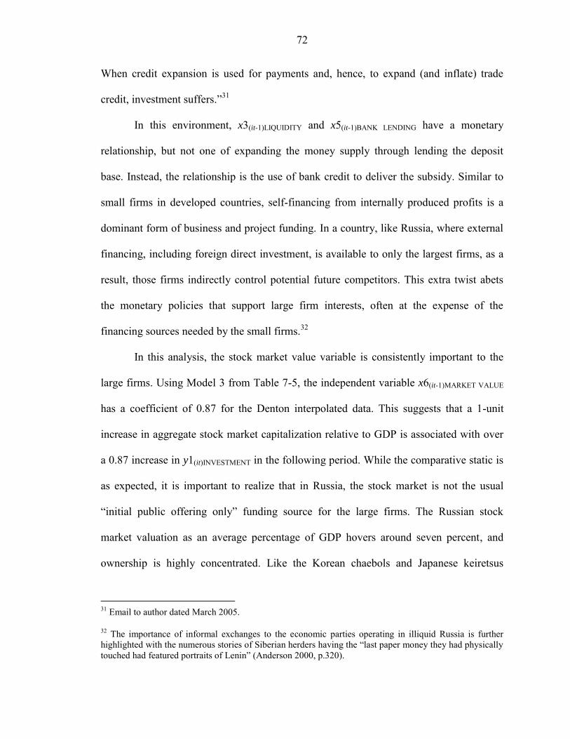
72
When credit expansion is used for payments and, hence, to expand (and inflate) trade
credit, investment suffers.”31
In this environment, x3(it-1)LIQUIDITY and x5(it-1)BANK LENDING have a monetary
relationship, but not one of expanding the money supply through lending the deposit
base. Instead, the relationship is the use of bank credit to deliver the subsidy. Similar to
small firms in developed countries, self-financing from internally produced profits is a
dominant form of business and project funding. In a country, like Russia, where external
financing, including foreign direct investment, is available to only the largest firms, as a
result, those firms indirectly control potential future competitors. This extra twist abets
the monetary policies that support large firm interests, often at the expense of the
financing sources needed by the small firms.32
In this analysis, the stock market value variable is consistently important to the
large firms. Using Model 3 from Table 7-5, the independent variable x6(it-1)MARKET VALUE
has a coefficient of 0.87 for the Denton interpolated data. This suggests that a 1-unit
increase in aggregate stock market capitalization relative to GDP is associated with over
a 0.87 increase in y1(it)INVESTMENT in the following period. While the comparative static is
as expected, it is important to realize that in Russia, the stock market is not the usual
“initial public offering only” funding source for the large firms. The Russian stock
market valuation as an average percentage of GDP hovers around seven percent, and
ownership is highly concentrated. Like the Korean chaebols and Japanese keiretsus
31 Email to author dated March 2005.
32 The importance of informal exchanges to the economic parties operating in illiquid Russia is further highlighted with the numerous stories of Siberian herders having the “last paper money they had physically
touched had featured portraits of Lenin” (Anderson 2000, p.320).

73
before them, a small group of business conglomerates in Russia own and control large
sections of the firms that make up the Russian economy. Additionally, like German
banks, Russian banks own shares. Outside the state controlled banks, the conglomerates
own many of the larger Russian commercial banks. Referred to in the popular press as
“pocket banks,” these banks often own shares of the companies that own them. Thus, the
monetary usefulness of the Russian stock market as a funding source for Russian publicly
traded firms extends beyond the initial public offering. It is also the trading gains
obtained in a manipulated market.33 “In late 1997, when the government desperately
needed to collect tax arrears from the largest enterprise debtors, it did not approach
enterprises but rather squeezed major banks (e.g., Uneximbank, Russian Credit, etc.) and
got paid” (Bernstam and Rabushka 1998, p. 49).
The positive coefficient on the stock market valuation supports the ENS subsidy
hypothesis. Assuming that the Russian government‟s only concern with the stock market
is to restrict its growth and the resulting competition to the government controlled
banking system as a financially repressed component, the stock market component of the
Russian financial system is outside the re-intermediating payment cycle of the self-
enforcing ENS subsidy. Thus, the coefficient is as expected, as probably would be the
signs on x3(it-1)LIQUIDITY and x5(it-1)BANK LENDING if they were not involved in the subsidy
cycle.
Finally, the constant is consistently positive and significant in this set of models
for the large firms. Using Model 3 from Table 7-5, the constant, β0, has as estimated
coefficient of 1.64 for the Denton interpolated data. This suggests that a 1-unit increase in
33 Claims made are based on personal observations by the author. It is a subject for future research.

74
the constant, when all financial repression variables are held at zero, is associated with
over a 1.64 increase in y1(it)INVESTMENT in the following period.
Speculating on a possible explanation suggests external financing availability.
The large Russian firms have funding choices outside the national borders. They are not
dependent on the domestic financial markets and thus have a positive constant. Therefore,
when the monetary components that make up the financial repression index are held to
zero, the large firms can still fund business investment.
7.4.2 Results with Private Borrowing Variable–Russia: GLS [Random-Effects]
INVESTMENT RESERVE RATIO BANK LENDING50 2 1 1
where is the random unit-specific residual and E 0
1 2 5
, i i
it it it
i it
y x x
xβ (7-4)
Per equation 7-4, within the large firm level investment analysis, in the results for
the models that contain x4(it-1)PRIVATE BORROWING as an independent variable, show x2(it-
1)RESERVE RATIO and x5(it-1)BANK LENDING to be statistically significant.
Using Model 3 from Table 7-6, the variable x2(it-1)RESERVE RATIO has as an
estimated coefficient of -0.3 for the Denton interpolated data. This suggests that a 1-unit
increase in required bank reserves is associated with over a 0.30 decrease in
y1(it)INVESTMENT in the following period. Therefore, the result implies a negative
relationship between x2(it-1)RESERVE RATIO and y1(it)INVESTMENT.
An extra benefit to this research being conducted at both aggregate and large firm
investment levels is that some tentative inferences on the monetary policy transmission
channels can be made from the results of the previous period x2RESERVE RATIO being
statistically significant in the Russian models. The results suggest a direct monetary
policy control measure, frequently used by governments in developing countries, plays a
significant part across all economic investment levels. As found historically in developed

75
countries, internal finance is the dominant form of business and project funding for
developing enterprises. Without funding alternatives, businesses in these countries often
depend on available cash for survival, which is tied to the level of liquidity, which is then
affected by the level of required reserves in the financial system. Additionally, it is
already documented in the literature that in transitional countries there seems to be a
strong connection between illiquidity and barter (Commander and Mumssen 2002).
Using Model 3 from Table 7-6, the independent variable x5(it-1)BANK LENDING has as
estimated coefficient of -2.05 for the Denton interpolated data. This suggests that a 1-unit
increase in the nominal annual rate on deposit bank assets relative to total deposit bank
and central bank assets is associated with over a 2.05 decrease in y1(it)INVESTMENT in the
following period. The negative relationship between x5(it-1)BANK LENDING and
y1(it)INVESTMENT suggests the distortion possible with the banking system being used as an
ENS subsidy payment tool. Additionally, the bank ownership structure in Russia may
facilitate these effects. In 2004, the bank sector capitalization was still only six percent of
Russia‟s GDP (Tompson 2004). Of the primary state owned banks, Sberbank,
Vneshtorgbank, Gazprombank, and Vneshekonombank, bank assets are dominated by the
holdings of Russian government bonds as assets and not loans to private enterprise
(World Bank 2004). This use of domestic lending to fund government expenses leads to a
financial system dominated by the public sector. Thus, in Russia the commercial banks
resemble individual central bank branches, rather than independent financial
intermediation centers. Of the non-state-owned banks, the majority are dominated by
banks owned by the large financial and industrial groups that are participants of the ENS
subsidy system.

76
Finally, the constant is positive and statistically significant in this analysis for
Russian large firms, as it was for the previous models containing x3(it-1)LIQUIDITY as an
independent variable. Using Model 3 from Table 7-6, the constant has an estimated
coefficient of 1.48 for the Denton interpolated data. This suggests that a 1-unit increase in
the constant, when all financial repression variables are held at zero, is associated with
over a 1.48 increase in y1(it)INVESTMENT in the following period. A possible explanation is
that large Russian firms have funding choices outside the national borders.
7.5 Aggregate Level Investment–USA: Descriptive Statistics and Correlations
For comparison, the analysis of the USA database exactly matches that for the
Russian database, including the separate models for liquidity and private borrowing. Of
note on Table 7-7 is the high negative correlation of -0.87 between liquidity and private
borrowing, a result suggestive of a crowding out effect. The USA results support the
overall dissertation theme that systemic distortions are possible when governments
intervene in the financial system. This is reflected in Figures 7-1 and 7-2.
Similar to the Russia analyses, the time series analysis results, listed below, are
produced by autocorrelation-consistent techniques to adjust standard errors. Additionally,
the USA sensitivity diagnostics are the following with similar results:
Univariate diagnostics were used to test sensitivity for skewness, data outliers,
and stationarity of both the mean and the variance. Because the question of stationarity is
of primary importance in using time-series data, the augmented Dickey-Fuller test is
again used. In most countries, monetary variables typically exhibit slow adjustment to

77
economic changes; thus, like Russia, the USA research variables indicate stationarity
with the Dickey-Fuller unit root tests indicating stationary series.34
Bivariate diagnostics were used to test sensitivity for correlation. The high
correlation found between x3LIQUIDITY and x4PRIVATE BORROWING in the Russia diagnostics
was also found in the USA data (positive for Russian; negative for USA); therefore, the
dual model structure is continued.
Multivariate diagnostics were used to test sensitivity for specification,
misspecification and precision. The Portmanteau statistic was calculated for correlation
with the findings indicating white noise errors, and the results of this final diagnostic are
presented on the appropriate tables.
7.6 Aggregate Level Investment–USA: Time Series Results
In general, and with respect to financial repression, Russian aggregate level
investment indicated having a specific relationship to the required reserve ratio. In the
USA, however, it is the lagged investment that is consistently important across all models
in both investment levels.
7.6.1 Results with Liquidity Variable–USA: ARIMA [AR(1)]
1
INVESTMENT LAGGED Y111 1
, where is the first-order autocorrelation parameter
1 1 ,
t t t
t ttLyy
xβ (7-5)
Per equation 7-5, within the aggregate level investment time series analysis, for
the models that contain x3(t-1)LIQUIDITY as an independent variable, the statistically
significant measure is Ly1LAGGED Y1.
34 Similar to the Russia results, the autocorrelation function and the partial autocorrelation function verify the Dickey-Fuller results.

78
Using Model 1 from Table 7-8, the independent variable Ly1LAGGED Y1 has a
coefficient of 1.01 for the Denton interpolated data (1.04 for the actual data). This
suggests that a 1-unit absolute increase in previous investment is associated with over a
1.01 relative increase in y1(t)INVESTMENT (logarithm) in the following period. The
significance of Ly1LAGGED Y1 in the United States is consistent across all models in both
the aggregate and large firm investment levels.
7.6.2 Results with Private Borrowing Variable–USA: ARIMA [AR(1)]
1
INVESTMENT PRIVATE BORROWING LAGGED Y14 1 11 1
, where is the first-order autocorrelation parameter
41 1 ,
t t t
t tt tx Lyy
xβ (7-6)
Per equation 7-6, within the aggregate level investment analysis, in the results
summarized on Table 7-9 for the models that contain x4(t-1)PRIVATE BORROWING as an
independent variable, the statistically significant variables of interest are x4(t-1)PRIVATE
BORROWING and Ly1LAGGED Y1.
Using Model 1 from Table 7-9, the independent variable x4(t-1)PRIVATE BORROWING
has a coefficient of -0.14 for the Denton interpolated data (-0.67 for the actual data). This
suggests that a 1-unit absolute increase in claims on private sector relative to total
domestic credit is associated with over a 0.14 relative decrease in y1(t)INVESTMENT
(logarithm) in the following period.
The results indicate a negative relationship between in y1(t)INVESTMENT, and x4(t-
1)PRIVATE BORROWING. Private Borrowing as claims on the private sector relative to total
domestic credit has decreased relative to the growth of total domestic credit, which
additionally contains the credit extended to government. The United States government
expenditures increased and remained high during the 1996 to 2005 research period.
Furthermore, these results hold in all but two models suggesting a potential relationship

79
between investment and private borrowing, and thus indicating support for potential
crowding out of private enterprise borrowing by increasing governmental borrowing. In
these regards, Figures 7-3 and 7-4 are illustrative.
Again lagged investment is found to be important. Using Model 1 from Table 7-9,
the independent variable Ly1LAGGED Y1 has a coefficient of 0.99 for the Denton
interpolated data (0.94 for the actual data). This suggests that a 1-unit absolute increase in
previous investment is associated with over a 0.99 relative increase in y1(t)INVESTMENT
(logarithm) in the following period.
7.7 Large Firm Level Investment–USA: Descriptive Statistics and Correlations
Of note, on Table 7-10, is the small volume of investment from previous period
by the USA large firms. This behavior mimics the situation for Russian large firms.
Further inspection of the data indicates that the majority of the transnational firms were
selling off assets during much of the research period, with the technology firms (e.g.,
Hewlett-Packard) selling off assets during the entire period.
Using the same techniques in the USA analyses, the panel data analysis results,
listed below, like those in the Russian research, are produced by autocorrelation and
heteroskedasticity-consistent techniques to adjust standard errors. The USA sensitivity
diagnostics are the following with similar results:
Univariate diagnostics were used to test sensitivity for skewness, data outliers,
and stationarity of both the mean and the variance. Because short panels tend to be
stationary and with the independent variables the same as those used in the aggregate
level analyses, the diagnostic results produce similar results. The difference in this
analysis is that firm level investment being investigated. However, like the aggregate
level investment, and in most countries, monetary variables typically exhibit slow

80
adjustment to economic changes; thus, like Russia, the USA research independent
variables indicate stationarity.
Bivariate diagnostics were used to test sensitivity for correlation. In addition to
using the USA results for comparison, with the high correlation found between
x3LIQUIDITY and x4PRIVATE BORROWING in the USA data, the dual model structure is
maintained.
Multivariate diagnostics were used to test sensitivity for specification,
misspecification and precision. The random effect model is chosen because of the panels
being short; however, the Hausman specification diagnostic indicated little difference
between the random effect model and the fixed effect model. As with the Russia
analyses, the final diagnostic Collinearity Condition Number (CCN) measuring the
eigenvalue and the determinant of the correlation matrix for each model are reported on
the appropriate tables.
7.8 Large Firm Level Investment–USA: Panel Data Results
Unlike the results for the Russian large firms, financial repression components do
not seem to affect the transnational firms operating in the United States.
7.8.1 Results with Liquidity Variable–USA: GLS [Random-Effects]
INVESTMENT FIRM CHARACTERISTIC LAGGED Y17 1 11 1
where is the random unit-specific residual and E 0
1 7 1
, i i
it it it
i it
Lyy x
xβ(7-7)
Per equation 7-7, within the large firm level investment analysis, for the models
that contain x3(it-1)LIQUIDITY as an independent variable, the statistically significant
measures are x7(it-1)FIRM CHARACTERISTIC, and Ly1LAGGED Y1.
Using Model 3 (dynamic) and Model 7 (static) from Table 7-11, the independent
variable x7(it-1)FIRM CHARACTERISTIC has as estimated coefficient of 0.02 for the Denton

81
interpolated data (0.02 for the actual data) in both the dynamic and static models. This
suggests that a 1-unit increase in total revenue relative to total assets is associated with
over a 0.02 increase in y1(it)INVESTMENT in the following period. The reaction the USA-
based transnational firms have to the financial repression variables is quite different to
their respective Russian firms. In the equivalent analysis on the large Russian firms x2(it-
1)RESERVE RATIO, x3(it-1)LIQUIDITY, x5(it-1)BANK LENDING, and x6(it-1)MARKET VALUE are all
statistically significant.
Using Model 3 and from Table 7-11, the independent variable Ly1LAGGED Y1 has a
coefficient of 0.21 for the Denton interpolated data (0.35 for the actual data). This
suggests that a 1-unit increase in previous investment is associated with over a 0.21
increase in y1(it)INVESTMENT in the following period. While the Russian large firms were
not affected by previous investment, the USA large firms are affected.
The USA large firm results indicate that lagged investment and total revenue to
total assets, x7(it-1)FIRM CHARACTERISTIC, matter to the large 28 non-financial firms in the
Dow Jones index. With these results, there is an indication that central bank actions
globally simply do not matter to these huge firms. Their funding sources extend beyond
any one country.
The results support claims made about international banking supply and demand
developments. Daniels and VanHoose (2002, p.200) claim, “The Eurocurrency markets
are at the center of international banking activities…. Even bank-financed investment in
the United States increasingly stems from loans by non-U.S. banks. The largest U.S.
corporations on average use the services of more foreign banks than domestic
institutions.” They also state, “Multinational businesses have relationships with

82
megabanks based in many nations. Indeed, by the 1990s a typical multinational U.S. firm
had accounts with at least as many banks abroad as it maintained with U.S.-based
banking institutions.”
7.8.2 Results with Private Borrowing Variable–USA: GLS [Random-Effects]
INVESTMENT FIRM CHARACTERISTIC LAGGED Y17 1 11 1
where is the random unit-specific residual and E 0
1 7 1
, i i
it it it
i it
Lyy x
xβ (7-8)
Per equation 7-8, within the large firm level investment analysis, in the results
summarized on Table 7-12 for the models that contain x4(it-1)PRIVATE BORROWING as an
independent variable, show the variables are x7(it-1)FIRM CHARACTERISTIC, and Ly1LAGGED Y1
as being statistically significant.
Using Model 3 (dynamic) and Model 7 (static) from Table 7-12, the independent
variable x7(it-1)FIRM CHARACTERISTIC has as coefficient of 0.02 for the Denton interpolated
data (0.02 for the actual data) for both the dynamic and static models. This suggests that a
1-unit increase in total revenue relative to total assets is associated with over a 0.02
increase in y1(it)INVESTMENT in the following period.
Using Model 3 and from Table 7-12, the independent variable Ly1LAGGED Y1 has a
coefficient of 0.21 for the Denton interpolated data (0.37 for the actual data). This
suggests that a 1-unit increase in previous investment is associated with over a 0.21
increase in y1(it)INVESTMENT in the following period.
The same results found in the models with the liquidity independent variable hold
in the models that contain private borrowing. Thus, consistently across the large
transnational firms headquartered in the United States the most important investment
determinants are firm characteristics and lagged investment.

83
7.9 Comparative Statics
While studying the distortions produced by the financial repression and the ENS
subsidy, a useful comparison is the breakdown of expected comparative statics for
economically developed and transitional countries to the results specific to Russia in this
research. Shown on Table 7-13, with respect to investment, historically there would be
expected to be positive statics on all three of the external finance variables x4PRIVATE
BORROWING, x5BANK LENDING, x6MARKET VALUE, and on two of the monetary policy control
variables x1REAL RATES, x3LIQUIDITY, and negative statics on the remaining government
control variable x2RESERVE RATIO. In this research, the expected statics agree with theory in
all but one variable: real interest rates. McKinnon and Shaw in 1973 viewed financial
repression from an investor requiring a positive real interest rate, however, from the
viewpoint of a borrower, the optimal expected static is for real interest rates to be
negative representing a favorable real cost of borrowing.
Comparing theoretical to actual statics, across all levels of investment, the
findings suggest opposite relationships to investment for two of the financial repression
measures: x3LIQUIDITY, and x5BANK LENDING. These findings signal the severity that the
distortions produced by the current Russian financially repressive and governmental
subsidy monetary system is having on the Russia‟s economy. This claim is further
supported by the positive coefficient sign, which matches expectations, on x6MARKET
VALUE. This indicates that the Russian stock market as a financial system is outside the
ENS subsidy and payment cycle.
7.10 Results: General and Specific Questions
Summarizing the results to the previously stated general and specific research
questions find the follow implications:

84
1. Generally, are there differences between Russia, with its emerging financial markets and systems, and the United States, with established financial markets and systems? The results of this study suggest interesting differences found in the descriptive statistics. A consistent negative real interest rate, which is the narrow definition of financial repression, is obvious in the Russia results. This narrow definition was first theorized by both McKinnon and Shaw, in their 1973 publications. They claimed that deposit interest rate ceilings held below the level of inflation would have a negative impact on economic growth by affecting an investor‟s willingness to forgo consumption for a negative real return on
investment. However, it is theorized in this dissertation that a negative real interest rate is also an indication of the true cost of borrowing for firms. Thus, for companies, a negative real interest rate produces a decreasing true borrowing cost. This fact might help explain the persistence of negative real rates in developing countries. In comparison, the findings of the USA results reveal a fairly consistent positive average real interest rate in the United States.
2. Generally, and within Russia, are there differences between the aggregate level
and the large firm level? The results of this study suggest the relationship of interest is the similarity across both investment levels, and not the differences. An important relationship of the reserve requirement ratio to all investments is found in both aggregate and large firm levels. In this study, it is dominant as a statistically significant financial repression measure across all four analyses. The reaction to government increases of the required reserves is negative across both investment levels. Thus, the results show possible distortion from financial repression measures produced by government actions. In comparison, the findings of the USA results show an important relationship between previous period investment and current investment. This relationship holds across both aggregate and large firm levels of investment. Completely absent from the results is the notion of financial repression measures distorting investment in the United States. Thus, the findings show that firms operating from a developed economy with an established financial system are not affected by financial repression.
3. Specifically, and within Russia, which of the financial repression components
(real interest rates, reserve ratio, economic liquidity, private borrowing, bank lending, and stock market value) matter to each level of investment? The results of this study suggest the potential distortionary extent on efficient allocation of capital from governments conducting financial repression is high. This supports the findings of Beim and Calomiris (2001) when they found an increasingly repressive index for Russia. The results from this study support the idea that governmental actions that preserve tight control of both money stocks and flows, along with repressing the development of financing sources other than the state controlled banks hampers economic and investment growth. In Russia, and in addition to the required reserve ratio, liquidity, bank lending and market value financial repression measures potentially affect investment. In comparison, the findings of the USA results reveal the firm characteristic variable, which is a measure of total revenue to total assets, matter to the large firms operating out of

85
the United States. At the firm level, this is in addition to the previous investment affecting current investment decisions. To these transnational companies that have money available to them from internationally established monetary markets, financial repression components are not a hindrance to investment. Thus, the assumption is that firms operating in countries with developed economies and established financial markets make investment decisions based on business growth strategies specific to the firm.
4. Specifically, and within Russia, is there evidence of systemic distortions
consistent with the existence of the Russian ENS subsidy? The results of this study suggest the potential distortionary extent increases when governments add subsidies to a monetary policy mix that contains financial repression. This supports Bernstam and Rabushka‟s (1998, 2006) claim that the ENS (Enterprise Network Socialism) possibly distorts economic growth in Russia. This study extends their work to investment by using inferences drawn from the financial repression results. In particular, and extrapolating from the financial repression results, the assumption is that the negative relationship large firm investment has to liquidity and bank lending indicates the possible additional distortion produced by the Russian ENS subsidy. Further, since firm investment has the expected positive relationship to the market value measure, it supports the findings. The supposition is that if the banking sector was not involved in the subsidy payment cycle, liquidity and bank lending would have the expected positive relationship; thus, their coefficients would be mimicking market value, which is a proxy for the Russian stock market. Unlike the banking sector, the Russian Trading System is not involved in distributing subsidies.

86
0
1000
2000
3000
4000
5000
6000
7000
1996
m12
1997
m6
1997
m12
1998
m6
1998
m12
1999
m6
1999
m12
2000
m6
2000
m12
2001
m6
2001
m12
2002
m6
2002
m12
2003
m6
2003
m12
2004
m6
2004
m12
2005
m6
2005
m12
M2 (bn) M1 (bn)
Figure 7-1. Monetary Measures: M2 (broad) and M1 (narrow) from the Federal Reserve
0
1000
2000
3000
4000
5000
6000
7000
1996
m12
1997
m6
1997
m12
1998
m6
1998
m12
1999
m6
1999
m12
2000
m6
2000
m12
2001
m6
2001
m12
2002
m6
2002
m12
2003
m6
2003
m12
2004
m6
2004
m12
2005
m6
2005
m12
Private Credit (bn) Total Credit (bn)
Figure 7-2. Potential Crowding Out: Private Credit and Total USA Credit

87
0.000
0.050
0.100
0.150
0.200
0.250
0.300
0.350
0.400
1996
m12
1997
m6
1997
m12
1998
m6
1998
m12
1999
m6
1999
m12
2000
m6
2000
m12
2001
m6
2001
m12
2002
m6
2002
m12
2003
m6
2003
m12
2004
m6
2004
m12
2005
m6
2005
m12
Private Credit /Total Credit
Figure 7-3. Ratio of Private Credit to Total Credit
0.0000
0.0020
0.0040
0.0060
0.0080
0.0100
0.0120
1996
m12
1997
m6
1997
m12
1998
m6
1998
m12
1999
m6
1999
m12
2000
m6
2000
m12
2001
m6
2001
m12
2002
m6
2002
m12
2003
m6
2003
m12
2004
m6
2004
m12
2005
m6
2005
m12
IP/GDP
Figure 7-4. Industrial Production to GDP

88
Table 7-1. Descriptive statistics and correlation Russia: Aggregate level y1 Ly1 x1 x2 x3 x4 x5 x6 x8 x10 DESCRIPTIVE STATISTICS Mean 5.00 4.96 -0.10 0.34 0.68 1.36 0.64 0.08 723.04 4.44 Median 5.02 4.98 -0.08 0.33 0.64 1.34 0.64 0.08 692.13 1.21 Maximum 6.07 5.95 0.00 0.46 0.97 1.89 0.68 0.14 1534.95 20.76 Minimum 4.14 4.14 -0.65 0.22 0.43 0.83 0.62 0.02 50.24 -10.38 St. Deviation 0.54 0.50 0.11 0.06 0.15 0.25 0.01 0.03 326.60 10.04 Observations 29 28 29 29 29 29 29 29 29 29 CORRELATIONS y1 INVESTMENT 1.00 Ly1 LAGGED Y1 0.52 1.00 x1 REAL RATES 0.45 0.40 1.00 x2 RESERVE RATIO -0.44 -0.22 0.11 1.00 x3 LIQUIDITY 0.65 0.59 0.29 -0.53 1.00 x4 P. BORROWING 0.63 0.54 0.40 -0.30 0.79 1.00 x5 B. LENDING 0.39 0.49 0.28 -0.05 0.37 -0.21 1.00 x6 MARKET VALUE 0.61 0.53 0.44 -0.31 0.69 0.48 0.43 1.00 x8 OIL 0.64 0.65 0.46 -0.40 0.68 0.64 0.12 0.62 1.00 x10 SEASONAL -0.27 -0.53 0.01 0.15 0.14 -0.32 -0.17 0.13 -0.02 1.00 VARIABLES: (y1) Gross fixed investment (logarithm); (Ly1) One lag of y1; (x1) Real interest rates: Nominal annual on bank deposits adjusted for realized annual inflation (one-period lag); (x2) Reserve ratio: Bank reserves / M2 (money plus (some) quasi-money) less M0 (one-period lag); (x3) Liquidity: Short term liquid liabilities M2 / GDP (one-period lag); (x4) Private borrowing: Claims on private sector / Total domestic credit (one-period lag); (x5) Bank lending: Deposit bank assets / Deposit bank assets plus central bank assets (one-period lag); (x6) Market Value: Aggregate stock market capitalization / GDP (one-period lag); (x8) Real ruble price for oil (one-period lag); (x10) Temperature for seasonal effects (degrees Celsius); RESEARCH PERIOD & PERIODIC INTERVALS: (aggregate-Russia) December 1998 to December 2005 (29 actual quarters, 85 Denton months); SOURCE ALL VARIABLES: Russian Economic Trends database, Central Bank of Russia, and Goskomstat (State Statistical Agency of Russia); UNIT OF INVESTMENT AND RATIO COMPONENTS: Rubles, billion

89
Table 7-2. Estimation Russia: Aggregate level investment–with liquidity variable ARIMA [AR (1)]: 1, 1,2,..., t t t t ty t T tx β (1) (2) (3) (4) (5) (6) (1) (2) (3) (4) (5) (6) Actual: Quarterly Denton: Monthly Constant 4.07 2.66 5.70 3.79 2.34 5.03 1.76 1.74 0.90 1.89 1.47 2.09 (p-value) (0.20) (0.44) (0.53) (0.24) (0.47) (0.18) (0.34) (0.35) (0.60) (0.32) (0.39) (0.30) x1 REAL RATES 0.95 0.71 1.70 1.15 0.75 1.03 0.89 0.88 0.68 2.10 1.10 2.14 (p-value) (0.54) (0.66) (0.52) (0.43) (0.61) (0.37) (0.51) (0.61) (0.56) (0.50) (0.67) (0.30) x2 RESERVE RATIO -3.34 -3.17 -0.56 -3.39 -3.22 -2.30 -2.75 -2.75 -1.64 -3.25 -2.29 -3.28 (p-value) (0.04) (0.04) (0.05) (0.02) (0.03) (0.03) (0.05) (0.05) (0.04) (0.04) (0.04) (0.03) x3 LIQUIDITY -1.29 -1.63 -2.17 -0.94 -1.63 -0.37 -0.26 -0.26 -0.20 -0.21 -0.31 -0.22 (p-value) (0.48) (0.41) (0.11) (0.53) (0.31) (0.34) (0.09) (0.09) (0.21) (0.30) (0.16) (0.29) x5 B. LENDING 1.96 4.74 2.40 3.56 5.82 2.58 0.89 0.92 1.62 1.10 2.47 1.86 (p-value) (0.61) (0.42) (0.60) (0.47) (0.29) (0.60) (0.66) (0.65) (0.53) (0.38) (0.30) (0.51) x6 MARKET VALUE 11.40 10.63 5.96 10.62 10.36 10.40 2.71 2.72 1.36 2.98 1.63 2.04 (p-value) (0.09) (0.14) (0.12) (0.09) (0.55) (0.06) (0.09) (0.17) (0.10) (0.08) (0.57) (0.06) x8 OIL 0.01 0.01 1.74 0.01 (p-value) (0.59) (0.42) (0.35) (0.40) x10 SEASONAL 0.04 0.01 0.01 0.01 (p-value) (0.09) (0.05) (0.06) (0.17) Ly1 LAGGED Y1 0.17 0.07 0.72 0.61 0.61 0.67 (p-value) (0.61) (0.86) (0.50) (0.41) (0.57) (0.53) Observations 28 28 28 28 28 28 84 84 84 84 84 84 Correlation 0.43 0.42 0.37 0.34 0.36 0.31 0.44 0.41 0.36 0.29 0.32 0.31 ESTIMATED-DEPENDENT VARIABLE: (y1) Gross fixed investment (logarithm); ESTIMATORS-INDEPENDENT VARIABLES: (x1) Real interest rates: Nominal annual on bank deposits adjusted for realized annual inflation (one-period lag); (x2) Reserve ratio: Bank reserves / M2 (money plus (some) quasi-money) less M0 (one-period lag); (x3) Liquidity: Short term liquid liabilities M2 / GDP (one-period lag); (x4) Private borrowing: Claims on private sector / Total domestic credit (one-period lag); (x5) Bank lending: Deposit bank assets / Deposit bank assets plus central bank assets (one-period lag); (x6) Market Value: Aggregate stock market capitalization / GDP (one-period lag); (x8) Real ruble price for oil (one-period lag); (x10) Temperature for seasonal effects (degrees Celsius); (Ly1) One lag of y1; RESEARCH PERIOD & PERIODIC INTERVALS: (aggregate-Russia) December 1998 to December 2005 (29 actual quarters, 85 Denton months); SOURCE ALL VARIABLES: Russian Economic Trends database, Central Bank of Russia, and Goskomstat (State Statistical Agency of Russia); UNIT OF RATIO COMPONENTS: Rubles, billion; ACRONYMS AND ABBREVIATIONS: (p-value) Two-tailed test Ho: βk = 0; MODELS (SEE METHODOLOGY SECTION): (ARIMA) Autoregressive integrated moving average; DIAGNOSTICS-CORRELATION: Portmanteau Ho = White Noise; All standard errors are adjusted for potential autocorrelation; PROPORTIONAL DENTON: Procedure is used to increase periodic interval; the index of industrial production is used as an interpolating variable. See IMF manual: Bloem, A., R. Dippelsman, and N. Maehle, 2001, “Quarterly National Accounts Manual: Concepts, Data Sources, and Compilation,” International Monetary Fund.
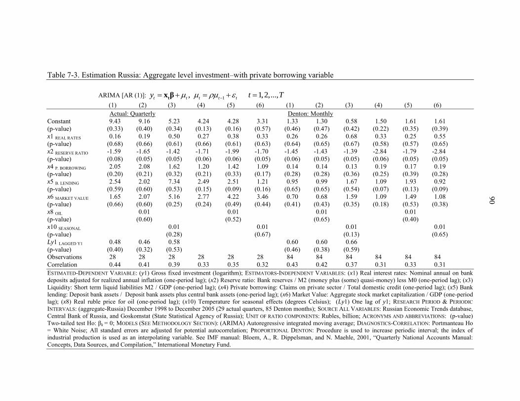
90
Table 7-3. Estimation Russia: Aggregate level investment–with private borrowing variable ARIMA [AR (1)]: 1, 1,2,..., t t t t ty t T tx β (1) (2) (3) (4) (5) (6) (1) (2) (3) (4) (5) (6) Actual: Quarterly Denton: Monthly Constant 9.43 9.16 5.23 4.24 4.28 3.31 1.33 1.30 0.58 1.50 1.61 1.61 (p-value) (0.33) (0.40) (0.34) (0.13) (0.16) (0.57) (0.46) (0.47) (0.42) (0.22) (0.35) (0.39) x1 REAL RATES 0.16 0.19 0.50 0.27 0.38 0.33 0.26 0.26 0.68 0.33 0.25 0.55 (p-value) (0.68) (0.66) (0.61) (0.66) (0.61) (0.63) (0.64) (0.65) (0.67) (0.58) (0.57) (0.65) x2 RESERVE RATIO -1.59 -1.65 -1.42 -1.71 -1.99 -1.70 -1.45 -1.43 -1.39 -2.84 -1.79 -2.84 (p-value) (0.08) (0.05) (0.05) (0.06) (0.06) (0.05) (0.06) (0.05) (0.05) (0.06) (0.05) (0.05) x4 P. BORROWING 2.05 2.08 1.62 1.20 1.42 1.09 0.14 0.14 0.13 0.19 0.17 0.19 (p-value) (0.20) (0.21) (0.32) (0.21) (0.33) (0.17) (0.28) (0.28) (0.36) (0.25) (0.39) (0.28) x5 B. LENDING 2.54 2.02 7.34 2.49 2.51 1.21 0.95 0.99 1.67 1.09 1.93 0.92 (p-value) (0.59) (0.60) (0.53) (0.15) (0.09) (0.16) (0.65) (0.65) (0.54) (0.07) (0.13) (0.09) x6 MARKET VALUE 1.65 2.07 5.16 2.77 4.22 3.46 0.70 0.68 1.59 1.09 1.49 1.08 (p-value) (0.66) (0.60) (0.25) (0.24) (0.49) (0.44) (0.41) (0.43) (0.35) (0.18) (0.53) (0.38) x8 OIL 0.01 0.01 0.01 0.01 (p-value) (0.60) (0.52) (0.65) (0.40) x10 SEASONAL 0.01 0.01 0.01 0.01 (p-value) (0.28) (0.67) (0.13) (0.65) Ly1 LAGGED Y1 0.48 0.46 0.58 0.60 0.60 0.66 (p-value) (0.40) (0.32) (0.53) (0.46) (0.38) (0.59) Observations 28 28 28 28 28 28 84 84 84 84 84 84 Correlation 0.44 0.41 0.39 0.33 0.35 0.32 0.43 0.42 0.37 0.31 0.33 0.31 ESTIMATED-DEPENDENT VARIABLE: (y1) Gross fixed investment (logarithm); ESTIMATORS-INDEPENDENT VARIABLES: (x1) Real interest rates: Nominal annual on bank deposits adjusted for realized annual inflation (one-period lag); (x2) Reserve ratio: Bank reserves / M2 (money plus (some) quasi-money) less M0 (one-period lag); (x3) Liquidity: Short term liquid liabilities M2 / GDP (one-period lag); (x4) Private borrowing: Claims on private sector / Total domestic credit (one-period lag); (x5) Bank lending: Deposit bank assets / Deposit bank assets plus central bank assets (one-period lag); (x6) Market Value: Aggregate stock market capitalization / GDP (one-period lag); (x8) Real ruble price for oil (one-period lag); (x10) Temperature for seasonal effects (degrees Celsius); (Ly1) One lag of y1; RESEARCH PERIOD & PERIODIC INTERVALS: (aggregate-Russia) December 1998 to December 2005 (29 actual quarters, 85 Denton months); SOURCE ALL VARIABLES: Russian Economic Trends database, Central Bank of Russia, and Goskomstat (State Statistical Agency of Russia); UNIT OF RATIO COMPONENTS: Rubles, billion; ACRONYMS AND ABBREVIATIONS: (p-value) Two-tailed test Ho: βk = 0; MODELS (SEE METHODOLOGY SECTION): (ARIMA) Autoregressive integrated moving average; DIAGNOSTICS-CORRELATION: Portmanteau Ho = White Noise; All standard errors are adjusted for potential autocorrelation; PROPORTIONAL DENTON: Procedure is used to increase periodic interval; the index of industrial production is used as an interpolating variable. See IMF manual: Bloem, A., R. Dippelsman, and N. Maehle, 2001, “Quarterly National Accounts Manual: Concepts, Data Sources, and Compilation,” International Monetary Fund.

91
Table 7-4. Descriptive statistics and correlation - Russia: Large firm level y1 Ly1 x1 x2 x3 x4 x5 x6 x7 x8 x9 x10
DESCRIPTIVE STATISTICS Mean 0.10 0.10 -0.10 0.34 0.67 1.35 0.64 0.08 1.33 693.03 23.78 4.40 Median 0.05 0.05 -0.08 0.34 0.64 1.33 0.64 0.08 0.91 684.13 6.25 1.21 Maximum 12.66 12.66 0.00 0.46 0.97 1.89 0.68 0.14 10.77 1534.95 422.84 20.76 Minimum -0.92 -0.92 -0.65 0.22 0.43 0.83 0.62 0.02 0.04 50.24 0.01 -10.38 St. Deviation 0.52 0.53 0.10 0.06 0.14 0.22 0.01 0.03 1.34 280.07 47.12 9.87 Observations 988 948 988 988 988 988 988 988 988 988 948 988 CORRELATIONS y1 INVESTMENT 1.00 Ly1 LAGGED Y1 0.14 1.00 x1 REAL RATES -0.07 -0.01 1.00 x2 RESERVE RATIO -0.01 -0.04 -0.28 1.00 x3 LIQUIDITY -0.07 -0.12 0.32 -0.55 1.00 x4 P. BORROWING 0.06 0.03 0.19 -0.36 0.76 1.00 x5 B. LENDING -0.14 -0.10 0.32 -0.14 0.45 -0.27 1.00 x6 MARKET VALUE -0.08 -0.16 0.39 -0.36 0.69 0.30 0.48 1.00 x7 F. CHARACTERISTIC 0.07 0.04 0.02 -0.05 0.08 0.06 0.02 0.06 1.00 x8 OIL -0.07 -0.12 0.31 -0.16 0.65 0.62 0.17 0.67 0.08 1.00 x9 A. PRINCIPLE 0.03 0.03 0.10 -0.48 0.22 0.19 0.04 0.18 -0.04 0.26 1.00 x10 SEASONAL 0.02 -0.11 -0.23 0.13 0.13 -0.43 -0.19 0.13 -0.01 -0.07 -0.05 1.00 VARIABLES: (y1) Gross fixed investment (scaled by one-period lagged “PP&E” assets); (Ly1) One lag of y1; (x1) Real interest rates: Nominal annual on bank deposits adjusted for realized annual inflation (one-period lag); (x2) Reserve ratio: Bank reserves / M2 (money plus (some)quasi-money) less M0 (one-period lag); (x3) Liquidity: Short term liquid liabilities M2 / GDP (one-period lag); (x4) Private borrowing: Claims on private sector / Total domestic credit (one-period lag); (x5) Bank lending: Deposit bank assets / Deposit bank assets plus central bank assets (one-period lag); (x6) Market Value: Aggregate stock market capitalization / GDP (one-period lag); (x7) Firm characteristic: Total revenue / Total assets; (x8) Real ruble price for oil (one-period lag); (x9) Acceleration principle: One lag of revenue; (x10) Temperature for seasonal effects (degrees Celsius); RESEARCH PERIOD & PERIODIC INTERVALS: (Russia-unbalanced) December 1998 to December 2005 (29 to 17 Denton quarters); FIRM COUNT (Russia): 40; SOURCE DEPENDENT VARIABLES: Worldscope, Global Reports, and Company Financials; SOURCE INDEPENDENT VARIABLES: Russian Economic Trends database, Central Bank of Russia, and Goskomstat (State Statistical Agency of Russia); UNIT OF INVESTMENT AND RATIO COMPONENTS: Rubles, billion; RUSSIA-UNBALANCED LARGE FIRM PANELS: 8 years (29 Denton interpolated quarters): 17 companies; 7 years (25 Denton interpolated quarters): 12 companies; 6 years (21 Denton interpolated quarters): 2 companies; 5 years (17 Denton interpolated quarters): 9 companies

92
Table 7-5. Estimation - Russia: Large firm level investment–with liquidity variable GLS [Random Effects]: firm 1,2,..., ; 1,2,..., th
it i ity i N t T it
x β (1) (2) (3) (4) (5) (6) (7) (8) (9) (10)
Denton: Quarterly Constant 1.67 1.77 1.64 1.74 0.01 1.97 2.00 2.02 2.03 2.00 (p-value) (0.00) (0.00) (0.00) (0.00) (0.03) (0.00) (0.00) (0.00) (0.00) (0.00) x1 REAL RATES -0.01 -0.01 -0.01 -0.01 -0.01 -0.03 -0.01 -0.03 -0.05 -0.03 (p-value) (0.60) (0.64) (0.67) (0.66) (0.63) (0.50) (0.56) (0.47) (0.58) (0.51) x2 RESERVE RATIO -0.48 -0.51 -0.50 -0.48 -0.49 -0.46 -0.47 -0.43 -0.46 -0.46 (p-value) (0.01) (0.00) (0.01) (0.00) (0.02) (0.03) (0.01) (0.00) (0.00) (0.04) x3 LIQUIDITY -0.29 -0.18 -0.29 -0.31 -0.29 -0.35 -0.26 -0.34 -0.38 -0.36 (p-value) (0.01) (0.03) (0.00) (0.01) (0.01) (0.00) (0.00) (0.02) (0.02) (0.02) x5 B. LENDING -2.05 -2.21 -1.98 -2.15 -2.09 -2.52 -2.56 -2.63 -2.64 -2.56 (p-value) (0.02) (0.00) (0.01) (0.01) (0.01) (0.00) (0.00) (0.02) (0.01) (0.01) x6 MARKET VALUE 0.91 0.89 0.87 1.02 0.94 1.32 1.21 1.34 1.44 1.35 (p-value) (0.01) (0.01) (0.01) (0.00) (0.01) (0.00) (0.00) (0.01) (0.00) (0.01) x7 F. CHARACTERISTIC 0.01 0.02 (p-value) (0.61) (0.42) x8 OIL 0.01 0.01 (p-value) (0.09) (0.08) x9 A. PRINCIPLE -0.01 -0.01 (p-value) (0.68) (0.58) x10 SEASONAL 0.01 0.01 (p-value) (0.62) (0.52) Ly1 LAGGED Y1 0.01 0.01 0.01 0.01 0.01 (p-value) (0.85) (0.65) (0.72) (0.65) (0.93) Observations 908 908 908 908 908 948 948 948 948 948 CCN collinearity 6.02 6.80 6.05 6.03 6.10 5.88 6.74 5.93 5.90 5.97 ESTIMATED-DEPENDENT VARIABLE: (y1) Gross fixed investment (scaled by one-period lagged “PP&E”
assets); ESTIMATORS-INDEPENDENT VARIABLES: (x1) Real interest rates: Nominal annual on bank deposits adjusted for realized annual inflation (one-period lag); (x2) Reserve ratio: Bank reserves / M2 (money plus (some) quasi-money) less M0 (one-period lag); (x3) Liquidity: Short term liquid liabilities M2 / GDP (one-period lag); (x4) Private borrowing: Claims on private sector / Total domestic credit (one-period lag); (x5) Bank lending: Deposit bank assets / Deposit bank assets plus central bank assets (one-period lag); (x6) Market Value: Aggregate stock market capitalization / GDP (one-period lag); (x7) Firm characteristic: Total revenue / Total assets (one-period lag); (x8) Real ruble price for oil (one-period lag); (x9) Acceleration principle: One lag of revenue; (x10) Temperature for seasonal effects (degrees Celsius); (Ly1) One lag of y1; RESEARCH PERIOD & PERIODIC INTERVALS: (Russia-unbalanced) December 1998 to December 2005 (29 to 17 Denton quarters (Observations per group of 40 firms: 15 min 27 max for dynamic models and 16 min 28 max for static models); FIRM COUNT (Russia): 40; SOURCE DEPENDENT VARIABLES: Worldscope, Global Reports, and Company Financials; SOURCE INDEPENDENT VARIABLES: Russian Economic Trends database, Central Bank of Russia, and Goskomstat (State Statistical Agency of Russia); UNIT OF RATIO COMPONENTS: Rubles, billion; ACRONYMS AND ABBREVIATIONS: (CCN) Collinearity Condition Number; (p-value) Two-tailed test Ho: βk = 0; MODELS (SEE METHODOLOGY SECTION): (GLS) Generalized Least Squares; DIAGNOSTICS-CORRELATION: (CCN) Collinearity Condition Number 1 ≤ Best CCN ≤ 20; All standard errors are adjusted for potential panel heteroskedasticity and
autocorrelation; PROPORTIONAL DENTON: Procedure is used to increase periodic interval; the index of industrial production is used as an interpolating variable. See IMF manual: Bloem, A., R. Dippelsman, and N. Maehle, 2001, “Quarterly National Accounts Manual: Concepts, Data Sources, and Compilation,”
International Monetary Fund; RUSSIA-UNBALANCED LARGE FIRM PANELS: 8 years (29 Denton interpolated quarters): 17 companies; 7 years (25 Denton interpolated quarters): 12 companies; 6 years (21 Denton interpolated quarters): 2 companies; 5 years (17 Denton interpolated quarters): 9 companies.

93
93
Table 7-6. Estimation – Russia: Large firm level investment–with private borrowing variable
GLS [Random Effects]: firm 1,2,..., ; 1,2,..., th
it i ity i N t T it
x β (1) (2) (3) (4) (5) (6) (7) (8) (9) (10)
Denton: Quarterly Constant 1.52 1.39 1.48 1.55 1.54 1.62 1.51 1.86 1.66 1.63 (p-value) (0.00) (0.00) (0.00) (0.00) (0.00) (0.00) (0.00) (0.00) (0.00) (0.00) x1 REAL RATES -0.05 -0.03 -0.05 -0.04 -0.06 -0.03 -0.03 -0.01 -0.05 -0.03 (p-value) (0.61) (0.65) (0.63) (0.66) (0.57) (0.50) (0.56) (0.65) (0.36) (0.48) x2 RESERVE RATIO -0.30 -0.36 -0.30 -0.28 -0.30 -0.25 -0.27 -0.25 -0.26 -0.25 (p-value) (0.05) (0.02) (0.00) (0.04) (0.01) (0.01) (0.00) (0.01) (0.02) (0.01) x4 P. BORROWING 0.01 0.11 0.01 0.02 0.01 0.04 0.13 0.01 0.04 0.05 (p-value) (0.43) (0.10) (0.69) (0.53) (0.52) (0.15) (0.21) (0.58) (0.23) (0.10) x5 B. LENDING -1.01 -1.98 -2.05 -2.18 -2.16 -2.39 -2.27 -2.71 -2.48 -2.41 (p-value) (0.03) (0.00) (0.02) (0.00) (0.01) (0.02) (0.00) (0.02) (0.00) (0.01) x6 MARKET VALUE 0.17 0.40 0.20 0.12 0.13 0.02 0.52 0.16 0.02 0.02 (p-value) (0.42) (0.10) (0.50) (0.59) (0.53) (0.62) (0.04) (0.61) (0.61) (0.60) x7 F. CHARACTERISTIC 0.01 0.02 (p-value) (0.65) (0.54) x8 OIL 0.01 0.01 (p-value) (0.10) (0.09) x9 A. PRINCIPLE -0.01 -0.01 (p-value) (0.53) (0.26) x10 SEASONAL 0.01 0.01 (p-value) (0.40) (0.38) Ly1 LAGGED Y1 0.01 0.01 0.01 0.01 0.01 (p-value) (0.50) (0.64) (0.44) (0.69) (0.62) Observations 908 908 908 908 908 948 948 948 948 948 CCN collinearity 2.80 3.61 5.38 2.80 2.85 2.90 3.81 5.14 2.91 2.96 ESTIMATED-DEPENDENT VARIABLE: (y1) Gross fixed investment (scaled by one-period lagged “PP&E”
assets); ESTIMATORS-INDEPENDENT VARIABLES: (x1) Real interest rates: Nominal annual on bank deposits adjusted for realized annual inflation (one-period lag); (x2) Reserve ratio: Bank reserves / M2 (money plus (some) quasi-money) less M0 (one-period lag); (x3) Liquidity: Short term liquid liabilities M2 / GDP (one-period lag); (x4) Private borrowing: Claims on private sector / Total domestic credit (one-period lag); (x5) Bank lending: Deposit bank assets / Deposit bank assets plus central bank assets (one-period lag); (x6) Market Value: Aggregate stock market capitalization / GDP (one-period lag); (x7) Firm characteristic: Total revenue / Total assets (one-period lag); (x8) Real ruble price for oil (one-period lag); (x9) Acceleration principle: One lag of revenue; (x10) Temperature for seasonal effects (degrees Celsius); (Ly1) One lag of y1; RESEARCH PERIOD & PERIODIC INTERVALS: (Russia-unbalanced) December 1998 to December 2005 (29 to 17 Denton quarters (Observations per group of 40 firms: 15 min 27 max for dynamic models and 16 min 28 max for static models); FIRM COUNT (Russia): 40; SOURCE DEPENDENT VARIABLES: Worldscope, Global Reports, and Company Financials; SOURCE INDEPENDENT VARIABLES: Russian Economic Trends database, Central Bank of Russia, and Goskomstat (State Statistical Agency of Russia); UNIT OF RATIO COMPONENTS: Rubles, billion; ACRONYMS AND ABBREVIATIONS: (CCN) Collinearity Condition Number; (p-value) Two-tailed test Ho: βk = 0; MODELS (SEE METHODOLOGY SECTION): (GLS) Generalized Least Squares; DIAGNOSTICS-CORRELATION: (CCN) Collinearity Condition Number 1 ≤ Best CCN ≤ 20; All standard errors are adjusted for potential panel heteroskedasticity and autocorrelation; PROPORTIONAL DENTON: Procedure is used to increase periodic interval; the index of industrial production is used as an interpolating variable. See IMF manual: Bloem, A., R. Dippelsman, and N. Maehle, 2001, “Quarterly National Accounts Manual: Concepts, Data Sources, and Compilation,”
International Monetary Fund; RUSSIA-UNBALANCED LARGE FIRM PANELS: 8 years (29 Denton interpolated quarters): 17 companies; 7 years (25 Denton interpolated quarters): 12 companies; 6 years (21 Denton interpolated quarters): 2 companies; 5 years (17 Denton interpolated quarters): 9 companies.

94
Table 7-7. Descriptive statistics and correlation USA: Aggregate level y1 Ly1 x1 x2 x3 x4 x5 x6 x8 DESCRIPTIVE STATISTICS Mean 7.40 7.39 0.01 0.01 0.50 0.28 0.90 1.32 10.9 Median 7.38 7.38 0.01 0.01 0.51 0.30 0.90 1.33 9.5 Maximum 7.71 7.68 0.04 0.02 0.54 0.34 0.91 1.62 19.4 Minimum 7.14 7.14 -0.02 0.01 0.46 0.23 0.89 0.96 6.6 St. Deviation 0.13 0.13 0.01 0.01 0.02 0.03 0.01 0.17 3.6 Observations 37 36 37 37 37 37 37 37 37 CORRELATIONS y1 INVESTMENT 1.00 Ly1 LAGGED Y1 0.99 1.00 x1 REAL RATES -0.66 -0.64 1.00 x2 RESERVE RATIO -0.27 -0.30 0.41 1.00 x3 LIQUIDITY 0.59 0.57 -0.61 -0.56 1.00 x4 P. BORROWING -0.66 -0.63 0.60 0.36 -0.87 1.00 x5 B. LENDING 0.44 0.56 -0.26 -0.47 0.30 -0.39 1.00 x6 MARKET VALUE 0.10 0.07 0.65 0.21 -0.62 0.47 -0.10 1.00 x8 OIL 0.56 0.53 -0.66 -0.37 0.76 -0.66 0.17 -0.44 1.00 VARIABLES: (y1) Gross fixed investment (logarithm); (Ly1) One lag of y1; (x1) Real interest rates: Nominal annual on bank deposits adjusted for realized annual inflation (one-period lag); (x2) Reserve ratio: Bank reserves / M2 less M0 (one-period lag); (x3) Liquidity: Short term liquid liabilities M2 / GDP (one-period lag); (x4) Private borrowing: Claims on private sector / Total domestic credit (one-period lag); (x5) Bank lending: Deposit bank assets / Deposit bank assets plus central bank assets (one-period lag); (x6) Market Value: Aggregate stock market capitalization / GDP (one-period lag); (x8) Real dollar price for oil (one-period lag); RESEARCH PERIOD & PERIODIC INTERVALS: (aggregate-USA) December 1996 to December 2005 (37 actual quarters, 109 Denton months); SOURCE ALL VARIABLES: (USA) Federal Reserve, U.S. Department of Commerce: Bureau of Economic Analysis, and Bureau of Labor Statistics (BLS); UNIT OF INVESTMENT AND RATIO COMPONENTS: Dollars, billion

95
95
Table 7-8. Estimation USA: Aggregate level investment–with liquidity variable ARIMA [AR (1)]: 1, 1,2,..., t t t t ty t T tx β (1) (2) (3) (4) (1) (2) (3) (4) Actual: Quarterly Denton: Monthly Constant 0.64 0.49 5.21 5.38 0.36 0.32 8.01 9.87 (p-value) (0.48) (0.59) (0.15) (0.14) (0.09) (0.14) (0.14) (0.15) x1 REAL RATES -0.48 -0.37 -6.70 -6.34 -0.09 -0.12 -7.63 -7.31 (p-value) (0.28) (0.39) (0.10) (0.21) (0.43) (0.33) (0.11) (0.25) x2 RESERVE RATIO 1.53 1.73 10.78 10.77 1.17 1.20 11.26 10.53 (p-value) (0.18) (0.16) (0.07) (0.09) (0.19) (0.19) (0.12) (0.11) x3 LIQUIDITY 0.49 0.57 0.66 0.40 0.01 0.02 0.05 0.20 (p-value) (0.21) (0.11) (0.69) (0.80) (0.41) (0.23) (0.66) (0.30) x5 B. LENDING 0.73 0.48 12.71 13.00 0.48 0.39 7.24 7.39 (p-value) (0.39) (0.50) (0.20) (0.13) (0.07) (0.16) (0.23) (0.11) x6 MARKET VALUE 0.04 0.04 0.47 0.46 0.01 0.01 0.16 0.16 (p-value) (0.08) (0.09) (0.12) (0.13) (0.21) (0.37) (0.15) (0.13) x8 OIL 0.01 0.01 0.01 0.01 (p-value) (0.08) (0.33) (0.24) (0.21) Ly1 LAGGED Y1 1.04 1.03 1.01 1.01 (p-value) (0.00) (0.00) (0.00) (0.00) Observations 36 36 36 36 108 108 108 108 Correlation 0.28 0.16 0.16 0.11 0.33 0.35 0.17 0.12 ESTIMATED-DEPENDENT VARIABLE: (y1) Gross fixed investment (logarithm); ESTIMATORS-INDEPENDENT VARIABLES: (x1) Real interest rates: Nominal annual on bank deposits adjusted for realized annual inflation (one-period lag); (x2) Reserve ratio: Bank reserves / M2 less M0 (one-period lag); (x3) Liquidity: Short term liquid liabilities M2 / GDP (one-period lag); (x4) Private borrowing: Claims on private sector / Total domestic credit (one-period lag); (x5) Bank lending: Deposit bank assets / Deposit bank assets plus central bank assets (one-period lag); (x6) Market Value: Aggregate stock market capitalization / GDP (one-period lag); (x8) Real dollar price for oil (one-period lag); (Ly1) One lag of y1; RESEARCH PERIOD & PERIODIC INTERVALS: (aggregate-USA) December 1996 to December 2005 (37 actual quarters, 109 Denton months); SOURCE ALL VARIABLES: (USA) Federal Reserve, U.S. Department of Commerce: Bureau of Economic Analysis, and Bureau of Labor Statistics (BLS); UNIT OF RATIO COMPONENTS: Dollars, billion; ACRONYMS AND ABBREVIATIONS: (p-value) Two-tailed test Ho: βk = 0; MODELS (SEE METHODOLOGY SECTION): (ARIMA) Autoregressive integrated moving average; DIAGNOSTICS-CORRELATION: Portmanteau Ho = White Noise; All standard errors are adjusted for potential autocorrelation; PROPORTIONAL DENTON: Procedure is used to increase periodic interval; the index of industrial production is used as an interpolating variable. See IMF manual: Bloem, A., R. Dippelsman, and N. Maehle, 2001, “Quarterly National Accounts
Manual: Concepts, Data Sources, and Compilation,” International Monetary Fund.

96
96
Table 7-9. Estimation - USA: Aggregate level investment–with private borrowing variable
ARIMA [AR (1)]: 1, 1,2,..., t t t t ty t T tx β (1) (2) (3) (4) (1) (2) (3) (4) Actual: Quarterly Denton: Monthly Constant 1.54 1.57 4.47 5.38 0.50 0.45 0.92 1.31 (p-value) (0.08) (0.02) (0.08) (0.09) (0.08) (0.09) (0.57) (0.43) x1 REAL RATES -0.65 -0.66 -0.44 -0.29 -0.07 -0.06 -0.03 -0.14 (p-value) (0.13) (0.12) (0.65) (0.72) (0.49) (0.58) (0.65) (0.74) x2 RESERVE RATIO 3.34 3.34 2.89 1.94 1.19 1.23 2.32 1.91 (p-value) (0.22) (0.24) (0.46) (0.63) (0.31) (0.28) (0.37) (0.47) x4 P. BORROWING -0.67 -0.68 -3.94 -4.18 -0.14 -0.12 -1.79 -2.91 (p-value) (0.01) (0.21) (0.01) (0.00) (0.04) (0.11) (0.03) (0.00) x5 B. LENDING 1.11 1.13 3.96 3.11 0.47 0.43 1.56 1.20 (p-value) (0.10) (0.10) (0.13) (0.22) (0.09) (0.14) (0.21) (0.25) x6 MARKET VALUE 0.02 0.02 0.31 0.31 0.01 0.00 0.12 0.12 (p-value) (0.56) (0.56) (0.09) (0.08) (0.60) (0.66) (0.10) (0.11) x8 OIL 0.01 0.01 0.01 0.01 (p-value) (0.67) (0.41) (0.69) (0.65) Ly1 LAGGED Y1 0.94 0.94 0.99 0.99 (p-value) (0.00) (0.00) (0.00) (0.00) Observations 36 36 36 36 108 108 108 108 Correlation 0.24 0.24 0.18 0.11 0.26 0.29 0.17 0.12 ESTIMATED-DEPENDENT VARIABLE: (y1) Gross fixed investment (logarithm); ESTIMATORS-INDEPENDENT VARIABLES: (x1) Real interest rates: Nominal annual on bank deposits adjusted for realized annual inflation (one-period lag); (x2) Reserve ratio: Bank reserves / M2 less M0 (one-period lag); (x3) Liquidity: Short term liquid liabilities M2 / GDP (one-period lag); (x4) Private borrowing: Claims on private sector / Total domestic credit (one-period lag); (x5) Bank lending: Deposit bank assets / Deposit bank assets plus central bank assets (one-period lag); (x6) Market Value: Aggregate stock market capitalization / GDP (one-period lag); (x8) Real dollar price for oil (one-period lag); (Ly1) One lag of y1; RESEARCH PERIOD & PERIODIC INTERVALS: (aggregate-USA) December 1996 to December 2005 (37 actual quarters, 109 Denton months); SOURCE ALL VARIABLES: (USA) Federal Reserve, U.S. Department of Commerce: Bureau of Economic Analysis, and Bureau of Labor Statistics (BLS); UNIT OF RATIO COMPONENTS: Dollars, billion; ACRONYMS AND ABBREVIATIONS: (p-value) Two-tailed test Ho: βk = 0; MODELS (SEE METHODOLOGY SECTION): (ARIMA) Autoregressive integrated moving average; DIAGNOSTICS-CORRELATION: Portmanteau Ho = White Noise; All standard errors are adjusted for potential autocorrelation; PROPORTIONAL DENTON: Procedure is used to increase periodic interval; the index of industrial production is used as an interpolating variable. See IMF manual: Bloem, A., R. Dippelsman, and N. Maehle, 2001, “Quarterly National Accounts
Manual: Concepts, Data Sources, and Compilation,” International Monetary Fund.

97
Table 7-10. Descriptive statistics and correlation USA: Large firm level y1 Ly1 x1 x2 x3 x4 x5 x6 x7 x8 x9 DESCRIPTIVE STATISTICS Mean 0.03 0.03 0.01 0.01 0.50 0.28 0.90 1.32 1.08 10.90 3915.65 Median 0.01 0.01 0.00 0.01 0.51 0.30 0.90 1.33 0.87 9.55 2330.88 Maximum 6.42 6.42 0.04 0.02 0.54 0.34 0.91 1.62 6.43 19.46 25709.34 Minimum -0.84 -0.84 -0.02 0.01 0.46 0.23 0.89 0.96 0.06 6.60 230.41 St. Deviation 0.34 0.34 0.01 0.00 0.02 0.03 0.00 0.17 0.78 3.55 4172.27 Observations 1036 1008 1036 1036 1036 1036 1036 1036 1036 1036 1008 CORRELATIONS y1 INVESTMENT 1.00 Ly1 LAGGED Y1 -0.10 1.00 x1 REAL RATES 0.06 0.06 1.00 x2 RESERVE RATIO 0.04 0.03 0.42 1.00 x3 LIQUIDITY -0.06 -0.06 -0.62 -0.58 1.00 x4 P. BORROWING 0.06 0.05 0.61 0.38 -0.86 1.00 x5 B. LENDING 0.01 0.03 -0.25 -0.50 0.27 -0.35 1.00 x6 MARKET VALUE 0.05 0.06 0.68 0.20 -0.69 0.55 -0.15 1.00 x7 F. CHARACTERISTIC 0.21 0.07 0.01 0.02 -0.02 -0.01 -0.01 0.03 1.00 x8 OIL -0.05 -0.04 -0.66 -0.39 0.65 -0.65 0.14 -0.50 -0.01 1.00 x9 A. PRINCIPLE 0.02 0.01 -0.14 -0.08 0.13 -0.16 0.06 -0.06 -0.04 0.11 1.00 VARIABLES: (y1) Gross fixed investment (scaled by one-period lagged “PP&E” assets); (Ly1) One lag of y1; (x1) Real interest rates: Nominal annual on bank deposits adjusted for realized annual inflation (one-period lag); (x2) Reserve ratio: Bank reserves / M2 less M0 (one-period lag); (x3) Liquidity: Short term liquid liabilities M2 / GDP (one-period lag); (x4) Private borrowing: Claims on private sector / Total domestic credit (one-period lag); (x5) Bank lending: Deposit bank assets / Deposit bank assets plus central bank assets (one-period lag); (x6) Market Value: Aggregate stock market capitalization / GDP (one-period lag); (x7) Firm characteristic: Total revenue / Total assets; (x8) Real dollar price for oil (one-period lag); (x9) Acceleration principle: One lag of revenue RESEARCH PERIOD & PERIODIC INTERVALS: (USA-balanced panels) December 1996 to December 2005 (37 actual quarters, 37 Denton quarters); FIRM COUNT (USA): 28; SOURCE DEPENDENT VARIABLES: (large firms-USA): Worldscope, SEC, and Company Financials; SOURCE INDEPENDENT VARIABLES: (USA) Federal Reserve, U.S. Department of Commerce: Bureau of Economic Analysis, and Bureau of Labor Statistics (BLS); UNIT OF INVESTMENT AND RATIO COMPONENTS: Dollars, billion

98
Table 7-11. Estimation USA: Large firm level investment–with liquidity variable GLS [Random Effects]: firm 1,2,..., ; 1,2,..., th
it i ity i N t T it
x β (1) (2) (3) (4) (5) (6) (7) (8) (1) (2) (3) (4) (5) (6) (7) (8) Actual: Quarterly Denton: Quarterly Constant 0.43 0.31 0.76 0.41 1.26 1.22 2.25 1.28 0.03 0.07 0.16 0.03 0.23 0.22 0.49 0.22 (p-value) (0.47) (0.61) (0.34) (0.50) (0.40) (0.51) (0.50) (0.20) (0.60) (0.67) (0.67) (0.60) (0.23) (0.25) (0.16) (0.24) x1 REAL RATES -0.07 -0.02 -0.09 -0.08 -0.21 -0.16 -0.06 -0.21 -0.64 -0.69 -0.52 -0.64 -0.47 -0.47 -0.40 -0.47 (p-value) (0.69) (0.61) (0.68) (0.66) (0.33) (0.47) (0.65) (0.34) (0.60) (0.65) (0.66) (0.52) (0.43) (0.42) (0.63) (0.39) x2 RESERVE RATIO -0.50 -0.66 -0.13 -0.48 -0.46 -0.44 -1.04 -0.48 -1.50 -1.69 -1.85 -1.50 -0.37 -0.39 -0.79 -0.37 (p-value) (0.61) (0.50) (0.61) (0.63) (0.55) (0.57) (0.37) (0.54) (0.58) (0.50) (0.67) (0.69) (0.52) (0.50) (0.25) (0.52) x3 LIQUIDITY 0.44 0.39 0.51 0.46 0.19 0.15 0.25 0.22 0.51 0.48 0.41 0.51 0.23 0.23 0.27 0.34 (p-value) (0.09) (0.08) (0.09) (0.09) (0.25) (0.38) (0.33) (0.21) (0.10) (0.09) (0.13) (0.10) (0.20) (0.40) (0.27) (0.20) x5 B. LENDING 0.77 0.62 1.15 0.75 1.51 1.45 2.61 1.54 0.41 0.29 0.42 0.41 0.49 0.49 0.67 0.49 (p-value) (0.21) (0.31) (0.15) (0.22) (0.12) (0.06) (0.09) (0.10) (0.12) (0.28) (0.29) (0.12) (0.11) (0.07) (0.06) (0.11) x6 MARKET VALUE 0.01 0.01 0.01 0.01 0.01 0.01 0.03 0.02 0.01 0.01 0.01 0.01 0.02 0.02 0.02 0.02 (p-value) (0.69) (0.61) (0.58) (0.62) (0.66) (0.66) (0.60) (0.58) (0.47) (0.53) (0.44) (0.47) (0.61) (0.50) (0.55) (0.50) x7 F. CHARACTERISTIC 0.02 0.02 0.02 0.02 (p-value) (0.00) (0.01) (0.01) (0.01) x8 OIL 0.01 0.01 0.01 0.01 (p-value) (0.18) (0.34) (0.09) (0.36) x9 A. PRINCIPLE 2.83 1.93 2.99 2.00 (p-value) (0.10) (0.19) (0.09) (0.30) Ly1 LAGGED Y1 0.24 0.24 0.35 0.26 0.40 0.41 0.21 0.40 (p-value) (0.00) (0.00) (0.00) (0.00) (0.00) (0.00) (0.00) (0.00) Observations 980 980 980 980 1008 1008 1008 1008 980 980 980 980 1008 1008 1008 1008 CCN collinearity 8.28 9.06 8.28 8.31 7.36 7.36 6.71 6.74 8.31 9.09 6.76 6.76 7.37 7.37 6.76 6.76 ESTIMATED-DEPENDENT VARIABLE: (y1) Gross fixed investment (scaled by one-period lagged “PP&E” assets); ESTIMATORS-INDEPENDENT VARIABLES: (x1) Real interest rates: Nominal annual on bank deposits adjusted for realized annual inflation (one-period lag); (x2) Reserve ratio: Bank reserves / M2 less M0 (one-period lag); (x3) Liquidity: Short term liquid liabilities M2 / GDP (one-period lag); (x4) Private borrowing: Claims on private sector / Total domestic credit (one-period lag); (x5) Bank lending: Deposit bank assets / Deposit bank assets plus central bank assets (one-period lag); (x6) Market Value: Aggregate stock market capitalization / GDP (one-period lag); (x7) Firm characteristic: Total revenue / Total assets (one-period lag); (x8) Real dollar price for oil (one-period lag); (x9) Acceleration principle: One lag of revenue; (Ly1) One lag of y1; RESEARCH PERIOD & PERIODIC INTERVALS: (USA-balanced panels) December 1996 to December 2005 (37 actual quarters, 37 Denton quarters); FIRM COUNT (USA): 28; SOURCE DEPENDENT VARIABLES: (large firms-USA): Worldscope, SEC, and Company Financials; SOURCE INDEPENDENT VARIABLES: (USA) Federal Reserve, U.S. Department of Commerce: Bureau of Economic Analysis, and Bureau of Labor Statistics (BLS); UNIT OF RATIO COMPONENTS: Dollars, billion; ACRONYMS AND ABBREVIATIONS: (CCN) Collinearity Condition Number; (p-value) Two-tailed test Ho: βk = 0; MODELS (SEE METHODOLOGY SECTION): (GLS) Generalized Least Squares; DIAGNOSTICS-CORRELATION: (CCN) Collinearity Condition Number 1 ≤ Best CCN ≤ 20; All standard errors are adjusted for potential panel
heteroskedasticity and autocorrelation; PROPORTIONAL DENTON: Procedure is used to increase periodic interval; the index of industrial production is used as an interpolating variable. See IMF manual: Bloem, A., R. Dippelsman, and N. Maehle, 2001, “Quarterly National Accounts Manual: Concepts, Data Sources, and Compilation,” International Monetary Fund.
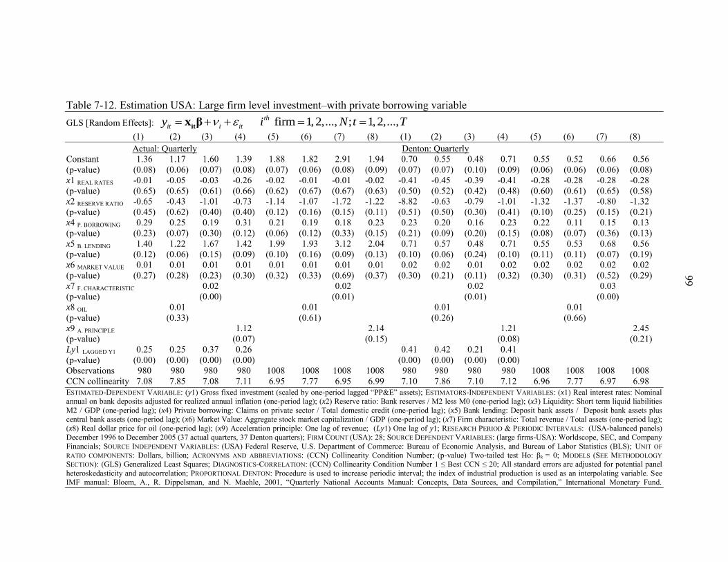
99
Table 7-12. Estimation USA: Large firm level investment–with private borrowing variable GLS [Random Effects]: firm 1,2,..., ; 1,2,..., th
it i ity i N t T it
x β (1) (2) (3) (4) (5) (6) (7) (8) (1) (2) (3) (4) (5) (6) (7) (8) Actual: Quarterly Denton: Quarterly Constant 1.36 1.17 1.60 1.39 1.88 1.82 2.91 1.94 0.70 0.55 0.48 0.71 0.55 0.52 0.66 0.56 (p-value) (0.08) (0.06) (0.07) (0.08) (0.07) (0.06) (0.08) (0.09) (0.07) (0.07) (0.10) (0.09) (0.06) (0.06) (0.06) (0.08) x1 REAL RATES -0.01 -0.05 -0.03 -0.26 -0.02 -0.01 -0.01 -0.02 -0.41 -0.45 -0.39 -0.41 -0.28 -0.28 -0.28 -0.28 (p-value) (0.65) (0.65) (0.61) (0.66) (0.62) (0.67) (0.67) (0.63) (0.50) (0.52) (0.42) (0.48) (0.60) (0.61) (0.65) (0.58) x2 RESERVE RATIO -0.65 -0.43 -1.01 -0.73 -1.14 -1.07 -1.72 -1.22 -8.82 -0.63 -0.79 -1.01 -1.32 -1.37 -0.80 -1.32 (p-value) (0.45) (0.62) (0.40) (0.40) (0.12) (0.16) (0.15) (0.11) (0.51) (0.50) (0.30) (0.41) (0.10) (0.25) (0.15) (0.21) x4 P. BORROWING 0.29 0.25 0.19 0.31 0.21 0.19 0.18 0.23 0.23 0.20 0.16 0.23 0.22 0.11 0.15 0.13 (p-value) (0.23) (0.07) (0.30) (0.12) (0.06) (0.12) (0.33) (0.15) (0.21) (0.09) (0.20) (0.15) (0.08) (0.07) (0.36) (0.13) x5 B. LENDING 1.40 1.22 1.67 1.42 1.99 1.93 3.12 2.04 0.71 0.57 0.48 0.71 0.55 0.53 0.68 0.56 (p-value) (0.12) (0.06) (0.15) (0.09) (0.10) (0.16) (0.09) (0.13) (0.10) (0.06) (0.24) (0.10) (0.11) (0.11) (0.07) (0.19) x6 MARKET VALUE 0.01 0.01 0.01 0.01 0.01 0.01 0.01 0.01 0.02 0.02 0.01 0.02 0.02 0.02 0.02 0.02 (p-value) (0.27) (0.28) (0.23) (0.30) (0.32) (0.33) (0.69) (0.37) (0.30) (0.21) (0.11) (0.32) (0.30) (0.31) (0.52) (0.29) x7 F. CHARACTERISTIC 0.02 0.02 0.02 0.03 (p-value) (0.00) (0.01) (0.01) (0.00) x8 OIL 0.01 0.01 0.01 0.01 (p-value) (0.33) (0.61) (0.26) (0.66) x9 A. PRINCIPLE 1.12 2.14 1.21 2.45 (p-value) (0.07) (0.15) (0.08) (0.21) Ly1 LAGGED Y1 0.25 0.25 0.37 0.26 0.41 0.42 0.21 0.41 (p-value) (0.00) (0.00) (0.00) (0.00) (0.00) (0.00) (0.00) (0.00) Observations 980 980 980 980 1008 1008 1008 1008 980 980 980 980 1008 1008 1008 1008 CCN collinearity 7.08 7.85 7.08 7.11 6.95 7.77 6.95 6.99 7.10 7.86 7.10 7.12 6.96 7.77 6.97 6.98 ESTIMATED-DEPENDENT VARIABLE: (y1) Gross fixed investment (scaled by one-period lagged “PP&E” assets); ESTIMATORS-INDEPENDENT VARIABLES: (x1) Real interest rates: Nominal annual on bank deposits adjusted for realized annual inflation (one-period lag); (x2) Reserve ratio: Bank reserves / M2 less M0 (one-period lag); (x3) Liquidity: Short term liquid liabilities M2 / GDP (one-period lag); (x4) Private borrowing: Claims on private sector / Total domestic credit (one-period lag); (x5) Bank lending: Deposit bank assets / Deposit bank assets plus central bank assets (one-period lag); (x6) Market Value: Aggregate stock market capitalization / GDP (one-period lag); (x7) Firm characteristic: Total revenue / Total assets (one-period lag); (x8) Real dollar price for oil (one-period lag); (x9) Acceleration principle: One lag of revenue; (Ly1) One lag of y1; RESEARCH PERIOD & PERIODIC INTERVALS: (USA-balanced panels) December 1996 to December 2005 (37 actual quarters, 37 Denton quarters); FIRM COUNT (USA): 28; SOURCE DEPENDENT VARIABLES: (large firms-USA): Worldscope, SEC, and Company Financials; SOURCE INDEPENDENT VARIABLES: (USA) Federal Reserve, U.S. Department of Commerce: Bureau of Economic Analysis, and Bureau of Labor Statistics (BLS); UNIT OF RATIO COMPONENTS: Dollars, billion; ACRONYMS AND ABBREVIATIONS: (CCN) Collinearity Condition Number; (p-value) Two-tailed test Ho: βk = 0; MODELS (SEE METHODOLOGY SECTION): (GLS) Generalized Least Squares; DIAGNOSTICS-CORRELATION: (CCN) Collinearity Condition Number 1 ≤ Best CCN ≤ 20; All standard errors are adjusted for potential panel heteroskedasticity and autocorrelation; PROPORTIONAL DENTON: Procedure is used to increase periodic interval; the index of industrial production is used as an interpolating variable. See IMF manual: Bloem, A., R. Dippelsman, and N. Maehle, 2001, “Quarterly National Accounts Manual: Concepts, Data Sources, and Compilation,” International Monetary Fund.

100
100
Table 7-13. Comparative statics Expected relationships to investment: Economies of industrialized and transitional countries
Variable (proxy): Expected Relationship: Research Findings: Research Findings: Financial Repression Industrialized & Transitional USA Economy Russia‟s Economy Aggregate: Large firm: Aggregate: Large firm: Aggregate: Large firm: x1REAL RATES (+) (+) (no) (no) (no) (no) x2 RESERVE RATIO (--) (--) (no) (no) (--) (--)
x3 LIQUIDITY (+) (+) (no) (no) (no) (--) x4 P. BORROWING (+) (+) (--) (no) (no) (no) x5 B. LENDING (+) (+) (no) (no) (no) (--) x6 MARKET VALUE (+) (+) (no) (no) (no) (+) x7 F. CHARACTERISTIC (±) (±) (na) (+) (na) (no) x9 A. PRINCIPLE (+) (+) (na) (no) (na) (no) x8 OIL (--) (--) (no) (no) (no) (no) x10 SEASONAL (±) (±) (na) (na) (no) (no) Ly1 LAGGED Y1 (±) (±) (+) (+) (no) (no) VARIABLES (DEPENDENT): (aggregate): (y1) Gross fixed private investment; VARIABLES (DEPENDENT): (large firms): (y1) Gross fixed investment (scaled by one-period lagged “PP&E” assets); VARIABLES (INDEPENDENT): (x1) Real interest rates: Nominal annual on bank deposits adjusted for realized annual inflation (one-period lag); (x2) Reserve ratio: Bank reserves / M2 (Russia: money plus (some) quasi-money; USA: standard M2) less M0 (one-period lag); (x3) Liquidity: Short term liquid liabilities M2 / GDP (one-period lag); (x4) Private borrowing: Claims on private sector / Total domestic credit (one-period lag); (x5) Bank lending: Deposit bank assets / Deposit bank assets plus central bank assets (one-period lag); (x6) Market Value: Aggregate stock market capitalization / GDP (one-period lag); (x7) Firm characteristic: Total revenue / Total assets; (x8) Real ruble price for oil (one-period lag); (x9) Acceleration principle: One lag of revenue; (x10) Temperature for seasonal effects (degrees Celsius); (Ly1) One lag of y1; RESEARCH PERIOD & PERIODIC INTERVALS: (aggregate-USA) December 1996 to December 2005 (37 actual quarters, 109 Denton months); (aggregate-Russia) December 1998 to December 2005 (29 actual quarters, 85 Denton months); (large firm: USA-balanced panels) December 1996 to December 2005 (37 actual quarters, 37 Denton quarters); FIRM COUNT (USA): 28; (large firm: Russia-unbalanced) December 1998 to December 2005 (29 to 17 Denton quarters); FIRM COUNT (Russia): 40; SOURCE DEPENDENT VARIABLES (aggregate-USA): Federal Reserve, U.S. Department of Commerce: Bureau of Economic Analysis, and Bureau of Labor Statistics (BLS); (aggregate-Russia): Russian Economic Trends database, Central Bank of Russia, and Goskomstat (State Statistical Agency of Russia); (large firms-USA): Worldscope, SEC, and Company Financials; (large firms-Russia): Worldscope, Global Reports, and Company Financials; SOURCE INDEPENDENT VARIABLES: (USA) Federal Reserve, U.S. Department of Commerce: Bureau of Economic Analysis, and Bureau of Labor Statistics (BLS); SOURCE INDEPENDENT VARIABLES: (Russia) Russian Economic Trends database; Central Bank of Russia and Goskomstat (State Statistical Agency of Russia); UNIT OF RATIO COMPONENTS: Dollars, billion; Rubles, billion; NOTATION: (+) indicates a positive expected relationship, (--) indicates a negative expected relationship, (±) indicates uncertainty, (no) indicates insignificant findings, and (na) is not applicable; DEFINITIONS: Table Legend pertains to Research Findings; RUSSIA-UNBALANCED LARGE FIRM PANELS: 8 years (29 Denton interpolated quarters): 17 companies; 7 years (25 Denton interpolated quarters): 12 companies; 6 years (21 Denton interpolated quarters): 2 companies; 5 years (17 Denton interpolated quarters): 9 companies.

101
CHAPTER 8 CONCLUSION
“Undaunted by this truly Soviet system of corruption and extortion, a good part of
the population is engaged in true enterprise. Most real entrepreneurs would happily pay their taxes and fulfill their social responsibility as soon as the government apparatus lets them.”
-Ajay Goyal, publisher of the Russia Journal35
The research presented in this dissertation is consistent with the presence of
systemic distortions produced by monetary manipulation through financial repression and
a subsidy scheme involving the Central Bank of Russia and the commercial banking
system. While the principal purpose of banking in any country should be to provide
economic liquidity, and investment intermediation, in countries where the banks are state
controlled and financial repression is the norm, this purpose is diverted to satisfy state
needs and expenses. Additionally, under the Soviet Union economic and monetary
system, the Central Bank controlled investment. Remnants of that system still weave
throughout the current Russian structure.
The banking industry in Russia still carries the Soviet legacy of government
dominance, allowing continued control over Russia‟s money stocks and flows. Within
this context of government control over banking, it is not surprising that the combination
of financial repression and the Russian subsidy system produces indications of systemic
distortion. However, additionally indicated by the results of this research, the actions
taken by the large firms in the ENS subsidy network create an extra layer of monetary
35 Notable Quotes, The Russia Journal, http://www.russiajournal.com (accessed November 2003)

102
102
and economic distortion. There is an obvious advantage the Russian firms have in
preserving the network. The subsidy produced through over-invoicing is self-enforcing
and mandated by the firms involved. This is in stark contrast to the usual character of
subsidies being determined, both in form and extent, by governments.
An important and as yet unaddressed contribution would be to extend this
research to examine the impacts of the Russian financial system on small firms. The
potential for systemic distortion slowing growth in transitional countries stretches beyond
the large enterprises to affect the smaller firms essential for future growth. The
importance of entrepreneurial development cannot be overstated. In the United States,
like Germany and many other economically developed countries, small firms of fewer
than 500 employees employ more than one-half of the private-sector workers and
produce more than one-half of private-sector output (FED 2002). The traditional funding
sources for small firms working in countries with liberalized financial markets include a
variety of credit products from an equally wide variety of financial institutions. Of a long
list of funding sources available to small firms in the United States, commercial banks
leads the list (FED 2002). The importance of commercial banking extends beyond loan
issuance because many of the funding sources, like leasing, needs an underlying support
structure from banks. In addition, mortgages, leases, and credit cards provide funding for
projects. The United States example suggests that a variety of funding sources can
contribute to an environment conducive to small firm development; these sources are
often missing from countries with developing economies. Besides the lack of traditional
external funding sources, business development, as a whole, is doubly hit by constrained
internal funding in cash-based economies that often experience severe cash shortages.

103
103
These financial system constraints are typically produced by financially repressive
policies conducted through state-owned banks, and in Russia‟s case, a subsidy scheme
beneficial to large firms, illiquid monetary environments constrain other sources of
funding.
Furthermore, in addition to the other research validations, this study is important
because it supports an infant literature that is beginning to reveal that groups in power,
whether governments, monopolies, or dominant families, tend to direct economic policies
to maintain their control. Specifically, recent research suggests the large monopoly firms
may retard or even intentionally hamper domestic financial markets to the detriment of
broad-based economic development. This, as an example, is what Guiso, Sapienza, and
Zingales (2004) claim as a possible cause for underdevelopment of large areas throughout
Italy 140 years after reunification. Thus, in addition to Russian entrepreneurial
development stalling and bank structure revision stagnating 15 years after the Soviet
Union collapse, this recent research suggests that the economic damage produced by
perennial systemic distortion has the potential for longevity. This potential becomes
alarming with the fact that while the Russian monopolistic petroleum sector firms
produced twenty-five percent of the 2002 GDP they employ less than one percent of the
population, (World Bank 2004).

APPENDIX A DATA JOURNAL

105
DATA JOURNAL
Variable Name: Description and Source Time and Count: Russia RESEARCH PERIOD & PERIODIC INTERVALS: (aggregate) December 1998 to December 2005 (29 actual
quarters, 85 Denton months); RESEARCH PERIOD & PERIODIC INTERVALS: (firm-unbalanced panels) December 1998 to December 2005 (29 to 17 Denton quarters); FIRM COUNT (Russia): 40; RUSSIA-UNBALANCED LARGE FIRM PANELS: 8 years (29 Denton interpolated quarters): 17 companies; 7 years (25 Denton interpolated quarters): 12 companies; 6 years (21 Denton interpolated quarters): 2 companies; 5 years (17 Denton interpolated quarters): 9 companies.
Time and Count: USA RESEARCH PERIOD & PERIODIC INTERVALS: (aggregate) December 1996 to December 2005 (37 actual
quarters, 109 Denton months); RESEARCH PERIOD & PERIODIC INTERVALS: (firm-balanced panels) December 1996 to December 2005 (37 actual quarters, 37 Denton quarters); FIRM COUNT (USA): 28.
Model Variable: Dependent y1INVESTMENT (y1) Aggregate: Gross fixed investment (logarithm); (y1) Firms: Gross fixed investment (scaled by one-
period lagged “PP&E” assets); SOURCE: (aggregate-Russia) Russian Economic Trends database, and Central Bank of Russia; SOURCE: (firms-Russia) Worldscope and Company Financials; SOURCE: (aggregate-USA) U.S. Department of Commerce: Bureau of Economic Analysis; SOURCE: (firms-USA) Worldscope, SEC, and Company Financials; UNIT OF RATIO COMPONENTS: Rubles, or Dollars, respectively, billion.
Model Variable: Independent Ly1LAGGED Y1 (Ly1) One lag of y1; SOURCE: (aggregate-Russia) Russian Economic Trends database, and Central Bank of
Russia; SOURCE: (firms-Russia) Worldscope and Company Financials; SOURCE: (aggregate-USA) U.S. Department of Commerce: Bureau of Economic Analysis; SOURCE: (firms-USA) Worldscope, SEC, and Company Financials; UNIT OF RATIO COMPONENTS: Rubles, or Dollars, respectively, billion.

106
Variable Name: Description and Source x1REAL RATES (x1) Real interest rates: Nominal annual on bank deposits adjusted for realized annual inflation (one-
period lag); SOURCE (Russia): Russian Economic Trends database; Central Bank of Russia, and Goskomstat (State Statistical Agency of Russia); SOURCE (USA): Federal Reserve, U.S. Department of Commerce: Bureau of Economic Analysis, and Bureau of Labor Statistics (BLS).
x2RESERVE RATIO (x2) Reserve ratio: Bank reserves / M2 (Russia: money plus (some) quasi-money; USA: standard M2) less M0 (one-period lag); SOURCE (Russia): Russian Economic Trends database; Central Bank of Russia, and Goskomstat (State Statistical Agency of Russia); SOURCE (USA): Federal Reserve, U.S. Department of Commerce: Bureau of Economic Analysis, and Bureau of Labor Statistics (BLS); UNIT OF RATIO COMPONENTS: Rubles, or Dollars, respectively, billion.
x3LIQUIDITY (x3) Liquidity: Short-term liquid liabilities M2 / GDP (one-period lag); SOURCE (Russia): Russian
Economic Trends database; Central Bank of Russia, and Goskomstat (State Statistical Agency of Russia); SOURCE (USA): Federal Reserve, U.S. Department of Commerce: Bureau of Economic Analysis, and Bureau of Labor Statistics (BLS); UNIT OF RATIO COMPONENTS: Rubles, or Dollars, respectively, billion.
x4P. BORROWING (x4) Private borrowing: Claims on private sector / Total domestic credit (one-period lag); SOURCE (Russia): Russian Economic Trends database; Central Bank of Russia, and Goskomstat (State Statistical Agency of Russia); SOURCE (USA): Federal Reserve, U.S. Department of Commerce: Bureau of Economic Analysis, and Bureau of Labor Statistics (BLS); UNIT OF RATIO COMPONENTS: Rubles, or Dollars, respectively, billion.

107
Variable Name: Description and Source
x5B. LENDING (x5) Bank lending: Deposit bank assets / Deposit bank assets plus central bank assets (one-period lag); SOURCE (Russia): Russian Economic Trends database; Central Bank of Russia, and Goskomstat (State Statistical Agency of Russia); SOURCE (USA): Federal Reserve, U.S. Department of Commerce: Bureau of Economic Analysis, and Bureau of Labor Statistics (BLS); UNIT OF RATIO COMPONENTS: Rubles, or Dollars, respectively, billion.
x6MARKET VALUE (x6) Market Value: Aggregate stock market capitalization / GDP (one-period lag); SOURCE (Russia): Russian Economic Trends database, and the Russian Trading System (RTS); SOURCE (USA): New York Stock Exchange (NYSE); UNIT OF RATIO COMPONENTS: Rubles, or Dollars, respectively, billion.
x7F. CHARACTERISTIC (x7) Firm characteristic: Total revenue / Total assets (one-period lag); SOURCE (firms-Russia):
Worldscope and Company Financials; SOURCE (firms-USA): Worldscope, SEC, and Company Financials; UNIT OF RATIO COMPONENTS: Rubles, or Dollars, respectively, billion.
x8OIL (x8) Real price for oil (one-period lag); SOURCE: U.S. Department of Energy; UNIT: Rubles, or Dollars, respectively, per bbl.
x9ACCELERATION PRINCIPLE (x9) Acceleration principle: One lag of revenue; SOURCE (firms-Russia): Worldscope and Company
Financials; SOURCE (firms-USA): Worldscope, SEC, and Company Financials; UNIT: Rubles, or Dollars, respectively, billion.
x10SEASONAL (x10) Temperature for seasonal effects: Average of three averages (Moscow, Saint Petersburg, Nizhny Novgorod) to produce the average temperature for “European” Russia; SOURCE: Space Monitoring Information Support Laboratory: Russia‟s Weather Server (Moscow station #27612, Saint Petersburg
station #26063, Nizhny Novgorod station #27459); UNIT: Degrees Celsius; CALCULATION: Author.

108
Glossary: Gross Domestic Product GDP-Russia & USA: Measure of total economic activity within the national borders. Industrial Production IP-Russia & USA: Index measuring output of factories, mines, and utilities within the national borders
(used as the “indicator series” in the proportional Denton interpolation). Bank reserves Commercial Banks-Russia: Cash in the vaults of credit institutions as well as credit institutions‟ funds
deposited in the CBR (balances on correspondent accounts, required reserves, deposits, investments in the CBR bonds);
Commercial Banks-USA: Deposits held in accounts at the Federal Reserve plus vault cash held at the banks.
Claims on private sector Commercial Banks-Russia: Credits (including debt outstanding) plus the following: deferred interest on
credits extended to non-financial nongovernmental enterprises (self-employed individuals and households), and credit institutions' investments in securities issued by private sector enterprises;
Commercial Banks-USA: Credit from the financial system to individuals, and enterprises. Deposit bank assets (DBA) Commercial Banks-Russia & USA: Reserves and cash plus the following: Government securities, loans,
other assets (physical capital). Central bank assets Central bank total assets-Russia: Precious metals, funds and securities denominated in foreign currency
allocated to nonresidents, credits and deposits, of which: credits extended to resident credit institutions, for servicing foreign public debt, securities, of which: Russian Federation Government securities, other assets and fixed assets;
Central bank total assets-USA: Government securities plus the following: Discount loans, gold and special drawing rights (SDR) certificate accounts, coin, cash items in process of collection, other assets and fixed assets.

109
Domestic credit Domestic credit-Russia & USA: Credit extended by a country‟s central bank to domestic borrowers
including government and commercial banks. The largest component is typically the country‟s sovereign
bonds. Interest rate on deposit Interest rates-Russia: Gross (excluding Sberbank) deposit rates because Sberbank has subsidized the
interest rate offered to its depositors since Jan 2001; Interest rates-USA: Federal funds rate is the overnight loan rate between banks. M2 Broad Money-Russia: M0 plus demand deposits in rubles and some quasi-money (see listing below); Broad Money-USA: M1 plus the following: Savings deposits (including money market deposit accounts),
small-denominations (under $100,000) time deposits issued by financial institutions, and shares in retail noninstitutional money market mutual funds (funds with initial investments under $50,000).
M1 Narrow Money-USA: The sum of currency held outside the vaults of depository institutions, the Federal
Reserve Banks, and the U.S. Treasury plus the following: Traveler‟s checks, demand and other checkable
deposits issued by financial institutions (except demand deposits due to the Treasury and depository institutions) minus cash items in process of collection and Federal Reserve float.
M0 Narrow Money-Russia: Comprises currency in circulation-held outside banks. Quasi-money Catchall on the CBR financials for the documents outside the usual balance sheet currency liability items
including all forms of surrogate money (veksels, zachety): (1) Russian civil code allows debts (including tax debts) to be traded for non-cash items (goods, services, offsets) resulting in an expansion of the non-monetary system (Commander and Mumssen 2002), (2) While some quasi-money is captured in the official M2, used in this research, the total money measure calculated by the monetary survey methodology is consistently greater by approximately 15%.
Stock market cap. Russia & USA: Total value of all listed stocks.

110
APPENDIX B DATA: LARGE FIRMS–RUSSIA AND UNITED STATES
Table B-1. Data: Large firmRussia Russia Firms Panel Data Financial Reports: Unbalanced Bashkirenergo 1998-2005 (8 years) Gazprom 1998-2005 (8 years) MMC Norilsk Nickel 1998-2005 (8 years) Lukoil 1998-2005 (8 years) Mosenergo 1998-2005 (8 years) Novolipetsk Metallurgical Factory 1998-2005 (8 years) Rostelekom 1998-2005 (8 years) Sibneft-Siberian Oil 1998-2005 (8 years) Slavneft-Megionneftegaz 1998-2005 (8 years) Surgutneftegas 1998-2005 (8 years) Unified Energy Ststem of Russia 1998-2005 (8 years) Uralsvyazinform 1998-2005 (8 years) Vimpel-Communications 1998-2005 (8 years) Severstal 1998-2005 (8 years) Aeroflot 1998-2004 (8 years) Lenenergo 1998-2004 (8 years) Sibirtelecom 1999-2005 (8 years) Irkutskenergo 1998-2004 (7 years) Kamaz 1998-2004 (7 years) Krasnoyarskenergo 1998-2004 (7 years) Mobile Telesystems 1998-2004 (7 years) Moscow City Telephone Network 1998-2004 (7 years) North-West Telecom 1998-2004 (7 years) Primorsk Shipping 1998-2004 (7 years) Tatneft 1998-2004 (7 years) Trade House Gum 1998-2004 (7 years) Avtovaz 1998-2004 (7 years) Transneft 1999-2005 (7 years) Irkut 2000-2005 (6 years) Alrosa Company Ltd 1999-2004 (6 years) Sverdlovenergo 1998-2002 (5 years) Buryatzoloto 1998-2002 (5 years) NK Yukos 1998-2002 (5 years) Baltika Brewery 2001-2005 (5 years) Center Telecom 2000-2004 (5 years) Concern Kalina 2000-2004 (5 years) Wimm-Bill-Dann Foods 2001-2005 (5 years) Southern Telecommunications 2000-2004 (5 years) OMZ {was United Heavy Machinery} 2000-2004 (5 years)

111
111
Table B-2. Data: Large Firms – USA. Firms Panel Data Financial Reports: Balanced Annual 1996-2005; Quarterly 1996q4-2005q4 Alcoa Altria American Express American International Group Boeing Caterpillar Coca-Cola Disney DuPont Exxon Mobil General Electric General Motors Hewlett-Packard Home Depot Honeywell International IBM Intel Johnson & Johnson McDonald‟s Merck Microsoft Pfizer Procter & Gamble AT&T Corp 3M United Technologies Verizon Wal-Mart

112
LIST OF REFERENCES
Abadir, K., and J. Magnus, 2002, Notation in Econometrics: A Proposal for a Standard, Econometrics Journal 5, 76-90.
Anderson, D., 2000, Surrogate Currencies and The 'Wild Market' in Central Siberia, in
The Vanishing Rouble: Barter Networks and Non-Monetary Transactions in Post-
Soviet Societies, Edited by Paul Seabright. Cambridge University Press, Cambridge.
Barth, J., G. Caprio, Jr., and R. Levine, 1999, Banking Systems Around the Globe: Do
Regulation and Ownership Affect Performance and Stability? NBER Conference on Prudential Supervision: What Works and What Doesn't.
Batra, G., D. Kaufmann, A. Stone, 2003, The Firms Speak: What the World Business
Environment Survey Tells Us about Constraints on Private Sector Development, World Bank Working Paper Series.
Beck, T., A. Demirgüç-Kunt, L. Laeven, and V. Maksimovic, 2004a, The Determinants
of Financing Obstacles, Journal of International Money and Finance 25, 932-952. Beck, T., A. Demirgüç-Kunt, and V. Maksimovic, 2004b, Financial and Legal
Constraints to Firm Growth: Does Firm Size Matter? Journal of Finance 60, 137-177.
Beck, T., A. Demirgüç-Kunt, and V. Maksimovic, 2004c, Bank Competition, Financing
Obstacles and Access to Credit, Journal of Money, Credit and Banking 36, 627-648.
Beck, T., and R. Levine, 2002, Industry Growth and Capital Allocation: Does Having a
Market-or Bank-Based System Matter? Journal of Financial Economics 64, 147-180.
Beck, T., R. Levine, and N. Loayza, 2000, Finance and the Sources of Growth, Journal of
Financial Economics 58, 261-300. Beim, D., and C. Calomiris, 2001, Emerging Financial Markets. McGraw-Hill/Irwin,
New York.

113
113
Berger, A., I. Hasan, and L. Klapper, 2004, Further Evidence on the Link between Finance and Growth: An International Analysis of Community Banking and Economic Performance, Journal of Financial Services Research 25, 169-202.
Bernanke, B., and M. Gertler, 1990, Financial Fragility and Economic Performance, The
Quarterly Journal of Economics 105, 87-114. Bernstam, M., and A. Rabushka, 1998, Fixing Russia's Banks: A Proposal for Growth.
Hoover Institution Press, Stanford. Bernstam, M., and A. Rabushka, 2006, From Predation to Prosperity: How to Move from
Socialism to Markets. Electronic Book in Progress, Stanford. Bloem, A., R. Dippelsman, and N. Maehle, 2001, Quarterly National Accounts Manual:
Concepts, Data Sources, and Compilation. International Monetary Fund. Bond, S., and C. Meghir, 1994, Dynamic Investment Models and the Firm's Financial
Policy, The Review of Economic Studies 61, 197-222. Calem, P., and J. Rizzo, 1995, Financing Constraints and Investment: New Evidence
from Hospital Industry Data, Journal of Money, Credit and Banking 27, 1002-1014.
Calomiris, C., and R. Hubbard, 1990, Firm Heterogeneity, Internal Finance, and 'Credit
Rationing', The Economic Journal 100, 90-104. Chirinko, R., and H. Schaller, 1995, Why Does Liquidity Matter in Investment
Equations? Journal of Money, Credit and Banking 27, 527-548. Chirinko, R., and U. von Kalckreuth, 2003, On the German Monetary Transmission
Mechanism: Interest Rate and Credit Channels for Investment Spending, CESifo
Working Paper Series No.838. Claessens, S., S. Djankov, and L. Lang, 2000, The Separation of Ownership and Control
in East Asian Corporations, Journal of Financial Economics 58, 81-112. Cleary, S., 1999, The Relationship between Firm Investment and Financial Status, The
Journal of Finance 54, 673-692. Cohen, J., 1968, Integrating the Real and Financial via the Linkage of Financial Flows,
The Journal of Finance 23, 1-27. Commander, S., and C. Mumssen, 2002, Determinants of Barter in Russia: An Empirical
Analysis, Journal of Development Economics 67, 275-307.

114
114
Daniels, J., and D. VanHoose, 2002, International Monetary and Financial Economics. South-Western, Cincinnati.
DeGregorio, J., and P. Guidotti, 1992, Financial Development and Economic Growth,
IMF Working Paper Series 92/101. Demirgüç-Kunt, A., and E. Detragiache, 1998, Financial Liberalization and Financial
Fragility, 1998 World Bank Annual Conference on Development Economics. Demirgüç-Kunt, A., and V. Maksimovic, 1998, Law, Finance, and Firm Growth, The
Journal of Finance 53, 2107-2137. Demirgüç-Kunt, A., and V. Maksimovic, 2002, Funding growth in bank-based and
market-based financial systems: evidence from firm-level data, Journal of
Financial Economics 65, 337-363. Desai, M., C. Foley, and K. Forbes, 2004, Financial Constraints and Growth:
Multinational and Local Firm Responses to Currency Crises, NBER Working
Paper No. 10545. Dobrovolsky, S., 1958, Economics of Corporate Internal and External Financing, The
Journal of Finance 13, 35-47. Driscoll, J., 2004, Does Bank Lending Affect Output? Evidence from the U.S. States,
Journal of Monetary Economics 51, 451-471. Edison, H., M. Klein, L. Ricci, and T. Sloek, 2004, Capital Account Liberalization and
Economic Performance: Survey and Synthesis, IMF Staff Papers 51, 220-256. Fauver, L., J. Houston, and A. Naranjo, 2003, Capital Market Development, International
Integration, Legal Systems, and the Value of Corporate Diversification: A Cross-Country Analysis, Journal of Financial and Quantitative Analysis 38 No. 1.
Fazzari, S., R. Hubbard, B. Petersen, 1988, Financing Constraints and Corporate
Investment, Brookings Papers on Economic Activity 1988, 141-206. Fazzari, S., and B. Petersen, 1993, Working Capital and Fixed Investment: New Evidence
on Financing Constraints, The RAND Journal of Economics 24, 328-342. FED, 2002, Report to Congress on the Availability of Credit to Small Businesses. Fischer, S., R. Sahay, and C. Vegh, 1996, Stabilization and Growth in Transition
Economies: The Early Experience, The Journal of Economic Perspectives 10, 45-66.

115
115
Fischer, S., R. Sahay, and C. Vegh, 2002, The Transition Economies After Ten Years, IMF Working Paper Series.
Fisman, R., and I. Love, 2004, Financial Development and Growth in the Short- and
Long-Run, World Bank Working Paper Series No. 3319. Gaddy, C., and B. Ickes, 1998, Russia's Virtual Economy, Foreign Affairs 77, 53-67. Galindo, A., A. Micco, and G. Ordoñez,, 2002, Financial Liberalization and Growth:
Empirical Evidence, Inter-American Development Bank Working Paper. Galindo, A., F. Schiantarelli, and A. Weiss, 2003, Does Financial Liberalization Improve
the Allocation of Investment? Micro Evidence from Developing Countries, Inter-
American Development Bank Working Paper. Greene, W., 2000, Econometric Analysis. Prentice-Hall, Upper Saddle River. Gregory, P., and R. Stuart, 1980, Comparative Economic Systems. Houghton Mifflin,
Boston. Guiso, L., P. Sapienza, L. Zingales, 2004, Does Local Financial Development Matter?
Quarterly Journal of Economics 929-969. Harrison, A., I. Love, and M. McMillan, 2004, Global Capital Flows and Financing
Constraints, Journal of Development Economics 75, 269-301. Himmelberg, C., and B. Petersen, 1994, R&D and Internal Finance: A panel Study of
Small Firms in High-Tech Industries, The Review of Economics and Statistics 76, 38-51.
Honohan, P., 1998, How Interest Rates Changed under Financial Liberalization: A Cross-
Country Review, World Bank Working Paper Series. Hsiao, C, 1986, Analysis of Panel Data. Cambridge University Press, Cambridge. Hsiao, C., and A. Tahmiscioglu, 1997, A Panel Analysis of Liquidity Constraints and
Firm Investment, Journal of the American Statistical Association 92, 455-465. Hubbard, R., A. Kashyap, and T. Whited, 1995, Internal Finance and Firm Investment,
Journal of Money, Credit and Banking 27, 683-701. Kaplan, S., and L. Zingales, 1997, Do Investment-Cash Flow Sensitivities Provide Useful
Measures of Financing Constraints, The Quarterly Journal of Economics 112, 169-215.
116
116
Kashyap, A., O. Lamont, and J. Stein, 1994, Credit Conditions and the Cyclical Behavior of Inventories, The Quarterly Journal of Economics 109, 565-592.
Kashyap, A., and J. Stein, 1994, Monetary Policy. University of Chicago Press, Chicago. Kashyap, A., and J. Stein, 2000, What Do a Million Observations on Banks Say About
the Transmission of Monetary Policy? The American Economic Review 90, 407-428.
King, R., and R. Levine, 1993, Finance and Growth: Schumpeter Might be Right, The
Quarterly Journal of Economics 108, 717-737. Laeven, L., 2001, Insider Lending and Bank Ownership: The Case of Russia, Journal of
Comparative Economics 29, 207-229. Laeven, L., 2003, Does Financial Liberalization Reduce Financing Constraints?
Financial Management 32. LaPorta, R., F. Lopez-De-Silanes, and A. Shleifer, 2002, Government Ownership of
Banks, The Journal of Finance 57, 265-301. Levine, R., 1997, Financial Development and Economic Growth: Views and Agenda,
Journal of Economic Literature 35, 688-726. Levine, R., N. Loayza, and T. Beck, 2000, Financial Intermediation and Growth:
Causality and Causes, Journal of Monetary Economics 46, 31-77. Love, I., 2003, Financial Development and Financing Constraints: International Evidence
from the Structural Investment Model, Review of Financial Studies 16, 765-791. Love, I., and L. Zicchino, 2002, Financial Development and Dynamic Investment
Behavior: Evidence From Panel Vector Autoregression, World Bank Working
Paper Series. McKinnon, R., 1973, Money and Capital in Economic Development, The Brookings
Institution. McKinnon, R., 1994, Financial Growth and Macroeconomic Stability in China, 1978-
1992: Implications for Russia and Other Transitional Economies, Journal of
Comparative Economics 18, 438-469. Mishkin, F., 2003, The Economics of Money, Banking, and Financial Markets. Addison
Wesley, New York. Perotti, E., 2003, Lessons from the Russian Meltdown: The Economics of Soft Legal
Constraints, International Finance 5, 359-399.
117
117
Pinto, B., V. Drebentsov, and A. Morozov, 2001, Dismantling Russia's Nonpayments
System Creating Conditions for Growth, World Bank Working Paper Series. Rajan, R., and L. Zingales, 1998, Financial Dependence and Growth, The American
Economic Review 88, 559-586. Rose, P., 2000, Money and Capital Markets: Financial Institutions and Instruments in a
Global Marketplace. Irwin McGraw-Hill, New York. Roubini, N., and X. Sala-i-Martin, 1995, A Growth Model of Inflation, Tax Evasion, and
Financial Repression, Journal of Monetary Economics 35, 275-301. Schaffer, M., 1995, Government Subsidies to Enterprises in Central and Eastern Europe:
Budgetary Subsidies and Tax Arrears, in D. Newbery, ed.: Tax and Benefit
Reform in Central and Eastern Europe. Center for Economic Policy Research, London.
Schiantarelli, F., 1996, Financial Constraints and Investment: Methodological Issues and
International Evidence, Oxford Review of Economic Policy 12, 70-89. Shaw, E, 1973, Financial Deepening in Economic Development. Oxford University
Press, New York. Smith, R., 1998, Banking Competition and Macroeconomic Performance, Journal of
Money, Credit and Banking 30, 793-815. Stiglitz, J., 1999, Reforming the Global Economic Architecture: Lessons from Recent
Crises, Journal of Finance 54, 1508-1521. Tompson, W., 2004, Banking Reform in Russia: Problems and Prospects, OECD Econ.
Dept. Working Paper No. 410. Waite, D, 1973, The Economic Significance of Small Firms, The Journal of Industrial
Economics 21, 154-166. Whited, T., 1992, Debt, Liquidity Constraints, and Corporate Investment: Evidence from
Panel Data, The Journal of Finance 47, 1425-1460. World Bank, 1996, World Development Report: From Plan to Market. Oxford University
Press, New York. World Bank, 2004, Russian Economic Report. World Bank, Moscow. Wurgler, J., 2000, Financial Markets and the Allocation of Capital, Journal of Financial
Economics 58, 187-214.

118
BIOGRAPHICAL SKETCH
Using experience in business and professional management strategy along with
advanced degrees obtained from the University of Florida, a BA in economics (honors),
and an MS in finance, M. Yvonne Reinertson has been able to launch her hobby of
watching successful companies develop into a career. One additional experience has
allowed her to take her hobby to the international level. From living abroad for a year in
Nizhny Novgorod, Russia, Ms. Reinertson was able to watch financial markets and
business tactics develop from within a transitional country.