Finding a Fast Quicksort Implementation for Java Joseph D. Darcy

CS339 Final Project, March 21, 2002

1. Abstract An investigation to find a fast quicksort implementation for Java by systematically exploring a portion of the quicksort implementation space. Based on empirical results, new tuning settings are found which yield a 5% improvement over the current system sort routine.

2. Introduction Quicksort is a deceptively simple sorting algorithm. Each iteration of quicksort on an array A finds the proper position for a single element and puts it in place, say to A[j]. At the same time, quicksort maintains an invariant that elements to the left of A[j] are less than (or equal to) A[j] and elements to the right of A[j] are greater than (or equal to) A[j]. The quicksort algorithm can then be run separately on the arrays to the left and right of A[j] leaving the entire array sorted at the end. In the average case, quicksort is a speedy ( log )O n n . However, in the worst case, quicksort degrades to

2( )O n . Other sorts, such as merge sort, have guaranteed ( log )O n n performance for all inputs; quicksort is interesting because it is faster than these algorithms in the average case. Unfortunately, naïve quicksort implementations exhibit quadratic behavior on common inputs, such as already sorted data. The long history of tweaking quicksort aims to avoid quadratic behavior on likely inputs while preserving its fast average case behavior, even though the possibility of quadratic behavior cannot be eliminated entirely [17].

The quicksort literature includes both detailed theoretical analyses [24] [14] and engineering investigations [1] [25]. This paper frequently cites the work of Sedgewick ([26], [24], etc.) as well as the work of Bentley & McIlroy ([1]). The reported findings on using specific algorithmic choices has at times been contradictory. For example, Sedgewick [24] and Bentley & McIlroy [1] differ on whether it is faster to use insertion sort on small arrays intermixed with the quicksort processing or to run insertion sort on the entire array subsequent to the quicksort steps. Detailed analytical models of quicksort which count the number of comparisons or swaps may not closely track the relative performance of two quicksort variants due to many factors, such as complicated microprocessor behavior and memory hierarchy effects. Therefore, while analytic models can give an indication of relative algorithmic performance, using these models does not obviate the need for benchmarking on the actual machines, language environment, and data of interest if the goal is finding a fast quicksort implementation for the platform in question.

This project is concerned with finding a fast quicksort implementation written in the Java programming language. Besides the usual complications of finding a fast quicksort, Java execution environments offer numerous other variables to contend with. While a C or FORTRAN program is typically compiled directly from source code to object code or executable, a Java program is usually first compiled to an intermediate representation called a Java class file. The class file is then further “compiled” by a Java virtual machine (JVM) to machine code [16]. While the first JVMs were simple interpreters, more modern JVMs, such as Sun’s HotSpot [20], also include “just-in time” compilers (jits). That is, the executed machine code is generated as needed on the fly by the jit. More

August 15, 2003

2

correctly, HotSpot is a hybrid system incorporating both an interpreter and a jit; if a section of code is only run a few times, it is faster to interpret the code rather than invoking the jit since there will not be enough time to amortize the compilation cost. This runtime behavior makes the Java performance model more opaque than the model for C. In Java, the best tuned code will definitely be a function of the specific JVM version used, especially since JVMs continue to add more sophisticated analyses and optimizations.

3. Background

3.1. Quicksort Options Overview A simple quicksort implementation in Java is shown in Figure 1:

// Simple quicksort adapted from Sedgewick, Algorithms in C, 3rd ed., // section 7.1 [23] class Sort1 { public static void sort(int[] a) { quicksort(a, 0, a.length-1); } static void quicksort(int[] a, int L, int R) { if( R <= L) return; int p = partitionCL(a, L, R, findPivotR(a, L, R)); quicksort(a, L, p-1); quicksort(a, p+1, R); } public static int findPivotR1(int [] a, int L, int R) { assert(L >=0 && L <= R && R < a.length); return R; } /** * Classic quicksort partition method */ public static int partitionCL(int [] a, int L, int R, int pivot) { assert(L <= R && L >=0 && (pivot >= L&& pivot <= R)); ... } }

Figure 1 — Simple Quicksort Code

Many adornments of this short code have been explored, including pivoting options, partitioning options, and options for managing state information. The options of interest to this project include those which keep a good average case while mitigating worst case performance on likely inputs, such as sorted data. During pivoting, a reference element is chosen to categorize the remaining data elements so they can be moved to the left or the right of the pivot element. The best case occurs when the pivot is the median element; the remaining elements are then equally split into two halves. The worst case occurs when the smallest/largest element is a pivot since the “split” is very uneven. Choosing a single element in a fixed

August 15, 2003

3

position (e.g. L for the leftmost element, R for the rightmost element) is fast but easily vulnerable to quadratic behavior. Choosing a random element is another option would take some computation. One way to avoid choosing the largest or smallest element is to sample some number of elements and choose an element from the middle of the sample. People have considered the median of three elements [24], medians of larger samples [24], pseudo-medians (e.g. the “ninther,” the median of three medians of three) [1], amongst other variations; pivoting options are summary in Table 1. Sophisticated quicksorts use multiple pivoting techniques depending on the size of the array being sorted [1].

Table 1 — Partial List of Pivoting Alternatives

Single element samples First or last element Random element Multiple element samples Median of 3 (L, L+1, and R used in [24], Singleton proposed L,

(L+R)/2, and R) Median of larger sample (Sedgewick reports using larger sample

not worthwhile [24]) Pseudo-medians, e.g. ninther median of medians [1]

Once the pivot is selected, the remaining elements must be partitioned to be less than, greater than (or equal to) the pivot element. There are two main partitioning choices, classical partitioning (as shown in Figure 1) or the more elaborate three-way partitioning used by Bentley & McIlroy [1]. The advantage of the latter technique is its handling of equal keys, a problem that has also been studied for classical partitioning [27]. Pivoting and partitioning are usually done as part of an integrated partition operation; they are differentiated here to illustrate possible points in the design space.

While quicksort can be fast for large files, it has proportionally high overhead for small files. As originally suggested by Hoare [10], for sufficiently small subarrays quicksort can switch over to a sort more efficient for a few elements, such as insertion sort. The optimal switch over size has been reported to be around 10; although previous work has indicated performance is fairly flat switching to insertion sort between 5 and 20 [24]. Sedgewick has advocated doing a single pass of insertion sort after the quicksort [24] while Bentley & McIlroy found interspersed insertion sorts to be faster [1].

Besides speed, another advantage to quicksort is that not much additional memory is needed to store the algorithm’s state while sorting. The depth of recursion can be limited to 2log n by always choosing to sort the smaller remaining subarrays first after partitioning [9]. Instead of using explicit recursion, quicksort can be coded as a loop with an explicit stack, in which case the same trick can be used to bound stack growth.

There are many other potential beneficial source code transformations to quicksort, such as loop unrolling [24], but they will not be explored in this project.

3.2. Performance While analytic models of quicksort have value, to predict fine distinctions in performance requires actual measurements since compilers and architectures introduce important factors not captured by the models.

August 15, 2003

4

3.2.1. Compiler Concerns

As programming language design and compilers have matured, programmers have come to rely more heavily on compilers to provide low-level optimizations in lieu of writing hand-crafted assembly code. As compilers for a given language develop, programmers can assume a greater depth of optimization will be performed. While the original JVM was a simple interpreter, current JVMs provide optimizations such as aggressive inlining and bounds check elimination [3].1 However, tail-call elimination is not provided [22]; therefore, in this project recursive quicksort implementations will not have guaranteed (log )O n storage needs.2 Typical JVMs with jits present an additional complication in measuring performance: the machine code corresponding to a section of code evolves and changes as the program runs. Therefore, measuring the “steady state” performance of a method takes on added importance. Improperly measuring start-up overhead can be mitigated by allowing code to “warm up” for a least ten seconds before taking timing measurements [4]. JVMs will continue to evolve. Even in the same JVM lineage, the fastest running code in one version of, say, HotSpot, may not the be fastest running in the next release. For example, initial versions of HotSpot may have favored a recursive quicksort over an otherwise equivalent iterative implementation due to limitations of the optimizer (see discussion in Appendix §8.3).

3.2.2. Architectural Aspects

Even though the Java class file is only loosely tied to the sequence of machine instructions which actually get executed, manually performing certain transformations could hinder rather than help performance. Previous work found limited loop unrolling can improve quicksort performance [24]. However, loop unrolling can also increase register pressure, that is the number of registers needed simultaneously to avoid having to store and reload values to and from memory. A priori, architectures with more registers (e.g. a typical RISC processor) will favor greater loop unrolling than architectures with fewer registers (e.g. the x86).

Other processor architectures and implementation features will also affect performance. For example, the SPARC architecture’s register windows are an intended optimization to make function calls faster [31].3 However, if the hardware provided set of register contexts is exhausted, the register window overflow/underflow traps can be quite expensive, creating a large performance discontinuity between certain levels of nested calls.

In general, counting instructions or specific operations in a processor model like MIX [13] does not fully capture the complexities of contemporary hardware. The MIX-type model also did not correspond to the C performance model used by Bentley and McIlroy [1]. While counting the number of compares and swaps (or more involved models [24]) are useful guides to determining overall performance, current processors are deeply pipelined and most dynamically execute instructions out of order [7]. Therefore, the runtime behavior of processors is very complicated. Additionally, the relative performance of processor and memory systems continues to widen; in contrast, many paper models 1 See Appendix §8.1 for a discussion of bounds check elimination. 2 See Appendix §8.2 for a discussion of tail-call elimination 3 Register windows impose overhead on the SPARC during systems calls (since considerable state needs to be saved). Some of the benefits of register windows could be realized using link-time optimization techniques [30].

August 15, 2003

5

assume all memory accesses are equally expensive. Consequently, measuring runtimes on actual hardware is crucial to make fine distinctions in performance between minor algorithmic variants.

4. Methodology In a number of problem domains, ranging from dense linear algebra BLAS (PHiPAC [2] and Atlas [32]), to FFT’s (FFTW [5]), and signal processing (SPIRAL [19]), research groups have adopted an “automated empirical optimization of software” (AEOS) [32] approach to finding fast implementations of algorithms. That is, these groups generate numerous variants of an algorithm and then benchmark the variants according to some criteria. For a given set of parameters, all the possible variants may be generated and run, or some heuristic may be employed to prune the search space so that a near “optimal” variant can be found in a reasonable length of time. Recent work has proposed using statistical techniques to evaluate algorithm candidates and develop a stopping criteria [29]. The concerns discussed above in §3.2 and the many possible variants of the quicksort algorithm imply the AEOS approach might be fruitfully applied to finding a fast quicksort algorithm.

4.1. Project Specifics For this project, around 1300 quicksort variants were generated and benchmarked. In all cases the elements being sorted were 32-bit integers. The benchmarks included several kinds of inputs: random distinct integers, random integers from a range = the size of the array, sorted, and reverse sorted data. All runs were done on lightly-loaded dual-processor Sun Ultra 80 workstations with 450 MHz UltraSPARC processors and 1 GB of RAM using version 1.4.0 of the HotSpot server compiler.4 The generation of quicksort variants and their benchmarking were independent operations. In other words, an exhaustive search was made of the chosen design space; no intelligent search method (e.g. Metropolis, simulated annealing) was attempted for this project.

4.2. Generating the Code

4.2.1. Easing code generation

Ideally, each of the quicksort variants would be idiomatic Java code similar to what a programmer would write. However, due to the large number of variants being tested, the quicksort programs were partially generated automatically and expediting their generation guided several design decisions. Working from three basic code skeletons, textual substitution and settings of variables were used to create the variants. First, basic skeletons for recursive quicksort, non-recursive without a bounded stack, and non-recursive with a bounded stack were written. (While the logical structure of the three variants is similar, using only one or two skeletons seemed to introduce unneeded complexities.) The non-recursive skeleton uses an ArrayList object defined in the Java collections library to implement a stack. The non-recursive code with bounded stack allocated a fixed size array to hold the worst-case number of stack elements (Java arrays can have at most 231–1 elements so the size needed 4 HotSpot actually includes two jits, the client compiler and the server compiler, which are tuned to different workloads. The client compiler starts up more quickly but does limited optimization. While the server compiler has a higher start up cost and compiles code more slowly, it does more aggressive optimizations which result in faster code for long-running programs.

August 15, 2003

6

in the worst case is known.) Second, conditional code was added to support each of the algorithmic options. For example, as shown in §9, the following code allows insertion sort use to be turned on, either interspersed with quicksort or afterwards, and controls the threshold size of for insertion sort to be used: if(insertSortThreshold > 0) { if(insertSortDuring) { if((R-L) <= insertSortThreshold) { QsUtils.insertSort(a, L, R); return; } } else { if((R-L) <= insertSortThreshold) { return; } } }

The variables insertSortThreshold and insertSortDuring are static final class variables; that is, they are constant for a given quicksort variant. Therefore, the compiler (either the Java to class file compiler or jit) can use that information to elide unnecessary dead code. If insertSortThreshold is zero, no code for this block should be executed at runtime. However, if insertSortThreshold is set to, say, 7 and insertion sort is being done during the quicksort, the above code is equivalent to if((R-L) <= 7) { QsUtils.insertSort(a, L, R); return; }

Other design decisions are controlled in an analogous manner. However, using this technique did introduce some complications. For example, the interface to classical and three-way partitioning is different; classical partitioning returns a single value, the final location of the pivot, while three-way partitioning returns the range of values equal to the pivot. Unfortunately, due to time constraints, a random choice for finding the pivot value was not explored since the random pivoting would have required a different method signature (an extra parameter to hold the Random object generating the sequence of random numbers).

4.2.2. Defining the search space

The supported potential design space includes many of the choices discussed in §3.1: • Pivoting

• leftmost element • median of three above a size threshold (explored range [5, 15]) • ninther above a size threshold (possibly with median of three for smaller sizes, (explored

values {30, 35, 40, 45}) • Partitioning

• classical

August 15, 2003

7

• three-way • Insertion sort

• threshold to switch to insertion sort (explored range [5,15]) • if using insertion sort, whether to insertion sort during of after quicksort

• Stack options • implicit stack through recursion • explicit stack without growth bound • explicit stack with growth bound

The explored range for insertion sort was determined based on prior results in the literature. The variables are not all independent. For example, the value for the ninther threshold should be larger than the median of three threshold (and both must be at least as large as 9 and 3, respectively). To limit the search space, as done by Bentley & McIlroy, the median of three threshold was the same as the insertion sort threshold if insertion sort was being used. To further limit the search space, at least one multi-element pivoting technique must be used. A generator program read in the three code skeletons, performed the required textual substitutions, and wrote out the resulting files. The settings for a particular quicksort variants are mangled into the resulting file name; e.g. QS_pivotM1T7N40_partBM_isD7_recurY.java for a variant that used the middle element (M1) for a pivot on arrays smaller than 7 elements, switched to a median of three pivot between 7 (T7) and 39 elements, then switched to a ninther pivot on arrays larger than 40 (N40) while using Bentley and McIlroy partitioning (partBM) with insertion sort for arrays smaller than seven elements (isD7) and true recursion (recurY), which are the settings from [1]. Table 2 gives the name full decoding.

Table 2 — Name mangling used to indicate quicksort options

Pivoting Options M1 middle element L1 leftmost element Tn switch to median of three for arrays at least a large as n Nn switch to ninther for arrays at least as large as n Partitioning options partCL classical partitioning partBM Bentley & McIlroy three-way partitioning Insertion sort is[D|A]n if n is zero, do not use insertion sort; if n is nonzero insertion

sort for arrays at least as large as n. D indicates insertion sort called during quicksort; A indicates one insertion sort pass after quicksort.

Stack management recurY explicit recursion. recurN explicit stack without growth bound. recurS explicit stack with growth bound

4.3. Running the Variants Next, a test and benchmarking harness was needed to run the variants. Since large arrays were going to be used, handling memory sensibly was important. A master copy of each benchmark test was initialized and then copied into another array. Sorts were performed on this copy. Therefore, new

August 15, 2003

8

arrays did not have to be allocated during the benchmark runs. For every quicksort variant, each benchmark array was copied and sorted three times, recording the time for each sort. The correctness of the sort was checked once for each (quicksort variant × benchmark array) combination. (Only verifying one sorting effort instead of all three was judged sufficient since the quicksort programs do not contain any operations that should vary when sorting the same set of values twice.) All the quicksort variants that ran to completion correctly sorted the arrays (quicksort variants that took twice as long as a reference time were terminated before finishing). Since the benchmark programs would be running for many hours, a slow memory leak could adversely affect performance and skew results. Java’s reflection facility was being used to load in the quicksort variants. The compiled code for these classes could pollute memory long after it was needed; to avoid this possibility, a custom class loader [15] was written so that code for already run quicksort variants could be discarded by the garbage collector.

4.4. Measuring Performance Each quicksort variant was first used to sort a 10 million element array of random integers, which took around ten seconds. Using this warm-up array allows HotSpot a chance to optimize the quicksort method. Next, the quicksort variant is used to sort four arrays of 7 million integers: • random integers between 0 and 999 • random integers (no range constraint) • sorted integers • reverse sorted integers Each kind of trial was repeated three times. The main performance metric used is the average running time over the twelve sorts. A wide range of performance was observed; see Figure 2 for distribution of performance information.

August 15, 2003

9

5. Results

Figure 2 — Histogram of Performance Distribution of Quicksort Variants

0.01

0.1

1

10

10067

00

7000

7300

7600

7900

8200

8500

8800

9100

9400

9700

1000

0

1030

0

1060

0

1090

0

1120

0

1150

0

1180

0

1210

0

1240

0

1270

0

1300

0

Time (msec)

Per

cent

age

of v

aria

nts

in in

terv

al

Cumulative

Individual

Figure 2 shows the percentage of quicksort variants that fall into a 100 millisecond performance bucket; e.g. about 8% of all tested variants have an average performance between 7400 and 7500 milliseconds. As shown in Figure 2, 90% of all quicksorts averaged between 6700 and 8900 milliseconds on the four array types. Quicksorts that averaged more than 13100 milliseconds were terminated.

The system library integer sort routine is essentially a transliteration of the Bentley and McIlroy C code into Java. For comparison purposes, this existing sort routine was run several times before and after the quicksort variants. The resulting averages varied from 6740 to 7091 milliseconds with a mean of 6927. The high and low results are within 3% of the mean average. This indicates system performance over time is relatively stable. Of all the variants tested, around 30 (2.5%) were faster than the average time for the system sort routine (but none were strictly faster than the fastest recorded time for the system sort).

An important comparison to make is between the system sort routine and the generated quicksort variant with nearly equivalent options. Of two variants similar to the system sort,

QS_pivotM1T7N40_partBM_isD7_recurY time: 7618 msec QS_pivotM1T6N40_partBM_isD6_recurY time: 7469 msec

the first had an average time nearly ten percent slower than the system sort routine. This indicates a performance bug in the code skeleton or an inability of HotSpot to properly optimize the automatically generated code. This issue merits further investigation. Generating more idiomatic code for the three-way partition would probably help performance here. The fastest empirically found routines are all similar:

August 15, 2003

10

QS_pivotM1T15N45_partBM_isD15_recurS time: 6778 QS_pivotM1T15N40_partBM_isD15_recurS time: 6780 QS_pivotM1T15N35_partBM_isA15_recurS time: 6793 QS_pivotM1T14N30_partBM_isD14_recurS time: 6812 QS_pivotM1T14N35_partBM_isD14_recurS time: 6812 QS_pivotM1T15N35_partBM_isD15_recurS time: 6813

All use a large value for switching to insertion sort (15), all use three-way partitioning, and all use a statically allocated array to hold their stack information. With the exception of the third variant that does insertion sort afterwards, the fastest routines mostly use the Bentley & McIlroy algorithm with different tuning settings. These fast variants occur at the limit of the explored insertion sort range; exploring additional variants with larger insertion sort thresholds would be worthwhile. After gathering the above data, two more quicksort variants were tried: the system quicksort with the best tuning options found empirically (insertion sort threshold of 15 and ninther threshold of 45) and the auto-generated quicksort with a three-way partition body more similar to the system quicksort. While the latter variant did not have improved performance, the former did yield over four runs time of {6519, 6544, 6576, 6636} milliseconds for an average of 6569. In other words, with the new tuning settings, the modified system sort routine is over 5% faster (and the slowest time with the new tuning settings is faster than the fastest time with the old settings). Therefore, even though the generated code variants were not consistently faster than the system sort routine, their tuning settings still have some predictive validity for the standard system sort implementation.

5.1. Recursion Given the number of quicksort variants generated, it is worthwhile to study of the effects of varying single implementation options.

August 15, 2003

11

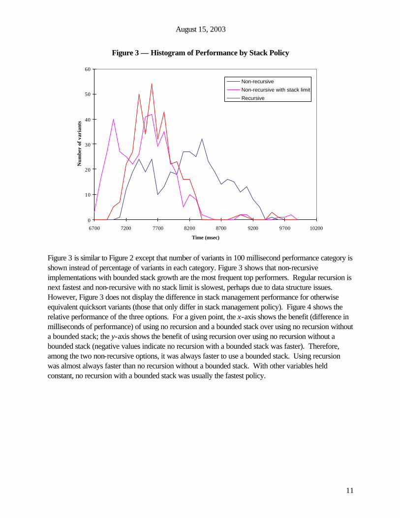
Figure 3 — Histogram of Performance by Stack Policy

0

10

20

30

40

50

60

6700 7200 7700 8200 8700 9200 9700 10200

Time (msec)

Num

ber

of v

aria

nts

Non-recursive

Non-recursive with stack limit

Recursive

Figure 3 is similar to Figure 2 except that number of variants in 100 millisecond performance category is shown instead of percentage of variants in each category. Figure 3 shows that non-recursive implementations with bounded stack growth are the most frequent top performers. Regular recursion is next fastest and non-recursive with no stack limit is slowest, perhaps due to data structure issues. However, Figure 3 does not display the difference in stack management performance for otherwise equivalent quicksort variants (those that only differ in stack management policy). Figure 4 shows the relative performance of the three options. For a given point, the x-axis shows the benefit (difference in milliseconds of performance) of using no recursion and a bounded stack over using no recursion without a bounded stack; the y-axis shows the benefit of using recursion over using no recursion without a bounded stack (negative values indicate no recursion with a bounded stack was faster). Therefore, among the two non-recursive options, it was always faster to use a bounded stack. Using recursion was almost always faster than no recursion without a bounded stack. With other variables held constant, no recursion with a bounded stack was usually the fastest policy.

August 15, 2003

12

Figure 4 — Relative Performance of Different Stack Management Policies

-5000

-4000

-3000

-2000

-1000

0

1000

2000

3000

4000

5000

0 500 1000 1500 2000 2500 3000 3500 4000 4500 5000

Advantage of non-recursive w/stack limit

Adv

anta

ge o

f re

curs

ion

5.2. Insertion Sort: After or During?

Figure 5 — Relative Performance of Insertion Sort During or After Quicksort

0

5

10

15

20

25

30

35

-1000 -800 -600 -400 -200 0 200 400 600 800 1000

TIme Advantage of Insertion Sort During Instead of After

Num

ber

of V

aria

nts

Sedgewick has long suggested performing one insertion sort pass after a quicksort should be faster than interspersed insertion sorts [23] [24]. Bentley & McIlroy found the opposite. At least for the variants

August 15, 2003

13

examined in this project, our results agree with Bentley & McIlroy in most cases. Figure 5 is a histogram of the performance differences between otherwise equivalent quicksort configurations that only differ on whether or not insertion short is interspersed on done afterwards. Results to the right of the y-axis are situations where interspersed insertion sort is faster; this constitutes the majority of the trials. Of the seven fastest quicksort variants generated, only one performed insertion short after the quicksorts. Figure 6 shows that more of the faster quicksorts do insertion sort during the main sorting activity.

Figure 6 — Histogram of Insertion Sort Performance

0

10

20

30

40

50

60

70

6700 7200 7700 8200 8700 9200 9700

Time (milliseconds)

Num

ber

of V

aria

nts

Insertion Sort After

Insetion Sort During

6. Future Work While faster tuning settings were found, much more work remains to be done. For example, the cause of performance shortfalls in the generated variants needs to be explained. By more tailored explorations of the tuning space, greater than 5% improvements might be found. However, benchmark runs also need to be done on different architectures to see how universal and stable the best settings are. Similar searches should be undertaking for other primitive types and more tweaks could be added to the search space. Additionally, the performance of quicksort should also be compared against mergesort, including sophisticated mergesorts which use some of the same tricks as quicksort, such as switching to insertion sort for small arrays [23]. Overall, this study affirms the sound engineering of the Bentley and McIlroy code, although updated tuning settings are probably warranted.

7. Acknowledgments A number of colleagues at Sun helped ease the development of this project. Cliff Click provided insight into the details of HotSpot’s operations. Gilad Bracha fielded questions on tail call elimination in Java. Ken Russell had suggestions on class loaders. Josh Bloch lent his workstation to the bechmarking effort

August 15, 2003

14

and helped guide the threading aspects of the benchmark driver. Finally, Iris Garcia provided programming advice on a number of Java features.

August 15, 2003

15

8. Appendix 1 — Optimization Issues in Java

8.1. Bounds check (range check) elimination A Java program cannot access an array outside of its defined bounds. The most naïve implementation of this requirement checks to make sure each array access is in bounds; e.g. for(int i = 0; i < n; i++) sum +=a[i];

would effectively get run as machine code similar to for(int i = 0; i < n; i++) { if(i >0 and i <= a.length) sum +=a[i]; else throw new ArrayOutOfBoundsException(); }

Since these checks are costly, especially in loops, compilers aim to elide checks on every access by doing a few checks up front that prove the set of array accesses being considered will stay in bounds; this transformation is known as bounds check elimination.

8.2. Tail-call elimination In many languages, when one method calls another, a new stack frame is created to hold the callee’s parameters, local variables, and other information. If that last action a method takes is to call another method, in principle the current stack frame can be reused for the new method (since no information in the caller’s stack frame will ever be re-used). For example in static void factorial(int n, int product) // assume n >= 0 if (n == 0) answer = product; // write final result to external variable else return factorial(n-1, n*product);

the recursive call to factorial could be recognized as a tail-call by the compiler; effectively turning this simple recursion into loop iteration. This transformation is required by the Scheme language so that recursion can be used in place of explicit looping [12].

Java presents a number of challenges to traditional tail-call elimination. Besides altering control flow, in Java a method call can lock an object and establish new exception handlers. Additionally, security in Java can be based on what methods are on the stack and a thrown exception has to be able to rebuild the state of the stack. Because of these considerations, a Java program often needs information about the state of the method call stack. Therefore, analyses much more involved than simple control flow are needed to perform legal tail-call elimination in Java. None of the commonly used JVMs performs tail-call elimination.

August 15, 2003

16

8.3. On tack replacement HotSpot works by gathering profiling information while code is being interpreted and then, if the code is sufficiently “hot,” generates compiled code for that method. The compiled code would be used the next time the method was entered. However, consider the case of a long-running loop inside a method. When the method is first entered, it is interpreted. As the loop runs, profiling information is gathered, and HotSpot generates a compiled version of the method. However, in old versions of HotSpot, since the method is never left or called again, the main loop remains interpreted (although methods the loop calls will be compiled) [18]. Therefore, in such an environment, due to compiler artifacts, any non-recursive version of quicksort would likely run slower than a recursive one since the latter would be compiled while the former would not. Newer version of HotSpot have on stack replacement [11]; that is, a method running in interpreted mode can be replaced by its compiled equivalent while it executes, avoiding this performance anomaly.

9. Appendix 2 — Sample Quicksort Skeleton // Strings between ‘@’ and ‘#’ characters are replaced with appropriate // values. // Asserts were used during development and debuggging but were not enabled // during benchmarking runs. package Sort; public final class QS_pivot@PVN#T@M3T#N@N9T#_part@PPN#_is@ISPN#@IST#_recurY { private final static boolean randomPivot = false; private final static int median3Threshold = @M3T#; private final static int nintherThreshold = @N9T#; private final static int insertSortThreshold = @IST#; private final static boolean insertSortDuring = @ISPV#; private final static boolean partitionClassical = @PPV#; static { assert( ((median3Threshold == 0) || (median3Threshold >= 3)) && ((nintherThreshold == 0) || (nintherThreshold >= 9)) && ((median3Threshold > 0 && nintherThreshold > 0)? (median3Threshold < nintherThreshold):true ) && (insertSortThreshold >= 0) ); } // prevent instantiation private QS_pivot@PVN#T@M3T#N@N9T#_part@PPN#_is@ISPN#@IST#_recurY() {}; public static void sort(int[] a) { if (partitionClassical) quicksort(a, 0, a.length-1); else { quicksort(a, 0, a.length-1, new Pair()); } if(insertSortThreshold != 0 && !insertSortDuring) { QsUtils.insertSort(a, 0, a.length-1);

August 15, 2003

17

} } static void quicksort(int a[], int L, int R) { int p; if(R <= L) return; // code to handle insertion sort options if(insertSortThreshold > 0) { if(insertSortDuring) { if((R-L) <= insertSortThreshold) { QsUtils.insertSort(a, L, R); return; } } else { if((R-L) <= insertSortThreshold) { return; } } } // code to handle partition options if (median3Threshold == 0 && nintherThreshold == 0) { p = QsUtils.partitionCL(a, L, R, QsUtils.findPivot@PVN#(a, L, R)); } else if (median3Threshold > 0) { if(nintherThreshold == 0) { // median of 3 only p = QsUtils.partitionCL(a, L, R, (((R - L) > median3Threshold) ? QsUtils.findPivotM3(a, L, R) : QsUtils.findPivot@PVN#(a, L, R))); } else { // both median and ninther are being used int diff = (R - L); int pivot; assert(diff >= 0); if(diff < median3Threshold) pivot = QsUtils.findPivot@PVN#(a, L, R); else if( diff > nintherThreshold) pivot = QsUtils.findPivotN9(a, L, R); else pivot = QsUtils.findPivotM3(a, L, R); p = QsUtils.partitionCL(a, L, R, pivot); } } else { // nintherThreshold must be non-zero assert(nintherThreshold > 0); p = QsUtils.partitionCL(a, L, R,

August 15, 2003

18

(((R - L) > nintherThreshold) ? QsUtils.findPivotN9(a, L, R) : QsUtils.findPivot@PVN#(a, L, R))); } quicksort(a, L, p-1); quicksort(a, p+1, R); } static void quicksort(int a[], int L, int R, Pair pair) { int p; if(R <= L) return; // code to handle insertion sort options if(insertSortThreshold > 0) { if(insertSortDuring) { if((R-L) <= insertSortThreshold) { QsUtils.insertSort(a, L, R); return; } } else { if((R-L) <= insertSortThreshold) { return; } } } // code to handle partition options if (median3Threshold == 0 && nintherThreshold == 0) { // return new partition regions in pair QsUtils.partitionBM(a, L, R, QsUtils.findPivot@PVN#(a, L, R), pair); } else if (median3Threshold > 0) { if(nintherThreshold == 0) { // median of 3 only QsUtils.partitionBM(a, L, R, (((R - L) > median3Threshold) ? QsUtils.findPivotM3(a, L, R) : QsUtils.findPivot@PVN#(a, L, R)), pair); } else { // both median and ninther are being used int diff = (R - L); int pivot; assert(diff >= 0); if(diff < median3Threshold) pivot = QsUtils.findPivot@PVN#(a, L, R); else if( diff > nintherThreshold) pivot = QsUtils.findPivotN9(a, L, R); else

August 15, 2003

19

pivot = QsUtils.findPivotM3(a, L, R); QsUtils.partitionBM(a, L, R, pivot, pair); } } else { // nintherThreshold must be non-zero assert(nintherThreshold > 0); QsUtils.partitionBM(a, L, R, (((R - L) > nintherThreshold) ? QsUtils.findPivotN9(a, L, R) : QsUtils.findPivot@PVN#(a, L, R)), pair); } quicksort(a, L, pair.L); quicksort(a, pair.R, R); } }

10. References

[1] J. L. Bentley and M. D. McIlroy, “Engineering a sort function,” Software—Practice and Experience, vol. 23, 1993, pp. 1249-1265.

[2] Jeff Bilmes, Krste Asanovic, Chee-whye Chin, Jim Demmel, “Optimizing Matrix Multiply using PHiPAC: a Portable, High-Performance, ANSI C Coding Methodology,” Proceedings of International Conference on Supercomputing, Vienna, Austria, July 1997.

[3] Cliff Click, “High-Performance Computing with the Server Compiler for the Java HotSpot™ Virtual Machine, ” JavaOne Conference, 2001

[4] Cliff Click, “How NOT To Write A Microbenchmark,” JavaOne Conference, 2002.

[5] M. Frigo and S. G. Johnson, “FFTW: An Adaptive Software Architecture for the FFT,” 1998 ICASSP Conference Proceedings, vol. 3, pp. 1381-1384.

[6] James Gosling, Bill Joy, Guy Steele, and Gilda Bracha, The Java™ Language Specification, 2nd edition, Addison-Wesley, 2000.

[7] John L. Hennessy and David A. Patterson. Computer Architecture A Quantitative Approach, Second Edition. Morgan Kaufmann Publishers, Inc., 1996.

[8] J. S. Hillmore, “Certification of Algorithms 63, 64, 65 Partition, Quicksort, Find,” Communications of the ACM vol. 5, no. 8, August 1963, p. 446

[9] C. A. R. Hoare, “Algorithm 63: Partition; Algorithm 64: Quicksort; Algorithm 65: Find,” Communications of the ACM, vol. 4, no. 7, July 1961, pp. 321-322. (See certifications in [8] and [21])

[10] C. A. R. Hoare, “Quicksort,” The Computer Journal, vol. 5, April 1962-January 1963, pp. 10-15.

August 15, 2003

20

[11] Urs Hölzle, Craig Cambers, and David Ungar, “Debugging optimized code with dynamic deoptimization,” Proceedings of the ACM SIGPLAN '92 Conference on Programming Language Design and Implementation, June 1992, pp. 32-43.

[12] Richard Kelsey, William Clinger, And Jonathan Rees (Editors), “Revised5 Report on the Algorithmic Language Scheme,” In Higher-Order and Symbolic Computation (formerly: LISP and Symbolic Computation) Volume 11, Issue 1, August, 1998.

[13] Donald E. Knuth, The Art of Computer Programming Volume 1/Fundamental Algorithms, Second Edition, Addison Wesley, 1973.

[14] Donald E. Knuth, The Art of Computer Programming Volume 3/Sorting and Searching, Second Edition, Addison Wesley, 1998

[15] Sheng Liang and Gilad Bracha, “Dynamic Class Loading in the Java™ Virtual Machine,” Proceedings of the 13th Annual ACM SIGPLAN Conference on Object-Oriented Programming Systems, Languages, and Applications (OOPSLA ’98), 1998.

[16] Tim Lindholm and Frank Yellin, The Java™ Virtual Machine Specification, Second Edition, Addison-Wesley, 1999.

[17] M. D. McIlroy, “A Killer Adversary for Quicksort,” Software—Practice and Experience, vol. 29, 1999, pp. 1-4.

[18] Steve Meloan, “The Java HotSpot™ Performance Engine: An In-Depth Look,” Java Developer Connection, June 1999, http://developer.java.sun.com/developer/technicalArticles/Networking/HotSpot/.

[19] José Moura, Jeremy Johnson, Robert W. Johnson, David Padua, Viktor Prasanna, Markus Püschel, and Manuela Veloso, “SPIRAL: Automatic Implementation of Signal Processing Algorithms,” Proceedings High Performance Embedded Computing (HPEC) 2000, MIT Lincoln Laboratories.

[20] Michael Paleczny, Christopher Vick, and Cliff Click, “The Java HotSpot™ Server Compiler,” Java™ Virtual Machine Research and Technology Symposium April 23–24, 2001, Monterey, California.

[21] B. Randell and L. J. Russell, “Certification of Algorithms 63, 64, and 65, Partition, Quicksort, and Find,” Communications of the ACM, vol. 6, no. 8, August 1963, pp 446.

[22] Michel Schinz and Martin Odersky, “Tail call elimination on the Java Virtual Machine,” Proceedings ACM SIGPLAN BABEL'01 Workshop on Multi-Language Infrastructure and Interoperability, 2001, pp. 155-168.[23] Robert Sedgewick, Algorithms in C, Third Edition, Addison-Wesley, 1998.

[24] Robert Sedgewick, “The Analysis of Quicksort Programs,” Acta Informatica, vol. 7, 1976/77, pp. 327-356.

[25] Robert Sedgewick, “Implementing Quicksort Programs,” Communications of the ACM, vol. 21, no. 10, 1978, pp. 847-857.

August 15, 2003

21

[26] Robert Sedgewick, Quicksort, Ph.D. Thesis, Stanford University, Stanford Computer Science Report STAN-CS-75-492, May 1975.

[27] Robert Sedgewick, “Quicksort with Equal Keys,” Siam Journal on Computing, vol. 6, no. 2, June 1977, pp. 240-267.

[28] R. C. Singleton, “An efficient algorithm for sorting with minimal storage (Algorithm 347),” Communications of the ACM, vol 12, 1969, pp. 185-187.

[29] Richard Vuduc, James W. Demmel, and Jeff Bilmes, Statistical modeling of feedback data in an automatic tuning system, In MIRCO-33: Third ACM Workshop on Feedback-Directed Dynamic Optimization, December 2000.

[30] D. W. Wall, “Register Windows vs. Register Allocation,” Proceedings of the SIGPLAN '88 Conference on Programming Language Design and Implementation, June 1988

[31] David L. Weaver and Tom Germond, ed., The SPARC Architecture Manual, version 9, Prentice Hall, 1994.

[32] R. Clint Whaley, Antoine Petite, and Jack J. Dongarra, “Automated Empirical Optimization of Software and the ATLAS Project,” LAPACK Working Note 147, September 19, 2000, http://www.netlib.org/lapack/lawns/lawn147.ps.