finding the best k in core decomposition: a time and space
TRANSCRIPT

Finding the Best k in Core Decomposition:A Time and Space Optimal Solution
Deming Chu?†, Fan Zhang?, Xuemin Lin§, Wenjie Zhang§, Ying Zhang], Yinglong Xia‡, Chenyi Zhang\
?Guangzhou University, †East China Normal University, §University of New South Wales]University of Technology Sydney, ‡Facebook AI, \Huawei Technologies
{ned.deming.chu, fanzhang.cs}@gmail.com, {lxue, zhangw}@[email protected], [email protected], [email protected]
Abstract—The mode of k-core and its hierarchical decompo-sition have been applied in many areas, such as sociology, theworld wide web, and biology. Algorithms on related studies oftenneed an input value of parameter k, while there is no existingsolution other than manual selection. In this paper, given a graphand a scoring metric, we aim to efficiently find the best valueof k such that the score of the k-core (or k-core set) is thehighest. The problem is challenging because there are variouscommunity scoring metrics and the computation is costly on largedatasets. With the well-designed vertex ordering techniques, wepropose time and space optimal algorithms to compute the best k,which are applicable to most community metrics. The proposedalgorithms can compute the score of every k-core (set) and canbenefit the solutions to other k-core related problems. Extensiveexperiments are conducted on 10 real-world networks with sizeup to billion-scale, which validates both the efficiency of ouralgorithms and the effectiveness of the resulting k-cores.
I. INTRODUCTION
Graphs are widely adopted to model the structure of com-plex networks with a large spectrum of applications. As afundamental graph problem, cohesive subgraph mining is toextract groups of densely connected vertices. The well-studiedmodel of k-core is defined as a maximal connected subgraph inwhich every vertex is connected to at least k other vertices inthe same subgraph [42], [51]. We use k-core set to denote thesubgraph formed by all the (connected) k-cores in the graph,for a fixed parameter k. The hierarchical decomposition byk-core (or core decomposition) computes the k-core set forevery possible k. The hierarchy of core decomposition buildson the containment property of k-core sets: the (k + 1)-coreset is always a subgraph of the k-core set.
The k-core and its hierarchical structure have a wide rangeof applications, such as finding communities in the web [22]and social networks [25], [57], [65], discovering molecularcomplexes in protein interaction networks [6], recognizinghub-nodes in brain functional networks [8], analyzing un-derlying structure of the Internet and its functional conse-quences [10], understanding software systems using softwarenetworks [66], and predicting structural collapse in mutualisticecosystems [44].
Despite the elegant structure of k-core hierarchy and thevarious applications, a common open problem is to find the
∗Deming Chu and Fan Zhang are the joint first authors. Fan Zhang is thecorresponding author.
best k-core set or the best single k-core. To the best of ourknowledge, there is no previous work that studies the best kvalue for k-core and for other models of cohesive subgraph,e.g. k-truss, k-plex, k-vcc, k-ecc. The existing solution isto simply adopt the user-defined k, or to determine k bytrivial statistics, e.g., setting k to average vertex degree. Theunderlying problem is essentially to ask the quality of the k-cores, since different input values lead to different k-cores. Inthis paper, given a graph and a community scoring metric, weaim to efficiently compute a value of k such that the k-coreset has the highest score among all the k-core sets for everyinteger k. Besides, we also aim to efficiently find a best singlek-core among all the k-cores for every integer k.
There is no uniform metric to evaluate the quality of asubgraph [63]. Different community scoring metrics are de-signed for different objectives considering particular networkproperties [11], [63]. For example, clustering coefficient is agoodness metric for clustering tendency [59], and modularitymeasures the quality of a graph partition [45], [46]. To applyour proposed algorithms to various community metrics andeven new metrics, we extract representative primary valueswhich can be utilized to calculate most community scores [11].
A basic solution of finding the best k is to conduct qualitycomputation on the k-core set for every possible input of k.In our preliminary experiments, for a graph that can be loadedinto memory within 100 seconds, the basic solution spentmore than one day for some scoring metrics. To efficientlyhandle billion-scale graphs, we design a light-weight vertexordering procedure to facilitate incremental score computation.We compute the score of k-core sets from the center core ofthe graph to the margins, with optimal time and space cost.
Our paradigm can also be applied to find a best single k-core when the connectivity of different k-cores is consideredin the computation. The score of every k-core (set) can beretrieved by our algorithms. Moreover, our algorithm canhelp solve other k-core related problems, e.g., finding densestsubgraph, maximum clique, and size-constrained k-core. Theexperiments in the paper show that our algorithm can serve asbetter approximate solutions compared to the state-of-the-artor produce useful intermediate results.
Example 1. Figure 1 illustrates the hierarchy of a networkdecomposed by the k-core model, where k varies from 1 to3. When k = 1, the 1-core (set) is whole graph, i.e., G1.

𝑘 = 3
𝑘 = 2
𝐺3.1 𝐺3.2
𝑘 = 1
𝐺2
𝐺1Fig. 1. Hierarchical Core Decomposition
When k = 2, the k-core decomposition recursively deletesevery vertex with degree less than 2, resulting in the 2-core(set) G2. When k = 3, the 3-core set consists of two 3-cores:G3.1 and G3.2.
Suppose the scoring metric is average degree (twice thenumber of edges divided by the number of vertices), (i) thebest k-core set is the 3-core set, because it has the highestscore (average degree) among all the k-core sets, and thebest k is 3; and (ii) the best single k-core is G3,1 as it hasthe highest score among all the k-cores with different k.
Contributions. The principal contributions in this paper aresummarized as follows.• To the best of our knowledge, this is the first work to
study the following problems: given a graph G and acommunity scoring metric Q, (i) find the best k-core set;and (ii) find a best single k-core, according to Q.
• We develop efficient and extensible algorithms to solveour proposed problems. We prove the algorithms areworst-case optimal in both time and space complexities.For many scoring metrics, our score computation can re-turn in O(n) time where n is the number of vertices in thegraph. The algorithms can apply to various communitymetrics and can shed light on finding the best k for otherdecomposition models.
• Extensive experiments are conducted on 10 real graphswith up to billions of edges. The results show that thequality of k-core (set) with the resulting k is much betterthan that with user-defined k or other trivial values. To-wards efficiency, our algorithms outperform the baselinesby 1-4 orders of magnitude in runtime. For some k-core related problems, our algorithms can serve as goodapproximate solutions or benefit the algorithm design.
II. PRELIMINARIES
We consider an undirected and unweighted simple graphG = (V,E), with n = |V | vertices and m = |E| edges(assume m > n). Given a vertex v in a subgraph S, N(v, S)denotes the neighbor set of v in S, i.e., N(v, S) = {u |(u, v) ∈ E(S)}. The degree of v in subgraph S, i.e., |N(v, S)|,is denoted by d(v, S). For the input graph G, we omit G inthe notations when the context is clear, e.g., we abbreviateN(v,G) to N(v). Table I summarizes the notations.
A. Core Decomposition
The model of k-core [42], [51] is defined as follows.
TABLE ISUMMARY OF NOTATIONS
Notation DefinitionG = (V,E) an undirected, unweighted simple graphn;m number of vertices/edges in G (m > n)S a subgraph of GV (S) the set of vertices in SE(S) the set of edges in Sid(v) unique identification of v in GN(v);N(v, S) the set of neighbors of v in G / in Sd(v); d(v, S) degree of v in G / in SCk the k-core set of Gc(v) coreness of v in G, max{k | v ∈ Ck}kmax largest k s.t. Ck is not emptyHk the k-shell of G, {v | c(v) = k}rank(v) the ranking of vertex v in Vn(S) number of vertices in Sm(S) number of edges in Sb(S) number of boundary edges of S∆(S) number of triangles in St(S) number of triplets in S
Definition 1 (k-Core). Given a graph G and an integer k, asubgraph S is a k-core of G, if (i) each vertex v ∈ S has atleast k neighbors in S, i.e., d(v, S) ≥ k; (ii) S is connected;and (iii) S is maximal, i.e., any supergraph of S is not a k-coreexcept S itself.
We use the k-core set to denote the subgraph containingevery (connected) k-core with a fixed parameter k.
Definition 2 (k-Core Set). Given a graph G and an integerk, the k-core set of G, denoted by Ck, is the subgraph formedby all the (connected) k-cores in G.
If an integer k′ ≥ k, the k′-core set is always a subgraph ofthe k-core set, i.e., Ck′ ⊆ Ck. This implies that each vertexin a graph has a unique number of coreness [7].
Definition 3 (Coreness and k-Shell). Given a graph G, thecoreness of a vertex v ∈ G is c(v) = max{k | v ∈ Ck},i.e., the largest k such that the vertex v is in the k-core. Thek-shell of G is Hk = {v | c(v) = k}, i.e., the set of verticeswith coreness k.
We use kmax (graph degeneracy) to denote the largestcoreness in G, i.e., the largest k such that the k-core of Gis not empty.
Definition 4 (Core Decomposition). Given a graph G, coredecomposition is to compute the coreness c(v) for every vertexv ∈ V (G).
The algorithm for core decomposition is to recursivelyremove the vertex with the smallest degree in the graph, withtime complexity of O(m) [7].
Example 2. Figure 2 shows a graph of 12 vertices. Thegraph itself is a 2-core. When k = 3, the k-core computationrecursively deletes every vertex with degree less than 3, i.e.,v5, v7, v6 and v8. The 3-core set is the induced subgraph bythe rest vertices. The coreness of v5, v7, v6 and v8 is 2, and

𝑣4
𝑣1 𝑣3
𝑣2
𝑣12
𝑣9 𝑣11
𝑣10
𝑣8𝑣6
𝑣5
𝑣7
Fig. 2. A 2-core graph in which the 3-core is circled
the coreness of other vertices is 3. There are two connectedcomponents (3-cores) in the 3-core set, as circled in the figure.
B. Problem DefinitionWe are the first to propose and study the following problems
of finding the best k-core (set).• find the k∗-core set Ck∗ such that it has the highest score
among all the k-core sets for every integer k with 0 ≤k ≤ kmax;
• find the k∗-core S such that it has the highest scoreamong all the k-cores for every integer k with 0 ≤ k ≤kmax.
C. Community Scoring MetricsAlthough there are various community scoring metrics
considering different community properties, most of them areconstructed on the following primary values [63].Primary Values. Let S be a subgraph to evaluate, we studythe following common primary values.• n(S): the number of vertices in S, i.e., n(S) = |V (S)|;• m(S): the number of edges in S, i.e., m(S) = |E(S)|;• b(S): the number of boundary edges in S, b(S) =|{(u, v) | (u, v) ∈ E, u ∈ S, v 6∈ S}|;
• ∆(S), the number of triangles in S;• t(S), the number of triplets (three vertices connected by
two edges) in S, i.e., t(S) =∑v∈S
(d(v,S)
2
);
Metrics. Based on the above primary values, some communityscoring metrics are defined as follows.• Average Degree: f(S) = 2×m(S)
n(S) is the average degreeof vertices in S;
• Internal Density: f(S) = 2×m(S)n(S)×(n(S)−1) is the internal
density of vertices in S;• Cut Ratio: f(S) = 1 − b(S)
n(S)×(n−n(S)) is the differenceof 1 and the fraction of existing boundary edges over allthe possible ones;
• Conductance: f(S) = 1− b(S)2×m(S)+b(S) is the difference
of 1 and the proportion of degrees where the vertex pointsto the outside;
• Modularity: f(P ) =k∑i=1
(m(Pi)m −
(2×m(Pi)+b(Pi)
2×m
)2)
is the modularity for a partition P on G, where Pi is theith community in the partition [46];
• Clustering Coefficient: f(S) = 3×∆(S)t(S) measures the
tendency of vertices to cluster together;Given a scoring metric, for an integer k, the target subgraphs
for computing the scores are all the k-cores with the given k,i.e., the subgraphs in Ck.
III. FINDING THE BEST K-CORE SET
In this section, we propose the solution to find the best kfor the k-core set, including the baseline in Section III-A, andthe improved algorithm in the rest sections.
A. Baseline Algorithm
Given a graph G and a community scoring metric Q, abaseline solution is to first conduct core decomposition, orderthe vertices by coreness to fast retrieve a k-core set, and thencompute the score of every k-core set according to Q, forevery integer k with 0 ≤ k ≤ kmax.
We use a bin sort to order the vertices in G by coreness,and record every start position of the vertices with the samecoreness, which takes O(n) time. Then, retrieving the vertexset of a k-core set Ck takes O(|V (Ck)|) time. Let O(qk)be the time cost to compute the score of Ck given V (Ck),Q and G. The time complexity of the baseline algorithm isO(∑kmax
k=0 (qk + |V (Ck)|))
. Although the baseline runs inpolynomial time, it is costly to handle large graphs.
B. Vertex Ordering for Optimal Neighbor Query
In order to compute the best k in optimal time and spacecost, we first introduce the vertex ordering techniques.
We divide the vertices in G into kmax + 1 arrays whereeach is associated with a unique coreness value. The arrays areordered by the associated coreness to fast locate the verticeswith different coreness.
For every vertex v in G, the neighbor set of v is ordered byincreasing values of vertex rank which is defined as follows.
Definition 5 (Vertex Rank). Given two vertices u and v, therank of v is higher than u, denoted by rank(v) > rank(u),if (i) c(v) > c(u); OR (ii) c(v) = c(u) and id(v) > id(u),where id(v) is the unique identification of v.
For every vertex v, to efficiently retrieve specific parts ofits neighbour set, we also record some position tags wheresame is the position of the first u in N(v) such that c(u) ≥c(v), plus is the position of the first u in N(v) such thatc(u) > c(v), and high is the position of the first u in N(v)such that rank(u) > rank(v). The above tag is set to |N(v)|when there is no such u ∈ N(v) satisfying the condition. Theordering is summarized in Table II.
Algorithm 1 shows the pseudo-code for vertex ordering.At Line 1-4, we use kmax + 1 bins to sort vertices by rank,where each bin represents a unique value of coreness. Inspiredby [33], we flatten kmax + 1 bins to sort the edge set: (i) AtLine 5-8, for every vertex v with ascending order of vertex id,we push the pair (v, u) from every neighbor u of v into thebin represented by the coreness of v; (ii) At Line 9-11, weretrieve the sorting from the kmax + 1 bins by one scan frombin 0 to bin kmax, where N ′(u) is empty initially for everyu ∈ V . For every element (v, u) in the bins, we push v intothe new neighbor set of u s.t. the neighbors of u are orderedby vertex rank. Besides, we record the subscripts in Table IIfor each vertex via one scan of the new edge set (Line 13).Complexity of Vertex Ordering and Query. In Algorithm 1,the sorting of vertices takes O(n) since every vertex is visited

TABLE IITHE ORDERED NEIGHBOR SET OF v
Subscript of u ∈ N(v) Constraint of u Vertex Set[0, same− 1] c(u) < c(v) N(v,<)[same, plus− 1] c(u) = c(v) N(v,=)[plus, |N(v)| − 1] c(u) > c(v) N(v,>)[same, |N(v)| − 1] c(u) ≥ c(v) N(v,≥)[high, |N(v)| − 1] rank(u) > rank(v) N(v,>r)
Every u in N(v) is ordered by ascending order of rank;same: position of the first u ∈ N(v) s.t. c(u) ≥ c(v);plus: position of the first u ∈ N(v) s.t. c(u) > c(v);
high: position of the first u ∈ N(v) s.t. rank(u) > rank(v).
Algorithm 1: vertex orderingInput : a graph G = (V,E), the coreness c(v) of every
vertex v ∈ VOutput : G with ordered V and E by vertex rank, and
position tags/* Order vertex set V */bin1← a list of (kmax + 1) empty arrays;1for each v in V with ascending order of vertex id do2
bin1[c(v)].push_back(v);3
V ← concatenation of bin1[0],bin1[1], ...,bin1[kmax];4/* Order edge set E */bin2← a list of (kmax + 1) empty arrays;5for each v in V with ascending order of vertex id do6
for each u in N(v) do7bin2[c(v)].push_back(pair(v, u));8
for each i from 0 to kmax do9for each element (v, u) in bin2[i] from head to tail do10
N ′(u).push_back(v);11
E ← each v ∈ V has neighbors N ′(v);12same, plus and high of v ← scan N ′(v) for every v ∈ V ;13return G = (V,E) with ordered V and E, and position tags14
twice, and the sorting of the edge set takes O(m) since everyedge is visited at most 5 times. The overall time complexityis O(m). The space complexity is dominated by the size ofthe graph which is O(m).
After the vertex ordering, according to Table II, we cananswer |N(v, ·)| in O(1) time, e.g., |N(v,=)| = plus−same,and return N(v, ·) in O(|N(v, ·)|) time.
Example 3. Figure 3 illustrates the vertex ordering for thegraph in Figure 2. Each vertex in Figure 3 is colored accordingto different coreness values. On the top, all the vertices areordered by coreness with ties broken by vertex id. The verticesin every neighbor set are also sorted by the above order. Inthe figure, we show the ordered neighbor sets of four verticesand their position tags. For vertex v1 and v9, the position plusequals to the length of the neighbor set because the corenessof any neighbor is not larger than the vertex. By checking theordering results and Table II, all types of |N(v, ·)| queries canbe answered in O(1), e.g., |N(v6, >)| = |N(v6)| − plus = 1.
C. The Improved Algorithm
An important property of hierarchical core decompositionis its containment nature: Ck+1 ⊆ Ck for every coreness k.This suggests that the primary values of the k-core set can be
Vertex Ordered Neighbors 𝑠𝑎𝑚𝑒 𝑝𝑙𝑢𝑠 ℎ𝑖𝑔ℎ
0 3 0
0 3 1
0 2 2
1 4 1
𝑣1
𝑐 𝑣 = 2 𝑐 𝑣 = 3
𝑣2 𝑣3
𝑣6 𝑣3𝑣5 𝑣7 𝑣8
𝑣8 𝑣9𝑣6 𝑣7
𝑣9 𝑣11𝑣8 𝑣10
𝑣8𝑣5 𝑣6 𝑣7 𝑣12𝑣9 𝑣10 𝑣11𝑣4𝑣1 𝑣2 𝑣3
𝑣4
𝑣12
Fig. 3. Example of Vertex Ordering
Algorithm 2: computing the best kInput : a graph G, a community scoring metric QOutput : the best k value for a k-core setcompute each k-core set Ck by core decomposition;1order G by Algorithm 1;2metric← [0, . . . , 0];3in← 0,out← 0,num← 0;4for each integer k from kmax to 0 do5
for v ∈ Hk do6in← in+ |N(v,>)|+ 1
2|N(v,=)|;7
out← out+ |N(v,<)| − |N(v,>)|;8num← num+ 1;9
metric[k]← compute_metric(Q,in,out,num);10
return metric11
incrementally derived from the primary values of the (k+ 1)-core set, with minor modification according to their difference.Based on the above observation, we compute the scores of thek-core sets in a top-down manner, i.e., for k from kmax to0. Note that it is costly to count some primary values in abottom-up manner, i.e., for k from 0 to kmax.
Algorithm 2 shows the pseudo-code for computing thebest k. The algorithm incrementally computes and updatesthe primary values of k-core sets. Note that we present thecomputation for clustering coefficient in Section III-D. InAlgorithm 2, array metric records the score of every k-coreset. Let S be the subgraph induced by the visited vertices atLine 6. Variable in records the number of internal edges ofS. Variable out records the number of boundary edges of Swhere each edge has exactly one endpoint in S. Variable numrecords the number of visited vertices.
Line 3-4 initializes array metric and the primary values.Line 5-10 incrementally compute the score of the k-core setfrom k = kmax to k = 0. For each value of k, we only visitthe vertices with coreness k at Line 6, and update the primaryvalues at Line 7-9. Based on the primary values for the (k+1)-core set, we update the values by considering every neighboru of the visited vertex v as follows.
• If c(u) = c(v), then (u, v) should be counted in the valuein. Because (u, v) will be counted in in when we visitboth u and v at Line 6, we add 1
2 |N(v,=)| to in forvisiting v.
• If c(u) < c(v), then (u, v) should be counted in the valueout. Because (u, v) will only be counted in out when v

is visited at Line 6, we add |N(v,<)| to out for visitingv.
• If c(u) > c(v), then u ∈ Ck+1 and (u, v) /∈ Ck+1, i.e.,(u, v) is a boundary edge of the (k+ 1)-core set. For thek-core, (u, v) becomes an internal edge since (u, v) ∈Ck(G). So we add |N(v,>)| to in and subtract |N(v,>)| from out.
In Line 10, the community score is calculated from theprimary values, e.g., the average degree of a k-core set is2 × in/num, the cut ratio is 1 − out/(num × (n − num)),etc. Line 11 returns the result.
Example 4. Given a community scoring metric such asaverage degree, the execution of Algorithm 2 on the graph inFigure 2 is as follows. First, we compute the primary valuesof the 3-core set by visiting every vertex v in the 3-core set.Because there are 8 vertices in C3, and every v ∈ C3 has|N(v,>)| = 0 and |N(v,=)| = 3, the number of internaledges in the 3-core set is in = 8×(0+3/2) = 12. The averagedegree of 3-core set is 2×12/8 = 3. Then we visit each vertexin 2-shell and incrementally count the internal edges in 2-core. When v5, v6, v7 and v8 are sequentially visited, we havein = 12+(1+1/2)+(1+3/2)+(0+2/2)+(1+2/2) = 19.The average degree of 2-core set is 2× 19/12 ≈ 3.17. So 2-core set is preferred when the metric is average degree.
Correctness. The correctness of Algorithm 2 is based on thecorrect computation of primary values for every k-core set,which is immediate according to the definitions of primaryvalues, the containment property of k-cores, and Line 7-9.Complexity. (Space) The space complexity is dominated bythe size of the graph which takes O(m). (Time) Benefittingfrom the ordering in Section III-B, |N(v, ·)| can be retrieved inO(1) time for every vertex v. The calculation of a communityscore takes O(1). Each vertex is visited exactly once inAlgorithm 2. The score computation in Algorithm 2 takesO(n). Both core decomposition and vertex ordering takeO(m). The time complexity of Algorithm 2 is O(m).Optimality. Since the time or space complexity of computingan existing community metric on G is at least O(m) [11], theworst-case complexity of Algorithm 2 is optimal.
D. Computation of Triangles and Triplets
Algorithm 3 shows the variant of Algorithm 2 for computingthe best k when the community metric is based on trianglesand triplets, e.g., clustering coefficient. Similar to Algorithm 2,we incrementally compute the primary values in a top-downmanner: from k = kmax to k = 0. For every k-core set,array metric records its score, variable triangle recordsthe number of triangles, and variable triplet records thenumber of triplets. They are initialized in Line 1-2.Triangle Counting. At Line 7-12, the algorithm incrementallyupdates the number of triangles in the k-core set based on thatin the (k+ 1)-core set. For each edge (u, v) with rank(u) >rank(v) (Line 7-8), we count the triangles containing (u, v)by visiting the neighbors of x where x is the one in {u, v} withsmaller degree (Line 9-12). To count triangles, we enumerate
Algorithm 3: computing k by triangles and tripletsInput : a graph G, a community scoring metric QOutput : the best k value for a k-core setmetric← [0, . . . , 0];1triangle← 0,triplet← 0;2f>[v]← f≥[v]← 0 for each v ∈ V ;3compute each k-core set Ck by core decomposition;4order G by Algorithm 1;5for each k from kmax to 0 do6
for v ∈ Hk do7for u ∈ N(v,>r) do8
x← u, y ← v;9swap(x, y) if deg(x) > deg(y) ;10for w ∈ N(x,>r) do11
triangle← triangle+ 1 if12w ∈ N(y,>r);
triplet← triplet+(|N(v,≥)|
2
);13
kshell_nbr←⋃
u∈HkN(u,>);14
for v ∈ kshell_nbr do15f>[v]← f≥[v];16
for v ∈ Hk do17for u ∈ N(v) do18
f≥[u]← f≥[u] + 1;19
for v ∈ kshell_nbr do20gt k ← f>[v], eq k ← f≥[v]− f>[v];21triplet← triplet+
(eq k2
)+ gt k × eq k;22
metric[k]←23compute_metric(Q,triangle,triplet);
return metric24
each vertex w in N(x,>r) and check if w is also in N(y,>r).By visiting N(·, >r) of each vertex, we ensure rank(w) >rank(u) > rank(v) for every counted triangle, i.e., everytriangle is counted for exactly once since we count the threevertices by increasing order of vertex rank.
Triplet Counting. Recall that a triplet 〈u, v, w〉 is formedby three vertices connected by two edges (v, u) and (v, w),centered on v. (i) For each center vertex v in Hk, any pair ofthe neighbors of v in the k-core can form a triplet centered onv. Line 13 adds the number of such pairs to triplet. (ii)Line 14-22 counts the new triplets centered on the vertices ofthe (k + 1)-core set.
We use f>[v] and f≥[v] to count the number of u ∈ N(v)such that c(u) > k and c(u) ≥ k, respectively. Here we do notuse N(v, ·), because a neighbor query in Section III-B onlyworks for vertices in the k-shell, i.e., f>[v] = |N(v,>)| andf≥[v] = |N(v,≥)| iff k = c(v). Line 14 collects the verticesin N(u,>) of every u with coreness k, because they are thecenter vertices in the (k + 1)-core set. Line 15-19 computesf>[v] and f≥[v] for every vertex v in the (k+ 1)-core set, byupdating the values from the previous iteration.
Line 20 iterates over each center vertex in the (k+ 1)-coreset, and Line 21 assigns to gt k and eq k the number of v’sneighbor u such that c(u) > k and c(u) = k, respectively. Toform a triplet (uncounted) with a center vertex in the (k+ 1)-core set, (a) the other two vertices are from Hk; or (b) onevertex is from Ck+1 and the other is from Hk. In Line 22,
(eq k
2
)is the number of the triplets in case (a), and gt k×eq k
is the number of the triplets in case (b).The community score is calculated in Line 23 using the
primary values, e.g., the clustering coefficient of a k-core is3× triangle/triplet. Line 24 returns the result.
Example 5. Given a community scoring metric such asclustering coefficient, the execution of Algorithm 3 on thegraph in Figure 2 is as follows. We first compute the numberof triangles and triplets in 3-core set by Line 7-13: triangle = 8 and triplet = 24. The clustering coefficientof 3-core is 3 × 8/24 = 1. Then, we incrementally computethe values for 2-core set. Line 7-12 detect two new triangles(v5, v6, v3) and (v6, v7, v8), so triangle = 8 + 2 = 10.Line 13 detects
(22
)new triplets for v5,
(42
)for v6,
(22
)for v7,
and(
32
)for v8. Line 22 iterates over kshell_nbr, that is
{v3, v9}, and counts(
22
)+ 3× 2 new triplets for v3 and 3× 1
new triplets for v9. To sum up, triplet = 24+21 = 45. Theclustering coefficient of 2-core is 3 × 10/45 ≈ 0.67. So, the3-core set is preferred when the metric is clustering coefficient.
Correctness. For every triangle (v, u, w) in a k-core but notin a (k+1)-core, suppose rank(v) < rank(u) < rank(w), vis certainly in k-shell; otherwise, (v, u, w) is in a (k+1)-coreaccording to vertex rank, a contradiction. Every such triangleis counted exactly once in Line 7-12, since the visiting of v,u, and w is unique according to their increasing vertex rank.
For every triplet 〈u, v, w〉 in a k-core but not in a (k +1)-core, when the center vertex v is in the k-shell, Line 13correctly counts such triplets. When k = kmax, f≥[v] of everyv ∈ Ckmax
is correctly generated by Line 17-19. For the nextiteration k = kmax−1, f>[v] of every v ∈ Ckmax
is correctlyassigned by f≥[v] from last iteration (Line 15-16). Then f≥[u]of every u ∈ Ckmax−1 is correctly updated by visiting theneighbors of every v ∈ Hk. For every k, f≥[v] and f>[v]for every v ∈ Ck+1 are correct by induction. For every v ∈kshell_nbr, the correctness of gt k, eq k and tripletimmediately follows. The community score is correct basedon the correct primary values.
Complexity. (Space) The space complexity is dominated bythe size of graph which takes O(m). (Time.A) The time costfor triangle counting is O(m1.5). We prove N(z,>r) ≤ 2
√m,
for every vertex z visited in Line 7-12. If deg(z) ≤√m,
then |N(z,>r)| ≤ deg(z) ≤ 2√m. If deg(z) >
√m, we
prove by contradiction. Suppose |N(z,>r)| > 2√m, for
every vertex v ∈ N(z,>r), |N(v,>r)| ≥ |N(z,>r)| >2√m since the vertex rank obeys degeneracy ordering. Then∑v∈N(z,>r) deg(v) ≥ deg(z) · |N(z,>r)| >
√m · 2
√m =
2m, contradict with∑v∈N(z,>r) deg(v) ≤ 2m. So the time
cost is∑v∈V (|N(v,>r)|·deg(v)) ≤
∑v∈V (2
√m·deg(v)) =
2√m ·m = O(m1.5). (Time.B) For triplet counting, Line 13
costs O(n) time, as each vertex is visited once. Maintainingf>[·] and f≥[·] costs O(m), because each edge is visited atmost three times (Line 14 and 18). So triplet counting costsO(m) time. The time complexity of Algorithm 3 is O(m1.5).
Optimality. The time complexity and space complexity oftriangle counting are O(m1.5) and O(m), respectively [35].
3-core
2-core
𝑁𝑆2 𝑁𝑆3
𝑣4
𝑣1 𝑣3
𝑣2
𝑣12
𝑣9 𝑣11
𝑣10
𝑣8𝑣6
𝑣5
𝑣7
𝑣4
𝑣1 𝑣3
𝑣2
𝑣12
𝑣9 𝑣11
𝑣10
𝑁𝑆1
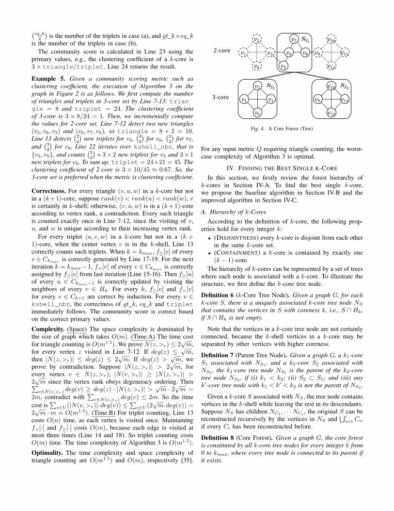
Fig. 4. A Core Forest (Tree)
For any input metric Q requiring triangle counting, the worst-case complexity of Algorithm 3 is optimal.
IV. FINDING THE BEST SINGLE K-CORE
In this section, we firstly review the forest hierarchy ofk-cores in Section IV-A. To find the best single k-core,we propose the baseline algorithm in Section IV-B and theimproved algorithm in Section IV-C.
A. Hierarchy of k-CoresAccording to the definition of k-core, the following prop-
erties hold for every integer k:• (DISJOINTNESS) every k-core is disjoint from each other
in the same k-core set.• (CONTAINMENT) a k-core is contained by exactly one
(k − 1)-core.The hierarchy of k-cores can be represented by a set of trees
where each node is associated with a k-core. To illustrate thestructure, we first define the k-core tree node.
Definition 6 (k-Core Tree Node). Given a graph G, for eachk-core S, there is a uniquely associated k-core tree node NSthat contains the vertices in S with coreness k, i.e., S ∩Hk,if S ∩Hk is not empty.
Note that the vertices in a k-core tree node are not certainlyconnected, because the k-shell vertices in a k-core may beseparated by other vertices with higher coreness.
Definition 7 (Parent Tree Node). Given a graph G, a k1-coreS1 associated with NS1
, and a k2-core S2 associated withNS2
, the k1-core tree node NS1is the parent of the k2-core
tree node NS2, if (i) k1 < k2; (ii) S2 ⊂ S1; and (iii) any
k′-core tree node with k1 < k′ < k2 is not the parent of NS2.
Given a k-core S associated with NS , the tree node containsvertices in the k-shell while leaving the rest in its descendants.Suppose NS has children NC1
, · · ·NCc, the original S can be
reconstructed recursively by the vertices in NS and⋃ci=1 Ci,
if every Ci has been reconstructed before.
Definition 8 (Core Forest). Given a graph G, the core forestis constituted by all k-core tree nodes for every integer k from0 to kmax, where every tree node is connected to its parent ifit exists.

Algorithm 4: the LCPS algorithmInput : a graph G = (V,E), the coreness c(v) of every
vertex v ∈ VOutput : a forest of k-cores of GX ← ∅;1bin← a list of (kmax + 1) empty arrays;2for any u ∈ V \X do3
cur p← the root of a new tree, k ← 0;4bin[0]← bin[0] ∪ {u};5while there exists non-empty array in bin do6
r ← the largest r such that bin[r] is non-empty;7pop v from bin[r];8if v 6∈ X then9
if k > r then adjust cur p so that k ← r;10if c(v) > r then adjust cur p so that k ← c(v);11insert v into the tree node pointed by cur p;12X ← X ∪ {v};13for each w ∈ N(v) \X do14
p← min{c(w), c(v)};15bin[p]← bin[p] ∪ {w};16
return the forest17
The above forest organizes all k-cores into a hierarchy,where each tree corresponds to a connected component of theoriginal graph. The core forest can be stored in O(n) space,because each vertex exists in exactly one tree node and eachtree node has exactly one parent.
Example 6. Figure 4 shows the core forest of Figure 2 whichhas only one tree. There are three tree nodes NS1 , NS2 , andNS3
, associated with S1, S2, and S3, respectively. NS1is
associated with the whole graph (a 2-core) while only thevertices in the 2-shell are contained in NS1
. Although NS1is
also a 1-core, no 1-core tree node would be built accordingto our definition. We can reconstruct S1 from the vertices inNS1
, S2, and S3. Also, we have |S1| = |NS1|+|S2|+|S3|, and
m(S1) = m(NS1) +m(S2) +m(S3) + 3 (boundary edges).
Forest Construction. The state-of-the-art algorithm for con-structing the forest of k-cores is proposed in [42], namedLCPS (Level Component Priority Search). The time complex-ity of LCPS is O(m), if a bucket data structure is appliedin the implementation [50]. Since the LCPS is introduced ata high-level, we provide the pseudo-code in Algorithm 4 forLCPS to show more details.
To adapt LCPS for our need, three steps are required: (i)run Algorithm 4; (ii) compress tree structure, i.e., if a treenode stores no elements then we eliminate this node; and (iii)store all remaining tree nodes into an array T and sort themin descending order of the coreness of elements.
B. Baseline AlgorithmGiven a graph G and a community scoring metric Q, a
baseline solution is to firstly conduct core decomposition,and forest construction for fast retrieve of a k-core. Then, itcomputes the score of every k-core according to Q, for everyinteger k from 0 to kmax.
By visiting the forest of k-cores, it takes O(|V (Si)|) timeto retrieve the vertex set of every k-core Si. Let O(qi)
Algorithm 5: computing the best single k-coreInput : a graph G, a community scoring metric QOutput : the best single k-core according to Qmetric← [0, . . . , 0];1pri_val← [0, . . . , 0];2compute the coreness of every vertex by core decomposition;3order G by Algorithm 1;4construct the forest T by Algorithm 4;5for each i from 0 to T .size()− 1 do6
for each tv ∈ T .child do7pri_val[i]← pri_val[i] + pri_val[tv];8
for each v ∈ T .delta do9pri_val[i]← pri_val[i] + impact of v;10
metric[i]←compute_metric(Q,pri_val[i]);11
return the k-core with highest score in metric12
be the time cost to compute the score of Si given V (Si),Q and G. The time complexity of the baseline algorithmis O
(∑kmax
k=0
∑Si∈Ck
(qi + |V (Si)|))
. Although the baselineruns in polynomial time, it is still costly to handle large graphs.
C. The Improved Algorithm
We apply the vertex ordering in Section III-B and the foreststructure in Section IV-A to design the improved algorithm.The pseudo-code is shown in Algorithm 5. Array metricstores the score of each k-core. Array pri_val stores theprimary values of each k-core. Here we use one variablepri_val[i] to illustrate the computation of all the primaryvalues at tree node i. Array T stores the tree nodes. T [i] isthe ith element (a tree node) in T , where i is the id of T [i].
At Line 6, the algorithm processes each tree node in Tsequentially, as the nodes in T represent all the k-cores forevery integer k from kmax to 0. At Line 7-8, for each k-core,its primary values are incrementally computed, based on thevalues from the child nodes (Line 9-10) and the additionalvalues caused by current tree node (Line 9-11). Line 11computes the score according to the metric Q and the primaryvalues. Line 12 returns the best single k-core.Primary Values. In Line 8, the basic primary values in,out, and num can be updated in three arrays, respectively,like pri_val. To compute these primary values, Line 10can be replaced by Line 7-9 of Algorithm 2 where in, out,num are replaced by in[i],out[i], and num[i], respectively. Tocompute the primary values triangle and triplet, we re-place Line 10 by Line 7-22 of Algorithm 3 where triangle,triplet become triangle[i] and triplet[i], respec-tively.Correctness. The correctness of Algorithm 5 is based on thecorrect computation of primary values for every k-core (asproved for Algorithm 2 and 3), and the correctness of forestconstruction [42].Complexity. (Space) The space complexity is dominated bythe size of graph, which is O(m). (Time.A) For the primaryvalues in, out, and num, the time complexity is the same toAlgorithm 2, which is O(n), because every vertex is visitedfor exactly one time and each visit costs O(1) time. (Time.B)
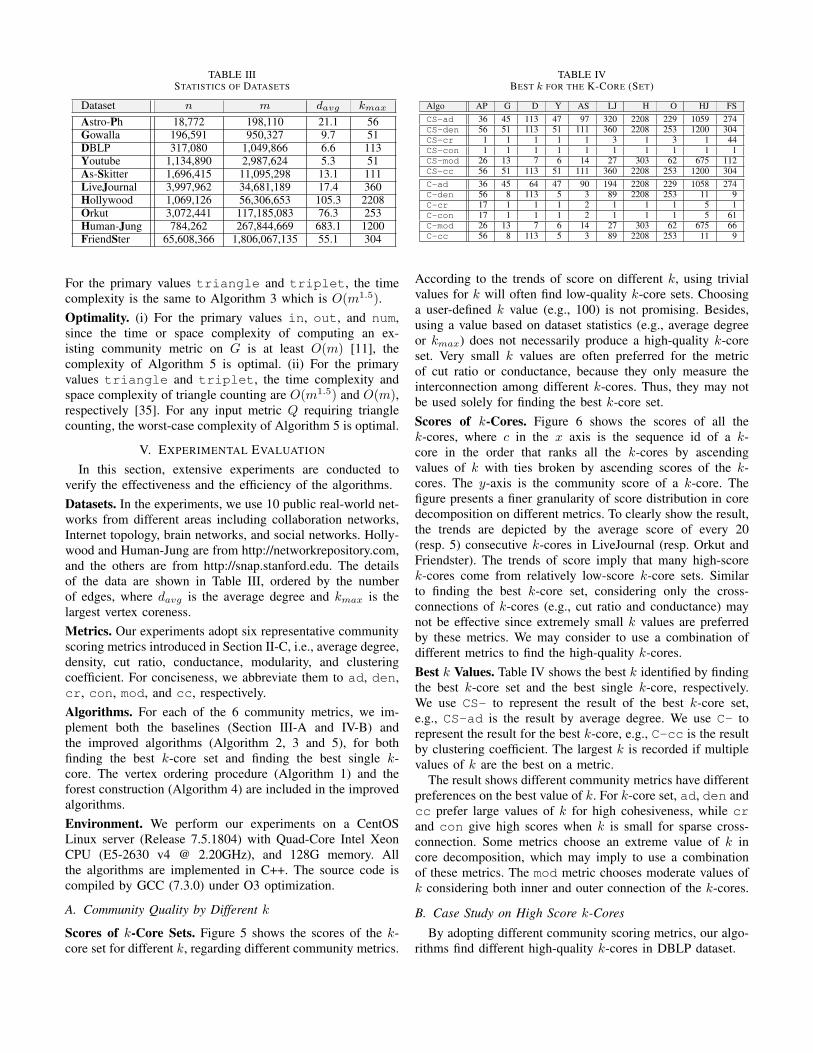
TABLE IIISTATISTICS OF DATASETS
Dataset n m davg kmax
Astro-Ph 18,772 198,110 21.1 56Gowalla 196,591 950,327 9.7 51DBLP 317,080 1,049,866 6.6 113Youtube 1,134,890 2,987,624 5.3 51As-Skitter 1,696,415 11,095,298 13.1 111LiveJournal 3,997,962 34,681,189 17.4 360Hollywood 1,069,126 56,306,653 105.3 2208Orkut 3,072,441 117,185,083 76.3 253Human-Jung 784,262 267,844,669 683.1 1200FriendSter 65,608,366 1,806,067,135 55.1 304
For the primary values triangle and triplet, the timecomplexity is the same to Algorithm 3 which is O(m1.5).Optimality. (i) For the primary values in, out, and num,since the time or space complexity of computing an ex-isting community metric on G is at least O(m) [11], thecomplexity of Algorithm 5 is optimal. (ii) For the primaryvalues triangle and triplet, the time complexity andspace complexity of triangle counting are O(m1.5) and O(m),respectively [35]. For any input metric Q requiring trianglecounting, the worst-case complexity of Algorithm 5 is optimal.
V. EXPERIMENTAL EVALUATION
In this section, extensive experiments are conducted toverify the effectiveness and the efficiency of the algorithms.Datasets. In the experiments, we use 10 public real-world net-works from different areas including collaboration networks,Internet topology, brain networks, and social networks. Holly-wood and Human-Jung are from http://networkrepository.com,and the others are from http://snap.stanford.edu. The detailsof the data are shown in Table III, ordered by the numberof edges, where davg is the average degree and kmax is thelargest vertex coreness.Metrics. Our experiments adopt six representative communityscoring metrics introduced in Section II-C, i.e., average degree,density, cut ratio, conductance, modularity, and clusteringcoefficient. For conciseness, we abbreviate them to ad, den,cr, con, mod, and cc, respectively.Algorithms. For each of the 6 community metrics, we im-plement both the baselines (Section III-A and IV-B) andthe improved algorithms (Algorithm 2, 3 and 5), for bothfinding the best k-core set and finding the best single k-core. The vertex ordering procedure (Algorithm 1) and theforest construction (Algorithm 4) are included in the improvedalgorithms.Environment. We perform our experiments on a CentOSLinux server (Release 7.5.1804) with Quad-Core Intel XeonCPU (E5-2630 v4 @ 2.20GHz), and 128G memory. Allthe algorithms are implemented in C++. The source code iscompiled by GCC (7.3.0) under O3 optimization.
A. Community Quality by Different k
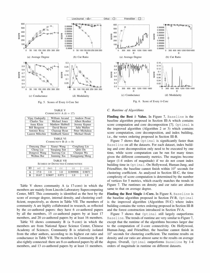
Scores of k-Core Sets. Figure 5 shows the scores of the k-core set for different k, regarding different community metrics.
TABLE IVBEST k FOR THE K-CORE (SET)
Algo AP G D Y AS LJ H O HJ FSCS-ad 36 45 113 47 97 320 2208 229 1059 274CS-den 56 51 113 51 111 360 2208 253 1200 304CS-cr 1 1 1 1 1 3 1 3 1 44CS-con 1 1 1 1 1 1 1 1 1 1CS-mod 26 13 7 6 14 27 303 62 675 112CS-cc 56 51 113 51 111 360 2208 253 1200 304C-ad 36 45 64 47 90 194 2208 229 1058 274C-den 56 8 113 5 3 89 2208 253 11 9C-cr 17 1 1 1 2 1 1 1 5 1C-con 17 1 1 1 2 1 1 1 5 61C-mod 26 13 7 6 14 27 303 62 675 66C-cc 56 8 113 5 3 89 2208 253 11 9
According to the trends of score on different k, using trivialvalues for k will often find low-quality k-core sets. Choosinga user-defined k value (e.g., 100) is not promising. Besides,using a value based on dataset statistics (e.g., average degreeor kmax) does not necessarily produce a high-quality k-coreset. Very small k values are often preferred for the metricof cut ratio or conductance, because they only measure theinterconnection among different k-cores. Thus, they may notbe used solely for finding the best k-core set.Scores of k-Cores. Figure 6 shows the scores of all thek-cores, where c in the x axis is the sequence id of a k-core in the order that ranks all the k-cores by ascendingvalues of k with ties broken by ascending scores of the k-cores. The y-axis is the community score of a k-core. Thefigure presents a finer granularity of score distribution in coredecomposition on different metrics. To clearly show the result,the trends are depicted by the average score of every 20(resp. 5) consecutive k-cores in LiveJournal (resp. Orkut andFriendster). The trends of score imply that many high-scorek-cores come from relatively low-score k-core sets. Similarto finding the best k-core set, considering only the cross-connections of k-cores (e.g., cut ratio and conductance) maynot be effective since extremely small k values are preferredby these metrics. We may consider to use a combination ofdifferent metrics to find the high-quality k-cores.Best k Values. Table IV shows the best k identified by findingthe best k-core set and the best single k-core, respectively.We use CS- to represent the result of the best k-core set,e.g., CS-ad is the result by average degree. We use C- torepresent the result for the best k-core, e.g., C-cc is the resultby clustering coefficient. The largest k is recorded if multiplevalues of k are the best on a metric.
The result shows different community metrics have differentpreferences on the best value of k. For k-core set, ad, den andcc prefer large values of k for high cohesiveness, while crand con give high scores when k is small for sparse cross-connection. Some metrics choose an extreme value of k incore decomposition, which may imply to use a combinationof these metrics. The mod metric chooses moderate values ofk considering both inner and outer connection of the k-cores.
B. Case Study on High Score k-Cores
By adopting different community scoring metrics, our algo-rithms find different high-quality k-cores in DBLP dataset.
LiveJournal Orkut FriendSter
0
100
200
300
400
500
600
0 50 100 150 200 250 300 350
sco
re
k
(a) Average Degree
0.9998
0.99982
0.99984
0.99986
0.99988
0.9999
0.99992
0.99994
0.99996
0.99998
1
0 50 100 150 200 250 300 350
sco
re
k
(b) Cut Ratio
0.3
0.4
0.5
0.6
0.7
0.8
0.9
1
0 50 100 150 200 250 300 350
sco
re
k
(c) Conductance
0
0.05
0.1
0.15
0.2
0.25
0.3
0 50 100 150 200 250 300 350
score
k
(d) Modularity
Fig. 5. Scores of Every k-Core Set
0
100
200
300
400
500
600
0 300 600 900 1200 1500 1800
sco
re
c
(a) Average Degree
0.99982
0.99984
0.99986
0.99988
0.9999
0.99992
0.99994
0.99996
0.99998
1
0 300 600 900 1200 1500 1800
sco
re
c
(b) Cut Ratio
0.3
0.4
0.5
0.6
0.7
0.8
0.9
1
0 300 600 900 1200 1500 1800
sco
re
c
(c) Conductance
0
0.02
0.04
0.06
0.08
0.1
0.12
0.14
0.16
0 300 600 900 1200 1500 1800
sco
re
c
(d) Modularity
Fig. 6. Score of Every k-Core
TABLE VCOMMUNITY A (k = 17)
Vijay Gadepally William Arcand Andrew ProutCharles Yee Michael Jones Albert ReutherAnna Klein Matthew Hubbell Jeremy Kepner
Bill Bergeron David Bestor Julie MullenAntonio Rosa Chansup Byun Peter Michaleas
Lauren Milechin Siddharth Samsi Michael Houle
TABLE VICOMMUNITY B (k = 9)
Danyang Zhao Xianyi Wang Congliang LiuCheng Liu Yueqiang Sun Qifei Du
Dongwei Wang Yuerong Cai Chunjun WuWeihua Bai Junming Xia Xiangguang Meng
TABLE VIISCORES OF DETECTED COMMUNITIES
ID ad den cc cr con
A 17.0 1.0 1.0 0.999998 0.9871B 10.67 0.9697 0.971 1.0 1.0
Table V shows community A (a 17-core) in which themembers are mainly from Lincoln Laboratory SupercomputingCenter, MIT. This community is identified as the best by thescore of average degree, internal density, and clustering coef-ficient, respectively, as shown in Table VII. The members ofcommunity A are highly collaborated in research, as reflectedby the co-authored papers: they have 6 co-authored papersby all the members, 15 co-authored papers by at least 17members, and 20 co-authored papers by at least 16 members.
Table VI shows community B (a 9-core) in which themembers are from National Space Science Center, ChineseAcademy of Sciences. Community B is relatively isolatedfrom the other authors, according to its highest cut ratio andconductance in Table VII. The members in Community B arealso tightly connected: there are 8 co-authored papers by all themembers, and 13 co-authored papers by at least 11 members.
C. Runtime of Algorithms
Finding the Best k Value. In Figure 7, Baseline is thebaseline algorithm proposed in Section III-A which containsscore computation and core decomposition [7]. Optimal isthe improved algorithm (Algorithm 2 or 3) which containsscore computation, core decomposition, and index building,i.e., the vertex ordering proposed in Section III-B.
Figure 7 shows that Optimal is significantly faster thanBaseline on all the datasets. For each dataset, index build-ing and core decomposition only need to be executed by onetime, while score computation can be run for many timesgiven the different community metrics. The margins becomelarger (1-4 orders of magnitude) if we do not count indexbuilding time in Optimal. On Hollywood, Human-Jung, andFriendSter, the baseline cannot finish within 105 seconds forclustering coefficient. As analyzed in Section III-C, the timecomplexity of score computation is determined by the numberof vertices for 5 metrics, which exactly matches the trends inFigure 7. The runtimes on density and cur ratio are almostsame to that on average degree.Finding the Best Single k-Core. In Figure 8, Baseline isthe baseline algorithm proposed in Section IV-B, Optimalis the improved algorithm (Algorithm IV-C) where indexbuilding contains the vertex ordering proposed in Section III-Band the forest construction introduced in Section IV-A.
Figure 7 shows that Optimal still largely outperformsBaseline. The trends of runtime are very similar to Figure 7,except that the runtime of the algorithms becomes larger dueto the computation of k-core connectivity. On Hollywood,Human-Jung, and FriendSter, the baseline cannot finish in105 seconds for clustering coefficient. The runtime results ondensity and cur ratio are almost same to the results on averagedegree. Overall, Optimal outperforms Baseline by 1-4orders of magnitude in runtime on different datasets.

+ index building + core decomposition
= baseline score computationBaseline
Optimal = our score computation
+ core decomposition
1ms10ms
100ms1s
10s100s
103104105
AP G D Y AS LJ H O HJ FS1ms
10ms100ms
1s10s
100s103104105
AP G D Y AS LJ H O HJ FS
(a) Average Degree
1ms10ms
100ms1s
10s100s
103104105
AP G D Y AS LJ H O HJ FS1ms
10ms100ms
1s10s
100s103104105
AP G D Y AS LJ H O HJ FS
(b) Conductance
1ms10ms
100ms1s
10s100s
103104105
AP G D Y AS LJ H O HJ FS1ms
10ms100ms
1s10s
100s103104105
AP G D Y AS LJ H O HJ FS
(c) Modularity
1ms10ms
100ms1s
10s100s
103104105
AP G D Y AS LJ H O HJ FS1ms
10ms100ms
1s10s
100s103104105
AP G D Y AS LJ H O HJ FS
(d) Clustering Coefficient
Fig. 7. Performance of Finding the Best k-Core Set
1ms10ms
100ms1s
10s100s
103104105
AP G D Y AS LJ H O HJ FS1ms
10ms100ms
1s10s
100s103104105
AP G D Y AS LJ H O HJ FS
(a) Average Degree
1ms10ms
100ms1s
10s100s
103104105
AP G D Y AS LJ H O HJ FS1ms
10ms100ms
1s10s
100s103104105
AP G D Y AS LJ H O HJ FS
(b) Conductance
1ms10ms
100ms1s
10s100s
103104105
AP G D Y AS LJ H O HJ FS1ms
10ms100ms
1s10s
100s103104105
AP G D Y AS LJ H O HJ FS
(c) Modularity
1ms10ms
100ms1s
10s100s
103104105
AP G D Y AS LJ H O HJ FS1ms
10ms100ms
1s10s
100s103104105
AP G D Y AS LJ H O HJ FS
(d) Clustering Coefficient
Fig. 8. Performance of Finding the Best Single k-Core
D. Application on Other ProblemsIn this experiment, we investigate the application of our
algorithm on 3 problems related to k-core, i.e., finding densestsubgraph, maximum clique and size-constrained k-core. Notethat the above problems are all NP-hard. In the following,we show that our algorithm can serve as better approximatesolutions compared with the state-of-the-art, or produce usefulintermediate results. Let Opt-D denote our algorithm whichreturns the best k-core regarding average degree (Algorithm5). Let S∗ denote the output of Opt-D.Densest Subgraph. The densest subgraph (DS) problem is tofind the subgraph with the largest average vertex degree [26].Our Opt-D produces a 1
2 -approximate solution for DS prob-lem, because the kmax-core is one of our candidate results,which is a 1
2 -approximate solution [26]. We compare Opt-Dwith the recent approximate solution named CoreApp [26]which is the fastest algorithm for DS problem. As shownin Table VIII, Opt-D outperforms CoreApp in both outputquality (average degree) and runtime on most datasets. Notethat the better values in Table VIII are marked in bold.Maximum Clique. The maximum clique (MC) problem isto find the largest subset of vertices such that every pair ofvertices in the subset is adjacent [12]. As shown in Table VIII,it is likely that S∗ contains the maximum clique (6 out of 10datasets), although S∗ is not large (the proportion of S∗ in thewhole vertex set is often within 1%). This finding can benefitthe algorithm design for MC problem.Size-Constrained k-Core. Given an integer k, an integer h,and a query vertex v, the query of size-constrained k-core(SCK) is to find a k-core of size h which contains v. Basedon the average degree of every k-core computed by Opt-D,the algorithm Opt-SC first selects the k′-core S′ that has thehighest average degree, where (i) k′ ≥ k (ii) S′ contains v;and (iii) |V (S′)| ≥ h. Then, Opt-SC peels S′ to find more
TABLE VIIIPERFORMANCE OF Opt-D ON DENSEST SUBGRAPH & MAXIMUM CLIQUE
DatasetCoreApp Opt-D Opt-D (output S∗)
davg time (s) davg time (s) MC ⊆ S∗ |S∗|/nAP 56.035 0.11 58.923 0.02 X 7.87%G 76 0.195 87.593 0.093 0.28%D 113 0.233 113.13 0.138 X 0.04%Y 86.066 0.594 91.1 0.498 X 0.18%AS 150.018 1.145 178.801 1.374 0.03%LJ 374.71 4.943 387.027 4.832 X 0.01%H 2208 3.002 2208 3.635 X 0.21%O 438.64 20.14 455.732 11.72 0.85%HJ 2013.879 15.272 2114.915 14.457 X 1.15%FS 513.852 1041.528 547.035 836.279 0.08%
S∗ is the output of Opt-D. davg is the average degree of the output.MC ⊆ S∗ means the maximum clique is contained in S∗. |S∗|/n is
the vertex proportion of S∗ in the whole graph.
TABLE IXPERFORMANCE OF Opt-SC ON SIZE-CONSTRAINED k-CORE (DBLP)
c(v) k = 10 k = 15 k = 20 k = 30 k = 4030 96.45% 88.31% 76.21% 20.97% /43 97.46% 91.41% 82.10% 37.87% 6.69%51 99.12% 96.75% 92.64% 49.81% 30.77%64 98.61% 95.15% 89.62% 61.88% 57.86%
113 98.61% 95.15% 89.62% 61.88% 57.86%
Given a random query point v with coreness c(v), the percentage thatOpt-SC returns a k-core with at most 5% size deviation to h.
results (k-cores) until |V (S′)| ≤ h: in each step of the peeling,it removes the vertex with the lowest degree (skip v) and thevertices with degree less than k in S′.
Table IX shows the performance of Opt-SC on DBLP. Wesay Opt-SC hits a query if the returned k-core contains v andhas at most 5% size deviation to h. Opt-SC is very likelyto hit the query when c(v) is larger than k. Note that somecoreness values do not exist, i.e., no vertex has such coreness.As the time complexity of Opt-SC is linear to graph size, itcan benefit the algorithm design for SCK problem.
VI. DISCUSSIONS AND FUTURE WORK
In this section, we explore several future extensions of ourproposed models and algorithms.
A. Other Community MetricsThere are various existing community scoring metrics and
many potential new metrics by combining the existing ones oradopting new structure properties. Our algorithms can handlemost community metrics based on the studied 5 primary valuesin Section II-C. A survey of community metrics [11] organizesand reviews many existing metrics where the majority (suitablefor core decomposition) are based on the above 5 primaryvalues. The exceptions include some metrics based on higher-order motifs [5], some metrics for overlapped communities,etc. They are interesting for further study.
B. Other Hierarchical DecompositionsIf a cohesive subgraph model with input k has the con-
tainment property, i.e., the (k + 1)-subgraph is always asubgraph of the k-subgraph, our algorithm for finding thebest k may be applied to find the best k. When the foreststructure of a hierarchical decomposition is similar to that ofcore decomposition in Section IV-A, our algorithm for findingthe best single k-core is also applicable.
For instance, our algorithms can shed light on the solutionson the decomposition of k-truss. To find the best k-truss set,we may rank the incident edges of every vertex by theirtruss numbers and record some position tags, to facilitate theincremental score computation. Given the score of (k + 1)-truss set S, to compute the score for k-truss set, we canvisit the vertices in k-truss set but not in S, and additionalvertices incident to edges with truss number k. The solutionfor computing the best single k-truss can be derived similarly,while designing an optimal solution is still challenging.
VII. RELATED WORK
Diverse models of cohesive subgraph are proposed toaccommodate different scenarios, for example, clique [17],quasi-clique [47], k-core [7], [33], [51], k-truss [19], [31],[56], k-plex [58], and k-ecc [13], [68]. Some cohesive sub-graph models decompose a graph into hierarchical structure,e.g., core decomposition [43], [61], truss decomposition [52],[56], [67], and ecc decomposition [13], [64]. Core decom-position is one of the most well-studied models, due toits effectiveness in various applications including communitydiscovery [15], [16], [28], [38], [39], influential spreaderidentification [24], [34], [40], [41], network analysis [4], [21],[30], [53], anomaly detection [53], evaluating contagion powerof vertices [34], [55], and graph visualization [3], [20], [67].
An O(m) time in-memory algorithm for core decompositionis proposed in [7]. The construction of core forest can also becomputed in O(m) time [42]. The core decomposition underdistributed configuration is introduced in [43]. An I/O efficientalgorithm for core decomposition is proposed in [61]. Variousvariants of k-core are explored, including (k, r)-core [65],diversified coherent k-core [69], and skyline k-core [38].
The model of k-core is extended to weighted graphs whereeach edge has its weight and each vertex has its weighted
degree, as introduced in [23], [27], [60]. The weighted coredecomposition can be applied to evaluate the cooperation ink-core communities [29] and identify influential spreaders [1].The techniques for k-core computation and decompositioncannot be applied to solve our problem, because the priorworks only aim to find all the k-core structures and do notcompute the score of any k-core. Our algorithm may shed lighton finding the best k-core on weighted graphs if we apply theweighted community scores. For the problem of extractinga dense subgraph, there is a solution that aims to find thesubgraph S such that fα(S) = m(S)−α
(n(S)
2
)is maximized,
while the subgraph S is not guaranteed to be a k-core, andthe techniques cannot be used to solve our problems [54].
Metrics for community evaluation are surveyed in [11], [63]such as modularity [9], [45] and clustering coefficient [32],[49]. Community scoring metrics can be used to effectivelycompare the communities produced by different algorithms,and formalize the notion of network communities [37]. Dif-ferent communities can be found by the optimization guidedby different community metrics, e.g., [2], [14], [18], [62]. Tothe best of our knowledge, this paper is the first attempt toapply community scoring metrics to compute the quality ofk-cores and other cohesive subgraph models such as k-truss.
VIII. CONCLUSION
In this paper, we study the problems of computing the bestk-core set and the best single k-core with respect to a commu-nity scoring metric. Since there are various metrics consideringdifferent standards, we focus on 5 common primary valuesto handle different metrics. Benefitting from a light-weightvertex ordering procedure with O(m) time complexity, wepropose time and space optimal algorithms for the studiedproblems. We conduct extensive experiments on 10 real-worldgraphs with size up to billion-scale, where our algorithms notonly significantly outperform the baselines in runtime but alsoprovide profound insights for the related problems.
ACKNOWLEDGMENTS
Xuemin Lin is supported by 2018YFB1003504, NSFC61232006, ARC DP180103096 and DP170101628. Wenjie Zhangis supported by ARC DP180103096. Ying Zhang is supportedby ARC DP180103096 and FT170100128.
REFERENCES
[1] M. A. Al-garadi, K. D. Varathan, and S. D. Ravana. Identification ofinfluential spreaders in online social networks using interaction weightedk-core decomposition method. Physica A, 468:278–288, 2017.
[2] D. Aloise, G. Caporossi, P. Hansen, L. Liberti, S. Perron, and M. Ruiz.Modularity maximization in networks by variable neighborhood search.In Graph Partitioning and Graph Clustering, pages 113–128, 2012.
[3] J. I. Alvarez-Hamelin, L. Dall’Asta, A. Barrat, and A. Vespignani.Large scale networks fingerprinting and visualization using the k-coredecomposition. In NIPS, pages 41–50, 2005.
[4] J. I. Alvarez-Hamelin, L. Dall’Asta, A. Barrat, and A. Vespignani. K-core decomposition of internet graphs: hierarchies, self-similarity andmeasurement biases. NHM, 3(2):371–393, 2008.
[5] A. Arenas, A. Fernandez, S. Fortunato, and S. Gomez. Motif-basedcommunities in complex networks. Journal of Physics A: Mathematicaland Theoretical, 41(22):224001, 2008.
[6] G. D. Bader and C. W. V. Hogue. An automated method for findingmolecular complexes in large protein interaction networks. BMCBioinformatics, 4:2, 2003.
[7] V. Batagelj and M. Zaversnik. An o(m) algorithm for cores decompo-sition of networks. CoRR, cs.DS/0310049, 2003.
[8] M. Bola and B. A. Sabel. Dynamic reorganization of brain functionalnetworks during cognition. Neuroimage, 114:398–413, 2015.
[9] U. Brandes, D. Delling, M. Gaertler, R. Gorke, M. Hoefer, Z. Nikoloski,and D. Wagner. On modularity clustering. TKDE, 20(2):172–188, 2008.
[10] S. Carmi, S. Havlin, S. Kirkpatrick, Y. Shavitt, and E. Shir. A model ofinternet topology using k-shell decomposition. PNAS, 104(27):11150–11154, 2007.
[11] T. Chakraborty, A. Dalmia, A. Mukherjee, and N. Ganguly. Metrics forcommunity analysis: A survey. ACM Comput. Surv., 50(4):54:1–54:37,2017.
[12] L. Chang. Efficient maximum clique computation over large sparsegraphs. In KDD, pages 529–538, 2019.
[13] L. Chang, J. X. Yu, L. Qin, X. Lin, C. Liu, and W. Liang. Efficientlycomputing k-edge connected components via graph decomposition. InSIGMOD, pages 205–216, 2013.
[14] C. Chen, R. Peng, L. Ying, and H. Tong. Network connectivityoptimization: Fundamental limits and effective algorithms. In KDD,pages 1167–1176, 2018.
[15] L. Chen, C. Liu, K. Liao, J. Li, and R. Zhou. Contextual communitysearch over large social networks. In ICDE, pages 88–99, 2019.
[16] L. Chen, C. Liu, R. Zhou, J. Li, X. Yang, and B. Wang. Maximumco-located community search in large scale social networks. PVLDB,11(10):1233–1246, 2018.
[17] J. Cheng, Y. Ke, A. W. Fu, J. X. Yu, and L. Zhu. Finding maximalcliques in massive networks. ACM Trans. Database Syst., 36(4):21:1–21:34, 2011.
[18] A. Clauset. Finding local community structure in networks. Physicalreview E, 72(2):026132, 2005.
[19] J. Cohen. Trusses: Cohesive subgraphs for social network analysis.National Security Agency Technical Report, 16:3–1, 2008.
[20] P. Colomer-de-Simon, M. A. Serrano, M. G. Beiro, J. I. Alvarez-Hamelin, and M. Boguna. Deciphering the global organization ofclustering in real complex networks. CoRR, abs/1306.0112, 2013.
[21] M. Daianu, N. Jahanshad, T. M. Nir, A. W. Toga, C. R. J. Jr., M. W.Weiner, and P. M. Thompson. Breakdown of brain connectivity betweennormal aging and alzheimer’s disease: A structural k-core networkanalysis. Brain Connectivity, 3(4):407–422, 2013.
[22] Y. Dourisboure, F. Geraci, and M. Pellegrini. Extraction and classifica-tion of dense implicit communities in the web graph. TWEB, 3(2):7:1–7:36, 2009.
[23] M. Eidsaa and E. Almaas. S-core network decomposition: A general-ization of k-core analysis to weighted networks. Physical Review E,88(6):062819, 2013.
[24] S. Elsharkawy, G. Hassan, T. Nabhan, and M. Roushdy. Effectivenessof the k-core nodes as seeds for influence maximisation in dynamiccascades. International Journal of Computers, 2, 2017.
[25] Y. Fang, R. Cheng, X. Li, S. Luo, and J. Hu. Effective communitysearch over large spatial graphs. PVLDB, 10(6):709–720, 2017.
[26] Y. Fang, K. Yu, R. Cheng, L. V. S. Lakshmanan, and X. Lin. Efficientalgorithms for densest subgraph discovery. PVLDB, 12(11):1719–1732,2019.
[27] A. Garas, F. Schweitzer, and S. Havlin. A k-shell decomposition methodfor weighted networks. New Journal of Physics, 14(8):083030, 2012.
[28] C. Giatsidis, F. D. Malliaros, D. M. Thilikos, and M. Vazirgiannis.Corecluster: A degeneracy based graph clustering framework. In AAAI,pages 44–50, 2014.
[29] C. Giatsidis, D. M. Thilikos, and M. Vazirgiannis. Evaluating coop-eration in communities with the k-core structure. In ASONAM, pages87–93, 2011.
[30] L. Hebert-Dufresne, A. Allard, J.-G. Young, and L. J. Dube. Percolationon random networks with arbitrary k-core structure. Physical Review E,88(6):062820, 2013.
[31] X. Huang, H. Cheng, L. Qin, W. Tian, and J. X. Yu. Querying k-trusscommunity in large and dynamic graphs. In SIGMOD, pages 1311–1322, 2014.
[32] L. Katzir and S. J. Hardiman. Estimating clustering coefficients and sizeof social networks via random walk. TWEB, 9(4):19:1–19:20, 2015.
[33] W. Khaouid, M. Barsky, S. Venkatesh, and A. Thomo. K-core decom-position of large networks on a single PC. PVLDB, 9(1):13–23, 2015.
[34] M. Kitsak, L. K. Gallos, S. Havlin, F. Liljeros, L. Muchnik, H. E.Stanley, and H. A. Makse. Identification of influential spreaders incomplex networks. Nature physics, 6(11):888, 2010.
[35] M. Latapy. Main-memory triangle computations for very large (sparse(power-law)) graphs. Theor. Comput. Sci., 407(1-3):458–473, 2008.
[36] J. Leskovec and A. Krevl. SNAP Datasets: Stanford large networkdataset collection. http://snap.stanford.edu/data, June 2014.
[37] J. Leskovec, K. J. Lang, and M. W. Mahoney. Empirical comparison ofalgorithms for network community detection. In WWW, pages 631–640,2010.
[38] R. Li, L. Qin, F. Ye, J. X. Yu, X. Xiao, N. Xiao, and Z. Zheng. Skylinecommunity search in multi-valued networks. In SIGMOD, pages 457–472, 2018.
[39] R. Li, J. Su, L. Qin, J. X. Yu, and Q. Dai. Persistent community searchin temporal networks. In ICDE, pages 797–808, 2018.
[40] J.-H. Lin, Q. Guo, W.-Z. Dong, L.-Y. Tang, and J.-G. Liu. Identifyingthe node spreading influence with largest k-core values. Physics LettersA, 378(45):3279–3284, 2014.
[41] F. D. Malliaros, M.-E. G. Rossi, and M. Vazirgiannis. Locatinginfluential nodes in complex networks. Scientific reports, 6:19307, 2016.
[42] D. W. Matula and L. L. Beck. Smallest-last ordering and clustering andgraph coloring algorithms. J. ACM, 30(3):417–427, 1983.
[43] A. Montresor, F. D. Pellegrini, and D. Miorandi. Distributed k-coredecomposition. IEEE TPDS, 24(2):288–300, 2013.
[44] F. Morone, G. Del Ferraro, and H. A. Makse. The k-core as a predictor ofstructural collapse in mutualistic ecosystems. Nature Physics, 15(1):95,2019.
[45] M. E. Newman. Modularity and community structure in networks.PNAS, 103(23):8577–8582, 2006.
[46] M. E. Newman and M. Girvan. Finding and evaluating communitystructure in networks. Physical review E, 69(2):026113, 2004.
[47] J. Pei, D. Jiang, and A. Zhang. On mining cross-graph quasi-cliques.In KDD, pages 228–238, 2005.
[48] R. A. Rossi and N. K. Ahmed. The network data repository withinteractive graph analytics and visualization. In Proceedings of theTwenty-Ninth AAAI Conference on Artificial Intelligence, 2015.
[49] J. Saramaki, M. Kivela, J.-P. Onnela, K. Kaski, and J. Kertesz. Gen-eralizations of the clustering coefficient to weighted complex networks.Physical Review E, 75(2):027105, 2007.
[50] A. E. Sariyuce and A. Pinar. Fast hierarchy construction for densesubgraphs. PVLDB, 10(3):97–108, 2016.
[51] S. B. Seidman. Network structure and minimum degree. Social networks,5(3):269–287, 1983.
[52] Y. Shao, L. Chen, and B. Cui. Efficient cohesive subgraphs detectionin parallel. In SIGMOD, pages 613–624, 2014.
[53] K. Shin, T. Eliassi-Rad, and C. Faloutsos. Corescope: Graph miningusing k-core analysis - patterns, anomalies and algorithms. In ICDM,pages 469–478, 2016.
[54] C. E. Tsourakakis, F. Bonchi, A. Gionis, F. Gullo, and M. A. Tsiarli.Denser than the densest subgraph: extracting optimal quasi-cliques withquality guarantees. In KDD, pages 104–112, 2013.
[55] J. Ugander, L. Backstrom, C. Marlow, and J. Kleinberg. Structuraldiversity in social contagion. PNAS, 109(16):5962–5966, 2012.
[56] J. Wang and J. Cheng. Truss decomposition in massive networks.PVLDB, 5(9):812–823, 2012.
[57] K. Wang, X. Cao, X. Lin, W. Zhang, and L. Qin. Efficient computingof radius-bounded k-cores. In ICDE, pages 233–244, 2018.
[58] Y. Wang, X. Jian, Z. Yang, and J. Li. Query optimal k-plex basedcommunity in graphs. DSE, 2(4):257–273, 2017.
[59] D. J. Watts and S. H. Strogatz. Collective dynamics of ‘small-world’networks. Nature, 393(6684):440, 1998.
[60] B. Wei, J. Liu, D. Wei, C. Gao, and Y. Deng. Weighted k-shelldecomposition for complex networks based on potential edge weights.Physica A, 420:277–283, 2015.
[61] D. Wen, L. Qin, Y. Zhang, X. Lin, and J. X. Yu. I/O efficient core graphdecomposition at web scale. In ICDE, pages 133–144, 2016.
[62] Y. Wu, R. Jin, J. Li, and X. Zhang. Robust local community detection:On free rider effect and its elimination. PVLDB, 8(7):798–809, 2015.
[63] J. Yang and J. Leskovec. Defining and evaluating network communitiesbased on ground-truth. Knowl. Inf. Syst., 42(1):181–213, 2015.
[64] L. Yuan, L. Qin, X. Lin, L. Chang, and W. Zhang. I/O efficient ECCgraph decomposition via graph reduction. VLDB J., 26(2):275–300,2017.
[65] F. Zhang, Y. Zhang, L. Qin, W. Zhang, and X. Lin. When engagementmeets similarity: Efficient (k, r)-core computation on social networks.PVLDB, 10(10):998–1009, 2017.
[66] H. Zhang, H. Zhao, W. Cai, J. Liu, and W. Zhou. Using the k-coredecomposition to analyze the static structure of large-scale softwaresystems. The Journal of Supercomputing, 53(2):352–369, 2010.
[67] F. Zhao and A. K. H. Tung. Large scale cohesive subgraphs discoveryfor social network visual analysis. PVLDB, 6(2):85–96, 2012.

[68] R. Zhou, C. Liu, J. X. Yu, W. Liang, B. Chen, and J. Li. Findingmaximal k-edge-connected subgraphs from a large graph. In EDBT,pages 480–491, 2012.
[69] R. Zhu, Z. Zou, and J. Li. Diversified coherent core search on multi-layer graphs. In ICDE, pages 701–712, 2018.