fine mapping of resistance against root aphids in sugar beet · kromosom i på sockerbeta, men...

Collaboration with Syngenta Seeds AB

The Faculty of Landscape Planning, Horticulture and Agriculture Science

Självständigt arbete vid LTJ-fakulteten, SLU, Alnarp Master thesis in Biology, Horticulture Programme

Alnarp, 2011

Fine mapping of resistance against root

aphids in sugar beet

Emma Leijman

SLU, Swedish University of Agricultural Sciences The Faculty of Landscape Planning, Horticulture and Agriculture

The Department of Plant Breeding and Biotechnology

Author Emma Leijman

English title Fine mapping of resistance against root aphids in sugar beet

Swedish title Finkartering av resistens mot rotlöss hos sockerbeta

Keywords resistance, sequencing, mapping, molecular marker, single-

nucleotide polymorphism, SNP, genome sequence,

breeding, root aphids, Pemphigus betae, sugar beet

Supervisor Associate Professor Inger Åhman, Swedish University of

Agricultural Sciences, Plant Breeding and Biotechnology

Associate supervisor PhD Thomas Kraft, Head of Sugar Beet Bioscience at

Syngenta Seeds AB, Landskrona

Examiner PhD Larisa Gustavsson, SLU, Plant Breeding and

Biotechnology

Programme Horticulture programme

Course title Degree Project for MSc Thesis in Horticulture

Course code EX0544

Subject Biology

Credits 30 HEC

Level A2E

Självständigt arbete vid LTJ-fakulteten, SLU

Alnarp, 2011 Cover illustration by Emma Leijman All photos and illustrations are the property of the author, unless otherwise stated

Acknowledgements This master thesis took its first step in January 2011 and for its realization I have many

people to thank. First and foremost this project would not have been possible to accomplish

without the collaboration with Syngenta Seeds, thus thanks to PhD Thomas Kraft, my

associate supervisor and the head of sugar beet bioscience at Syngenta in Landskrona, and

to PhD Britt-Louise Lennefors, group leader of the pathology department at Syngenta in

Landskrona, for giving me the opportunity to write my thesis at Syngenta. Many thanks to all

of the wonderful people working at the Molecular and Pathology department at Syngenta in

Landskrona for the warm welcome I received on my first day and for giving me a helping

hand when I have needed it. I have to give a special thank to two persons who have helped

me tremendously during these five months; to PhD student Pierre Pin for your guiding

through a world of molecular markers and to MSc Louise Andersson for your dedication to

the phenotypic test and to both of you for taking the time to answer my questions.

Thanks to PhD Jeff Bradshaw at the University of Nebraska-Lincoln for sharing your

expertise on sugar beet root aphids and for providing us with aphids.

Also thanks to Associate Professor Inger Åhman for being my supervisor and to PhD Larisa

Gustavsson for being my examiner.

Last, but certainly not the least; many thanks to my wonderful John and my amazing family

for always supporting and believing in me!

2

Abstract Sugar beet, Beta vulgaris, is an important crop for the global sugar industry being one of the

two major crops cultivated for sugar production. In the USA, the sugar beet root aphid,

Pemphigus betae, is a regionally occurring pest which damages sugar beets by feeding on

their secondary roots which results in reduced biomass and hence a lower yield. To date, the

best alternative to control the aphids is by use of resistant varieties. To find such resistance

and to introduce it in plant material by plant breeding it is necessary to have a precise and fast

selection method for the resistance. In modern plant breeding more and more of useful plant

characteristics are selected for via molecular markers.

A locus on sugar beet chromosome I is known to harbor resistance to the root aphid, but

the markers flanking the locus were too far from the actual gene(s) to be really useful for

selections. The aim of this master thesis was to fine map the resistance locus by means of

sequencing to enable identification of SNPs in close proximity of the locus and by conducting

a phenotypic test under greenhouse conditions.

The phenotypic test showed varying results, but was still a useful complement to the

marker analysis. Several lines scored fairly consistent, while other lines had plants which

scored anything between susceptible and resistant. However, in most cases the results from

the phenotypic test were comparable to earlier phenotypic data from a field test, and part of

the variation was because there still was segregation among sugar beet offspring but most

likely also due to escapes from infestation. Since the phenotypic test was a pilot test there

were some aspects that could be improved, for instance the selection of soil type.

The results from the sequencing showed that nearly 50% of the DNA targets were

polymorphic. The other half of the DNA targets turned out to be either monomorphic or failed

due to technical reasons or difficulties in amplification of the locus. From the fine mapping,

five SNP markers were found in the vicinity of the interval where the resistance locus was

previously mapped, making it possible to narrow down the resistance locus. The

recombination frequency of the two markers closest to the resistance locus was 1.6%.

Although the new markers can be utilized in marker-assisted breeding for the sugar beet root

aphid resistance, recombinant events are still present between the two markers suggesting that

further narrowing-down of the interval would be feasible.

Keywords: resistance, sequencing, mapping, molecular marker, single-nucleotide

polymorphism, SNP, genome sequence, breeding, root aphids, Pemphigus betae, sugar beet

3

Sammanfattning Sockerbeta, Beta vulgaris, är en av två grödor som huvudsakligen odlas för att producera

socker och är därför en viktig gröda inom den globala sockerindustrin. I USA är rotlöss på

sockerbeta, Pemphigus betae, en regionalt förekommande skadegörare som orsakar skador

hos sockerbetan genom att suga ut saften ur deras sekundära rötter vilket resulterar i minskad

biomassa hos sockerbetan och därmed en minskad avkastning. Hittills är resistenta sorter det

bästa alternativet för att bekämpa rotlössen. För att hitta sådan resistens och introducera den i

växtmaterial är det viktigt att ha en precis och snabb selektionsmetod för resistensen. I

modern växtförädling selekteras allt fler plantegenskaper med hjälp av molekylära markörer.

Det är sedan tidigare känt att resistensen mot rotlöss är lokaliserad till ett locus på

kromosom I på sockerbeta, men flankerande markörer ligger för långt ifrån själva genen

(generna) för att vara användbara för att selektera resistenta plantor. Syftet med detta

examensarbete var att finkartera resistenslocuset genom sekvensering och identifiering av

SNPs nära locuset och genom att utföra ett fenotyptest i växthus.

Fenotyptestet uppvisade varierande resultat, men var ändå ett användbart komplement

till marköranalysen. Flera linjer uppvisade ett relativt jämnt resultat, medan andra linjer hade

plantor som var både känsliga och resistenta. Likväl var resultatet från fenotyptestet i de flesta

fall jämförbara med tidigare fenotypdata från ett fältförsök, och variationen berodde delvis på

att där fanns en segregation i avkomman, men mest troligt berodde det även på att en del

plantor inte blivit infekterade. Eftersom fenotyptestet var ett pilottest fanns det en del aspekter

som kan förbättras, t.ex. valet av jordtyp.

Resultaten från sekvenseringen visade att 50 % av DNA-segmenten var polymorfa. Den

andra halvan av DNA-segmenten var antingen monomorfa eller så misslyckades

sekvenseringen på grund av tekniska orsaker eller att amplifiering i locuset är svårt. Vid

finkarteringen hittades fem SNP markörer i närheten av det område där resistenslocuset

tidigare karterats vilket medförde att området för resistensen kunde begränsas.

Rekombinationsfrekvensen för de två markörerna närmast resistenslocuset var 1,6 %. Även

om de nya markörerna kan användas vid markörstödd förädling av resistensen mot rotlöss

finns det fortfarande några rekombinanta linjer mellan de två markörerna vilket indikerar att

det är möjligt att begränsa området för resistensen ytterligare.

Nyckelord: resistens, sekvensering, kartering, molekylär markör, single-nucleotide

polymorphism, SNP, genomsekvens, förädling, rotlöss, Pemphigus betae, sockerbeta

4

Glossary Contig = DNA sequence that, with a high confidence level, corresponds to a part of the

genome

Indel = a mutation resulting in either an insertion or a deletion of one or more nucleotides in

the chromosome

SNP = Single-Nucleotide Polymorphism; refers to a mutation at a single nucleotide position

in the genome

Scaffold = a part of the genome sequence information that is composed of contigs and gaps

5

Contents

Acknowledgements .......................................................................................................................................... 1

Abstract ........................................................................................................................................................... 2

Sammanfattning .............................................................................................................................................. 3

Glossary ........................................................................................................................................................... 4

1. Introduction ............................................................................................................................................. 7

1.1. Sugar beet (Beta vulgaris L.) ..................................................................................................................... 7

1.1.1. Sugar beet production .............................................................................................................. 7

1.1.2. Biology ...................................................................................................................................... 7

1.2. Sugar Beet Root Aphids (Pemphigus betae Doane) .................................................................................. 8

1.2.1. Life cycle and hosts .......................................................................................................................... 8

1.2.2. Damage ............................................................................................................................................ 9

1.2.3. Management ................................................................................................................................. 10

1.3. Resistance ............................................................................................................................................... 10

1.3.1. Plant defense and resistance mechanisms ............................................................................. 11

1.3.2. Resistant varieties .................................................................................................................. 11

1.4. Plant Breeding ......................................................................................................................................... 12

1.4.1. Sugar beet breeding ............................................................................................................... 12

1.5. DNA (deoxyribonucleic acid) markers ..................................................................................................... 13

1.5.1. Different types of DNA markers .............................................................................................. 14

1.5.2. Single-Nucleotide Polymorphism (SNP) .................................................................................. 15

1.5.3. Marker-assisted breeding ....................................................................................................... 16

1.6. Sequencing .............................................................................................................................................. 17

1.7. Aim .......................................................................................................................................................... 18

2. Materials and Methods .......................................................................................................................... 19

2.1. Plant material .......................................................................................................................................... 19

2.1.1. Phenotypic test ....................................................................................................................... 19

2.1.2. Marker analysis ...................................................................................................................... 19

2.2. Insect material ........................................................................................................................................ 20

2.3. Phenotypic test ....................................................................................................................................... 20

2.4. DNA isolation .......................................................................................................................................... 21

2.5. In silico selection of DNA targets ............................................................................................................ 21

2.6. Polymerase chain reaction (PCR) ............................................................................................................ 21

6

2.7. Control of the PCR products ................................................................................................................... 22

2.8. Sequencing and SNP discovery ............................................................................................................... 22

3. Results ................................................................................................................................................... 23

3.1. Phenotypic test ....................................................................................................................................... 23

3.2. Target selection....................................................................................................................................... 25

3.3. Sequencing .............................................................................................................................................. 25

3.4. Fine Mapping .......................................................................................................................................... 27

4. Discussion .............................................................................................................................................. 32

4.1. Phenotypic test ....................................................................................................................................... 32

4.2. Sequencing .............................................................................................................................................. 32

4.3. Fine mapping........................................................................................................................................... 33

5. Conclusions ............................................................................................................................................ 35

6. References ............................................................................................................................................. 36

Appendices .................................................................................................................................................... 42

Appendix I – Control of PCR products ............................................................................................................. 43

Appendix II – Illustration of the phenotypic test ............................................................................................ 44

Appendix III – Scoring of the phenotypic test ................................................................................................. 45

7

1. Introduction

1.1. Sugar beet (Beta vulgaris L.)

1.1.1. Sugar beet production

Sugar beet (Beta vulgaris L.) is a root crop commonly used to extract sugar which is an

important food source. In 1747, the sugar in the roots of the beet was discovered, and in 1784,

different varieties of beets from the genus Beta were studied to compare differences in sugar

production. The first publication on cultivating the crop for sugar production is dated back to

1799 and two years later the first sugar beet factory was established in Cunern, Silesia. Since

1850, systematic selection of beets regarding sugar content has been performed (Cooke &

Scott, 1993).

Today, sugar beet (together with sugarcane) constitutes most of the sugar production in

the world (Biancardi et al., 2005). During the year 2008, sugar beet was the tenth most

cultivated crop in the world with a global production of approximately 220 million tons

(FAOSTAT a). Out of these, Europe accounted for producing approximately 150 million tons,

followed by America and Asia with a production of approximately 30 million tons each and

Africa with a production of approximately 8 million tons. During that same year, North

America and Sweden produced approximately 25 and 2 million tons of sugar beet

respectively (FAOSTAT b, 2011).

1.1.2. Biology

Sugar beet is an herbaceous dicotyledon (Biancardi et al., 2005) belonging to the family

Amaranthaceae (Yamane). With the basic haploid chromosome number x = 9, the crop is a

true diploid (Biancardi et al., 2005). The plant is biennial; that is completing its life cycle in

two years. During the first year, continuous vegetative growth is marked by the development

of leaves and a large taproot accumulating sugar. During the second year, plants switch to the

reproductive stage as a response to the exposure to cold temperature during the winter and the

increasing day length occurring during the spring. However, as sugar beet is a root crop,

flowering is not desired since the accumulated sugar in the root will be utilized during the

flowering process and thereby resulting in a lower sugar yield. The crop is sown in spring and

then harvested in autumn during the same year (Cooke & Scott, 1993). Sugar beets are

commonly self-incompatible and thereby cross-pollination is a requirement for seed

production (Biancardi et al., 2005).

The taproot of the sugar beet can reach 1.5 meters into the soil and the root is covered

with a cork layer of periderm which functions as a protection against pathogens and

8

desiccation. Inside, the root contains parenchyma cells in which the sucrose is stored in the

vacuoles, these latter correspond to approximately 95% of the total cell volume (Biancardi et

al., 2005).

1.2. Sugar Beet Root Aphids (Pemphigus betae Doane) A regionally important pest of sugar beet is the sugar beet root aphid, Pemphigus betae

Doane, which cause damage by feeding on the secondary roots of the sugar beet (Harveson et

al., 2009). In the USA, several areas where sugar beets are grown (e.g. Michigan, Colorado,

Nebraska, Wyoming and Montana) can be heavily infected by root aphids (Betaseed).

1.2.1. Life cycle and hosts

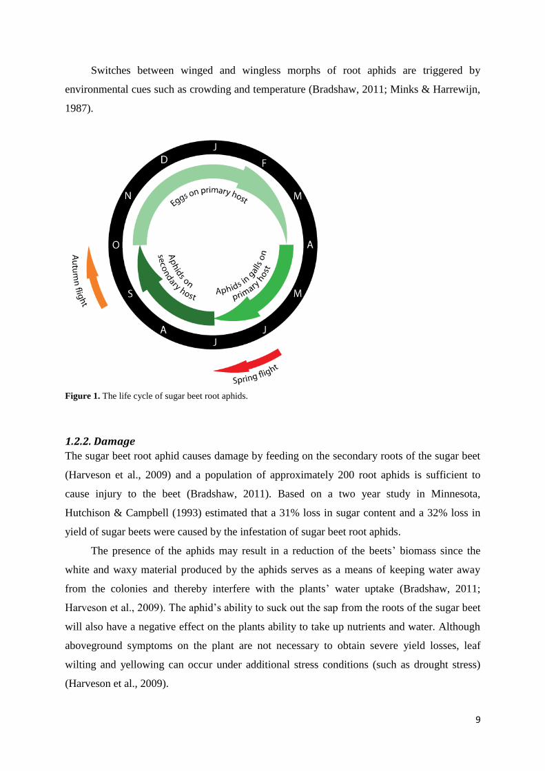
P. betae has a complex life cycle (fig. 1) switching between two types of hosts. In spring

overwintering eggs hatch giving rise to wingless females on the primary host (most

commonly narrowleaf cottonwood (Populus angustifolia), but also black cottonwood

(Populus trichocarpa) and balsam poplar (Populus balsamifera)). The wingless females

initiate galls on the leaves of the primary host in which winged females (the spring forms)

with a black head and thorax and a green abdomen are produced asexually (Bradshaw, 2011;

Harper & Whitfield, 2001; Harveson et al., 2009; Moran & Whitham, 1988).

In early summer the winged females migrate to the secondary host consisting of sugar

beet (Beta vulgaris L.) and various weeds, such as species of Rumex, Chenopodium and

Polygonum. Underground at the roots of the secondary host, several generations of yellowish

white and broadly oval wingless female aphids (the summer forms) are produced asexually.

Since the summer forms of sugar beet root aphids secrete a white waxy material the colonies

often appear “moldy” (Bradshaw, 2011; Harveson et al., 2009; Moran & Whitham, 1988;

Moran & Whitham, 1990).

In autumn both winged and wingless aphids (the fall forms) are produced and just as the

spring forms, these aphids have a black head and thorax and a green abdomen. Winged aphids

fly back to the primary host, while the wingless aphids stay and overwinter in the soil of the

secondary host. On the primary host several wingless female and male aphids are produced in

protected places on the bark. Then in a crevice in the bark or under the bark of dead branches

eggs are deposited after mating and are left to overwinter (Bradshaw, 2011; Harper &

Whitfield, 2001; Moran & Whitham, 1988).

9

Switches between winged and wingless morphs of root aphids are triggered by

environmental cues such as crowding and temperature (Bradshaw, 2011; Minks & Harrewijn,

1987).

Figure 1. The life cycle of sugar beet root aphids.

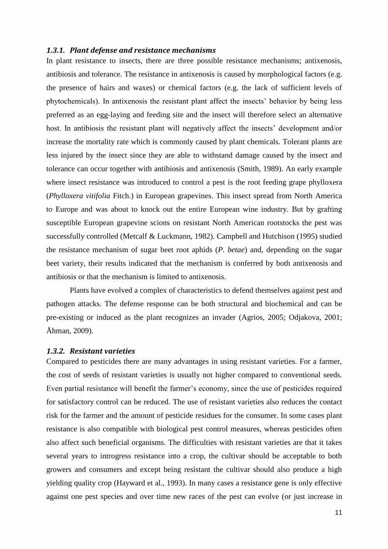
1.2.2. Damage

The sugar beet root aphid causes damage by feeding on the secondary roots of the sugar beet

(Harveson et al., 2009) and a population of approximately 200 root aphids is sufficient to

cause injury to the beet (Bradshaw, 2011). Based on a two year study in Minnesota,

Hutchison & Campbell (1993) estimated that a 31% loss in sugar content and a 32% loss in

yield of sugar beets were caused by the infestation of sugar beet root aphids.

The presence of the aphids may result in a reduction of the beets’ biomass since the

white and waxy material produced by the aphids serves as a means of keeping water away

from the colonies and thereby interfere with the plants’ water uptake (Bradshaw, 2011;

Harveson et al., 2009). The aphid’s ability to suck out the sap from the roots of the sugar beet

will also have a negative effect on the plants ability to take up nutrients and water. Although

aboveground symptoms on the plant are not necessary to obtain severe yield losses, leaf

wilting and yellowing can occur under additional stress conditions (such as drought stress)

(Harveson et al., 2009).

10

The infestation dynamics is most likely a result from a combination of different factors,

such as the abundance of wingless adults late in the season that will remain in the soil in the

fall, the number of severe weather days during the winter (e.g. number of days with

temperatures <-18oC and snow cover <12.7 cm) and dryer conditions during the growing

season (Hutchison & Campbell, 1993).

1.2.3. Management

At present, the use of resistant varieties of sugar beet is the best alternative for managing

sugar beet root aphids. However, there are some other strategies to minimize infestation. One

option is to keep the soil moist, since the impact of aphids increase under drought conditions.

Also the soil type can contribute to the impact of the aphids. A heavier soil may crack which

will provide the aphids with pathways to the roots whereas in a lighter soil cracks are not

likely to develop. On the other hand it will probably comprise better drainage which will keep

moisture away from the aphid colonies. In areas where aphids overwinter in the soil, crop

rotation and good weed control can reduce the infestation risk. There are also some natural

enemies, e.g. the chloropid fly (Thaumatomyia glabra), which feed on aphids in galls and in

the soil (Harveson et al., 2009).

1.3. Resistance Pests and diseases can be a major factor affecting the yield and quality of the cultivated crop

which makes breeding of cultivars genetically resistant an important objective of plant

breeding (Brown & Caligari, 2008). Resistance can be classified as nonhost resistance and

host resistance. Plants with nonhost resistance are simply not a host for the pathogen because

of many plant characteristics that differs from hosts. Host plants with polygenic resistance

activate genes that will have a quantitative resistance effect. Monogenic resistant plants

defend themselves through the presence of matching genes in the host plant and the pathogen.

The host plant contains a few resistance genes (R-genes) per pathogen and likewise the

pathogen carries matching avirulence genes (A-genes) for each R-gene (Agrios, 2005). R-

genes have previously been shown to be involved in aphid resistance, e.g. in tomato,

Pallipparambil et al. (2010) found that the R-gene Mi-1.2 is involved in resistance against

several herbivores including aphids (Macrosiphum euphorbiae).

11

1.3.1. Plant defense and resistance mechanisms

In plant resistance to insects, there are three possible resistance mechanisms; antixenosis,

antibiosis and tolerance. The resistance in antixenosis is caused by morphological factors (e.g.

the presence of hairs and waxes) or chemical factors (e.g. the lack of sufficient levels of

phytochemicals). In antixenosis the resistant plant affect the insects’ behavior by being less

preferred as an egg-laying and feeding site and the insect will therefore select an alternative

host. In antibiosis the resistant plant will negatively affect the insects’ development and/or

increase the mortality rate which is commonly caused by plant chemicals. Tolerant plants are

less injured by the insect since they are able to withstand damage caused by the insect and

tolerance can occur together with antibiosis and antixenosis (Smith, 1989). An early example

where insect resistance was introduced to control a pest is the root feeding grape phylloxera

(Phylloxera vitifolia Fitch.) in European grapevines. This insect spread from North America

to Europe and was about to knock out the entire European wine industry. But by grafting

susceptible European grapevine scions on resistant North American rootstocks the pest was

successfully controlled (Metcalf & Luckmann, 1982). Campbell and Hutchison (1995) studied

the resistance mechanism of sugar beet root aphids (P. betae) and, depending on the sugar

beet variety, their results indicated that the mechanism is conferred by both antixenosis and

antibiosis or that the mechanism is limited to antixenosis.

Plants have evolved a complex of characteristics to defend themselves against pest and

pathogen attacks. The defense response can be both structural and biochemical and can be

pre-existing or induced as the plant recognizes an invader (Agrios, 2005; Odjakova, 2001;

Åhman, 2009).

1.3.2. Resistant varieties

Compared to pesticides there are many advantages in using resistant varieties. For a farmer,

the cost of seeds of resistant varieties is usually not higher compared to conventional seeds.

Even partial resistance will benefit the farmer’s economy, since the use of pesticides required

for satisfactory control can be reduced. The use of resistant varieties also reduces the contact

risk for the farmer and the amount of pesticide residues for the consumer. In some cases plant

resistance is also compatible with biological pest control measures, whereas pesticides often

also affect such beneficial organisms. The difficulties with resistant varieties are that it takes

several years to introgress resistance into a crop, the cultivar should be acceptable to both

growers and consumers and except being resistant the cultivar should also produce a high

yielding quality crop (Hayward et al., 1993). In many cases a resistance gene is only effective

against one pest species and over time new races of the pest can evolve (or just increase in

12

numbers) and thereby overcome the resistance in the host plant which will affect the

durability of the resistance in the cultivar (Brown & Caligari, 2008; Hayward et al., 1993).

1.4. Plant Breeding Ever since Mendel’s work in the middle of the 19

th century, plant breeding has been an

important tool to improve crop characteristics (Brown & Caligari, 2008). With plant breeding

a particular objective is obtained by deliberate selection towards the objective (Hayward et al.,

1993). To recombine variation in traits of use plants are crossed. The produced offspring are

then evaluated and the recombinants displaying the genes of interest are selected and then

used in further crosses (Acquaah, 2007). The most common breeding objectives are to

increase crop yield, improve the end-use quality and to increase pest and disease resistance

(Brown & Caligari, 2008).

In breeding, one can distinguish between qualitative and quantitative genetics. In

qualitative genetics alleles at a single locus or a few loci control the inheritance, while in

quantitative genetics this is controlled by alleles at more loci and the trait is commonly

influenced by the environment. Characters showing quantitative variation are referred to as

polygenic systems since they are mediated by a number of supplementary genes all effecting

the total variation. The relationship between genes and the affected characters is often very

complex as several genes can have the same primary action and likewise a single gene can

have several primary actions (Brown & Caligari, 2008; Hayward et al., 1993).

Examples of qualitative traits are flower color and plant size (dwarf vs. normal) and

quantitative traits are complex traits such as, yield and maturity date. Genes controlling the

variation of complex traits are called polygenes and are present at quantitative trait loci

(QTLs). The difficulties in studying complex traits comes from a range of variation since

many genotypes can show the same phenotype, the true genotype can be obscured by

dominance, the environment can cause variation and the effect of one genotype at one locus

can depend on the genotype at another locus (epistasis) (Hayward et al., 1993).

1.4.1. Sugar beet breeding

With sugar beet breeding one wants to obtain reliable varieties that result in a high yield of

sugar per unit area in relation to the cost of production, and varieties that accord with growers

and sugar factories requirements regarding morphology, anatomy, physiology and chemical

traits of the beet. The root shape is an important morphological character in sugar beet

breeding since it will affect harvesting, storage ability and factory processes. Anatomical

13

characters, such as cell size and number of vascular bundles are significant features which

have an impact on sugar extractability. As for physiological characters premature bolting is an

important breeding objective, particularly in temperate areas and where autumn sowing is

performed, since this character will cause difficulties in harvesting and reduce the yield.

Another important physiological aspect in sugar beet breeding is resistance to pests and

diseases which have a great impact on yield and pesticide inputs. Chemically, sugar beets

should contain higher sucrose content relative to sodium and potassium salts, α-amino-

nitrogen and betaine, since these characters are of great impact in the sugar crystallization

processes (Cooke & Scott, 1993).

In sugar beet, the hybrid breeding method is the breeding method commonly used. To

produce hybrid seeds male sterility is very important and the most important system in hybrid

seed production is cytoplasmic male sterility (CMS) which enables efficient and economic

hybrid seed production (Hayward et al., 1993).

1.5. DNA (deoxyribonucleic acid) markers Genetic markers are tags for genes at certain positions (loci) within the chromosomes that

cause genetic differences between individual organisms or species. This means that the

markers do not necessarily occur at a coding region that affects the phenotype of a trait but

they are located near the gene affecting the trait (Collard et al., 2005).

DNA (deoxyribonucleic acid) markers are the most commonly used genetic marker

nowadays (Collard et al., 2005) and results from different spontaneous mutations at the DNA

level (Paterson, 1996). Since phenotype-based identification of QTLs is not possible (as many

genotypes may display the same phenotype) the development of DNA markers has facilitated

the localization of QTLs and thereby the characterization of quantitative traits (Collard et al.,

2005; Hayward et al., 1993). Genetic variation observed at a DNA marker gives information

about alleles which can be associated to the allelic forms of genes of interests (Hartl & Jones,

2005). DNA markers that display differences between individuals are called polymorphic

markers. On the contrary, DNA markers that do not show any differences between individuals

are called monomorphic markers. Polymorphic markers can be further divided into

codominant and dominant markers. Codominant markers can distinguish homozygotes from

heterozygotes and can represent many different alleles, whereas dominant markers are either

present or absent, thereby unable to make the distinction between homozygotes and

heterozygotes and represent only two alleles (Collard et al., 2005).

14

There is a wide field of application for DNA markers, e.g. they can be used to identify

genes involved in disease resistance and food safety, to create genetic maps, to map simple

traits, QTLs and mutations or to characterize transformants (Birren & Lai, 1996; Hartl &

Jones, 2005). With a linkage map the position and distance between markers at different loci

along the chromosome can be displayed. With an adequate number of markers, and a

population in disequilibrium, the linkage map can be used to locate genes and QTLs that are

associated with a trait of interest and this is referred to as QTL maps. During meiosis genes,

and markers, segregate via chromosome recombination, also called crossing-over, making up

the foundation of a QTL map (Collard et al., 2005; Hartl & Jones, 2005; Lynch & Walsh,

1998). The closer or more tightly-linked the genes or markers are the more likely it is that

they will be transferred together from the parent to the progeny. The order and distance

between markers can be estimated by analyzing markers where a lower frequency of

recombination between two markers indicates that the markers are more closely located in the

chromosome (Hartl & Jones, 2005). To construct a linkage map of a mapping population,

identification of polymorphism and linkage analysis of markers are required. The mapping

population needs to be a segregating plant population and the parents in the population need

to differ in one or more traits (Collard et al., 2005).

1.5.1. Different types of DNA markers

There are different types of DNA markers used in marker analysis; for example the

codominant markers consisting of Restriction Fragment Length Polymorphisms (RFLP)

(Hartl & Jones, 2005; Winter & Kahl, 1995), Simple Sequence Repeats (SSRs) (Hartl &

Jones, 2005; McCouch et al., 1997; Powell et al., 1996; Taramino & Tingey, 1996) and

Single-Nucleotide Polymorphisms (SNPs) (Schneider et al., 2007), and the dominant markers

consisting of Random Amplified Polymorphic DNAs (RAPDs) (Hartl & Jones, 2005; Lynch

& Walsh, 1998; Williams et al., 1990) and Amplified Fragment Length Polymorphisms

(AFLPs) (Vos et al., 1995). Most of these marker systems are time-consuming and expensive,

and for some of them the amounts of polymorphisms are low and the methodology

complicated (Collard et al., 2005; Schulman, 2007; Vos et al., 1995; Winter & Kahl, 1995).

With the development of high-throughput techniques for the detection of SNPs, this type of

DNA-marker has become more advantageous and is today widely used (Landegren et al.,

1998; Schneider et al., 2001).

15

1.5.2. Single-Nucleotide Polymorphism (SNP)

SNPs are the latest generation of DNA markers (Schneider et al., 2007) and constitute the

most frequent type of genetic variation in natural populations of a species (Schneider et al.,

2001). SNPs are distributed uniformly across the genomes and at one SNP locus, only two

alleles and three genotypes among a given population are possible (fig. 2); e.g. homozygous

with either T-A or G-C at the same site at both homologous chromosomes or heterozygous

with T-A in one chromosome and G-C at the same site in the homologous chromosome (Hartl

& Jones, 2005). By DNA sequencing such differences between the alleles at a certain position

can be detected (Schneider et al., 2001).

Functional differences by an SNP are more likely to occur when the SNP is located in a

coding region or in a regulatory region compared to an SNP located elsewhere. Even though

the majority of SNPs does not have an effect on a gene function, many mapped SNPs can be

very useful as markers to find SNPs that affect gene function (Collins et al., 1998). Schneider

et al. (2001) studied the frequency of SNPs and the fraction of polymorphic loci in sugar beet

using EST (Expressed Sequence Tag) sequences. After the sequencing of 37 gene fragments

of sugar beet, the results showed that the frequency of SNPs corresponded to 1 SNP every

130 bp. Most of the SNPs (65%) were located in introns and therefore do not change the gene

product but could still induce a phenotypic effect since they might affect the transcription rate

or stability of the mRNA.

There are some advantages of using SNPs as markers in genetic analysis; SNPs located

in genes might affect protein structure or expression levels and compared to SSRs SNPs are

more common in the genome, easier to score and more stable (Landegren et al., 1998;

Schneider et al., 2001).

Figure 2. Three possible genotypes of an SNP. A and B homozygous, and C heterozygous.

16

1.5.3. Marker-assisted breeding

DNA markers are essential to perform marker-assisted selection (MAS) and facilitate the

mapping and tagging of agriculturally important genes. The use of molecular techniques has

enabled a more rapid transfer of desirable genes between different varieties, the introgression

of novel genes from wild species and simplified analysis of polygenic characters (Mohan et

al., 1997; Winter & Kahl, 1995).

Prior to the discovery of DNA markers, a resistant donor line was crossed with an

agronomically better cultivar to conduct single gene introgression. After repeated testings,

selfings and backcrossings the cultivar mainly contained the gene of interest from the donor

genome. This process can be speeded up by several plant generations if DNA markers are

used to select the offspring containing the lowest amount of the donor genome in every

generation (Winter & Kahl, 1995) and many rounds of selection can be performed during a

year (Mohan et al., 1997). MAS contributes more advantages in breeding for disease

resistance; unreliable results due to poor inoculation methods are avoided since selection can

be achieved without inoculation and breeding can be carried out in areas where safety

regulations do not allow field inoculation with the pathogen (Hayward et al., 1993).

At Syngenta, SNPs are the only DNA markers used in MAS of sugar beet. Every year

approximately 200 000 plants are analyzed resulting in approximately 2 million datapoints

and these numbers are constantly increasing. The most important traits that are subjected to

MAS are resistance to diseases (such as rhizomania and cercospora), nematodes and bolting

and more complex traits (such as sugar yield). Most of the marker analyses are done on F2

plants so that only the most favorable genotypes will be selfed for line production. This can

be regarded as a pre-selection, so for example if marker selection is done in the F2 for a

single-locus resistance, only the 25% of the plants that are homozygous for the resistance

allele will be selfed. Compared to a random inbreeding, this will save a lot of resources

(inbreeding, phenotyping) that would have otherwise been spent on genotypes that are either

segregating or susceptible at the resistance locus. Marker selection is also used in back-

crossing programs, something that has increased after the introduction of genetically modified

(GM) sugar beets in the USA and Canada. In some materials, markers are also used to modify

many traits at the same time with the aim of creating superior lines. QTL analysis is done in

large mapping populations and based on the results the ideal genotype coming from that cross

can be described. In subsequent generations of the same cross, markers are used to create

genotypes that are close to this ideal genotype and can then afterwards be tested in the field

(Kraft, T., personal communication, 2011).

17

To increase the precision at selection it is necessary to fine map the locus. For this, a

large mapping population, usually consisting of thousands of individuals and segregating for a

trait of interest, needs to be developed. Using flanking markers, individuals showing

recombination events within this locus are selected and selfed in order to get fixed

recombinant lines in the next generation. The next step is to enrich the region with new

markers (when sequences are available). Based on the phenotype and the new genotype of

each fixed recombinant line a new genetic interval can be defined (Pin, P., personal

communication, 2011).

1.6. Sequencing With DNA sequencing the order of the nucleotide bases in the DNA molecule are determined

(Miyamoto & Cracraft, 1991). During the 1970s, two different types of DNA sequencing

methods were developed; the chemical sequencing, and the chain termination method (Kim et

al., 2008). The chemical sequencing method is based on base-specific chemical reactions to

determine the bases in the DNA sequence (Maxam & Gilbert, 1977; Miyamoto & Cracraft,

1991), and the chain-terminator method uses radioactively or fluorescently labeled ddNTPs

(dideoxy nucleoside triphosphates) which facilitates detection in automated sequencing

machines (Kim et al, 2008; Sanger, 1980). Compared to the chemical sequencing method, the

chain-terminator method is more commonly used since it is more amenable to automation and

needs fewer toxic chemicals and lower amounts of radioisotopes (Manz et al., 2004;

Miyamoto & Cracraft, 1991; Schuster, 2008).

To increase the throughput and lower the cost of DNA sequencing several next-

generation sequencing (NGS) technologies have been developed (Metzker, 2010; Schuster,

2008). One of them, the 454 technology, uses a sequencing by synthesis approach. During the

sequencing process light are generated as nucleotides complementary to the template strand

are incorporated (454 Life Sciences). Illumina sequencing (previously known as Solexa) is

another NGS method supporting parallel sequencing (Illumina, 2011a). Based on reversible

terminators, single nucleotides can be detected when they are incorporated into the DNA

strand. Nucleotides added to the DNA during the sequencing are fluorescently labeled, hence

enabling identification (Illumina, 2011b). At a lower cost (in comparison with the chemical

sequencing and the chain terminator method), millions of sequence reads can be generated in

a single run of NGS (Metzker, 2010), thereby opening up for new areas of applications. For

instance, the sequencing of entire genomes of hundreds of new organisms became possible.

18

NGS can also be applied for the re-sequencing of known genomes and the characterization of

whole transcription profiles.

1.7. Aim Prior to this study, Syngenta had mapped a single locus controlling the sugar beet root aphid

resistance to an interval of ±10 cM (centimorgan) at chromosome I in sugar beet. Based on a

field test in USA with 225 recombinant F3 lines and a molecular analysis with two flanking

SNP markers (SS0011 and SS0014) several sugar beet lines showed crossing-over in that

interval, but since no polymorphic markers were found or could be developed within the

genetic interval, it has not been possible to narrow down the region. With the ongoing

sequencing of the whole sugar beet genome, it is now possible to look for new

polymorphisms at sequences located between the two previous markers and to saturate the

locus with new markers.

The core objective of this master thesis was to initiate a fine mapping of the sugar beet

root aphid resistance locus (from now on referred to as SBRA resistance locus) by:

(i) Implementing a robust phenotypic greenhouse test for the SBRA resistance.

(ii) Developing new SNP markers closely linked to the SBRA resistance locus.

Primers were designed to amplify fragments of scaffolds flanking the SBRA resistance locus

of both resistant and susceptible lines. The sequences of the amplified products were

compared to identify polymorphisms which could be used to develop more precise SNP

markers.

(iii) Combining the phenotypic data with the genotypic data to fine map the

resistance locus.

19

2. Materials and Methods

2.1. Plant material To create the mapping population of 225 recombinant lines, Syngenta has crossed a resistant

parent (LGV128) with a susceptible parent (L327). All plants from the F2 population from

that cross were selfed, and one plant from each offspring seed lot (F3 level) was selected and

selfed again. The genotyping was done on the selected F3 plants and phenotyping on the

offspring from these plants (F4 lines).

2.1.1. Phenotypic test

For the phenotypic test, six replicates (plants) of 40 different lines were used, out of which:

i) Thirty recombinant lines were selected from the 62 recombinant lines used in the

marker analysis. The selection was based on the access to seeds. The 62 lines were

in turn selected from the mapping population of 225 recombinant lines.

ii) Five F4 lines (JL9100, JL9400, JL94XXa, JL94XXb and JL9500) were derived

from a cross between the resistant parent (LGV128) and another susceptible parent

(L397).

iii) One F4 line (JL8Y00) was derived from a cross between the resistant parent

(LGV128) and another susceptible parent (L408).

iv) One line was the resistant parent (LGV128) and two other known resistant lines

(KK0300 and IA3J00) were also included.

v) One line was a control known as resistant.

2.1.2. Marker analysis

The plant material for the marker analysis consisted in total of 94 bulked DNA samples, out

of which:

i) Sixtytwo samples were recombinant lines selected from the mapping population

of 225 lines. The 62 lines were selected due to the fact that they showed

crossing-over in the interval for the SBRA resistance locus.

ii) Three samples were derived from three F3 lines (JL9100, JL9400, JL9500)

generated by a cross between the resistant parent (LGV128) and another

susceptible parent (L397)

iii) One sample were derived from one F3 line (JL8Y00) generated by a cross

between the resistant parent (LGV128) and yet another susceptible line (L408).

20

iv) Four samples were the resistant parent (LGV128) and the three susceptible

parents (L327, L397 and L408).

v) Two samples were other known resistant lines (KK0300 and IA3J00).

vi) Fifteen and seven samples were other known susceptible and resistant lines

respectively.

For all lines, except four, genomic DNA was already extracted and ready to use.

2.2. Insect material For the phenotypic test, sugar beet root aphids (Pemphigus betae) were kindly provided by

PhD Jeff Bradshaw at the University of Nebraska-Lincoln, USA.

2.3. Phenotypic test The sugar beet root aphids were kept on the roots of potted sugar beet plants (in which they

were shipped oversea from USA) in a climate chamber in the quarantine laboratory. With a

brush, the aphids were transferred to new sugar beet plants for reproduction (appendix II, fig.

1). To avoid the development of winged aphids the plants were kept at 12oC.

The test was performed with various resistant and susceptible elite lines, as well as the

recombinant lines for the SBRA resistance locus. For each line, 6 individual plants

(replicates) were tested. One week after sowing the plants were transferred to bigger pots and

then after another two weeks two cells (wholes), approximately 8 cm deep and 1.5 cm in

diameter, were made into the soil of each pot and sealed with corks (appendix II, fig. 2). The

plants were left for two weeks so that the roots would grow into the cells. Then the plants

were moved to tents in a climate chamber (22oC/20

oC (D/N)) and by the use of a brush each

cell was infected with five sugar beet root aphids (in total ten aphids per plant). To avoid too

high water levels in the soil (and consequently minimizing the risk that the aphids would

drown) but still keep the soil moist, a blanket was placed at the bottom of the tent to facilitate

watering from the bottom of the pot.

Three weeks after infection each inoculated plant was scored individually on a scale of

1-9 (appendix III, fig. 1), where 1 is susceptible and 9 is resistant. The results were then used

to estimate a mean value for each line representing the phenotype of that line.

21

2.4. DNA isolation Fresh leaf samples were harvested from young sugar beet plants and placed in wells of a 96-

well box. The tissues were grinded into a fine powder using glass beads. Genomic DNA was

isolated according to the DNA KAc (potassium acetate) isolation method and started by

adding 250 µl of extraction buffer consisting of 100 mM tris-HCL, 1 M NaCl (sodium

chloride), 10 mM EDTA (ethylenediaminetetraacetic acid) and 1% SDS (sodium dodecyl

sulfate), pH 8.0 to each sample. The box was shaken gently and placed at 65oC for 90

minutes. After incubation, the box was cooled down on ice for 5 minutes and then

centrifuged. To each well, 150 µl of cold 5 M KAc were added and mixed. After 30-60

minutes of incubation on ice, the box was centrifuged for 10 minutes at 3800 rpm. For the

precipitation of the DNA, 40 µl of the upper phase were transferred to a new 96-well box

containing 100 µl of isopropanol (2-propanol). The box was inverted several times to help the

precipitation and centrifuged for 20 minutes at 3800 rpm. The isopropanol was discarded by

inverting the box and 200 µl of 70% EtOH (ethanol) were added to clean the pellet of DNA.

After 10 minutes of centrifugation at 3800 rpm, EtOH was discarded by inverting the box and

the pellets air dried. 400 µl TE 1x buffer (Tris-EDTA buffer) were added to resuspend the

pellets. The box was shaken on a vortex and incubated at 65oC for 10 minutes to aid the

resuspension. DNA solutions were stored at -20oC.

2.5. In silico selection of DNA targets The recent sequencing of the whole sugar beet genome generated nearly 740 Mb (unpublished

data). Hundreds of thousands of scaffolds were loaded into a sequence database. Using

previous marker information, it has been possible to anchor thousands of scaffolds to the

sugar beet genetic map. In this study, 6 scaffolds were identified in the vicinity of markers

SS0011 and SS0014. All together, the 6 scaffolds consist of 4.4 Mb which overlap partially.

However, a single superscaffold could not be assembled from the 6 scaffolds, which

unfortunately resulted in a gap in the middle of the locus. From the sequences, 32 primer

pairs, spread all over the locus, were designed using Primer Express program (Applied

Biosystems, Inc, USA).

2.6. Polymerase chain reaction (PCR) PCR were performed in 96-well plates using the 32 primer pairs specifically designed for the

6 scaffold sequences that were identified in close proximity to the SBRA resistance locus in

22

the in silico search. The PCR mix was as follows: 2.968 µl ddH2O, 1 µl [2.5 mM] dNTP mix

(deoxyribonucleotide triphosphate), 1 µl [10x] AmpliTaq Gold® buffer, 0.8 µl [25 mM]

MgCl2 (Magnesium chloride), 0.066 µl [50 µM] forward primer, 0.066 µl [50 µM] reverse

primer and 0.1 µl [5 U/µl] AmpliTaq Gold® (Applied Biosystems, Inc, USA). As template 4

µl of DNA was added to the PCR mix. After a quick centrifugation, the PCR was performed

according to the program in table 1 for all 32 primer pairs using a GeneAmp® PCR System

9700 (Applied Biosystems, Inc, USA).

Table 1. PCR program for amplification of DNA on a GeneAmp® PCR System 9700 (Applied Biosystems, Inc,

USA).

Cycle Temperature (oC) Time (min.)

1 95 10:00

35

94 0:30

60 0:30

72 0:30

1 72 5:00

1 4 ∞

2.7. Control of the PCR products Prior to sequencing, approximately 8 µl of the PCR products were loaded on a 2% agarose gel

to ensure that the amplification resulted in a single and specific product. Agarose gel was

prepared using TAE 1x buffer (tris-acetate-EDTA). Ethidium bromide was added in the gel.

After polymerization of the agarose gel, loading buffer was added to the PCR product and the

mix was loaded onto the gel. The electrophoresis was performed under 200 V for 30-45

minutes. After electrophoresis, the PCR products were visualized under UV light. By the use

of a ladder the sizes of the obtained bands were estimated and then compared to the expected

sizes of the products (appendix I, fig. 1).

2.8. Sequencing and SNP discovery

After the PCR, 2 µl of each PCR product were transferred to a new 96-well plate. To each

well, 5 µl [0.5 µM] of sequencing primer (in this case the forward primer that were used in

the PCR) was added. The sequencing plates were sent for sequencing to the Syngenta

sequencing facility at SBI, North Carolina, USA. The raw sequencing data were assembled

using SeqMan (DNASTAR, Inc, USA). Alignments were manually adjusted and sequencing

artifacts were corrected. Polymorphisms were then extracted from the SeqMan file and

exported to Excel where the sugar beet lines were grouped based on their alleles.

23

3. Results

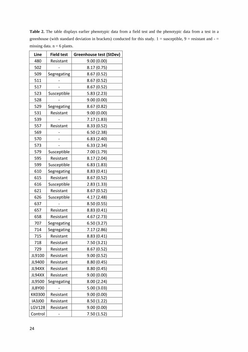
3.1. Phenotypic test

Many of the lines scored fairly consistent, e.g. the resistant parent LGV128, and the resistant

line KK0300 scored 9 on all six replicates. Other lines, e.g. line 707 and line 718, displayed a

more varying degree of infection (as seen by the large standard deviations), ranging between a

score of 1-9 within the same line (table 2).

In comparison with earlier phenotypic data from a field test (table 2); many of the lines

showing resistance in the field test also scored a high value in the greenhouse test, many of

the susceptible lines scored a low value in the greenhouse test and many of the segregating

lines showed a varying score in the greenhouse test. However, some lines displayed

inconsistent data when comparing the earlier phenotypic data with the new phenotypic data.

For example, line 579 scored 7.00 in the greenhouse test (table 2), but showed susceptibility

in the previous field test, which could be a result from escapes (plants where the inoculation

were unsuccessful) in the greenhouse test.

24

Table 2. The table displays earlier phenotypic data from a field test and the phenotypic data from a test in a

greenhouse (with standard deviation in brackets) conducted for this study. 1 = susceptible, 9 = resistant and - =

missing data. n = 6 plants.

Line Field test Greenhouse test (StDev)

480 Resistant 9.00 (0.00)

502 - 8.17 (0.75)

509 Segregating 8.67 (0.52)

511 - 8.67 (0.52)

517 - 8.67 (0.52)

523 Susceptible 5.83 (2.23)

528 - 9.00 (0.00)


531 Resistant 9.00 (0.00)

539 - 7.17 (1.83)

557 Resistant 8.33 (0.52)

569 - 6.50 (2.38)

570 - 6.83 (2.40)

573 - 6.33 (2.34)


595 Resistant 8.17 (2.04)



615 Resistant 8.67 (0.52)


621 Resistant 8.67 (0.52)


637 - 8.50 (0.55)

657 Resistant 8.83 (0.41)

658 Resistant 4.67 (2.73)



715 Resistant 8.83 (0.41)

718 Resistant 7.50 (3.21)

729 Resistant 8.67 (0.52)

JL9100 Resistant 9.00 (0.52)

JL9400 Resistant 8.80 (0.45)

JL94XX Resistant 8.80 (0.45)

JL94XX Resistant 9.00 (0.00)

JL9500 Segregating 8.00 (2.24)

JL8Y00 - 5.00 (3.03)

KK0300 Resistant 9.00 (0.00)

IA3J00 Resistant 8.50 (1.22)

LGV128 Resistant 9.00 (0.00)

Control - 7.50 (1.52)

25

3.2. Target selection Totally, 5 scaffolds were identified from the in silico search in the SS0011-SS0014 genetic

window (fig. 3). Unfortunately not all of the scaffolds overlap with each other which results

into 3 gaps; one between the adjacent scaffold A and superscaffold BC, a second between the

two superscaffolds BC and DE, and a third between superscaffold DE and scaffold F.

Figure 3. The figure shows the order of the scaffolds (A-F). The numbers 18 and 23 are genetic positions in cM

on the genetic reference map. 39PG03, MS0654, SS0011 and SS0014 represent the positions of markers

previously developed and mapped in the vicinity of the SBRA resistance locus.

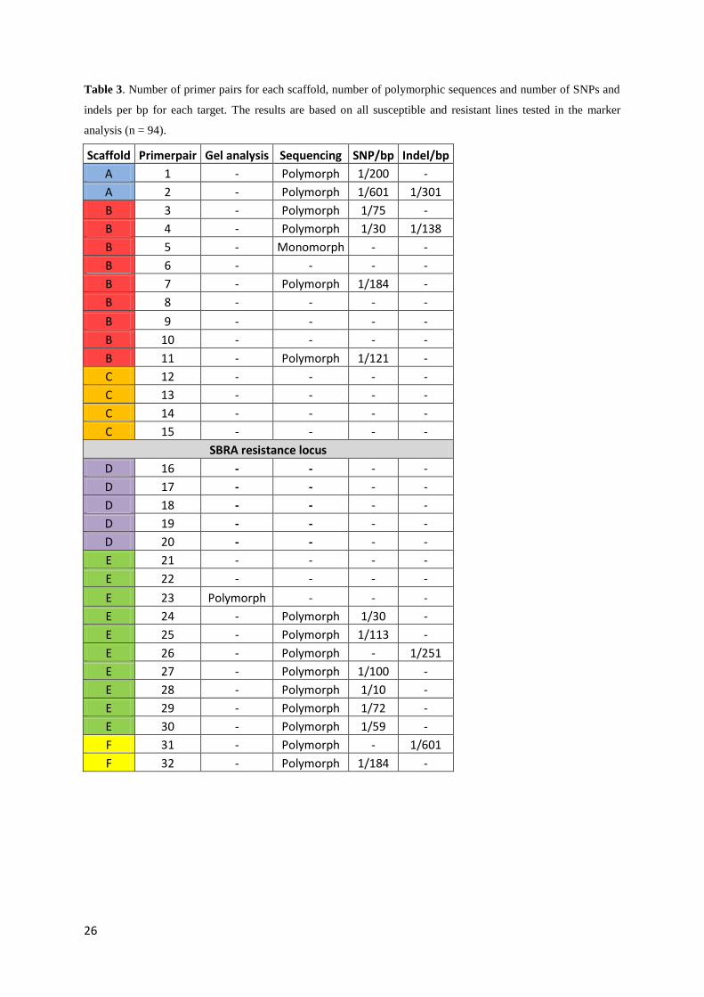
3.3. Sequencing As illustrated in table 3, 32 primer pairs were used to amplify and sequence target fragments

of the 6 scaffolds in the vicinity of the SBRA resistance locus. Out of these 32 targets and

based on all 94 genotyped lines, 16 targets were polymorphic (out of which one was analyzed

on a gel), 1 target was monomorphic and 15 targets failed. On average (in the successfully

sequenced targets), 1 SNP occurred every 137 bp and 1 indel occurred every 323 bp. For

some of the targets where the sequencing failed, the PCR products were tested on a gel. All of

the tested products showed very weak bands or no bands at all, indicating that the targets had

not been amplified.

26

Table 3. Number of primer pairs for each scaffold, number of polymorphic sequences and number of SNPs and

indels per bp for each target. The results are based on all susceptible and resistant lines tested in the marker

analysis (n = 94).

Scaffold Primerpair Gel analysis Sequencing SNP/bp Indel/bp

A 1 - Polymorph 1/200 -

A 2 - Polymorph 1/601 1/301

B 3 - Polymorph 1/75 -

B 4 - Polymorph 1/30 1/138

B 5 - Monomorph - -

B 6 - - - -


B 8 - - - -

B 9 - - - -

B 10 - - - -


C 12 - - - -

C 13 - - - -

C 14 - - - -

C 15 - - - -

SBRA resistance locus

D 16 - - - -

D 17 - - - -

D 18 - - - -

D 19 - - - -

D 20 - - - -

E 21 - - - -

E 22 - - - -

E 23 Polymorph - - -

E 24 - Polymorph 1/30 -


E 26 - Polymorph - 1/251





F 31 - Polymorph - 1/601

F 32 - Polymorph 1/184 -

27

For the mapping population five new SNP markers have been identified, other

polymorphic markers either did not show polymorphism in the mapping population or

displayed the same information as another marker. Two of the five SNP markers (E25 and

E29) are located in the genetic window between markers SS0011 and SS0014 (fig. 4). The

markers found has also ensured that the order of the scaffolds are as in figure 4; scaffold A

being furthest away from the locus and superscaffolds BC and DE being closest to the locus.

Figure 4. The figure shows the best markers (A1, B7, E25, E29 and F31) found in scaffolds A-F. The figure is

based on the 30 lines that were phenotypically tested in the greenhouse (except for seven lines that showed

inconsistent data) and in addition two other lines that could not be phenotyped due to lack of seeds. 39PG03,

MS0654, SS0011 and SS0014 represent the positions of markers previously developed and mapped in the

vicinity of the SBRA resistance locus. Numbers 18 and 23 are genetic positions in cM on the genetic reference

map. X indicates the number of lines showing cross-overs between the markers.

3.4. Fine Mapping The fine mapping of a locus can be illustrated by a graphical map which is based on

genotypic information of different markers and phenotypic data of each line. Tables 4 and 5

illustrate how a graphical map is constructed based on that information. The top row of the

tables denotes the various markers, except the one named SBRA which represents the

phenotype of each individual line. In the left column the various lines are listed. For each line,

“S”, “R” and “H” represents the genotype for each marker, where “S” is homozygous for the

susceptible allele, “R” is homozygous for the resistant allele and “H” is segregating

(heterozygous). Numbers “1”, “1/2” and “2” denotes the alleles (genotypes) for each new

marker that is being mapped.

28

Table 4. A part of the graphical map before this study started.

39PG03 SBRA MS0654

499 H H R

509 R H H

523 S S H

729 H R R

579 S S H

595 S R R

616 H S S

Table 5a. The first polymorphic marker (A1) was added in the column to the right. To see where in the map it fit

in, marker A1 was manually moved around between the markers.

39PG03 SBRA MS0654 A1

499 H H R 1/2

509 R H H 1

523 S S H 2

729 H R R 1/2

579 S S H 2

595 S R R 2

616 H S S 1/2

Table 5b. This table shows why marker A1 does not map between the SBRA resistance locus and the MS0654

marker. For example if marker A1 is placed at this position, flanking markers in line 616 indicates that allele 1/2

should be “S”. However, since allele 1/2 is heterozygous at least one of the flanking markers should be “H”. This

means that marker A1 does not map between the resistance locus and the MS0654 marker.

39PG03 SBRA A1 MS0654

499 H H 1/2 R

509 R H 1 H

523 S S 2 H

729 H R 1/2 R

579 S S 2 H

595 S R 2 R

616 H S 1/2 S

29

Table 5c. By moving marker A1 between marker 39PG03 and the SBRA resistance locus, the profile of the

genotypes match for all individuals, where allele 1 corresponds to genotype “R” and allele 2 to genotype “S”.

This suggests that the marker A1 maps between the 39PG03 marker and the RA locus.

39PG03 A1 SBRA MS0654

499 H 1/2 H R

509 R 1 H H

523 S 2 S H

729 H 1/2 R R

579 S 2 S H

595 S 2 R R

616 H 1/2 S S

Table 5d. The last step is to convert the allele number of marker A1 to the correct genotype: hence, allele 1 is

the resistant genotype, allele 1/2 is the segregating genotype and allele 2 is the susceptible genotype. Following

the same procedure, other markers can be placed in the graphical map.

39PG03 A1 SBRA MS0654

499 H H H R

509 R R H H

523 S S S H

729 H H R R

579 S S S H

595 S S R R

616 H H S S

From the genotypic information of the 5 new SNP markers (A1, B7, E25, E29 and F31)

and the phenotypic data from an earlier field test a graphical map was constructed to illustrate

the fine mapping of the SBRA resistance locus (table 6). With markers B7 and E25 the SBRA

resistance locus has been possible to narrow down. Between the two markers there are 7

recombinant lines (lines 610, 511, 729, 523, 539, 637 and 626), corresponding to a

recombination frequency of 1.6%. Since the phenotypic data of three of the recombinant lines

(lines 511, 539 and 637) (table 6) are uncertain it was not possible to make an exact

estimation of the recombination frequency between a single marker and the resistance locus.

This means that if marker-assisted selection is to be performed using either marker B7 or E25

a recombination frequency varying between 1.1% and 0.4% is expected between the marker

and the resistance gene.

For some of the lines, e.g. line 658 (table 6), the data were inconsistent, which is most

likely due to inaccurate phenotypic data. Line 658 displayed resistance in an earlier field test

30

but scored a low value in the phenotypic test conducted in this study. Since flanking markers

(B7 and E25) of the resistance locus in line 658 are heterozygous, this line is most likely

heterozygous for the SBRA resistance locus.

31

Table 6. Fine mapping of the SBRA resistance locus based on the 30 lines that were phenotypically tested in the

greenhouse (except for six lines that showed inconsistent data) and in addition two other lines that could not be

phenotyped due to lack of seeds. The lines tested are listed in the left column. The top row shows the two

markers (39PG03 and MS0654) previously mapped near the resistance locus and the five new SNP markers (A1,

B7, E25, E29 and F31). The column named SBRA displays the phenotype of each line obtained from a field test

and, in brackets, the phenotypic value from the greenhouse test. “R”: homozygous for the resistant allele, “S”:

homozygous for the susceptible allele and “H”: heterozygous (segregating). The white regions represent

uncertain data.

39PG03 A1 B7 SBRA E25 E29 F31 MS0654

715 R R R R (8.83) R R H H

517 R R R (8.67) R H H H

509 R R H H (8.67) H H H H

529 R R H H (8.67) H H H H

499 H H H H H R R R

610 H H H H (8.83) R - R R

511 H H H (8.67) R R R R

729 H H H R (8.67) R R R R

531 H H R R (9.00) R R R R

621 H H R R (8.67) R - R R

657 H H R R (8.87) R R R R

595 S S R R (8.17) R R R R

528 S S H (9.00) H H H H

523 S S S S (5.23) H H H H

539 S S S (7.17) H H H H

637 S S S (8.50) H H H H

502 S S S (8.17) S R R R

579 S S S S (7.00) S H H H

583 S S S S S H H H

599 S S S S (6.83) S H H H

569 H H S (6.50) S S S S

570 H H S (6.83) S S S S

573 H H S (6.33) S S S S

616 H H S S (2.83) S S S S

626 H H H S (4.17) S S S S

658 H R H R (4.67) H H H R

32

4. Discussion

4.1. Phenotypic test

At Syngenta in Landskrona, this was the first attempt to conduct a phenotypic test to evaluate

root aphid resistance in sugar beet under greenhouse conditions. Overall the phenotypic test

showed to be successful as the results were similar to the results from an earlier field test, but

as expected with a pilot test, there were some difficulties along the way. One problem that

arose was that the soil collapsed in many of the cells after the cells were made. This was most

likely due to the type of soil selected for the test which resulted in different cell depths and

this might have influenced the result. To improve this issue different soil types or mixtures

should be evaluated to find a more firm soil for future phenotypic tests. Another problem with

the phenotypic test was that the development of roots in the cells was very uneven with some

plants showing many roots in the cells and others showing very little or no roots. This is likely

a consequence from uneven watering, making some pots constantly moist and thereby

slowing down the development of the roots. The lack of roots in the cells may have

influenced the survival of the aphids and thus indirectly the amount of escapes. As in other

studies of root aphids where escapes has occurred (Campbell & Hutchison, 1995), the amount

of escapes is a likely reason for some lines (e.g. line 718; table 2), displaying a varying degree

of infection.

Despite those difficulties, the results from the greenhouse phenotypic test mainly

confirmed the phenotype of field tested lines, as most lines that were expected to be resistant

in the phenotypic test showed resistance and most lines that were expected to be susceptible

were susceptible. The new phenotypic data were therefore helpful in evaluating the markers

and fine mapping the SBRA resistance locus.

4.2. Sequencing

The sequencing of segments showed many polymorphisms for many of the scaffolds. On

average, 1 SNP occurred every 137 bp, which is in accordance with the findings of Schneider

et al. (2001) who found 1 SNP every 130 bp in sequenced gene fragments of sugar beet. In

rice SNPs occurred more frequent than indels, suggesting that the use of SNPs are a better

choice when fine mapping the rice blast resistance locus (Hayashi et al. 2004). This also

seems to be the case for the fine mapping of the SBRA resistance locus, since 1 indel

occurred every 323 bp.

33

Closer to the resistance locus the sequencing failed due to lack of amplified PCR

product. This means that it was not possible to evaluate the two scaffolds closest to the

resistance locus (scaffold C and D). The reason for the failed amplification can be due to

technical reasons or that amplification of segments closer to the SBRA resistance locus is

more difficult because of greater re-arrangements near the resistance locus.

4.3. Fine mapping

DNA markers have been used for fine mapping resistance to insects in various plants; e.g.

Kim et al. (2010) used SNPs to fine map the soybean aphid (Aphis glycines Matsumura)

resistance. As illustrated by that study, there are three pre-requirements that are essential to

carry out fine mapping of a resistance locus: (i) a mapping population segregating for a trait

of interest, (ii) molecular markers located in the vicinity of the locus involved in the trait, and

(iii) a robust phenotypic method to test the trait across the population. All of these three pre-

requirements are fulfilled in this project. Important to point out is that in QTL analysis a

polymorphic marker found to be linked to a specific trait in one population is not necessarily

applicable for another population since each population have specific parents (Collard et al.,

2005). This means that when fine mapping the SBRA resistance locus not all polymorphic

markers shown in table 3 could be used for the mapping population (that was used to map the

SBRA resistance to a single locus located at chromosome I). On the contrary, it is not certain

that the five markers that were found useful for the mapping population (table 6) are

applicable when fine mapping the locus in other populations. Since the fine mapping (table 6)

is based on data from the mapping population the discussion will focus on these results. As

previously mentioned, the mapping population consisted of 225 lines which correspond to

450 chromosomes. The DNA markers that were identified in the vicinity of the resistance

locus could, together with the phenotypic data, be used to fine map the SBRA resistance locus

and thereby it was possible to calculate the recombination frequency as an estimation of the

distance between the markers.

In the mapping population 25 recombinant events were found between the two

originally closest polymorphic markers (39PG03 and MS0654) (fig. 4; line 658 is excluded

due to inconsistent data) corresponding to a recombination frequency of 5.6%. Using new

SNP markers identified on scaffold sequences in this study, a new recombination frequency of

1.6% could be estimated between the closest markers B7 and E25. When using two markers

to select plants, plants that are homozygous resistant at both markers will be selected. If

selected plants are not resistant this means that there is a double cross-over between the two

34

markers. The smaller the distance is between the two markers, the more unlikely it is that

there will be a double cross-over between the two markers. If markers B7 and E25 are used as

selection markers, the probability that selected plants will not be homozygous resistant is very

low because the interval between the markers is very small (a recombination frequency of

1.6%) and therefore it is unlikely that there will be a double cross-over between the two

markers. This also means that if only one of the markers is used in marker-assisted selection

the probability of selecting a plant that is not homozygous resistant at the resistance locus is

low, also due to the small interval between the marker and the resistance locus (a

recombination frequency between 1.1% and 0.4%). From this it is possible to conclude that

whether both or only one of markers B7 and E25 are used as selection markers for the root

aphid resistance the probability of selecting plants carrying the resistance will be high and

hence, both markers are useful in marker-assisted breeding for the SBRA resistance.

However, since there are some recombinant lines between markers B7 and E25, there is

still a possibility for the fine mapping to become even more accurate and it might even be

possible to find a marker located in the resistance gene itself. As pointed out by Kim et al.

(2010) the identification of markers closely linked to the resistance locus are valuable in MAS

for the resistance gene. For the fine mapping of the SBRA resistance locus to become more

accurate, the next step will be to sequence new fragments of the superscaffolds BC and DE

(fig. 4) to find new SNPs that are more closely linked to the locus. Moreover, with the

ongoing sequencing of the whole genome of sugar beet, the gap between super scaffolds BC

and DE might be filled in the future and thus enable the sequencing of currently unknown

segments to find polymorphisms that can be used for further marker development. As

phenotypic data are essential in the evaluation of DNA markers, the next step will also be to

conduct a new phenotypic test to get more reliable data that can be used in the fine mapping

of the resistance locus. By improving the test further to avoid the difficulties that arose in the

pilot test, fewer escapes are likely to occur resulting in more reliable data and thereby making

future marker analysis easier.

35

5. Conclusions Prior to this study, a single locus for resistance against sugar beet root aphids was mapped to

chromosome I to an interval with a recombination frequency of 5.6%. The core objective of

this study was to fine map the locus by developing new SNP markers and by developing a

greenhouse phenotypic test that could be used in the evaluation of the markers. The objective

was successfully fulfilled as a phenotypic test was developed under greenhouse conditions

and, although it showed somewhat varying results, it was accurate enough to confirm the

position of the new SNP markers. The study also resulted in five new SNP markers, two of

them being mapped in the genetic window of the two SNP markers found prior to this study.

This made it possible to fine map the SBRA resistance locus and narrowing-down the locus to

a recombination frequency of 1.6% using the two new best SNP markers in the selection,

making the probability of selecting plants that carry the resistance high.

In a short term perspective, the new SNP markers can be used for marker-assisted

selection, knowing that a very small proportion of the selected plants may be heterozygous for

the resistance locus. In a long term perspective, sequencing of new segments of the scaffolds

closest to the locus is necessary to enrich the interval with new markers that can be used to

further narrow-down the locus or even locate the position of the resistance gene itself.

36

6. References Acquaah G. (2007). Principles of Plant Genetics and Breeding. Blackwell Publishing.

Agrios G.N. (2005). Plant Pathology 5th

edition. Elsevier Academic Press, London.

Betaseed, Common Sugar Beet Pests: Root aphids [online](undated) Available from:

http://www.betaseed.com/Pests.html [2011-05-11].

Biancardi, E., Campbell L.G., Skaracis G.N. and De Biaggi M. (2005). Genetics and

Breeding of Sugar Beet. Science Publishers, Inc., New Hampshire.

Birren B. and Lai E. (1996). Nonmammalian Genomic Analysis. A practical guide. Academic

Press, Oxford.

Bradshaw, Jeff. Assistant Professor and Extension Entomologist, University of Nebraska-

Lincoln. Landskrona. Factors Governing Root Aphid Resistance in Sugar Beet. Lecture 2011-

04-28.

Brown J. and Caligari P. (2008). An Introduction to Plant Breeding. Blackwell Publishing,

Chicester.

Campbell C.D. and Hutchison W.D. (1995). Sugarbeet Resistance to Minnesota Populations

of Sugarbeet Root Aphid (Homoptera: Aphididae). Journal of Sugar Beet Research, 32(1):

37-46.

Collard B.C.Y., Jahufer M.Z.Z., Brouwer J.B. and Pang E.C.K. (2005). An Introduction to

Markers, Quantitative Trait Loci (QTL) Mapping and Marker-Assisted Selection for Crop

Improvement: The Basic Concepts. Euphytica, 142: 169-196.

Collins F.S., Brooks L.D. and Chakravarti A. (1998). A DNA Polymorphism Discovery

Resource for Research on Human Genetic Variation. Genome Research, 8: 1229-1231.

Cooke D.A. and Scott R.K. (1993). The Sugar Beet Crop. Chapman and Hall, Great Britain.

http://www.betaseed.com/Pests.html

37

FAOSTAT

a) Food and Agriculture Organization of the United Nations. [online](undated) Available

from: http://faostat.fao.org/site/339/default.aspx [2011-03-14].

b) Food and Agriculture Organization of the United Nations. [online](2011) Available from:

http://faostat.fao.org/site/567/DesktopDefault.aspx?PageID=567#ancor [2011-04-13].

Harper A.M. and Whitfield G.H. Government of Alberta, Agriculture and Rural

Development: Sugar Beet Root Aphid [online](2001-05-11). Available from:

http://www1.agric.gov.ab.ca/$department/deptdocs.nsf/all/agdex726 [2011-01-20].

Hartl D.L. and Jones E.W. (2005). Genetics, Analysis of genes and genomes, 6th

edition. Jones

and Bartlett Publishers Inc., Massachusetts.

Harveson R.M., Hanson L.E. and Hein G.L. (2009). Compendium of Beet Diseases and Pests.

2nd

edition. The American Phytopathological Society.

Hayashi K., Hashimoto N., Daigen M. and Ashikawa I. (2004). Development of PCR-based

SNP Markers for Rice Blast Resistance Genes at the Piz Locus. Theoretical and Applied

Genetics, 108: 1212-1220.

Hayward M.D., Bosemark N.O. and Romagosa I. (1993). Plant Breeding, Principles and

Prospects. Chapman and Hall, Great Britain.

Hutchison W.D. and Campbell C.D. Department of Entomology at University of Minnesota:

Sugarbeet Root Aphid Ecology and Management in Minnesota [online](1993). Available

from: http://www.sbreb.org/93/entomology/93p242.htm [2011-01-20].

Illumina

a) Chemistry for Sequencing [online](2011). Available from:

http://www.illumina.com/technology/sequencing_technology.ilmn [2011-04-30].

b) TruSeq DNA Sequencing [online](2011-03-21). Available from:

http://www.illumina.com/truseq/about_truseq/truseq_sequencing_by_synthesis.ilmn [2011-

04-30].

http://faostat.fao.org/site/339/default.aspx

http://faostat.fao.org/site/567/DesktopDefault.aspx?PageID=567#ancor

http://www1.agric.gov.ab.ca/$department/deptdocs.nsf/all/agdex726

http://www.sbreb.org/93/entomology/93p242.htm

http://www.illumina.com/technology/sequencing_technology.ilmn

http://www.illumina.com/truseq/about_truseq/truseq_sequencing_by_synthesis.ilmn

38

Kim K.S., Bellendir S., Hudson K.A., Hill C.B., Hartman G.L., Hyten D.L., Hudson M.E. and

Diers B.W. (2010). Fine Mapping the Soybean Aphid Resistance Gene Rag1 in Soybean.

Theoretical and Applied Genetics, 120: 1063-1071.

Kim S., Tang H. and Mardis E. (2008). Genome Sequencing Technology and Algorithms.

Artech House, Inc., Norwood.

Kraft, Thomas, Head of Sugar Beet Bioscience, Syngenta Seeds AB, Landskrona. Personal

communication. April 2011.

Landegren U., Nilsson M. and Kwok P-Y. (1998). Reading Bits of Genetic Information:

Methods for Single-Nucleotide Polymorphism Analysis. Genome Research, 8: 769-776.

Lynch M. and Walsh B. (1998). Genetics and Analysis of Quantitative Traits. Sinauer

Associates, Inc., Sunderland, USA.

Manz A., Pamme N. and Iossifidis D. (2004). Bioanalytical Chemistry. Imperial College

Press, London.

Maxam A.M. and Gilbert W. (1977). A new method for sequencing DNA. Proceedings of the

National Academy of Sciences of the United States of America, 74(2): 560-564.

McCouch S.R., Chen X., Panaud O., Temnykh S., Xu Y., Cho Y.G., Huang N., Ishii T. and

Blair M. (1997). Microsatellite Marker Development, Mapping and Applications in Rice

Genetics and Breeding. Plant Molecular Biology, 35: 89-99.

Metcalf R.L. and Luckmann W.H. (1982). Introduction to Insect Pest Management 2nd

edition. John Wiley & Sons, Inc, USA.

Metzker M.L. (2010). Sequencing technologies – the next generation. Natur Reviews

Genetics, 11: 31-46.

Minks A.K. and Harrewijn P. (1987). Aphids, their Biology, Natural Enemies, and Control,

World Crop Pests, Vol. 2A. Elsevier, Amsterdam.

39

Miyamoto M.M. and Cracraft J. (1991). Phylogenetic Analysis of DNA Sequences. Oxford

University Press, Inc., New York.

Mohan M., Nair S., Bhagwat A., Krishna T.G., Yano M., Bhatia C.R. and Sasaki T. (1997).

Genome Mapping, Molecular Markers and Marker-Assisted Selection in Crop Plants.

Molecular Breeding, 3: 87-103.

Moran N.A. and Whitham T.G. (1988). Population Fluctuations in Complex Life Cycles: an

example from Pemphigus Aphids. Ecology, 69(4): 1214-1218.

Moran N.A. and Whitham T.G. (1990). Interspecific Competition Between Root-feeding and

Leaf-galling Aphids Mediated by Host-plants Resistance. Ecology, 71(3): 1050-1058.

Odjakova M. and Hadjiivanova C. (2001). The Complexity of Pathogen Defense in Plants.

Bulg. J. Plant Physiol., 27(1-2): 101-109.

Pallipparambil G.R., Reese J.C., Avila C.A., Louis J.M. and Goggin F.L. (2010). Mi-mediated

Aphid Resistance in Tomato: Tissue Localization and Impact on the Feeding Behavior of

Two Potato Aphid Clones with Differing Levels of Virulence. Entomologia Experimentalis et

Applicata, 135: 295-307.

Paterson A. (1996). Genome Mapping in Plants. R.G. Academic Press, Landes Company,

Austin.

Pin, Pierre, PhD student, Syngenta Seeds AB, Landskrona. Personal communication. April

2011.

Powell W., Morgante M., Andre C., Hanafey M., Vogel J., Tingey S. and Rafalski A. (1996).

The Comparison of RFLP, RAPD, AFLP and SSR (Microsatellite) Markers for Germplasm

Analysis. Molecular Breeding, 2: 225-238.

40

Sanger F. The Official Website of the Noble Prize: Determination of Nucleotide Sequences in

DNA [online](1980-12-08). Available from:

http://nobelprize.org/nobel_prizes/chemistry/laureates/1980/sanger-lecture.pdf [2011-03-14].

Schneider K., Kulosa D., Soerensen T.R., Möhring S., Heine M., Durstewitz G., Polley A.,

Weber E., Jamsari, Lein J., Hohmann U., Tahiro E., Weisshaar B., Schulz B., Koch G., Jung

C. and Ganal M. (2007). Analysis of DNA Polymorphisms in Sugar Beet (Beta vulgaris L.)

and Development of an SNP-based Map of Expressed Genes. Theoretical and Applied

Genetics, 115: 601-615.

Schneider K., Weisshaar B., Borchardt D.C. and Salamini F. (2001). SNP Frequency and

Allelic Haplotype Structure of Beta vulgaris Expressed Genes. Molecular Breeding, 8: 63:74.

Schulman A.H. (2007). Molecular Markers to Assess Genetic Diversity. Euphytica. 158: 313-

321.

Schuster S.C. (2008). Next-Generation Sequencing Transforms Today’s Biology. Nature

Methods, 5: 16-18.

Smith C.M. (1989). Plant Resistance to Insects, A fundamental Approach. John Wiley &

Sons, Inc, USA.

Taramino G. and Tingey S. (1996). Simple Sequence Repeats for Germplasm Analysis and

Mapping in Maize. Genome, 39: 277-287.

Vos P., Hogers R., Bleeker M., Reijans M., van de Lee T., Hornes M., Frijters A., Pot J.,

Peleman J., Kuiper M. and Zabeau M. (1995). AFLP: a New Technique for DNA

Fingerprinting. Nucleic Acids Research, 23: 4407-4414.

Williams J.G.K., Kubelik A.R., Livak K.J., Rafalski J.A. and Tingey S.V. (1990). DNA

Polymorphisms Amplified by Arbitrary Primers are Useful as Genetic Markers. Nucleic Acids

Research, 18: 6531-6535.

http://nobelprize.org/nobel_prizes/chemistry/laureates/1980/sanger-lecture.pdf

41

Winter P. and Kahl G. (1995). Molecular Marker Technologies for Plant Improvement. World

Journal of Microbiology & Biotechnology, 11: 438-488.

Yamane T., Encyclopaedia Britannica: Sugar Beet [online](undated) Available from:

http://www.britannica.com/EBchecked/topic/571957/sugar-beet [2011-04-19].

Åhman, I. 2009. Breeding for Inducible Resistance against Insects – Applied Plant Breeding

Aspects. Proceedings Working Group “Induced Resistance in Plants against Insects and

Diseases”, Heraklion, Crete (Greece), 27-29 April, 2006. Schmitt A, Mauch-Mani B, Birch N,

Dicke M. (eds). ISBN 978-92-9067-218-0. IOBC/WPRS Bulletin 44:121-130.

454 Life Sciences. How is genome sequencing done? [online](undated). Available from:

http://www.454.com/downloads/news-events/how-genome-sequencing-is-done_FINAL.pdf

[2011-04-30].

http://www.britannica.com/EBchecked/topic/571957/sugar-beet

http://www.454.com/downloads/news-events/how-genome-sequencing-is-done_FINAL.pdf

42

Appendices

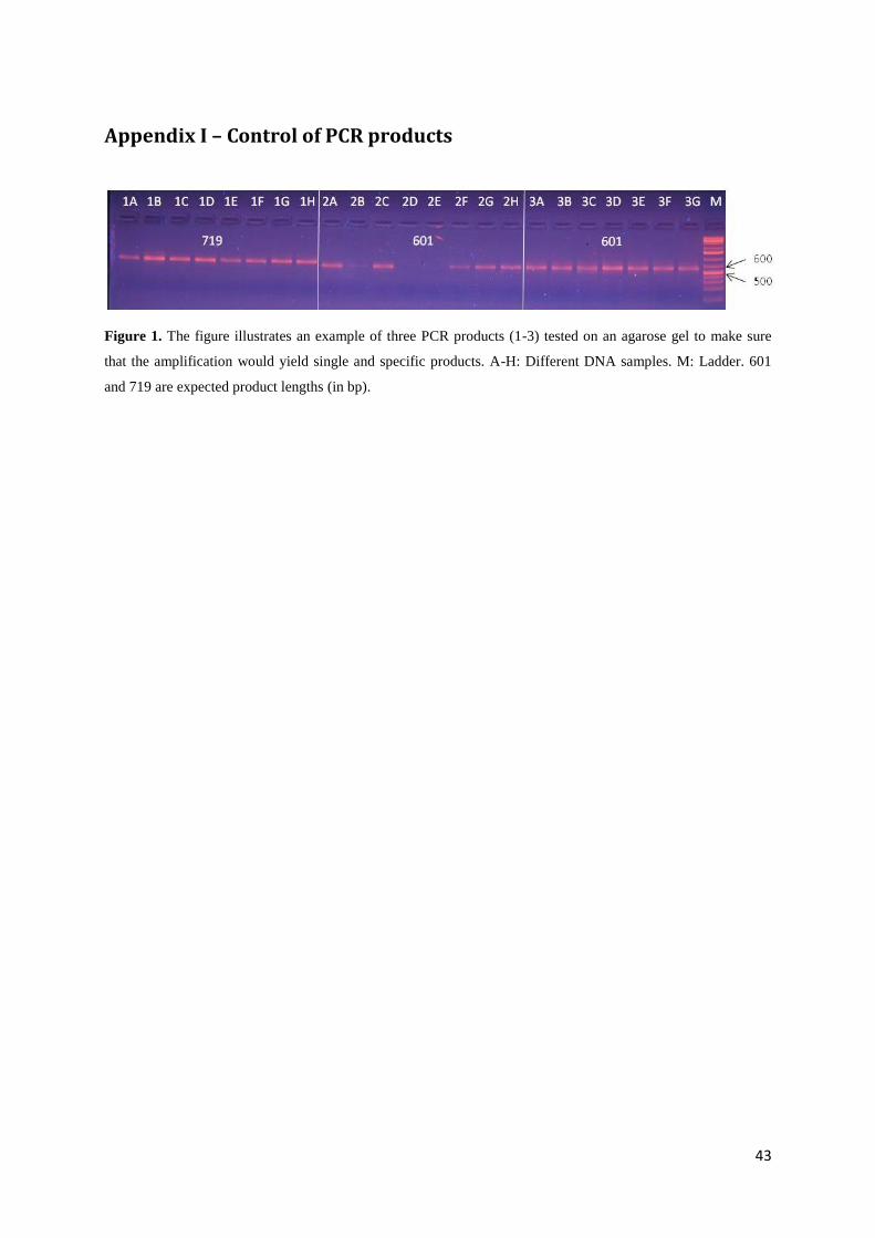
43

Appendix I – Control of PCR products

Figure 1. The figure illustrates an example of three PCR products (1-3) tested on an agarose gel to make sure

that the amplification would yield single and specific products. A-H: Different DNA samples. M: Ladder. 601

and 719 are expected product lengths (in bp).

44

Appendix II – Illustration of the phenotypic test

Figure 1. Transfer of aphids from one plant to another plant using a brush.

Figure 2. A plant with two cells (wholes) in the soil sealed with corks.

45

Appendix III – Scoring of the phenotypic test

A

C

B

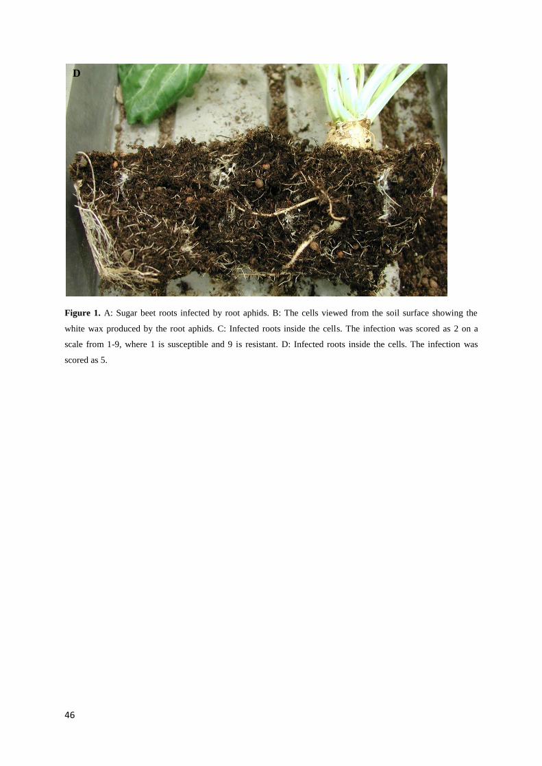
46

Figure 1. A: Sugar beet roots infected by root aphids. B: The cells viewed from the soil surface showing the

white wax produced by the root aphids. C: Infected roots inside the cells. The infection was scored as 2 on a

scale from 1-9, where 1 is susceptible and 9 is resistant. D: Infected roots inside the cells. The infection was

scored as 5.

D

fine mapping of resistance against root aphids in sugar beet · kromosom i på sockerbeta, men...

Documents