fingerprint image segmentation based on hidden markov models
TRANSCRIPT
Fingerprint Image Segmentation
Based on Hidden Markov Models
Master’s Thesis
Stefan Klein
University of Twente
University of TwenteDepartment of Electrical Engineering
Chair of Signals & SystemsEnschede, The Netherlands
Supervisors: Prof. Dr. Ir. C.H. SlumpDr. Ir. H.F.J.M. KoopmanDr. Ir. A.M. BazenDr. Ir. R.N.J. Veldhuis
Period: January 2002 - October 2002Report Code: SAS 036N02
BW 142

Samenvatting
Een belangrijke stap in vingerafdrukherkenning is de segmentatie. Tijdensde segmentatie wordt de vingerafdruk opgedeeld in voorgrond, achtergronden slechte gebieden. Duidelijke lijnstructuren, die karakteristiek zijn voorvingerafdrukken, worden gevonden in de voorgrond. De achtergrond is hetgebied waar de vinger de sensor niet heeft aangeraakt. Bewegingen vande vinger tijdens het scannen, vuil en krassen veroorzaken gebieden vanlage kwaliteit. De voorgrond wordt gebruikt in het herkenningsproces, deachtergrond wordt genegeerd. Of de slechte gebieden gebruikt worden hangtaf van de herkenningsmethode.
Zogenaamde “pixel features” van de vingerafdruk, zoals het locale gemid-delde van de grijswaarden, vormen de basis van segmentatie. De featurevector van elke pixel wordt geclassificeerd, waarbij de klasse het soort gebiedbepaalt. De meeste bestaande methoden resulteren in een gefragmenteerdesegmentatie, die door middel van postprocessing wordt gerepareerd.
Het probleem van de gefragmenteerde segmentatie wordt hier opgelostdoor gebruik te maken van een hidden Markov model (HMM). De pixelfeatures worden gemodelleerd als het uitgangssignaal van een hidden Markovproces. Het HMM zorgt ervoor dat de classificatie consistent is met die vannaburige gebieden.
De prestatie van de op een HMM gebaseerde segmentatie methode hangtsterk af van de keuze van de pixel features. In dit verslag wordt de system-atische evaluatie van een aantal pixel features beschreven.
De met een HMM verkregen segmentatie blijkt minder gefragmenteerd tezijn dan de resultaten van directe classificatie. Kwantitatieve maten wijzenook op verbetering.

Summary
An important step in fingerprint recognition is segmentation. During seg-mentation the fingerprint image is decomposed into foreground, backgroundand low-quality regions. Clear ridge-valley structures, which are characteris-tic for fingerprints, are found in the foreground. The background is the areawhere the finger did not touch the sensor. Movements of the fingertip duringscanning, dirt, and scratches cause low-quality regions. The foreground isused in the recognition process, the background is ignored. The low-qualityregions may or may not be used, dependent on the recognition method.
Pixel features of the fingerprint image, such as the local mean of thegray-values, form the basis of segmentation. The feature vector of eachpixel is classified, the class determining the region. Most of the knownmethods result in a fragmented segmentation, which is removed by meansof postprocessing.
We solve the problem of fragmented segmentation by using a hiddenMarkov model (HMM) for the classification. The pixel features are mod-elled as the output of a hidden Markov process. The HMM makes sure thatthe classification is consistent with the neighbourhood.
The performance of HMM based segmentation highly depends on thechoice of pixel features. This report describes the systematic evaluation ofa number of pixel features.
HMM based segmentation turns out to be less fragmented than directclassification. Quantitative measures also indicate improvement.


Contents
Samenvatting 3
Summary 5
1 Introduction 91.1 Background . . . . . . . . . . . . . . . . . . . . . . . . . . . . 91.2 The segmentation problem . . . . . . . . . . . . . . . . . . . . 111.3 Major issues . . . . . . . . . . . . . . . . . . . . . . . . . . . . 12
2 Hidden Markov models 152.1 Introduction . . . . . . . . . . . . . . . . . . . . . . . . . . . . 152.2 Model description . . . . . . . . . . . . . . . . . . . . . . . . . 152.3 Classification . . . . . . . . . . . . . . . . . . . . . . . . . . . 182.4 Probability of an observation sequence . . . . . . . . . . . . . 222.5 Training . . . . . . . . . . . . . . . . . . . . . . . . . . . . . . 242.6 2-D HMMs . . . . . . . . . . . . . . . . . . . . . . . . . . . . 362.7 Conclusion . . . . . . . . . . . . . . . . . . . . . . . . . . . . 38
3 Segmentation using an HMM 393.1 Introduction . . . . . . . . . . . . . . . . . . . . . . . . . . . . 393.2 Model . . . . . . . . . . . . . . . . . . . . . . . . . . . . . . . 393.3 Pixel features . . . . . . . . . . . . . . . . . . . . . . . . . . . 433.4 Conclusion . . . . . . . . . . . . . . . . . . . . . . . . . . . . 53
4 Test method 554.1 Introduction . . . . . . . . . . . . . . . . . . . . . . . . . . . . 554.2 The performance measure . . . . . . . . . . . . . . . . . . . . 554.3 The test procedure . . . . . . . . . . . . . . . . . . . . . . . . 584.4 Pixel feature selection . . . . . . . . . . . . . . . . . . . . . . 584.5 The singular point extraction test . . . . . . . . . . . . . . . . 594.6 Conclusion . . . . . . . . . . . . . . . . . . . . . . . . . . . . 62

8 Contents
5 Experimental evaluation 635.1 Introduction . . . . . . . . . . . . . . . . . . . . . . . . . . . . 635.2 Each class modelled by one state . . . . . . . . . . . . . . . . 635.3 Each class modelled by a group of states. . . . . . . . . . . . 71
6 Conclusion and recommendations 816.1 Conclusion . . . . . . . . . . . . . . . . . . . . . . . . . . . . 816.2 Recommendations . . . . . . . . . . . . . . . . . . . . . . . . 82
Acknowledgements 85
A The Viterbi algorithm 87
B The EM algorithm 89
C MATLAB functions 93
D Paper ProRISC2002 97
Bibliography 107

Chapter 1
Introduction
1.1 Background
The increasing interest in security over the last years has made that recog-nition of people by means of biometric features received more and more at-tention. Admission to restricted areas, personal identification for financialtransactions, lockers and televoting are just a few examples of applications.Many biometric characteristics can be used: iris, face, fingerprint, voice,gait etc. In practice, fingerprint is one of the easiest characteristics. Finger-print sensors are relatively low priced, no other information than necessaryis obtained and not much effort is required from the user.
Figure 1.1: A fingerprint.
In Figure 1.1 a typical fingerprint image is displayed. A common size offingerprint images is 256×364 pixels. The figure mainly consists of ridge-valley structures. Special points, like “minutiae” and “singular points”, areimportant for fingerprint recognition.
In a fingerprint verification system four main steps can be distinguished,

10 Chapter 1. Introduction
Figure 1.2: Overview of a fingerprint verification system.
see Figure 1.2. At first the fingerprint that has to be tested is scanned inthe acquisition step. After that the preprocessing takes place, which meansthat the fingerprint image is prepared for the feature extraction. In this stepthe positions of the special characteristics of the fingerprint image, such asminutiae and singular points, are determined. Then the algorithm comparesthe fingerprint to a stored template fingerprint. A sufficient match leads toacceptance of the user.
Figure 1.3: Regions that must be found by a segmentation procedure.
Subject of this report is the segmentation process, which is part of the pre-processing step. Segmentation is the decomposition of a fingerprint imageinto foreground, background and possibly low-quality regions, as is illus-trated in Figure 1.3. Clear ridge-valley structures, which are characteristicfor fingerprints, are found in the foreground. The feature extraction algo-
1.2. The segmentation problem 11
rithm is applied only to this area. The noisy background area and low-quality regions are ignored, because applying the feature extraction algo-rithm on these regions will yield false features. Further processing of theseregions may render them suitable for feature extraction or produce otherkinds of information that can be used for recognition.
From the literature several segmentation methods are known. In this re-port a method that makes use of hidden Markov models will be investigated.Unlike most existing methods, this method takes into account the context,or surroundings, for each area to be classified.
1.2 The segmentation problem
The fingerprint segmentation problem is analysed in this section. In theliterature several segmentation methods are described. In most methodsonly two classes are distinguished: foreground and background. However, itis pointed out in [4] that the use of a third class, representing low-qualityregions, may lead to better segmentation results.
The pixels, or blocks of pixels, are classified according to certain pixelfeatures, which are derived from the gray-values of the image. For example,in [15] the gradient of the gray-values in each block of 16×16 pixels is usedas a pixel feature. The ridge-valley structures in the foreground cause highervalued gradients. With this method some background parts cause problems,because the equation used for the direction computation becomes undefinedwhen the input image has perfectly uniform regions. To solve this problemthe method described in [14] uses the gray-scale variance of the block inaddition to the gradient. A region whose gray-scale variance is lower than acertain threshold is marked as background. In [22] the gray scale varianceorthogonal to the orientation of the ridges is used to classify each 16×16block. In [3] the coherence is calculated for each pixel. The coherencemeasures how well the gradients are pointing in the same direction and yieldshigh values in the foreground. In [10] the output of a set of Gabor filtersis used, which smooth the image along the direction of the line structures.A linear combination of three features is proposed in [4]. In Section 3.3 thepixel features that are tested in this report are described in detail.
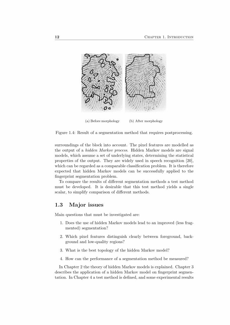
While classifying a block, none of the mentioned methods take the classesof neighbouring blocks into account. This may lead to a fragmented seg-mentation, since an image block that is surrounded by foreground blocks isvery likely to belong to the foreground too, even if the pixel features arecoincidentally typical for background area. Figure 1.4(a) shows the conse-quences [4]. Small areas that are classified as background appear withinthe foreground area. The classification estimate needs postprocessing, forexample using morphology [9]; see Figure 1.4(b).
In this report a segmentation method is presented that does take the
12 Chapter 1. Introduction
(a) Before morphology (b) After morphology
Figure 1.4: Result of a segmentation method that requires postprocessing.
surroundings of the block into account. The pixel features are modelled asthe output of a hidden Markov process. Hidden Markov models are signalmodels, which assume a set of underlying states, determining the statisticalproperties of the output. They are widely used in speech recognition [20],which can be regarded as a comparable classification problem. It is thereforeexpected that hidden Markov models can be successfully applied to thefingerprint segmentation problem.
To compare the results of different segmentation methods a test methodmust be developed. It is desirable that this test method yields a singlescalar, to simplify comparison of different methods.
1.3 Major issues
Main questions that must be investigated are:
1. Does the use of hidden Markov models lead to an improved (less frag-mented) segmentation?
2. Which pixel features distinguish clearly between foreground, back-ground and low-quality regions?
3. What is the best topology of the hidden Markov model?
4. How can the performance of a segmentation method be measured?
In Chapter 2 the theory of hidden Markov models is explained. Chapter 3describes the application of a hidden Markov model on fingerprint segmen-tation. In Chapter 4 a test method is defined, and some experimental results

1.3. Major issues 13
are presented in Chapter 5. The report is finished with conclusions and rec-ommendations. In the conclusion the four main questions are restated, andif possible, answered.
In Appendix D a paper about fingerprint image segmentation based onhidden Markov models is included, written for the ProRISC 2002 conference.

Chapter 2
Hidden Markov models
2.1 Introduction
In this chapter the theory behind hidden Markov models is explained. Firstthe model is described and the notation is defined. Then, in Section 2.3 weexplain the Viterbi algorithm, which is used for classification. An efficientprocedure for computing the probability of an observed signal is given inSection 2.4. The procedure for training the hidden Markov model’s param-eters is described in Section 2.5. Section 2.6 gives an introduction abouttwo-dimensional hidden Markov models.
2.2 Model description
A hidden Markov model (HMM) is a type of statistical signal model. Sta-tistical signal models describe the statistical properties of a signal.
Figure 2.1 shows an example of an HMM. The system can be in threestates, q1, q2, and q3, which are hidden for the observer. After a certaintime interval the system moves to another state, possibly the same state. Asequence of states that are visited during a process is notated as:
Q = Q1Q2 . . . Qt . . . QT (2.1)
The probability that state i is the initial state Q1, is called the initial stateprobability πi. The coefficients aij form a matrix A and denote the proba-bility of moving from state i to state j or staying in the same state (i = j).
π =
π1
π2
π3
where πi = P (Q1 = i) (2.2)
A =
a11 a12 a13
a21 a22 a23
a31 a32 a33
where aij = P (Qt = j|Qt−1 = i) (2.3)

16 Chapter 2. Hidden Markov models
Figure 2.1: Example of a hidden Markov model.
The output signal O is a sequence of observations:
O = O1O2 . . . Ot . . . OT (2.4)
in which Ot may be a single scalar or a vector. The statistical propertiesof this signal depend on the state of the process, so for each state j theprobability density function bj(Ot) is different.
bj(Ot) = P (Ot|Qt = j) (2.5)
Usually the probability density function is modelled by a mixture of Gaus-sian distributions:
bj(Ot) =M∑
m=1
cjmG(Ot, µjm, Σjm) (2.6)
The expression cjmG(Ot, µjm, Σjm) represents a Gaussian density functionwith mean vector µjm and covariance matrix Σjm, multiplied by a weightingfactor cjm. A mixture of M components is created, to approximate anycontinuous density function. The mixture gains cjm satisfy the followingconstraints:
M∑m=1
cjm = 1 (2.7)
cjm ≥ 0 (2.8)
If Ot is a k-dimensional vector, then µjm is a vector of k elements too andΣjm is a k × k matrix.

2.2. Model description 17
To refer to the parameters π, A, cjm, µjm and Σjm, which together com-pletely specify an HMM, a short notation is used:
λ = (π, A, c, µ,Σ) (2.9)
In Figure 2.2 a very simple 2-state HMM is displayed, which will serve asan example. The parameter set λ is defined as:
π =
[0.90.1
](2.10)
A =
[0.7 0.30.2 0.8
](2.11)
c =
[11
](2.12)
µ =[
2.0 4.0]
(2.13)
Σ =
[0.50.5
](2.14)
According to equation (2.6) the probability density functions of the ob-served signal in both states are completely defined by c, µ and Σ. Plotsof the density functions are shown in Figure 2.3. In this example they arecomposed of only one Gaussian distribution (M = 1).
Figure 2.2: A 2-state HMM.
Ot
b (O )Qt t
µ2µ1
Figure 2.3: The probability density functions in state q1 and q2.
18 Chapter 2. Hidden Markov models
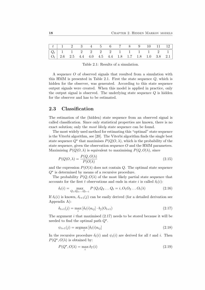
t 1 2 3 4 5 6 7 8 9 10 11 12Qt 1 1 2 2 2 2 1 1 1 1 2 1Ot 2.6 2.5 4.4 4.0 4.5 4.4 1.8 1.7 1.8 1.0 3.8 2.1
Table 2.1: Results of a simulation.
A sequence O of observed signals that resulted from a simulation withthis HMM is presented in Table 2.1. First the state sequence Q, which ishidden for the observer, was generated. According to this state sequenceoutput signals were created. When this model is applied in practice, onlythe output signal is observed. The underlying state sequence Q is hiddenfor the observer and has to be estimated.
2.3 Classification
The estimation of the (hidden) state sequence from an observed signal iscalled classification. Since only statistical properties are known, there is noexact solution; only the most likely state sequence can be found.
The most widely used method for estimating this “optimal” state sequenceis the Viterbi algorithm, see [20]. The Viterbi algorithm finds the single beststate sequence Q? that maximises P (Q|O, λ), which is the probability of thestate sequence, given the observation sequence O and the HMM parameters.Maximising P (Q|O, λ) is equivalent to maximising P (Q, O|λ), since
P (Q|O, λ) =P (Q, O|λ)P (O|λ)
(2.15)
and the expression P (O|λ) does not contain Q. The optimal state sequenceQ? is determined by means of a recursive procedure.
The probability P (Q, O|λ) of the most likely partial state sequence thataccounts for the first t observations and ends in state i is called δt(i):
δt(i) = maxQ1,Q2,...,Qt−1
P (Q1Q2 . . . Qt = i, O1O2 . . . Ot|λ) (2.16)
If δt(i) is known, δt+1(j) can be easily derived (for a detailed derivation seeAppendix A):
δt+1(j) = maxi
[δt(i)aij ] · bj(Ot+1) (2.17)
The argument i that maximised (2.17) needs to be stored because it will beneeded to find the optimal path Q?.
ψt+1(j) = argmaxi
[δt(i)aij ] (2.18)
In the recursive procedure δt(i) and ψt(i) are derived for all t and i. ThenP (Q?, O|λ) is obtained by:
P (Q?, O|λ) = maxi
δT (i) (2.19)
2.3. Classification 19
Using the information stored in ψt(j), the optimal state sequence Q? can befound. This state sequence most likely accounts for the observed signal O.
The complete Viterbi algorithm for a N -state HMM is stated here. Inaddition to the general equations, application of the Viterbi procedure on a2-state HMM is described.
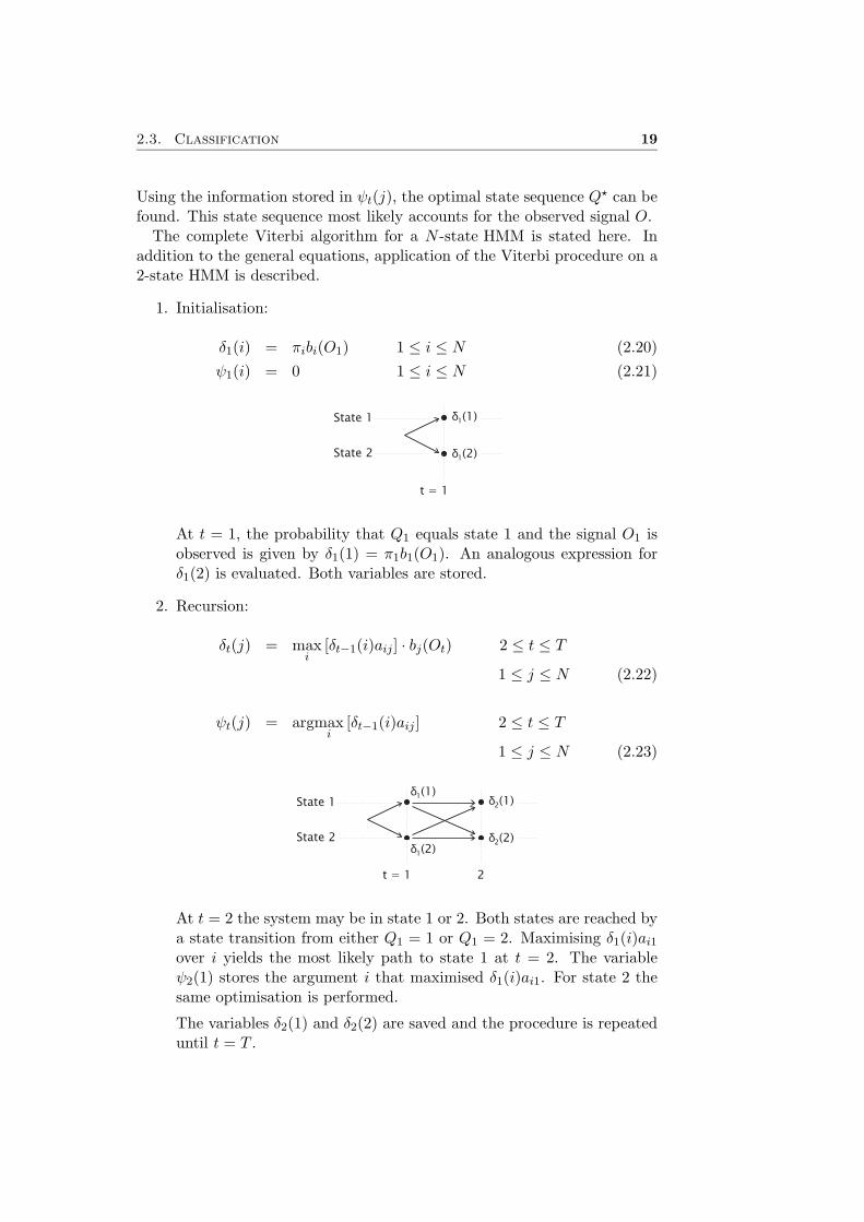
1. Initialisation:
δ1(i) = πibi(O1) 1 ≤ i ≤ N (2.20)ψ1(i) = 0 1 ≤ i ≤ N (2.21)
δ1(1)
δ1(2)
t = 1
State 1
State 2
At t = 1, the probability that Q1 equals state 1 and the signal O1 isobserved is given by δ1(1) = π1b1(O1). An analogous expression forδ1(2) is evaluated. Both variables are stored.
2. Recursion:
δt(j) = maxi
[δt−1(i)aij ] · bj(Ot) 2 ≤ t ≤ T
1 ≤ j ≤ N (2.22)
ψt(j) = argmaxi
[δt−1(i)aij ] 2 ≤ t ≤ T
1 ≤ j ≤ N (2.23)
t = 1
State 1
State 2
δ1(1)
δ1(2)
δ2(1)
δ2(2)
2
At t = 2 the system may be in state 1 or 2. Both states are reached bya state transition from either Q1 = 1 or Q1 = 2. Maximising δ1(i)ai1
over i yields the most likely path to state 1 at t = 2. The variableψ2(1) stores the argument i that maximised δ1(i)ai1. For state 2 thesame optimisation is performed.
The variables δ2(1) and δ2(2) are saved and the procedure is repeateduntil t = T .

20 Chapter 2. Hidden Markov models
3. Termination:
P (Q?, O|λ) = maxi
δT (i) (2.24)
Q?T = argmax
iδT (i) (2.25)
t = T
δT(1)
δT(2)
State 1
State 2
δT(1)δT(2) >
⇐ Q * = 2T
The maximum δ at t = T equals the probability of the most likelystate sequence Q?. The state that corresponds to this maximum δ, inthis example state 2, is the last state of Q?.
4. State sequence backtracking:
Q?t = ψt+1
(Q?
t+1
)t = T − 1, T − 2, . . . , 1 (2.26)
T-1
State 1
State 2
T
Q *T
Q *T-1
T-2
Q *T-2
Starting from Q?T , which is known, the rest of the optimal path Q?
can be found. In ψT (2) it is stored which state at t = T −1 maximisedδT (2) and thus belongs to the optimal path.
This step is repeated until Q? is determined completely. The statesequence that most likely accounts for the observed signal O has beenestimated.
To check the performance of the Viterbi estimation algorithm, the proce-dure is applied on data generated by a 2-state HMM with parameter set λ.Hundred observation sequences of length T = 40 are obtained by simulationof the model. These signals serve as an input for the Viterbi algorithm,which will estimate the underlying state sequences.
The estimation is carried out twice. First (Estimate 1), the Viterbi algo-rithm is given all parameters that defined the HMM. This means that thealgorithm knows exactly the properties of the process that generated theobserved signals. The procedure works as explained before.
The second time (Estimate 2), the Viterbi method is executed again,but without any information about the state transition probabilities of the
2.3. Classification 21
0 1 2 3 4 5 6 70
0.5
1
b (O )Qt t
Ot
b (O ) > b (O )2 t 1 t
⇐
Q = 2t
b (O ) > b (O )1 t 2 t
⇐
Q = 1t
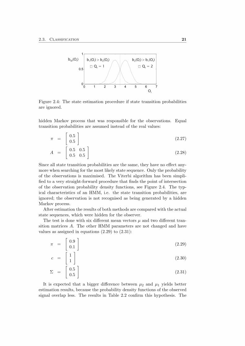
Figure 2.4: The state estimation procedure if state transition probabilitiesare ignored.
hidden Markov process that was responsible for the observations. Equaltransition probabilities are assumed instead of the real values:
π =
[0.50.5
](2.27)
A =
[0.5 0.50.5 0.5
](2.28)
Since all state transition probabilities are the same, they have no effect any-more when searching for the most likely state sequence. Only the probabilityof the observations is maximised. The Viterbi algorithm has been simpli-fied to a very straight-forward procedure that finds the point of intersectionof the observation probability density functions, see Figure 2.4. The typ-ical characteristics of an HMM, i.e. the state transition probabilities, areignored; the observation is not recognised as being generated by a hiddenMarkov process.
After estimation the results of both methods are compared with the actualstate sequences, which were hidden for the observer.
The test is done with six different mean vectors µ and two different tran-sition matrices A. The other HMM parameters are not changed and havevalues as assigned in equations (2.29) to (2.31):
π =
[0.90.1
](2.29)
c =
[11
](2.30)
Σ =
[0.50.5
](2.31)
It is expected that a bigger difference between µ2 and µ1 yields betterestimation results, because the probability density functions of the observedsignal overlap less. The results in Table 2.2 confirm this hypothesis. The
22 Chapter 2. Hidden Markov models
A =
[0.7 0.30.2 0.8
]A =
[0.9 0.10.1 0.9
]
µ = [µ1 µ2] Estimate 1Error %
Estimate 2Error %
Estimate 1Error %
Estimate 2Error %
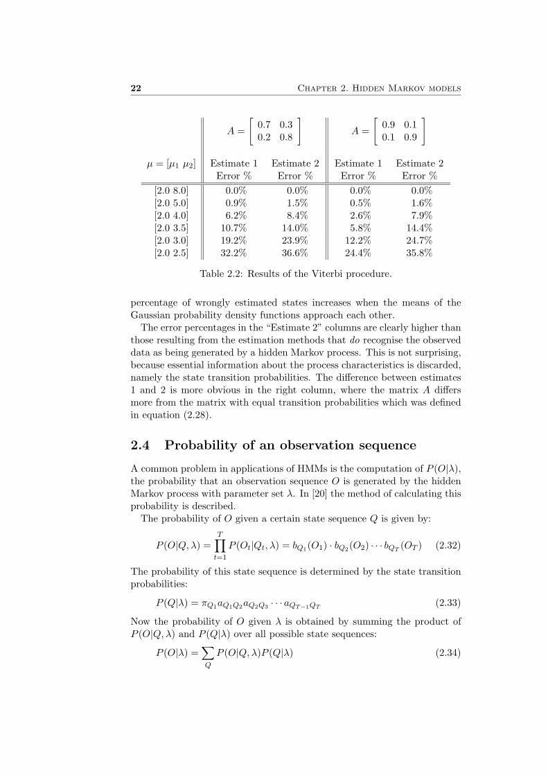
[2.0 8.0] 0.0% 0.0% 0.0% 0.0%[2.0 5.0] 0.9% 1.5% 0.5% 1.6%[2.0 4.0] 6.2% 8.4% 2.6% 7.9%[2.0 3.5] 10.7% 14.0% 5.8% 14.4%[2.0 3.0] 19.2% 23.9% 12.2% 24.7%[2.0 2.5] 32.2% 36.6% 24.4% 35.8%
Table 2.2: Results of the Viterbi procedure.
percentage of wrongly estimated states increases when the means of theGaussian probability density functions approach each other.
The error percentages in the “Estimate 2” columns are clearly higher thanthose resulting from the estimation methods that do recognise the observeddata as being generated by a hidden Markov process. This is not surprising,because essential information about the process characteristics is discarded,namely the state transition probabilities. The difference between estimates1 and 2 is more obvious in the right column, where the matrix A differsmore from the matrix with equal transition probabilities which was definedin equation (2.28).
2.4 Probability of an observation sequence
A common problem in applications of HMMs is the computation of P (O|λ),the probability that an observation sequence O is generated by the hiddenMarkov process with parameter set λ. In [20] the method of calculating thisprobability is described.
The probability of O given a certain state sequence Q is given by:
P (O|Q, λ) =T∏
t=1
P (Ot|Qt, λ) = bQ1(O1) · bQ2(O2) · · · bQT(OT ) (2.32)
The probability of this state sequence is determined by the state transitionprobabilities:
P (Q|λ) = πQ1aQ1Q2aQ2Q3 · · · aQT−1QT(2.33)
Now the probability of O given λ is obtained by summing the product ofP (O|Q, λ) and P (Q|λ) over all possible state sequences:
P (O|λ) =∑Q
P (O|Q, λ)P (Q|λ) (2.34)

2.4. Probability of an observation sequence 23
The number of possible state sequences is for a N -state HMM equal toNT . This implies that evaluation of equation (2.34) is a time-consumingtask.
The forward-backward procedure is a more efficient way of computingP (O|λ). First we define the forward variable αt(i):
αt(i) = P (O1O2 . . . Ot, Qt = i|λ) (2.35)
This variable is defined in such way that:
P (O|λ) =N∑
i=1
αT (i) (2.36)
Calculation of αt(i) requires an inductive process:
1. Initialisation:
α1(i) = πibi(O1) 1 ≤ i ≤ N (2.37)
2. Induction:
αt+1(i) =
[N∑
i=1
αt(i)aij
]bj(Ot+1) 1 ≤ t ≤ T − 1
1 ≤ j ≤ N (2.38)
3. Termination:
P (O|λ) =N∑
i=1
αT (i) (2.39)
This is a much faster way of computing P (O|λ).Likewise, we can define the backward variable βt(i):
βt(i) = P (Ot+1Ot+2 . . . OT |Qt = i, λ) (2.40)
This variable is not needed for calculation of P (O|λ), but will be used inthe next section. An inductive procedure is used again to determine βt(i):
1. Initialisation:
βT (i) = 1 1 ≤ i ≤ N (2.41)
2. Induction:
βt(i) =N∑
j=1
aijbj(Ot+1)βt+1(j) t = T − 1, T − 2, . . . , 1
1 ≤ i ≤ N (2.42)
24 Chapter 2. Hidden Markov models
The forward and backward variables have the following property, whichis valid for 1 ≤ t ≤ T :
P (Qt = i, O|λ) =∑
{Q|Qt=i}P (Q, O|λ) = αt(i)βt(i) ⇒
P (O|λ) =N∑
i=1
∑{Q|Qt=i}
P (Q, O|λ) =N∑
i=1
αt(i)βt(i) (2.43)
This property is used in the reestimation functions of the EM method, whichwill be explained in Section 2.5.2.
2.5 Training
An HMM is fully determined by the variable set λ = (π, A, c, µ,Σ). Theseparameters are not always known in advance. In this section several trainingalgorithms that try to find the parameters of the HMM are described.
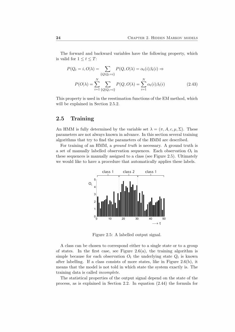
For training of an HMM, a ground truth is necessary. A ground truth isa set of manually labelled observation sequences. Each observation Ot inthese sequences is manually assigned to a class (see Figure 2.5). Ultimatelywe would like to have a procedure that automatically applies these labels.
0 10 20 30 40 500
1
2
3
4
5
t
class 1 class 2 class 1
Ot
Figure 2.5: A labelled output signal.
A class can be chosen to correspond either to a single state or to a groupof states. In the first case, see Figure 2.6(a), the training algorithm issimple because for each observation Ot the underlying state Qt is knownafter labelling. If a class consists of more states, like in Figure 2.6(b), itmeans that the model is not told in which state the system exactly is. Thetraining data is called incomplete.
The statistical properties of the output signal depend on the state of theprocess, as is explained in Section 2.2. In equation (2.44) the formula for
2.5. Training 25
(a) (b)
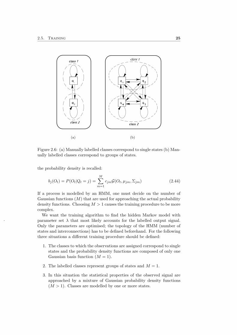
Figure 2.6: (a) Manually labelled classes correspond to single states (b) Man-ually labelled classes correspond to groups of states.
the probability density is recalled:
bj(Ot) = P (Ot|Qt = j) =M∑
m=1
cjmG(Ot, µjm, Σjm) (2.44)
If a process is modelled by an HMM, one must decide on the number ofGaussian functions (M) that are used for approaching the actual probabilitydensity functions. Choosing M > 1 causes the training procedure to be morecomplex.
We want the training algorithm to find the hidden Markov model withparameter set λ that most likely accounts for the labelled output signal.Only the parameters are optimised; the topology of the HMM (number ofstates and interconnections) has to be defined beforehand. For the followingthree situations a different training procedure should be defined:
1. The classes to which the observations are assigned correspond to singlestates and the probability density functions are composed of only oneGaussian basis function (M = 1).
2. The labelled classes represent groups of states and M = 1.
3. In this situation the statistical properties of the observed signal areapproached by a mixture of Gaussian probability density functions(M > 1). Classes are modelled by one or more states.
26 Chapter 2. Hidden Markov models
The particular training algorithm for each situation is described in the nextsections.
2.5.1 Training in situation 1
Look again at Figure 2.5 on page 24. Suppose the signal is generated by asystem that we want to model as a 2-state hidden Markov process, like isdisplayed in Figure 2.6(a). The probability distributions of the output signalin both states are approached by a single Gaussian function. We touch uponsituation 1 here since M = 1 and the labelled classes 1 and 2 correspond tosingle states of the HMM.
For each observation Ot the underlying state Qt is known. This allowsus to determine the probability distribution of the output signal (the pixelfeatures) in each state j, which is parameterised by µj and Σj . The param-eter µj equals the mean of all pixel feature vectors Ot with underlying statej. The covariance matrix Σj also follows from this set of observations. Thestate transition probabilities are obtained by counting the number of statetransitions in the labelled fingerprints. The equations for training a N -stateHMM are given by:
πi =the number of times in state i at t = 1
the number of signal sequences(2.45)
aij =the number of transitions from state i to state j
the number of transitions from state i(2.46)
cj = 1 (2.47)
µj =∑
t Ot for all t ∈ {t|Qt = j}the number of elements in {t|Qt = j} (2.48)
Σj =∑
t (Ot − µj) · (Ot − µj)T for all t ∈ {t|Qt = j}
the number of elements in {t|Qt = j} minus 1(2.49)
where equation (2.47) follows inherently from choosing M = 1.If the manually assigned labels do not correspond to single states of the
HMM, the training procedure is not that straight-forward anymore, becauseiterative estimation techniques have to be used for determining π, A, µ andΣ. This case is the subject of the next section.
2.5.2 Training in situation 2
In this section the situation that the labelled classes correspond to groupsof states is considered. The actual state that accounts for each single obser-vation is unknown. This causes the training procedure to be more complexthan the one described in Section 2.5.1.
2.5. Training 27
Suppose we have a set of observation data, each data point marked asbeing of class y (1 ≤ y ≤ Y ). It is assumed that the signal is produced bya N -state HMM and that every class y corresponds to a group of Ny statesin this HMM. Actually, the states that belong to one class form a kind of“sub-HMM”. In Figure 2.6(b) on page 25 an example is shown for Y = 2,N1 = 2, and N2 = 2.
Furthermore we assume in this section that the probability distributions ofthe output signal in all states are approached by a single Gaussian function(M = 1). Therefore, the weight factors are determined and do not need anyfurther discussion in this section:
cj = 1 1 ≤ j ≤ N (2.50)
The training procedure in this situation consists of two steps. In thefirst step the sub-HMM of each class is trained. Then, in the second step,the sub-HMMs are combined, which yields the parameters of the completehidden Markov model.
Training each class apart
The first step, training of the sub-models, will be accomplished by a com-bination of the well-known K -means clustering algorithm, which makes aninitial estimate of the parameters, and the expectation-maximisation (EM)procedure, which optimises these values.
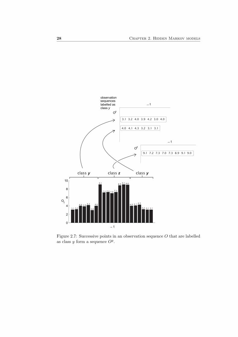
Figure 2.7 shows how successive points in an observation sequence O thatare labelled as class y form a sequence Oy. The set of signal sequencesthat is obtained in this way is assumed to be generated by the Ny statesub-HMM that models class y. For this HMM we need to estimate theparameter set λy = (πy, Ay, µy, Σy). Since the underlying state sequencesQy are unknown, the training data is called incomplete. For this kind oftraining problems, the EM algorithm can be used. Good descriptions of theEM algorithm can be found in [20] and [16].
Let us assume we have an initial estimate of λy. The EM procedure is aniterative process, which optimises λy. In every step the HMM parameters areadjusted in such a way that the probability of the observed signal, P (Oy|λy),is increased:
P (Oy|λy) > P (Oy|λy) (2.51)
where λy denotes the set of reestimated parameters. The following reestima-tion functions, which are derived in Appendix B, are used (the superscripty is omitted here for clarity):
πi =∑
{Q|Q1=i} P (O, Q|λ)∑Q P (O, Q|λ)
28 Chapter 2. Hidden Markov models
3.1 3.13.24.0 4.1 4.3
0
2
4
6
8
10
→ t
Ot
3.1 3.1 3.13.2 3.2
4.0 4.0 4.14.3
3.94.2
3.0
4.0
9.1
7.2 7.3 7.07.3
8.99.1 9.0
class y class z class y
→
→
t
t
observationsequences
labelled asclass y
O
O
y
z
3.1 3.2 4.0 3.9 4.2 3.0 4.0
9.1 7.2 7.3 7.0 7.3 8.9 9.1 9.0
Figure 2.7: Successive points in an observation sequence O that are labelledas class y form a sequence Oy.
2.5. Training 29
=α1(i)β1(i)∑N
i=1 α1(i)β1(i)(2.52)
aij =∑T
t=2
∑{Q|Qt−1=i,Qt=j} P (O, Q|λ)∑T
t=2
∑{Q|Qt−1=i} P (O, Q|λ)
=∑T
t=2 αt−1(i)aijbj(Ot)βt(j)∑Tt=2 αt−1(i)βt−1(i)
(2.53)
µj =∑T
t=1
∑{Q|Qt=j} P (O, Q|λ)Ot∑T
t=1
∑{Q|Qt=j} P (O, Q|λ)
=∑T
t=1 αt(j)βt(j)Ot∑Tt=1 αt(j)βt(j)
(2.54)
Σj =∑T
t=1
∑{Q|Qt=j} P (O, Q|λ) (Ot − µj) · (Ot − µj)
T∑Tt=1
∑{Q|Qt=j} P (O, Q|λ)
=∑T
t=1 αt(j)βt(j) (Ot − µj) · (Ot − µj)T∑T
t=1 αt(j)βt(j)(2.55)
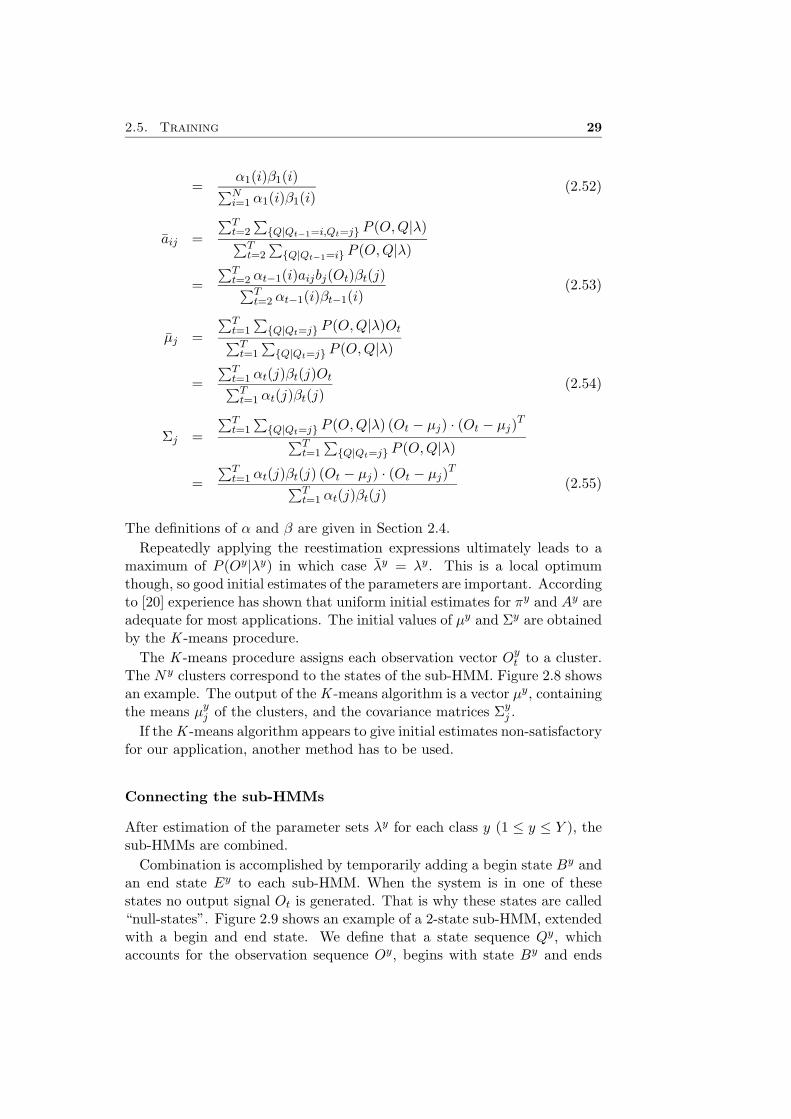
The definitions of α and β are given in Section 2.4.Repeatedly applying the reestimation expressions ultimately leads to a
maximum of P (Oy|λy) in which case λy = λy. This is a local optimumthough, so good initial estimates of the parameters are important. Accordingto [20] experience has shown that uniform initial estimates for πy and Ay areadequate for most applications. The initial values of µy and Σy are obtainedby the K -means procedure.
The K -means procedure assigns each observation vector Oyt to a cluster.
The Ny clusters correspond to the states of the sub-HMM. Figure 2.8 showsan example. The output of the K -means algorithm is a vector µy, containingthe means µy
j of the clusters, and the covariance matrices Σyj .
If the K -means algorithm appears to give initial estimates non-satisfactoryfor our application, another method has to be used.
Connecting the sub-HMMs
After estimation of the parameter sets λy for each class y (1 ≤ y ≤ Y ), thesub-HMMs are combined.
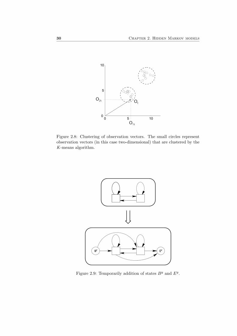
Combination is accomplished by temporarily adding a begin state By andan end state Ey to each sub-HMM. When the system is in one of thesestates no output signal Ot is generated. That is why these states are called“null-states”. Figure 2.9 shows an example of a 2-state sub-HMM, extendedwith a begin and end state. We define that a state sequence Qy, whichaccounts for the observation sequence Oy, begins with state By and ends
30 Chapter 2. Hidden Markov models
0 5 100
5
10
O1t
O2t Ot
Figure 2.8: Clustering of observation vectors. The small circles representobservation vectors (in this case two-dimensional) that are clustered by theK -means algorithm.
Figure 2.9: Temporarily addition of states By and Ey.

2.5. Training 31
with state Ey. This yields the new state sequence Qy:
Qy = ByQy1Q
y2 . . . Qy
t . . . QyT Ey (2.56)
Since the null-states do not produce any output, the observation sequencesstay the same.
The addition of the begin and end states requires adjustment of πy to πy
and Ay to Ay. By definition By is the first state of each state sequence, sothe expression for π is simple:
π =
100...0
state By
normal state 1
normal state 2
...state Ey
(2.57)
Derivation of the transition matrix is more complicated. Equation (2.58)shows the composition of A:
A =
0 [ πy ] 00 d e d e...
... Ay?...
... εy...
0 b c b c0 0 · · · 0 0
(2.58)
The vector εy is introduced first:
εyj = ay
jEy = P(Qy
t = Ey|Qyt−1 = j
)(2.59)
In fact, this expresses the probability that after being in state j the sequenceQy ends, which means that a class transition takes place. Because the statesequences are hidden (the only output of an HMM is the observed signal O),the end probabilities must be estimated. Two steps are needed to computeεy:
1. The Viterbi algorithm (Section 2.3) is carried out in order to esti-mate the most likely state sequences Qy. The input for this procedureis formed by the observation signals Oy and the parameter set λy.Adding By and Ey to the estimated state sequence yields Qy, like inequation (2.56).
2. Based on Qy the probability of transition to state Ey can be computedby counting the number of state transition occurrences:
εyj =
the number of transitions from state j to state Ey
the number of transitions from state j(2.60)
Actually this is the same expression as equation (2.46) on page 26.

32 Chapter 2. Hidden Markov models
The elements of Ay? are defined by:
ay?ij = ay
ij(1 − εyi ) 1 ≤ i, j ≤ Ny (2.61)
This guarantees that the elements of the new transition matrix Ay still obeythe standard stochastic constraints:
Ny∑j=1
ayij = 1 1 ≤ i ≤ Ny (2.62)
In the last row of Ay this constraint is not satisfied, because Ey is the laststate of each state sequence Qy. Transition to another class takes place then.
After calculation of the parameter set λy for each class y the sub-HMMsare combined, as is illustrated in Figure 2.10 for three classes (Y = 3). Theinitial state probability vector π and the transition matrix A of the completesystem are given by:
π =
πB1
0...00
πB2
0...00
πB3
0...00
state B1
normal state 1
...normal state N1
state E1
state B2
:...:state E2
state B3
:...:state E3
(2.63)

2.5. Training 33
Figure 2.10: Combination of the sub-HMMs, the null-states acting as “in-termediaries”.
34 Chapter 2. Hidden Markov models
A =
A1
...· · · 0 · · ·
...aE1B2
...· · · 0 · · ·
...aE1B3
...· · · 0 · · ·
...aE2B1
A2
...· · · 0 · · ·
...aE2B3
...· · · 0 · · ·
...aE3B1
...· · · 0 · · ·
...aE3B2
A3
(2.64)
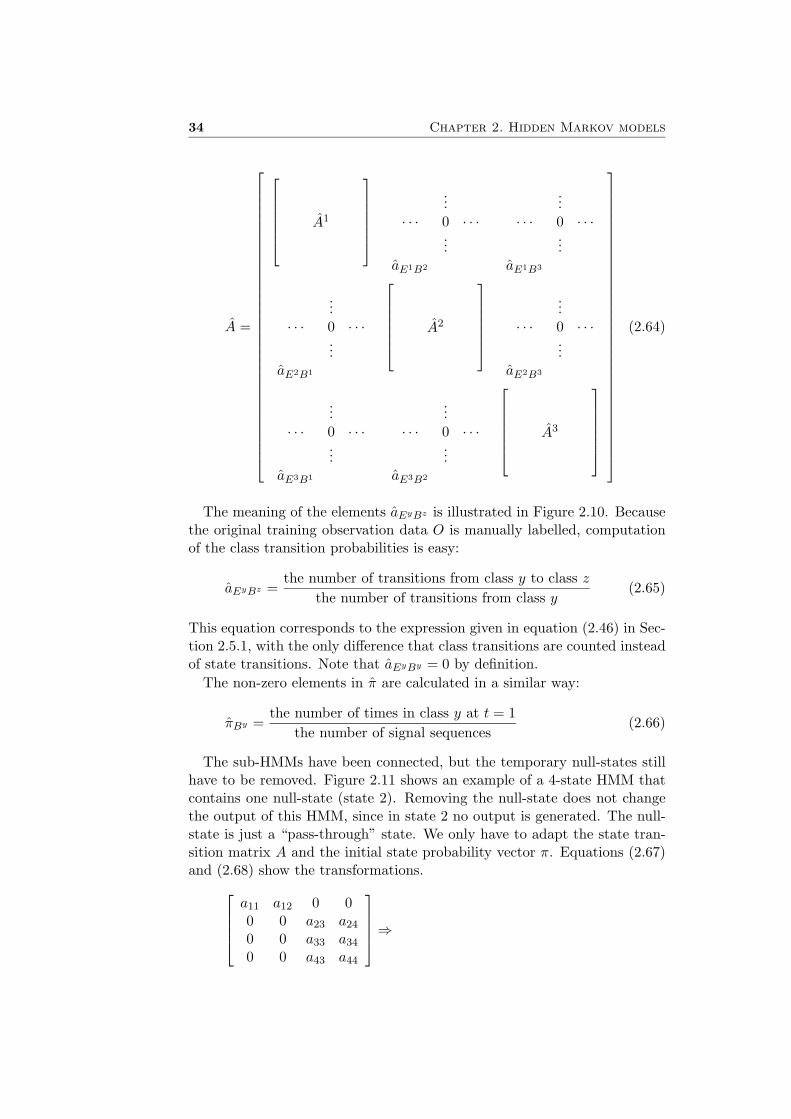
The meaning of the elements aEyBz is illustrated in Figure 2.10. Becausethe original training observation data O is manually labelled, computationof the class transition probabilities is easy:
aEyBz =the number of transitions from class y to class z
the number of transitions from class y(2.65)
This equation corresponds to the expression given in equation (2.46) in Sec-tion 2.5.1, with the only difference that class transitions are counted insteadof state transitions. Note that aEyBy = 0 by definition.
The non-zero elements in π are calculated in a similar way:
πBy =the number of times in class y at t = 1
the number of signal sequences(2.66)
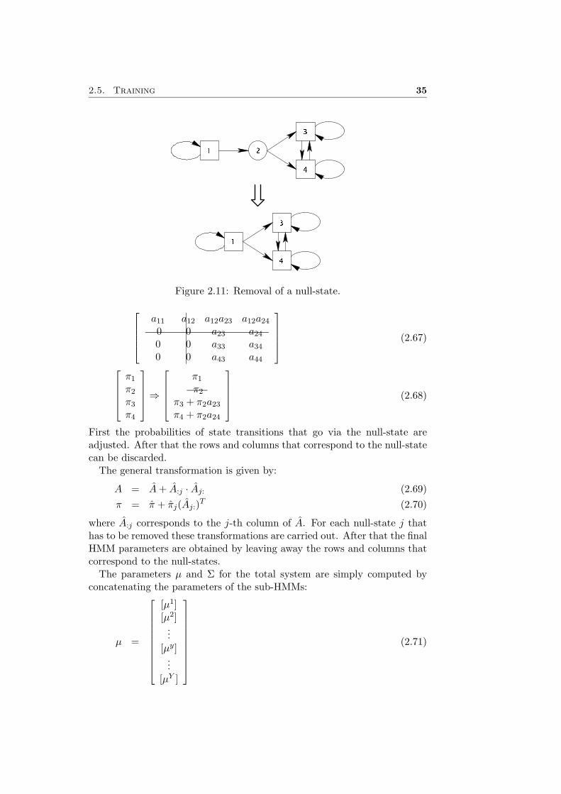
The sub-HMMs have been connected, but the temporary null-states stillhave to be removed. Figure 2.11 shows an example of a 4-state HMM thatcontains one null-state (state 2). Removing the null-state does not changethe output of this HMM, since in state 2 no output is generated. The null-state is just a “pass-through” state. We only have to adapt the state tran-sition matrix A and the initial state probability vector π. Equations (2.67)and (2.68) show the transformations.
a11 a12 0 00 0 a23 a24
0 0 a33 a34
0 0 a43 a44
⇒
2.5. Training 35
Figure 2.11: Removal of a null-state.
a11 a12 a12a23 a12a24
0 0 a23 a24
0 0 a33 a34
0 0 a43 a44
(2.67)
π1
π2
π3
π4
⇒
π1
π2
π3 + π2a23
π4 + π2a24
(2.68)
First the probabilities of state transitions that go via the null-state areadjusted. After that the rows and columns that correspond to the null-statecan be discarded.
The general transformation is given by:
A = A + A:j · Aj: (2.69)π = π + πj(Aj:)T (2.70)
where A:j corresponds to the j-th column of A. For each null-state j thathas to be removed these transformations are carried out. After that the finalHMM parameters are obtained by leaving away the rows and columns thatcorrespond to the null-states.
The parameters µ and Σ for the total system are simply computed byconcatenating the parameters of the sub-HMMs:
µ =
[µ1][µ2]...
[µy]...
[µY ]
(2.71)
36 Chapter 2. Hidden Markov models
Σ =
[Σ1][Σ2]
...[Σy]
...[ΣY ]
(2.72)
Summary
The training procedure for an HMM is explained for the situation that thelabelled classes correspond to groups of states. The training method consistsof two phases. First the observation sequences are split up, according to themanually applied labels. The groups of states that correspond to a class aretrained separately. Then, the parameters of these sub-HMMs are combinedusing the label information, which leads to the parameters of the total HMM.
In fact, after connecting the sub-HMMs, the EM algorithm could be runagain to optimise the parameters of the total HMM. Not much improvementis expected from this optimisation though.
2.5.3 Training in situation 3
In the previous section the training procedure is explained for situationsin which the statistical properties of the output signal in a certain stateare modelled by a single Gaussian density function (M = 1). The useof multiple Gaussian functions allows a better approximation of the realprobability distribution. However, the same effect is achieved by increasingthe number of states of the HMM. In fact, the two cases are mathematicallyequivalent, as is explained in [21].
We can conclude that it is useless to define a training method for thissituation, since it can be easily avoided.
2.6 2-D HMMs
The hidden Markov models that have been described in this chapter haveone-dimensional state sequences. Two-dimensional HMMs also exist. Equa-tions (2.73) and (2.74) show the difference.
1-D ⇒ Q = Q1Q2 . . . Qt . . . QT (2.73)
2-D ⇒ Q =
Q11 · · · Q1t · · · Q1T...
......
Qs1 · · · Qst · · · QsT...
......
QS1 · · · QSt · · · QST
(2.74)

2.6. 2-D HMMs 37
Several applications of 2-D HMMs are found in literature. Fields of in-terest are face recognition [19], segmentation of hand-drawn pictograms incluttered scenes [17] and aerial image segmentation [11].
In [19] and [17] pseudo 2-D hidden Markov models are used. A pseudo2-D HMM is actually a 1-D HMM that has a two-dimensional appearance.Figure 2.12 shows an example for face recognition. The HMM consists of“super states” and “embedded states”. In the case of Figure 2.12 the superstates model the image in the vertical direction and the embedded statesmodel the horizontal direction. Pseudo 2-D HMMs are mainly useful whenthe images are very predictable, like faces or documents.
Figure 2.12: A pseudo 2-D HMM, used for face recognition.
In [11] the theory of truly 2-D HMMs is explained and applied to segmen-tation of aerial images. In truly 2-D HMMs the state transition probabilitiesin the horizontal and vertical direction are both taken into account. Thiscauses the Viterbi algorithm to be more complicated. For a w × w sizedimage and a N -state HMM, the amount of computation and memory is inthe order of wNw instead of w2N in the one-dimensional case. However, anapproximation is proposed in [11], which allows the computation time to bereduced to the same order as in the one-dimensional case.
Since 2-D HMMs will not be used, further details are omitted in thisreport.

38 Chapter 2. Hidden Markov models
2.7 Conclusion
In this chapter we discussed the main aspects of the theory behind hiddenMarkov models:
• Definition of the model and the used symbols.
• Estimation of the most likely state sequence that accounts for a mea-sured sequence of observations, which is known as the classificationproblem.
• The forward-backward procedure, which allows computing the proba-bility of an observation sequence to be generated by a certain hiddenMarkov process λ.
• Training of the HMM, which is necessary to determine the parametersof the model.
Moreover, an introduction about 2-D HMMs is given.The next chapter deals with application of the theory on the problem of
fingerprint segmentation.
Chapter 3
Segmentation using an HMM
3.1 Introduction
The application of a hidden Markov model to segmentation of fingerprints isexamined. In Section 3.2 the method is explained. In Section 3.3 a numberof pixel features that may be used for segmentation is described.
3.2 Model
This section describes how the segmentation of a fingerprint can be modelledby a hidden Markov process.
Automatic segmentation is based on one or more “pixel features”, such asthe average gray-value, that are derived from the original fingerprint image.The image is partitioned in blocks of, for example, 8 × 8 pixels after whicheach block is classified.
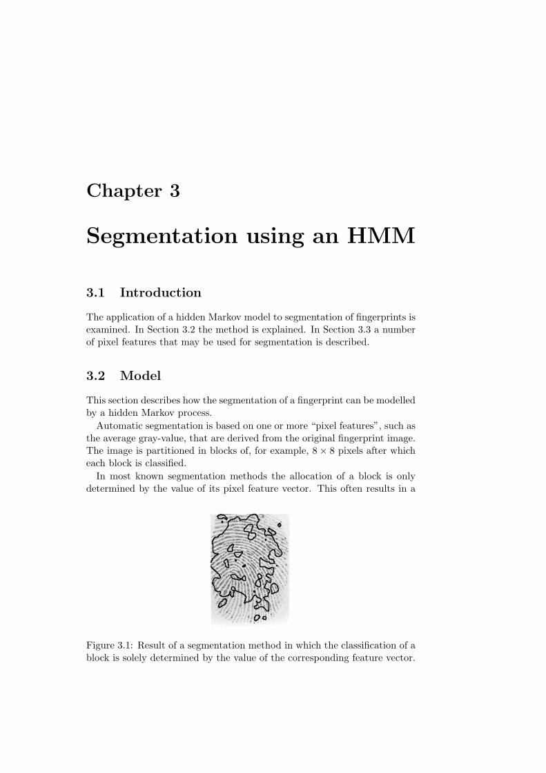
In most known segmentation methods the allocation of a block is onlydetermined by the value of its pixel feature vector. This often results in a
Figure 3.1: Result of a segmentation method in which the classification of ablock is solely determined by the value of the corresponding feature vector.
40 Chapter 3. Segmentation using an HMM
fragmented segmentation, containing many small ‘islands’ that have to beremoved by means of an appropriate postprocessing. An example is shownin Figure 3.1. A manually determined segmentation would never look likethis.
The problem of fragmentation might be prevented by taking into accountthe neighbourhood of a block during classification. We try to realise this bymeans of a hidden Markov model. As is explained in the previous chapter,a hidden Markov model consists of several states. At any time, the systemis in one of these states. Transition to another state takes place accordingto predefined transition probabilities. If we model the fingerprint in suchway that the foreground (F), background (B) and low-quality (L) regionscorrespond to states (or groups of states) in a hidden Markov process, then(properly chosen) state transition probabilities ensure a classification thatis consistent with the neighbourhood.
An illustration of the model is shown in Figure 3.2. The fingerprint isdivided in blocks of 8 × 8 pixels. Each class is modelled by one or morestates. A set of pixel features is modelled as the output of the HMM. Fromthe figure it is clear that strips of pixel feature form together the observedsignal O. Each gray-coloured strip can be seen as a sequence of observationsin “time”, see figures 3.3(a)-3.3(c). The statistical properties of these signalsare described by the probability density functions bj(Ot).
Given the observed signal O (the pixel features) and the HMM parameterset λ, the Viterbi algorithm, which is explained in Section 2.3, estimatesthe underlying state sequences Q. Accordingly, the image is segmented intoforeground, background and low-quality regions.
Note that the proposed model is one-dimensional. Each row in the imageis segmented separately. Vertical relations are ignored. As mentioned inSection 2.6, several applications of 2-D HMMs are found in the literature onimage segmentation. For now, we have chosen for a one-dimensional model,because it is easier to implement.
It depends on the complexity of the model which training algorithm isused to estimate the HMM parameters. All training methods need a set oflabelled fingerprints, like in Figure 3.4. In Section 2.5 three situations aredistinguished that lead to different training algorithms.
The third situation, in which the probability density functions bj(Ot)are approximated by a mixture of Gaussian distributions (M > 1), is notconsidered, as we explained in Section 2.5.3.
If we let the three labelled classes correspond to three HMM states, likein Figure 3.2, and use only one Gaussian density function to approach theprobability density of the pixel feature gray-values, situation 1 is obtained.In that case the training becomes very straight-forward, as is explained inSection 2.5.1. This configuration is tested in Section 5.2.
In Figure 3.5 another possible model for fingerprint segmentation is shown.In this model the foreground is modelled by two states, so the HMM of

3.2. Model 41
Figure 3.2: A fingerprint modelled by a hidden Markov process; F = fore-ground, B = background, L = low-quality area.
0.4
0.6
0.8
1
pixel feature 1
t
(a)
0
0.2
0.4
pixel feature 2
t
(b)
0.4
0.6
0.8
1
pixel feature 3
t
(c)
Figure 3.3: The gray-coloured strips are the observed output signals of theHMM that models a fingerprint.
42 Chapter 3. Segmentation using an HMM
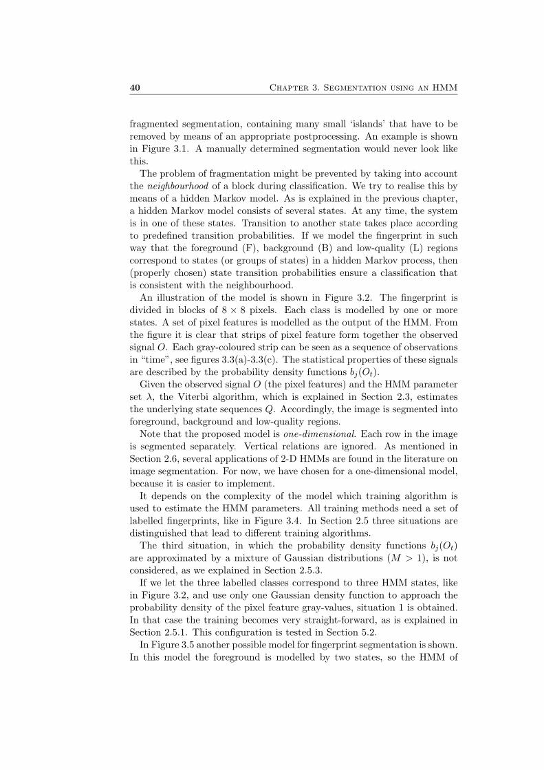
Figure 3.4: Labels are assigned to a fingerprint image.
Figure 3.2 is extended with one state, which may lead to better segmentationresults. As is explained in Section 2.5.2, the training procedure becomesmore complicated in this case, because the training data is incomplete. thetraining observation sequences are labelled, but only the classes. Thus, if aclass is modelled by more than one state, the state sequence is not knownyet after labelling.
Once the choice has been made to model a class by more than one state,many configurations become possible. For each class we need to choosethe number of states. A special configuration is investigated in this report.Suppose we have pixel features whose values are related to the orientation of
Figure 3.5: A more advanced model for fingerprint segmentation.

3.3. Pixel features 43
the line structures in the foreground. Then, it may be fruitful to subdividethe foreground into a number of states, each state corresponding to a certaindirection of the line structures. In Section 5.3 this configuration is tested.In Section 3.3.5 we will encounter pixel features that are suitable for thisconfiguration.
As mentioned before, a set of pixel features forms the output of the HMM.In the next section a number of pixel features that could be used are de-scribed.
3.3 Pixel features
3.3.1 Introduction
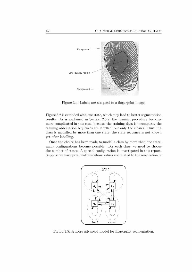
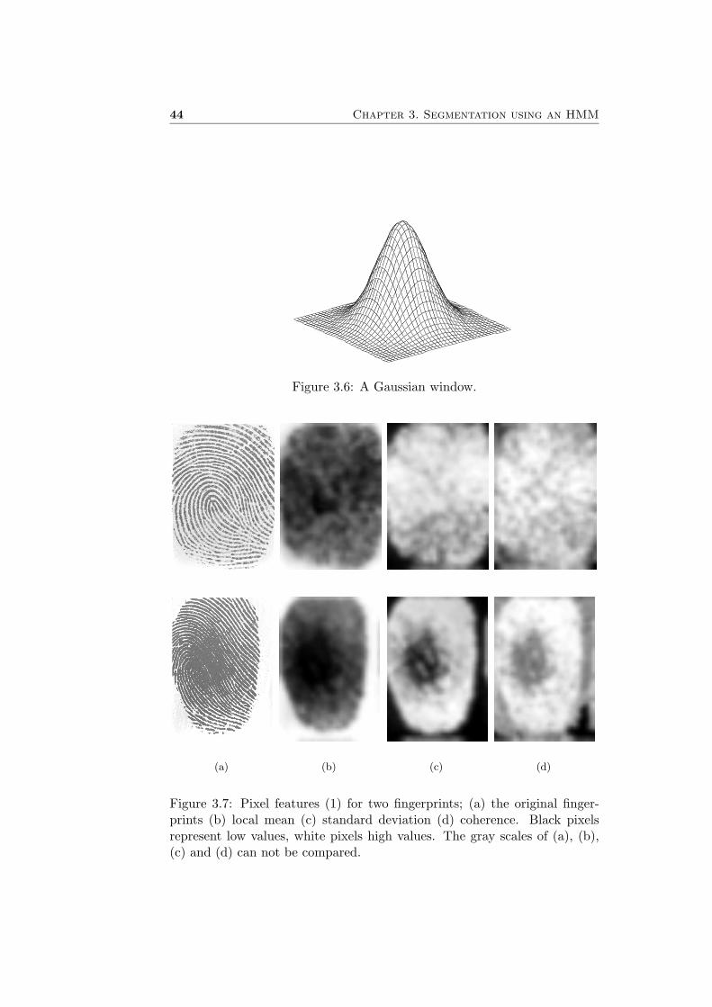
The performance of the proposed HMM based segmentation method dependshighly on the choice of pixel features. In this section an overview is givenof features that could be used for segmentation. Examples can be foundon page 44 (Figure 3.7), page 47 (Figure 3.9), page 51 (Figure 3.14), andpage 52 (Figure 3.15).
3.3.2 Local mean
Since the ridge-valley structures appear as black and white lines on thefingerprint image and the background usually is rather white, the averagegray-value of the picture may be useful for segmentation.
According to [4] the feature is calculated by applying a Gaussian filter onthe image:
Mean =∑W
I (3.1)
where I is the intensity of the image (the gray-value) and∑
W represents aGaussian window W with a standard deviation σ of 6 pixels. In Figure 3.6an example of a Gaussian window is displayed. The Gaussian window isactually a set of weighting factors, defined by equation (3.2):
h(x, y) =1
2πσ2exp
(−x2 + y2
2σ2
)(3.2)
The filtered image is obtained by applying the following procedure on eachpixel:
1. The Gaussian window is centred on the pixel.
2. The pixel gray-values of the original image are multiplied by theircorresponding weighting factors.
3. Adding up the weighted values yields the new pixel value (which is thelocal mean).
44 Chapter 3. Segmentation using an HMM
Figure 3.6: A Gaussian window.
(a) (b) (c) (d)
Figure 3.7: Pixel features (1) for two fingerprints; (a) the original finger-prints (b) local mean (c) standard deviation (d) coherence. Black pixelsrepresent low values, white pixels high values. The gray scales of (a), (b),(c) and (d) can not be compared.

3.3. Pixel features 45
Figure 3.7(b) shows the local mean values of the fingerprints displayed inFigure 3.7(a), after discretisation to blocks of 8 × 8 pixels.
3.3.3 Standard deviation
Another implication of the ridge-valley structures is that the standard de-viation of the intensity is significantly higher on the foreground than on thebackground, where the finger does not touch the sensor (see [4]).
StDev =√
(∑W
(I − Mean)2)
(3.3)
This feature is illustrated in Figure 3.7(c).
3.3.4 Coherence
The coherence is derived from the picture’s local gradients. If the gradientsare pointing in the same direction the coherence is high. A fingerprint con-sists mainly of parallel lines, so the coherence will be high in the foregroundand low in the noisy background. Figure 3.7(d) shows an example.
Equation (3.4), which is taken from [5], explains how to derive the coher-ence from the local gradient (Gx, Gy):
Coh =|∑W (Gs,x, Gs,y)|∑
W |(Gs,x, Gs,y)| =
√(Gxx − Gyy)2 + 4G2
xy
Gxx + Gyy(3.4)
(a) The originalfingerprint image
(b) The coher-ence, σ = 6
(c) The coher-ence, σ = 1
Figure 3.8: The coherence calculated with a σ of 6 pixels will lead to errorsin the core.

46 Chapter 3. Segmentation using an HMM
where (Gs,x, Gs,y) is the squared gradient and:
Gxx =∑
W G2x
Gyy =∑
W G2y
Gxy =∑
W GxGy
If the gaussian windows∑
W have a σ of 6 pixels, the difference betweenforeground and background is clear, see Figure 3.8(b). However, the singularpoint of the fingerprint (the core) gives a low coherence too, so will probablybe excluded from the foreground, which is not desirable.
Using a Gaussian window with σ = 1 and averaging the outcome of equa-tion (3.4) by means of a Gaussian window with σ = 6 leads to the picturesshown in Figure 3.8(c) and Figure 3.7(d). The problem with the core hasbeen averted.
3.3.5 Gabor response
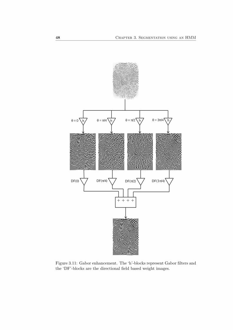
Applying an oriented Gabor filter, controlled by the directional field of thefingerprint, yields interesting information. The basic idea is that the imageis smoothed along the direction of the lines. The ridge-valley structuresbecome more clear, see Figure 3.9(b).
As explained in [2], a Gabor filter is defined by a multiplication of a cosinewith a Gaussian window:
h(x, y) = exp
(−x2 + y2
2σ2
)cos 2πf(x sin θ + y cos θ) (3.5)
where θ is the orientation of the filter, f the spatial frequency and σ thestandard deviation of the Gaussian window. An illustration of the filtercan be seen in Figure 3.10. The image is filtered in four directions, θ ={0, 1
4π, 12π, 3
4π}. The four pictures that result are combined into one image,as is shown in Figure 3.11. Before addition of the images, multiplicationwith a directional field based weight image takes place, which is explainedin [2].
For use as a pixel feature this operation is not very suitable, since it tendsto find (non-existing) ridge-valley structures in background and low-qualityregions. Scratches on a fingerprint image may transform to clear lines forexample. However, it is a good aid in visually inspecting the segmentation:the areas where Gabor enhancement goes wrong must be excluded from theforeground in the segmentation phase. In Section 4.2 more attention to thissubject is paid.
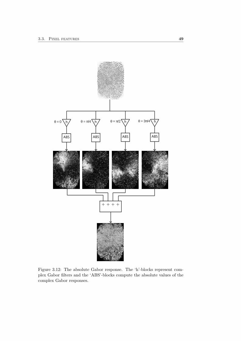
Besides the normal Gabor filter, a complex variant exists too. The com-plex Gabor filter is given by:
hCx(x, y) = exp
(−x2 + y2
2σ2
)exp (j2πf(x sin θ + y cos θ)) (3.6)

3.3. Pixel features 47
(a) (b) (c) (d)
Figure 3.9: Pixel features (2) for two fingerprints; (a) the original finger-prints (b) real part of Gabor enhanced image (c) absolute values of Gaborresponse (d) the sum of all DCT coefficients except c11. Black pixels rep-resent low values, white pixels high values. The gray scales of (a), (b), (c)and (d) can not be compared.
Figure 3.10: The impulse response of a Gabor filter.
48 Chapter 3. Segmentation using an HMM
+ + + +
θ = 0
DF( )0 DF( )π/4 DF( )π/2 DF(3 )π/4
θ = π/4 θ = π/2 θ = 3π/4h h h h
Figure 3.11: Gabor enhancement. The ‘h’-blocks represent Gabor filters andthe ‘DF’-blocks are the directional field based weight images.
3.3. Pixel features 49
+ + + +
θ = 0 θ = π/4 θ = π/2 θ = 3π/4h h h h
ABS ABS ABS ABS
Figure 3.12: The absolute Gabor response. The ‘h’-blocks represent com-plex Gabor filters and the ‘ABS’-blocks compute the absolute values of thecomplex Gabor responses.

50 Chapter 3. Segmentation using an HMM
The real part of this complex expression equals h(x, y) in equation (3.5).Figure 3.12 shows the absolute value of the complex Gabor response. Theresults of filtering in four directions are combined again, but, unlike the caseof normal Gabor filtering (Figure 3.11), weighting with the directional fieldis not necessary. The images are simply added.
Averaging by means of a Gaussian filter yields an image that may be suit-able for usage in our segmentation method. In Figure 3.9(c) two examplesare shown. Comparing Figures 3.9(c) and 3.7(c) (on page 44) leads to theconclusion that after applying the Gaussian filter the absolute values of thecomplex Gabor response give similar information as the image’s standarddeviation.
In Section 3.2 we introduced the idea of subdividing the foreground intofour states, each state corresponding to a certain direction of the line struc-tures. The four images of which the total Gabor response is composed canbe used as pixel features in this case. In Section 5.3 this configuration istested.
3.3.6 Features derived from a DCT
A discrete cosine transformation (DCT), described in [24], is widely used inimage coding. The algorithm transforms an image block P of M ×N pixelsto a linear combination of basis matrices:
P =M∑i=1
N∑j=1
cijBij (3.7)
In this equation the matrices Bij represent the basis matrices and cij arethe transform coefficients. The 64 basis matrices for a block of 8 × 8 pixels(M = N = 8) are displayed in Figure 3.13. This figure clarifies that high iand j correspond to high frequencies.
Many pixel features can be extracted from the transform coefficient ma-trix:
• For each 8 × 8 block the sum of all DCT coefficients cij except c11
is calculated. Plotting this feature, see Figure 3.9(d), clarifies thatthis measure gives similar information as the standard deviation (Fig-ure 3.7(c) on page 44).
• The elements c11 from each block, also called the DC coefficients, givethe same information as the local mean, see figures 3.14(b) and 3.7(b).
• The coefficients cij with i, j ≤ 3 are connected with the ridge-valleystructures. As is obvious in figures 3.14(c) and 3.14(d), horizontallines yield high values of |c21| and vertical lines are responsible forhigh values of |c12|. The maximum low-frequency coefficient may bea good pixel feature too. The plot in Figure 3.15(b) shows that thisfeature is quite similar to the absolute Gabor response (Figure 3.9(c)).

3.3. Pixel features 51
Figure 3.13: Basis matrices of an 8 × 8 DCT
(a) (b) (c) (d)
Figure 3.14: Pixel features (3) for two fingerprints; (a) the original fin-gerprints (b)-(d) the absolute values of the coefficients |c11|, |c21| and |c12|,obtained from discrete cosine transformation. Black pixels represent lowvalues, white pixels high values. The gray scales of (a), (b), (c) and (d) cannot be compared.
52 Chapter 3. Segmentation using an HMM
(a) (b) (c) (d)
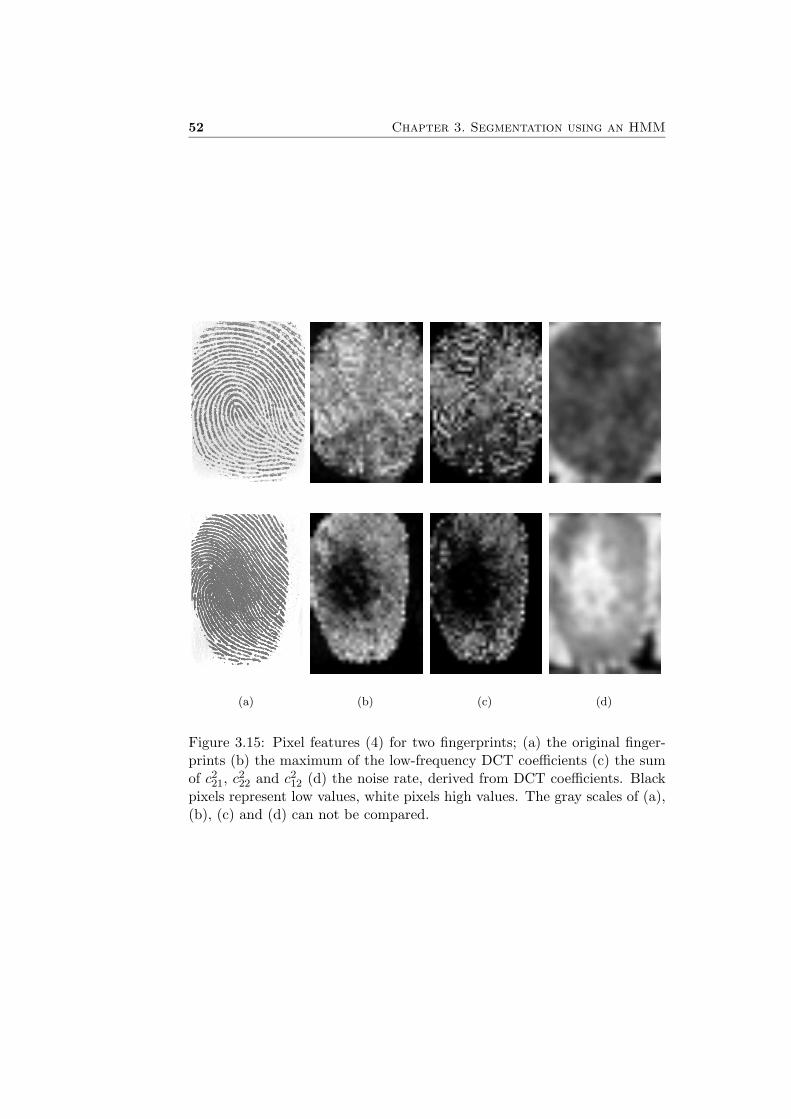
Figure 3.15: Pixel features (4) for two fingerprints; (a) the original finger-prints (b) the maximum of the low-frequency DCT coefficients (c) the sumof c2
21, c222 and c2
12 (d) the noise rate, derived from DCT coefficients. Blackpixels represent low values, white pixels high values. The gray scales of (a),(b), (c) and (d) can not be compared.

3.4. Conclusion 53
• Other interesting features may be created by adding c221, c2
22 and c212,
plotted in Figure 3.15(c), and, similar, the sum of c231, c2
32, c233, c2
23 andc213. These measures correspond to the energy in a certain frequency
band and are related to the absolute Gabor response.
• Low-quality regions and background area are characterised by bigamounts of “noise”. The high-frequency DCT components have highervalues. Thus, a measure for the noise rate can be defined as:
NoiseRate =∑W
∑i,j |cij | for 4 ≤ i, j ≤ 8
ε +∑
i,j |cij | for (i, j) 6= (1, 1)(3.8)
in which ε is a small number that prevents division by zero and W isa Gaussian window. Equation (3.8) is based on a 8 × 8 DCT. A plotis shown in Figure 3.15(d).
3.3.7 Summary
In sections 3.3.2 to 3.3.6 a number of pixel features are described that arelisted here:
1. The local mean.2. The standard deviation.3. The coherence.4. The absolute values of the complex Gabor response.5. The DC coefficient c11 that results from a discrete cosine transfor-
mation (DCT).6. The DCT coefficients |c21|, |c22| and |c12|; so actually this leads to
three pixel features.7. The DCT coefficients |c31|, |c32|, |c33|, |c23| and |c13|.8. The energy in the second frequency band (= c2
21 + c222 + c2
12).9. The energy in the third frequency band (= c2
31+c232+c2
33+c223+c2
13).10. The maximum low-frequency DCT component.11. The sum of all DCT coefficients except c11.12. The noise rate, derived from the DCT coefficients.
Twelve options are defined, which means that 212 = 4096 combinationsare possible. In the next section a method for finding the best combinationis explained.
3.4 Conclusion
In this chapter an HMM based fingerprint segmentation method is described.Each row of the fingerprint image is modelled by a hidden Markov process.

54 Chapter 3. Segmentation using an HMM
The classes foreground, background, and low-quality area correspond toone or more states in the HMM. From the pixel features, which form theoutput of the HMM, the underlying states can be estimated using the Viterbialgorithm.
The next chapter describes a test method, for evaluation of different con-figurations of our segmentation method. Also a systematic method for se-lection of the best combination of pixel features is developed.
Chapter 4
Test method
4.1 Introduction
From the previous chapter it becomes clear that many configurations arepossible when performing the segmentation using a hidden Markov model.The topology of the HMM must be chosen (number of states and intercon-nections) and a good combination of pixel features. To compare all differentconfigurations, we need to define a test procedure.
4.2 The performance measure
Checking the performance of a segmentation can be done in several ways.The final goal of segmentation is to improve the fingerprint recognition per-formance. Thus, a way to measure the effectiveness of a segmentation al-gorithm would be to carry out a fingerprint recognition test. Recognitionperformance indicates whether the segmentation algorithm is good or not.However, carrying out a complete fingerprint recognition test introduces alot of new uncertainties.
A very straight-forward way to check the performance is visual inspection.The human brain’s pattern recognition skills allow direct segmentation ofa fingerprint image. Manual segmentation can be simplified by watchingthe Gabor response of the fingerprint, a procedure that is explained in Sec-tion 3.3.5. The Gabor enhanced picture shows which parts of a fingerprintimage cause problems for the computer (see Figure 4.1). These regionsshould be excluded from the foreground area; especially because the Gaborenhanced image is used for extracting minutiae, which are the bases of manyfingerprint matching systems, as is described in [2].
A big disadvantage of visually checking the results is that automatic test-ing of many segmentation methods on a big set of fingerprints is impossible.It will take too much time. Besides that, visual inspection is subjective. A

56 Chapter 4. Test method
(a) The original fingerprint (b) The fingerprint afterGabor enhancement
Figure 4.1: Gabor enhancement shows which regions cause problems.
single scalar indicating the segmentation performance, calculated automat-ically, is preferred.
Since fingerprint segmentation is a classification problem, the results canbe summarised in a confusion matrix. From this confusion matrix a measurecan be extracted by applying a Bayesian Risk Analysis. The results of manydifferent HMM configurations can be compared easily with this measure.
A confusion matrix stores a set of probabilities that provide informationabout the performance of the classification procedure. In Table 4.1 a con-fusion matrix for the fingerprint segmentation problem is displayed. Theestimated classification is compared to the manual segmentation that hasbeen determined before (the “real classes”). Obviously, the more the matrixapproaches the identity matrix, the better the automatic segmentation.
Real classesF B L
estimated F P (F |F ) P (F |B) P (F |L)classes B P (B|F ) P (B|B) P (B|L)
L P (L|F ) P (L|B) P (L|L)
Table 4.1: The confusion matrix that summarises the segmentation results.
Although this matrix gives a good indication about segmentation perfor-mance, a single scalar should be extracted from this matrix to allow com-
4.2. The performance measure 57
parison of many results. A Bayesian Risk Analysis leads to a well-definedmeasure, called ϑ. The elements of the confusion matrix are combined withthe class frequencies P (F ), P (B) and P (L) and a cost matrix C:
ϑ =(P (F |F )CF |F + P (B|F )CB|F + P (L|F )CL|F
)· P (F ) + . . .(
P (F |B)CF |B + P (B|B)CB|B + P (L|B)CL|B)· P (B) + . . .(
P (F |L)CF |L + P (B|L)CB|L + P (L|L)CL|L)· P (L) (4.1)
where the cost matrix C denotes the “costs” of a wrong estimation.
C =
CF |F CF |B CF |LCB|F CB|B CB|LCL|F CL|B CL|L
(4.2)
The elements on the diagonal are equal to zero, because a correct estimationdoes not lead to any “costs”. Since it is important to prevent that back-ground area or low-quality regions are marked as foreground, a bigger costis assigned to these estimation errors. The following cost matrix is used:
C =
0 3 6
1 0 61 2 0
(4.3)
Of course the choice of the exact values is quite arbitrarily; different C-matrices are possible. If the aim of segmentation changes, for example ifone is only interested in finding the background area, the cost matrix willhave to be changed too.
The measure for performance measurement has been defined now. Thelower this measure, the more the automatic segmentation resembles the man-ually applied labels. However, the measure can only be used for comparingdifferent methods; it is a relative measure. On its own, it does not tell usanything about the performance of a segmentation method.
A more meaningful measure is the ratio of pixels that are assigned to thecorrect class:
P (correct) = P (F |F )P (F ) + P (B|B)P (B) + P (L|L)P (L) (4.4)
In fact, the probability of incorrect assignment, 1 − P (correct), equals theBayesian risk measure ϑ calculated with a cost matrix C = 1 − I, where Idenotes the identity matrix.
A disadvantage of this measure is that the value is mainly dominated byP (F |F )P (F ), since in most fingerprint images the foreground is the biggestarea.
58 Chapter 4. Test method
4.3 The test procedure
In order to calculate ϑ for a certain configuration of the segmentation method,four steps must be carried out:
1. Two sets of fingerprint images, the training set Straining and the testset Stest, are manually segmented (this step has to be done only once).
2. The HMM is trained on Straining, which yields the HMM parameterset λ.
3. The fingerprints in the test set Stest are partitioned in foreground,background and low-quality regions by the HMM based segmentationprocedure.
4. The segmentation results are compared with the manual classificationby calculating the confusion matrix and performing a Bayesian RiskAnalysis. This yields the performance measure ϑ.
Tests are done using MATLAB. An HMM toolbox [18] is used, whichcontains standard functions for the K -means procedure, the EM algorithm,and the Viterbi algorithm (see Chapter 2).
The fingerprints that are used for training and testing are taken fromdatabase 2 of the Fingerprint Verification Competition (FVC2000), see [12].This database consists of 880 fingerprint images, acquired from untrainedvolunteers using a capacitive sensor. The training set Straining consists of69 fingerprint images from the database. The test set Stest is composedof 43 different images. Both sets stay the same in all tests, to allow faircomparison of different configurations.
4.4 Pixel feature selection
In Section 3.3 we proposed twelve pixel features. As is explained this yields4096 possible combinations. Since it takes approximately 30 seconds to carryout steps 2, 3 and 4 on a Pentium III 1GHz, it will take 34 hours to check allcombinations. If the topology of the HMM is changed, another combinationof pixel features may be optimal, so again all 4096 possibilities have to bechecked. This will take a lot of time.
In order to find the optimal combination of pixel features more fast, a ge-netic algorithm [13] may be successfully applied here. In a genetic algorithmthe solution of a problem is considered as an organism in a population. Theparameters that characterise an organism are represented by genes, storedtogether in a chromosome. The genetic algorithm begins with creating aninitial population of Npop organisms. The costs of the results of these solu-tions are computed and the organisms are sorted according to their costs.
4.5. The singular point extraction test 59
The least effective organisms are discarded (selection) and the best solutionsare combined by means of cross-over (mating) to return the population sizeto Npop. The chromosomes of the new organisms are now mutated by ran-domly altering genes with a certain probability, defined by the mutationrate. For the new population the costs are computed again and the processrepeats itself. After a number of generations the organisms in the populationbecome better and better.
The genetic algorithm can be easily applied to the pixel feature selectionproblem. In the genetic algorithm a combination of pixel features is repre-sented by an organism. A sequence of twelve bits, having value zero or one,equals the chromosome that defines the organism. Each gene, which is a bitin the chromosome, indicates if a pixel feature is either used (1) or not used(0).
The initial population is created randomly. For the size of the populationwe choose Npop = 50. For every organism (combination of pixel features)the segmentation performance measure ϑ is computed. The half of thepopulation that has the highest values of ϑ is discarded every generation.The other half is allowed to mate. The mutation rate is set to 1%.
By using this genetic algorithm the optimal combination of pixel features,given the other parameters of the HMM segmentation method, is found muchfaster, since the algorithm automatically converges to the better solutions.
4.5 The singular point extraction test
As mentioned in Section 4.2, actually we would like to check the performanceof the segmentation method by carrying out a full fingerprint recognitiontest. The singular point extraction test, which is described in [4], is a firstapproach to this.
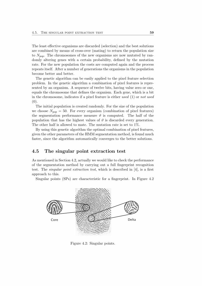
Singular points (SPs) are characteristic for a fingerprint. In Figure 4.2
Core Delta
Figure 4.2: Singular points.
60 Chapter 4. Test method
(a) Core (b) Delta
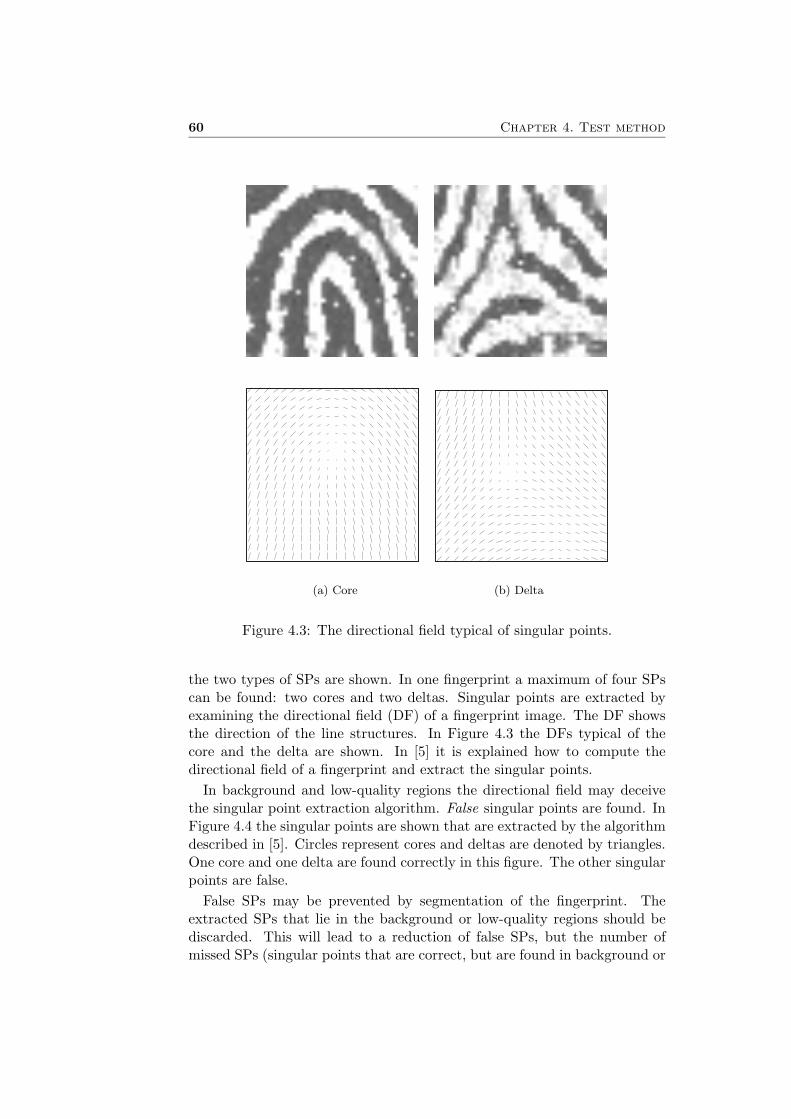
Figure 4.3: The directional field typical of singular points.
the two types of SPs are shown. In one fingerprint a maximum of four SPscan be found: two cores and two deltas. Singular points are extracted byexamining the directional field (DF) of a fingerprint image. The DF showsthe direction of the line structures. In Figure 4.3 the DFs typical of thecore and the delta are shown. In [5] it is explained how to compute thedirectional field of a fingerprint and extract the singular points.
In background and low-quality regions the directional field may deceivethe singular point extraction algorithm. False singular points are found. InFigure 4.4 the singular points are shown that are extracted by the algorithmdescribed in [5]. Circles represent cores and deltas are denoted by triangles.One core and one delta are found correctly in this figure. The other singularpoints are false.
False SPs may be prevented by segmentation of the fingerprint. Theextracted SPs that lie in the background or low-quality regions should bediscarded. This will lead to a reduction of false SPs, but the number ofmissed SPs (singular points that are correct, but are found in background or
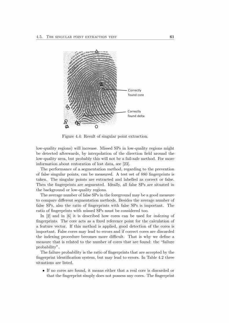
4.5. The singular point extraction test 61
Correctly
found core
Correctly
found delta
Figure 4.4: Result of singular point extraction.
low-quality regions) will increase. Missed SPs in low-quality regions mightbe detected afterwards, by interpolation of the direction field around thelow-quality area, but probably this will not be a fail-safe method. For moreinformation about restoration of lost data, see [23].
The performance of a segmentation method, regarding to the preventionof false singular points, can be measured. A test set of 880 fingerprints istaken. The singular points are extracted and labelled as correct or false.Then the fingerprints are segmented. Ideally, all false SPs are situated inthe background or low-quality regions.
The average number of false SPs in the foreground may be a good measureto compare different segmentation methods. Besides the average number offalse SPs, also the ratio of fingerprints with false SPs is important. Theratio of fingerprints with missed SPs must be considered too.
In [2] and in [6] it is described how cores can be used for indexing offingerprints. The core acts as a fixed reference point for the calculation ofa feature vector. If this method is applied, good detection of the cores isimportant. False cores may lead to errors and if correct cores are discardedthe indexing procedure becomes more difficult. That is why we define ameasure that is related to the number of cores that are found: the “failureprobability”.
The failure probability is the ratio of fingerprints that are accepted by thefingerprint identification system, but may lead to errors. In Table 4.2 threesituations are listed.
• If no cores are found, it means either that a real core is discarded orthat the fingerprint simply does not possess any cores. The fingerprint
62 Chapter 4. Test method
Nr. of cores Action
0 Accept fingerprint1 or 2 Accept fingerprint>2 Reject fingerprint or do not
use cores for verification
Table 4.2: If more than two cores are found, at least one of them is a falsecore.
identification system must use another way for registering the finger-print. In the case that a real core was discarded, because it was foundin the background or in a low-quality region, the indexing procedurehas been complicated unnecessarily.
• If the singular point extraction algorithm finds one or two cores, thefingerprint image will be accepted and the indexing procedure, whichis based on the position of the cores, is executed. This may lead toerrors since both cores could be false cores.
• If more than two cores are found, it is clear that at least one of themmust be a false core. A new fingerprint image (of higher quality)should be obtained, or the indexing must be done without using thecores.
The probability of failure can be expressed as:
P (failure) = P (CM > 0 ∧ CT = 0 ∧ CF = 0) . . .
+P (CF = 2 ∧ CT = 0) . . .
+P (CF = 1 ∧ (CT = 0 ∨ CT = 1)) (4.5)
where CF represents the number of false cores that are extracted, CT thenumber of correct cores (“true cores”), and CM the number of missed cores(correct cores that are found in the background or in low-quality regions).
The singular point extraction test takes too much time to use as a selec-tion criterion for the pixel features, but may give a good impression of theusability of the segmentation method when it is integrated in a fingerprintverification system.
4.6 Conclusion
A test procedure has been defined in this chapter, which allows objectivecomparison of many configurations of the segmentation method. In Chap-ter 3 a number of pixel features has been proposed. In Section 4.4 a sys-tematic method for selection of the best combination has been developed.
Some results of the segmentation method are presented in the next chap-ter.

Chapter 5
Experimental evaluation
5.1 Introduction
The test procedure as described in Chapter 4 is carried out, in order tofind the best configuration of the segmentation method. Some results arepresented in this chapter. In addition, the results of segmentation usinghidden Markov models are compared with the segmentation obtained by amethod that is not based on an HMM.
In Section 5.2 the test results of segmentation using a 3-state HMM arepresented. Each class is modelled by one state. In Section 5.3 the classesare modelled by more than one state.
5.2 Each class modelled by one state
5.2.1 Description
At first a simple configuration is used. Foreground, background, and thelow-quality class are all modelled by one state in the HMM.
5.2.2 Results
The genetic algorithm is executed to find a good combination of pixel fea-tures. Figure 5.1 shows the convergence of the genetic algorithm. Everygeneration the average performances of the organisms in the population im-prove. The combinations of pixel features become better.
It appears that in almost all of the best combinations the local mean,the standard deviation, the coherence and the absolute value of the Gaborresponse are used as pixel features. In addition to these four features, otherpixel features are used. These combinations yield a slightly lower ϑ, butvisual inspection shows that they do not lead to any significant segmentationimprovement. The rest of the tests in this section are based on a combination
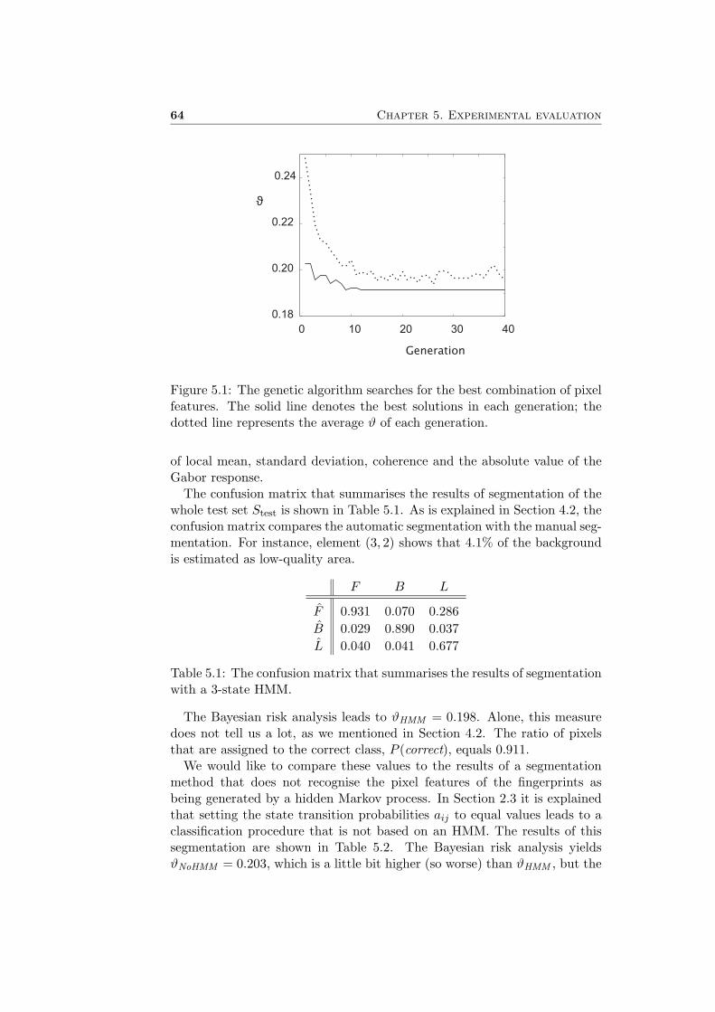
64 Chapter 5. Experimental evaluation
0 10 20 30 40
0.18
0.20
0.22
0.24
Generation
ϑ
Figure 5.1: The genetic algorithm searches for the best combination of pixelfeatures. The solid line denotes the best solutions in each generation; thedotted line represents the average ϑ of each generation.
of local mean, standard deviation, coherence and the absolute value of theGabor response.
The confusion matrix that summarises the results of segmentation of thewhole test set Stest is shown in Table 5.1. As is explained in Section 4.2, theconfusion matrix compares the automatic segmentation with the manual seg-mentation. For instance, element (3, 2) shows that 4.1% of the backgroundis estimated as low-quality area.
F B L
F 0.931 0.070 0.286B 0.029 0.890 0.037L 0.040 0.041 0.677
Table 5.1: The confusion matrix that summarises the results of segmentationwith a 3-state HMM.
The Bayesian risk analysis leads to ϑHMM = 0.198. Alone, this measuredoes not tell us a lot, as we mentioned in Section 4.2. The ratio of pixelsthat are assigned to the correct class, P (correct), equals 0.911.
We would like to compare these values to the results of a segmentationmethod that does not recognise the pixel features of the fingerprints asbeing generated by a hidden Markov process. In Section 2.3 it is explainedthat setting the state transition probabilities aij to equal values leads to aclassification procedure that is not based on an HMM. The results of thissegmentation are shown in Table 5.2. The Bayesian risk analysis yieldsϑNoHMM = 0.203, which is a little bit higher (so worse) than ϑHMM , but the

5.2. Each class modelled by one state 65
difference is very small. The ratio of pixels that are assigned to the correctclass equals 0.885.
F B L
F 0.892 0.035 0.228B 0.029 0.899 0.033L 0.079 0.075 0.739
Table 5.2: The confusion matrix that summarises the results of segmentationwithout an HMM.
In Table 5.3 the difference between the two confusion matrices is displayed(“HMM” minus “No HMM”). In the second row the differences appear to benegligible. The main differences can be found in the first and the third row.Without HMM less foreground regions are recognised as being foreground.However, less low-quality regions are estimated as foreground. From thethird row it becomes clear that the segmentation without HMM marks moreregions as being of low-quality. We can conclude that the confusion matricesdo not show us clearly which method is better.
F B L
F 0.039 0.035 0.059B 0.000 0.000 0.004L −0.040 −0.035 −0.062
Table 5.3: The difference between the confusion matrices: “HMM” minus“No HMM”.
Both methods result in a high rate (about 25%) of low-quality regions thatare estimated as foreground. Visually comparing the manual segmentation
Scratch
Figure 5.2: Scratches are not recognised.
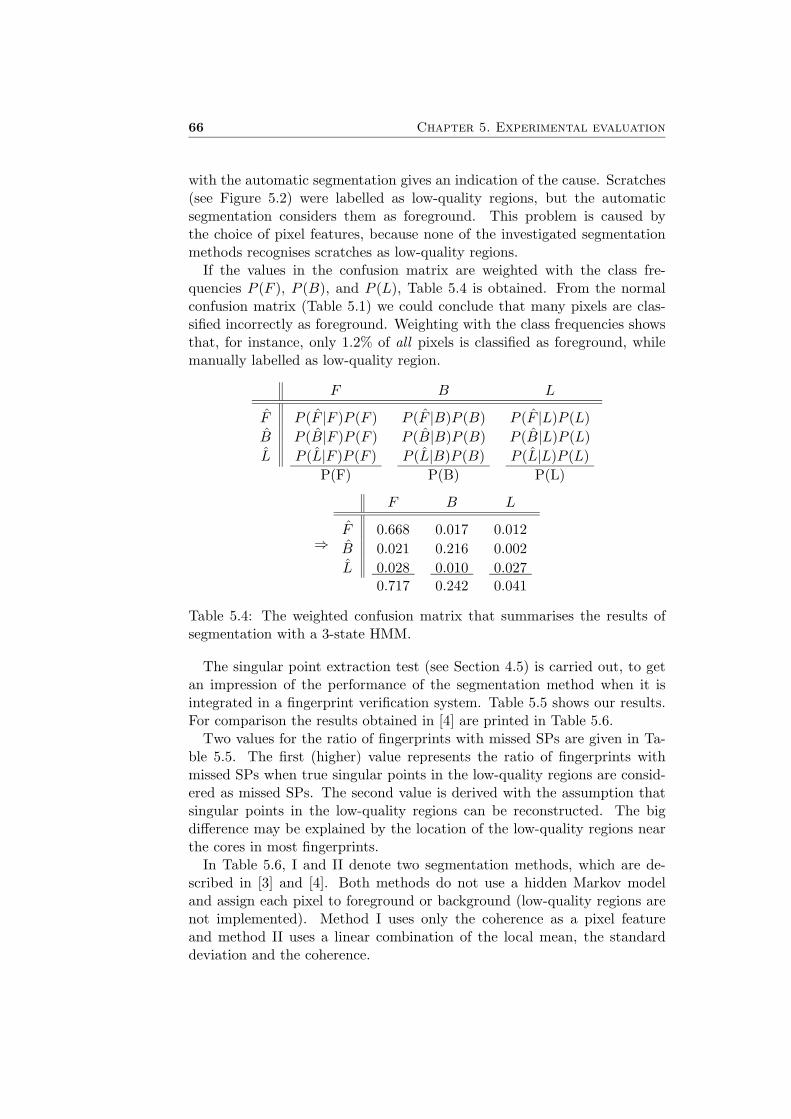
66 Chapter 5. Experimental evaluation
with the automatic segmentation gives an indication of the cause. Scratches(see Figure 5.2) were labelled as low-quality regions, but the automaticsegmentation considers them as foreground. This problem is caused bythe choice of pixel features, because none of the investigated segmentationmethods recognises scratches as low-quality regions.
If the values in the confusion matrix are weighted with the class fre-quencies P (F ), P (B), and P (L), Table 5.4 is obtained. From the normalconfusion matrix (Table 5.1) we could conclude that many pixels are clas-sified incorrectly as foreground. Weighting with the class frequencies showsthat, for instance, only 1.2% of all pixels is classified as foreground, whilemanually labelled as low-quality region.
F B L
F P (F |F )P (F ) P (F |B)P (B) P (F |L)P (L)B P (B|F )P (F ) P (B|B)P (B) P (B|L)P (L)L P (L|F )P (F ) P (L|B)P (B) P (L|L)P (L)
P(F) P(B) P(L)
⇒
F B L
F 0.668 0.017 0.012B 0.021 0.216 0.002L 0.028 0.010 0.027
0.717 0.242 0.041
Table 5.4: The weighted confusion matrix that summarises the results ofsegmentation with a 3-state HMM.
The singular point extraction test (see Section 4.5) is carried out, to getan impression of the performance of the segmentation method when it isintegrated in a fingerprint verification system. Table 5.5 shows our results.For comparison the results obtained in [4] are printed in Table 5.6.
Two values for the ratio of fingerprints with missed SPs are given in Ta-ble 5.5. The first (higher) value represents the ratio of fingerprints withmissed SPs when true singular points in the low-quality regions are consid-ered as missed SPs. The second value is derived with the assumption thatsingular points in the low-quality regions can be reconstructed. The bigdifference may be explained by the location of the low-quality regions nearthe cores in most fingerprints.
In Table 5.6, I and II denote two segmentation methods, which are de-scribed in [3] and [4]. Both methods do not use a hidden Markov modeland assign each pixel to foreground or background (low-quality regions arenot implemented). Method I uses only the coherence as a pixel featureand method II uses a linear combination of the local mean, the standarddeviation and the coherence.
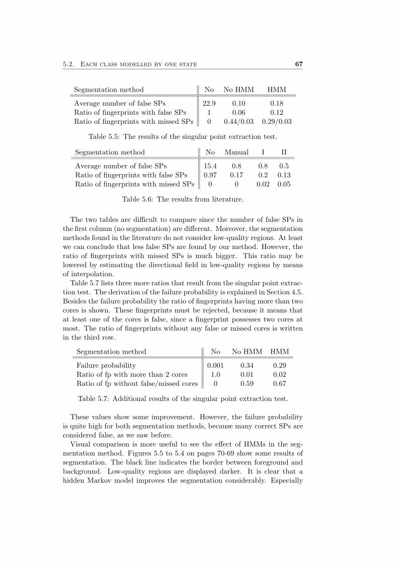
5.2. Each class modelled by one state 67
Segmentation method No No HMM HMM
Average number of false SPs 22.9 0.10 0.18Ratio of fingerprints with false SPs 1 0.06 0.12Ratio of fingerprints with missed SPs 0 0.44/0.03 0.29/0.03
Table 5.5: The results of the singular point extraction test.
Segmentation method No Manual I II
Average number of false SPs 15.4 0.8 0.8 0.5Ratio of fingerprints with false SPs 0.97 0.17 0.2 0.13Ratio of fingerprints with missed SPs 0 0 0.02 0.05
Table 5.6: The results from literature.
The two tables are difficult to compare since the number of false SPs inthe first column (no segmentation) are different. Moreover, the segmentationmethods found in the literature do not consider low-quality regions. At leastwe can conclude that less false SPs are found by our method. However, theratio of fingerprints with missed SPs is much bigger. This ratio may belowered by estimating the directional field in low-quality regions by meansof interpolation.
Table 5.7 lists three more ratios that result from the singular point extrac-tion test. The derivation of the failure probability is explained in Section 4.5.Besides the failure probability the ratio of fingerprints having more than twocores is shown. These fingerprints must be rejected, because it means thatat least one of the cores is false, since a fingerprint possesses two cores atmost. The ratio of fingerprints without any false or missed cores is writtenin the third row.
Segmentation method No No HMM HMM
Failure probability 0.001 0.34 0.29Ratio of fp with more than 2 cores 1.0 0.01 0.02Ratio of fp without false/missed cores 0 0.59 0.67
Table 5.7: Additional results of the singular point extraction test.
These values show some improvement. However, the failure probabilityis quite high for both segmentation methods, because many correct SPs areconsidered false, as we saw before.
Visual comparison is more useful to see the effect of HMMs in the seg-mentation method. Figures 5.5 to 5.4 on pages 70-69 show some results ofsegmentation. The black line indicates the border between foreground andbackground. Low-quality regions are displayed darker. It is clear that ahidden Markov model improves the segmentation considerably. Especially

68 Chapter 5. Experimental evaluation
(a) (b) (c) (d)
Figure 5.3: Results compared to the manually assigned labels and to theGabor filtered fingerprint; (a) segmentation with HMM (b) segmentationwithout HMM (c) manual segmentation (d) Gabor enhanced fingerprint.
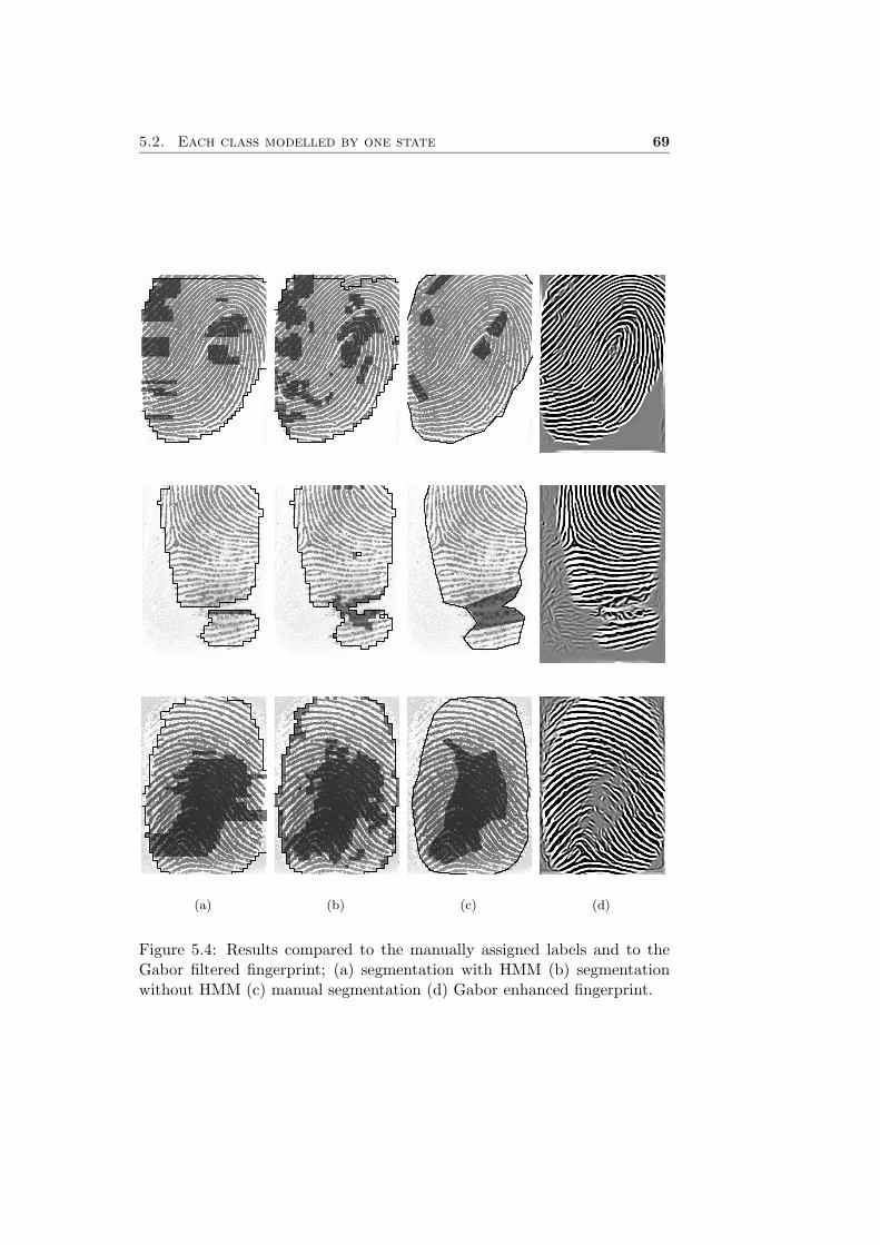
5.2. Each class modelled by one state 69
(a) (b) (c) (d)
Figure 5.4: Results compared to the manually assigned labels and to theGabor filtered fingerprint; (a) segmentation with HMM (b) segmentationwithout HMM (c) manual segmentation (d) Gabor enhanced fingerprint.
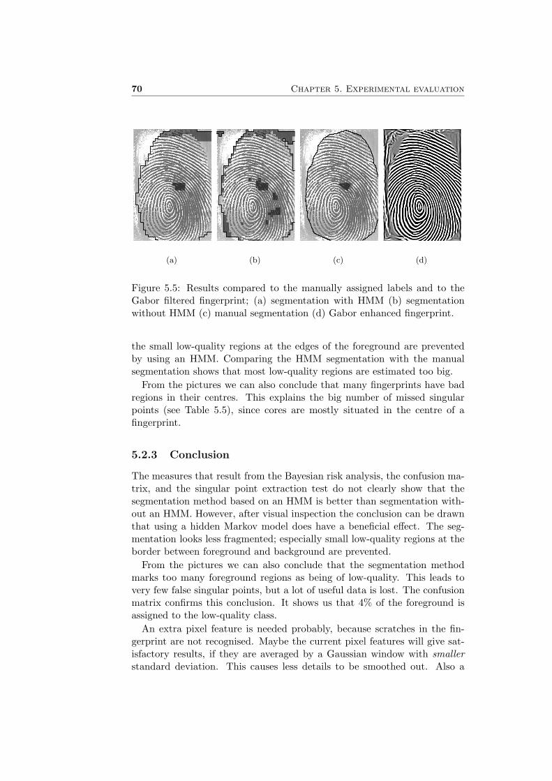
70 Chapter 5. Experimental evaluation
(a) (b) (c) (d)
Figure 5.5: Results compared to the manually assigned labels and to theGabor filtered fingerprint; (a) segmentation with HMM (b) segmentationwithout HMM (c) manual segmentation (d) Gabor enhanced fingerprint.
the small low-quality regions at the edges of the foreground are preventedby using an HMM. Comparing the HMM segmentation with the manualsegmentation shows that most low-quality regions are estimated too big.
From the pictures we can also conclude that many fingerprints have badregions in their centres. This explains the big number of missed singularpoints (see Table 5.5), since cores are mostly situated in the centre of afingerprint.
5.2.3 Conclusion
The measures that result from the Bayesian risk analysis, the confusion ma-trix, and the singular point extraction test do not clearly show that thesegmentation method based on an HMM is better than segmentation with-out an HMM. However, after visual inspection the conclusion can be drawnthat using a hidden Markov model does have a beneficial effect. The seg-mentation looks less fragmented; especially small low-quality regions at theborder between foreground and background are prevented.
From the pictures we can also conclude that the segmentation methodmarks too many foreground regions as being of low-quality. This leads tovery few false singular points, but a lot of useful data is lost. The confusionmatrix confirms this conclusion. It shows us that 4% of the foreground isassigned to the low-quality class.
An extra pixel feature is needed probably, because scratches in the fin-gerprint are not recognised. Maybe the current pixel features will give sat-isfactory results, if they are averaged by a Gaussian window with smallerstandard deviation. This causes less details to be smoothed out. Also a

5.3. Each class modelled by a group of states. 71
decrease of the blocksize may work, although this will increase computationtime.
The usage of a third class besides foreground and background, namelythe low-quality area, has as advantage that the information in these regionsis not totally discarded. Low-quality regions may be reconstructed by in-terpolation of the directional field that lies around. See [23] for possiblereconstruction methods.
5.3 Each class modelled by a group of states.
5.3.1 Description
In the previous section we considered the configuration in which each classis modelled by one state in the HMM. In this section the model is extendedby using more states.
Instead of running again the genetic algorithm we assume that the samepixel features lead to good results as in the simple case. In addition tothese features, the absolute Gabor responses in four orientations are used.Equation (5.1) shows the composition of the observed signal at time t.
Ot =
Local meanStandard deviation
Coherenceabs(Total Gabor)abs(Gabor|θ = 0)
abs(Gabor|θ = π/4)abs(Gabor|θ = π/2)abs(Gabor|θ = 3π/4)
(5.1)
As we suggested in Sections 3.2 and 3.3.5, pixel features have been addedthat provide information about the orientation of the ridge-valley structuresin the foreground.
The four oriented Gabor features imply a 4-state foreground HMM. Theremaining two options, the number of states modelling the background andlow-quality regions, are determined by means of trial and error. The bestresults were obtained with three background states and one state modellinglow-quality regions. Thus, instead of the 3-state HMM that we dealt within Section 5.2, an 8-state HMM is considered now.
The extensions of the HMM topology and the pixel feature vector ap-pear to cause some problems related to the training. As is explained inSection 2.5.2 the sub-HMM of each class is trained separately, using a com-bination of the K -means clustering algorithm and the EM procedure. TheK -means algorithm determines an initial estimate of the HMM parametersand the EM method optimises these parameters by maximising the likeli-hood P (O|λ).
72 Chapter 5. Experimental evaluation
Initialisation
The first problem occurs during initialisation of λF , the parameter set thataccounts for the sub-HMM modelling the foreground.
It is important that the initial values are estimated well, since the EMalgorithm only finds local optima. The foreground sub-HMM has been de-fined consisting of four states. We want that each state corresponds to adirection of the ridge-valley structures. Despite the addition of the fourGabor features, which are highly related to the direction of the lines, theK -means algorithm tends to find other clusters.
To solve this problem we introduce a clustering procedure controlled bythe four pixel features that result from direction oriented Gabor filtering.Four clusters are formed, each corresponding to a state of the sub-HMM. Thefirst cluster consists of all observation vectors with abs(Gabor|θ = 0) havingthe highest value of the four direction oriented Gabor features. The secondone is formed by collecting all observation vectors with abs(Gabor|θ = π/4)being the highest, and so on.
In this way the foreground class is subdivided into four states. The initialparameters of the background and low-quality sub-HMMs are estimated bythe K -means algorithm, as is explained in Section 2.5.2.
Reestimation
After initialisation of the parameter set of a sub-HMM, the EM algorithmis executed to reestimate these parameters. The reestimation functions,written in equations (2.52) to (2.55), are applied iteratively until the valuesconverge. In our case ten iteration steps appeared to be sufficient.
During calculation of the forward and backward variables it is needed toinvert the covariance matrices Σj . Here we encounter a problem becausethe matrix is nearly singular. This means that (nearly) linear dependenciesoccur within the matrix. The total Gabor, the fourth pixel feature, is actu-ally composed of the four direction oriented Gabor features (see Figure 3.12on page 49), so this might explain the problems with singularity.
The solution for this problem is given in [7]. Every EM reestimationstep a diagonal matrix multiplied by a small number has to be added tothe covariance matrix Σj . Some experiments showed that the following

5.3. Each class modelled by a group of states. 73
operation is sufficient to avoid singularity problems.
Σj = Σj + 0.001 ·
0 0 0 0 0 0 0 00 0 0 0 0 0 0 00 0 0 0 0 0 0 00 0 0 1 0 0 0 00 0 0 0 1 0 0 00 0 0 0 0 1 0 00 0 0 0 0 0 1 00 0 0 0 0 0 0 1
(5.2)
5.3.2 Results
The test results with the 8-state configuration that is described in the pre-vious section are presented.
We concluded before that visual inspection is the best method to judgethe results of a segmentation method. In the Figures 5.6, 5.7, and 5.8 the
(a) (b) (c) (d)
Figure 5.6: Segmentation results; (a) segmentation with an 8-state HMM(b) segmentation with a 3-state HMM (c) segmentation without HMM(d) manual segmentation.
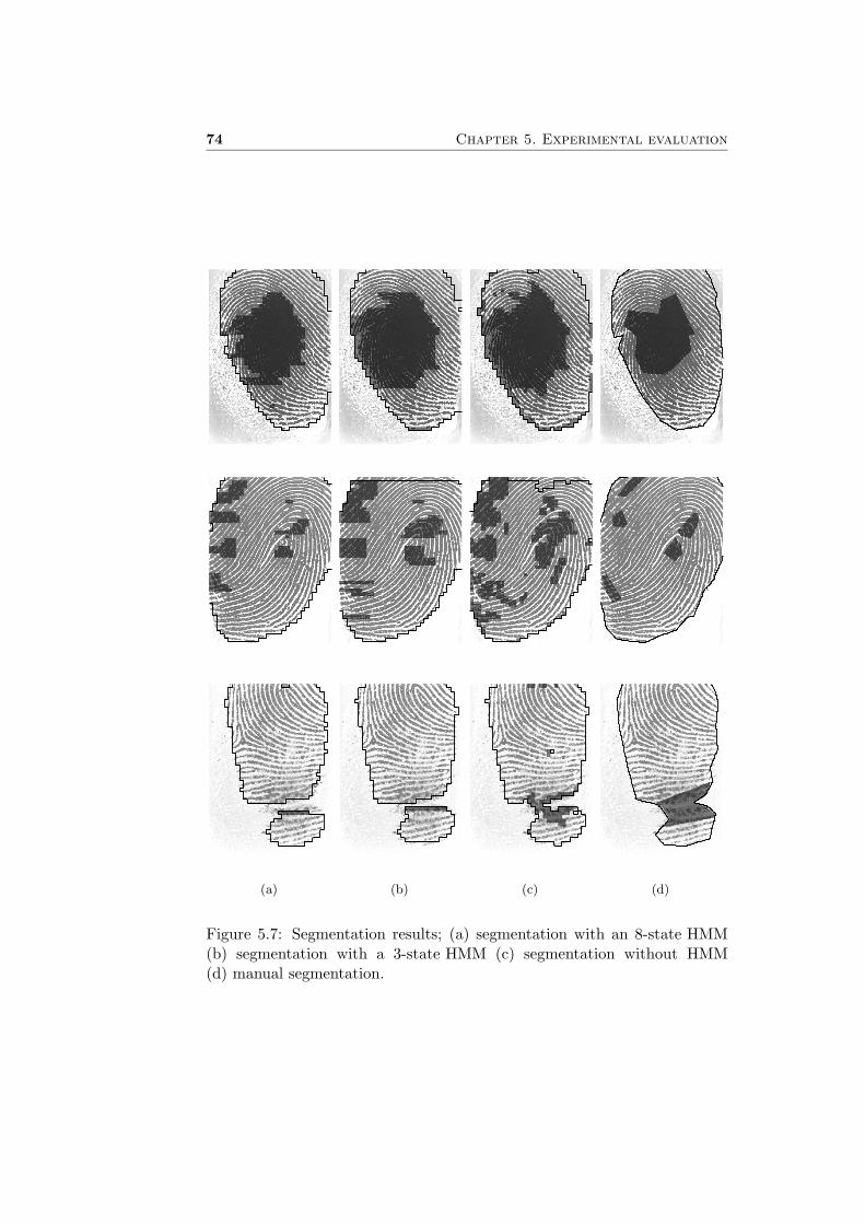
74 Chapter 5. Experimental evaluation
(a) (b) (c) (d)
Figure 5.7: Segmentation results; (a) segmentation with an 8-state HMM(b) segmentation with a 3-state HMM (c) segmentation without HMM(d) manual segmentation.
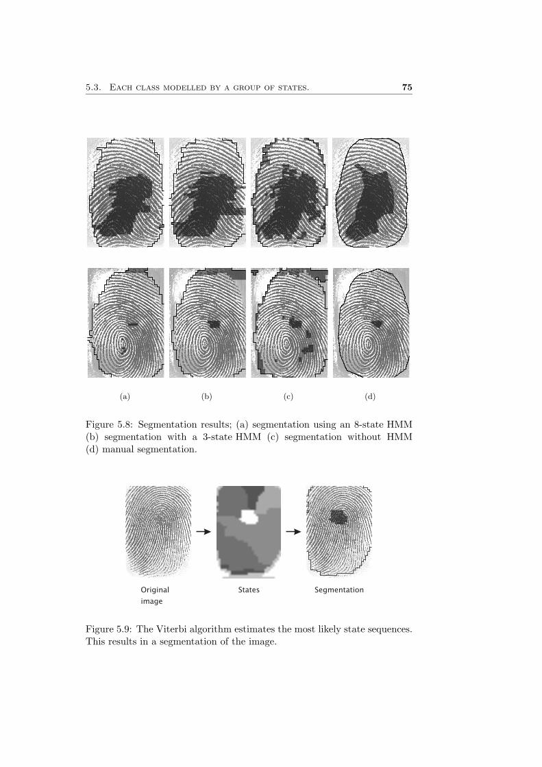
5.3. Each class modelled by a group of states. 75
(a) (b) (c) (d)
Figure 5.8: Segmentation results; (a) segmentation using an 8-state HMM(b) segmentation with a 3-state HMM (c) segmentation without HMM(d) manual segmentation.
Original
image
States Segmentation
Figure 5.9: The Viterbi algorithm estimates the most likely state sequences.This results in a segmentation of the image.
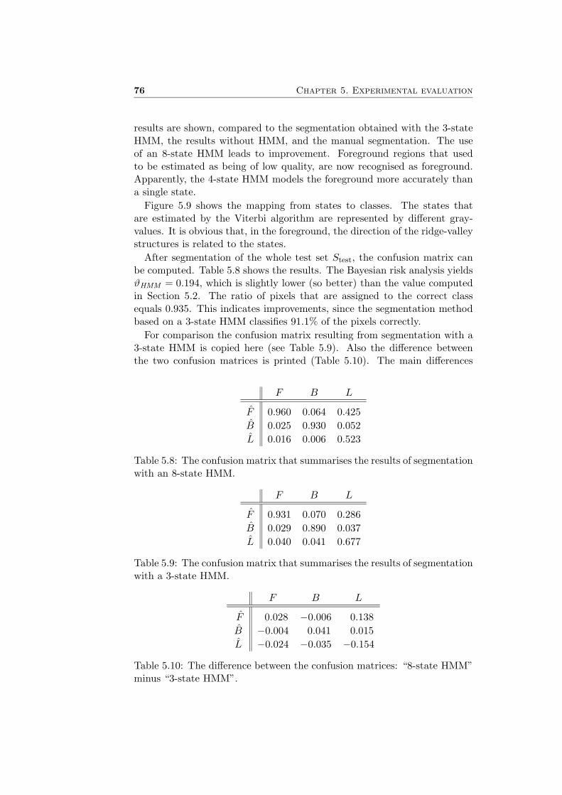
76 Chapter 5. Experimental evaluation
results are shown, compared to the segmentation obtained with the 3-stateHMM, the results without HMM, and the manual segmentation. The useof an 8-state HMM leads to improvement. Foreground regions that usedto be estimated as being of low quality, are now recognised as foreground.Apparently, the 4-state HMM models the foreground more accurately thana single state.
Figure 5.9 shows the mapping from states to classes. The states thatare estimated by the Viterbi algorithm are represented by different gray-values. It is obvious that, in the foreground, the direction of the ridge-valleystructures is related to the states.
After segmentation of the whole test set Stest, the confusion matrix canbe computed. Table 5.8 shows the results. The Bayesian risk analysis yieldsϑHMM = 0.194, which is slightly lower (so better) than the value computedin Section 5.2. The ratio of pixels that are assigned to the correct classequals 0.935. This indicates improvements, since the segmentation methodbased on a 3-state HMM classifies 91.1% of the pixels correctly.
For comparison the confusion matrix resulting from segmentation with a3-state HMM is copied here (see Table 5.9). Also the difference betweenthe two confusion matrices is printed (Table 5.10). The main differences
F B L
F 0.960 0.064 0.425B 0.025 0.930 0.052L 0.016 0.006 0.523
Table 5.8: The confusion matrix that summarises the results of segmentationwith an 8-state HMM.
F B L
F 0.931 0.070 0.286B 0.029 0.890 0.037L 0.040 0.041 0.677
Table 5.9: The confusion matrix that summarises the results of segmentationwith a 3-state HMM.
F B L
F 0.028 −0.006 0.138B −0.004 0.041 0.015L −0.024 −0.035 −0.154
Table 5.10: The difference between the confusion matrices: “8-state HMM”minus “3-state HMM”.
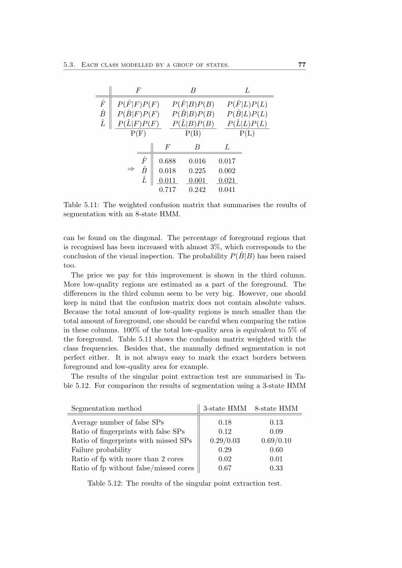
5.3. Each class modelled by a group of states. 77
F B L
F P (F |F )P (F ) P (F |B)P (B) P (F |L)P (L)B P (B|F )P (F ) P (B|B)P (B) P (B|L)P (L)L P (L|F )P (F ) P (L|B)P (B) P (L|L)P (L)
P(F) P(B) P(L)
⇒
F B L
F 0.688 0.016 0.017B 0.018 0.225 0.002L 0.011 0.001 0.021
0.717 0.242 0.041
Table 5.11: The weighted confusion matrix that summarises the results ofsegmentation with an 8-state HMM.
can be found on the diagonal. The percentage of foreground regions thatis recognised has been increased with almost 3%, which corresponds to theconclusion of the visual inspection. The probability P (B|B) has been raisedtoo.
The price we pay for this improvement is shown in the third column.More low-quality regions are estimated as a part of the foreground. Thedifferences in the third column seem to be very big. However, one shouldkeep in mind that the confusion matrix does not contain absolute values.Because the total amount of low-quality regions is much smaller than thetotal amount of foreground, one should be careful when comparing the ratiosin these columns. 100% of the total low-quality area is equivalent to 5% ofthe foreground. Table 5.11 shows the confusion matrix weighted with theclass frequencies. Besides that, the manually defined segmentation is notperfect either. It is not always easy to mark the exact borders betweenforeground and low-quality area for example.
The results of the singular point extraction test are summarised in Ta-ble 5.12. For comparison the results of segmentation using a 3-state HMM
Segmentation method 3-state HMM 8-state HMM
Average number of false SPs 0.18 0.13Ratio of fingerprints with false SPs 0.12 0.09Ratio of fingerprints with missed SPs 0.29/0.03 0.69/0.10Failure probability 0.29 0.60Ratio of fp with more than 2 cores 0.02 0.01Ratio of fp without false/missed cores 0.67 0.33
Table 5.12: The results of the singular point extraction test.
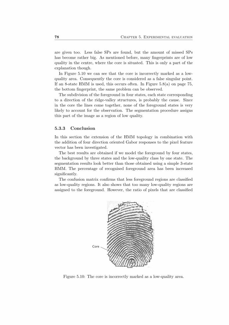
78 Chapter 5. Experimental evaluation
are given too. Less false SPs are found, but the amount of missed SPshas become rather big. As mentioned before, many fingerprints are of lowquality in the centre, where the core is situated. This is only a part of theexplanation though.
In Figure 5.10 we can see that the core is incorrectly marked as a low-quality area. Consequently the core is considered as a false singular point.If an 8-state HMM is used, this occurs often. In Figure 5.8(a) on page 75,the bottom fingerprint, the same problem can be observed.
The subdivision of the foreground in four states, each state correspondingto a direction of the ridge-valley structures, is probably the cause. Sincein the core the lines come together, none of the foreground states is verylikely to account for the observation. The segmentation procedure assignsthis part of the image as a region of low quality.
5.3.3 Conclusion
In this section the extension of the HMM topology in combination withthe addition of four direction oriented Gabor responses to the pixel featurevector has been investigated.
The best results are obtained if we model the foreground by four states,the background by three states and the low-quality class by one state. Thesegmentation results look better than those obtained using a simple 3-stateHMM. The percentage of recognised foreground area has been increasedsignificantly.
The confusion matrix confirms that less foreground regions are classifiedas low-quality regions. It also shows that too many low-quality regions areassigned to the foreground. However, the ratio of pixels that are classified
Core
Figure 5.10: The core is incorrectly marked as a low-quality area.

5.3. Each class modelled by a group of states. 79
correctly indicates improvement, compared to the segmentation method thatuses a 3-state HMM.
The confusion matrix does not show that, with the 8-state HMM, anotherproblem is introduced: very small low-quality regions that are situated ex-actly on the same place as the singular points. This causes many missedsingular points.
The problem might be solved by adding an extra class, which accountsfor singular points. This class can be modelled by one hidden Markov state.
If the pixel feature observations in the singular points have the sameprobability distribution as the observed signal in low-quality regions, thecurrent pixel features do not distinguish between singular points and low-quality regions and the set of pixel features should be extended. Possiblythe coherence that is calculated with a standard deviation σ of 6 pixels leadsto good results, since the core can be distinguished clearly from this feature(see Section 3.3.4).
Instead of adding an extra class, a fifth foreground state may also solvethe problem. In this case, the pixel features have to distinguish even morebetween singular points and low-quality regions, since the singular pointsare not manually labelled anymore.
The 8-state HMM based segmentation method could also be used in com-bination with a simple postprocessing procedure that removes very smalllow-quality regions in the foreground.


Chapter 6
Conclusion andrecommendations
6.1 Conclusion
The usage of a hidden Markov model for fingerprint segmentation has beeninvestigated. First, in Chapter 1, the problems of existing segmentationmethods have been analysed. Second, in Chapter 2 the theory of hiddenMarkov models has been explained. In Chapter 3 we have developed a HMMbased segmentation method and in Chapter 4 a procedure for evaluatingthe performance of the segmentation method is described. Results of theexperimental evaluation have been presented in Chapter 5.
Each row of the fingerprint image is modelled by a hidden Markov process.The classes foreground, background, and low-quality area correspond to oneor more states in the HMM. From the pixel features, which form the outputof the HMM, the underlying states can be estimated. Accordingly, theimage is segmented into foreground, background and low-quality regions.The state transition probabilities (if properly chosen) ensure a classificationthat is consistent with the neighbourhood.
The usage of a third class besides foreground and background, namely thelow-quality area, has as advantage that the information in these regions isnot totally discarded. Low-quality regions may be reconstructed by inter-polation of the directional field that lies around. See also [23] for possiblereconstruction methods.
In Section 1.3 we wrote that four main issues need to be examined:
1. Does the use of hidden Markov models lead to an improved (less frag-mented) segmentation?
2. Which pixel features distinguish clearly between foreground, back-ground and low-quality regions?
3. What is the best topology of the hidden Markov model?
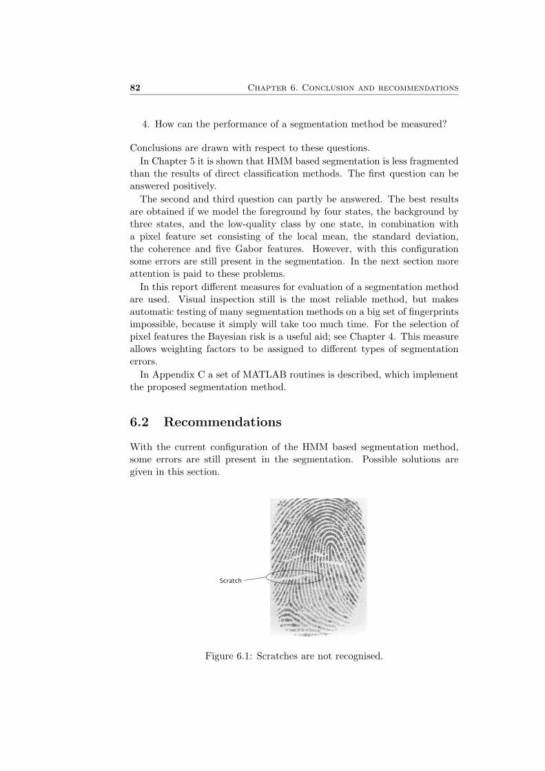
82 Chapter 6. Conclusion and recommendations
4. How can the performance of a segmentation method be measured?
Conclusions are drawn with respect to these questions.In Chapter 5 it is shown that HMM based segmentation is less fragmented
than the results of direct classification methods. The first question can beanswered positively.
The second and third question can partly be answered. The best resultsare obtained if we model the foreground by four states, the background bythree states, and the low-quality class by one state, in combination witha pixel feature set consisting of the local mean, the standard deviation,the coherence and five Gabor features. However, with this configurationsome errors are still present in the segmentation. In the next section moreattention is paid to these problems.
In this report different measures for evaluation of a segmentation methodare used. Visual inspection still is the most reliable method, but makesautomatic testing of many segmentation methods on a big set of fingerprintsimpossible, because it simply will take too much time. For the selection ofpixel features the Bayesian risk is a useful aid; see Chapter 4. This measureallows weighting factors to be assigned to different types of segmentationerrors.
In Appendix C a set of MATLAB routines is described, which implementthe proposed segmentation method.
6.2 Recommendations
With the current configuration of the HMM based segmentation method,some errors are still present in the segmentation. Possible solutions aregiven in this section.
Scratch
Figure 6.1: Scratches are not recognised.

6.2. Recommendations 83
Thin scratches in the fingerprint image (see Figure 6.1) form the firstproblem. The scratches were labelled as low-quality regions, but the auto-matic segmentation considers them as foreground. The problem is caused bythe choice of pixel features, because none of the investigated segmentationmethods recognises scratches as low-quality regions. To recognise them aslow-quality regions, a pixel feature needs to be added that clearly reflectsthese scratches. Maybe the current pixel features will give satisfactory re-sults, if they are averaged by a Gaussian window with smaller standarddeviation. This causes less details to be smoothed out. Also a decrease ofthe blocksize may work, although this will increase computation time.
In Figure 6.2 the second problem is observed. We can see that the coreis incorrectly marked as a low-quality area. Consequently the core is con-sidered as a false singular point. The subdivision of the foreground in fourstates, each state corresponding to a direction of the ridge-valley structures,is probably the cause. Since in the core the lines come together, none ofthe foreground states is very likely to account for the observation. Thesegmentation procedure assigns this part of the image as a region of lowquality.
The problem might be solved by adding an extra class, which accountsfor singular points. This class can be modelled by one hidden Markov state.
If the pixel feature observations in the singular points have the sameprobability distribution as the observed signal in low-quality regions, thecurrent pixel features do not distinguish between singular points and low-quality regions and the set of pixel features should be extended. Possiblythe coherence that is calculated with a standard deviation σ of 6 pixels leadsto good results, since the core can be distinguished clearly from this feature(see Section 3.3.4).
Core
Figure 6.2: The core is incorrectly marked as a low-quality area.
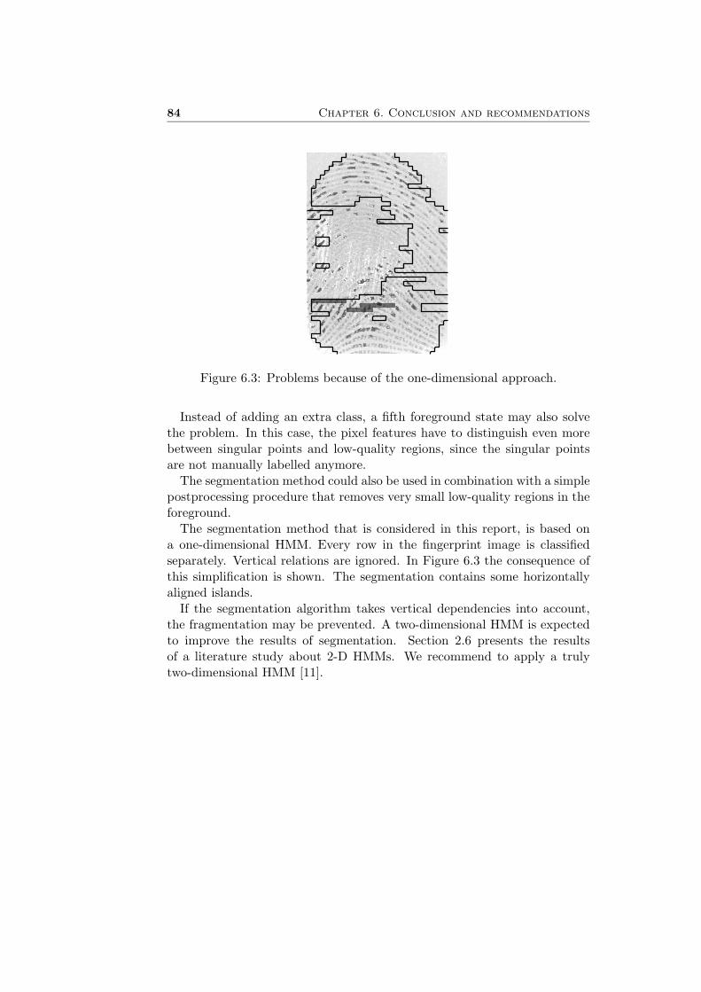
84 Chapter 6. Conclusion and recommendations
Figure 6.3: Problems because of the one-dimensional approach.
Instead of adding an extra class, a fifth foreground state may also solvethe problem. In this case, the pixel features have to distinguish even morebetween singular points and low-quality regions, since the singular pointsare not manually labelled anymore.
The segmentation method could also be used in combination with a simplepostprocessing procedure that removes very small low-quality regions in theforeground.
The segmentation method that is considered in this report, is based ona one-dimensional HMM. Every row in the fingerprint image is classifiedseparately. Vertical relations are ignored. In Figure 6.3 the consequence ofthis simplification is shown. The segmentation contains some horizontallyaligned islands.
If the segmentation algorithm takes vertical dependencies into account,the fragmentation may be prevented. A two-dimensional HMM is expectedto improve the results of segmentation. Section 2.6 presents the resultsof a literature study about 2-D HMMs. We recommend to apply a trulytwo-dimensional HMM [11].

Acknowledgements
This Master of Science thesis has been written for the laboratory of Signalsand Systems, which is part of the department of Electrical Engineering,University of Twente.
The author would like to thank Asker Bazen, Bart Koopman, Kees Slump,and Raymond Veldhuis for excellent help.

Appendix A
The Viterbi algorithm
In this appendix the derivation of the recursive equation (2.17) (Section 2.3)is described. This formula plays an important role in the Viterbi algorithm,which is used for finding the state sequence that most likely accounts for anobserved output signal of an HMM.
The Viterbi algorithm finds the state sequence Q? = Q?1 . . . Q?
t . . . Q?T that
maximises the probability P (Q, O|λ).
Q? = argmaxQ
P (Q, O|λ) (A.1)
In Section 2.3 we defined the quantity δ:
δt(i) = maxQ1,Q2,...,Qt−1
P (Q1Q2 . . . Qt = i, O1O2 . . . Ot|λ) (A.2)
This variable is in such way defined that
maxQ
[P (Q, O|λ)] = maxi
δT (i) (A.3)
and thus provides a way to find Q?, as is explained in Section 2.3. Cal-culation of δt(i) for all t and i is achieved by means of the recursive equa-tion (2.17):
δt+1(j) = maxi
[δt(i)aij ] · bj(Ot+1) (A.4)
Derivation of this expression is described in this appendix.Using the general equation P (AB) = P (A|B) · P (B) the expression for δ
is transformed:
δt(j) = maxQ1,...,Qt−1
P (Q1 . . . Qt = j, O1 . . . Ot|λ)
= maxQ1,...,Qt−1
[P (Qt = j, Ot|Q1 . . . Qt−1, O1 . . . Ot−1, λ)
·P (Q1 . . . Qt−1, O1 . . . Ot−1|λ)]
(A.5)

88 Appendix A. The Viterbi algorithm
In a first order hidden Markov model the observations O1 . . . Ot−1 and thestates Q1 . . . Qt−2 do not influence Qt and Ot. Only the predecessor stateQt−1 is important.
δt(j) = maxQ1,...,Qt−1
[P (Qt = j, Ot|Q1 . . . Qt−1, O1 . . . Ot−1, λ)
·P (Q1 . . . Qt−1, O1 . . . Ot−1|λ)]
= maxQ1,...,Qt−1
[P (Qt = j, Ot|Qt−1, λ)
·P (Q1 . . . Qt−1, O1 . . . Ot−1|λ)]
(A.6)
This can be transformed to:
δt(j) = maxQt−1
[P (Qt = j, Ot|Qt−1, λ)
· maxQ1,...,Qt−2
P (Q1 . . . Qt−1, O1 . . . Ot−1|λ)]
(A.7)
The expression P (Qt = j, Ot|Qt−1, λ) is expanded using P (AB) = P (A|B) ·P (B):
δt(j) = maxQt−1
[P (Ot|Qt = j, Qt−1, λ) · P (Qt = j|Qt−1, λ)
· maxQ1,...,Qt−2
P (Q1 . . . Qt−1, O1 . . . Ot−1|λ)]
(A.8)
Since Ot does not depend on Qt−1, this turns into:
δt(j) = maxQt−1
[P (Ot|Qt = j, λ) · P (Qt = j|Qt−1, λ)
· maxQ1,...,Qt−2
P (Q1 . . . Qt−1, O1 . . . Ot−1|λ)]
(A.9)
Now Qt−1 = i is substituted,
δt(j) = maxi
[P (Ot|Qt = j, λ) · P (Qt = j|Qt−1 = i, λ)
· maxQ1,...,Qt−2
P (Q1 . . . Qt−1 = i, O1 . . . Ot−1|λ)]
(A.10)
which allows us to recognise the factors aij , bj(Ot) and δt−1(i):
δt(j) = maxi
[bj(Ot) · aij · δt−1(i)] (A.11)
Since bj(Ot) does not depend on i this factor can be moved outside thebrackets:
δt(j) = maxi
[aij · δt−1(i)] · bj(Ot) (A.12)
Substituting t + 1 for t yields equation (A.4), which was aimed at.

Appendix B
The EM algorithm
In this appendix the EM reestimation functions that are mentioned in Sec-tion 2.5.2 are derived. More information about the EM algorithm can befound in [16], [20], and in [21]. For HMMs with mixtures of Gaussian dis-tributions (M > 1) [8] is a good information source.
We want to determine the hidden Markov process that most likely ac-counts for a certain observed signal O. This means that we have to find theHMM parameter set λ that maximises P (O|λ). Since the state sequence Qis hidden, our data is called “incomplete”. For these kind of optimisationproblems the expectation-maximisation method can be used. The proce-dure, which is iteratively executed, consists of two steps.
• Expectation (E):
Q(λ|λ[k]) = E[log P (O, Q|λ)|O, λ[k]
](B.1)
where λ[k] is the estimate of the parameters at the k-th iteration.
• Maximisation (M):
λ[k+1] = argmaxλ
Q(λ|λ[k]) (B.2)
where λ[k+1] is the reestimated parameter set.
In every M-step Q(λ|λ[k]) is maximised. Actually we would like to max-imise P (O, Q|λ), but Q is unknown (hidden), so we need to maximise theexpectancy of P (O, Q|λ) given the observed signal O and the current pa-rameter estimate λ[k]. In [1] it has been proven that:
Q(λ[k+1]|λ[k]) ≥ Q(λ[k]|λ[k]) ⇒ P (O|λ[k+1]) ≥ P (O|λ[k]) (B.3)
This iterative procedure converges to the limiting point λ[k+1] = λ[k]. A(local) maximum of P (O|λ) has been reached then.
The expectation and maximisation steps are described in detail here.

90 Appendix B. The EM algorithm
E-step
The expression for Q is recalled:
Q(λ|λ[k]) = E[log P (O, Q|λ)|O, λ[k]
](B.4)
The definition of expectancy is used to obtain:
Q(λ|λ[k]) =∑Q
P (Q|O, λ[k]) log P (O, Q|λ) (B.5)
This can be transformed to:
Q(λ|λ[k]) =1
P (O|λ[k])
∑Q
P (Q, O|λ[k]) log P (O|Q, λ)P (Q|λ) (B.6)
The log-likelihoods P (O|Q, λ) and P (Q|λ) are given by:
P (O|Q, λ) =T∏
t=1
P (Ot|Qt, λ)
=T∏
t=1
bQt(Ot) (B.7)
P (Q|λ) = πQ1
T∏t=2
aQt−1Qt (B.8)
Substitution of these equations in (B.6) leads to equation (B.9):
Q(λ|λ[k]) =1
P (O|λ[k])
∑Q
P (Q, O|λ[k])
·[
T∑t=1
log bQt(Ot) + log πQ1 +T∑
t=2
log aQt−1Qt
](B.9)
In the next step, this function will be maximised.
M-step
We would like to find the parameters π, A, c, µ and Σ that maximiseQ(λ|λ[k]):
λ[k+1] = argmaxλ
Q(λ|λ[k]) (B.10)
For aij , an element of the transition matrix A, the optimisation will beexplained. This ultimately will lead to the reestimation function that iswritten in Section 2.5.2.
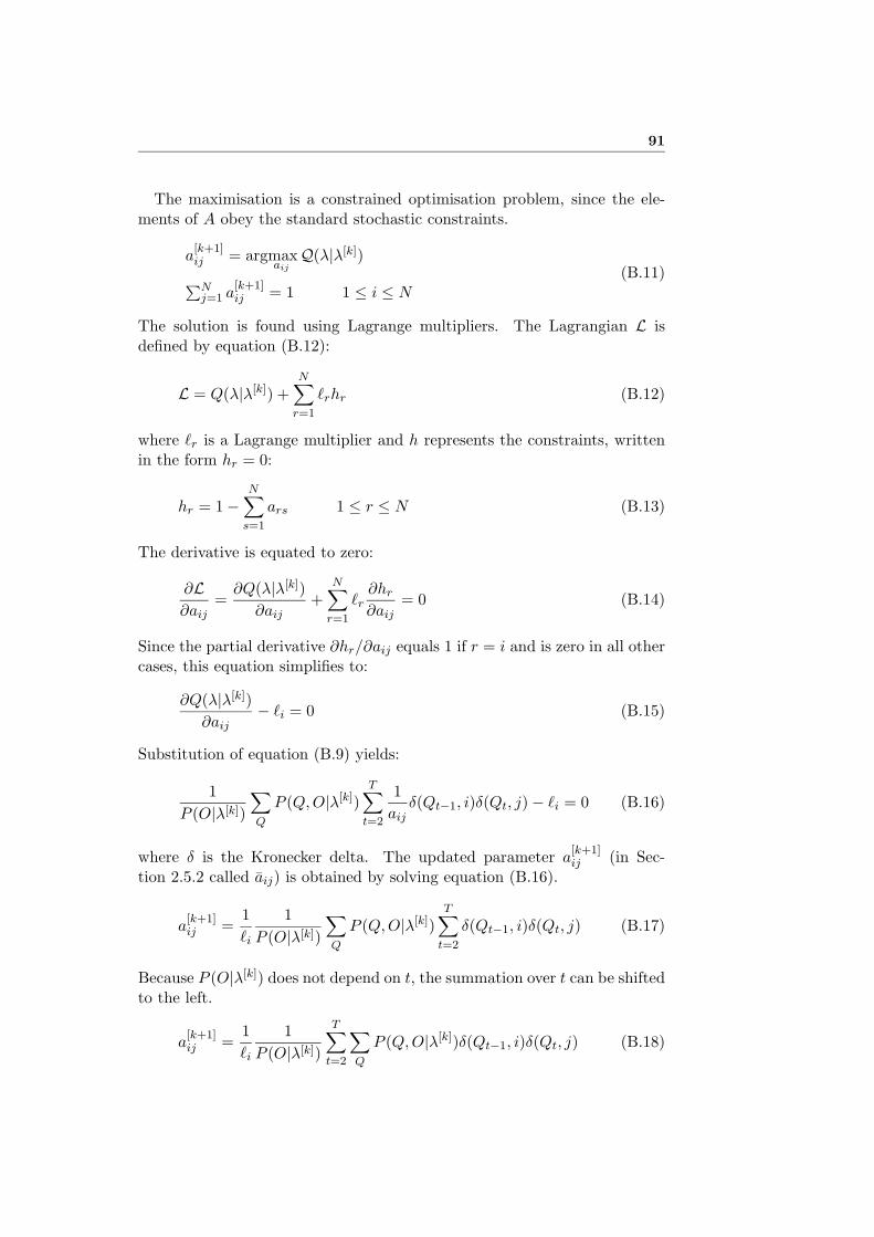
91
The maximisation is a constrained optimisation problem, since the ele-ments of A obey the standard stochastic constraints.
a[k+1]ij = argmaxQ(λ|λ[k])
aij∑Nj=1 a
[k+1]ij = 1 1 ≤ i ≤ N
(B.11)
The solution is found using Lagrange multipliers. The Lagrangian L isdefined by equation (B.12):
L = Q(λ|λ[k]) +N∑
r=1
`rhr (B.12)
where `r is a Lagrange multiplier and h represents the constraints, writtenin the form hr = 0:
hr = 1 −N∑
s=1
ars 1 ≤ r ≤ N (B.13)
The derivative is equated to zero:
∂L∂aij
=∂Q(λ|λ[k])
∂aij+
N∑r=1
`r∂hr
∂aij= 0 (B.14)
Since the partial derivative ∂hr/∂aij equals 1 if r = i and is zero in all othercases, this equation simplifies to:
∂Q(λ|λ[k])∂aij
− `i = 0 (B.15)
Substitution of equation (B.9) yields:
1P (O|λ[k])
∑Q
P (Q, O|λ[k])T∑
t=2
1aij
δ(Qt−1, i)δ(Qt, j) − `i = 0 (B.16)
where δ is the Kronecker delta. The updated parameter a[k+1]ij (in Sec-
tion 2.5.2 called aij) is obtained by solving equation (B.16).
a[k+1]ij =
1`i
1P (O|λ[k])
∑Q
P (Q, O|λ[k])T∑
t=2
δ(Qt−1, i)δ(Qt, j) (B.17)
Because P (O|λ[k]) does not depend on t, the summation over t can be shiftedto the left.
a[k+1]ij =
1`i
1P (O|λ[k])
T∑t=2
∑Q
P (Q, O|λ[k])δ(Qt−1, i)δ(Qt, j) (B.18)

92 Appendix B. The EM algorithm
This can also be written as:
a[k+1]ij =
1`i
1P (O|λ[k])
T∑t=2
∑{Q|Qt−1=i,Qt=j}
P (Q, O|λ[k]) (B.19)
The Langrange multiplier `i is chosen to normalise a[k+1]ij . In this way, we
ensure that A[k+1] obeys the standard stochastic constraints.
`i =1
P (O|λ[k])
N∑j=1
T∑t=2
∑{Q|Qt−1=i,Qt=j}
P (Q, O|λ[k])
=1
P (O|λ[k])
T∑t=2
∑{Q|Qt−1=i}
P (Q, O|λ[k]) (B.20)
The likelihoods can be expressed in the forward and backward variables (seeSection 2.4):
a[k+1]ij =
∑Tt=2
∑{Q|Qt−1=i,Qt=j} P (Q, O|λ[k])∑T
t=2
∑{Q|Qt−1=i} P (Q, O|λ[k])
=∑T
t=2 αt−1(i)aijbj(Ot)βt(j)∑Tt=2 αt−1(i)βt−1(i)
(B.21)
which equals the reestimation expression (2.53) that is stated in Section 2.5.2.For the other HMM parameters the derivation is comparable.

Appendix C
MATLAB functions
A set of MATLAB routines has been written for HMM based segmentation.The functions are described in this appendix.
The routines implement the segmentation method that is tested in Sec-tion 5.3. In this configuration the foreground is modelled by four HMMstates, the background by three states, and the low-quality class by onestate. The pixel feature vector consists of the local mean, the standarddeviation, the coherence, the absolute total Gabor response and the fouroriented Gabor features.
The following list contains the function headings and explains shortly howto use them. Type help <function> for more detailed information abouta function.
• [segmask, segmaskB, states, statesB]= HMMseg(fp, labda, features);
This function segments a fingerprint. The input is a gray-value fin-gerprint image fp, the HMM parameter set labda (λ), and an arrayfeatures that contains the pixel features of the fingerprint image. Ifthe features parameter is omitted, the function itself will computethe pixel features of the fingerprint image. The output is formed byfour arrays, which contain the segmentation results in different for-mats.
• dispHMMseg(fp, segmask);
This function displays a fingerprint and its segmentation, which hasbeen obtained by HMMseg.
• [features] = HMMfeatures(fp);
This function can be used to calculate the pixel features of a fingerprintfp. The output variable, features, serves as an input for the HMMsegfunction.

94 Appendix C. MATLAB functions
• [labda] = LoadLabda(filename);
This function loads the HMM parameter set λ from a file filenameinto the workspace. The output is a structure consisting of five fields:
labda.prior : the initial state probability vector (π)labda.transmat : the transition matrix (A)labda.mixmat : the weighting factors (c) of the Gaussian density
functionslabda.mu : the means (µ) of the Gaussian density functionslabda.Sigma : the covariance matrices (Σ) of the Gaussian den-
sity functions
The labda variable is needed for executing HMMseg. For each finger-print database a new parameter set has to be computed. The pro-gram HMMTraining can be used for this task. A standard parameterset StandardLabda.mat is included, which is optimised for database2 of the Fingerprint Verification Competition (FVC2000) [12]. Thisset will in general not give satisfactory segmentation results on otherfingerprint databases.
• HMMTraining;
With this program fingerprints can be manually segmented. Based onthese labels, the automatic segmentation method is trained.
A graphic user interface is launched when the program is executed,see Figure C.1. After starting the program, first define the folder inwhich the fingerprints are stored (‘Fingerprint folder’) and the ‘Savefolder’, in which you want to save the manual segmentation data(manseg *.mat), the pixel feature data (features *.mat), and thetraining results (labda.mat).
Then the manual segmentation can be started.
– Pick a fingerprint image in the ‘Fingerprint folder’. The finger-print will be shown.
– Press the ‘Draw foreground/background border’ button. Now aline can be drawn, composed of vertices that are defined by left-clicks. A right-click places a final vertex.
– Defining low-quality regions goes the same way.
– When a mistake has been made, press the ‘Clear’ button.
– Checking the Gabor enhancement checkbox yields an image thatmay be helpful for manual segmentation. The picture showswhere probably mistakes will be made in the further fingerprintrecognition process (see also Section 4.2)
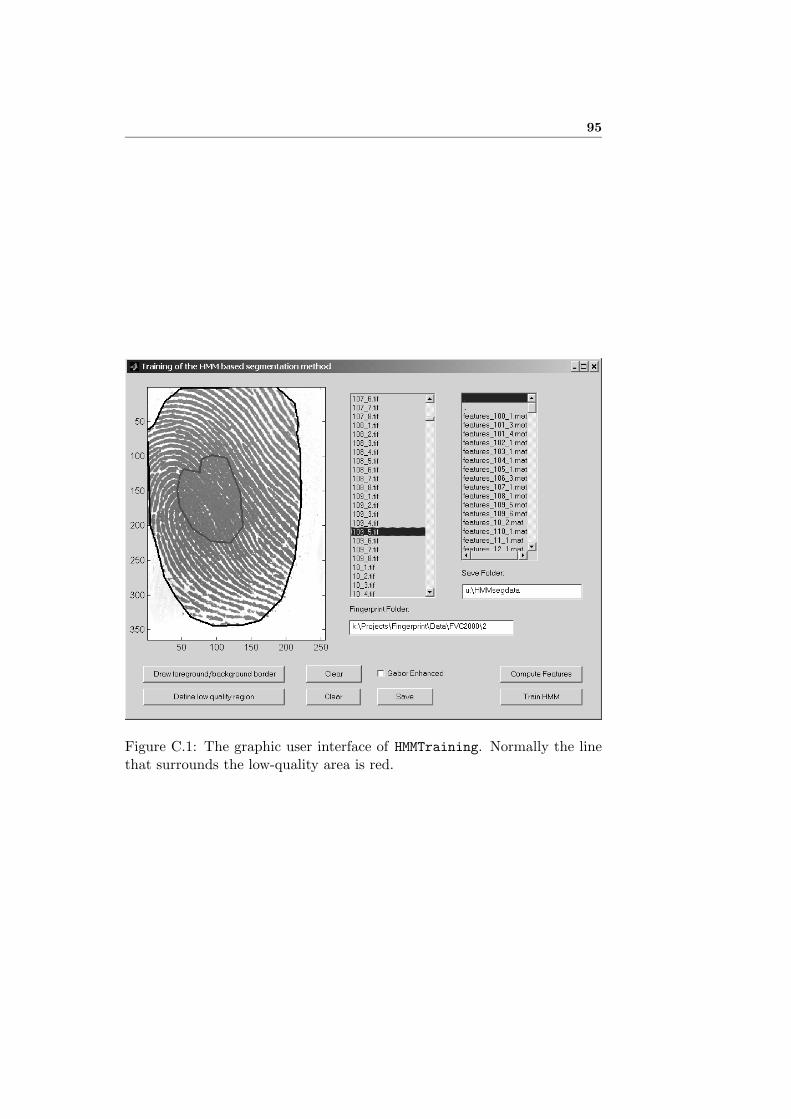
95
Figure C.1: The graphic user interface of HMMTraining. Normally the linethat surrounds the low-quality area is red.

96 Appendix C. MATLAB functions
The manual segmentation can be saved by pressing the ‘Save’ but-ton. The segmentation data will be saved as manseg <FP-name>.mat,where <FP-name> represents the name of the fingerprint image.
When the training set is big enough the training can be started.
– Press ‘Compute Features’ to compute the pixel features of allmanually segmented fingerprints. The pixel features of a finger-print are saved as features <FP-name>.mat. If this file alreadyexists, the pixel features are not calculated again.
– Press ‘Train HMM’ to start training. This can take a while, so bepatient. The results are stored in the ‘Save folder’ as labda.mat.
The file labda.mat is needed for segmentation of a fingerprint usingHMMseg, and can be loaded with the function LoadLabda.
The following example MATLAB code shows how to segment a fingerprint:
fp = ReadFP( ’c:\fingerprints\14_3.tif’ );
features = HMMfeatures( fp );
labda = LoadLabda( ’c:\HMMsegTrainingData\labda.mat’ );
segmask = HMMseg( fp, labda, features );
dispHMMseg( fp, segmask );
which results in the fingerprint shown in Figure C.2.
Figure C.2: The result of fingerprint segmentation. The black line representsthe border between the foreground and the background. Low-quality regionsare displayed darker.

Appendix D
Paper ProRISC2002
The following paper has been written for the ProRISC2002 conference(http://www.stw.nl/prorisc).
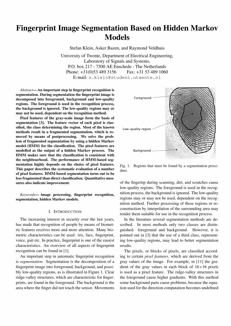
Fingerprint Image Segmentation Based on Hidden Markov
Models
Stefan Klein, Asker Bazen, and Raymond Veldhuis
University of Twente, Department of Electrical Engineering,
Laboratory of Signals and Systems,
P.O. box 217 - 7500 AE Enschede - The Netherlands
Phone: +31(0)53 489 3156 Fax: +31 53 489 1060
E-mail: [email protected]
Abstract—An important step in fingerprint recognition is
segmentation. During segmentation the fingerprint image is
decomposed into foreground, background and low-quality
regions. The foreground is used in the recognition process,
the background is ignored. The low-quality regions may or
may not be used, dependent on the recognition method.
Pixel features of the gray-scale image form the basis of
segmentation [3]. The feature vector of each pixel is clas-
sified, the class determining the region. Most of the known
methods result in a fragmented segmentation, which is re-
moved by means of postprocessing. We solve the prob-
lem of fragmented segmentation by using a hidden Markov
model (HMM) for the classification. The pixel features are
modelled as the output of a hidden Markov process. The
HMM makes sure that the classification is consistent with
the neighbourhood. The performance of HMM-based seg-
mentation highly depends on the choice of pixel features.
This paper describes the systematic evaluation of a number
of pixel features. HMM-based segmentation turns out to be
less fragmented than direct classification. Quantitative mea-
sures also indicate improvement.
Keywords— image processing, fingerprint recognition,
segmentation, hidden Markov models.
I. INTRODUCTION
The increasing interest in security over the last years,
has made that recognition of people by means of biomet-
ric features receives more and more attention. Many bio-
metric characteristics can be used: iris, face, fingerprint,
voice, gait etc. In practice, fingerprint is one of the easiest
characteristics. An overview of all aspects of fingerprint
recognition can be found in [1].
An important step in automatic fingerprint recognition
is segmentation. Segmentation is the decomposition of a
fingerprint image into foreground, background, and possi-
bly low-quality regions, as is illustrated in Figure 1. Clear
ridge-valley structures, which are characteristic for finger-
prints, are found in the foreground. The background is the
area where the finger did not touch the sensor. Movements
Fig. 1. Regions that must be found by a segmentation proce-
dure.
of the fingertip during scanning, dirt, and scratches cause
low-quality regions. The foreground is used in the recog-
nition process, the background is ignored. The low-quality
regions may or may not be used, dependent on the recog-
nition method. Further processing of these regions or re-
construction by interpolation of the surrounding area may
render them suitable for use in the recognition process.
In the literature several segmentation methods are de-
scribed. In most methods only two classes are distin-
guished: foreground and background. However, it is
pointed out in [3] that the use of a third class, represent-
ing low-quality regions, may lead to better segmentation
results.
The pixels, or blocks of pixels, are classified accord-
ing to certain pixel features, which are derived from the
gray values of the image. For example, in [11] the gra-
dient of the gray values in each block of 16×16 pixels
is used as a pixel feature. The ridge-valley structures in
the foreground cause higher gradients. With this method
some background parts cause problems, because the equa-
tion used for the direction computation becomes undefined

(a) Before morphology (b) After morphology
Fig. 2. Result of a segmentation method that requires postpro-
cessing.
when the input image has perfectly uniform regions. To
solve this problem the method described in [10] uses the
gray-scale variance of the block in addition to the gradient.
A region whose gray-scale variance is lower than a certain
threshold is marked as background. In [14] the gray scale
variance orthogonal to the orientation of the ridges is used
to classify each 16×16 block. In [2] the coherence is cal-
culated for each pixel. The coherence measures how well
the gradients are pointing in the same direction and yields
high values in the foreground. In [6] the output of a set
of Gabor filters is used, which smooth the image along the
direction of the line structures. A linear combination of
three features is proposed in [3]. This paper describes the
systematic evaluation of a number of pixel features.
While classifying a block, none of the aforementioned
methods take the classes of neighbouring blocks into ac-
count. This may lead to a fragmented segmentation, as
shown in Figure 2(a). Currently, this problem is mostly
solved by postprocessing the image, for example using
morphology [5]; see Figure 2(b).
In this paper a segmentation method is presented, based
on pixel features, that also aims at a classification con-
sistent with the neighbouring blocks. The pixel features
are modelled as the output of a hidden Markov process.
Hidden Markov models, which are widely used in speech
recognition [13], assume a set of states, determining the
statistical properties of the output. Transitions between
states take place according to predefined transition prob-
abilities, but the state of the process is hidden for the ob-
server. The most likely state sequence can be estimated by
maximising the probability of the state sequence given the
observed signal and the transition probabilities.
Fig. 3. Example of a hidden Markov model .
If we model the fingerprint in such way that the fore-
ground, background, and low-quality regions correspond
to states (or groups of states) in a hidden Markov process,
then the state transition probabilities ensure an estimation
that is consistent with the neighbourhood.
The parameters of the hidden Markov model are trained
on a set of manually labelled fingerprints, in which fore-
ground, background, and low-quality regions are marked.
Section II describes the application of a hidden Markov
model on fingerprint segmentation and the results are pre-
sented in Section III. The paper ends with conclusions and
recommendations.
II. SEGMENTATION USING AN HMM
A. The hidden Markov model
In this section the general hidden Markov model is ex-
plained. The next section deals with application of this
model to the fingerprint segmentation problem.
A hidden Markov model (HMM) is statistical signal
model. Figure 3 shows an example of an HMM. The sys-
tem can be in three states, q1, q2, and q3, which are hidden
for the observer. A sequence of states that are visited dur-
ing a process is notated as:
Q = Q1Q2 . . . Q t . . . QT (1)
The probability that state i is the initial state Q1, is called
the initial state probability πi . The coefficients ai j form a
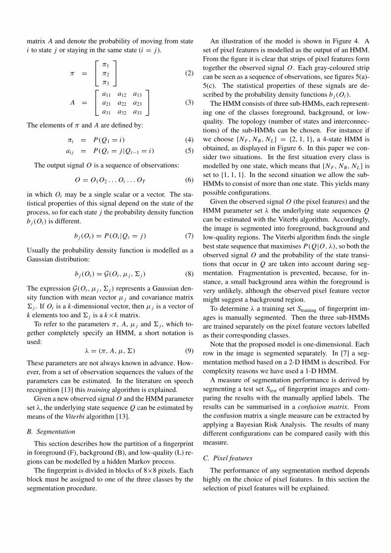
matrix A and denote the probability of moving from state
i to state j or staying in the same state (i = j).
π =
π1
π2
π3
(2)
A =
a11 a12 a13
a21 a22 a23
a31 a32 a33
(3)
The elements of π and A are defined by:
πi = P(Q1 = i) (4)
ai j = P(Q t = j |Qt−1 = i) (5)
The output signal O is a sequence of observations:
O = O1O2 . . . Ot . . . OT (6)
in which Ot may be a single scalar or a vector. The sta-
tistical properties of this signal depend on the state of the
process, so for each state j the probability density function
b j (Ot) is different.
b j (Ot) = P(Ot |Qt = j) (7)
Usually the probability density function is modelled as a
Gaussian distribution:
b j (Ot) = G(Ot , µ j , 6 j ) (8)
The expression G(Ot , µ j , 6 j ) represents a Gaussian den-
sity function with mean vector µ j and covariance matrix
6 j . If Ot is a k-dimensional vector, then µ j is a vector of
k elements too and 6 j is a k×k matrix.
To refer to the parameters π , A, µ j and 6 j , which to-
gether completely specify an HMM, a short notation is
used:
λ = (π, A, µ, 6) (9)
These parameters are not always known in advance. How-
ever, from a set of observation sequences the values of the
parameters can be estimated. In the literature on speech
recognition [13] this training algorithm is explained.
Given a new observed signal O and the HMM parameter
set λ, the underlying state sequence Q can be estimated by
means of the Viterbi algorithm [13].
B. Segmentation
This section describes how the partition of a fingerprint
in foreground (F), background (B), and low-quality (L) re-
gions can be modelled by a hidden Markov process.
The fingerprint is divided in blocks of 8×8 pixels. Each
block must be assigned to one of the three classes by the
segmentation procedure.
An illustration of the model is shown in Figure 4. A
set of pixel features is modelled as the output of an HMM.
From the figure it is clear that strips of pixel features form
together the observed signal O . Each gray-coloured strip
can be seen as a sequence of observations, see figures 5(a)-
5(c). The statistical properties of these signals are de-
scribed by the probability density functions b j (Ot).
The HMM consists of three sub-HMMs, each represent-
ing one of the classes foreground, background, or low-
quality. The topology (number of states and interconnec-
tions) of the sub-HMMs can be chosen. For instance if
we choose {NF , NB, NL} = {2, 1, 1}, a 4-state HMM is
obtained, as displayed in Figure 6. In this paper we con-
sider two situations. In the first situation every class is
modelled by one state, which means that {NF , NB, NL} is
set to {1, 1, 1}. In the second situation we allow the sub-
HMMs to consist of more than one state. This yields many
possible configurations.
Given the observed signal O (the pixel features) and the
HMM parameter set λ the underlying state sequences Q
can be estimated with the Viterbi algorithm. Accordingly,
the image is segmented into foreground, background and
low-quality regions. The Viterbi algorithm finds the single
best state sequence that maximises P(Q|O, λ), so both the
observed signal O and the probability of the state transi-
tions that occur in Q are taken into account during seg-
mentation. Fragmentation is prevented, because, for in-
stance, a small background area within the foreground is
very unlikely, although the observed pixel feature vector
might suggest a background region.
To determine λ a training set Straining of fingerprint im-
ages is manually segmented. Then the three sub-HMMs
are trained separately on the pixel feature vectors labelled
as their corresponding classes.
Note that the proposed model is one-dimensional. Each
row in the image is segmented separately. In [7] a seg-
mentation method based on a 2-D HMM is described. For
complexity reasons we have used a 1-D HMM.
A measure of segmentation performance is derived by
segmenting a test set Stest of fingerprint images and com-
paring the results with the manually applied labels. The
results can be summarised in a confusion matrix. From
the confusion matrix a single measure can be extracted by
applying a Bayesian Risk Analysis. The results of many
different configurations can be compared easily with this
measure.
C. Pixel features
The performance of any segmentation method depends
highly on the choice of pixel features. In this section the
selection of pixel features will be explained.
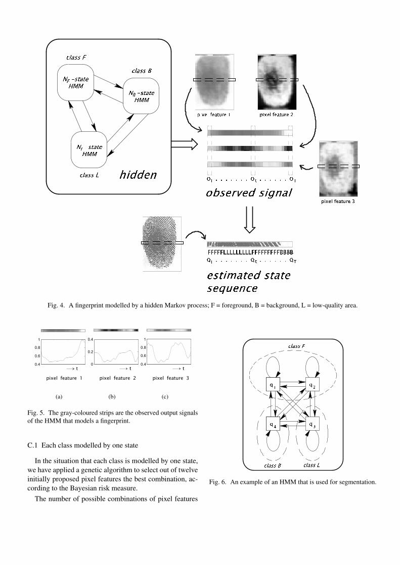
Fig. 4. A fingerprint modelled by a hidden Markov process; F = foreground, B = background, L = low-quality area.
0.4
0.6
0.8
1
pixel feature 1
t
(a)
0
0.2
0.4
pixel feature 2
t
(b)
0.4
0.6
0.8
1
pixel feature 3
t
(c)
Fig. 5. The gray-coloured strips are the observed output signals
of the HMM that models a fingerprint.
C.1 Each class modelled by one state
In the situation that each class is modelled by one state,
we have applied a genetic algorithm to select out of twelve
initially proposed pixel features the best combination, ac-
cording to the Bayesian risk measure.
The number of possible combinations of pixel features
Fig. 6. An example of an HMM that is used for segmentation.

(a) Original (b) Re(Gabor) (c) Abs(Gabor) (d) Local mean (e) Standard devi-
ation
(f) Coherence
Fig. 7. Pixel features for two fingerprints; (a) the original fingerprints (b) real part of Gabor response (c) absolute values of Gabor
response (d) local mean (e) standard deviation (f) coherence. Black pixels represent low values, white pixels high values. The gray
scales of (a)-(f) can not be compared.
equals 212 = 4096. To evaluate one configuration takes
approximately 30 seconds on a Pentium III 1GHz, so it
would take 34 hours to check all combinations. A genetic
algorithm uses a “survival-of-the-fittest” approach in order
to find the best combination faster [9].
We carried out the genetic algorithm several times. Al-
ways the better combinations were obtained within two
hours. Equation (10) shows the composition of a pixel fea-
ture vector in the situation that each class is modelled by
one state. In the next paragraphs the pixel features are de-
scribed.
Ot =
Local mean
Standard deviation
Coherence
abs(Total Gabor)
(10)
Local mean Since the ridge-valley structures appear as
black and white lines on the fingerprint image and the
background usually is rather white, the average gray value
of the picture is useful for segmentation. According to [3]
the feature is calculated by applying a Gaussian filter on
the image.
Figure 7(d) shows the local mean values of the fingerprints
displayed in Figure 7(a), after discretisation to blocks of
8×8 pixels.
Standard deviation Another implication of the ridge-
valley structures is that the standard deviation of the in-
tensity is significantly higher on the foreground than on
the background, where the finger does not touch the sen-
sor [3]. This feature is illustrated in Figure 7(e).
Coherence The coherence is derived from the picture’s lo-
cal gradients. If the gradients are pointing in the same
direction the coherence is high. A fingerprint consists
mainly of parallel lines, so the coherence will be high in
the foreground and low in the noisy background. Fig-
ure 7(f) shows an example. Equation (11), which is taken
from [4], explains how to derive the coherence from the
local gradient (G x , G y):
Coh =|∑
W (Gs,x , Gs,y)|∑
W |(Gs,x , Gs,y)|=
√
(Gxx − G yy)2 + 4G2xy
Gxx + G yy
(11)
where∑
W is a Gaussian window, (Gs,x , Gs,y) is the
squared gradient, and:
Gxx =∑
W G2x
G yy =∑
W G2y
Gxy =∑
W GxG y
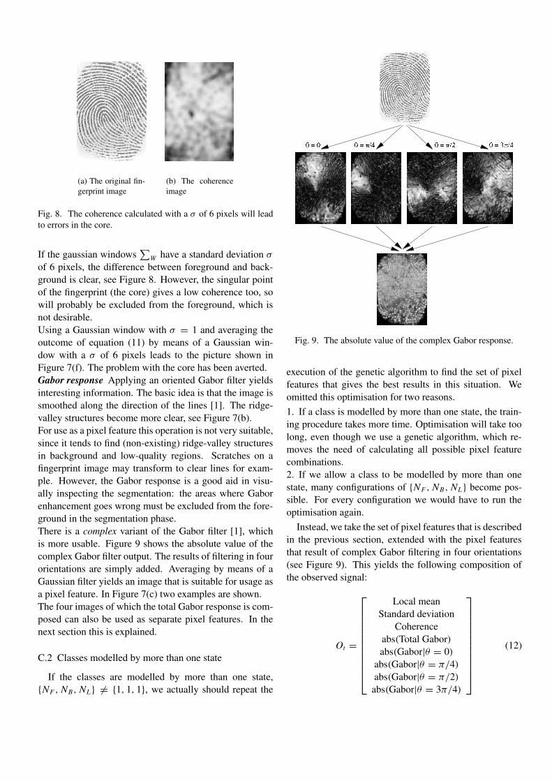
(a) The original fin-
gerprint image
(b) The coherence
image
Fig. 8. The coherence calculated with a σ of 6 pixels will lead
to errors in the core.
If the gaussian windows∑
W have a standard deviation σ
of 6 pixels, the difference between foreground and back-
ground is clear, see Figure 8. However, the singular point
of the fingerprint (the core) gives a low coherence too, so
will probably be excluded from the foreground, which is
not desirable.
Using a Gaussian window with σ = 1 and averaging the
outcome of equation (11) by means of a Gaussian win-
dow with a σ of 6 pixels leads to the picture shown in
Figure 7(f). The problem with the core has been averted.
Gabor response Applying an oriented Gabor filter yields
interesting information. The basic idea is that the image is
smoothed along the direction of the lines [1]. The ridge-
valley structures become more clear, see Figure 7(b).
For use as a pixel feature this operation is not very suitable,
since it tends to find (non-existing) ridge-valley structures
in background and low-quality regions. Scratches on a
fingerprint image may transform to clear lines for exam-
ple. However, the Gabor response is a good aid in visu-
ally inspecting the segmentation: the areas where Gabor
enhancement goes wrong must be excluded from the fore-
ground in the segmentation phase.
There is a complex variant of the Gabor filter [1], which
is more usable. Figure 9 shows the absolute value of the
complex Gabor filter output. The results of filtering in four
orientations are simply added. Averaging by means of a
Gaussian filter yields an image that is suitable for usage as
a pixel feature. In Figure 7(c) two examples are shown.
The four images of which the total Gabor response is com-
posed can also be used as separate pixel features. In the
next section this is explained.
C.2 Classes modelled by more than one state
If the classes are modelled by more than one state,
{NF , NB, NL} 6= {1, 1, 1}, we actually should repeat the
Fig. 9. The absolute value of the complex Gabor response.
execution of the genetic algorithm to find the set of pixel
features that gives the best results in this situation. We
omitted this optimisation for two reasons.
1. If a class is modelled by more than one state, the train-
ing procedure takes more time. Optimisation will take too
long, even though we use a genetic algorithm, which re-
moves the need of calculating all possible pixel feature
combinations.
2. If we allow a class to be modelled by more than one
state, many configurations of {NF , NB, NL} become pos-
sible. For every configuration we would have to run the
optimisation again.
Instead, we take the set of pixel features that is described
in the previous section, extended with the pixel features
that result of complex Gabor filtering in four orientations
(see Figure 9). This yields the following composition of
the observed signal:
Ot =
Local mean
Standard deviation
Coherence
abs(Total Gabor)
abs(Gabor|θ = 0)
abs(Gabor|θ = π/4)
abs(Gabor|θ = π/2)
abs(Gabor|θ = 3π/4)
(12)
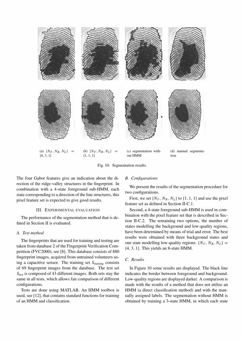
(a) {NF , NB , NL } =
{4, 3, 1}
(b) {NF , NB , NL } =
{1, 1, 1}
(c) segmentation with-
out HMM
(d) manual segmenta-
tion
Fig. 10. Segmentation results.
The four Gabor features give an indication about the di-
rection of the ridge-valley structures in the fingerprint. In
combination with a 4-state foreground sub-HMM, each
state corresponding to a direction of the line structures, this
pixel feature set is expected to give good results.
III. EXPERIMENTAL EVALUATION
The performance of the segmentation method that is de-
fined in Section II is evaluated.
A. Test method
The fingerprints that are used for training and testing are
taken from database 2 of the Fingerprint Verification Com-
petition (FVC2000), see [8]. This database consists of 880
fingerprint images, acquired from untrained volunteers us-
ing a capacitive sensor. The training set Straining consists
of 69 fingerprint images from the database. The test set
Stest is composed of 43 different images. Both sets stay the
same in all tests, which allows fair comparison of different
configurations.
Tests are done using MATLAB. An HMM toolbox is
used, see [12], that contains standard functions for training
of an HMM and classification.
B. Configurations
We present the results of the segmentation procedure for
two configurations.
First, we set {NF , NB, NL} to {1, 1, 1} and use the pixel
feature set as defined in Section II-C.1.
Second, a 4-state foreground sub-HMM is used in com-
bination with the pixel feature set that is described in Sec-
tion II-C.2. The remaining two options, the number of
states modelling the background and low-quality regions,
have been determined by means of trial and error. The best
results were obtained with three background states and
one state modelling low-quality regions: {NF , NB, NL} =
{4, 3, 1}. This yields an 8-state HMM.
C. Results
In Figure 10 some results are displayed. The black line
indicates the border between foreground and background.
Low-quality regions are displayed darker. A comparison is
made with the results of a method that does not utilise an
HMM (a direct classification method) and with the man-
ually assigned labels. The segmentation without HMM is
obtained by training a 3-state HMM, in which each state
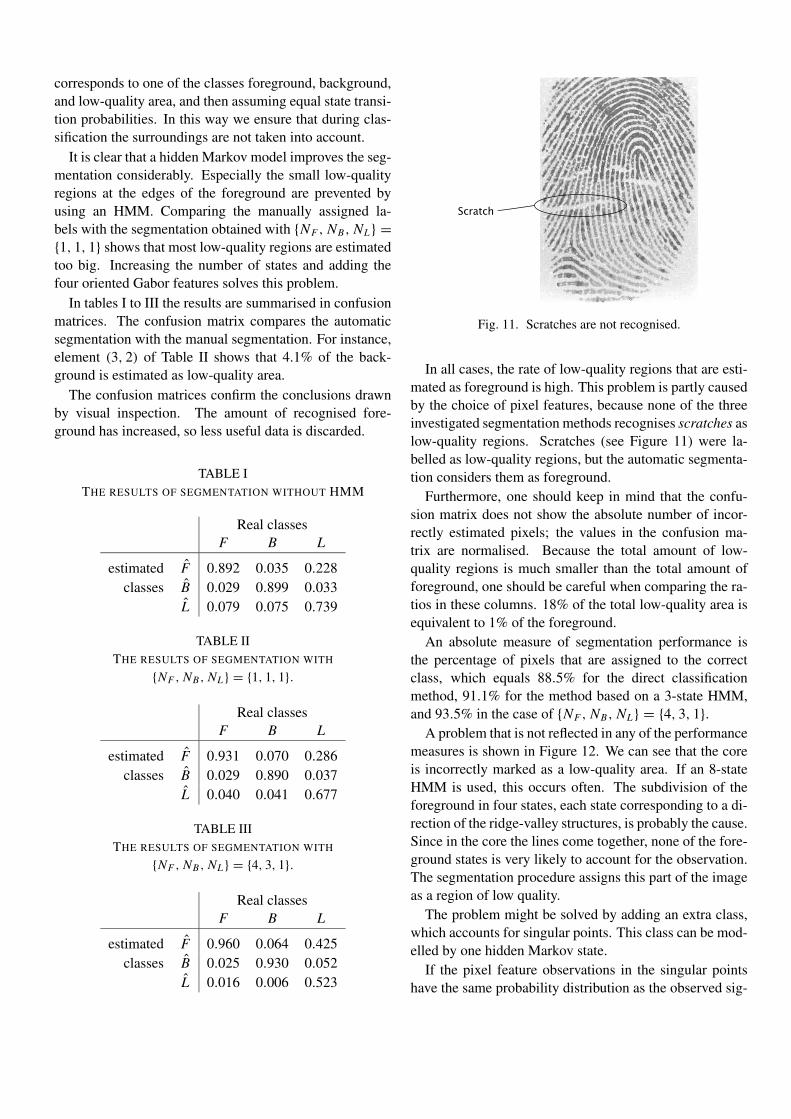
corresponds to one of the classes foreground, background,
and low-quality area, and then assuming equal state transi-
tion probabilities. In this way we ensure that during clas-
sification the surroundings are not taken into account.
It is clear that a hidden Markov model improves the seg-
mentation considerably. Especially the small low-quality
regions at the edges of the foreground are prevented by
using an HMM. Comparing the manually assigned la-
bels with the segmentation obtained with {NF , NB, NL} =
{1, 1, 1} shows that most low-quality regions are estimated
too big. Increasing the number of states and adding the
four oriented Gabor features solves this problem.
In tables I to III the results are summarised in confusion
matrices. The confusion matrix compares the automatic
segmentation with the manual segmentation. For instance,
element (3, 2) of Table II shows that 4.1% of the back-
ground is estimated as low-quality area.
The confusion matrices confirm the conclusions drawn
by visual inspection. The amount of recognised fore-
ground has increased, so less useful data is discarded.
TABLE I
THE RESULTS OF SEGMENTATION WITHOUT HMM
Real classes
F B L
estimated F 0.892 0.035 0.228
classes B 0.029 0.899 0.033
L 0.079 0.075 0.739
TABLE II
THE RESULTS OF SEGMENTATION WITH
{NF , NB , NL} = {1, 1, 1}.
Real classes
F B L
estimated F 0.931 0.070 0.286
classes B 0.029 0.890 0.037
L 0.040 0.041 0.677
TABLE III
THE RESULTS OF SEGMENTATION WITH
{NF , NB , NL} = {4, 3, 1}.
Real classes
F B L
estimated F 0.960 0.064 0.425
classes B 0.025 0.930 0.052
L 0.016 0.006 0.523
Scratch
Fig. 11. Scratches are not recognised.
In all cases, the rate of low-quality regions that are esti-
mated as foreground is high. This problem is partly caused
by the choice of pixel features, because none of the three
investigated segmentation methods recognises scratches as
low-quality regions. Scratches (see Figure 11) were la-
belled as low-quality regions, but the automatic segmenta-
tion considers them as foreground.
Furthermore, one should keep in mind that the confu-
sion matrix does not show the absolute number of incor-
rectly estimated pixels; the values in the confusion ma-
trix are normalised. Because the total amount of low-
quality regions is much smaller than the total amount of
foreground, one should be careful when comparing the ra-
tios in these columns. 18% of the total low-quality area is
equivalent to 1% of the foreground.
An absolute measure of segmentation performance is
the percentage of pixels that are assigned to the correct
class, which equals 88.5% for the direct classification
method, 91.1% for the method based on a 3-state HMM,
and 93.5% in the case of {NF , NB, NL} = {4, 3, 1}.
A problem that is not reflected in any of the performance
measures is shown in Figure 12. We can see that the core
is incorrectly marked as a low-quality area. If an 8-state
HMM is used, this occurs often. The subdivision of the
foreground in four states, each state corresponding to a di-
rection of the ridge-valley structures, is probably the cause.
Since in the core the lines come together, none of the fore-
ground states is very likely to account for the observation.
The segmentation procedure assigns this part of the image
as a region of low quality.
The problem might be solved by adding an extra class,
which accounts for singular points. This class can be mod-
elled by one hidden Markov state.
If the pixel feature observations in the singular points
have the same probability distribution as the observed sig-
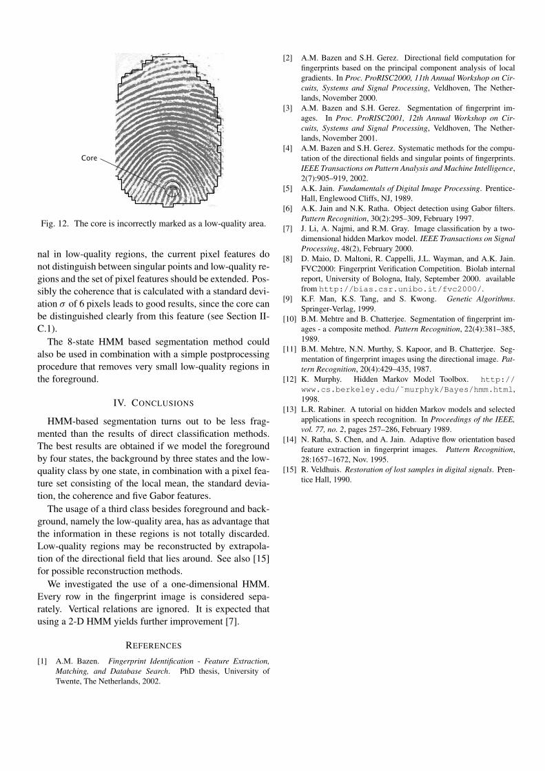
Core
Fig. 12. The core is incorrectly marked as a low-quality area.
nal in low-quality regions, the current pixel features do
not distinguish between singular points and low-quality re-
gions and the set of pixel features should be extended. Pos-
sibly the coherence that is calculated with a standard devi-
ation σ of 6 pixels leads to good results, since the core can
be distinguished clearly from this feature (see Section II-
C.1).
The 8-state HMM based segmentation method could
also be used in combination with a simple postprocessing
procedure that removes very small low-quality regions in
the foreground.
IV. CONCLUSIONS
HMM-based segmentation turns out to be less frag-
mented than the results of direct classification methods.
The best results are obtained if we model the foreground
by four states, the background by three states and the low-
quality class by one state, in combination with a pixel fea-
ture set consisting of the local mean, the standard devia-
tion, the coherence and five Gabor features.
The usage of a third class besides foreground and back-
ground, namely the low-quality area, has as advantage that
the information in these regions is not totally discarded.
Low-quality regions may be reconstructed by extrapola-
tion of the directional field that lies around. See also [15]
for possible reconstruction methods.
We investigated the use of a one-dimensional HMM.
Every row in the fingerprint image is considered sepa-
rately. Vertical relations are ignored. It is expected that
using a 2-D HMM yields further improvement [7].
REFERENCES
[1] A.M. Bazen. Fingerprint Identification - Feature Extraction,
Matching, and Database Search. PhD thesis, University of
Twente, The Netherlands, 2002.
[2] A.M. Bazen and S.H. Gerez. Directional field computation for
fingerprints based on the principal component analysis of local
gradients. In Proc. ProRISC2000, 11th Annual Workshop on Cir-
cuits, Systems and Signal Processing, Veldhoven, The Nether-
lands, November 2000.
[3] A.M. Bazen and S.H. Gerez. Segmentation of fingerprint im-
ages. In Proc. ProRISC2001, 12th Annual Workshop on Cir-
cuits, Systems and Signal Processing, Veldhoven, The Nether-
lands, November 2001.
[4] A.M. Bazen and S.H. Gerez. Systematic methods for the compu-
tation of the directional fields and singular points of fingerprints.
IEEE Transactions on Pattern Analysis and Machine Intelligence,
2(7):905–919, 2002.
[5] A.K. Jain. Fundamentals of Digital Image Processing. Prentice-
Hall, Englewood Cliffs, NJ, 1989.
[6] A.K. Jain and N.K. Ratha. Object detection using Gabor filters.
Pattern Recognition, 30(2):295–309, February 1997.
[7] J. Li, A. Najmi, and R.M. Gray. Image classification by a two-
dimensional hidden Markov model. IEEE Transactions on Signal
Processing, 48(2), February 2000.
[8] D. Maio, D. Maltoni, R. Cappelli, J.L. Wayman, and A.K. Jain.
FVC2000: Fingerprint Verification Competition. Biolab internal
report, University of Bologna, Italy, September 2000. available
from http://bias.csr.unibo.it/fvc2000/.
[9] K.F. Man, K.S. Tang, and S. Kwong. Genetic Algorithms.
Springer-Verlag, 1999.
[10] B.M. Mehtre and B. Chatterjee. Segmentation of fingerprint im-
ages - a composite method. Pattern Recognition, 22(4):381–385,
1989.
[11] B.M. Mehtre, N.N. Murthy, S. Kapoor, and B. Chatterjee. Seg-
mentation of fingerprint images using the directional image. Pat-
tern Recognition, 20(4):429–435, 1987.
[12] K. Murphy. Hidden Markov Model Toolbox. http://
www.cs.berkeley.edu/˜murphyk/Bayes/hmm.html,
1998.
[13] L.R. Rabiner. A tutorial on hidden Markov models and selected
applications in speech recognition. In Proceedings of the IEEE,
vol. 77, no. 2, pages 257–286, February 1989.
[14] N. Ratha, S. Chen, and A. Jain. Adaptive flow orientation based
feature extraction in fingerprint images. Pattern Recognition,
28:1657–1672, Nov. 1995.
[15] R. Veldhuis. Restoration of lost samples in digital signals. Pren-
tice Hall, 1990.
Bibliography
[1] L.E. Baum and G.R. Sell. Growth functions for transformations onmanifolds. Pac. J. Math., 27(2):211–227, 1968.
[2] A.M. Bazen. Fingerprint Identification - Feature Extraction, Matching,and Database Search. PhD thesis, University of Twente, The Nether-lands, 2002.
[3] A.M. Bazen and S.H. Gerez. Directional field computation for finger-prints based on the principal component analysis of local gradients. InProc. ProRISC2000, 11th Annual Workshop on Circuits, Systems andSignal Processing, Veldhoven, The Netherlands, November 2000.
[4] A.M. Bazen and S.H. Gerez. Segmentation of fingerprint images. InProc. ProRISC2001, 12th Annual Workshop on Circuits, Systems andSignal Processing, Veldhoven, The Netherlands, November 2001.
[5] A.M. Bazen and S.H. Gerez. Systematic methods for the computa-tion of the directional fields and singular points of fingerprints. IEEETransactions on Pattern Analysis and Machine Intelligence, 2(7):905–919, 2002.
[6] J. de Boer, A.M. Bazen, and S.H. Gerez. Indexing fingerprint databasesbased on multiple features. In Proc. ProRISC2001, 12th AnnualWorkshop on Circuits, Systems and Signal Processing, Veldhoven, TheNetherlands, November 2001.
[7] Olivier Cappe. H2M: A set of MATLAB/OCTAVE functions for theEM estimation of mixtures and hidden Markov models, August 24 2001.
[8] Zoubin Ghahramani and Michael I. Jordan. Supervised learning fromincomplete data via an EM approach. In Jack D. Cowan, GeraldTesauro, and Joshua Alspector, editors, Advances in Neural Informa-tion Processing Systems, volume 6, pages 120–127. Morgan KaufmannPublishers, Inc., 1994.
[9] A.K. Jain. Fundamentals of Digital Image Processing. Prentice-Hall,Englewood Cliffs, NJ, 1989.
108 Bibliography
[10] A.K. Jain and N.K. Ratha. Object detection using Gabor filters. Pat-tern Recognition, 30(2):295–309, February 1997.
[11] J. Li, A. Najmi, and R.M. Gray. Image classification by a two-dimensional hidden Markov model. IEEE Transactions on Signal Pro-cessing, 48(2), February 2000.
[12] D. Maio, D. Maltoni, R. Cappelli, J.L. Wayman, and A.K. Jain.FVC2000: Fingerprint Verification Competition. Biolab internal re-port, University of Bologna, Italy, September 2000. available fromhttp://bias.csr.unibo.it/fvc2000/.
[13] K.F. Man, K.S. Tang, and S. Kwong. Genetic Algorithms. Springer-Verlag, 1999.
[14] B.M. Mehtre and B. Chatterjee. Segmentation of fingerprint images -a composite method. Pattern Recognition, 22(4):381–385, 1989.
[15] B.M. Mehtre, N.N. Murthy, S. Kapoor, and B. Chatterjee. Segmenta-tion of fingerprint images using the directional image. Pattern Recog-nition, 20(4):429–435, 1987.
[16] T.K. Moon and W.C. Stirling. Mathematical Methods and Algorithmsfor Signal Processing. Prentice Hall, Upper Saddle River, NJ, 2000.
[17] S. Muller, S. Eickeler, C. Neukirchen, and B. Winterstein. Segmentationand classification of hand-drawn pictograms in cluttered scenes - anintegrated approach.
[18] K. Murphy. Hidden Markov Model Toolbox. http://www.cs.berkeley.edu/~murphyk/Bayes/hmm.html, 1998.
[19] A.V. Nefian and M.H. Hayes. Face recognition using an embeddedHMM. In Proceedings of the IEEE Conference on Audio and Video-based Biometric Person Authentication, pages 19–24, March 1999.
[20] L.R. Rabiner. A tutorial on hidden Markov models and selected appli-cations in speech recognition. In Proceedings of the IEEE, vol. 77, no.2, pages 257–286, February 1989.
[21] L.R. Rabiner and B.H. Juang. Fundamentals of speech recognition.Prentice Hall, 1993.
[22] N. Ratha, S. Chen, and A. Jain. Adaptive flow orientation based featureextraction in fingerprint images. Pattern Recognition, 28:1657–1672,Nov. 1995.
[23] R. Veldhuis. Restoration of lost samples in digital signals. PrenticeHall, 1990.

Bibliography 109
[24] R. Veldhuis and M. Breeuwer. An introduction to source coding. Pren-tice Hall, 1993.