finite deformation plasticity for composite structures: computational models and adaptive strategies

ELSEVIER

Computer methods in applied

mechanics and engineerlng

Comput. Methods Appl. Mech. Engrg. 172 (1999) 145-174

Finite deformation plasticity for composite structures: Computational models and adaptive strategies

Jacob Fish*, Kamlun Shek Departments of Civil, Mechanical and Aerospace Engineering, Rensselaer Polytechnic Institute, Troy, NY 12180, USA

Received 1 June 1998

Abstract

We develop computational models and adaptive modeling strategies for obtaining an approximate solution to a boundary value problem describing the finite deformation plasticity of heterogeneous structures. A nearly optimal mathematical model consists of an averaging scheme based on approximating eigenstrains and elastic concentration factors in each micro phase by a constant in the portion of the macro-domain where modeling errors are small, whereas elsewhere, a more detailed mathematical model based on a piecewise constant approximation of eigenstrains and elastic concentration factors is utilized. The methodology is developed within the framework of ‘statistically homogeneous’ composite material and local periodicity assumptions. 0 1999 Elsevier Science S.A. All rights reserved.

1. Introduction

In this manuscript, we develop a theory and methodology for obtaining an approximate solution to a boundary value problem describing the finite deformation plasticity of heterogeneous structures. The theory is developed within the framework of ‘statistically homogeneous’ composite material and local periodicity assumptions. For readers interested in theoretical and computational issues dealing with various aspects of nonperiodic heterogeneous media we refer to [7,9,28,37].

The challenge of solving structural problems with accurate resolution of microstructural fields undergoing inelastic deformation is enormous. This subject has been an active area of research in the computational mechanics community for more than two decades. Numerous studies have dealt with the utilization of the finite element method [ 12,13,18,2 1,22,24,30,34], the boundary element method [ 111, the Voronoi cell method [ 101, the spectral method [l], the transformation field analysis [5], and the Fourier series expansion technique [26] for solving PDEs arising from the homogenization of nonlinear composites. The primary goals of these studies were twofold: (i) develop macroscopic constitutive equations that would enable solution of an auxiliary problem with nonlinear homogenized (smooth) coefficients; and (ii) establish bounds for overall nonlinear properties [2,29,32-351.

Attempts at solving large-scale nonlinear structural systems with accurate resolution of microstructural fields are very rare [10,12,26] and successes were reported for small problems and/or special cases. This is because for linear problems a unit cell or a representative volume problem has to be solved only once, whereas for nonlinear history dependent systems, it has to be solved at every increment and for each macroscopic (Gauss) point. Furthermore, history data has to be updated at a number of integration points equal to the product of the number of Gauss points in the macro and micro (unit cell) domains.

To illustrate the computational complexity involved we consider an elasto-plastic analysis of the composite

* Cotresponding author.

0045.7825 /99/$ - see front matter 0 1999 Elsevier Science S.A. All rights reserved. PII: SOO45-7825(98)00228-X

146 J. Fish, K. Shek I Comput. Methods Appl. Mech. Engrg. 172 (1999) 145-174

Fig. 1. Finite element mesh for the nozzle flap problem. Fig. 2. Finite element mesh for the fibrous unit cell

flap problem [8] with fibrous microstructure as shown in Figs. 1 and 2. The structural problem is discretized with 788 tetrahedral elements (993 degrees of freedom), whereas fibrous microstructure is discretized with 98 elements in the fiber domain and 253 elements in the matrix domain, totaling 330 degrees of freedom. The CPU time on SPARC lo/51 workstation for this problem was over 7 hours, as opposed to 10 seconds if von Mises metal plasticity was used instead, which means that 99.9% of CPU time is spent on stress updates.

With the exception of [6,12,19] most of the research activities focused on small deformation inelastic response of microconstituents and their interfaces. This is partially justified due to high stiffness and relatively low ductility of fibrous composite materials. However, when hardening is low and the stress measures are comparable to the inelastic tangent modulus, or in the case of thin structures undergoing large rotations, large deformation formulation is required.

One of the objectives of the present manuscript is to extend the recent formulation of the mathematical homogenization theory with eigenstrains developed by the authors in [8] to account for finite deformation and thermal effects. In addition, adaptive strategy is devised to ensure reliability and efficiency of computations. In Section 2 we derive a closed form expression relating arbitrary transformation fields to mechanical fields in the phases. In Sections 3 and 4 we employ an additive decomposition of the rate of deformation into elastic rate of deformation, governed by hypoelasticity and inelastic rate of deformation. Section 3 focuses on the 2-point approximation scheme (for two phase materials), where each point represents an average response within a phase. The local response within each phase is then recovered by means of post-processing. In Section 4 we describe the n-point scheme model, where n denotes the number of elements in the microstructure. Section 5 is devoted to modeling error estimation and adaptive strategy. We develop an adaptive 2 /n-point model, where the 2-point scheme is used in regions where modeling errors are small, whereas elsewhere the n-point scheme is employed. Numerical experiments conducted in Section 6 investigate the 2-point, the n-point, and the adaptive 2/n-point schemes in the context of finite deformation plasticity.

2. Mathematical homogenization with eigenstrains for small deformations

In this section we generalize the classical mathematical homogenization theory [3,4] for heterogeneous media to account for eigenstrains. We regard all inelastic strains, phase transformation and temperature effects as eigenstrains in an otherwise elastic body. We will derive closed-form expressions relating arbitrary eigenstrains to mechanical fields in a multi-phase composite medium. In this section attention is restricted to small deformations.

The microstructure of a composite material is assumed to be locally periodic (Y-periodic) with a period represented by a unit cell domain or a Representative Volume Element (RVE), denoted by 0, as shown in Fig. 3. Let x be a macroscopic coordinate vector in macro domain fi and y =x /IJ be a microscopic position vector in 0. For any Y-periodic function J we have f(x, y) =f(x, y + ki) in which vector y^ is the basic period of the microstructure and k is a 3 by 3 diagonal matrix with integer components. Adopting the classical nomenclature, any Y-periodic function f can be represented as

.I. Fish, K. Shek I Comput. Methods A&. Mech. Engrg. 172 (1999) 145 I74 147

Fig. 3. Macroscopic and microscopic structures.

f”(x) =m Y(X)> (1)

where superscript l denotes a Y-periodic function fi The indirect macroscopic spatial derivatives off % can be calculated by the chain rule as

ffY$> -.lyx~ Y) =f& Y> + $ fy,(x, Y) (2)

&(x9 Y) =f& Y> + !&(x9 Y) = !cJJX> Y) (3)

where the comma followed by a subscript variable xi or yi denotes a partial derivative with respect to the subscript variable (i.e.fX = c?$/&x; andf, = af/ay,). A semi-colon followed by a subscript variable xi denotes a partial derivative with respect to the remaining x components (2), but a full derivative with respect to yi, and vice versa when a semicolon is followed by subscript variable yi (3). Summation convention for repeated right-hand side subscripts is employed, except for subscripts x and y.

We assume that micro-constituents possess homogeneous properties and satisfy equilibrium, constitutive, kinematics and compatibility equations as well as jump conditions at the interface between the micro-phases. The corresponding boundary value problem is governed by the following equations:

ai:, + bi = 0 in 0 (4)

gli = L&L -pfI,) in0 (5) 5 i

&ij = ‘(i;x,) in 0 (6)

c i wij = ‘[i:x,l in .fJ (7)

ui=u I 1 on r, (8)

+, =t, on c (9)

where (T:, C: and w: are components of stress, strain and rotation tensors; Lijk, and ,ui are components of elastic stiffness and eigenstrain tensors, respectively; bi is a body force assumed to be independent of y; Z.L~ denotes the components of the displacement vector; the subscript pairs with regular and square parenthesizes denote the symmetric and anti-symmetric gradients defined as

/& ) = - (10) I ; “f.., + u;J, &,, +4+ -&>

0 denotes the macroscopic domain of interest with boundary P, K and 4 are boundary portions where displacements U, and tractions ii are prescribed, respectively, such that c fl c = 0 and r = c U 4; n, denotes the normal vector on r We assume that the interface between the phases is perfectly bonded, i.e. [ahr;l] = 0 and [u:] = 0 at the interface, Tnt, where Gi is the normal vector to q,,, and [*I is a jump operator.

In the following, displacements U;(X) = U&C, y) and eigenstrains ,L&) = pij(x, y) are approximated in terms of double scale asymptotic expansions on 0 X 0:

148 .I. Fish, K. Shek I Comput. Methods Appl. Mech. Engrg. 172 (1999) 145-174

Strain and rotation expansions on 0 X 0 can be obtained by substituting (11) into (6) and (7) with consideration of the indirect differentiation rule (2)

Eij(X, y) = $ &,- ’ (x, y) + $(x, y) + &(x, y) + . . . (13)

w;,(x3 Y) = j cq(x, y) + wo,(x, y) + &JfJ(x, y) + . * * (14)

where strain and rotation components for the various orders of 5 are given as

&,; ’ = &yij(uo> ) &:, = Exi,(zL) + &yij(u”+‘), s = 0, 1,. . . (15)

qy = wyij(uo) 3 w; = oJxij(U”) + wy,-(us+‘), s = 0, 1,. . . (16)

and

E*rj(““) = ‘;i,x,) ) Eylj(us) = ‘;i,y,) (17)

wxij(““> = ‘si,x,] 3 wyi~(““) = ‘;i,y,] (18)

Stresses and strains for different orders of 5 are related by the constitutive equation (5)

CT;’ = L*jklEL’ 3 CT; = Li,J&;, - p;,> ) s = 0, 1, . . . (19)

The resulting asymptotic expansion of stress is given as

q,k Y) = $ cq(x, y) + +, y) + g/(x, y) + . . . (20)

Inserting the stress expansion (20) into equilibrium equation (4) and making the use of (2) yields the following equilibrium equations for various orders:

O( 5-“): a,;, = 0 (21)

O( 5-Q: u;,;, + a;,,, = 0 (22)

0( 5”): CT;,+ + u,;,~, + b, = 0 (23)

O( 5”): c&, + ur;r:, = 0 ) s = 1,2, . . . (24)

Consider the 0( l-*) equilibrium equation (21) first. Pre-multiplying it by UP and integrating over a unit cell domain 0 yields

and subsequently integrating by parts gives

(25)

(26)

where r, denotes the boundary of 0. The boundary integral term in (26) vanishes due to Y-periodicity of boundary conditions on r,. Furthermore, since the elastic stiffness Lijkr is positive definite, we have

0 u(,,y,) = 0 =3 up = L&x, (27)

and

a,‘(X,y)=F,I’(X,y)=W,‘(X,y)=O (28)

We proceed to the O([-‘) equilibrium equation (22) next. From Eqs. (15) and (19) follows

J. Fish, K. Shek / Comput. Methods Appl. Mech. Engrg. 172 (1999) 145-174 149

&jklkkl(~o) + &ykl(~‘) - &)l,, = 0 on @ (29)

To solve for (29) up to a constant we introduce the following separation of variables

4(x7 Y> = Y.kl(Y){qkl@“) + d3d (30)

where Hikl is a Y-periodic function, d: is a macroscopic portion of the solution resulting from eigenstrains, i.e. if ,&(x, y) = 0 then d:(x) = 0. It should be noted that both Hikl and dc[ are symmetric with respect to indices k and 1. Based on (30) 0( 5 -‘) equilibrium equation takes the following form:

{Lijkl((zklmn + Gklmn >G&~) + G+,z,d~,(~) - ru;&, = 0 on @ (31)

where

Z klmn = ; @,,& + s,,s,,> > Gklmn(y) = H(k,y,)mn(y) (32)

and S,, is the Kronecker delta. Since Eq. (3 1) should be valid for arbitrary combination of macroscopic strain field E,,,(u’) and eigenstrain field &, we first consider & = 0, E,,,(u’) # 0 and then E,,,(u’) = 0, & # 0 which yields the following two governing equations on 0:

{Lijkl(zklmn + H(k,y,)mn)),y, = ’ (33)

{Lijkl(H(k,y,hnd~n - pil)},y, = ’ (34)

Eq. (33) together with Y-periodic boundary conditions comprise a standard linear boundary value problem on 0. For complex microstructures the finite element method is often employed for discretization of Hikl(y), which yields a set of linear algebraic system with six right-hand side vectors [7]. In absence of eigenstrains, the asymptotic fields can be written in terms of the macroscopic strain zij = E,~~(u’) and the macroscopic rotation oij = wx,(uO>:

qj =Zij + GijklE,, + 0( 5) ,

where

q, =Tqj + ei,klzkl + O( 5) (35)

n Gijkl(Y) = H[i,y,]kl(Y) (36)

The terms G,,, and Gijkl are known as polarization functions. It can be shown that the integrals of the polarization functions on 0 vanish due to periodicity conditions.

The elastic homogenized stiffness Lijkl follows from 0( 3’) equilibrium equation [7]:

AmnijLmnsrAstk, d@

where

A klmn = I klmn + Gklmn (38)

A klmn is often referred to as an elastic strain concentration function and 101 is the volume of a unit cell. After solving (33) for Hi,,, we proceed to (34) for finding dcl subjected to Y-periodic boundary conditions.

Pre-multiplying (34) by Hi,, and then integrating the resulting equation by parts with consideration of Y-periodic boundary conditions yields

I GijstLijkl(Gklmnd~n(~X) - /‘!I) d@ = 0 (39) e

Rewriting (39) in terms of strain concentration function Aijkr and manipulating it with (37) yields


where

(41)

The superscript - 1 denotes the reciprocal tensor. The 0( 5”) approximation to the asymptotic strain (13) and rotation fields (14) reduces to

Eij =‘,I + Gijkl(zkl + ‘cl + O(l) (42)

w;, =w, + c3;rjkl(zkl + q/) + O( [) (43)

Let $-{Jl’“‘(y)}~ be a set of C-’ continuous functions, then the separation of variables for the O(l”) eigenstrains is assumed to have the following decomposition:

&(X? Y> = il $(“)(Yh&%) (44)

The resulting asymptotic expansion of the strain and rotation fields (13), (14) can be expressed as follows:

where D$;(y) and fiz$y) are the eigenstrain influence functions, which can be expressed in terms of polarization functions Gijk,(y) and Gjjkl(y) as follows:

)-I s, GrspqLrsk, $@‘I d @

In particular, if (I; is a set of piecewise constant functions defined as

$wY,) = 1 if yP E O(‘) 0 otherwise

(47)

(48)

(49)

and O(‘) is the subdomain 77 within a unit cell, c (‘) the subdomain volume fraction given by c(” = 1 @(‘)I / 1 O( and satisfying IX:=, c (” = 1 then (45) and (46) reduce to ,

and

(53)

We will refer to the piecewise constant model defined by (50) as the n-point scheme model. Eq. (50a) has been

J. Fish, K. Shek I Comput. Methods Appl. Mech. Engrg. 172 (1999) 145-174 151

originally derived by Dvorak [5] on the basis of transformation field analysis. Finally, we integrate the 0( 5”) equilibrium equation (23) over 0. The Jo u,:,~, d@ term vanishes due to periodicity and we obtain:

(&/Ogid@),X,+bi=O on0 (54)

Substituting the constitutive relation (19) and the asymptotic expansion of strain tensor (42) into the above equation yields the macroscopic equilibrium equation

Finally, if we define the macroscopic stress a, as

- qj+, /rp,dO

I

then the equilibrium equations (54) and (55) can be further simplified as follows:

i& + bi = 0 , {‘ijkt(‘kt -Zkl)I,x, + bi = 0

where L, is the overall eigenstrain given by

(56)

(57)

Replacing Gmnpq by Amnpy - Lnpq and manipulating (58) with (37) and (40), the overall eigenstrain field can be expressed as

L, = & o BklijPil d@ 3 I B,,t = Lij,,(Y)A,,,,(Y)‘,-b,t (59)

Eq. (59) represents the well-known Levin’s formula [23] relating the local and overall eigenstrains, and Bi,kl is often referred to as the elastic stress concentration function.

REMARK 1. As a special case we consider a composite medium consisting of two phases, matrix and reinforcement, with respective volume fractions cCm) and ccf’ such that cCm) + cCf) = 1. Superscripts m and f represent matrix and reinforcement phases, respectively. OCm) and @’ denote the matrix and reinforcement domains such that 0 = 0’“’ U @‘. We assume that eigenstrains and elastic strain concentration factors are constant within each phase. This yields the simplest variant of (50) where IZ = 2. The corresponding approximation scheme is termed as the 2-point model. The overall elastic properties are given by [5]

and the overall stress reduces to

5, = pog(,y’ + ,(f),(f) ‘J ‘I ‘I

3. 2-Point scheme for finite deformation plasticity

(60)

(61)

For finite deformation analysis the left superscript denotes the configuration: r+AtO is the current configuration at time t + At, whereas ‘0 is the configuration at time t. For simplicity, we will often omit the left superscript for the current configuration, i.e. 0 = t+AiltCi. To extend the small deformation formulation to account for finite deformation effects the following assumptions are made:

Al:, Phase stress objectivity

152 J. Fish, K. Shek I Comput. Methods Appl. Mech. Engrg. 172 (1999) 145-l 74

We will assume that the principle of objectivity is satisfied for each phase. Then the Cauchy stress rate for phase r is given as

,(I) = &I) + p ‘I ‘I lJ

where ci, i(r) = /Qyg; - &;‘A; (62)

where the superposed dot represents the material time derivative. The rate of deformation and spin tensor .p

components, denoted as cij . p

and wij , respectively, are defined as

q(X) = u ;;y,, and ti$r)(x) = u fiE,, (63)

where u,‘.:’ is the phase velocity gradient. The asymptotic expansion of the phase velocity is given as I

ly)(x) = u;“(x, y) = 7y(x, y) + &y’(x, y) + . . . (64)

+) is the objective rate of the Cauchy stress in phase r, which represents the material response due to z&ormation, whereas AI;” = %~;‘{%~}-’ represents the rate of rotation.

REMARK 2. The optimal choice of rotation 8::) depends on the microstructure. For fibrous composites it is natural to assume that nZ:J), represents the fiber rotation from the configuration aligned along the unit vector ‘m, to the current configuration aligned along the vector m,. Thus

Following Lee [20] it can be shown that $’ is related to the spin and rate of deformation tensors by

Jip) = ,w + ,!r) . (r) ?I ?I rk mkmj - &jk mkmi (66)

The choice of rotations in textile and particle composites is less obvious. We refer to Hughes [16] for the discussion on various choices.

A2: Additive decomposition of hypoelastic and inelastic rate of deformation The theoretical and practical reasons favoring additive decomposition over multiplicative decomposition for

fibrous composites were discussed in [27]. In the present work we adopt the additive decomposition of rate of deformation into elastic e.GiJ’ and inelastic rate of deformation hi;), which gives

,(I) = $‘I + ,(:I ?I e ?I ‘J (67)

Furthermore, we will assume the hypoelastic constitutive equation relating the objective Cauchy stress rate with rate of elastic deformation:

8;;’ zz L$,@ - &‘) (68)

A3: Midpoint integration scheme for micro- and macro-coordinates In a typical time step t + At, the configuration of the macro- and micro-structure may be expressed as a sum

of the configuration at the previous step t and the displacement increment:

‘+‘;Ci = ;ci + Au; (69)

r+Aryi = ryi + At& (70)

The macroscopic displacement increment Au: is found from the incremental solution of the macro-problem, whereas displacement increment in the RVE is given by

A&(x, y) = {A,(x) + AOij(x)}yj + Auf (x, y) (71)

The first term in (71) represents the contribution of macroscopic solution, whereas the second term Au~(x, y) accounts for oscillatory Y-periodic field. Fig. 4 schematically illustrates the decomposition of the deformation field in the RVE.

Strain and rotation increments are integrated using the midpoint rule to obtain a second-order accuracy:

.I. Fish, K. Shek I Comput. Methods Appl. Mech. Engrg. 172 (1999) 145-174 153

(a) Undcfd d~atica @‘Shticm k) “XP al

Fig. 4. Decomposition of deformation in the microstructure.

&Gij = L f3AUp 1 8AUp 8AUJ”

2 fg r+At/2 AOij = - 2 #+At/2 -

x, dr+Ar’2 ‘i

(72)

where the midpoint coordinates are defined as

1+Ar12 xi =; (;ci + r+AtX,) , r+A3 =; (ty, + ‘+Aryi) (73)

Similarly, the periodic portion of the solution increment Auf is obtained by integrating (30) using the midpoint rule:

Azq! = I&,,( “A”2y)(A,,(x) + Ad:,(x)) (74)

where the increment of inelastic strain is defined in Section 4.

A4: Additive decomposition of material and rotational response There are several formulations aimed at extending the small deformation formulation to account for large

deformation effects. One of the most popular approaches is known as the co-rotational method where all the fields of interest are transformed into the rotated %-system [16]. In the %-system, the form of constitutive equations is analogous to small deformation theory. A simpler approach, proposed by Hallquist [14] and improved by Hughes and Winget [17] to preserve incremental objectivity, is based on the additive incremental decomposition of material and rotational response. The latter procedure is adopted in the present manuscript.

For two-phase materials, the integration scheme [17] decomposes stresses and back stresses as follows:

(75)

(76)

where CX~J’ is the back stress. The midpoint rule is utilized to compute the phase rotations [17]

(77)

REMARK 3. For homogeneous materials the integration scheme [17] uncouples the material and rotational responses. In the present formulation phase rotations in each phase, %:I, depend on phase eigenstrains, which are unknown prior to stress integration, and thus material and rotational responses are fully coupled and have to be updated simultaneously.

A5: Constant phase volume fractions For the 2-point scheme derived in Section 3 we will assume that phase volume fractions remain constant

throughout the analysis. This is apparently true in the case of elastic fibers undergoing small strains and incompressible matrix material. In addition, we assume that the elastic properties of the phases are independent of temperature. Based on the first-order approximation methods, such as the Mori-Tanaka method [25] and Self Consistent method [ 151, the strain concentration factors and eigenstrain influence functions can be assumed to be constants throughout the entire analysis. These assumptions will allow us to carry out the entire analysis without updating the configuration of the unit cells. For the n-point scheme model, described in Section 4, these restrictions will be removed.

154 J. Fish, K. Shek I Comput. Methods Appl. Mech. Engrg. I72 (1999) 145 174

3.1. Implicit integration of constitutive equation

For the elastically deforming reinforcement the only source of eigenstrain rate is due to temperature effects, i.e. j.iijf’ = &lif’ where @lj’) is the thermal rate of deformation in reinforcement domain. The eigenstrain rate in the matrix phase is comprised of both the thermal, $r’, and the plastic, p&ij ‘@“), rate of deformation effects, such that ki,?’ = sEI,m’ + ,,$f,?). The phase thermal rate of deformation can be expressed as

@i.ij” = @ii (78)

where 13 denotes the temperature and $” are components of the phase thermal expansion tensor. Combining the rate form of (50), (68), (69), (75), Assumptions 3 and 4 it can be shown that the following

relations for the phase stresses hold:

f t+Afa!;) = ‘&-I;‘) + RI?:, A& - c Q$: A&’ , r = m, f (79) \ =m

where A,&’ is the overall phase eigenstrain increment and

Consider the yield function of the following form:

@ya;y - cq’, Y’“‘) = ; (a;,?) - cdJn))Pi&~) - “E)) - f {Y’“‘}2 (81)

where Y@) is the yield stress of the matrix phase in a uniaxial test, which evolves according to the hardening laws assumed; al,?) corresponds to the center of the yield surface in the deviatoric stress space, or simply the back stress. Evolution of the back stress is assumed to follow the kinematic hardening rule. For von Mises plasticity, P,,,, is a projection which transforms an arbitrary second-order tensor to the deviatoric space:

'ijkl = 'ij!it - f s;jskl (82)

For simplicity we assume that the plastic rate of deformation in the matrix phase follows the associative flow rule:

We adopt a modified version of the hardening evolution law [16] in the context of isotropic, homogeneous, elasto-plastic matrix phase. A scalar material dependent parameter p (0 S /3 s 1) is used as a measure of the proportion of isotropic and kinematic hardening and A’“’ is a plastic parameter to be determined by the consistency condition (81). Accordingly, the evolution of the yield stress Y (m) and the back stress o:J”’ can be expressed as follows:

Y ‘(ml = ?g y(m’~(m’

o(m) _ 21 - PV ‘yi, - 3

P,,,(c$ - cx~))h’(m)

(84)

where p = 0 corresponds to a pure isotropic hardening; /? = 1 is the widely used Ziegler-Prager kinematic hardening rule [36] for metals; h is a hardening parameter defined as the ratio between effective stress rate and the effective plastic strain rate.

Integration of (83), (84) and (85) is carried out using the backward Euler scheme:

J. Fish, K. Shek I Comput. Methods Appl. Mech. Engrg. 172 (1999) 145-174

r+At (m) _ f (m) p &ij - p&ij +

t+Ar@,y) Ah’“’

155

(86)

f+Afy(m) = fy(m, ; 2y r+Aym) AA’“’ (87)

‘ijkl( r+Ar (m)

(+kl _ f+Ara;y)) Ah(*)

where Ah(“) = f+Arh(*) _ fh(*) - and ‘&il?’ is the rotated back stress defined in (76). The phase rotation increment follows from (50), (78) and (;13):

In the following we omit the left superscript for the current step t + At. Using the backward Euler scheme for the rate form of ai;) . m (79) and (86) yields the following relation for the Cauchy stress in the matrix domain:

(p = Cm) !I tr"ij

- Q;S”,‘;‘“c’ Ah’“’ (90)

where &,y) is a trial Cauchy stress in the matrix phase defined as

f

tr”i, (m) = ‘$J”’ + Rj,;; Ak, - 2 Q!,;;‘s;’ A8 (91) s = m

The process is termed elastic if

(pjjm) - a$?))Pijkl(trcTp - (Ykl (m9 - 3 W”‘12 1 A*(m)=0 <cl (92)

Otherwise the process is plastic, which is the focus of our subsequent derivation. Subtracting (88) from (90) we arrive at the following result:

(TV ‘I - a;,?) = (I;,,, + Ah’“’ ~,kr)-‘(tra~’ - ‘&g’)

where

(93)

@,jk, = QiJ:“‘P,v,k, f 3 (1 - PjhPijkl (94)

The value of AA’“’ is obtained by satisfying the consistency condition which assures that the stress state in the plastic process lies on the yield surface at the end of the current load step. To this end, Eqs. (87) and (93) are substituted into the consistency condition (81), Gem)($) - al,“), Y’“‘) = 0, which produces a nonlinear equation for Ah’“‘. A standard Newton’s method is applied to solve for AA’“‘:

(95)

where k is the iteration count. It can be shown that the derivative a@‘“‘/ aAh’“’ required in (95) has the following form:

a cPm) ___ = qq?&Tp - $‘) - 4ph{Y’m’}2

dAA’“’ 9 - 6fih AA’“’ (96)

The expression for C$ is derived in Appendix A. The converged value of Ah (m) is then used to compute the phase stresses. The overall stress is computed from (61).

3.2. Consistent linearization

While integration of the constitutive equations affects the accuracy of the solution, the formation of a tangent stiffness matrix consistent with the integration procedure is essential to maintain the quadratic rate of

Subtracting

where

(98)

(99)

(100)

(101)

156 J. Fish, K. Shrk I Cornput. Methods Appl. Mech. Engrg. 172 (1999) 145-174

convergence if one is to adopt the Newton method for the solution of nonlinear system of equations on the macro level [3 11.

The starting point is the incremental form of the constitutive equations (79):

u;;’ = *,;;) + Rllk, cr) A-& - Qi;;‘X/i;“’ AA’“’ - ,\$ Q$: t;’ A0

Taking material time derivative of (88), (89) and (97) yields

(97)

I ;(m) , i(m) a( $T”’ - ;;):“‘) g,, - a! ‘, =

aA&J;’ A&C) (102)

Combining (99), (101 ), ( 102), (212), (213) with the consistent linearizations of A$, and A4, (given in Appendix B) yields

. (ml ui,, - ‘yii .(‘n) = (ztjk, + Ah’“’ Wj;;)-I( J,,,r,v;,x, + $,,d + &?) (103)

where

vsk,\, = Learn - JJ2” Wrmn,.sr + &,nuJ$uvv).J + &J%mw (104)

@Sk, = f: KJ$& - ,U:;J~::; - Q:i’i)l:‘>s:.;’ (105) .S=,E

,s,, = - w~v;(u;y’ - a;.;‘) (106)

and W$,, JJ~~,, and ,lJEL,, are defined in (217), (212) and (213), respectively. It remains to eliminate i’“’ from ( 103), by utilizing the linearized form of the consistency condition (8 1) and Eq. (87) which gives

)y( (Jy - &f,“‘) - 4ph{Y’“‘}*/P’ o

9 - 6ph AA’“’ =

Substituting (103) into (107) results in

A ‘w) = f Z’( vSkt,stv~,x, + @SklS)

where

(107)

(108)

p) = (9 - 6ph AA’“‘)K;;“‘(Z,,, + AA’“’ W;,;;)-’ kl 4~{Y’“‘}’ - (9 - 6/3/z AA(m))Kjnmn)(Zmns, + Ah’“’ Wzs,)-’ Js,

and thus (103) can be simplified as

(109)

.I. Fish, K. Shek I Comput. Methods Appl. Mech. Engrg. 172 (1999) 145- 174 157

(p) ‘I - c$,~ = “Sijk,z&, + ,&,d (110)

where

vSljk[ = (‘ijmn + A”“’ Kjmn)-‘(v’mnkl+ ,‘mn’K’ $‘pqkl) (111)

eSi/ = <I,,, + A’ W) &J’(gSmn + ,L,q l&J (112)

Finally, by substituting (108), (llO), (212) and (228) into (loo), we get a closed form expression relating the phase Cauchy stress rate ti-1’ with the macroscopic velocity gradient v:,,, and the temperature rate 4

&’ = D!‘;, v;,,, + d;i”fzj V (113)

(114)

+ Lr~I;;Y&m - Q;;::,W:;r;’ ,gSpq + AA’“’ P,j,npy &J (115)

The overall consistent instantaneous stiffness Dljk, is obtained from the rate form of (61) and Assumption A5: 1 uij=D.. v r,kl ix, + d,e (116)

where

D.. = ccm)D!m) + c(f’D(f’ r,kl rJkl r,kl )

d. = c(m,d(m, + c’,“d!” IJ ‘I ‘I (117)

The overall consistent tangent operator is derived from the consistent linearization of the weak form of the macroscopic equilibrium equation (57). Consider the internal force vector expressed in terms of the quantities defined in the deformed configuration

where Ni, is a set of shape functions in the macroscale. Prior to linearization, the internal force vector is defined in the reference configuration ‘0 as

where J, is the Jacobian between the macro-configurations at times t and t + At; Fjm is the macroscopic deformation gradient defined as

F,m = xj rx = r+Afxj, ,x and j m m Fiji = ‘xmx = ‘x,, ,+A, ’ J r (120)

Linearization of ( 119) yields

(121)

Substituting (116) into (121) and exploiting the kinematical relations j, = Jxvf,Jc, pi,’ = -F,: VP., and the finite element discretization vi,,, = N,,,X,4, yields

I


$ .fF' = S, 4.4,*,DijktNkB.*, df2 4, + 1 0

k,,x,drl dfi 4 (122)

Djjkr = DjJkr + Sk,ai, - akjg, (123)

where Dijkr and d, are defined in (117); iB denotes the velocity degrees-of-freedom associated with the finite element mesh. The first integral in (122) represents the consistent tangent stiffness matrix for the macro- problem.

REMARK 4. For the purpose of 1i:earization it is convenient to approximate phase rotations within a unit cell by a constant field such that CjlJ’ = w;,. The resulting rotated stress and back stress rates are given as

uij ‘(‘) = AGik ,r - u!;) AGk, , ;(m)

uij = AGik my - cy!;’ Atik, ki (124)

Consequently, (104)-( 106) can be simplified as

vSi,kl = Rcjmn”(mn)kl - {Si,(u$’ - LX:)) + sj,(uf;’ - cx;~))}MImnlkl (125)

&, = - f: Q;,“,:‘[p, As;, = -@;,k@;’ - a;‘) (126) .s=m

and WY;; = @qk/ in (103), (109), (111) and (112). D!$ and di;’ in (114) and (115) reduce to

D(I) = R’:’ M r/k/ ,,mn (mn)k/ - @ndj + Cjlnd:)M,mn]k~ - Q;;:#:,“,‘r:’ vSuvk, + AA’“’ ?nnpy v&k,) (127)

and

4. n-Point scheme for finite deformation plasticity

In this section we consider a unit cell model discretized with 12 elements. The n-point scheme model assumes that eigenstrains are piecewise constant, i.e., they are constant within each element, but may vary from element to element. Our starting point (Section 4.1) is a rate form of the governing equations representing the finite deformation plasticity of periodic heterogeneous media. Implicit integration of constitutive equations followed by consistent linearization are given in Sections 4.2 and 4.3.

4.1. Governing equations

The governing equations consist of: equilibrium (4), kinematics in the rate form (63), boundary conditions (S), (9), and the constitutive equation in the rate form

(129)

6; = Zijk,( c:, - tk, 8, (130)

.L$kl denotes the instantaneous stiffness properties. In the following, we adopt Jaumann rate, i.e., Aij = WL,. Double scale asymptotic expansion of the velocity field (64) provides the starting point for the asymptotic

analysis. Substituting the asymptotic expansions (20), (64) into constitutive equation (130) based on the Jaumann rate yields

where l’i, is the velocity gradient given as


lk;l = v,o, I and I” =z$:,‘+Y;~,, s=O,l,... kl (132)

Further, assuming that 0( [- ‘) Cauchy stress vanishes, ti,;’ = d%l,,, V: y = 0, yields VP = Y:(X) provided that qjk, is not singular. We proceed to the 0(6-l) equilibrium equation (22):

(T;.,,(x, Y) = 0 (133)

To solve for (133) up to a constant we introduce the following separation of variables:

vf @t Y> = ~,,(Y)b’$,,,(x, + &$>) (134)

Note that plastic effects are now hidden in the Y-periodic function q,,(y), whereas aIJ accounts for temperature effects only.

Premultiplying (133) by the Y-periodic function q,,(y), integrating over the deformed unit cell domain 0 and then carrying out integration by parts yields

(135)

Linearization of (135) is carried out by taking the material time derivative, 4 = 0. For this purpose we express the integrand of (135) in the reference configuration, say at time t, qkl y U: d@ = qkl,y 9ij’atJ, d’@ where sjm = y,.r, denotes the deformation gradient in the unit cell and J, is the correspondingyacobian. By utilizing Eq. (2) ani (3) it can be shown that Y,;,~, =xjilX,.

Consequently, linearization of (135) yields

I ‘@ Tklfy , ,(@,&T;J, + 2%$%;J, + 9$r;jy)df0 = 0 (136)

Substituting (130), (131), (132) and (134) into (136) and exploiting kinematical relations j, = J,,Zik and Sij’ = - 9,: 1: gives

5 ~k,,y,{(&,,,,, + ~+,)l:,, - ~~,,,,,~m,,~~ d@ = 0 (137) e

where

1;, = c%A, + %,,,,,,(YN4,J4 + ~m.x,,JYhm (138)

%jmn = s&r; +; <Si,U,“, - q,up, - sinc$ - cpp,) (139)

Since (137) is satisfied for arbitrary macro-fields V:,,,(X) and ai,:, we can obtain two integral equations in 0:

Eq. (140) is solved using the finite element method for qk,. Note that Eq. (140) is solved for nine right-hand side vectors corresponding to nine uniform velocity gradient fields as opposed to six constant strain modes in the case of small deformations.

After solving (140) for qkl, a,; can be obtained from ( 141) as

where

(142)


(143)

(144)

Once %$,, and at are computed, the 0( 5”) approximation of i: and (;i, denoted as ,Gij and &,, are given as

E;, = dgjk, v;,,, + aij e (145)

“;; = 2. v” r/k/ k,x, + ‘ij’ (146)

where

4jklCY) = + C’ikqI + S,kS,l) + x(i,y,)kl(Y) (147)

(148)

(149)

(150)

4.2. Implicit integration of constitutive equations

We start from the constitutive relation for a typical element p in 0:

o(p) _ LI$($) - t:p'h

1

if p E 0”’ ‘Tij -

L$i(i$) - .$$‘B - pE$)) if p E 0’“’

For elements in the matrix phase (151) can be written as

(151)

Applying the backward Euler integration scheme to (152) gives

CT;;“’ = ‘&;j”’ + L~,p,;{~~;;n(AEmn + AZ,,) + (a:;’ - [:p’) A0 - Xi;’ AA(“)}

and exploiting the equation for the back stress in element p (88) yields

a!?’ - ‘I a;;’ = (I,,, + AA(P)&!,)-l$j

and

(153)

(154)

(155)

3.(P) = t(p) _ f&(f) _ L(P) - mn mn WI” mnpyW~:,@$l + AZ,,> + (a;’ - 6;;‘) 4 (156)

in which ‘6:; and ‘&zi are the rotated stress and back stress defined in (75) and (76) and Awf’ is given as

AU;,!” = &$(a,, + AZ,,) + 6:;“’ A0 (157)

Note that the instantaneous concentration factors .$$, &$ LZ~,~’ and L? I;“’ computed from (147) to (150) depend on the instantaneous material properties, which in turn depend on vector of plastic parameters A/1 in O’“‘, A/j = [AA(‘), AA”‘, . . . , A/\@Y)]~. Substituting (154) and (87) into the yield function (81) for each element in @@) yields a set of nY nonlinear equations g- [@(I), @(*I, . . . , @@y’lT with IZ~ unknown plastic parameters. The system of nonlinear equations is solved by the Newton method:

J. Fish, K. Shek I Comput. Methods Appl. Mech. Engrg. 172 (1999) 145-174

A typical term in the Jacobian matrix is given as

a c@(p) - = KI;P){Zjjmn + A,+l;p,‘,}-‘&‘T) -

46p,ph{Y’p’}2

8AA’V) 9 - 6flh AAcp’

where

161

(158)

(159)

(160)

(161)

In (161) a(‘~%:: - ‘&~~)/~?Ah”l’ depends on the derivatives of .G!::, and ,I;:’ with respect to AA”‘. Evaluation of these derivatives is not trivial and hence the following approximation is employed:

&g(P) P4sr

Z ‘gp, , a;’ s=z ‘a;;’ (162)

resulting in the block diagonal approximation of the Jacobian matrix

4ph{Y’p’}2

9 - 6j3h AACP’ (163)

where

iij”’ = (I,,, + AA’P’~l,~~)-‘~~~~u(~~’ - LX:‘) (164)

At each modified Newton iteration step the residual vector $ is evaluated and the instantaneous concentration factors are recomputed from ( 140). The iterative process proceeds until the residual norm 11 @II2 vanishes up to a certain tolerance. The updated stress, yield stress and back stress for elements in 0’“’ are calculated from (153), (87) and (88), respectively. For elements in @‘, stresses can be obtained using (153) with AAcP’ = 0. Finally, the macroscopic stress follows from (56).

4.3. Consistent linearization

The instantaneous consistent stiffness properties are derived from consistent linearization of incremental equations. For elements in O’“‘, taking the material time derivative of (153) and (88), and making use of (228) yields:

(165)

and

&,(p) _ t p + 2(1 - P)h ‘I - ?I 3 {Xj~“)h’(~) + Pijp,( ckkpy) - (;;I) AAcp’}

Substituting (228) into (165), then subtracting (166) from the resulting equation yields

(167)

where in analogy to (162), we approximate L$$~,, = 0 and ti:i = 0. From Eqs. (212), (213), (228) it follows that

162 J. Fish, K. Shek I Comput. Methods Appl. Mech. Engrg. 172 (1999) 145- I74

I i(P) *i,j = ,Ul,“,‘,C~~~~,M,,,,V~,,, + $3j> (168)

, i(P) Q i, = uuj,“,i,(~~~~,M,,,,Y~,~, + dlnqlb> (169)

Substituting (168) and (169) into (167) and collecting terms of k-I,?’ - &I,?’ gives

where

“&r = KJkh (p) - u:;;,)afuv + Lgf&P’ }A4 a mnuv UYSf (171)

,Ek., = <,u:;;, - ,u:;;,>ii~; + Lg,(u~; - &;,91, (172) z-

A-kl = (P)

- ~klmn cm) (ml

(~mn - Q!lIln) (173)

The value A’“’ can be computed from the linearization of consistency conditions (see also Section 3.2) which yields

i’“’ = Y:y’( vHklst vf+ + ,Ek-, 6) (174)

where

y(P) = (9 - 6ph AA’p’)N;;p’(Ztjk, + Ah”’ &‘,)-’

kl 4ph{Y’p’}2 - (9 - 6ph AA’P’)X!,f(Zm,,, + AA”’ e:;s,)-’ ,$, (175)

and then substituting (174) into (170) yields

p _ &;cp) = n ‘1 ?I veijkl ‘k r O, , + ,gije (176)

where ,,Bijk, and B~rij have identical structure to Jilkr and @Sjj in (111) and (112) except that the symbols S are replaced by E, and r’“” by Y(‘).

Substituting (174), (176) into (165) yields

where

(178)

(179)

(180)

where

9 ;;; = ,u ;;~,JQstMs,,, + L;ln d;;pqMpqkl (181) &I’ =

1, CJ UC”’ A(T)

ymn rn* + Ll,~&!?z~ - s!z,“,‘> (182)

The overall instantaneous stiffness aijk, is obtained from the rate form of (61), Eqs. (178), (179), (181) and (182):

-2 o-ij = 9 v ,jkl :,x, + d,e (183)

where

J. Fish, K. Shek I Comput. Methods Appl. Mech. Engrg. 172 (1999) 145 174 163

(184)

c(” denotes the ratio between the volume of element r] and the volume of the unit cell at time t + At. Finally, linearization of internal force vector yields

$ f %“’ = la &.4.x,3ijklNkL#.x, dniL3 + 1 0

Ni,,x,d;J’ dfi (185)

q,,, = q,,, + sk,gj - cYkjq, (186)

where the first integral in (185) represents the consistent macroscopic tangent stiffness matrix for the n-point scheme model.

REMARK 5. Appfoximating the piecewise constant phase rotations by a constant function in the entire unit cell such that 4:;’ = qj, yields a simplified form of (17 1) and (172):

z v-klst = L:f?md!fu&k.~, - @k,ht? - d$‘) + %,b::’ - d:‘)}MI,,,,st

a= B-k1

L’P’ klmn kZ?l

(P) - gP;,sl>

For elements in OCrn) (178) and (179) reduce to

(187)

(188)

dli”’ = Lj,$,{(u;,j - 6;;) - 8:; Y;;’ & - A/lcp’ Pmnpq ,&}

whereas for elements in 0 U) (181) and (182) are given by

@?) =L!“’ gp) r]ki ZJWWI mvq

M Pqkl - (‘incr:j’ ’ ~n(T~~))M[mn]kl

and

d;i”’ = ,$?,(a;; - (;;)

(190)

(191)

(192)

5. Adaptive model construction

In Sections 3 and 4 we presented two schemes for modeling inelastic behavior of composite structures: the 2-point scheme and the n-point scheme. In the n-point scheme we employed a piecewise constant approximation of the eigenstrain field, whereas in the 2-point scheme the eigenstrain field and the elastic concentration factors in each phase are approximated by a constant. For the Nozzle Flap problem considered in [8] (see also Fig. 1) the 2-point scheme is over three orders of magnitude faster than the n-point scheme. For linear problems the 2-point scheme with post-processing [5,8,9,13] is identical to the n-point scheme, whereas for nonlinear problems there is no such guarantee.

If we assume that the n-point and the 2-point schemes are optimal in terms of accuracy and speed, respectively, then it is natural to attempt to merge the two in a single model. In such a hybrid model, the 2-point scheme should be only used in regions where the modeling errors are small, whereas elsewhere the n-point scheme should be employed. We will refer to such a hybrid modeling strategy as the adaptive 2/n-point scheme.

The modeling error e2-P* associated with the 2-point scheme can be defined as follows:

e 2-Pf = JJyex _ y2-Pf))0 (193)

where 0 = L! X 0 and


v is an appropriate solution measure; the superscript ex refers to the exact solution within the framework of the mathematical homogenization theory, i.e. assuming solution periodicity. For estimation of errors resulting due to lack of periodicity we refer to Fish and Wagiman [9] and Oden and Zohdi [28].

The key questions are: (i) how to estimate vex; (ii) what is a suitable measure for V; (iii) how to make the process of error estimation efficient; and (iv) how to utilize the model error estimation for adaptive construction of the 2/n-point model.

It is appropriate to recall that as the number elements in the unit cell is increased the solution obtained from the n-point scheme, denoted as vnep*, approaches the exact solution, i.e. lim,,, v~-~’ -+ vex. Even though the rate of convergence may not be monotonic, it is reasonable to assume that for sufficiently large n the modeling error associated with the 2-point scheme can be approximated as

e 2-P = E 2-w = llVW _ y2-P’llo (195)

We now turn to the second issue: the choice of v. In this context it is essential to interpret the 2-point scheme approach as consisting of two steps: analysis on the macroscale and post-processing on the microscale. In the first step, a nonlinear macro-analysis is carried out using the finite element method which utilizes the 2-point scheme. Consequently, the macroscopic deformation history is stored in a database at macro-Gauss points. In the post-processing step, the deformation field in a unit cell corresponding to critical macro-points is extracted from the database, and then subjected onto the unit cell as an external loading. Finally, the n-point scheme is employed to solve for selected unit cell problems.

Based on the above interpretation of the 2-point scheme, it follows that if the macroscopic deformation field obtained with the 2-point scheme is identical to one obtained with the n-point scheme, then the model error estimator, Ezpp’, should indicate zero error. In other words, v should be a measure of the macroscopic deformation field, whereas 0 = 0. Possible deformation measures are: the macroscopic deformation gradient tensor, F (the component form is defined in (120)), and/or incremental deformation measures represented by a pair AZ, AZ. The former accounts for accumulation of errors

E c-f’ = llFn-P’ _ F2-P’(lf2 (196)

whereas the latter controls the incremental errors

E ‘,-P’ +~-P1 _ A-,‘-“‘II; + (I&“-P’ _ AW’-“‘ll;, (197)

In Section 6 we will show that in a confined deformation pattern, where small plastic zones are encompassed by elastically deforming solid, the modeling errors, E2-“I, are very small, whereas in large plastic zones dominated by matrix deformation, the modeling errors, E2mpr, might be significant. For simplicity, we adopt the incremental estimator (197).

We now turn to the computational efficiency issue. Estimation of modeling error based on Eqs. (196) and (197) necessitates solution of the n-point scheme model. As indicated earlier, the computational cost of the n-point scheme model is enormous, and hence, only an estimate of E2-pr, denoted cZepr, will be evaluated. The philosophy behind our modeling error estimator is somewhat similar to that employed for estimation of discretization errors, namely, if the mathematical model (or discretization) is locally altered, then in absence of the pollution errors the solution outside the local region is not significantly affected, and thus the bulk of the error can be computed on the local level. This process avoids the need for solving an auxiliary global problem and replaces it by solving a sequence of problems on small local domains.

When the aforementioned procedure is applied for estimation of discretization errors, the computational cost of solving the local problem is relatively low, reducing the cost of discretization error estimation to one of a manageable size. Unfortunately, this is not the case for estimation of modeling error &2-pt. Even though the aforementioned process involves multiple solutions of small local problems (for example, on the macro-element domains), the cost of applying the n-point scheme on each macro-element is formidable in a large-scale computational environment. Therefore, the costly n-point scheme should be utilized only for those macro- elements which have been identified as ‘having potential to be critical’ by some simple cost-effective

.I. Fish, K. Shek I Comput. Methods Appl. Mech. Engrg. 172 (1999) 145-174 165

engineering-based criteria. One possible engineering criterion is the magnitude of the deformation, measured by a norm of one of the macroscopic strain measures. When the incremental deformation norm in a macro-element domain exceeds a fraction 5 of the average deformation among the N macro-elements, i.e.

IIAZ2-“’ + A02-“IIfae s [(lAZ’-“’ + AZ2-pfllfn/fi (198)

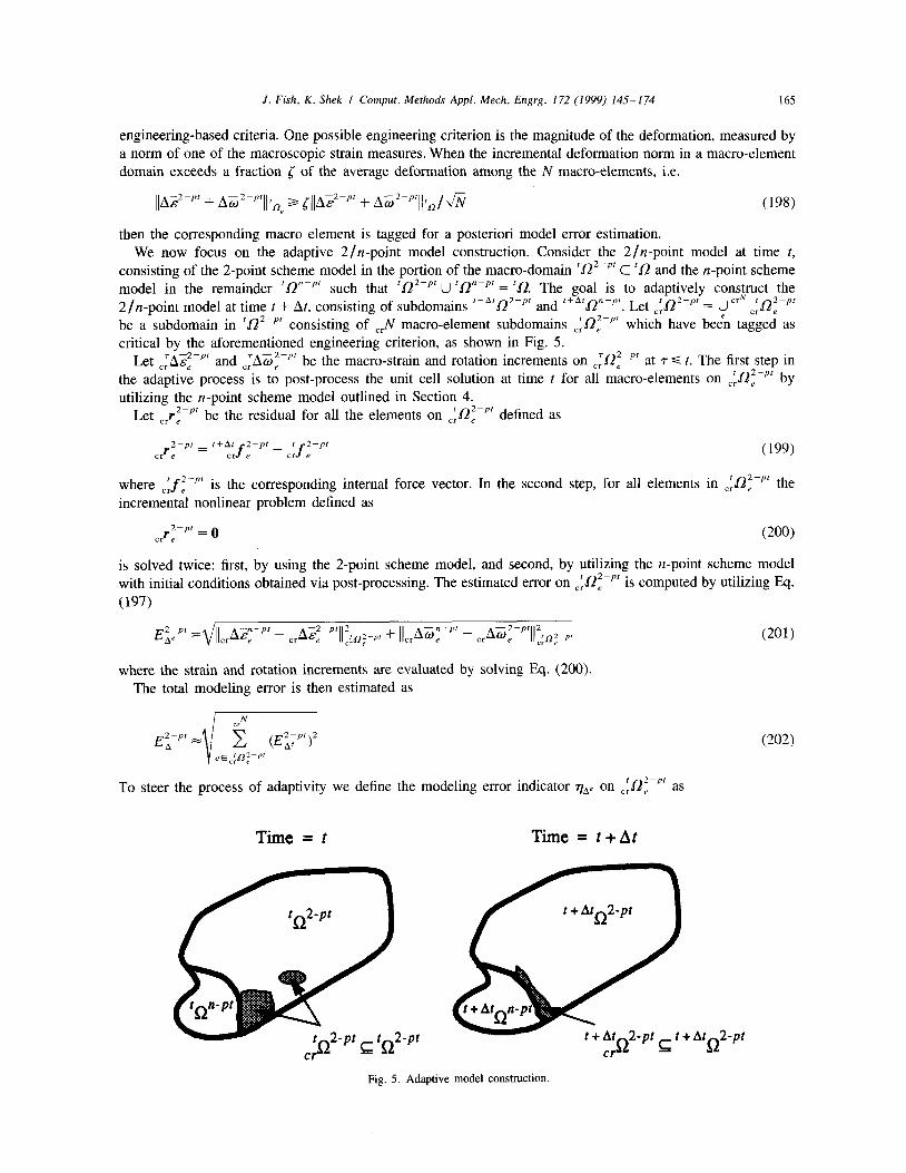
then the corresponding macro element is tagged for a posteriori model error estimation. We now focus on the adaptive 2/n-point model construction. Consider the 2/n-point model at time t,

consisting of the 2-point scheme model in the portion of the macro-domain r02-Pt C In and the n-point scheme model in the remainder ‘Finn-” such that r02-pr U tL2n-pr = ‘a. The goal is to adaptively cons$ruct the 2/n-point model at time t + At, consisting of subdomains f+Af02-p’ and t+A’finn-pr. Let c:ti2-p’ = U CT ,~~~~“’ be a subdomain in ‘anzmp’ consisting of c,N macro-element subdomains .$!-“’ which have been tagged as critical by the aforementioned engineering criterion, as shown in Fig. 5.

Let rAZ22-pr and c:ATi-p’ be the macro-strain and rotation increments on ,:Of-pr at r G t. The first step in the adzptivk process is to post-process the unit cell solution at time t for all macro-elements on ,:&-Pf by utilizing the n-point scheme model outlined in Section 4.

Let J:-~’ be the residual for all the elements on ,#-” defined as

2--pt- t+Ar 2--pf- f 2-e - .fe ,,f 7’ (199)

where ,,f e ’ *-” is the corresponding internal force vector. In the second step, for all elements in c$!~-Pt the incremental nonlinear problem defined as

2-PC - art! -0 @W

is solved twice: first, by using the 2-point scheme model, and second, by utilizing the n-point scheme model with initial conditions obtained via post-processing. The estimated error on cT ‘a:-” is computed by utilizing Eq. (197)

where the strain and rotation increments are evaluated by solving Eq. (200) The total modeling error is then estimated as

EA *-Pi z c (E;Fpt)*

eE,p-P'

To steer the process of adaptivity we define the modeling error indicator rl,, on ,:@“’ as

(202)

Time = t Time = t+At

Fig. 5. Adaptive model construction.

166 J. Fish, K. Shek I Comput. Methods Appl. Mech. Engrg. I72 (1999) 145 I74

where

py = llAZ2-p’ + AW2-pr~~~:12~-pr + (E;-“)*

2

(203)

(204)

py represents the average incremental deformation in a single element located in C$?-Pt. We replace the 2-point scheme model by the n-point scheme model for all the elements on C$-pt for which rla= 2 tol. A typical value for to1 is between 1% to 10% depends on the accuracy requirement.

6. Numerical experiments and discussion

Our numerical experimentation agenda consists of three examples. The first is used to validate our finite deformation plasticity formulation. The second and the third examples test the proposed adaptive 2/n-point scheme in a deformation pattern with large plastic zones dominated by matrix deformation as well as in a typical confined deformation pattern, where a small plastic zone is encompassed by an elastically deforming solid.

6.1. Uniform macro-strain loading

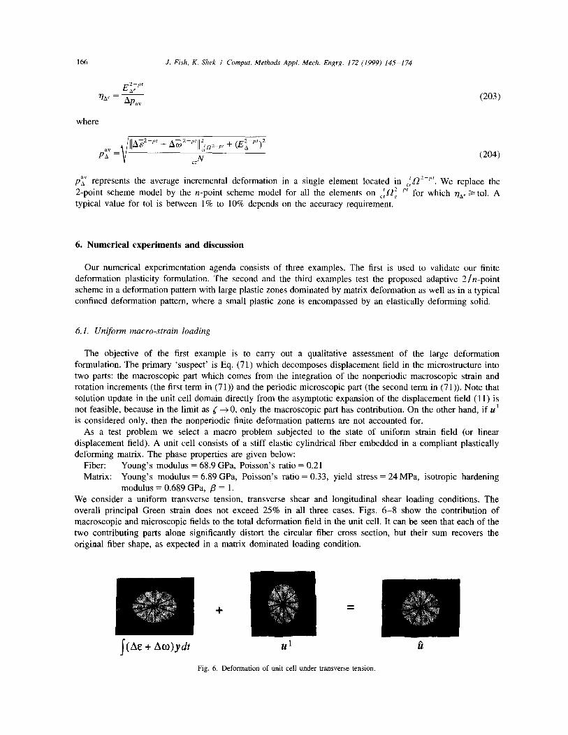
The objective of the first example is to carry out a qualitative assessment of the large deformation formulation. The primary ‘suspect’ is Eq. (71) which decomposes displacement field in the microstructure into two parts: the macroscopic part which comes from the integration of the nonperiodic macroscopic strain and rotation increments (the first term in (71)) and the periodic microscopic part (the second term in (71)). Note that solution update in the unit cell domain directly from the asymptotic expansion of the displacement field (11) is not feasible, because in the limit as 5 -+ 0, only the macroscopic part has contribution. On the other hand, if U’ is considered only, then the nonperiodic finite deformation patterns are not accounted for.

As a test problem we select a macro problem subjected to the state of uniform strain field (or linear displacement field). A unit cell consists of a stiff elastic cylindrical fiber embedded in a compliant plastically deforming matrix. The phase properties are given below:

Fiber: Young’s modulus = 68.9 GPa, Poisson’s ratio = 0.21 Matrix: Young’s modulus = 6.89 GPa, Poisson’s ratio = 0.33, yield stress = 24 MPa, isotropic hardening

modulus = 0.689 GPa, p = 1. We consider a uniform transverse tension, transverse shear and longitudinal shear loading conditions. The overall principal Green strain does not exceed 25% in all three cases. Figs. 6-8 show the contribution of macroscopic and microscopic fields to the total deformation field in the unit cell. It can be seen that each of the two contributing parts alone significantly distort the circular fiber cross section, but their sum recovers the original fiber shape, as expected in a matrix dominated loading condition.

J (AE + Aco)ydt

Fig. 6. Deformation of unit cell under transverse tension.

J. Fish, K. Shek I Comput. Methods Appl. Mech. Engrg. I72 (1999) 145- 174 167

J (AC + Ao)ydt z&l

Fig. 7. Deformation of unit cell under transverse shear.

J (A& + Ao)ydt u1

Fig. 8. Deformation of unit cell under longitudinal shear.

6.2. The 30 beam problem

To validate the computational models and adaptive strategies proposed we comprise a test case, where a significant portion of the structure is subjected to the matrix-dominated deformation in a load or stress control mode (as opposed to displacement control). This is a worse possible scenario in terms of accuracy for the 2-point scheme. The problem configuration is shown in Fig. 9. The macro problem is discretized with 5635 tetrahedral finite elements. The geometry and the mesh for the microstructure are the same as in the previous example. The fiber direction coincides with the beam’s longitudinal direction. In the region of length 1, from the fixed end tffe ‘oean? is sduje&ed tu ll-7e &rear ck7h7ii~iufl (wkzkfl is tie matrix-dotnirzated mode) w’neezs in fffe remainder of the problem domain, 1, length, the beam is in pure bending, which is a fiber-dominated mode of loading. The phase properties are summarized below:

Fiber: Young’s modulus = 31.92 GPa, Poisson’s ratio = 0.21 Matrix: Young’s modulus = 6.89 GPa, Poisson’s ratio = 0.33, yield stress = 24 MPa, isotropic hardening

modulus = 0.689 GPa, p = 1. The loading is applied in 15 load steps. The maximal vertical displacement at the free end is over one-third of the length of the beam and the stresses exceed the elastic limit in all macro-elements.

The problem is solved using the 2-point scheme with micro-history recovery, the adaptive 2/n-point scheme, and the n-point scheme for a comparison purpose. Fig. 10 shows the evolution of the normalized estimated local error in the vicinity of the fixed end as obtained with the 2-point scheme (Eq. (203)). It can be seen that the maximal normalized local error in the region dominated by matrix deformation is 40%. In a region dominated by the fiber deformation the enor dues not exceed 3%. Tk distribution of the kd principal stress error in the c~Stca1 unit ce11 idenoted by poin1 A in F& 10) a3 &lair& will2 the 2-prim dneme and mic70-‘niSqy postprocessing is shown in Fig. 11. It can be seen that the normalized error in the unit cell is of the same magnitude as the normalized local error in the macrostructure. Fig. 12 illustrates the evolution of the normalized l(ocA eno~ in tine miit~u~+~ri~Xint &s&-n& ukms tit a&&i-t 25 ~-~x+ii sckmk m&A. Tke. ma*mi ~~n-i-&Sii~& l(DC& enDT jS jes3 tim 5% an& tit nmdiixd %mix in ?!!t ah dh f&m% \kz %mi %d~ ?i% %kmi~ in Fig. \3.

we conclude that the adaptive 2/n-point scheme model outperforms the 2-point scheme model in terms of accuracy (0.8% maximal error as compared to 40%), and the n-point scheme model in terms of CPU time as it is 1 b zimes k&&7 >kQn &e n -pDb$ SEbZOX

168 J. Fish, K. Shek I Comput. Methods Appl. Mech. Engrg. 172 (1999) 145- 174

Fig. 9. Finite element mesh for the 3D beam problem.

Effective stress

Fig. 10. Distribution of the normalized local error with the 2-ooint model

Normalized error of effective stress Fig. Il. Effective stress and normalized error at point A with the 2-point model.

6.3. The nozzle jlap problem

For the final numerical example, we consider a typical aerospace component where only a small region experiences inelastic deformation. The finite element mesh describing the macrostructure of the Nozzle Flap is shown in Fig. 1. We consider two types of microstructures: (i) the fibrous unit cell (as in the previous example) and the plain weave fabric microstructure shown in Fig. 14. The fibrous unit cell contains 98 elements in the fiber domain and 2.53 elements in the matrix domain. The fiber volume fraction is 0.27. The plain weave microstructure has 370 elements in the fiber bundle and 1196 in the matrix domain. The bundle volume fraction is 0.25. The phase properties are:

Fiber, fiber bundle: Young’s modulus = 379.2 GPa, Poisson’s ratio = 0.21 Matrix: Young’s modulus = 68.9 GPa, Poisson’s ratio = 0.33, yield stress = 24 MPa, isotropic

hardening = 14 GPa, /5’ = 1. The Nozzle Flap is subjected to an aerodynamic force (simulated by a uniform pressure) on the back of the flap. We assume that the pin-eyes are rigid and a rotation is not allowed so that all the degrees of freedom on the

1. Fish, K. Shek / Comput. Methods Appi. Mech. Engrg. 172 (1999) 145-174 169

Fixed e

step 5

step 10

step 15

Fig. 12. Distribution of the normalized local error with the 2/n-point model.

Effective stress Normalized error of eft’ective stress Fig. 13. Effective stress and normalized error at point B with the 2/n-point model.

(a> Geometric model (b) Finite element mesh Fig. 14. Geometric model and FE mesh of the plain weave unit cell.


pin-eye surfaces are fixed. The loading takes the solution well into the inelastic region in the vicinity of the pins: 15% of elements experience inelastic deformation in the case of fibrous microstructure, and 29% in the case of plain weave.

The problem is analyzed using the adaptive 2/n-point scheme model. Fig. 15 shows that the 2-point scheme model yields the maximum normalized local error in the macrostructure below 1% (for the plain-weave microstructure). Hence, if the tolerance for switching from the 2-point scheme to the n-point scheme is higher than l%, adaptive strategy selects the 2-point scheme model in the entire macro-problem domain. The normalized local error in the unit cell located at Point C of Fig. 15 is 2.5% for fibrous microstructure and 6.5% for the plain weave, as shown in Figs. 16 and 17.

For the problem with the fibrous unit cell, the CPU time on a SPARC lo/51 is 30 s for the macroscopic analysis and 120 s for postprocessing a single point. For the plain-weave microstructure, the macroscopic analysis consumes 30 s, whereas post-processing takes 510 s per point. On the other hand, the n-point scheme consumes 7 h of CPU time for fibrous composite and over 55 h of CPU time for plain weave. Memory requirement ratios are approximately 1: 250 for the fibrous unit cell and 1: 1200 for the plain weave in favor of the 2/n-point scheme (or 2-point scheme).

step 1

step 3

step 5

step 7

Fig. 15. Nozzle flap problem/plain weave RVE: distribution of the normalized local error in the macrostructure as obtained with the 2-point model.


0.02 ,‘,<“,. :.

0.01

0.00

-0.01

-0.02

Effective stress Normalized error of effective stress Fig. 16. Effective stress and normalized error for fibrous unit cell as obtained with the 2-point model.

Effective stress Normalized error of effective stress Fig. 17. Effective stress and normalized error for plain weave unit cell as obtained with the 2-point model.

Acknowledgment

The authors gratefully acknowledge the support for this work by Air Force Office of Scientific Research under grant F49620-97- l-0090 and ARPA/ONR under grant N00014-92-J- 1779.

Appendix A. Derivation of a(~$’ - LU:‘)/~ AAcm’ in (96)

Consider Eq. (93):

g(r) - ‘I a;,?) = (Zijkl + AAcm) @Ljk,)-‘(tr(+;) - ‘S;:‘)

Taking the derivative of (A.l) with respect to AA’“’ yields

a ash’“’ (‘~1;) - CU;,~‘) = (I,,, + Ah’“’ M;,~~)-’

64.1)

04.2)


where the last term can be written as

and

The rotation %Li of phase r is defined in (77) as

%;l, = S,, + (S,, - + A”;;) -’ Awl’,’

The derivative of 8:: is calculated using the chain rule:

aiR;l, a%;; aA”“’ =-Py aAh’*’ aA@;; ddh’”

in which

Consequently, Eq. (A.4) can be expressed as

Similarly, we have

Taking derivative of (89) with respect to Ah’“’ yields

aAhw’“’ n (mm) ahh’“‘=D P pymn mnkl (

(*I c”kl - a:‘) + Ah’“’ -& (v;) - a;‘))

m

Substituting Eqs. (A.8)-(A.lO) into (A.3), and then inserting the result into (A.2), gives

(A. 10)

(A.ll)

(A.12)

(A.13)

64.3)

(A.4)

(A.3

(‘4.6)

67)

G-2

Appendix B. Consistent linearization of AZij and AWij

We derive the equations for A;,, and A4 consistent with the midpoint integration of rate of deformation and rotation. The left superscript t + At is omitted.

J. Fish, K. Shek I Comput. Methods Appl. Mech. Engrg. 172 (1999) 145- 174 173

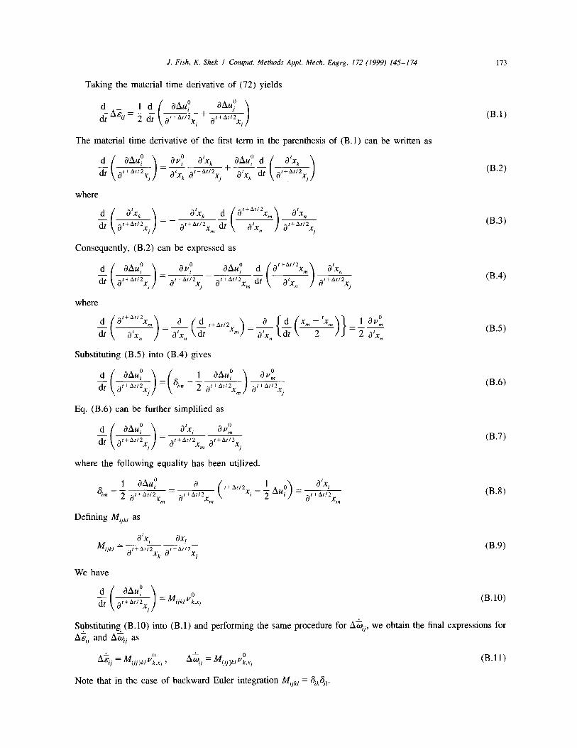
Taking the material time derivative of (72) yields

aAU; aAlL,! d'+A'/2x + dt+Ar/2xi

/

The material time derivative of the first term in the parenthesis of (B.l) can be written as

(B.1)

(B.2)

where

(B.3)

Consequently, (B.2) can be expressed as

(B.4)

where

~(a’~~~)=~(~~+A~~2x~)=~{~(xm~‘x..))=t~

Substituting (B.5) into (B.4) gives

(B.5)

03.6)

Eq. (B.6) can be further simplified as

afxi avi = ar+At12xm ar+Ar12xj

where the following equality has been utilized.

(B.7)

Defining M,,, as

f+At12 a’xi r+ArlZ

%I a xm (B.8)

Iv,,, = ak, ax,

a t+At/Zxk at+Ar12xj

We have

(B.9)

= Mijkl ‘L,x, (B.lO)

Substituting. (B. 10) into (B.l) and performing the same procedure for AGij, we obtain the final expressions for A$, and AZ, as

Note that in the case of backward Euler integration M,,, = S,,S,,.

174 .I. Fi.yh, K. Shek I Comput. Methods Appl. Mech. Engrg. 172 (1999) 14.5-174

References

[I] J. Aboudi, A continuum theory for fiber-reinforced elastic-viscoplastic composites, Int. J. Engrg. Sci. 20 (1982). [2] M.L. Accorsi and S. Nemat-Nasser, Bounds on the overall elastic and instantaneous elastoplastic moduli of periodic composites, Mech.

Mater. 5 (1986). [3] A. Benssousan, J.L. Lions and G. Papanicoulau, Asymptotic Analysis for Perodic Structure (North-Holland, 1978). [4] N.S. Bakhvalov and G.P. Panasenko, Homogenisation: Averaging Processes in Periodic Media (Kluwer Academic Publishers, 1989). [S] G.J. Dvorak, Transformation field analysis of inelastic composite materials, Proc. Roy. Sot. Lond., A437 (1992). [6] N. Fares and G.J. Dvorak, Large elastic-plastic deformations of fibrous metal matrix composites, J. Mech. Phys. Solids 39 (1991). [7] J. Fish, P. Nayak and M.H. Holmes, Microscale reduction error indicators and estimators for a periodic heterogeneous medium,

Comput. Mech. 14 (1994). [8] J. Fish, K. Shek, M. Pandheeradi and M.S. Shephard, Computational plasticity for composite structures based on mathematical

homogenization: theory and practice, Comput. Methods Appl. Mech. Engrg. 148 (1997) 53-73. 191 J. Fish and A. Wagiman, Multiscale finite element method for locally nonperiodic heterogeneous medium, Comput. Mech. 12 (1993).

[IO] S. Ghosh and S. Moorthy, Elastic-plastic analysis of arbitrary heterogeneous materials with the Voronoi cell finite element method, Comput. Methods Appl. Mech. Engrg. 121 (1995).

[I I] M. Gosz, B. Moran and J.D. Achenbach, Matrix cracking in transversely loaded fiber composites with compliant interphases, AMD-Vol. lSO/AD-Vol. 32, Damage Mechanics in Composites (ASME, 1992).

[ 121 J.M. Guedes, Nonlinear computational models for composite materials using homogenization, Ph.D. Thesis, University of Michigan, 1990.

[ 131 J.M. Guedes and N. Kikuchi, Preprocessing and postprocessing for materials based on the homogenization method with adaptive finite element methods, Comput. Methods Appl. Mech. Engrg. 83 (1990).

[ 141 J.O. Hallquist, NIKE2D: An implicit, finite deformation, finite element code for analyzing the static and dynamic response of two dimensional solids, University of California, Lawrence Livermore National Laboratory, Report UCID-19156, 1979.

[ 151 R. Hill, A self consistent mechanics of composite materials, J. Mech. Phys. Solids 13 (1965). [ 161 T.J.R. Hughes, Numerical implementation of constitutive models: rate-independent deviatoric plasticity, in: S. Nemat-Nasser, R.J.

Asaro and G.A. Hegemier, eds., Theoretical Foundation for Large Scale Computations for Nonlinear Material Behavior (Martinus Nijhoff Publishers, 1983).

[ 171 T.J.R. Hughes and J. Winget, Finite rotation effects in numerical integration of rate constitutive equations arising in large deformation analysis, Int. J. Numer. Methods Engrg. I5 (1980).

[ 181 S. Jansson, Homogenized nonlinear constitutive properties and local stress concentrations for composites with periodic internal structure, Int. J. Solids Struct. 29 (1992).

[ 191 A.L. Kalamkarov, Composite and Reinforced Elements of Construction (John Wiley and Sons, 1992). [20] E.H. Lee, R.L. Mallett and T.B. Wertheimer, Stress analysis for kinematic hardening in finite deformation plasticity, J. Appl. Mech. 105

(1983). [21] F. Lene and D. Leguillon, Homogenized constitutive law for a partially cohesive composite material, Int. J. Solids Struct. 18 (1982). [22] F. Lene, Damage constitutive relations for composite materials, Engrg. Fract. Mech. 25 (1986). [23] VM. Levin, Thermal expansion coefficients of heterogeneous materials, Mekhanika Tverdogo Tela, 2 (1967). [24] C.J. Lissenden and CT. Herakovich, Numerical modeling of damage development and viscoplasticity in metal matrix composites,

Comput. Methods Appl. Mech. Engrg. 126 (1995). [25] T. Mori and K. Tanaka, Average stress in matrix and average elastic energy of materials with misfitting inclusions, Acta Metallurg. 21

(1973). [26] H. Moulinec and P. Suquet, A fast numerical method for computing the linear and nonlinear properties of composites, C.R. Acad. Sci.

Paris II 318 (1994). [27] S. Nemat-Nasser, On finite plastic flow of crystalline and geomaterials, J. Appl. Mech. 105 (1983). [28] J.T. Oden and T.I. Zohdi, Analysis and adaptive modeling of highly heterogeneous elastic structures, TICAM Report 56, University of

Texas at Austm, 1996. [29] P. Ponte Castaneda, New variational principles in plasticity and their applications to composite materials, J. Mech. Phys. Solids 40

( 1992). [30] E. Sanchez-Palencia and A. Zaoui, Homogenization Techniques for Composite Media (Springer-Verlag, 1987). [X1] J.C. Simo and R.L. Taylor, Consistent tangent operators for rate-independent elastoplasticity, Comput. Methods Appl. Mech. Engrg. 48

(1985). [32] P.M. Suquet, Plasticite et homogeneisation, These de Doctorat d’ Etat, Universite Pierre et Marie Curie, Paris 6, 1982. [33] P.M. Suquet, Elements of homogenization for inelastic solid mechanics, in: E. Sanchez-Palencia and A. Zaoui, eds., Homogenization

Techniques for Composite Media (Springer-Verlag, 1987). [34] J.L. Teply and G.J. Dvorak, Bounds on overall instantaneous properties of elastic-plastic composites, J. Mech. Phys. Solids 36 (1988). [35] J.R. Willis, On methods for bounding the overall properties of nonlinear composites, J. Mech. Phys. Solids 39 (1991). [36] H. Zielger, A modification of Prager’s hardening rule, Quart. Appl. Math. 17 (1959). [37] T.I. Zohdi, J.T. Oden and G.J. Rodin, Hierarchical modeling of heterogeneous bodies, TICAM Report 21, University of Texas at

Austin, 1996.

finite deformation plasticity for composite structures: computational models and adaptive strategies

Documents