finite di erence models: one dimensionweb.pdx.edu/~chulbe/courses/modearthsys/lab6/lab6.pdfchapter 6...

Chapter 6

Finite difference models: onedimension

6.1 overview

Our goal in building numerical models is to represent differential equations in a computationallymanageable way. A large class of numerical schemes, including our initial value models of chapter3, do so using finite difference representations of the derivative terms. The model domain isdivided into a set of discrete, typically uniform, intervals of the independent variable (or variables).Arithmetic differences of function evaluations at the nodes between those intervals are used toapproximate the derivatives of the function over those intervals.

6.2 the difference approximation

Finite difference techniques rely on the approximation of a derivative as the change (or difference)in the dependent variable over a small interval of the independent variable,

dy

dx≈ ∆y

∆x

Those approximations are written using a small set of difference operators. These operators arehandy, they can be used to write formulae to interpolate, differentiate, and integrate “data.” Thedata might in fact be a set of measurements or, as in the case of a numerical integration scheme,might be the values of the dependent variable in a differential equation. The operators may beused singly to approximate first derivatives or in combination to approximate derivatives of anyorder.

The following definitions for finite difference operators use a particular set of Greek letters toidentify the operators. Don’t get sidetracked by that. The symbols are just a convenient shorthand(and you may find different symbols used in different texts). The names for the operations are

93

94 CHAPTER 6. FINITE DIFFERENCE MODELS: ONE DIMENSION

universal and you should always be able to find formulas or strategies for their implementation inan appropriate reference book. This presentation uses the function name f(x).

6.2.1 Taylor Series

Our approximation of the derivatives begins with their representation using the Taylor series. Wehave experience with the forward looking step:

f (xj+1) = f (xj) + hf (1) (xj) +h2

2f (2) (xj) +

h3

6f (3) (xj) + . . . (6.1)

where h = xj+1 − xj is the interval over which we wish to approximate the derivative and thesuperscripts indicate the order of the derivative of f(x). Truncating after the first derivative andrearranging yields an approximation of the first derivative

f (1) (xj) ≈f (xj+1) − f (xj)

h(6.2)

The numerator (f (xj+1)− f (xj)) is called the first forward difference of the function at xj .

A backward looking series is written

f (xj−1) = f (xj) − hf (1) (xj) +h2

2f (2) (xj) −

h3

6f (3) (xj) − . . . (6.3)

6.2.2 differences

Although we didn’t call it such at the time, the first forward difference was used in the Eulersingle-step method for solving an initial value problem. The basic difference operations may beused in combination to create other differences, as in the double-interval central difference.

forward difference

∆ f(xj) = f(xj+1) − f(xj) (6.4)

backward difference

∇f(xj) = f(xj) − f(xj−1) (6.5)

single-interval central difference

δ f(xj) = f(xj+ 12) − f(xj− 1

2) (6.6)

6.2. THE DIFFERENCE APPROXIMATION 95

double-interval central difference

1

2{∆ f(xj)−∇f(xj)} =

1

2{f(xj+1) − f(xj−1)} (6.7)

The double interval, created by differencing the forward and backward differences at xj is attractivebecause nodes j+ 1

2 and j− 12 in the single-interval central difference are not in the set of xj where

j = {1 : N + 1} are whole numbers.

6.2.3 higher-order differences

Higher-order differences are created by repeated differences. For example, applying the first forwarddifference to a first forward difference of a function gives us the

second forward difference:

∆2f(xj) = ∆ {∆ f(xj)}

∆2 f(xj) = ∆ {f(xj+1) − f(xj)}

∆2 f(xj) = f(xj+2) − 2 f(xj+1) + f(xj) (6.8)

The superscript on ∆ indicates that the operation is to be performed twice.

Similarly, we can derive the expression for the second central difference:

δ2f(xj) = δ {δ f(xj)}

δ2 f(xj) = δ{f(xj+ 1

2) − f(xj− 1

2)}

δ2 f(xj) = f(xj+1) − 2 f(xj) + f(xj−1) (6.9)

There are many ways in which the differences may be combined, including inverses and fractionalvalues.


6.2.4 using difference operators to compute derivatives

Derivatives are produced by dividing a finite difference by the interval over which the difference iscomputed. .

The first derivative of f(x) can be represented using a double-interval central difference:

f (1)(xj) =f(xj+1) − f(xj−1)

2 h+ error (6.10)

The magnitude of the error is discussed in section (6.2.5).

The second derivative of f(x) can be represented using the second central difference operator:

f (2)(xj) =f(xj+1) − 2 f(xj) + f(xj−1)

h2+ error (6.11)

6.2.5 numerical error

Truncation of the Taylor series introduces error into the numerical scheme. The magnitude ofthat error can be determined according to the order of the first truncated term in the series. Forexample, the first order Taylor expansion used in the first forward difference of the continuousfunction f(x) is

f (x+ h) = f (x) + hf (1) (x) +h2

2f (2) (ξ)

in which ξ is an unknown number between x and x + h. The corresponding finite differenceexpression is

f (x+ h) − f (x)

h= f (1) (x) +

h

2f (2) (ξ)

in which we can see that the error in the approximation is proportional to h. Expressed moregenerally, this is

f (1) (x) =f (x+ h) − f (x)

h+ O(h) (6.12)

in whichO indicates the order of the error in the approximation. The exact value of the errorcannot be determined because the value of ξ is unknown.

The centered difference is made by subtracting a backward from a forward difference. Taylorexpansions for these two differences are

f (x+ h) = f (x) + hf (1) (x) +h2

2f (2) (x) +

h3

6f (3) (ξ+)

f (x− h) = f (x)− hf (1) (x) +h2

2f (2) (x) − h3

6f (3) (ξ−)

in which the subscript on ξ indicates the intervals on the x+ h and x− h sides of x. Subtractingand rearranging yields

f (1)(x) =f(x+ h)− f(x− h)

2h− f (3)(ξ+) + f (3)(ξ−)

12h2

6.3. GENERIC EXAMPLE 97

f (1)(x) f (2)(x)

numerical 12.25 30.00exact 12 30

Table 6.1: finite difference approximate and exact derivatives of x3; x = 2, h=0.5

which may be simplified using the intermediate value theorem from Calculus

f (1)(x) =f(x+ h)− f(x− h)

2h− f (3)(ξ)

6(h2) (6.13)

and we see that the centered difference approximation is second-order accurate. A happy turn ofevents.

The exact error due to the finite difference approximation may be evaluated for a function forwhich the exact solution is available. Consider the function

f(x) = x3

The exact and numerical approximations of the first and second derivatives are

f (1)(x) = 3x2 ≈ (x+ h)3 − (x− h)3

2h

f (2)(x) = 6x ≈ (x+ h)3 − 2 (x)3 + (x− h)3

h2

Example calculations of the approximate and exact derivatives are given in table (6.1).

6.3 generic example

6.3.1 discretization: writing the governing equation in a finite difference form

Consider the the general linear second-order differential equation:

Q (x)d2y

dx2+ R (x)

dy

dx+ S (x) y + T (x) = 0 (6.14)

Our goal is to write this equation in a form that can be solved numerically for the unknown values ofthe dependent variable, y, at specified values of the independent variable xj j = {1, 2, . . . , N,N+1}, where x1 and xN+1 are the boundaries of the model domain. The dependent variable (orderivatives thereof) is known at x1 and xN+1.

N is the number of intervals between the N + 1 nodes in the model domain.

The finite difference form of equation (6.14) is produced by replacing the first and second derivativeswith first and second central differences:


Q (xj)y(xj+1)− 2y(xj) + y(xj−1)

h2+R (xj)

y(xj+1)− y(xj−1)

2h+ S (xj) yj + T (xj) = 0 (6.15)

Simplifying the subscripts for clarity, Q(xj) ≡ Qj , equation (6.15) is written:

Qjyj+1 − 2yj + yj−1

h2+Rj

yj+1 − yj−1

2h+ Sjyj + Tj = 0 (6.16)

Rearranging equation (6.16) to group terms by node number for the dependent variable,

(Qjh2− Rj

2h

)yj−1 +

(Sj −

2Qjh2

)yj +

(Qjh2

+Rj2h

)yj+1 = −Tj (6.17)

Terms involving the dependent variable are grouped on the left-hand side of (6.17) and termsinvolving constants are grouped on the right-hand side of the equation.

It is worth noting that at the first and last unknown nodes, the derivative terms include knownvalues of the dependent variable. These are the boundary conditions. The first and last equationsin our system are:

(Q2

h2− R2

2h

)y1 +

(S2 −

2Q2

h2

)y2 +

(Q2

h2+R2

2h

)y3 = −T2 (6.18)

(QNh2

+RN2h

)yN+1 +

(QNh2− RN

2h

)yN−1 +

(SN −

2QNh2

)yN = −TN (6.19)

Equation (6.18) is the finite difference approximation of the governing differential equation at thefirst unknown node in the domain, j = 2 and so it includes the boundary value y1. Equation (6.19)is the approximation at the last unknown node, j = N and so it includes the boundary value yN+1.

6.3.2 linear alegebra representation of the system

The system of equations (6.17) that form the numerical solution to (6.14) over the range of x istridiagonal. That is, three nodes in the model domain, and thus three values of y appear in eachdiscretized equation and the y are sequential: (j, j− 1), (j, j), (j, j+ 1). The system can be written

Ay = b

in which the matrix A contains the coefficients of the dependent variables, the vector y representsthose variables, and the vector b contains coefficients that do not involve unknown values of thedependent variable. The matrix equation visualized:

6.3. GENERIC EXAMPLE 99

1a21 a22 a23

a32 a33 a34

ai,i−1 ai,i ai,i+1...

...aN−1,N−2 aN−1,N−1 aN−1,N

aN,N−1 aN,N aN,N+1

1

y1

y2

y3

yi......

yN−1

yNyN+1

=

b1b2b3bi......

bN−1

bNbN+1

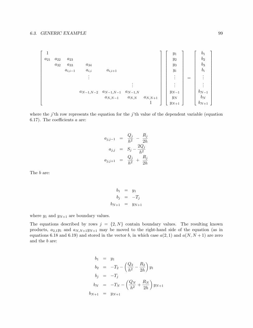
where the j’th row represents the equation for the j’th value of the dependent variable (equation6.17). The coefficients a are:

aj,j−1 =Qjh2− Rj

2h

aj,j = Sj −2Qjh2

aj,j+1 =Qjh2

+Rj2h

The b are:

b1 = y1

bj = −TjbN+1 = yN+1

where y1 and yN+1 are boundary values.

The equations described by rows j = {2, N} contain boundary values. The resulting knownproducts, a2,1y1 and aN,N+1yN+1 may be moved to the right-hand side of the equation (as inequations 6.18 and 6.19) and stored in the vector b, in which case a(2, 1) and a(N,N + 1) are zeroand the b are:

b1 = y1

b2 = −T2 −(Q2

h2− R2

2h

)y1

bj = −Tj

bN = −TN −(QNh2

+RN2h

)yN+1

bN+1 = yN+1


The matrix A and vector b are easily constructed using for loops. The only tricky part is treatingthe second and Nth rows differently than the other interior rows.

Once A and b are created, the y are found by solving y = A−1b. We will use Matlab’s backslashoperator to perform the calculation.

6.4 an example problem

6.4.1 a second-order linear differential equation with two boundary values

xd2y

dx2− 2

dy

dx+ 2 = 0 (6.20)

y (x = 0) = 0 and y (x = 1) = 0

The equation may be discretized using central differences:

xj

(yj+1 − 2yj + yj−1

∆x2

)− 2

(yj+1 − yj−1

2∆x

)+ 2 = 0 (6.21)

(xj

∆x2+

1

∆x

)yj−1 −

2xj∆x2

yj +

(xj

∆x2− 1

∆x

)yj+1 = −2 (6.22)

where ∆x represents the interval (or step) size.

The coefficients of equation (6.22) are used to build the known parts of the matrix equationrepresenting the system of equations that together represent the solution to equation (6.20) overthe model domain.

As before, we define N as the number of intervals between x1 = 0 and xN+1 = 1. The interval(step) size ∆x = (xN+1 − x1)/N .

The following formulae are used to generate the interior-row elements of A:

a(j, j − 1) =xj

∆x2+ 1

∆x

a(j, j) =2xj∆x2

a(j, j + 1) =xj

∆x2− 1

∆x

j = 2 . . . N

At this point, we have a decision to make. We can choose to keep the coefficients of the boundaryvalues in the matrix A (rows j = 2 and j = N) or we can choose to move the products of thecoefficients a(2, 1) and a(N,N+1) and the corresponding boundary values into the vector b. For ourcurrent purpose, the decision is trivial but for large problems with constant boundary conditions,it would make sense to store them at the start of the calculation and not create them repeatedlywithin a for loop.

6.4. AN EXAMPLE PROBLEM 101

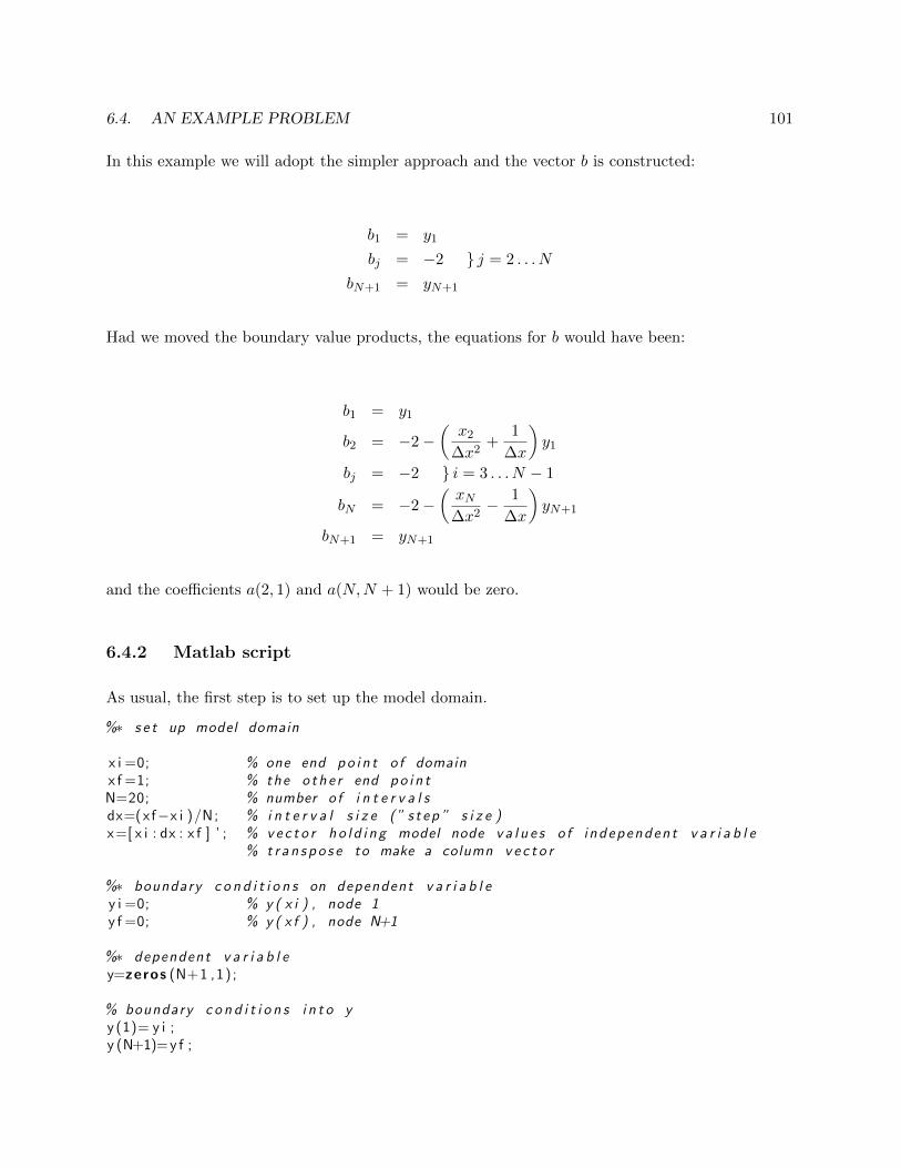
In this example we will adopt the simpler approach and the vector b is constructed:

b1 = y1

bj = −2 } j = 2 . . . N

bN+1 = yN+1

Had we moved the boundary value products, the equations for b would have been:

b1 = y1

b2 = −2−(x2

∆x2+

1

∆x

)y1

bj = −2 } i = 3 . . . N − 1

bN = −2−(xN∆x2

− 1

∆x

)yN+1

bN+1 = yN+1

and the coefficients a(2, 1) and a(N,N + 1) would be zero.

6.4.2 Matlab script

As usual, the first step is to set up the model domain.

%∗ s e t up model domain

x i =0; % one end po i n t o f domainx f =1; % the o th e r end po i n tN=20; % number o f i n t e r v a l sdx=( xf−x i )/N; % i n t e r v a l s i z e (” s t ep ” s i z e )x=[ x i : dx : x f ] ’ ; % ve c t o r h o l d i n g model node v a l u e s o f i ndependen t v a r i a b l e

% t r a n s p o s e to make a column v e c t o r

%∗ boundary c o n d i t i o n s on dependent v a r i a b l ey i =0; % y ( x i ) , node 1y f =0; % y ( x f ) , node N+1

%∗ dependent v a r i a b l ey=zeros (N+1 ,1) ;

% boundary c o n d i t i o n s i n t o yy (1)= y i ;y (N+1)= y f ;


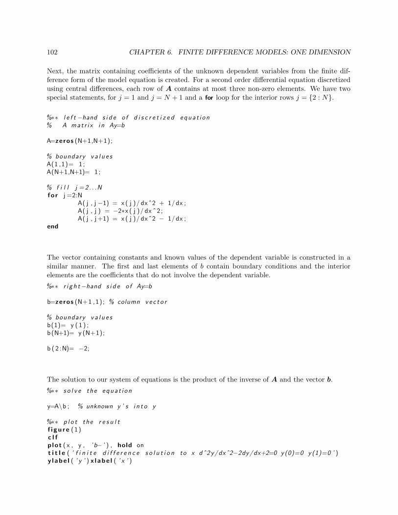
Next, the matrix containing coefficients of the unknown dependent variables from the finite dif-ference form of the model equation is created. For a second order differential equation discretizedusing central differences, each row of A contains at most three non-zero elements. We have twospecial statements, for j = 1 and j = N + 1 and a for loop for the interior rows j = {2 : N}.

%∗∗ l e f t −hand s i d e o f d i s c r e t i z e d equa t i on% A mat r i x i n Ay=b

A=zeros (N+1,N+1);

% boundary v a l u e sA(1 ,1)= 1 ;A(N+1,N+1)= 1 ;

% f i l l j =2 . . .Nf o r j =2:N

A( j , j −1) = x ( j )/ dx ˆ2 + 1/ dx ;A( j , j ) = −2∗x ( j )/ dx ˆ 2 ;A( j , j +1) = x ( j )/ dx ˆ2 − 1/ dx ;

end

The vector containing constants and known values of the dependent variable is constructed in asimilar manner. The first and last elements of b contain boundary conditions and the interiorelements are the coefficients that do not involve the dependent variable.

%∗∗ r i g h t−hand s i d e o f Ay=b

b=zeros (N+1 ,1) ; % column v e c t o r

% boundary v a l u e sb(1)= y ( 1 ) ;b (N+1)= y (N+1);

b ( 2 :N)= −2;

The solution to our system of equations is the product of the inverse of A and the vector b.

%∗∗ s o l v e the equa t i on

y=A\b ; % unknown y ’ s i n t o y

%∗∗ p l o t the r e s u l tf i g u r e ( 1 )c l fp lot ( x , y , ’ b− ’ ) , hold ont i t l e ( ’ f i n i t e d i f f e r e n c e s o l u t i o n to x dˆ2y/dxˆ2−2dy/dx+2=0 y (0)=0 y (1)=0 ’ )y l a b e l ( ’ y ’ ) x l a b e l ( ’ x ’ )

6.5. LAMINAR FLOW IN A CHANNEL (DERIVATION FOR EXERCISE 2) 103

zz + δz

x

x + δx

x

z

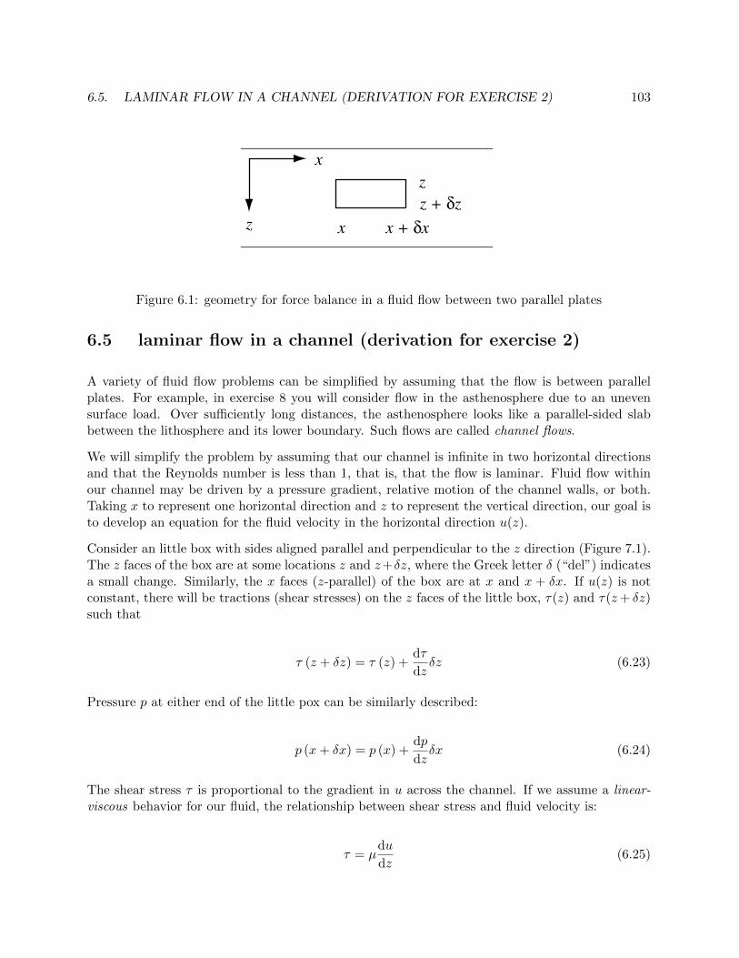
Figure 6.1: geometry for force balance in a fluid flow between two parallel plates

6.5 laminar flow in a channel (derivation for exercise 2)

A variety of fluid flow problems can be simplified by assuming that the flow is between parallelplates. For example, in exercise 8 you will consider flow in the asthenosphere due to an unevensurface load. Over sufficiently long distances, the asthenosphere looks like a parallel-sided slabbetween the lithosphere and its lower boundary. Such flows are called channel flows.

We will simplify the problem by assuming that our channel is infinite in two horizontal directionsand that the Reynolds number is less than 1, that is, that the flow is laminar. Fluid flow withinour channel may be driven by a pressure gradient, relative motion of the channel walls, or both.Taking x to represent one horizontal direction and z to represent the vertical direction, our goal isto develop an equation for the fluid velocity in the horizontal direction u(z).

Consider an little box with sides aligned parallel and perpendicular to the z direction (Figure 7.1).The z faces of the box are at some locations z and z+δz, where the Greek letter δ (“del”) indicatesa small change. Similarly, the x faces (z-parallel) of the box are at x and x + δx. If u(z) is notconstant, there will be tractions (shear stresses) on the z faces of the little box, τ(z) and τ(z+ δz)such that

τ (z + δz) = τ (z) +dτ

dzδz (6.23)

Pressure p at either end of the little pox can be similarly described:

p (x+ δx) = p (x) +dp

dzδx (6.24)

The shear stress τ is proportional to the gradient in u across the channel. If we assume a linear-viscous behavior for our fluid, the relationship between shear stress and fluid velocity is:

τ = µdu

dz(6.25)


where µ represents the viscosity of the fluid. This expression can be used, along with Newton’sSecond Law of motion, to derive an equation for u.

Newton’s Second Law of motion states that the sum of forces acting on an object must equal theproduct of the object’s mass and acceleration. In our laminar flow case, the acceleration must bezero, and we can use Newton’s Law to write a force balance equation for our little box within thefluid flow. The z faces experience shear forces

(τ (z) +

dτ

dzδz

)δx

and

−τ (z) δx

The x faces experience normal forces

p (x) δz

and

−(p (x) +

dp

dxδx

)δz

The force balance is thus:

∑F = 0

dτ

dzδzδx− dp

dxδxδz = 0

dτ

dz=

dp

dx(6.26)

Substituting (6.25) into (6.26),

d

dz

(µ

du

dz

)=

dp

dx(6.27)

and if µ is uniform,

µd2u

dz2=

dp

dx(6.28)

Equation (6.28) can be solved numericaly or exactly with appropriate boundary conditions on u.

6.6. EXERCISES 105

6.6 exercises

1. Derive the expression for the second backward difference. Write out all your steps.

2. The error associated with various approximations can be investigated by comparing finitedifference solutions with exact solutions for simple functions. Consider the function

f(x) = sin(x)

Using x = 1 and h = 0.1, show that a centered difference yields a better approximation of thefirst derivative f (1)(x) than does a forward difference. To do this, you will need to computethe local error at x = 1.

3. Consider a vector x that represents an independent variable and a second vector y thatrepresents a dependent variable that we believe to be a function of x. Here’s a bit of codethat could be used to calculate the first forward difference of y, assuming you are given someset of x and y:

% f i r s t f o rwa rd d i f f e r e n c e o f y w i th r e s p e c t to x

N=length ( y )−1;h=x (2)−x ( 1 ) ;

% f i r s t f o rwa rd d i f f e r e n c ef f d=zeros ( 1 , N ) ;

f o r n=1:Nf f d ( n)=( y ( n+1) − y ( n ) ) / h ;

end

f i g u r e ( 1 )c l fp lot ( ( x ( 1 :N)+x ( 2 :N+1))/2 , f f d , ’ r− ’ )

(a) Why is the dimension of ffd in the example code length(y)−1?

(b) Write a script or collection of functions that will accept any size x and y vectors (youwill need to measure the length of x and then use that dimension to create whateverother variables are necessary), and will calculate derivatives using the:

i. first backward difference of y with respect to x

ii. centered difference of y with respect to x

iii. second centered difference of y with respect to x

4. Two data files, testdat .mat and testdat2 .mat are available via ftp from the class website.Download the files. Each file contains two arrays, x and y, and x and y2. Use your collectionof scripts to compute the first derivative using forward, backward, and centered differences.Plot your results.


(a) Make a plot that compares the first forward difference and centered difference for thedata in testdat .mat.

(b) Make the same comparison for the data in testdat2 .mat. Why are the two derivativesdifferent for this data set but not for the data set in exercise 4a?

5. Implement the Matlab script in section 6.4. Try several domain resolutions. Turn in afigure showing solutions to the equation for three different resolutions.

6. Consider the equation

4d2y

dx2+

dy

dx= 0 (6.29)

(a) Write the equation in finite difference form.

(b) Write a Matlab script to solve the equation with the boundary values y(x = 0) = 0and y(x = 10) = 1. Plot your result.

7. Consider the equationd2y

dx2+ 2

dy

dx+ y = 0 (6.30)

(a) Write the equation in finite difference form.

(b) Write a Matlab script to solve the equation with the boundary values y(x = 0) = 1and y(x = 1) = 3. Plot your result.

8. The one-dimensional, non-turbulent flow of a viscous fluid in a channel is described by equa-tion (6.28). The fluid flow may be driven by a pressure gradient dp/dx, by motion of one ofthe channel boundaries with magnitude u, or both.

Suppose you want to use this equation to investigate the response of the asthenosphere toa change in the growth rate of a mid-ocean ridge. If the ridge growth rate has been steadyfor some time, then it is likely to be in isostatic equilibrium, and it does not drive a flowin the asthenosphere. However, if the ridge growth rate changes, the extra (or missing),uncompensated, thickness of ocean crust increases (or decreases) the pressure under theridge relative to the pressure at an equal depth at some distance from the ridge and theasthenosphere must adjust in order to return the system to isostatic equilibrium. Thatis, according to the hypothesis, an asthenosphere flow is driven by a gradient in lithostaticpressure (the weight of the uncompensated overlying rock) associated with the growing ridge.The gradient is

dp

dx= ρg

dh

dx(6.31)

in which ρ represents the density of the asthenosphere, g represents the acceleration due togravity, and dh/dx represents the gradient in uncompensated oceanic crust thickness acrossthe ridge.

If we assume that the speed of the asthenosphere is zero at its upper and lower boundaries,the boundary conditions for (6.28) are u (z = 0) = u (z = h) = 0.

6.6. EXERCISES 107

coefficient value units

µ 4 x 1019 Pa sρ 3000 kg m−3

g 9.81 m s−2

Table 6.2: coefficients for asthenosphere flow problem

This model is simple but it gives us a chance to practice using an equation with some physicalmeaning and it is a base from which a more complete model could be built.

(a) The first step in building the numerical model for this exercise is to approximate thesecond derivative of u and use the result to discretize the governing equation. Re-writeequation (6.28) using central differences.

(b) Using the program written in section 6.4 as a guide, write a Matlab script to modelu(z) in a 200 km thick asthenosphere at a point along the flank of a growing mid-oceanridge where dh/dx = −5× 10−4. Use the coefficient values supplied in table (6.2).

Write out, by hand, the equations you will use to construct the matrix of coefficientsof the unknown u (the matrix A) and the vector of known values(b) and use them towrite a Matlab script that solves (6.28) for the boundary conditions and constantsgiven here. Plot the simulated u(z), orienting the axes in a way that makes sense in thecontext of the process under investigation. Turn in your script and the figure.

9. Suppose you wish to include motion of the oceanic crust in your model of asthenosphere flow.Explain how that would be accomplished in this model, implement the change, and producea figure using a crust displacement rate of 50 mm a−1.

finite di erence models: one dimensionweb.pdx.edu/~chulbe/courses/modearthsys/lab6/lab6.pdfchapter 6...

Documents