finite-difference solution of the compressible stability ... · pdf filefinite-difference...
TRANSCRIPT

NASA Contractor Report 3584
Finite-Difference Solution of the Compressible Stability Eigenvalue Problem
Mujeeb R. Malik
CONTRACT NAS l- 16572 JUNE 1982
https://ntrs.nasa.gov/search.jsp?R=19820020697 2018-04-28T19:52:36+00:00Z

TECH LIBRARY KAFB, NM
: ll~llllnl~llllHRlllllII 0062143
NASA Contractor Report 3584
Finite-Difference Solution of the Compressible Stability Eigenvalue Problem
Mujeeb R. Malik Systems and Applied Sciences Corporation Hampton, Virginia
Prepared for Langley Research Center under Contract NAS l- 16572
National Aeronautics and Space Administration
Scientific and Technical Information Office
1982


Table of Contents
Summary.....................
Section 1 - Introduction . . . . . . . . . . . .
Section 2 - Compressible Stability Equations . .
Section 3 - Finite-Difference Representation . .
Section 4 - Global Method . . . . . . . .
Section 5 - Local Eigenvalue Search . . .
Section 6 - Calculation of Group Velocity
Section 7 - Richardson Extrapolation . .
Section 8 - Conclusion ....... . .
Appendix I ............. . .
Appendix II ............ . .
References ............. . .
. . . .
. . . .
. . . .
. . . .
. . . .
. . . .
. . . .
. . . .
. .
. .
. .
. .
. .
. .
. .
. .
. .
. .
. .
. .
Page . . . 1
. . . 2
. . . 6
. . . 10
. . . 13
. . . 16
. . . 19
. . . 22
. . . 24
. . . 25
. . . 31
. . . 36
iii

List of Tables
Table 1 - Characteristics of the sample test cases on a 35O swept wing . . . . . . . . . . . . . . . . . 38
Table 2 - Timings for the global eigenvalue method (time given in seconds on a CYBER 175 computer). . . . 39
Table 3 - Timings for the local eigenvalue method . . . . 39
Table 4 - Effect of the initial guess on the convergence of the local eigenvalue method ,for case 3 using N = 80, (8th order system) . . . . . . . . . . . 40
Table 5 - Computed group velocities for cases 1-3 using N = 80, (8th order system) . . . . . . . . . . . 40
Table 6 - Richardson extrapolation of the most unstable eigenvalue for case 1 . . . . . . '. . . . - . . 41
Table 7 - Richardson extrapolation of the most unstable eigenvalue for case 2 . . . . . . . . . . . . . 42
Table 8 - Richardson extrapolation of the most unstable eigenvalue for case 3 . . . . . . . . . . . . . 43
Table 9 - Comparison of eigenvalues obtained using different orders of extrapolation . . . . . . . . . . . . 44
List of Figures
Figure 1 - A schematic of the staggard finite-difference grid...................... 45
Figure 2 - Complex disturbance amplitudes plotted versus Y for case 1, - real ---- imaginary. These results were obtained using N = 80 . . . . . . . 46
iv

SUMMARY
A compressible stability analysis computer code is
developed. The code uses a matrix finite-difference method
for local eigenvalue solution when a good guess for the
eigenvalue is available and is significantly more compu-
tationally efficient than the commonly used initial-value
approach. The local eigenvalue search procedure also re-
sults in eigenfunctions and, at little extra work, group
velocities. A globally convergent eigenvalue procedure is
also developed which may be used when no guess for the
eigenvalue is available. The global problem is formulated
in such a way that no unstable spurious modes appear so
that the method is suitable for use in a black-box stability
code. Sample stability calculations are presented for the
boundary layer profiles of an LFC swept wing.

SECTION 1 - INTRODUCTION
The stability properties of compressible laminar boundary
layers are particularly relevant to the phenomenon of laminar-
turbulent flow transition. Recently, interest in this problem
has increased because of applications to Laminar Flow Control
(LFC) technology. In such applications there is a need for
fast computer codes to perform efficient design calculations.
The computer code SALLY [l] was developed for this purpose.
It can perform optimized stability calculations for determin-
ing suction requirements for maintaining laminar flow over
swept wings. However, SALLY uses incompressible stability
theory so it solves the eigenvalue problem for the fourth-
order Orr-Sommerfeld differential equation.
The linear stability analysis of three-dimensional com-
pressible boundary layers involves solution of an eigenvalue
problem for an eighth order system of differential equations.
In the case of two-dimensional boundary layers or in the
absence of dissipation in three-dimensional flow, the eighth-
order system reduces to sixth order.
The basic equations for the linear stability analysis of
parallel-flow compressible boundary layers are derived using
the Sam11 disturbance theory. Infinitesimal disturbances of
sinusoidal form are imposed on the steady boundary layer flow
and substituded in the compressilbe Navier-Stokes equations.

Assuming that the mean flow is locally parallel, a set of
five ordinary differential equations is obtained. Of these,
there are three second order momentum equations, one second
order energy equation and one first order continuity equation.
Following Lin [2-41 (his work involved only sixth order
system), this system is reduced to a set of eight first
order ordinary differential equations making the system
amenable to initial-value numerical integration procedures.
All previous numerical investigations of compressible
flow stability [5-101 make use of the initial value approach
for the solution of this system of eight first-order equa-
tions (or the reduced system of six first-order equations).
In these studies, the integration is started at a boundary
(usually the free stream boundary since the asymptotic solu-
tion of the stability equations provides initial values for
starting the integration) and marched to the other boundary
(solid wall) typically using a Runge-Kutta integration pro-
cedure. Four linearly independent solutions are sought
by means of this integration. The difficulty encountered
in this scheme is that a straight-forward integration fails
to produce four independent solutions because of parasitic
error growth. This difficulty is usually overcome by an
orthonormalization technique [see, e.g., 111. Upon obtaining
four accurate linearly independent solutions, linear combina-
tions are formed to satisfy all but one boundary condition
at the wall (the boundary towards which the equations are
marched). The remaining boundary condition is satisfied only
3

when the eigenvalue condition is satisfied. It is normally
imposed iteratively using a Newton-Raphson procedure which
results in the desired eigenvalue.
These initial-value methods to solve the compressible
stability equations are often computationally slow and thus
inefficient if used in a black-box stability code. Further-
more, the initial-value methods require a good guess for the
eigenvalue which is usually not available when one encounters
a new problem. In such cases one can obtain eigenvalues using
a local search procedure only by trial and error, which is
neither elegant nor efficient.
In the present work a computer code is developed for the
compressible stability analysis of three-dimensional boundary
layers. The code includes two eigenvalue search procedures-
global (which is to be used when no guess is available) and
local (which is used when a good guess is available). The
stability equations are solved in their original (3 second-
order momentum equations, one second-order energy and one
first-order continuity equation) using a matrix finite-
difference-method. The reduction of the normal momentum
equation to a first order equation for pressure fluctuations
as done by Lees and Lin [2] is not done here since that re-
sults in unstable spurious modes when the problem is solved
using the global method (see below).

The finite-difference representation of the stability
equations results in a block-tridiagonal system of equations.
A generalized matrix eigenvalue problem is then set up and
solved using the complex LR algorithm [12] for global eigen-
value search. The local search is performed by inverting the
block-tridiagonal system using a block LU factorization to-
gether with inverse Rayleigh iteration for the eigenvalues
[12] in which the eigenvalue, eigenfunction and its adjoint
are obtained simultaneously. One can obtain the group ve-
locities which are needed in an eigenvalue optimization pro-
cedure [13] at little extra cost to the local eigenvalue
search. The procedure used in the present study for local
eigenvalue solution is significantly faster than the initial
value approach employed by previous investigators.
Some sample calculations are performed for the stability
analysis of compressible three-dimensional boundary layer
profiles obtained for a laminar flow control wing using the
boundary layer code developed by Kaups & Cebeci (see ref. [l]).
particular wing chosen is a 35O swept super-critical wing
with an 8 foot chord. The free stream Mach number is 0.89.
Mack [7] and Lekoudis [9] reported stability calculations
for the same wing using their stability codes. We have
chosen three stations on the wing which represent forward
and rearward crossflow instability regions and a midchord
streamwise instability region. Some of the relevant boundary
data is given in Table 1. More details on the wing and press-
ure and suction distributions are given in reference 171 and
[9]. 5

SECTION 2 - COMPRESSIBLE STABILITY EQUATIONS
Consider the stability of a three-dimensional locally-
parallel compressible boundary layer flow. Let us use a
Cartesian coordinate system XlY,Z in which the y-axis
is normal to the solid boundary and x,z are parallel to
it. (In the particular case of a wing, the x-axis will be
assumed to be in the direction of the normal chord and the
z-axis will be along the span.) If u,v,w are the X,YlZ components of the instantaneous velocity, respectively, and
p and T are instantaneous pressure and temperature,
then, assuming that the base flow is locally parallel,
U(X,Y,Zlt) = uo(y) + zi (y) el(ax+Bz-wt)
v(x,y,z,t) = G(y) e i(ax+Bz-wt)
w(x,y,x,t) = we(y) + G(y) e= (ax+l3z-wt)
P(x,y,z,t) = p(y) e i (ax+Bz-cot)
T(X,Yrzrt) = To(y) + ‘i (y) e=(ax+Bz-wt)
(1)
(2)
(3)
(4)
(5)
Here Uo,Wo and To represent the steady unperturbed boundary
layer and quantities with tildas denote complex disturbance
amplitudes.
Substituting Eqs. (l-5) into the compressible Navier-
Stokes equations, it can be shown that the linear parallel
disturbances satisfy the following system of ordinary differ-
ential equations:
6

(AD2+B~+c)$ =o (6)
where d is a five-element vector defined by
iaii + fG, +, j3, T, .G - Bi3 T (7)
Here A,B,C are 5 x 5 matrices, and DE a dy '
where y is the
normal boundary layer coordinate. The non-zero elements of
the matrices A,B,C are given in Appendix I.
The boundary conditions for Eq. (6) are
y = 0; $I1 = $I2 = o4 = Q5 = 0 (8)
Equations (6-8) constitute an eigenvalue problem for
the frequency w and wavenumbers a,6 . For a given Reynolds
number R, this eigenvalue problem provides a complex dispersion
relation of the form
w = w(a,B) (9)
relating the parameters a,@ and w which, in general, are all
complex. In our analysis we choose to use temporal stability
theory in which a,f3 are real and w is complex. It is thus
assumed that the wavelike disturbances have 'x and z com-
ponents of wave number cx and f3 , respectively, and have a
frequency wr = Re (w). It is further assumed that the dis-
turbances grow or decay only in time. They grow if
w. 1 = Im(w) > 0 and decay if wi< 0.
7

The selection of temporal theory results in a linear
eigenvalue problem for w so that global eigenvalue techniques
can be applied. It is possible to extend the global method
to the spatial problem for the compressible stability equa-
tions but the work involved and the computer resources re-
quired discourage any such attempt. It appears that the most
efficient way to automatically provide a guess for the local
solution of the spatial stability problem is to first solve
the temporal global problem and then obtain the spatial guess
using the group velocity transformations [14].
Equation (6) represents three second order momentum
equations, one second-order energy equation and one first
order continuity equation. It is possible to eliminate
pressure entirely between these equations and to reduce
the system to four second-order equations for velocity and
temperature fluctuations. This reduction may seem desirable
for the numerical integrations since the order of the matrix
will be reduced. However, the elimination of pressure makes
the equations singular and their solution becomes difficult
to obtain in a numerically stable way. Similarly, it is
possible to reduce the system of eight first-order equations
to a single eighth-order differential equation 1151, but
this too is computationally ill conditioned. Thus, the follow-
ing analysis is carried out in terms of five equations: three
second-order equations for streamwise and spanwise velocity and
for energy, one first-order equation for continuity and one
8

second order (but effectively first-order) equation for
the normal velocity component.
9

SECTION 3 - FINITE-DIFFERENCE REPRESENTATION
The governing system of equations (6) for compressible
flow is represented using a second order finite-difference
formula on a staggered mesh (see Figure 1).
First the boundary layer coordinate Y, O~Y~Y, is
mapped into the computational domain O<n<l by the alge- - -
braic mapping
n =9-Y L+Y (10)
where g=l+$ e
Here ye is the location of the edge of the boundary layer
and L is a scaling parameter chosen to optimize the accuracy
of the calculations. After some experience it has been found
that a good choice for L is L = 2yo where y, is the value
of Y at which the streamwise component of the mean velocity,
uO’ achieves l/2 its freestream value. In the present study
we choose y = 100. e However, a much smaller value of y,(=15)
can be chosen for the local method since the free stream
boundary conditions are imposed using the asymptotic solution.
The computational domain rl is divided into N equal inter-
vals and the second order equations are represented as
fl Aj dj+l -2L+LBl
Arl ’ 1 +
10

+ d2 [f3Bj
(j=l l---l N - 1) (11)
where 4. 3
is the value of $ at n =,j/N and has components
'k,j (k = 1,...,5). Also,
dl = 1, d2 = 0 except
dl = 0, d2 = 1 for the 6 component
of 6,
(g-?-l) 4 fl=-- g2L2
2 (g-T-l) 3
f2=--22 gL
(g-rl) 2 f3= gL
The first order continuity equation is represented as
f3 Bj++ 5, *+1 -6. Arl
' + c. ,+L q+1 = 0 2 2 (12)
(j = O,...,N - 1)
Equations (11'12) along with the 8 boundary conditions
(8) represent 5N+4 equations for 5N+4 unknowns. Since the
velocity and temperature disturbances are assumed to be
identically zero at the solid boundary (n = 0) the system
reduces to 5N equations for 5N unknowns when these boundary
conditions are applied. This is a block-tridiagonal system
11

of equations with 5 x 5 blocks which is solved using fully
pivoted LU factorization.
Inthe global method, the free-stream conditions (n = 1)
are that c$~=$~=c$~=c$~=O at n = 1. This results in a linear
eigenvalue problem for n. In the local method, asymptotic
behavior of $ as y + 00 is found from (6) (see appendix II).
This asymptotic behavior is used to obtain a free-stream
boundary condition of the form
(ED + F) $ = 0 (13)
that is applied at n = 1 on components $k(k=1,2,4,5).
12

9 SECTION 4 - GLOBAL METHOD
When no guess is available for the eigenvalue of .interest,
it is best to use a method that is globally convergent and nearly
guaranteed to converge to the eigenvalue. Such a method may
be based on algorithms for calculations of the eigenvalues
of a general complex matrix [12].
When the compressible stability equations (11-12) are for-
mulated as a matrix problem, they take the form
Ti$= wB$ (14)
where w is the eigenvalue and T is the discrete representation
of the eigenfunction. The eigenvalue is determined by the
determinant condition
Detl x - w El = 0 (15)
For the present problem, B is invertible so (15) may be
solved as
Detl E-1 x -wII= 0 (16)
which is the standard matrix eigenvalue problem, solvable by
LR methods [12].
One has to be very careful in formulating the eigenvalue
problem (14) using global methods to avoid the generation of
growing (unstable) modes that are not physically relevant.
These spurious unstable modes do not correspond to solutions
of the differential equation- as the spatial resolution used
to discretize the eigenfunction increases true modes of the
differential equation converge while spurious modes do not.
13

A clumsy way to distinguish spurious modes from true
modes is to change the spatial resolution and retain only
those modes that do not change appreciably. This is neither
efficient nor elegant.
A better way is to eliminate the spurious unstable modes
entirely. Spurious stable modes are still possible, but since
these stable modes are normally very stable, they are not of
much interest and can be easily disregarded without testing
their true nature. We shall now describe a technique for
eliminating the spurious unstable modes.
The idea is simply that the spurious unstable modes
would, if we used the same numerical method used for the
stability problem on an initial-value problem instead, cause
the unconditional instability of the numerical solution of
the initial-value problem. On the other hand, if we were
careful enough to use a numerical method for the stability
problem that was also numerically stable for the initial-
value problem, then no spurious unstable modes would exist.
Thus, one way to avoid spurious modes is to set up the
problem as one would for an initial value problem and to use
a finite-difference scheme for the eigenvalue analysis that
is consistent with the scheme for the initial-value problem.
This is the method used in the present study: no spurious
unstable modes appear in our calculations. In some initial
work on this problem, we followed Lees and Lin 121 by re-
ducing the second-order normal momentum equation to a first-
order equation for pressure using the continuity equation.
14

This gives three second-order equations (two momentum and
one energy equation) and two first-order equations (one for
pressure and another for normal velocity). When the matrix
eigenvalue problem is set up using this system of equations
by means of finite-differencing, several unstable spurious
modes appear.
When the eigenvalue problem (16) is solved using the
LR algorithm, the storage requirements are of O(K2) while
the computational work involved is of O(K3) where K = 5N for
the eighth order system of equations and K = 4N for the sixth-
order system. It can be seen that the global method is
relatively expensive computationally so it should be only
used when no guess of the eigenvalue is available.
Some computer timings for the global method on a CYBER
175 computer are given in Table 2. All timings were obtained
using the internal clock and are averaged over the three test
cases listed in Table 1. Since the eigenvalue obtained by
the sixth-order system is not much different from that of
the eighth-order system, the use of the sixth-order system
for the global method is recommended.
15

SECTION 5 - LOCAL EIGENVALUE SEARCH
If a guess for the eigenvalue is available then one
can improve its value by a local method. One way to perform
the local analysis is to use a simple iterative'method to
find the eigenvalues of the matrix equation (15) that approxi-
mates the compressible stability equations. An effective and
efficient procedure for doing this is to use the inverse
Rayleigh iteration procedure [12]. The generalization of
this procedure to the compressible stability problem results
in the following algorithm
(A - Wk Bl -J (k+l) = g ; tk)
(A _ Wk E)T.~ (k+l) = sT $ tk)
Wk+l =
(17)
(18)
(19)
The iteration cycle is started with a guessed eigenvalue
w o and by assuming any smooth functional distribution for the
eigenfunction q(O) and its adjoint J(O). In an integration
of stability characteristics across a wing J(O) and J(O) may
be chosen as the eigenfunction and adjoint from the previous
station.
At the end of each iteration cycle k the eigenfunction
and its adjoint are normalized so that
16

(20)
The algorithm (17-20) has a rapid (cubic) rate of con-
vergence. The error satisfies Wk+l- w = 0 ( (w,-w) 3).
We solve the block-tridiagonal form of Eq. (17) by
using a fully pivoted LU method, in which case the same LU
factorization applies to the solution of the adjoint problem
(18).
In practice it is not necessary (rather, not recommended)
to update the eigenvalue approximation uk after each
iteration to the eigenfunction and its adjoint using (17-18).
We have found it to be most efficient to iterate (17-18)
approximately 4-10 times while keeping tik fixed (and,
therefore, using the same LU factorization of z-wkg). Once
the eigenfunction is refined less than 5 iterations are
required for a fixed ak. Generally, only two outer itera-
tions [LU factorizations and applications of (19) to update
Wk to Wk+ll are required to converge to an eigenvalue. Some
data on the speed of the local eigenvalue solution is given
in Table 3. The time reported also includes the calcula-
tion of group velocity. Since the eigenfunction and its
adjoint are available as a result of local eigenvalue search,
it costs little extra work to compute group velocity (see be-
low).
17

To show the sensitivity of the local method to the
initial guess some sample calculations are made and re-
ported in Table 4. The converged eigenfunction distribu-
tions vs y for case 1 using 80 points are plotted in
Figure 2.
18

SECTION 6 - CALCULATION OF GROUP VEJOCITY
The group velocity is of importance in relating the
results of spatial and temporal stability theory and in
several optimization problems [13]. In a layered flow
with three-dimensional disturbances having wavevector
(cl,f3) and frequency w(a,B) , the group velocity Gg is'
;: = (2% g
3.S) aa 1 af3 (23.1
One way to compute the group velocity is simply to
compute the frequency w for several nearby values of a,B
and then use finite-difference approximations to f g'
How-
ever, this procedure is not very efficient.
A much better way to compute the group velocity is
to first write the compressible stability equations for
three dimensional disturbances in the form
L(a,B,w(a,B))$ = 0
Taking the derivative of (22) with respect to c1 gives
(22)
(23)
Taking the inner product of (23) with the adjoint $ of the
eigenfunction & gives
(24)
19

since (5 L?;6/ac,) = (LT$ I I az/aa) = 0 . There is a similar afd expression fOr,a. Note that the inner product in (24) is
the usual L 2 vector inner product:
(1,~) =. ~ fi g i (25)
i=l
It is not necessary to use either the adjoint eigenfunction
of the differential equations (6) or the inner product
Jf(y)g(y)dy;$ is the adjoint of $ with respect to the
simple discrete inner product (25) and suffices to annihilate
the term a$/aa in (23).
The computation of the group velocity using (24) re-
quires only the calculation of aL/aa $(and aL/af3 6) since
L 3, awaw 4 are available from the local eigenvalue itera-
tions.
In Table 5, group velocities calculated by the present
method for the three test cases are compared with those cal-
culated by central differencing:
aw wj+l-wjAl
aa =a j j+l'"j-1 (26)
au wj+l-wj-l T& j = Bj+lmBj-l
which required four extra eigenvalue calculations so the
cost of determining group velocity was four times the cost
of the eigenvalue search. Using the present method, group
20

velocity can be obtained at less than 10% of the cost,of.the
eigenvalue search.
21

SECTION 7 - RICHARDSON EXTRAPOLATION
The finite difference method presented above is only
second order accurate. However, the accuracy of the eigen-
value (and the group velocity) obtained by this procedure
can be enchanced by Richardson extrapolation to the limit
An = l/N -f 0 [15].
If
s(o) i = w(hi) (i = O,...m) (27)
where hi is the grid size and w is the eigenvalue computed
by a method with error of O(h2), then
s (j-1)
,W = ,(j-1) + i-l _ ,(j-1)
i i i+l
(h hi 2
) -1 i+j
(28)
Cj=l I...., m, i=O ,.....,m-j)
Cj) The resulting approximation S i has an error of order
O(hj+2 ) when appropriate sequences of grid sizes h. are used. 1 We present here eigenvalue calculations for different grids
(hi = ;I and their extrapolated values. The sequence of
hi chosin is that proposed by Bulirsch and Stoer [16].
Tables 6,7,8 give eigenvalue results for boundary layer
data cases 1,2 and 3, respectively.
It can be seen that an eigenvalue converged to 5 sig-
nificant digits is obtained as a result of the extrapolation
procedure. For most applications, an eigenvalue that has
converged to 3 significant digits should suffice. This is
22

achieved by extrapolating only between three eigenvalues
at N = 20, 40 and 60. For three point extrapolation, (28)
reduces to the following formula
22 2 = [hl-h2) /ho Iwo +
7 7 7 [(h;-h;W;]wl + [(ho 2-h$/h;]w2
22 2 N-yh2)/hol +
22 2 +I (ho-hl)/h21 (29)
It is our experience that a reasonable answer can be
obtained by this extrapolation formula using only 20, 30
and 40 points. Eigenvalues obtained using this set of
points are compared with the converged value using 20, 40,
60, 80, 120 and 160 points in Table 9. The eigenvalue
accurate to 3 significant digits is obtained in about 2
seconds of CYBER 175 time.
23

SECTION 8 - CONCLUSION
Efficient local and global eigenvalue methods' for the
stability analysis of plane-parallel three-dimensional corn-
pressible boundary layers have been developed. The computer
code that implements these matrix boundary-value methods is
significantly more efficient than previous codes based .on
initial-value methods and is suitable for a black-box sta-
bility analysis package. ,
24

APPENDIX I
The Stability Equations
25

The stability equations for three-dimensional compressible
boundary layers are written as in (6) :
(AD2+BD+C)$=0
where
and
d Drdy
Here u, c, c represent the complex amplitudes of the per-
turbation velocity in x, y, z directions,respectively and 3,
? are the perturbation amplitudes of pressure and temperature.
The disturbances are assumed to be of the form
?4Y) e i(ax + Bz - Ut)
where a,@ are x and z wave numbers,respectively and w is the
(complex) frequency.
The non-zero elements of 5x5 matrices A, B and C are given
by
All = 1
A22 = 1
A44 = 1
A55 = 1
26

B1l = duO
k q Ti
B12 = i(X-1) (a2 + B2)
B14 = dpO
tq (au; + Bw;)
B21 = i(X-1)/A
dvO B22 = t dTo TA
R B23 = - 1.I,x
B32 = 1
B41 = 2(y-1114~ + BW$(n2 + B2)
2 dlJ, B44 = c q T,
B45 = 2(y-1)M2 (5 ccxw; - 8U&(a2 + f32)
1 dpo B54 = “0 T (“wo - Bu;)
1 dl-lo B55 = ‘“0 iq T;,
51 = -[i+ (“Uo + BWo - w) + A(a2 + B2) I 00 R
'12 = -‘poTo T; (a2 + B2) 1
* x-2 dll, T’ "21 = = x1.1, dTo o
c22 = - [; TRX (cm0 + BWo - w) + (a2 + f32,/xl 00
27

i 1 d'o --_c ‘24 = X v. dTo
C31 = i T--
c32 = - <
c33 =iy M 2 (au0 -I- owe - w)
i c34 = - T
(“IJo + gw - WI 0
Ra S c42 = - [uoTo To - 2 i (y-1)M2 o(aU;1 + Bw;) 1
iR0 c43 = l-Jo
(y-l)M2 (au 0
+ BWo - WI
c44 = iRa
- 'p T (cNo + BW 0 - w) + (a2 + B2)
00
- (y-l) aM2 + dpO /2 *2
o q ("o +wo)
dl.l _ 1 d21-1, (T;)2 _ k $ ‘,’ ]
'o dT2 0
0
R ‘52 = - voTo
1 d2vo dpO
c54 = I-‘0 dT 2 T; (cxW; - au,, + * -
0 dTo 0
iR ‘55 = - [uoTo
(cm0 + BWo -,w) + a2 + B2) 1
Here subscript o refers to the unperturbed boundary layer
and primed quantities represent the derivative of the quantity.
with respect to the boundary layer coordinate y.
28
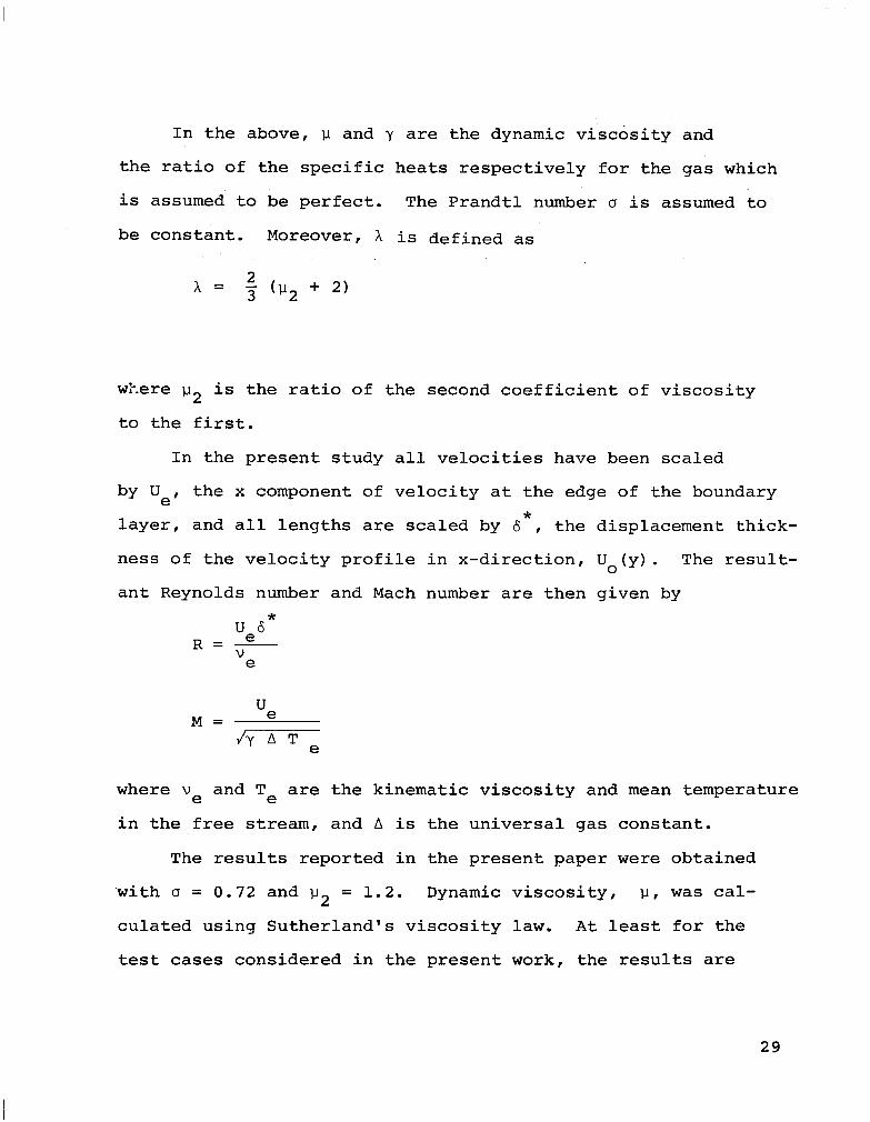
In the above, 1-1 and y are the dynamic viscosity and
the ratio of the specific heats respectively for the gas which
is assumed. to be perfect. The Prandtl number CI is assumed to
be constant. Moreover, X is defined as
wZere p 2 is the ratio of the second coefficient of viscosity
to the first.
In the present study all velocities have been scaled
by uet the x component of velocity at the edge of the boundary
layer, and all lengths are scaled by 6*, the displacement thick-
ness of the velocity profile in x-direction, Uo(y). The result-
ant Reynolds number and Mach number are then given by
U,S* R=-
V e
M= 'e Jy A T e
where v and T e e are the kinematic viscosity and mean temperature
in the free stream, and A is the universal gas constant.
The results reported in the present paper were obtained
with c = 0.72 and p2 = 1.2. Dynamic viscosity, p, was cal-
culated using Sutherland's viscosity law. At least for the
test cases considered in the present work, the results are
29

11, I I . . . . III I I ,11.1111.-.-.1 1..1..11 .,,,.,,..,, , . ..- -.... --.. ..-.- .-.-... --
not sensitive to the value of p2.
The special choice of $1 = cc6 + Bti and $5 = a% - 66
allows the eighth&order system of equations to reduce to
the sixth order for eigenvalue calculation if B45 is assumed
tC) be zero. This assumption implies the absence of dissipa-
tion.
30

APPENDIX II
BOUNDARY CONDITIONS
31

In the free stream (y 1 ye), the governing equations (6)
reduce to
D2el + B12 D Q2 + Cl1 +1 + Cl3 e3 - 0 (11-l)
D2@2 + B21 D $1 + B23 D $3 + C22 $2 = 0 (II-21
DQ2 + C31 $1 + C33 $3 + C34 $4 = 0 (II-31
D 2
@4,-+ C43 O3 + C44 44 = 0
D2Q5 + C55 4, = 0
(II-41
(II-51
where d D%-
The non-zero coefficients B.. and C.. are the same 13 13
as in appendix1 except that they are no more dependent on y. By
eliminating @,, the above equations can be written as
+ a D$, + e$l + f$, = 0 (II-61
D2q2 + b D$l + c Dq3 + g$, = C (II-71
D2$3 + d D$2 + s$~ + h+l = 0 (11-8)
where
and
a = B12 - c13'c33
b = (B21 - B23C31 J/(1 B23j
- - c33 c33
(II-91
C = (-'B23C34/C33)/(1- 22) c33
d = -c43/C33
e = Cl1 - c13 c31'c33
9 = c55
Equations (11-6) - (11-9) admit a general solution of
the form
8 Qi = C pj Zi(j) e
A j (Y-Y,) ;i=1,4
j=l (11-10)
where A. 3
are the eight characteristic roots of the coefficient
matrix of Equations (11-6) - (11-9) and Zi Cj) are the components
of the eight characteristic vectors z (3.
The asymptotic condition
Qi+O as y-f 00
is imposed by requiring that the arbitrary constants p. 3 vanish when
Re(Aj) > 0.
33
There are four A. 3
which satisfy this condition resulting
in four boundary conditions.
The roots Xj (j = I,... 6) can be obtained from the
characteristic equation (derived from Eqs. (11-6) - (11-8))
A4 + L2 x2 + L3 = 0
where
Ll = g +e+k-ab-cd
L2 = ke - hf + eg + kg - abk + bdf - ted + ahc
L3 = keg - ghf
2 Assuming that X =X , the above sixth order equation
reduces to the cubic equation
x3 + L1 x2 + L 2x+L =o 3
The roots of this cubic equation can be found as in
[173 and consequently six of the X.'s are known. The com- 7
ponents of the corresponding characteristic vectors are
tj) z1
= 1
d h? + de - ah ,W = 3
3 ka - fd + aAi
,W = 2
_ (h2 + e + f z$j))/a X. j 7
; j = I,6
The seventh and eighth characteristic root is simply
given as
x7 = (-q)+
X8 = - t-91 +
34

and the corresponding components of the characteristic
vectors are
z U3)= 1 4
All other components z Cj> are zero. i
Now, let
M =
where 8
$J. = c IrY
x ,W j=J
Pj j i ehj ('-'e) ;i=1,4
so
8 m. = 1 c ,W
'j i ex j (Y-Y,)
;i=1;8 j=l
where
N=
I &j) ’ x’, (3
ji,
;i=1,4
The arbitrary constants p. 3
are obtained by inverting
8x8 matrix N,
P =N -' M
The asymptotic boundary conditions require that P vanish
whenever Re(hj)>O. This results in four equations of the
form
(ED + F) I/J = 0
whereboth E and F are 4x4 matrices.
35

REFERENCES
1.
2.
3.
4.
5.
6.
7.
8.
9.
10.
11.
12.
13.
Srokowski, A. J. and Orszag, S. A., "Mass Flow Require- ments for LFC Wing Design," AIAA paper 77-1222, 1977.
Lees,.L. and Lin, C. C., "Investigation of the Stability of the Laminar Boundary Layer in a Compressible Fluid." NACA Technical Note No. 1115, 1946.
Lin, C. C., "The Theory of Hydrodynamic Stability." Cambridge University Press, London and New York, 1955.
Dunn, D. W. and Lin, C. C., "On the Stability of the Laminar Boundary Layer in a Compressible Fluid," J. Aeronautical Sciences 22, 455-477, 1955.
Brown, W. B., "Exact Solution of the Stability Equations for Laminar Boundary Layers in Compressible Flow." In Boundary Layer and Flow Control (G. V. Lachmann, ea.), Vol. 2, 1033-1048, Pergamon Press, London, 1961.
Mack, L. M., "Computation of the Stability of the Laminar Compressible Boundary Layer." In Methods in Computational Physics (B. Alder, ea.), Vol. 4, 247-299, Academic Press, New York, 1965.
Mack, L. M., "On the Stability of the Boundary Layer on a Transonic Swept Wing," AIAA Paper No. 79-0264, 1979.
Lees, L. and Reshotko, E., "Stability of the Compressible Laminar Boundary Layer," J. Fluid Mechanics 12, 555-590, - 1962.
Lekoudis, S. G., "Stability of Three-Dimensional Compress- ible Boundary Layers Over Swept Wings with Suction," AIAA Paper No. 79-0265, 1979.
El-Hady, N. M., "On the Stability of Three-Dimensional, Compressible Boundary Layers," AIAA Paper No. 80-1374, 1980.
Scott, M. R. and Watts, H. A., "Computational Solution of Linear Two-Point Boundary Value Problems Via Orthonormal- ization," SIAM J. Numerical Analysis 14, 40-70, 1977.
Wilkinson, J. H., "The Algebraic Eigenvalue Problem," Oxford, 1965.
Malik, M. R. and Orszag, S. A., "Comparison of Methods for Prediction of Transition by Stability Analysis," AIAA J. 18, 1485-1489, 1980.
36

14. Gaster, M., "A Note on the Relation Between Temporally- Increasing and Spatially-Increasing Disturbances in Hydrodynamic Stability," J. Fluid Mechanics, Vol. 14, 1962, p. 222-224.
15. Bender, C. M. and Orszag, S. A., "Advanced Mathematical Methods for Scientists and Engineers," McGraw-Hill, New York, 1978.
16. Bulirsch, R. and Stoer, J., "Numerical Treatment of Ordinary Differential Equations by Extrapolation Methods," Num. Math. 8, l-13, 1966.
17. Borofsky, S., "Elementary Theory of Equations", The Macmillan Company, New York, 1950.
37

Table l.-Characteristics of the sample test cases on a 35O swept wing
(chord, c = 8 ft).
Case Streamwise No. Location, R M a B et
x/c
1 0.001868 145 0.386 0.272117 -0.29181 51.96O
2 0.4639 3615 1.058 0.1153 0.0 26.93O
3 0.8921 1754 0.736 0.2432 -0.2654 34.80°
t Angle formed by the local potential flow vector with the x-axis.

Table 2. -Timings for the global eigenvalue method (time given in seconds on a
CYBER 175 computer).
N 8th order 6th order
system system
15 3.15 2.05
20 7.12 5.17
25 13.47 8.65 _. ..--.-~..
Table 3 Timings for the local eigenvalue method
N 8th order
system _-.- -
6th order system
20 0.61 0.40
1.14 0.77
80 2.22 1.52
39

Table 4. -Effect of the initial guess on the convergence of the local eigenvalue method for case 3 using N = 80, (8th-order system).
Tim& requiyer Initial guess for convergence
(0.011595,0.0023522)* 1.82
(0.01~,0.002) 2.38
(0.02,0.004) 2.95
(0.02,0.008) 3.10
(0.005,0.001) 3.11
(0.03,0.006) 3.50
(0.04,0.004) not converged
* equals the converged value
Table 5.- Computed group velocities-for cases l-3 using N = 80, (8th-order system).
w a Case Central Present
% Central Present
No. difference method difference method formula formula
1 (0.66039, (0.66036, -~ (0.73769 jO.73771, -0.00625) -0.00636) 0.01386) 0.01398)
2 (0.39893, (0.39876, (0.21884, (0.21867, 0.02105) 0.02063) -0.000987) -0.00155)
3 (0.53507, (0.53512, (0.44301, (0.44295, -0.05212) -0.05219) -0.04472) -0.04464)
40

Table 6. -Richardson extrapolation of the most unstable eigenvalue for case 1
Re(w) x 10
i N m= 0 1 2 3 4 5
1 20 -.2686117 -.2629801 -.2630158 -.2630098 -.2630087 -.2630100
2 40 -.2643880 -.2630118 -.2630102 -.2630087 -,2630099
3 60 -2.636234 -.2630106 -.2630089 0.2630099
4 80 -.2633553 -.2630093 -.2630097
5 120 -.2631631 -.2630096
6 160 -.2630959
Im(w) x 100
i N m= 0 1 2 3 4 5
1 20 .6073290 .6191717 .6186855 .6185509 .6186694 .6186523
2 40 .6162110 .6187395 . 6185593 .6186661 .6186525
3 60 .6176158 .6186043 .6186542 .6186534
4 80 .6180483 .6186418 .6186535
5 120 .6183780 .6186506
c 6 160 .6184972

iti Table 7.- Richardson extrapolation of the most unstable eigenvalue for case 2
Re(w) x 10 i N m= 0 1 2 3 4 5
1 20 .3940779 .3877680 .3889774 . 3888798 .3888478 .3888521
2 40 .3893454 .3888430 .3888859 . 3888486 . 3888520
3 60 .3890663 .3888751 .3888528 . 3888518
4 80 .3889827 .3888584 .3888519
5 120 .3889136 .3888535
6 160 .3888873
Im(w) x 100
i N m= 0 1 2 3 4 5
1 20 .0725901 .1230929 .1228928 .1227987 .1228500 .1228501
2 40 .1104672 .1229150 .1228046 .1228486 .1228501
3 60 .1173826 .1228322 .1228437 . 1228500
4 80 .1197668 .1228408 .1228491
5 120 .1214746 .1228470
6 160 .1220750

Table 8.-Richardson extrapolation of the most unstable eigenvalue for case 3
Re(w) x 10
i N m= 0 1 2 3 4 5
1 20 .1171532 .1158833 .1158746 .1158764 .1158752 .1158759
2 40 .1162008 .1158756 .1158763 .1158752 .1158759
3 60 .1160201 .1158761 .1158754 .1158758
4 80 .1159571 .1158756 .1158758
5 120 .1159118 .1158757
6 160 .1158960
Im(w) x 100 i N m= 0 1 2 3 4 5
1 20 .2200906 .2362895 .2362199 .2362203 .2362156 .2362186
2 40 .2322398 .2362276 .2362203 .2362158 .2362185
3 60 .2344553 .2362221 .2362163 .2362184
4 80 .2352283 .2362177 .2362181
5 120 .2357780 .2362180
6 160 .2359705
lh W

Table 9. -Comparison of eigenvalues obtained using different orders of extrapolation
Case No.
Three point Six point extrapolation extrapolation using N = 20, (see tables 30 and 40 6-8)
1 (-0.026303, (-0.026301, 0.0061848) 0.0061865)
2 ( 0.038889, ( 0.038885, 0.0012324) 0.0012285)
3 ( 0.011587, ( ,0.011587, 0.0023623) 0.0023621)
44

( FREE STREAM )
q=l 0 1
-----------l/2
I
j-l
(7) -----------j+l/2 j+ I
N-l e--e- ------N-l/2
Figure la- A SCHEMATIC OF THE STAGGARD FINITE-DIFFERENCE GRID
45

.6
.2 ii
.2
-.6
-1.0 I 0 2 4 6 8 IO
Y
.05 r
0 2 4 6 8 IO Y
-.02 -
-.04 -
-.06 I I I I I 0 2 4 6 8 IO
Y
.I0 r
.06 -
-.I0 _ I I 1 1 1 0 2 4 6 8 IO
Y
-.6 -
-1.0 I I I I I 0 2 4 6 8 IO
Y
Figure 2.- COMPLEX DISTURBANCE AMPLITUDES PLOTTED VERSUS Y FOR CASE 1; - REAL ---- IMAGINARY, THESE RESULTS WERE OBTAINED USING N = 80';
46

1. Report No. 2. Government Accession NO. 3. Recipient’s Catalog No.
NASA ~~-3584 1 4. Title and Subtitle
FINITE-DIFFERENCE SOLUTION OF THE COMPRESSIBLE STABILITY EIGENVALUE PROBLEM
- 5. Report Date
June 1982
I 6 Performing Organization Code
7. Author(s)
10. Work Unit No.
11. Contract or Grant No.
NASl-16572 13. Type of Report and Period Covered
Contractor Report 14. Sponsoring Agency Code
Mujeeb R. Malik
9. Performing Organization Name and Address
Systems & Applied Sciences Corporation 17 Research Drive Hampton, VA 23666
12. Sponsoring Agency Name and Address
National Aeronautics and Space Administration Washington, DC 20546
15. Supplementary Notes
Langley Technical Monitor: Julius Harris Final Report
16. Abstract
A compressible stability analysis computer code is developed. The code uses a matrix finite-difference method for local eigenvalue solution when a good guess for the eigenvalue is available and is significantly more computationally efficient than the commonly used initial-value approach. The local eigenvalue search procedure also results in eigenfunctions and, at little extra work, group velocities. A globally convergent eigenvalue procedure is also developed which may be used when no guess for the eigenvalue is available. The global problem is formulated in such a way that no unstable spurious modes appear so that the method is suitable for use in a black-box stability code. Sample stability calculations are presented for the boundary layer profiles of an LFC swept wing.
17. Key Words (Suggested by Author(s) )
Stability theory Transition Computational methods
__-~ -- 15. Distribution Statement
Unclassified - Unlimited
19. Security Classif. (of this report)
Unclassified 20. Security Classif. (of this page1
Unclassified
Subject Category 34 .~ ~
21. No. of Pages 22. Price
49 A03
For sale by the National Technical Information Service, Spinefield. Virginia 22161 NASA-Langley, 1982