FINITE ELEMENT ANALYSES OF PILE LOAD TESTS PERFORMED IN THE YORKTOWN FORMATION

NEWPORT NEWS, VIRGINIA

by

John Christos Daoulas

Thesis submitted to the Faculty of the Virginia Polytechnic Institute and State University

in partial fulfillment of the requirements for the degree of

MASTER OF SCIENCE

in

Civil Engineering

APPROVED:

------~ ------------------G. W. Clough, Chairman

J.M. Duncan

April 1988

Blacksburg, Virginia

FINITE ELEMENT ANALYSES OF PILE LOAD TESTS PERFORMED IN THE YORKTOWN FORMATION

NEWPORT NEWS, VIRGINIA

by

John Christos Daoulas

Committee Chairman: G.W. Clough Civil Engineering

(ABSTRACT)

The finite element method is used in determining

the load-capacity and behavior of a single concrete pile

modeled after full scale instrumented test piles which were

employed in the Tidewater area of Virginia. Specifically,

this report describes the subsurface conditions and full

scale pile tests that were performed during the des ign

phase of the foundation for the Land Level Shipbuilding

Facility in Newport News, Virginia. It also addresses the

testing conducted by the author to determine the material

properties required for finite element analyses, including:

soil sampling and in-situ tests within the Yorktown

formation; standard soil laboratory tests for index

properties and strength-deformation characteristics of the

soil along the pile perimeter and tip, plus interface tests

to evaluate soil strength-deformation characteristics along

the soil-pile interface. The data derived from the finite

element method of analysis is then compared with the load­

displacement and load-transfer data obtained from the full

scale instrumented pile load tests. The comparative

analysis shows favorable results leading to the conclusion

that the finite element method shows promise for use in the

design of deep foundations systems in the Tidewater area of

Virginia.

ACKNOWLEDGEMENTS

The author wishes to express his appreciation to

Dr. G.W. Clough, Professional Civil Engineer and Department

Head, and to Dr. T. Kuppusamy, Associate Professor of Civil

Engineering. Their guidance and assistance during the

course of this study were invaluable. Similarly, special

thanks are extended to Dr. R.E. Martin, Principal, Schnabel

Engineering Associates, P.C., of Richmond, Virginia for his

cooperation and assistance. In this connection, grateful

acknowledgement is

their sponsorship

hereby made to Schnabel Engineering for

of the test boring and Menard

pressuremeter tests conducted specifically for this study

program. In addition, I would like to thank the following

persons that were involved in the typing, drafting and

assembly of this manuscript: Diane Walden Ri tchie, Mary

Ann Jaramillo and Victoria Mitchell. Finally, I wish to

extend my sincere appreciation to my parents for their

encouragement and to my wife, Cheryl Lynn, for her patience

and support during all phases of this study effort.

iv

TABLE OF CONTENTS

ACKNOWLEDGEMENT

1.

2.

3 .

4.

INTRODUCTION

1.0 Background

1.1 Purpose

1.2 Scope of Study

SUBSURFACE CONDITIONS AND PILE LOAD TESTS

2.0 Data Sources

2.1 Foundation Features

2.2 Subsurface Conditions

2.3 Description of Pile Tests

2.4 Test Procedures

2.5 Pile Test Results

2.6 Analysis of Test Data

SOIL SAMPLING AND IN-SITU TESTING

3.0 Introduction

3.1 Soil Sampling and Standard Penetration Tests

3.2 Menard Pressuremeter Tests

SOIL LABORATORY TESTS

4.0 General

4.1 Basic Soil Properties and Classification

v

PAGE

iv

1

1

3

3

7

7

7

8

11

13

14

18

23

23

24

29

45

45

46

5.

6.

7.

4.2 Triaxial Testing of Soil Samples

4.3 SummaTY of Results

SOIL-CONCRETE INTERFACE TEST PROGRAM

5.0 Introduction

5.1 General Theory

5.2 Test Apparatus

5.3 Precast Interface Concrete Blocks

5.4 Soil Selection and Preparation

5.5 Interface Testing Procedures

5.6 Results and Analysis of Interface Tests

FINITE ELEMENT METHOD OF ANALYSIS

6.0 General

6.1 Finite Element Procedures

6.2 Application and Results

6.3 Analysis of Results

SUMMARY AND CONCLUSIONS

7.0 Summary

7.1 Findings

7.2 Conclusions

vi

PAGE

50

61

67

67

68

73

77

79

80

84

90

90

91

9 -,

100

116

116

117

122

REFERENCES

APPENDIX A - Pressuremeter Curves

APPENDIX B - Results of CU-Triaxia1 Tests Upper Yorktown Formation

APPENDIX C - Results of CD-Triaxial Tests Lower Yorktown Formation

APPENDIX D - Results of Soil-Concrete Interface Tests

VITA

vii

PAGE

124

126

133

137

141

148

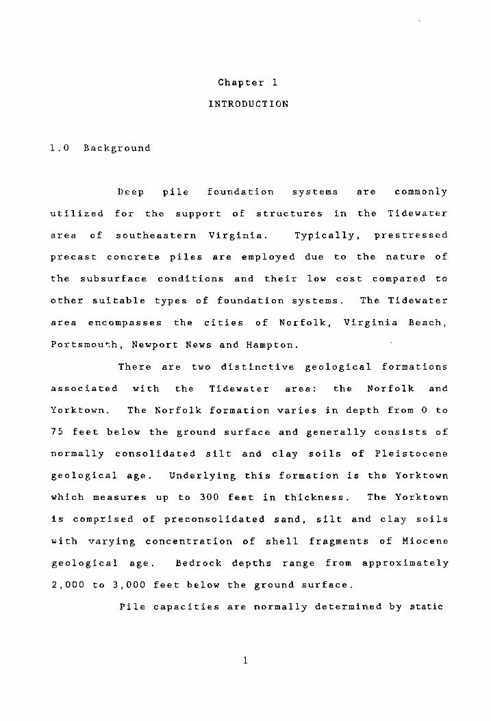
Chapter 1

INTRODUCTION

1.0 Background

Deep pile foundation systems are commonly

utilized for the support of structures in the Tidewater

area of southeastern Virginia. Typically, prestressed

precast concrete piles are employed due to the nature of

the subsurface conditions and their low cost compared to

other suitable types of foundation systems. The Tidewater

area encompasses the cities of Norfolk, Virginia Beach,

Portsmou~h, Newport News and Hampton.

There are two distinctive geological formations

associated with the Tidewater area: the Norfolk and

Yorktown. The Norfolk formation varies in depth from 0 to

75 feet below the ground surface and generally consists of

normally consolidated silt and clay soils of Pleistocene

geological age. Underlying this formation is the Yorktown

which measures up to 300 feet in thickness. The Yorktown

is comprised of preconsolidated sand, silt and clay soils

with varying concentration of shell fragments of Miocene

geological age. Bedrock depths range from approximately

2,000 to 3,000 feet below the ground surface.

Pile capacities are normally determined by static

1

2

and dynamic formulas. These methods, however t usually

provide conservative estimates of their actual load

capacity due to the nature and variation of the soil strata

that comprise the Yorktown Formation. The results of in-

situ tests, such as Standard Penetration and Menard

Pressuremeter, are adversely effected by the presence of

cemented shell fragments, development of excess pore water

pressure, and soil disturbance typically found to occur

within this Formation. Pile driving data used in dynamic

analysis has also been found to be effected by these

conditions. Consequently, in the past ten years,

correlation factors have been modified based on data from

full scale pile load tests to improve the design of deep

foundation systems based on static analyses.

This was done for the foundation system that

supports the Land Level Shipbuilding Facility at Newport

News, Virginia. During the design phase of the foundation,

various subsurface investigations and pile load tests were

conducted. These included the use of instrumented piles to

determine the mechanism and magnitude of support derived

from the Yorktown formation. The resultant data was then

used to develop new values for correlating the unit shaft

and base resistance of piles with Standard Penetration Test

data (14).

Although test data for piles embedded within the

Yorktown formation are useful, it generally cannot isolate

3

the effects of the following: in-situ stresses; soil

disturbance and induced stresses caused by pile driving;

variations in soil strength and soil-pile interface

properties; consolidation and negative skin friction plus

cyclic loading. The finite element method of analysis,

however t appears capable of incorporating many of these

factors. This method could therefore result in an improved

understanding of the load-deformation response of piles.

1.1 Purpose

The purpose of this study is to assess the

effectiveness of the finite element method for determining

the capacity and behavior of piles of deep foundation

systems in the Tidewater area of Virginia. In order to

accomplish the above obj ective, field and laboratory test

programs were undertaken to determine the engineering

parameters required for the finite element analysis. This

endeavor further permits an assessment to be made regarding

the feasibility of using the finite element method in lieu

of full scale pile tests for future design.

1.2 Scope of Study

The finite element method is used to ascertain

the behavior of a single concrete pile under various load

4

conditions to include ultimate load capacity; the pile is

modeled after instrumented piles utilized at the Land Level

Shipbuilding

characteristics

Facility.

of the soil

The stress-deformation

and soil-pile interface

properties are determined. The methods and tests for

developing the data required by the finite element method

include: soil sampling; Standard Penetration Tests;

standard laboratory tests for the determination of index

properties and stress-deformation characteristics; and

soil-structure interface testing to determine stress-

deformation characteristics of the soil along the soil-pile

interface. In addition, Menard pressuremeter tests are

performed to enhance the data base. The features of the

Shipbuilding Facility are discussed briefly followed by a

detailed description of the subsurface conditions and the

manner in which they were identified. An in-depth analysis

is made of the full scale pile load tests to include

delineating the procedures and tabulating the results.

Test incidents which affected results are also highlighted

since they have to be considered in the comparative

analysis with results derived from the finite element

method.

Although considerable subsurface soil data

resulted from the investigations conducted by Schnabel

Engineering, additional soil sampling and in-situ testing

at the site was performed to support the laboratory test

5

program established for this study. The

results of this effort are treated in

scope, types and

detail. Field

investigations included the following: split-spoon

sampling, Standard Penetration Tests; and Menard

pressuremeter tests. The apparatus and procedures are

addressed for each of these activities.

Standard soil laboratory tests were conducted to

establish the basic properties and classification of the

soils of the Yorktown formation. In addition, triaxial

tests were performed to develop data required in connection

with the finite element method. In this regard, the manner

of determining the hyperbolic soil model parameters for

soils along the pile perimeter are set forth in a step-by­

step procedure and the results summarized. Similarly,

laboratory tests were conducted to determine the stress­

deformation characteristics along the pile-soil interface.

This was accomplished by fabricating concrete blocks to

represent the pile surface and using a direct shear

apparatus that was appropriately modified for this phase of

the test program. The test procedures, sample preparation

and features of the apparatus are described in addition to

the results.

The foregoing elements provided the requisite

inputs for use of the finite element method of analysis.

Although no attempt

theory of this method,

is made to describe the operative

the steps that have been devised for

6

determining the ultimate bearing capacity of piles, their

load-deformation behavior and load-transfer characteristics

are addressed. The results achieved therefrom are then

analyzed in relation to those from the full-scale pile test

program.

The data generated from this study are reflected

in several graphs and tables incorporated within the report

and in the appendices. In the final section, the report is

summarized and pertinent findings and conclusions are

addressed.

Chapter 2

SUBSURFACE CONDITIONS AND PILE LOAD TESTS

2.0 Data Sources

Various reports prepared by Schnabel Engineering

Associates, P.C. were used for the topics that are covered

in the succeeding paragraphs. The specific topics include:

foundation features; the description of soils associated

with the strata of the Norfolk and Yorktown formations; and

pile test descriptions, procedures and results.

2.1 Foundation Features

In 1984, the Tenneco Company began construction

of a multi-million dollar Land Level Shipbuilding Facility

at the Newport News Shipbuilding and Dry Dock Company

located in Newport News, Virginia. The structure has plan

dimensions of approximately 600 by 1100 feet and was

designed to facilitate the construction of Navy ships and

submarines. The foundation design includes approximately

10,000 closely spaced, prestressed, precast square concrete

piles with a design capacity of 100 tons each. Parsons,

Brinckerhoff, Quade and Douglas, Inc. were the designers of

the structure to include the foundation system. Schnabel

Engineering Associates, P. C. t a Geotechnical engineering

7

8

consulting firm, located in Richmond, Virginia conducted

the subsurface investigation and testing program for the

project. Schnabel's activities included the conduct of

load tests with both instrumented and non-instrumented

piles in conjunction with their design effort regarding

pile type, length, spacing, and installation criteria.

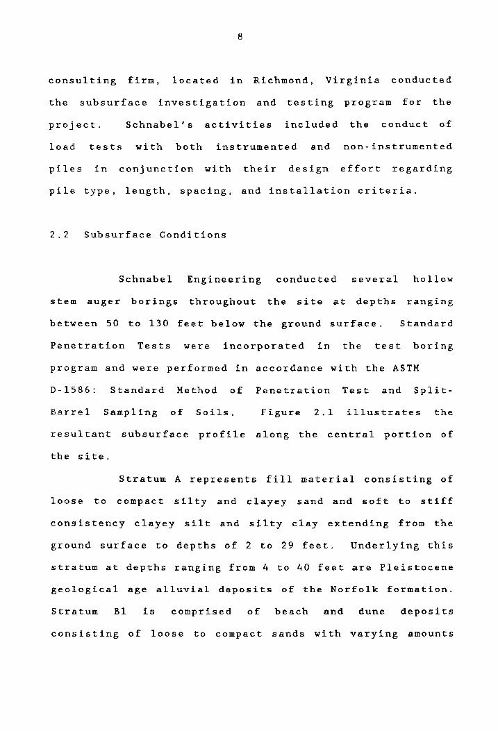
2.2 Subsurface Conditions

Schnabel Engineering conducted several hollow

stem auger borings throughout the site at depths ranging

between 50 to 130 feet below the ground surface. Standard

Penetration Tests were incorporated in the test boring

program and were performed in accordance with the ASTM

D-1586: Standard Method of Penetration Test and Split-

Barrel Sampling of Soils. Figure 2.1 illustrates the

resultant subsurface profile along the central portion of

the site.

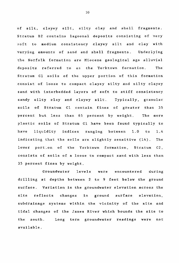
Stratum A represents fill material consisting of

loose to compact silty and clayey sand and soft to stiff

consistency clayey silt and silty clay extending from the

ground surface to depths of 2 to 29 feet. Underlying this

stratum at depths ranging from 4 to 40 feet are Pleistocene

geological age alluvial deposits of the Norfolk formation.

Stratum BI is comprised of beach and dune deposits

consisting of loose to compact sands with varying amounts

roo· 1-1 ------4 10 ~

EXISTING !U.J( HEAD GAD. SURFACE _ _ AND PUMP HOUSE ---£: ________ _----_

- A _------------------- 81 _------~~. --~ ~ -

.......,;- 8! _----~"".- ...--~------ ........ ----_ ....... S) e.

40

-- ",.".,-~ ................ ---- ---~ ...... ~ ~ ~ ...,..- ..... ...-.....-. ....... --- -- --- --.~ - --- ----~ - - ...-

to --

JIWD RIVER

Itt:1!Jd

..... t,tlllaO' \J!M:t I"I'«:}'

CI

SECTtON A-A

PLAN

FIGURE 2.1 SleSLRFACE PROFlLE

100

t()

GO

40

20

\0

10

of silt, clayey silt, silty clay and shell fragments.

Stratum B2 contains lagoonal deposits consisting of very

soft to medium consistency clayey silt and clay with

varying amounts of sand and shell fragments. Underlying

the Norfolk formation are Miocene geological age alluvial

deposits referred to as the Yorktown formation. The

Stratum Cl soils of the upper portion of this formation

consist of loose to compact clayey silty and silty clayey

sand with interbedded layers of soft to stiff consistency

sandy silty clay and clayey silt. Typically, granular

soils of Stratum Cl contain fines of greater than 35

percent but less than 65 percent by weight. The more

plastic soils of

have liquidity

Stratum CI have been found typically to

indices ranging between 1.0 to 1.4

indicating that the soils are slightly sensitive (14). The

lower port'on of the Yorktown formation, Stratum C2,

consists of soils of a loose to compact sand with less than

35 percent fines by weight.

Groundwater levels were encountered during

drilling at depths between 2 to 9 feet below the ground

surface. Variation in the groundwater elevation across the

site reflects changes in

subdrainage sys tems wi thin

ground surface

the vicini ty of the

elevation,

site and

tidal changes of the James River which bounds the site to

the south. Long term groundwater readings were not

available.

11

2.3 Description of Pile Tests

Six test piles, identified as TP-l through TP-6,

were installed at the site. All six were 14 inch square

prestressed, precast concrete piles. Test piles TP-l,

TP-2, TP-5 and TP-6 were 90 feet in length and were not

instrumented. Piles TP-3 and TP-4 were 70 feet in length

and were ins trumented wi th vibrating wire strain guages

embedded at intervals of 10 feet along their central axis.

Instrumentation was accomplished at the time the piles were

cast.

Piles TP-1, TP-2 and TP-3 were embedded

approximately 42 feet within Stratum Cl to depths of 55, 60

and 61 feet respectively below the ground surface. Piles

TP-4, TP-5 and TP-6 were embedded approximately 44 feet

within Strata Cl and C2 at depths of 58, 71 and 48 feet

respectively below the ground surface. All six test piles

were driven continuously to the required tip elevation

using a Vulcan 010 single acting air driven pile hammer

wi th an energy ra ting of 32,000 ft. -lbs. The location of

each of the six test piles are shown in Figure 2.2.

Piles TP-3, TP-4 and TP-5 were selected for load

tests which were performed in accordance with ASTM D-1143-

81: Piles Under Axial Compressive Loads. During

preparation for load testing of pile TP-4, settlement of

the load frame reaction cribbing resulted in preloading.

ElLK HEAD

... 130' ·1· 3m' ,. ~ 335 • ~ TP_& ~-2 . v 'T' T T

ASSEMBLY PLATEN NO. 9.5

~ ('\J

SH I PWAY NO. 9

TP-6 -~

SHIPWAY NO.8 1 tftTP-,

iN

BLDG. NO. 214 J I Blex;. NO. 213

-$- TEST PILE LOCATION

FIGURE 2.2 TEST PILE LOCATION PLAN, LANOLEVEL ' SHIPBUILDING FACILITY

....... N

13

In addition, during the test the electronic load cell

malfunctioned resulting in erroneous readings. Hence, the

load test was terminated at this juncture and the pile was

driven an additional 4.0 feet. After a period of 72 hours,

to allow for excess pore pressure dissipation and

thixotropic strength gain resulting from redriving, testing

of pile TP-4 was performed in accordance with ASTM D1143-

81.

2.4 Test Procedures

frame.

Loads were applied by jacking against a load

An electronic load cell positioned between the jack

head and reaction beam of the load frame was used to

monitor applied loads. Three dial guages mounted

independently of the load frame were used to measure

vertical movement of the test pile. These were checked

using an independent wire, mirror and rule system.

The procedures utilized for load testing of piles

TP-3 and TP-5 were as follows. The test pile was initially

loaded to twice the 100 ton design load in 25 ton

increments. Each load increment was maintained until the

rate of settlement was less than 0.01 inches in one hour or

for a period no longer than two hours. The 200 ton load

was held for a period of 15 hours and then unloaded in 50

ton increments to zero load. After a period of less than

14

one hour, the pile was reloaded to 200 tons in 50 ton

increments with each load held for 20 minutes. Loading

continued beyond 200 tons in 10 ton increments with a 20

minute hold until the pile failed to maintain the load or

to the maximum 300 ton capacity of the load frame reaction

system. The load application procedures described above

were also used for pile TP-4 except the pile was not

subjected to the unload-reload cycle. The load-settlement

curves for the applied load cycles are presented in Figure

2.3 for piles TP-3, TP-4 and TP-5. The strain guages

embedded within piles TP-3 and TP-4 were monitored

throughout the pile load test. The resultant distribution

of the force within the pile as a function of depth and

applied load is presented in Figures 2.4 and 2.5.

2.5 Pile Test Results

Settlement of pile TP-5 was significantly less

than that exhibited by piles TP-3 and TP-4 under similar

loads. At the design load of 100 tons, total settlement of

0.18 to. 16 and 0.06 inches were recorded for piles TP - 3,

TP-4 and TP-5 respectively. Using the Norlund method and

the load-displacement data, ultimate capacity values were

determined as follows: TP-3 (250 tons); TP-4 (220 tons)

and TP-5 (320 tons). Ultimate capacity is defined as the

point along the load-displacement curve at which gross

o

0.2

0.4

,... 0.6 (I) IIJ :z:: U ~ 0.8 .........

I­Z IIJ 1.0 ::E IIJ ..J .... 1.2 t; en

1.4

1.6

I.e

2.0 o

Ou a 220 TONS

Qua 320 TON~

o PILE T' .. ,

A PIL! Tft·4 Cl PILETp ... 5

SLOPE. 0.05" /rON (0.014 CM/KN)

100 200 300 400 500 LOAD (TO"t)

FIGURE 2.3 LOAD- SETTLEMENT CURVES FOR TEST PILES TP-3, TP-4, AND TP-5.

~

\Jl

-.: w w ~ :x:. l-e.. w 0

0

5

10

15

20

25

30

!-5

40

45

50

55

60

0 50 100

16

FORCE (TONS)

.~ 200 250

LEGEND

o STRAIN GUAGE

300

70-A------------__ ------------------------------FIGURE 2.4 LOAD - DISTRIBUTION CURVES

FOR TEST PILE TP-3 .

i= LaJ LaJ ~ ::z: t: LaJ C

17

FORCE (TONS)

0 50 100 150 200 250 soo 0

S

10

15

20

25

SO

55

40

60~~~~~~~--~-----+------~------~----~

55

SO~------~------r------+------~------~----~

70~--------------------------------------------FIGURE 2S LOAD- DISTRIBUTION CURVES

FOR TEST PILE TP-4

18

settlement begins to

additional load (15).

exceed 0.05 inches per ton of

2.6 Analysis of Test Data

Comparison of the embedded length and soil medium

of test piles TP-3, TP-4 amd TP-5 indicate that the

increased capacity of pile TP-5 was derived mainly from a

greater side friction developed from granular fill soils

that extend to a greater depth than at the locations of

piles TP-3 and TP-4. At the three pile locations, fill

soils (Stratum A) extended

depths of approximately 7, 4

TP-4 and TP-S respectively.

the locations of piles TP-3

below

and

the ground surface to

29 feet for piles TP- 3,

Underlying the fill soils at

and TP-4 are and

silts of the Norfolk formation extending

soft clays

to depths of 19

and 14 feet respectively from the ground surface. These

were not present in the area of pile TP-S since the soils

of the Yorktown formation directly underlie the fill.

Piles TP-4 and TP-S were embedded approximately 44 feet

within the Yorktown formation; pile TP-3 was embedded 42

feet. The strain guage data from piles TP-3 and TP-4 would

indicate that the shallow fill soils and the soft clay and

silt soils of the Norfork formation contribute little to

the overall capacity of the pile.

Variations in the ultimate load capacity of piles

TP-3 and TP-4 may be due

conditions along the pile

19

in part to

shaft and

variations in soil

tip. However. the

differences in loading procedures used for these two piles

may also account for the difference in the ultimate load

capacity. Analysis of the load-distribution curves

indicate that the measured load at a depth of approximately

20 feet below the ground surface is greater than the actual

applied load. This signifies that negative skin friction

developed at the soil-pile interface at this depth. Martin

(14) discussed several possible explanations which may have

caused this to occur. The first was that the piles were

not driven perfectly plumb causing a bending stress to be

developed within the pile. Secondly, it was possible that

not all of the strain guages were embedded exactly along

the central axis of the pile. Another possible cause was

an imposed load caused by the dead weight of the load frame

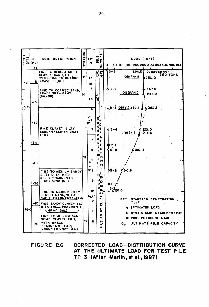
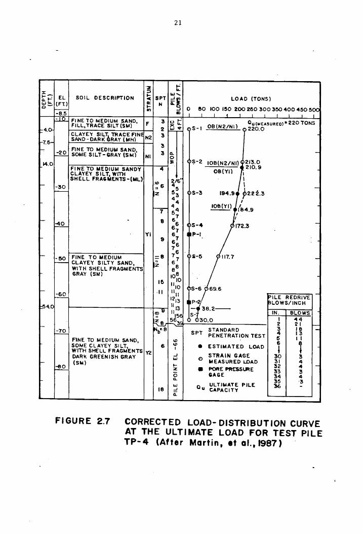
that was adjacent to the pile. Corrections of the load

distribution curves at the limit load attributed to

possible stresses imposed by the weight of the load frame

are shown in Figures 2.6 and 2.7 for piles TP-3 and TP-4

respectively_ Since the effects of possible eccentricity

could not be measured during testing, corrections for this

factor were not applied.

Based on the corrected load distribution curve

for pile TP-3, the unit shaft resistance was found to vary

from 0.7 to 1.4 tsf in the upper stratum of the Yorktown

~ x .... ;: EL Q..I.I..

501 L DESCRIPTION .....

oe SPT ~ _ (FT.) ~

7.1 FINE TO MEDIUM SilTY CLAYEY SAND, FILL, .

I- WITH FINE TO COARSE ?O- . 0 GRAVEL ~ (SC)

~ N .,

F 14

15

4 FINE TO COARSE SAND, TRACE SILT:":.GRAY '. HI (SM- SP)

.... 1..;.20

FINE CLAYEY SILTY -I--SAND- GREENISH GRAY (SM)

I-

130

I--

Y.I I-

-40 r---

- FINE TO MEDIUM SANOY SILTY CLAY, WITH SHELL FRAGMEN TS -

I- LIGHT GRAY (ell -50 t--

r- FINE TO MEDIUM SILTy CLAYEY SAND, WITH _St1.Eu... F RAGM ENT S -15M

12 -so FINE SANOY CLAYEY SU t-- WITH SHELL FRAGMENTS

1--69.0 ~ GRAY' (NL) .r-t-- 8

FINE TO MEOI UM SAND, SOME CLAYEY SilT,

_ WITH SHELL ~ FRAGMENTS-DARK

GREENISH GRAY (SM)

Y2 9

20

LOAD (TONS)

o &0 100 I~O 200 2.50 300 3!50 400 4&0 &OC -.l I I t I I It'

$- I 250.6 Qu (WEASURED) :: .

c~S-4

I.~;-l c~ S-S

OB(F/Nt) .2&0.0 260 TONS _

IOB(F/NI)

lOB (YI)

I, 247.5

j 245.9 I t , , . . 9 2,82.5 I , , , , ,

, 221.0 214.9

·169.5

-

--

-

.

:..

..

05-8 90.6 -

aPT STANDARD PENETRATION TEST •

• ESTIMATED LOAD

CD STRAiN UaE MEASURED LOA,[J

• PORE PRESSURE .AGE

Qu ULTIMATE PILE CAPACITY -

FIGURE 2.6 CORRECTED LOAD- DISTRIBUTION CURVE AT THE ULTIMATE LOAD FOR TEST PILE TP-3 (After Martin. at a1.,1987)

X t--:-o..t-wLl.. 0-

:4.0-

.... 7.6-r-

,...14.0

--.

I-

-!-

-

-t:;54.0

r-

r-

"'"

21

'2 ..,: "'-:l "" ..... ....

LOAD (TONS) EL SOIL DESCRIPTION til SPT

~~ (FT.) It: H .... 0 50 100 I~O 200 260 300 3!50 400 0450500 t--- In

-8.5 I:) I I J i -.1. .1 .J. .1 .l I I

~ FI NE TO MEDIUM SAND, 3 ..,: CU (tw1EASUREO)· 220 TONS F "'Lt.. Fill, TRACE SILT (5M) )(..,.

(, S-I OB{N2/Nll 9 220.0 '2. ..!!:!..-CLAYEY SllTe TRACE FINE 3 -SAND-DARK RAY (MHl N2

3 ,-20

FINE TO "'EOIUM SAND. 3 Q.. -SOME SILT-GRAY (SM) NI 0

~ 4'l?-2 IOB(N2/NI) I 213.0 FI NE TO MEDIUM SANOY 4J OB(VI} ,

,210.9 -CLAYEY SilT, WITH I SHEll FRAGMENTS-(Ul) 216'

, .CD 6

45 ,

--30 n

~222.3 r-- :z 53 1';>5-3 194.9 44 I

4.q 108(YI) ~ 1'84.9 --r 57 I

I . 8 66 -,-40

6 7 C·~S-4 172.3

VI 67

•• P-I. 9 6 6

. . 76

-&0 FINE TO MEDIUM =8 77 1'~$-5 . 117.7 -CLAYEY SILTY SAND. I! 6 r--

2 ee WITH SHELL F~AGMENTS GRAY (SM) e .

tOlO If> 1110 C $-6 69.S

-60 ·11 "11 PilE REDRIVE -t--- 1;'>'3 IIP- ~lOWS/INCH "'3 ' co 1:J II >E

38.2--IN. BLOWS .

S-II 5l~c ~:> • 30.0 I 414 ~ ~ 2 21 r--INbee STANDARD 3 18 --70 SPT 4 13 - PENETRATION TEST 5 I I FINE TO MEDIUM SAND, CD 6 1 SOME CLAYEY SILT, 6 CD • ESTIMATED LOAD , -I WITH SHELL FRAGMENTS Y2 J STRAIN GAGE 30 3 DARk GREENISH GRAY w E)

MEASURED LOAD 31 4 (SM) ~ 32 4 -;eo z • PORE PRESSlME 33 3 0 GAGE 34 4 0.. 35 '3

Q UlTl-..ATE PilE w 36 -18 ::: U CAPACITY n.

FIGURE 2.7 CORRECTED LOAD- DISTRIBUTION CURVE AT THE ULTIMATE LOAD FOR TEST PILE TP- 4 (After Martin t et al .• 1987)

22

formation. The load distribution curve for pile TP-4 also

produced similar results. Unit shaft resistance varied

between 0.6 to 1.2 tsf within Stratum Cl. These variations

are attributed to changes in relative densities throughout

this stratum.

Unlike pile TP-3 which was

within Stratum Cl, the last five feet

embedded totally

of pile TP-4 was

embedded within the more granular soil of Stratum C2. The

load-distribution curve disclosed a unit shaft resistance

of 0.5 tsf for Stratum C2.

The unit point resistance as reflected by the

load-distribution curves for

pile

piles

tip

TP-3 and TP-4 were

slightly different. The

Stratum C2 produced a unit

of TP-4

point resistance

supported by

of 28.7 tsf

whereas the pile tip of TP-3 which was supported by the

finer grain soils of Stratum Cl produced a lower unit point

resistance of 20.6 tsf.

Although the point resistance for pile TP-4 was

greater than pile TP-3 t the ultimate load capacity was

slightly less as determined from the load-settlement data.

This was most likely due to variation in unit skin

resistance throughout Stratum Cl.

Chapter 3

SOIL SAMPLING AND IN-SITU TESTING

3.0 Introduction

One of the requirements in the determination of

pile capacity and behavior is the analysis of subsurface

conditions, index properties and strength- deformation

characteristics of the soil medium in which the pile is

embedded. In the preceding chapter, results of subsurface

investigations and pile load tests were presented.

However, these data were insufficient to perform the finite

element method of analysis undertaken in this study.

Therefore, it was necessary to conduct additional soil

investigations.

Soil sampling was performed within a single bore

hole using both "disturbed" and "undisturbed" methods;

specifically, split spoon

Standard Penetration Tests

and Shelby tube samplers.

and Menard Pressuremeter Tests

were also performed. The purposes of these sampling

procedures and tests were twofold: to obtain representative

samples of the soil medium in which the piles were embedded

for use in soil laboratory tests and secondly, to determine

the in-situ strength and deformation characteristics of the

soil medium.

The soil sampling and in-situ tests were limited

23

24

to a single test boring performed just prior to

installation of production piles at the site on April 24,

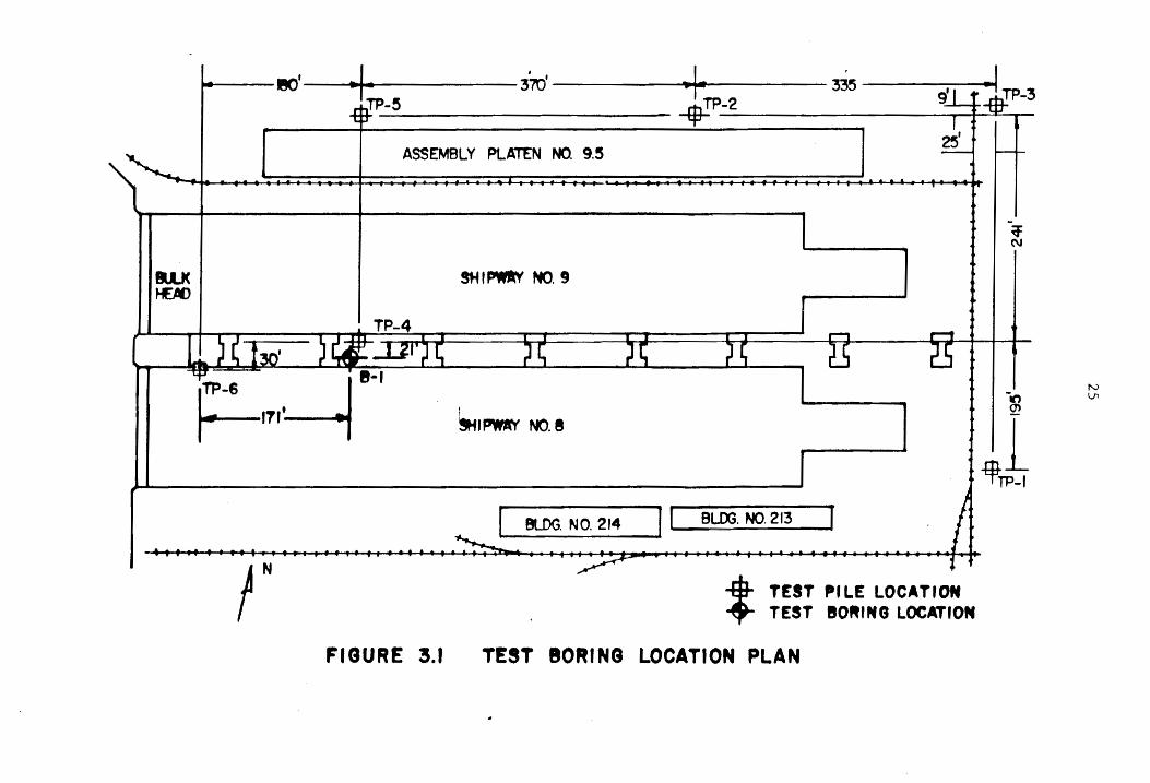
1984. The location selected was approximately 21 feet

south of pile TP-4 as shown on Figure 3.1. The areas near

test piles TP-3 and TP-5 were not accessable at the time of

this study.

The soil boring was drilled by Foundation Testing

Services of Bethesda, Maryland. The borehole was drilled

by a 3.5 inch hollow stem auger attached to a truck mounted

drill rig, Model CME-45B. The boring extended from the

ground surface to a depth of 75.0 feet. Since the load

bearing capacity of piles is attributed primarily to Strata

Cl and C2 soils within the Yorktown formation, sampling was

limited to these soils. In-situ tests incorporated within

the test boring program included Standard Penetration Tests

and Menard pressuremeter tests.

3.1 Soil Sampling and Standard Penetration Tests

The boring operation included sampling subsurface

soils of the Yorktown formation from a depth of 14.5 to

75.0 feet below the ground surface. Both split spoon and

Shelby tube samplers were used at intervals of

approximately 10 feet. The subsurface soils of the Norfolk

formation were not sampled since they were found to have

little impact on pile behavior for reasons already stated.

flU( f£I()

.. 8)' .1 & 370' .+ 335 <I

1P-~ ..J1:L TP-2 'f' --------------------~T~~~-

ASSEMBLY PLATEN NO. 9.5

1~-6 . 18

-1

r-111~

IN FIGURE 3.1

9H 'PWII:f NO. 9

i ~'PWAV NO.8

[-~elDG. NO. 214 J ( BUX;. NO. 213 ]

• TEST PILE LOCATION ... TEST 80RING LOCATION

TEST BORING LOCATION PLAN

~ N

-~

1 tV-TP-'

N V'1

26

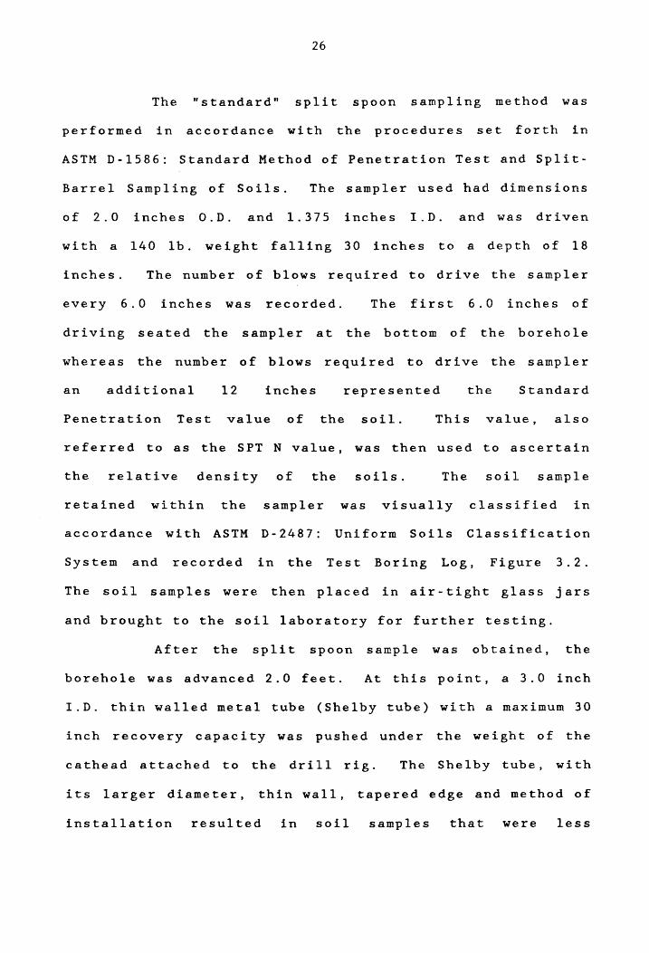
The "standard" split spoon sampling method was

performed in accordance with the procedures set forth in

ASTM D-1586: Standard Method of Penetration Test and Split­

Barrel Sampling of Soils. The sampler used had dimensions

of 2.0 inches O.D. and 1.375 inches I.D. and was driven

with a 140 lb. weight falling 30 inches to a depth of 18

inches. The number of blows required to drive the sampler

every 6.0 inches was recorded. The firs t 6.0 inches of

driving seated the sampler at the bottom of the borehole

whereas the number of blows required to drive the sampler

an additional 12 inches represented the Standard

Penetration Test value of the soil. This value, also

referred to as the SPT N value, was then used to ascertain

the relative density

retained within the

of the soils. The soil sample

sampler

accordance with ASTM D-2487:

was visually

Uniform Soils

classified in

Classification

System and recorded in the Test Boring Log, Figure 3.2.

The soil samples were then placed in air-tight glass jars

and brought to the soil laboratory for further testing.

After the spli t spoon sample was obtained, the

borehole was advanced 2.0 feet. At this point, a 3.0 inch

1.0. thin walled metal tube (Shelby tube) with a maximum 30

inch recovery capacity was pushed under the weight of the

cathead attached to the drill rig. The Shelby tube, with

its larger diameter, thin wall, tapered edge and method of

installation resulted in soil samples that were less

,== I _lJ

27

rlNE TO I'1(OllJM SltH SANO (S111 ~Il!l SHell fHACiI'I[tIlS. "'1$1 • GUY

flN( 10 I'I[Ol\J'1 SANOr a..un Sill (til I.II1H snEll fUCft{HT$. ftOlST • GNU

Itl[Ll

rllC( 101'1(01"" SANO. 1011( IH' (srI!, IoIITIl Stlnl 'IAGI'I(IfTS. fIOU' • nANa: c;n[[H

SPU T sre'0I1 SAI1PL(1I lOCAJJON

I. $Il( L IT 1 ul£ SA/\PL (II l OCA 11 ON

FIGURE 3.2 TEST BORING r.a:;

".". Hlil NO. h I)' • 17'

".rI. IUT 110. 2; 2'.)' - 27'

P.". nSI 110. 3: JS' • 37'

',rI. TEST NQ.1.f; 1f5' • 'l7'

P ,rI. Icsr NU. 5: ~S' • 51'

P.rI;.,1£U 110. 6. ;:at' • sg'

".". J(ST 1IfIO. 1. £6' • 67'

tl'l(..a .. N[ IUl'hllllCol "PI, HST MI. II 6t!' • 1!J' (CONfllOl IU:t tu.lfUNClJl,lHl ',PI, JUT 110. 91 n' . )\(' (",,..,,IIt( IVI"IUlt(D I

28

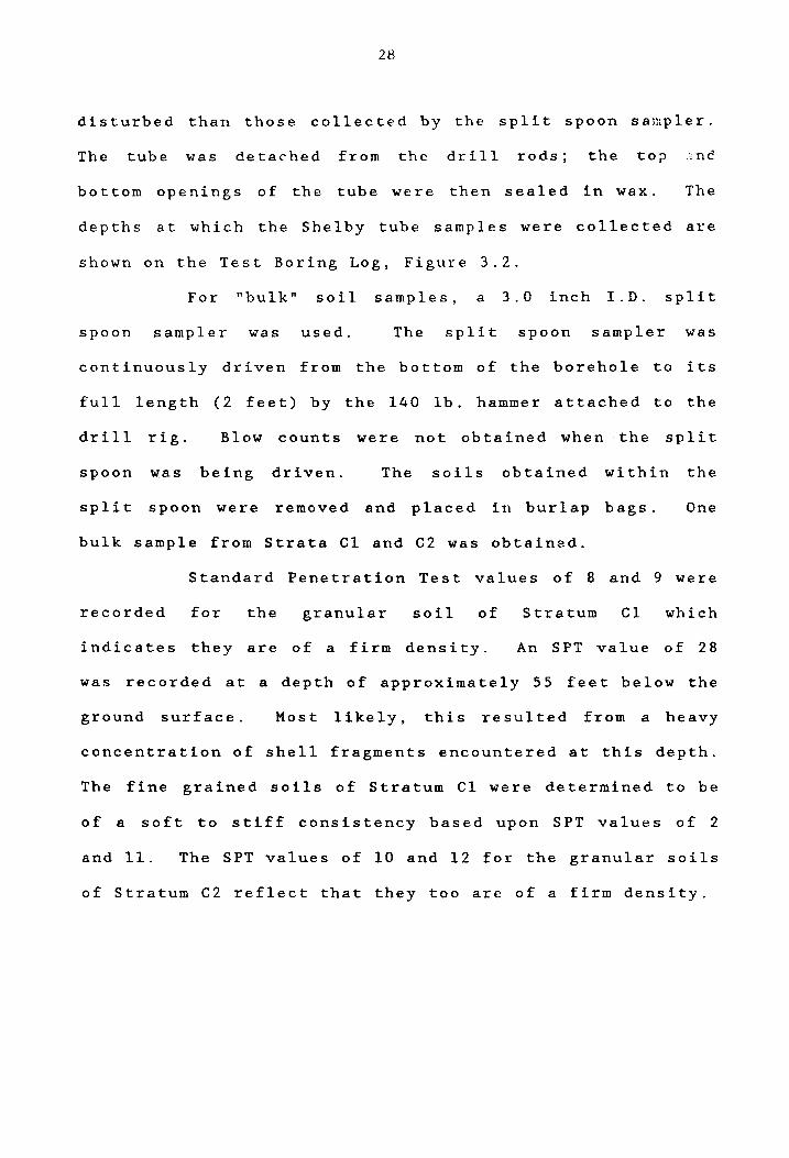
disturbed than those collected by the split spoon

The tube was detached from the drill rods; the

sampler.

top nd

bottom openings of the tube were then sealed in wax. The

depths at which the Shelby tube samples were collected are

shown on the Test Boring Log, Figure 3.2.

For "bulk" soil samples. a 3.0 inch I.D. split

spoon sampler was used. The split spoon sampler was

continuously driven from the bottom of the borehole to its

full length (2 feet) by the 140 lb. hammer attached to the

drill rig. Blow counts were not obtained when the split

spoon was being driven. The soils obtained within the

spli t spoon were removed and placed in burlap bags. One

bulk sample from Strata Cl and C2 was obtained.

Standard Penetration Test values of 8 and 9 were

recorded for the granular soil of Stratum CI which

indicates they are of a firm density. An SFT value of 28

was recorded at a depth of approximately 55 feet below the

ground surface. Most likely, this resulted from a heavy

concentration of shell fragments encountered at this depth.

The fine grained soils of Stratum Cl were determined to be

of a soft to stiff consistency based upon SPT values of 2

and 11. The SPT values of 10 and 12 for the granular soils

of Stratum C2 reflect that they too are of a firm density.

29

3.2 Menard Pressuremeter Tests

The pressuremeter test was first conceived by

F. Kogler of Germany in 1933 and subsequently developed by

M. Louis Menard in 1956 as a means of determining the in­

situ strength-deformation characteristics of soils. The

test involves the expansion of a cylindrical probe beneath

the ground surface in order to measure the relationship

between pressure and the resultant deformation of the soil.

Soil properties are then calculated from the test data

utilizing elastic-plastic or rheological theory.

3.2.1 Pressuremeter Test Apparatus

There are several types of pressuremeters,

however, the probe, control unit and tubing are common to

all as illustrated in Figure

make-up of each of these

3 . 3 . Details concerning the

components can be found in

reference (1). In this study, Menard Pressuremeter Model

No. GC was used. This unit is best suited for soils of a

soft to stiff consistency.

The probe, which is inserted within the borehole,

applies a radial pressure along the walls of the borehole

and simultaneously measures the increase in volume of the

hole. At both ends of the probe are guard cells inflated

by compressed bottled gas to the same pressure as the

Control Unit

30

guard cell

Probe % measuring cell /

FI GU RE 3.3

%~ guard cell

~ PRINCIPLE COMPONENTS OF THE

MENARD PRESSUREMETER

31

measuring cell. This insures that deformation is radial.

An outer shea th of heavy rubber f neoprene or rubber wi th

steel straps is

measuring cell

attached to the

from puncture.

probe

In

investigation performed for this study,

to protect the

the subsurface

a steel strap

sheath was used due to the high concentration of shell

fragments.

The control unit. consisting of a graduated water

cylinder (volumeter) and regulator, controls and monitors

expansion of the probe through tubing that conveys the

water and gas from the control unit to the probe.

Equal increments of pressure are applied to the

probe and the stress levels are held constant for a fixed

length of time, usually one minute. Volume changes are

recorded at intervals of 15, 30 and 60 seconds for each

load application. The plot of the volumeter reading for

each pressure increment typically results in a curve of the

shape illustrated in Figure 3. 4a. This curve represents

readings derived from the control uni t. Certain

corrections for errors caused by the apparatus are required

in order to plot the actual pressure-volume response of the

soil. These corrections account for pressure gains and

losses introduced by the test apparatus itself. The degree

of correction required depends upon the particular type of

pressuremeter used.

The plot of the corrected volume and pressure

! en

f ~ 3

r---- ... --1--....---JA

I I

(""-~,..,.J I I ~_J P

L

I I I

~ I

I , I I

f I I

~ I I

i I I

~ • I

r-' I I

----"j

VOLUMETER READNG

TYPICAl UNCORRECTED PRESSUREMETER TEST' F£SULTS

(0 )

-' R ~PF

~

i i= ~

~

I t

'b

II I

1--- PRESSUREMETER CURVE

--- CREEP ClfM:

I

1-'(-Yo "F CHANGE IN VOUJME OF THE ~JTY

TYPICAL CORF£CTED PRESSEMETER TEST 'RESULTS

(b)

FIGURE 3.4 TYPICAl.. CCRRECTED A~ UNCORRECTED PREBORED PRESSUREMETER quRVES

W N

33

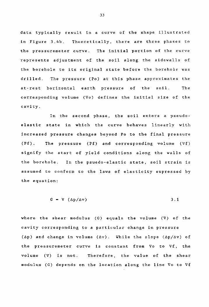
data typically result in a curve of the shape illustrated

in Figure 3. 4b. Theoretically, there are three phases to

the pressuremeter curve. The initial portion of the curve

represents adjustment of the soil along the sidewalls of

the borehole to its original state before the borehole was

drilled. The pressure (Po) at this phase approximates the

at-rest horizontal earth pressure of the soil. The

corresponding volume (Vo) defines the initial size of the

cavity.

In the second phase, the soil enters a pseudo­

elastic state in which the curve behaves linearly with

increased pressure changes beyond Po to the final pressure

(Pf). The pressure (Pf) and corresponding volume (Vf)

signify the start of yield conditions along the walls of

the borehole. In the psuedo-elastic state, soil strain is

assumed to conform to the laws of elasticity expressed by

the equation:

G - V (8p/Av) 3.1

where the shear modulus (G) equals the volume (V) of the

cavity corresponding to a particular change in pressure

(8p) and change in volume (8V). While the slope (8p/~V) of

the pressuremeter curve is constant from Vo to Vf, the

volume (V) is not. Therefore, the value of the shear

modulus (G) depends on the location along the line Vo to Vf

34

at which it is computed. Menard proposed that the volume

at the midpoint (Vm) between Vo and Vf be used to compute

the shear modulus.

follows:

The midpoint volume (Vm) is computed as

Vm - Vo + (Vo + Vf)/2

The Menard shear modulus

follows:

Gm - Vm(llp/6v)

(Gm)

3.2

is then calculated as

3.3

The value of Gm can also be determined directly from the

pressuremeter data by plotting IIp versus Ilv/V in which Gm

equals the slope of the curve between Vo to Vf.

For linear isotropic soils, the shear modulus may

be converted to Young's Modulus (E) as follows:

E - 2(1 + v)G 3.4

For the above relationship, Menard recommended that a

standard value of 0.33 be used for Poisson's ratio (v).

The resulting deformation modulus is referred to as the

Menard pressuremeter modulus

expressed by the formula:

(Epm) for a soil and is

35

Epm ... 2.66(Gm) 3.5

During the final phase, pressure increases above

the initial yield pressure (Pf) result in an increased rate

of volume change in the plastic deformation region and

eventually becomes asymptotic. The pressure along the

horizontal asymptote is referred to as the limit pressure

(PI) which is used to estimate the shear strength of the

soil. In general J the limi t pressure is taken as the

pressure required to double the initial volume of the

cavity.

Due to the limited number of data points

resulting from this process, it is difficult to accurately

interpret the values of Po and Pf from the pressuremeter

curve. In order to facilitate the determination of these

values, the change in volume that occurs between the 30

second and one minute reading versus the corresponding

pressure change is plotted as illustrated in Figure 3.4h.

This is referred to as the "creep curve" and the value of

Pf as the "creep pressure". The pressure (Po) and pressure

(Pf) correspond to the intersection of the two lines a-b

and b-c formed by the creep curve.

is rather

means of

In practice, interpretation of pressuremeter data

complex and therefore not usually suitable as a

direct measurement. The influence of soil

disturbance in forming the testhole and the inability to

36

determine drainage conditions during testing are among a

number of factors that can distort results (1). Thus, the

pressuremeter test is used mainly as a correlative tool to

determine the strength-deformation characteristics of soil

supported by other types of in-situ and soil laboratory

tests.

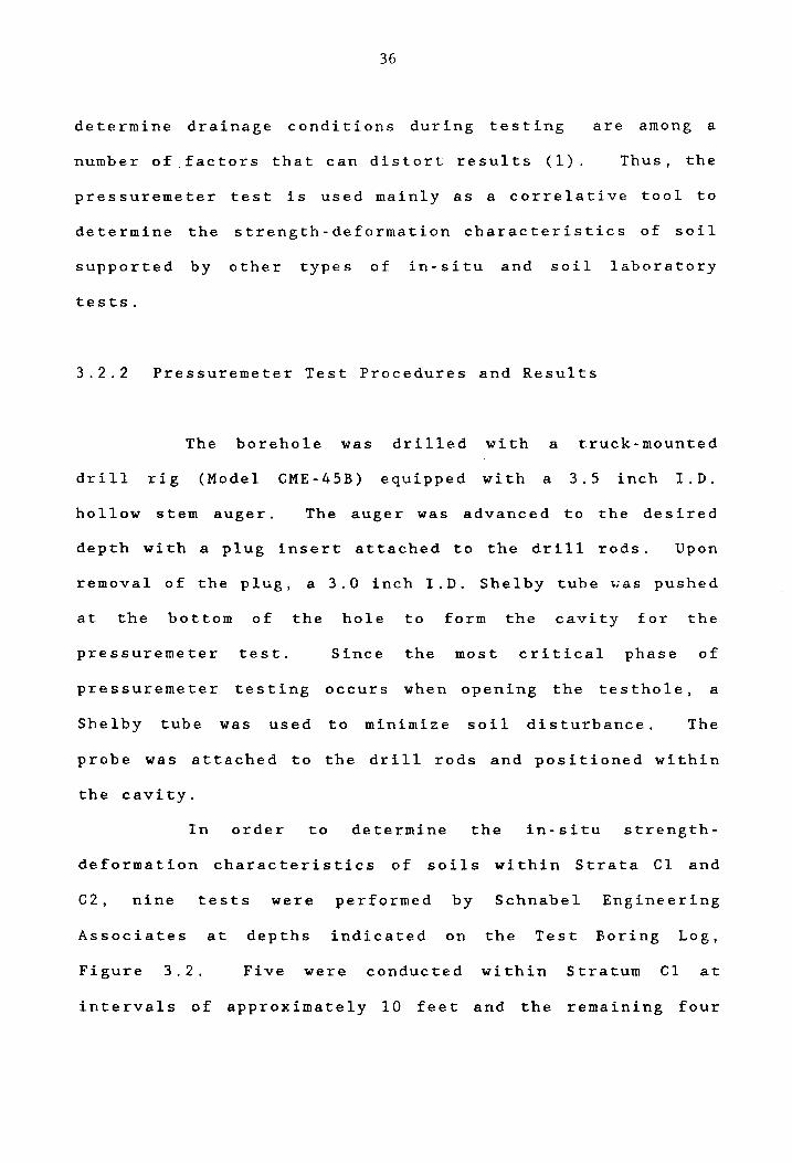
3.2.2 Pressuremeter Test Procedures and Results

The borehole was drilled with a truck-mounted

drill rig (Model CME-45B) equipped with a 3.5 inch I.D.

hollow stem auger. The auger was advanced to the desired

depth with a plug insert attached to the drill rods. Upon

removal of the plug, a 3.0 inch I.D. Shelby tube was pushed

at the bottom of the hole to form the cavity for the

pressuremeter test. Since the most critical phase of

pressuremeter testing occurs when opening the testhole, a

Shelby tube was used to minimize soil disturbance. The

probe was attached to the drill rods and positioned within

the cavity.

In order to determine the in-situ strength­

deformation characteristics of soils within Strata Cl and

C2, nine tests were performed by Schnabel Engineering

Associates at depths indicated on the Test Boring Log,

Figure 3.2. Five were conducted within Stratum Cl at

intervals of approximately 10 feet and the remaining four

37

within Stratum C2 at closure intervals less than five feet.

All nine tests were conducted within borehole B-1

drilled at the location shown in Figure 3.1. The elevation

and description of the soil type within the borehole are

also indicated in the Test Boring Log in Figure 3.2.

The pressuremeter and creep pressure curves from

six of the nine pressuremeter tests are included in

Appendix A. These data represent the corrected volume and

pressure readings after one minute and reflect the change

in volume which occurred between the 30 second and one

minute readings.

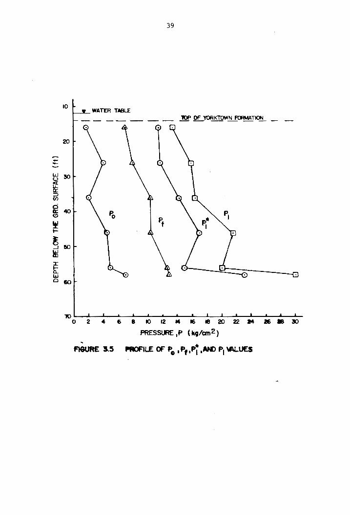
From the pressuremeter data, the values of Po,

Pf, PI, and Epm for pressuremeter tes ts PM-l through PM- 6

were determined. These are shown in Table 3.1. The change

in the values of Po, Pf and PI as a function of depth are

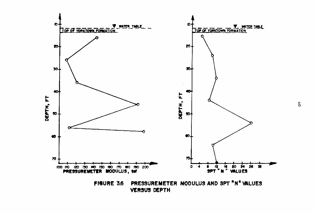
illustrated in Figure 3.5. Similarly, Figure 3.6 shows the

change in Epm and SPT values.

Insufficient data was collected from tests PM-7

through PM-9 because the rubber membrane of the measuring

cell ruptured; in addition, the pressure gauge

malfunctioned during test PM-S. These difficulties

resulted in pressuremeter data only for soils of the upper

Yorktown formation.

The values of Po, Pf and PI were found to

increase linearly

approximates the

with

total

depth. The

horizontal

value

stress

of

of

Po,

the

which

soil,

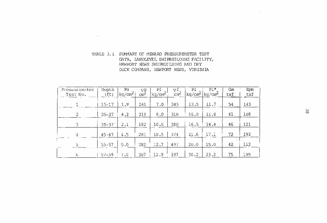
TABLE 3. 1 SU1MARY OF HENA.RD PRESSUREt1ETER TEST

Dl\TA, rANDLEVEL SHIFBUILDING FACILITY, NEWFDRT NEWS SHIPBUILDING AND DRY DOCK CO'1PANY, NB'lPORT NEW'S, VIRGINIA

Press ur sne ter D2 .h Po V o Pf kg/~ ~~ '1

kg/~rrf ·1*

Test No. (ft) kg/cm2 an2 kg/crrf

1 15-17 1.9 241 7.0 345 13.5 11.7

2 25-27 4.2 219 8.0 318 16.0 11.8

3 35-37' 2.1 182 10.5 380 16.5 14.4

4 45-47 4.5 281 10.5 374 21.6 17.1

5 55-57 5.0 282 12.7 497 20.0 15.0

6 57-59 7.0 _ 307 12.9 397 30.2 23.2 - -

tsf

54

41

46

72

42·

75

E[XrI

tsf

143

108

121

192

112

199

w co

39

10 WATER TABLE

20

--tot-

W !O ~ u:: ~ en d a:: 40 (!)

~ .....

~ !O liS :::I: ..... 0... UJ 0 10

~~~ __ ~~ __ ~~~~~~~ __ ~~ __ ~~ __ ~ __ ~-L-

o 2 4 6 8 10 12 M 16 18 20 22 1M 16. !O

PRESSlft:.p (k9/an2 )

FIGURE 5.5

_____ L WAtmT§.£..

---.,...--. II!nAMATtoN

....

i ~! ....

• ~ Z .... ~!O

0

•

10

100 110 .20 I!O MO 1!50 flO rm 110 190 200 ~!sU"!M!TIR MODULUS. ~

o 4 • Q ~ ~ MM. lIlT If ,.. w.lU ES

FIIURE 3.6 PRES9UREMETER MODULUS AND SPT ·N· 'ALUES VERSUS ~PTH

.t:--0

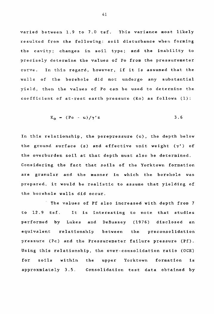
41

varied between 1.9 to 7.0 tsf. This variance most likely

resulted from the following: soil disturbance when forming

the cavity; changes in soil type; and the inability to

precisely determine the values of Po from the pressuremeter

curve. In this regard, however, if it is assumed that the

walls of the borehole did not undergo any substantial

yie ld, then the values of Po can be used to determine the

coefficient of at-rest earth pressure (Ko) as follows (1):

Ko = (Po - u)/~'z 3.6

In this relationship, the porepressure (u), the depth below

the ground surface (z) and effective unit weight (~') of

the overburden soil at that depth must also be determined.

Considering the fact that soils of the Yorktown formation

are granular and the manner in which the borehole was

prepared, it would be realistic to assume that yielding of

the borehole walls did occur .

. The values of Pf also increased with depth from 7

to 12.9 tsf. It is interesting to note that studies

performed by Lukes and DeBussey (1976) disclosed an

equivalent relationship between the preconsolidation

pressure (Pc) and the Pressuremeter failure pressure (Pf).

Using this relationship, the over-consolidation ratio (OCR)

for soils within the upper Yorktown formation is

approxmiately 3.5. Consolidation test data obtained by

42

Schnabel Engineering for samples within this stratum

yielded an OCR value of 3.2. Thus, the indicated values of

Pf correlate well with values of Pc.

With regard to using the value of PI from

pressumeter data to determine the shear strength of soils,

studies have revealed that only the undrained shear

strength of cohesive soils can be determined with any

degree of accuracy (9). In the relationship developed by

Menard, the undrained shear strength (Su) is expressed as

follows:

Su - (Pl-Po)/2K 3.7

where K is a variable coefficient that reflects soil type,

relative density and soil structure. Gibson and Anderson

(9) suggested a similar relationship for determining the

undrained shear strength using the cohesive strength (c) of

the soil and Poisson's ratio (v) as follows:

Su -PI-Po 3.8

1 + In{Epm/[2c(l+v)]}

In both equations, the value of Su is determined in part by

the difference in the value of PI and Po. This is

referred to as the net limiting pressure (Pl*):

PI* - PI-Po 3.9

43

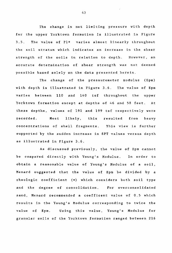
The change in net limiting pressure with depth

for the upper Yorktown formation is illustrated in Figure

3 . 5 . The value of Pl* varies almost linearly throughout

the soil stratum which indicates an increase in the shear

strength of the soils in relation to depth. However, an

accurate determination of shear strength was not deemed

possible based solely on the data presented herein.

The change of the pressuremeter modulus (Epm)

with depth is illustrated in Figure 3.6. The value of Epm

varies between 110 and 140 tsf throughout the upper

Yorktown formation except at depths of 46 and 58 feet. At

these depths, values of 191 and 199 tsf respectively were

recorded. Most likely, this resulted from heavy

concentrations of shell fragments. This view is further

supported by the sudden increase in SPT values versus depth

as illustrated in Figure 3.6.

As discussed previously, the value of Epm cannot

be compared directly wi th Young's Modulus. In order to

obtain a reasonable value of Young's Modulus of a soil,

Menard suggested that the value of Epm be divided by a

rheologic coefficient (0::) which considers both soil type

and the degree of consolidation. For overconsolidated

sand, Menard recommended a coefficent value of 0.5 which

results in the Young's Modulus corresponding to twice the

value of Epm. Using this value, Young's Modulus for

granular soils of the Yorktown formation ranged between 216

44

and 288 tsf.

In brief, the pressuremeter data collected in

conjunction with this study suggests:

1. The soil throughout the Yorktown formation is

preconsolidated and has an OCR value of 3.5 based on the

values of Pf.

2. Shear strength of the soil generally increases

linearly with depth. This was evidenced by the increase in

net limit pressure (Pl*) found throughout the Yorktown

formation.

3. Insufficient data was available to allow for a

reasonable determination of the actual strength of the

soil.

4. Young's Modulus (E) values range from 216 to

288 tsf for the granular soils of the upper Yorktown

formation.

5. Further pressuremeter testing within this soil

formation must be conducted if a better correlation of

pressuremeter data and soil properties is to be made.

Chapter 4

SOIL LABORATORY TESTS

4.0 General

The answer to a problem in Geotechnical

engineering is normally obtained by first determining the

properties of the soil in question and then employing these

properties in predictive solutions. Often, soil properties

can be effectively determined by soil laboratory testing.

Soil sampling and in-situ tests were performed in

order to identify the soil type and relative density of the

soil medium being investigated to include its in-situ

strength-deformation characteristics. For further

evaluation of the properties of the various soil types,

soil laboratory tests were conducted. These were performed

on the six Shelby tube samples obtained from the test

boring for the following purposes:

determination of key strength

soil identification;

characteristics; and

establishment of hyperbolic soil parameters.

The strength properties of the soil medium are an

important part in evaluating pile behavior. In this

connection, Menard pressuremeter tests were conducted to

obtain the in-situ strength-deformation characteristics of

the soil.

adequate

However, the data obtained was not deemed

to accurately determine the strength

45

46

characteristics. For this reason, triaxial tests were

performed to better evaluate the strength characteristics

of the soil medium. Along the soil-pile interface, it was

not possible to determine the strength properties by

conventional triaxial test methods. For this case, a soil-

concrete interface test program was developed and is

discussed later in this report.

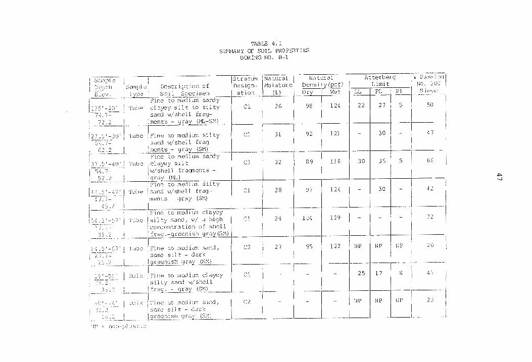
4.1 Basic Soil Properties and Classification

The moisture content, natural density, Atterberg

Limits, and grain size distribution were determined for

each of the six Shelby tube samples obtained from the test

boring. The term natural density refers to the soil

dens i ty wi thin the Shelby tube which may vary from the

actual in-situ density due to disturbance of the soil

during sampling and transport. The classifications

presented herein are based upon ASTM D-2487: Classification

of Soils For Engineering Purposes. The laboratory results

and description of the samples tested are summarized in

Table 4.1.

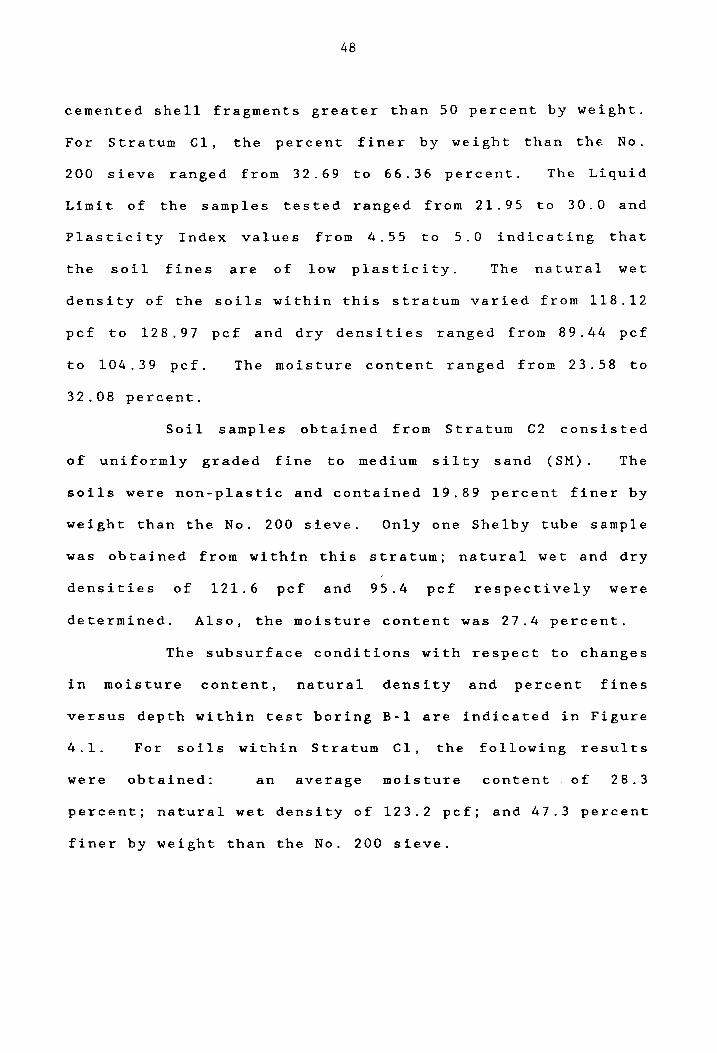
In general, the samples obtained from Stratum Cl

were found to consist of fine to medium sandy clayey silt

(ML) and silty sand (SM) with varying amounts of shell

fragments. At a depth of approximately 55 ft. below the

ground surface, the soils contained high concentrations of

L7S' 20' -----.----

.2

5 i 1 t to sil ty sard .... '/shell frag­ments

27 .5' - 30 ' Tube' Fine to lTI(-:lJ iU11 sD ty sarD \v/shell

TABLE 4.1 SU'-ll1ARY <F SOIL PROPERTIES

BORHJG NO. 8-1

31

C1 8 97

Ci_ 4 101

C2 -;

Cl

C2

30

o 35

24 30

122

5

l~P

32

41

2

~ '-..l

48

cemented shell fragments greater than 50 percent by weight.

For Stratum C1, the percent finer by weight than thE No.

200 sieve ranged from 32.69 to 66.36 percent. The Liquid

Limit of the samples tested ranged from 21.95 to 30.0 and

Plasticity Index values from 4.55 to 5.0 indicating that

the soil fines are of low plasticity. The natural wet

density of the soils within this stratum varied from 118.12

pcf to 128.97 pcf and dry densities ranged from 89.44 pcf

to 104.39 pcf. The moisture content ranged from 23.58 to

32.08 percent.

Soil samples obtained from Stratum C2 consisted

of uniformly graded fine to medium sil ty sand (SM). The

soils were non-plastic and contained 19.89 percent finer by

weight than the No. 200 sieve. Only one Shelby tube sample

was obtained from within this stratum; natural wet and dry

densities of 121.6 pcf and 95.4 pcf respectively were

determined. Also, the moisture content was 27.4 percent.

The subsurface conditions with respect to changes

in moisture content, natural density and percent fines

versus depth within test boring B-1 are indicated in Figure

4.1. For soils within Stratum Cl, the following results

were obtained: an average moisture content of 28.3

percent; natural wet density of 123.2 pcf; and 47.3 percent

finer by weight than the No. 200 sieve.

z • o t­~

~ ~

t :)

il I • 1 0 I~~ I1lt~

~I~~ CI

lir A

> /1

II I I I I

~~ I"

',I Il~A

I \ I\. I 'lr,A I " I I / I /

~/ I

to 100 110

il z -I B '" I a:: .... ;,Ei ;1

o o

,.. ~ N 1 • "'.1 II: ~ Ilr~ !I :l~ c,

I '/-1 z - ~ '" 0 ..... ·1 a:t-.. !t'~

~I§~ c 1

I

10 H 30 55- 10 30 40 10 10

NATURAL DENSITY. MOISTURE CXWTENT," °4PASSING NO.200 91EVE

• SHELL FRAGMENTS I2J SHELBY TUBE SAMPLE

FIGURE 4.1 SUBSURFACE PROFILE OF SOIL PROPERTIES

~ \.0

50

4.2 Triaxial Testing of Soil Samples

The strength characteristics of a particular soil

type is dependent upon the state of the soil before and

during shearing to include drainage conditions and

consolidation of the soils. Along the soil-pile interface

and at the pile tip, shearing of the soils were assumed to

behave under consolidated-drained (CD) conditions. The

soil medium away from the pile perimeter beyond the soil-

pile interface was assumed to behave under the

consolidated-undrained (CU) condition. Therefore, a CU

triaxial test was performed on a Shelby tube sample

representing soils of the upper Yorktown formation (Stratum

Cl) . Below the pile tip, the soil medium was considered to

represent that of Stratum C2 in the case of the model pile.

Hence, a representive Shelby tube sample was tested under

consolidated-drained (CD) conditions.

Duncan et al. (1980) outlined procedures for

determining stress-strain and volume change parameters that

represent the non-linear and stress dependent stress-strain

and volume change behavior of soil. These parameters are

based upon hyperbolic stress-strain relationships which

provide a framework that encompasses the most important

characteristics of stress-strain behavior: non-linearity;

stress - dependency; and inelastici ty. Nine parameters are

employed in the hyperbolic stress-strain relationship used

51

to determine soil behavior (Table 4.2).

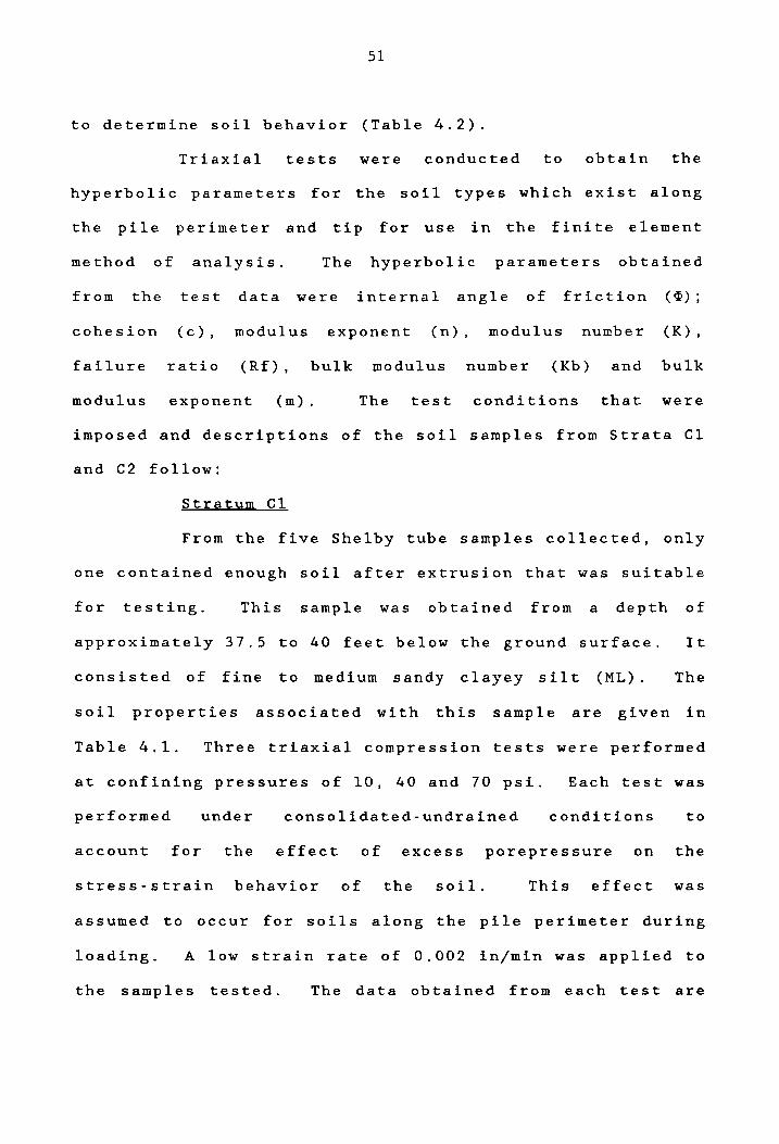
Triaxial tests were conducted to obtain the

hyperbolic parameters for the soil types which exist along

the pile perimeter and tip for use in the finite element

method of analysis. The hyperbolic parameters obtained

from the test data were internal angle of friction (~);

cohesion (c), modulus exponent (n), modulus number (K),

failure ratio (Rf), bulk modulus number (Kb) and bulk

modulus exponent (m). The test conditions that were

imposed and descriptions of the soil samples from Strata Cl

and C2 follow:

Stratum Cl

From the five Shelby tube samples collected, only

one contained enough soil after extrusion that was suitable

for testing. This sample was obtained from a depth of

approximately 37.5 to 40 feet below the ground surface. It

consisted of fine to medium sandy clayey silt (ML). The

soil properties associated with this sample are given in

Table 4.1. Three triaxial compression tests were performed

at confining pressures of 10, 40 and 70 psi. Each test was

performed under consolidated-undrained conditions to

account for the effect of excess porepressure on the

stress-strain behavior of the soil. This effect was

assumed to occur for soils along the pile perimeter during

loading. A low strain rate of 0.002 in/min was applied to

the samples tested. The data obtained from each test are

Parameter

K, Kur

n

c

~, 0$

Rf

~

m

TABLE 4.2 SUMMARY OF THE HYPERBOLIC PARAMETERS (After DUNCAN, et 01.,'980)

Name Function

Modulus number

Modulus exponent Relate Ei and E to 03 ' ur

Cohesion intercept Relate (01-03)f to 03

Friction angle parameters

Failure ratio Relates (Ol-0 3)ult to (01-03)f

Bulk modulus number Value of SIp at 03 ~ P a a

Change in B/Pa for ten-fold Bulk modulus exponent

increase in 03

Ln N

53

shown in Appendix B.

Stratum C2

One Shelby tube sample was collected from this

stratum at a depth between 64.5 to 67 ft. below the ground

surface. The soil consisted of fine to medium sand with

s i 1 t (SM). Three triaxial compression tests were also

performed on this sample at confining pressures of 10, 40

and 70 psi. The test sample represented soils at the pile

tip for which drainage was assumed to have occured during

loading. Thus, each sample was tested under consolidated-

drained conditions. In order to facilitate drainage, a low

strain rate of 0.005 in/min was applied. The data obtained

from each of the samples tested are included in Appendix C.

The confining pressures imposed were selected

based upon horizontal earth pressures determined from the

Menard pressuremeter tests which indicated a range between

29 psi to 99 psi.

The procedures used to determine the desired

hyperbolic parameters were those established by Duncan et

al. (1980). From the triaxial test data, stress versus

strain curves corresponding to a particular confining

pre s sure (a3) were deve loped as shown in Figure 4.2 in

which the ultimate deviatoric stress (al-a3) for each value

of a3 was determined. In addi tion, the ini tial Young's

Modulus (Ei) which varies with values of u3 was determined

from the initial slope of the stress-strain curve. Using

54

'.

REAL £ ("i -CT 3) = -----E--

-' + ----=~-Ei (q -0-3 )ult

E

TRANSFORMED

____ G_ = _1_ + C

(OJ -0'"3) E ~ (Oi -0-3)u It

E

FIG. 4.2 HYPERBOLI C REPRESENTATION OF A STRESS-STRAIN CURVE (After Duncan, at al., 1980)

55

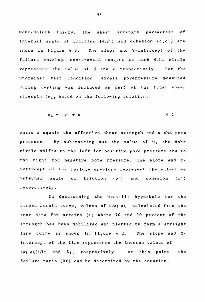
Mohr-Columb theory, the shear strength parameters of

internal

shown in

failure

angle of

Figure

envelope

friction (~,~') and

4.3. The s lope and

constructed tangent

cohesion (c,c') are

Y-intercept of the

to each Mohr circle

represents the value of 4> and c respectively. For the

undrained test condition, excess porepressure measured

during testing was included as part of the total shear

strength (at) based on the following relation:

at - 0' + u 4.1

where 0 equals

pressure. By

the effective shear strength and u the pore

subtracting out the value of u, the Mohr

circle shifts to the left for positive pore pressure and to

the right for negative pore pressure. The slope and Y­

intercept of the failure envelope represent the effective

internal angle of friction (~' ) and cohesion (c' )

respectively.

In determining the best-fit hyperbola for the

stress-strain curve, values of E/ol-03 calculated from the

test data for strains (E) where 70 and 90 percent of the

strength has been mobilized and plotted to form a straight

line curve as shown in Figure 4.2. The s lope and Y-

intercept of the line represents the inverse values of

(al-03)ult and Ei' respectively. At this point, the

failure ratio (Rf) can be determined by the equation:

1:'

2 C COS 4> + 20"3 SIN 4> (0; -(3) ': I

If· I-SIN</>

CIt .. (OJ-0"3)f= Rf {Oj-CT3 )ult

a-

FIGURE 4.3 VARIATION OF STRENGTH WITH CONFINING PRESSURE (After Duncan t at at. 1980)

\J1 ~

(01-03)ult (°1-°3) f

57

4.2

where (01-03)f represents the deviatoric stress at failure

w hie his a 1 way s 1 e sst han ( 01-03 ) u 1 t . The variation of Ei

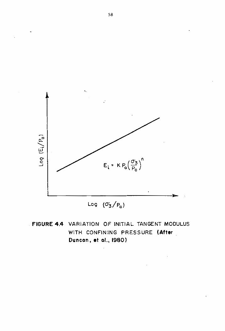
with 3 is represented by the following equation:

4.3

where Pa is atmospheric pressure. For determining values

of K and n, values of (Ei/Pa) versus (03/Pa) were plotted

on log-log scale as shown in Figure 4.4. The slope of the

line represents the value of n and the Y-intercept the

value of K.

The relationship between changes in Young's

Modulus with stress is represented by the instantaneous

slope of the stress-strain curve, referred to as the

tangent modulus (E t ). Duncan et al. (1980) formulated that

the appropriate value of the tangent modulus can be

calculated for any stress condition (03 and 01-03) by the

following expression:

KPa(p!J 4.4

In order to account for the non-linear volume change for

. -w

0" o ..J

58

....

, FIGURE 4.4 VARIATiON OF INITIAL TANGENT MODULUS

WITH CONFIN ING PRESSURE (After

Duncan t et 01., 1980)

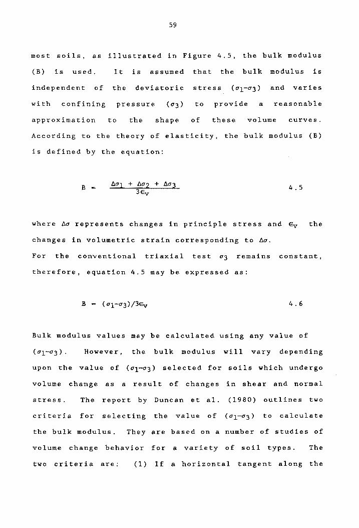
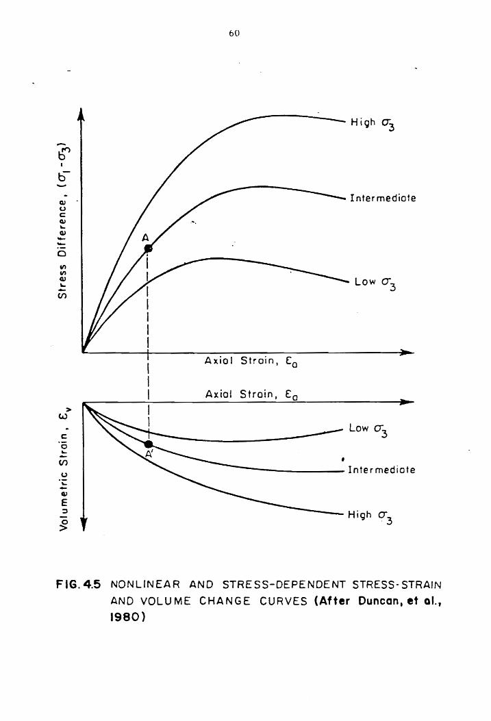
59

most soils, as illustrated in Figure 4.5, the bulk modulus

(B) is used. It is assumed that the bulk modulus is

independent of the deviatoric stress (0'1-0'3) and varies

with confining pressure to provide a reasonable

approximation to the shape of these volume curves.

According to the theory of elasticity, the bulk modulus (B)

is defined by the equation:

B -fiUl + fiu2 + fiu3

3Ev 4.5

where ~u represents changes in principle stress and Ev the

changes in volumetric strain corresponding to ~u.

For the conventional triaxial test 0'3 remains constant,

therefore, equation 4.5 may be expressed as:

Bulk modulus values may be calculated using any value of

However, the bulk modulus will vary depending

upon the value of (0'1-0'3) selected for soils which undergo

volume change as a result of changes in shear and normal

stress. The report by Duncan et al. (1980) outlines two

criteria for selecting the value of (0'1-0'3) to calculate

the bulk modulus. They are based on a number of studies of

volume change behavior for a variety of soil types. The

two criteria are: (1) If a horizontal tangent along the

-~ I

b

OJ u c: OJ ~

Q.I --0

VI VI OJ "--en

,. w

c: o ~

(f)

u ~ -CIJ

E ::J

~

60

H i<jh 0"3

Intermediate

Low 0-3

Axial Strain, (0

Axial Strain,

Low 0'"3

• ---------- Intermediate

FIG.4.5 NONLINEAR AND STRESS-DEPENDENT STRESS-STRAIN

AND VOLUME CHANGE CURVES (After Duncan. et 01., 1980)

61

volume change curve is not reached at the point at which 70

percent of the stress has been mobilized, then

corresponding Ev values at the 70% stress level should be

used and (2) If the horizontal tangent is reached at 70% of

strength mobilization along the volume curve, then use the

values 0 f (°1-°3) and corresponding Ev value a t the po int

on the volume curve where it becomes horizontal.

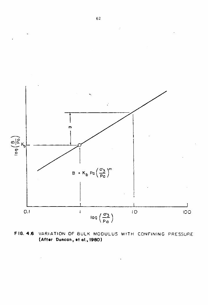
The bulk modulus varies with changes in confining

pressure (03). Hence, to determine the variation of B with

03 the following expression may be used.

In this expression, values for atmospheric pressure (Pa),

confining pressures (03), bulk modulus exponent (m) and

bulk modulus number (Kb) are required. This txpression is

simular to that for defining the variation in values of Ei

resulting from changes in 03 values as presented in

Equation 4.3. For the values of Kb and m, B/Pa versus

03/Pa are plotted on log-log scale as shown in Figure 4.6.

The slope of the line formed represents the value of m and

the Y-intercept, the value of Kb.

4.3 Summary of Results

The determination of hyperbolic parameters for

62

'''.

( 0'"3 )m

B = Kb Po Po

0.1 10 roo

FIG.4.6 VARIATION OF BULK MODULUS WITH CONFINING PRESSURE (Aft er Duncan I et 01. t 1980)

63

both samples tested are included in Appendices Band C; the

results are shown in Tables 4.3 and 4.4. Not surprisingly,

as confining pressure increased the values of Ei and

( ° 1 -03 ) u 1 tal s 0 inc rea sed un d e r bot h t est con d i t ion s . For

the consolidated-drained (CD) test, with a 60 psi increase

in 03, the value of Ei and (01-03)ult increased about four­

fold. Smaller changes in the values of Ei and (01-03)ult

due to similar changes in 3 were recorded for the sample

tested under consolidated-undrained (CU) conditions. For

this case, a 60 psi increase in 03 resulted in an

approximate twofold increase in the values of Ei and

Obviously. the soil type and conditions in

which the soil specimens were tested were the main factors

that caused this difference.

The strength characteristics of the soil types

varied under similar values of

pressure (10 psi), the value of

However, at a 03 value of 70 psi,

03. At low confining

( 01-03 ) u 1 twa s s i mil a r .

the val u e s 0 f ( ° 1-03 ) u 1 t

for soil at the pile tip were almost double that obtained

for the sample which represented soils along the pile

perimeter. The specimen representing soil at the pile tip

exhibi ted a greater internal angle of friction (q,') and

smaller value of cohesion (c') than that obtained for both

the effective and total stress for the specimen

representing soil along the pile perimeter. This is to be

expected since soils at the tip were more granular than

TABLE 4.3 SLMt1ARY OF STRENGl'H AND HYPERBOLIC PARA.i'1ETERS DETE~ INED FOR THE SOl L SA:v1PLES TESTED THAT WERE Q3TAINED fRU1 THE UPPER YOEKTOdN FOR1AT ION

DESCRIPT ION: Fine to med iun sandy clayey sil t, gray (_ Classi fication: t1L

Boring No. B-~ D2pth: 37.5'- 4±t Method: CU - Tr iax ial

°3 (01 -03 ) Cohesion Internal I Ei (psl) (ps i) ul t. c Ang le of Fr iction (psi) Rf

f--(psi) ~

10 34.7 3125 0.58 c = 13 ¢ = 10.50

40 52.0 4348 0.55 c' = 9.5 ¢I = 19. 00

70 62.4 8333 0.61 --------- - ---- ------

Rf avg. 0.58 Ei aV9. 5269 psi

Stratun: Cl

K n

70 O. 5

01 A

TABLE 4~ 4 Slt1MARY OF SrrRENGTH AND HYPERBOLIC PARN'lETE.RS DETERt1INED FOR 'I'HE SOIL SAr1PLES TESTED THAT WERE rnrfAINED FRO'1 THE LCJi.lER YORKTCWN FOFHA'f ION

iDESCRIPf ION: Fine to !l18 3iun sand, some silt, greenish gray Classification SM

[~() ring tb. B

°3 ~ (psi) Hf K n

1 ----

10 33.2 813 0.71 c 4.0 28° 22 0.47

40 .2 1644 0.83 -----

70 104.8 2018 0.79

P. f a vg • 0 .78 Ei 1492 psi

Stratun: C2

(psi) Kb

595 18

1872

1460

m

0.46

0"1 V1

66

those along the pile perimeter.

Th e fa i 1 u r era t i 0 ( R f ) use d tor e 1 ate ( 01-03 ) u 1 t

and (01-03)f varied little with changes in confining

pressure for both test conditions. However, the variation

in values of Rf relative to variation in soil types and

test conditions were significant. For the consolidated-

undrained (CU) condition, a mean Rf value of 0.6 was

obtained and for the consolidated-drained (CD) condition,

the Rf value was 0.8.

Chapter 5

SOIL-CONCRETE INTERFACE TEST PROGRAM

5.0 Introduction

Analysis of soil-structure interaction using the

finite element method requires a knowledge of the stress­

deformation characteristics at the soil-pile interface.

Accordingly, a soil-concrete interface test program was

developed to provide a means of determining the strength­

deformation characteristics along the soil-pile interface.

For the concrete piles analyzed herein, the soil

medium was representative of the upper Yorktown formation

( S t rat um C 1) . The assumption was made that the soils at

the interface undergo remolding during both installation

and loading of the pile. The representative sample was

placed in a remolded state in contact with a precast

concrete block of both smooth and rough surface textures.

Shearing along the soil-concrete interface was accomplished

by a strain-controlled direct shear apparatus.

The objectives of the soil-concrete interface

test program were to determine the strength and hyperbolic

parameters of the soil. The parameters of interest were:

the interface angle of friction adhesion (Ca) ;

initial shear stiffness modulus (Ksi); modulus number (Kj);

and the modulus exponent (n).

67

68

5.1 General Theory

Previous studies have shown that the strength-

deformation characteristics between soil types and solid

surfaces are dependent upon several factors: the physical

properties and gradation of the soil; the moisture content

of the soil and the solid surface; the normal stress;

density of the soil; the material type; and surface texture

of the solid (11).

Utilizing the results of direct shear tests for

numerical solutions require an analytical model of the

shear stress versus the relative displacement curve. As

with the stress-strain curve developed from triaxial tests,

Clough and Duncan (1971) have shown that the stress-

displacement curves from direct shear tests can be

approximated by a hyperbola during primary loading. This

hyperbola can be represented by an equation of the form:

t:.s 5.1

llKsi + ~slT ult

in which is the shear strength, t:.s the relative

displacement, Ksi the initial shear stiffness modulus, and

T u1t representing the ultimate shear strength. The

transformed linear hyperbolic equation of the form shown

below represents a linear relationship between and

h.s.

IJ.s 'T

1 -- + Ksi

69

6s 5.2 " ult

Therefore, to obtain the best fit hyperbola for the stress-

displacement curve, the values of IJ.s/" versus 6s

determined from the test data were plotted. The straight

line which best fits the transformed plot corresponds to

the best fit hyperbola of the stress-displacement curve as

shown in Figure 5.1. Clough and Duncan (1971) have further

shown that the transformed linear hyperbola can be achieved

by a straight line which passes through the points at which

70 and 90 percent of the strength has been mobilized.

Since Equation 5.2 represents that of a straight line, then

the slope and Y-intercept of the transformed hyperbola

represents the inverse values of T ult and

respectively.

The value of the internal angle of friction (~i)

can be determined from the slope of the line which best

fits the plot of " ult versus normal stress (on)' The

shear stress value at failure (Tf) is a function of normal

pressure as expressed by the following equation:

'Tf - on tan 4>i 5.3

The value of "f is smaller than the value of 'T ult and are

related by a factor, referred to as the failure ratio (Rf):

70

"'ult -----~------- - ---

REAL .. Cf) Cf) I&J D: t­Cf)

'" =

D: C( W % en

65

fiGURE 5.1 HYPERBOLIC REPR!SENTATION FOR 01 REeT SHEAR TESTS

TRANSFORMED

A!:...L.+A!. Y' kosi '-.It

71

5.4

This value is similar to the Rf value in Equation 4.2 which

relates ultimate and failure deviatoric stresses derived

from conventional triaxial testing.

The variation of Ksi with un at the interface can

be expressed by the following equation as set forth by

Clough (1969):

5.5

In this equation: ~w represents the unit weight of water;

Pa the atmospheric pressure; Kj the modulus number; and n

the modulus exponent. The values of Kj and n can be found

by first determining the value of Ksi corresponding to the

value of un and plotting the value of Ksi/~w versus un/Pa

on a log-log scale as shown in Figure 5.2. The slope and

Y-intercept of the best-fit straight line through the data

points represents the value of nand Kj respectively.

The relationship of the tangent shear stiffness

modulus (Kst) to the normal stress (un) is represented by

the equation:

1"

tan 5.6

This equation can be used to evaluate the non-linear and

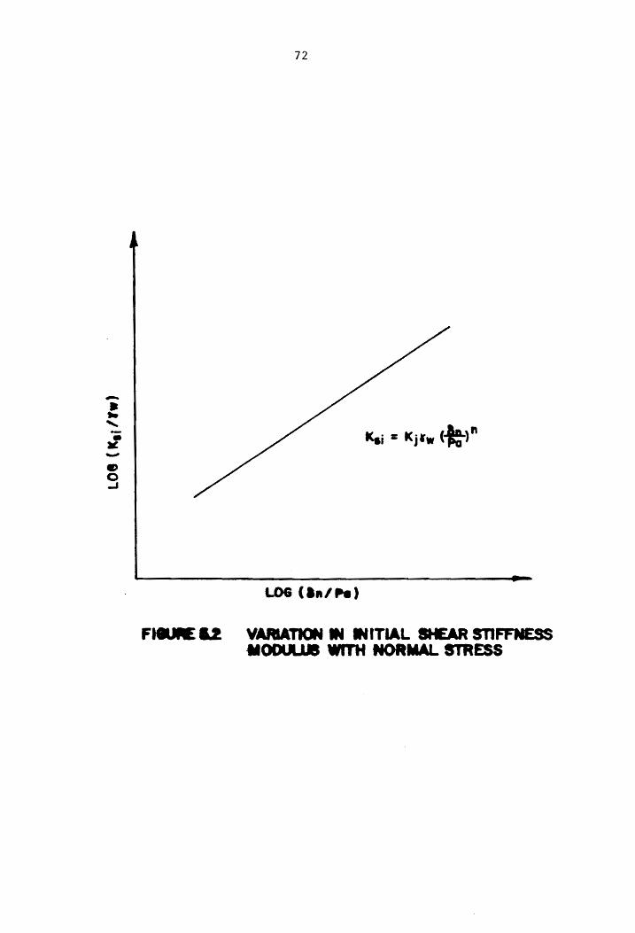
• o -'

72

LOG (a",Pe)

F .... 'E &2 VARIATION .... ITIAL -.AR snFFNESS MODlI .. WITH NORMAL STRESS

73

stress dependent behavior at the interface of the soils in

contact with the solid body_

5.2 Test Apparatus

There are several shear devices which can be

employed for interface testing: the direct shear apparatus

in which the soil undergoes direct single shear along the

zone between the two halfs of a square or circular box; the

double ring shear apparatus which consists of a set of

rings in which the soil can be tested in either direct

single shear or double shear; and finally. the angular

shear device comprised of rings that shear the soil in an

angular manner. These three types of devices are

illustrated in Figure 5.3. The direct shear apparatus was

chosen for use in this test program because it facilitated

sample preparation plus testing and was readily available.

The shear force can be applied to any of the

above devices by two methods. The first involves the

application of a known force and measuring the resultant

deformation; this is referred to as a stress control test.

The second method involves

constant rate and measuring

shearing the sample at

the resul tant force; this

a

is

known as a strain control test. The major advantage of the

strain versus stress control test is that ultimate shear

and peak resistance can be determined more accurately_

74

J o 0---- ------- . __ . D------------'O

DIRECT SHEAR APPARATUS

DOUBLE RING SHEAR APPARATUS

- L-./ I ""'

i ,.. - ...... 1 , ., \

\. " --"

ANNULAR SHEAR APPARATUS

FIGURE 5.3 TYPICAL TYPES OF SHEAR APPARATUS

75

Since this data was necessary in modeling the stress­

deformation behavior of the soil-concrete interface, the

strain control method of testing was employed.

Direct shear interface testing was performed with

a Wykeham-Farrance constant rate strain shear machine,

(Model WF25000), with some minor modifications as

illustrated in Figure 5.4. The machine was able to

accommondate a 4.0 inch square shear box 2.0 inches in

depth and the application of normal stresses up to 5.0 tsf

by means of a loaded hanger arrangement. The specimen was

sheared at a uniform rate of strain through a motor and

gear box arrangement. Twenty-five strain rates, ranging

from 0.0000192 to 0.048 inch per minute, were obtainable.

The shear force was determined by a proving ring in contact

with the upper half of the box.

The motor and gear box arrangement allowed the

shear stress to be applied at a constant rate of strain in

both the forward and reverse directions. The cyclic load

imposed on the soil-structure interface required

modification of the shear box, load piston and proving

ring. The upper portion of the box was attached to the

load piston and to the proving ring which allowed the soil

to be sheared in a forward and reverse direction at a

constant rate of strain.

The shear force in both directions was obtained

by using two Wykeham Farrance proving rings of high tensile

FIGURE 5.4 MODIFIED WYKEHAM-FARRANLE CONSTANT RATE STRAIN SHEAR MACHINE

--.J (j\

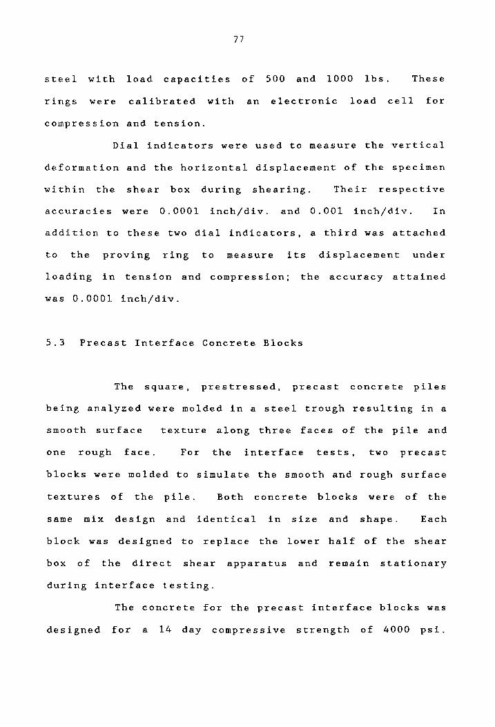
77

steel with load capacities of 500 and 1000 lbs. These

rings were calibrated with an electronic load cell for

compression and tension.

Dial indicators were used to measure the vertical

deformation and the horizontal displacement of the specimen

wi thin the shear box during shearing. Their respective

accuracies were 0.0001 inch/div. and 0.001 inch/div. In

addition to these two dial indicators t a third was attached

to the proving ring to measure its displacement under

loading in tension and compression; the accuracy attained

was 0.0001 inch/div.

5.3 Precast Interface Concrete Blocks

The square, prestressed, precast concrete piles

being analyzed were molded in a steel trough resulting in a

smooth surface texture along three faces of the pile and

one rough face. For the interface tests, two precast

blocks were molded to simulate the smooth and rough surface

textures of the pile. Both concrete blocks were of the

same mix design and identical in size and shape. Each

block was designed to replace the lower half of the shear

box of the direct shear apparatus and remain stationary

during interface testing.

The concrete for the precast interface blocks was

designed for a 14 day compressive strength of 4000 psi.

78

The mix design consisted of Portland Cement, Type IV, with

a water cement ratio of 0.57 and a slump of 4.0 inches.

The fine and coarse aggregate employed in the design mix

consisted of washed sand and crushed limestone

respectively. The 1.0 inch thickness of each precast block

limited the use of aggregate to a size finer than 3/4 inch.

The concrete was placed within wooden molds with

ins ide dimens ions of 4.0 inches square and 1.0 inch in

depth. Two 1/2 inch diameter threaded bolts were embedded

within the concrete block. The threaded ends of the bolt

extended 1.0 inch from the side of the blocks to provide a

means of securing the concrete blocks within the reservoir

of the direct shear device. This precluded slippage during

interface testing. Embedded at the surface of the concrete

block were two metal plates and two threaded shafts

extending the entire thickness of the block. The location

of the plates and shafts corresponded to the threaded holes

located within the upper half of the shear box. The hollow

threaded shafts provided a means of securing the upper half

of the shear box to the concrete block. The slide plate

provided a smooth surface for ease of separating the upper

shear box from the concrete block by use of adjustment

screws.

The desired smooth surface texture of the

concrete was achieved by first troweling to a smooth finish

and placing a glass plate on the surface to further reduce

79

any irregularities. The rough surface texture was obtained

by striking off the concrete with a piece of wood across

the concrete surface. After allowing the concrete to set

for 24 hours within a curing room, the concrete was removed

from the mold, submerged in water and placed back into the

curing room for 14 days.

The strength of the concrete was tested with two

concrete cylinders, 6.0 inches in diameter and 12 inches in

height, that were molded in accordance with ASTM C-3l. The

cylinders were placed in a curing room for 14 days at which

time they were t.ested in accordance with ASTM C-39; the

resultant compressive strength was 3750 psi.

5.4 Soil Selection and Preparation

The samples selected for interface testing

consisted of a mixture of soils from the upper Yorktown

formation. The soil type, moisture content, unit weight,

grain size distribution and Atterberg Limits were

determined since they have an effect on the stress-

deformation behavior at the soil-concrete interface (11).

The sample classified as fine to medium silty

sand with shell fragments (SM) in accordance with ASTM D-

2487. Gradation analysis indicated the soil contained 47

percent material finer by weight than the No. 200 sieve.

The fines exhibited a low plasticity based upon a Liquid

80

Limit of 25 and Plasticity Index of 7.6. By comparison,

laboratory testing of soils from Stratum Cl disclosed a

mean value of 47.3 percent material finer by weight than

the No. 200 sieve.

The moisture content and soil density were based

upon mean values derived from laboratory testing of samples

obtained from various depths within Stratum Cl. The mean

values of the dry and wet unit weight of soils from Stratum

Cl were 96 pcf and 123.2 pcf respectively; the average

moisture content was 28.3 percent. For the latter, air

dried soil was mixed with distilled water, placed in air­

tight bags and allowed to cure for 24 hours within the

moisture room to obtain the desired moisture content.

The soil sample was compacted within the upper

shear box attached to the precast

thereto, the moisture content of

concrete blocks. Prior

each tes t spec imen was

determined. Based on the moisture content of the sample

and the volume of the upper shear box, a predetermined

weight of soil sample was used. The soil was uniformily

compacted to the desired wet and dry soil density of

approximately 96 and 123 pcf respectively.

5.5 Interface Testing Procedures

Basically, direct shear interface testing

involves three phases: preparation of the soil sample;

81

load application plus soil consolidation; and shearing of

the specimen. The procedures that were followed for each

of these phases are enumerated below:

Phase 1: Soil Preparation:

a. The upper half of the shear box was attached

to the precast block using clamp screws.

b. The soil was compacted to the desired density

within the upper half of the box; care was taken to assure

that the soil was compacted uniformly and that the box was

completely filled.

c. Filter paper was placed over the soil and

trimmed to the ins ide dimensions of the box; a square

porus stone and loading cap was placed on top of the paper.

Phase 2: Loading and Consolidation of Soil:

a. The concrete-shear box assembly was

to the direct positioned within the reservoir attached

shear apparatus; the concrete block was secured within the

reservoir by adjusting the hex nuts on

extending from the side of the block.

movement of the block during testing.

the threaded bolts

This prevented any

In placing the

assembly within the

arm attached to the

reservoir, the key socket on the load

upper half of the shear box had to

slide over the key attached to the load ring; the assembly

was then secured with the hex nut.

82

b. The load hanger, ball and yoke were

positioned on top of the loading cap and the desired load

applied to the hanger. Dial guages were attached to

measure vertical and horizontal displacements as

illustrated in Figure 5.5. The clamp screws which secured

the shear box to the concrete block were removed and the

spacing screws separating the upper shear box from the

concrete block were adjusted. The separation distance

corresponded to the largest grain size of the soil specimen

and was measured with a feeler guage.

c. The four screws securing the load cap to the

upper shear box were loosened and readings of vertical

displacement were taken. The spacing screws were then

removed and the reservoir was filled with distilled water.

d. Time readings of vertical displacement were

continued; once secondary consolidation occurred, the

sample was considered ready for shearing.

Phase 3: Shearing of Soil Specimen:

a. During shearing of the specimen, readings

were taken of vertical movement with corresponding load

ring readings at intervals of 0.005 inch of horizontal

displacement until failure occured.

b. Once failure occured, the direction of shear

was reversed and readings on all three guages were taken as

in 3a above until the shear box returned to its original

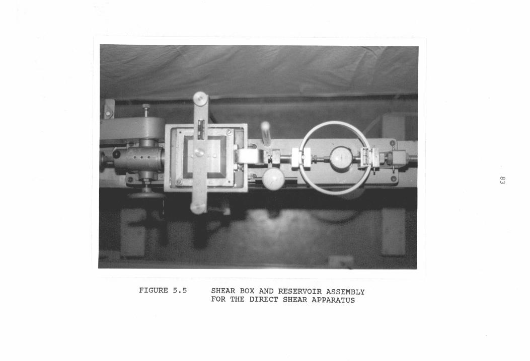
FIGURE 5.5 SHEAR BOX AND RESERVOIR ASSEMBLY FOR THE DIRECT SHEAR APPARATUS

00 w

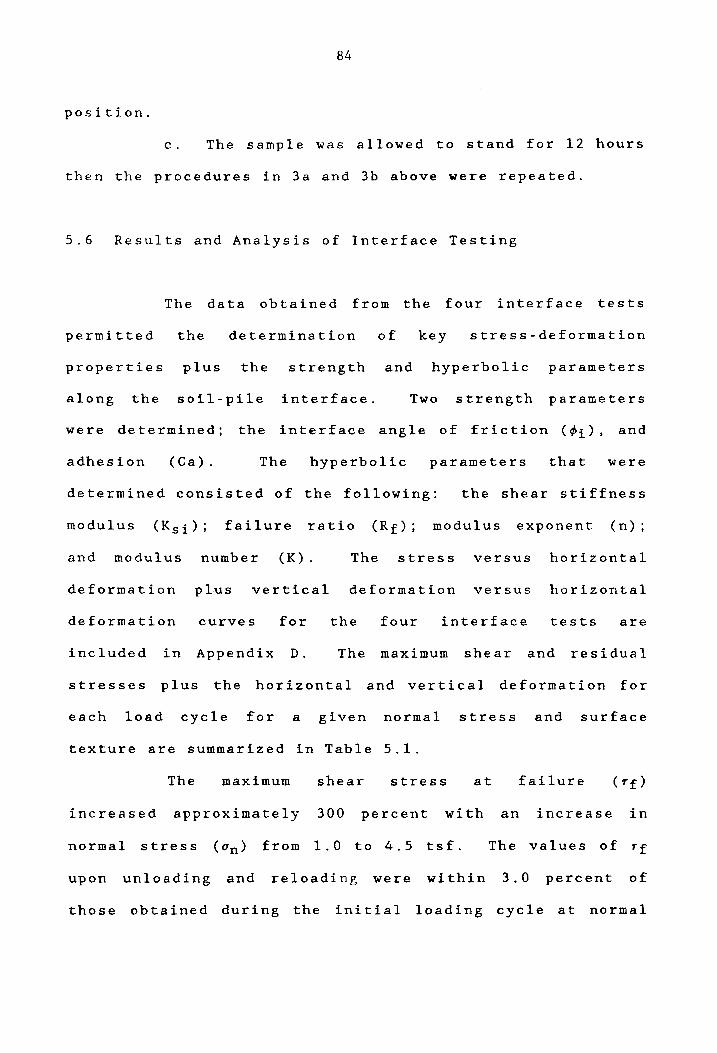
84

position.

c. The sample was allowed to stand for 12 hours

then the procedures in 3a and 3b above were repeated.

5.6 Results and Analysis of Interface Testing

The data obtained from the four interface tests

permitted the determination of key stress-deformation

properties plus the strength and hyperbolic parameters

along the soil-pile interface. Two strength parameters

were determined; the interface angle of friction (~i)' and

adhesion (Ca). The hyperbolic parameters that were

determined consisted of the following: the shear stiffness

modulus (Ksi); failure ratio (Rf); modulus exponent (n);

and modulus number (K). The stress versus horizontal

deformation plus vertical deformation versus horizontal

deformation curves for the four interface tests are

included in Appendix D. The maximum shear and residual

stresses plus the horizontal and vertical deformation for

each load cycle for a given normal stress and surface

texture are summarized in Table 5.1.

The maximum shear stress at failure

increased approximately 300 percent with an increase in

normal stress (un) from 1.0 to 4.5 tsf. The values of 1'f

upon unloading and reloading were within 3.0 percent of

those obtained during the initial loading cycle at normal

Test Cycle

Load

Unload

Reload

Unload After 12 Hrs

Reload After 12 Hrs

TABLE 5.1 RELATIONSHIP OF NORMAL STRESS VERSUS HORIZONTAL AND VERTICAL DEFORMhTION

Smooth Surface

Stress-Defonmation Parameters 1 2 3

Maximum shear stress (Tf)' psi 13.15 24.04 40.22 Horizontal displacement ~ Hf>, in 0.185 0.30 0.475 Vertical displacement (6Vf>, in 0.00510 0.0196 0.0314 Resldual shear stress (Tr) 13.06 23.95 Horizontal displacement (6Hr) 0.210 0.320 N/A vertical displacement (6vr) 0.00545 0.0203 Shear stress (TU) 0 0 0 Horizontal displacement (6Hu) -0.118 -0.06 -0.87 vertical displacement (6vu) 0.0082 0.0063 -Maxlmum shear stress (Tf') 4.291 24.59 38.91 Horizontal displacement (6Hf') -0.325 -0.320 -0.425 vertical displacement (~vf') 0.01035 0.0268 0.0308 Residual shear stress (Trl) 4.278 Horizontal displacement (~Hr') -0.350 N/A N/A vertical displacement (~vr') 0.01035 Shear stress (TU') 0 0 0 Horizontal displacement (6Hu') 0.015 0.064 0.010 Vertical displacement (6vu') 0.0006 0.00445 0.0044 Maximun shear stress (T fn) 13.03 23.90 40.32 Horizontal displacement (~Hf") 0.235 0.345 0.400 Vertical displacement (~vf") 0.0067 0.0084 0.0104 ReSIdual shear stress (T rtl) 12.80 23.84 Horizontal displacement (6Hr") 0.40 0.350 N/A Vertical displacem~nt (~yr") 0.0067 0.0084

- .

Rough Surface

4

24.02 0.275 0.0226

N/A

0 -0.06

0.0025 23.67 0.30

0.0422

N/A

0 0.076 0.0039

25.30 0.270 0.00698

25.0 0.325 0.0068

00 Ln

86

stresses of 2.7 and 4.5 tsf. For the sample sheared at a

normal stress of 1.0 tsf, the value of 'rf upon reloading

was 67 percent of that obtained during the initial load

cycle. At the end of the reload cycle, shearing of

specimens was suspended for a period of 12 hours. After

the 12 hour hold period, the test specimens were subjected

to cyclic loads. The values of 'rf obtained during this

reloading cycle were within 0.9 percent of the value of Tf

recorded for the initial load cycle.

The interface stress-deformation characteristics

resulting from changes in the concrete surface texture were

only available for interface tests conducted under a normal

stress of 2.7 tsf. During the initial loading cycle,

values of maximum shear strength of 24.04 psi and 24.02 psi

were recorded for the smooth and rough surfaces

respectively. Upon unloading and reloading the value of Tf

for the rough surface was 3.7 percent less than that

obtained for the smooth textured block. The value of Tf

upon unloading and reloading the test specimens at the end

of the 12 hour hold period was 5.5 percent greater.

Strength parameters were determined from the

stress-deformation data obtained from the three smooth

surface interface tests during initial loading. The values

of maximum shear stress at failure (Tf) versus normal

stress (un) for each test are plotted in Figure 5.6. From

the slope and Y-intercept of the line which best fits the

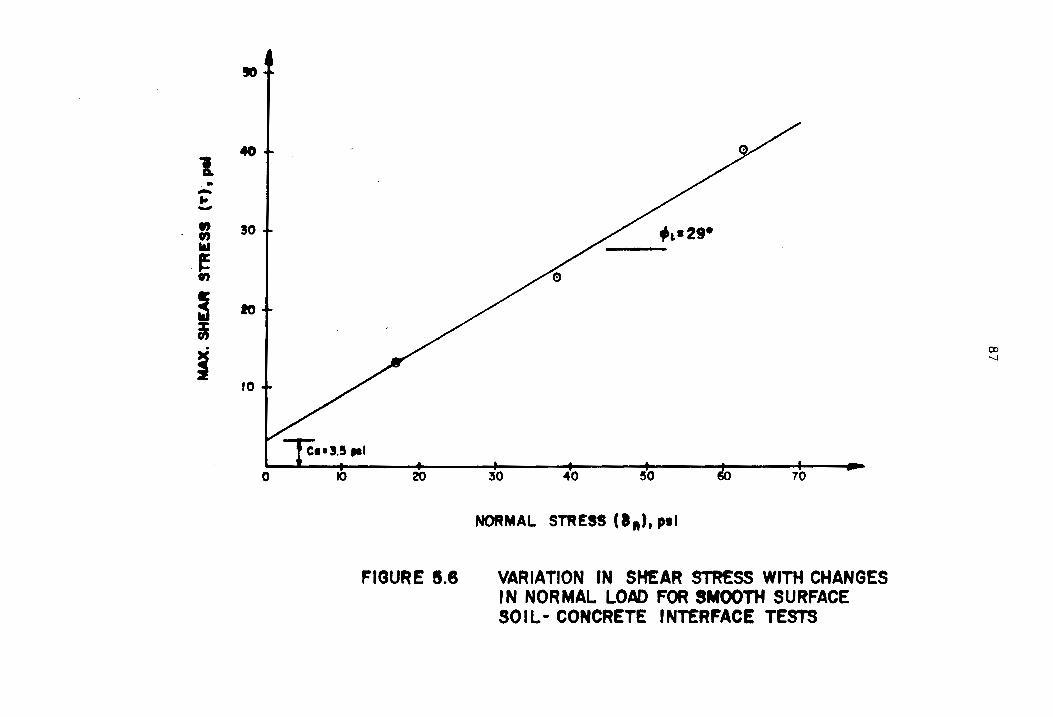
!IO

1 40

• ....... .. .....,

• 30 t en ... ~ en

! 10

i

i fO

o

../'

10 20

FIGURE 5.8

/' .,,-29-

30 40 50

NORMAL STRESS (I,,), Plf

VARIATION IN SHEAR STRESS WITH CHANGES IN NORMAL LOAD FOR SMOOTH SURFACE SOIL-CONCRETE INTERFACE TESTS

ex> ........

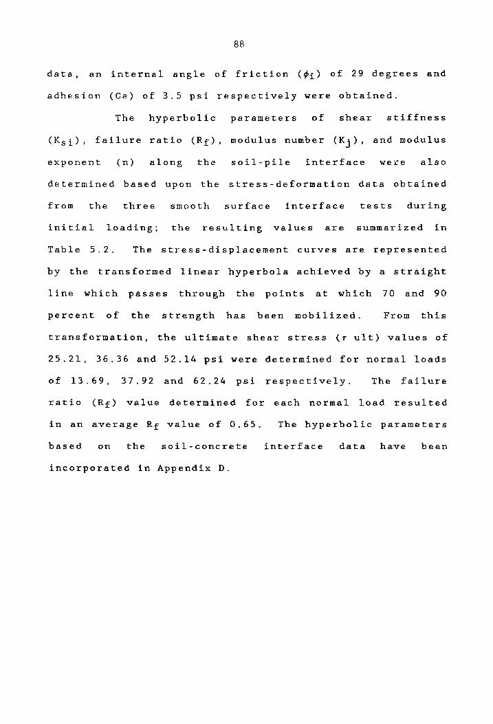
88

data, an internal angle of friction (¢i) of 29 degrees and

adhesion (Ca) of 3.5 psi respectively were obtained.

The hyperbolic parameters of shear stiffness

(Ksi), failure ratio (Rf), modulus number (Kj), and modulus

exponent (n) along the soil-pile interface were also

determined based upon the stress-deformation data obtained

from the three smooth surface interface tests during

ini tial loading; the resul ting values are summarized in

Table 5.2. The stress-displacement curves are represented

by the transformed linear hyperbola achieved by a straight

line which passes through the points at which 70 and 90

percent of the strength has been mobilized. From this

transformation, the ultimate shear stress (T ult) values of

25.21, 36.36 and 52.14 psi were determined for normal loads

of 13.69, 37.92 and 62.24 psi respectively. The failure

ratio (Rf) value determined for each normal load resulted

in an

based

average Rf value of 0.65.

on the soil-concrete

incorporated in Appendix D.

The hyperbolic parameters

interface data have been

TABLE 5.2 SU'1f1ARY OF HYPERBOLIC PARAt1E'rERS DETER1INED FRQ'1 SOIL-CON2RETE INTERFlCE TESTING

Fine to medium silty sand with . . DEs:::rUPfrON: shell fragments, gray flcatlon: SM Stratun: Cl

f3c;[ 00. 8-1 14.5'- 60' r~thod: t Shear Interface Testing

()11 n Ks (ps ) e of Friction (psi) n

<Pi

13.7 3.2 0.52 3.5 29° 270 0.34

37. 2:1.0 0.66

62.2 0.2 360 0.77

Ks

co 1..0

Chapter 6

FINITE ELEMENT METHOD OF ANALYSIS

6.0 General

Finite element analysis of Geotechnical

engineering problems has obtained greater acceptance with

the growth in computer technology and the reduction of

computer costs. Among its uses in this field are the

analyses of deep foundation systems. Conventional methods

for this purpose include: dynamic and static formulas;

empirical static formulas based upon liN" values; and wave

equations. These are designed to compute deformation and

bearing capacity of piles t however, they generally cannot

account for many of the variables that affect pile capacity

and behavior. As noted earlier, in this category are: in-

situ stresses; soil disturbance and induced stresses caused

by pile driving; variations in soil strength and soil-pile

interface properties;

friction plus cyclic

consolidation

load. In this

and negative skin

regard, the fini te

element method has shown promise in handling many of these

factors.

In this study, the application of the finite

element method was used to ascertain the pile capacity and

the behavior of a single concrete pile modeled after the

piles and subsurface conditions at the Land Level

90

91

Shipbuilding Facility in Newport News, Virginia. The data

derived therefrom permitted a comparative analysis to be

made with the results from full scale pile tests conducted

at that location. Essential to this undertaking was the

determination of the soil strength-deformation

characteristics and hyperbolic parameters of the soil media

in which piles at this site are embedded. In addition, the

strength-deformation characteristic and hyperbolic

parameters along the soil-pile interface are required.

The program used for the analysis was the "soil-

struct" axi-symmetric finite

(1982) (4) . The parameters

element

that were

program

obtained

by Clough

from this

program included: the ultimate bearing capacity; the load­

deformation behavior; and load-transfer characteristics of

the pile.

6.1 Finite Element Procedures

Described below in outline fashion are the basic

steps involved in

These steps were

for this study_

the finite element method of analysis.

also followed in the

Details regarding

analysis performed

applications and

procedures for the solution of various engineering problems

are well documented in various publications (7,21).

The finite element method of analysis generally

consists of five basic steps,.

92

Step 1 - Discretization:

This initial step, as implied hy the term,

segments the region to be analyzed. In addition to

segmenting the regiort, the boundary of the region is also

delineated. In this study, the boundary was defined as the

limits within the soil medium which are not affected by

pile loading. The concrete pile and soil medium within the

specified boundary were incorporated into a finite element

mesh. Two types of "elements" were used: the two

dimensional quadrilateral and the interface.

The two dimensional guadrilateral element (QMS)

was developed hy Doherty, Wilson and Taylor (1969). The

shape of this element is shown in Figure 6.la. It has four

corner nodes plus an internal condensed node and was used

to discretize the pile and the soil medium. The interface

element allows for simulating movement at the junction

between the pile and surrounding soil medium; it was

defined by four nodes. Each of two pairs of nodes were

assigned the same coordinates; thus, the interface element

had no thickness as illustrated in Figure 6.lh.

Each element of the mesh is assigned various

physical properties and its stiffness equation formulated.

The individual elements are then aggregated to obtain the

equations for the total structure being analyzed.

..

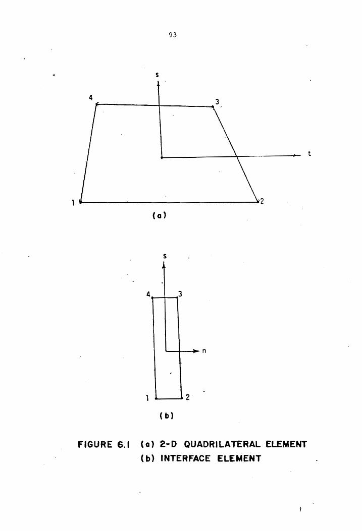
93

s

4 r--------4 ______ ~3

1 IJ-----------------~.

(a)

S

J

4 3

(b)

::- n

FIGURE 6.1 (a) 2-D QUADRILATERAL ELEMENT

( b) INTERFACE ELEMENT

t

94

Step 2 - Selection of Approximation Functions:

In a two dimensional analysis, the displacement

within each element can be expressed as follows:

- [N] {q} 6.1

where: u displacement in the x direction

v displacement in the y direction

{q} nodal displacement vector

[N) matrix of approximation function

Both the displacement and geometry of the element are

expressed by using the same matrix of approximation

function, [N], which is dependent upon the type of element

used in the analysis. Descriptions of various matrix of

approximation functions corresponding to different types of

elements are discussed by Doherty, Wilson and Taylor

(1969).

Step 3 - Derivation of she Element Eguations:

Using variational theory or the weighted residual

method, the element stiffness equation is derived as

follows:

(k] {q} - {Ql 6.2

In this relationship, (k] is the element stiffness matrix

95

which is determined from the following equation:

[k] - fffv [B]t[c] [B]dv 6.3

where: { q } nodal displacement vector

{Q} load vector

[c] constitutive matrix

(B] transformation matrix

v volume of the element

The constitutive matrix [c] is obtained from the

stress-strain behavior of the soil. For soils along the

pile perimeter and pile tip, hyperbolic stress-strain

relations are used in which the tangent Young's Modulus

(E t ) is changed for each load step of the calculation using

the following formula:

6.4

Determination of non-linear stress dependent behavior at

the soil-pile interface is based on the tangent shear

stiffness modulus (Kst ); it is determined using Equation

6.5 which was also discussed in Chapter 5.

6.5

96

Step 4 Assembling Element Properties To Form Global

Eguations:

In the previous step, Equation 6.3 was obtained

for each element in the structure. In this step, these

equations are combined to form a stiffness relationship for

the entire system by adding the matrix equation for each

element in the following manner:

where:

[K] {r} - {R}

[ K]

{ r}

{R}

global stiffness matrix

global nodal displacement vector

global nodal force vector

6.6

Before the set of simultaneous equations can be

solved, the geometric boundary conditions are introduced

into the system.

Step 5 - Solve For The Primary And Secondary Unknowns:

The nodal displacement {r} represents the primary

unknown and is computed by Equation 6.6. The secondary

unknown stress (a) and strain (E) within each element can

be found using the following relationships wherein the

vector of nodal displacement, (q), is known.

tE} - [BJ {q} 6.7

97

and:

fa} - [c] {El - [c] [B] {q} 6.8

6.2 Application and Results

The soil strata and pile type were modified for

ease of application of the finite element method. The 14

inch square concrete pile was simulated by an equivalent

circular pile with a tip and butt diameter of 15.84 inches.

The model pile in this analysis assumed a 60 feet embedment

within the Yorktown formation. For the actual case, only

42 and 44 feet of the total embedment length of test piles

TP-3 and TP-4 respectively were embedded within the

Yorktown formation. This simulation was considered

reasonable since the Norfolk formation was found to

contribute little to the bearing capacity of the piles.

The soil strata plus pile embedment of the test

and model piles are depicted in Figure 6.2. The surface

area at the pile tip and pile perimeter of the actual

versus the model pile is presented in Table 6.1. The

additional surface area along the pile perimeter resulting

from deeper simulated embedment of the model pile in the

Yorktown formation was introduced to account for the

capacity attributed to the Norfolk formation in the case of

the test piles.

The finite element mesh that was used to analyze

98

0 0 0 0 0 0 0 0 N It') V 10 CD ,....

0..1

w .-:1 -l 1IJ1

a:: =1 0.. 1 -l W 0 0 :l:

if) W

NM01)f~OA ~3ddn NM01)f~OA ~

~3MOl lJ... 0 n:: D-

~ a.. Z

V W I I- 2 a.. 1IJ 0 ...... ..J

W w m .J ~ a.. W

...... U) W w ~ ......

)fl O~ ijON NM01)f~OA ~3ddn I NM01)f~OA ~3MO' Q /111~

1

(\J

c.6 a.. W

I'f) I- 0::::

I => a.. 1IJ ...... .J (9

n: w LL

.J

a.. I

...... I CJ) I w I

.. J.., ...... -I"'" I

1 NM01)f~OA H3ddn NM(1)fijOA

I I ~3MOl

0 0 0 0 0 a 0 0 N ,..., V 10 <D ,....

( .~ I ) , Hld 30

TABLE 6.1 PILE SURFACE AREA, FT2

Test Pile Test Pile TP-3 TP-4

Pile Tip 1.4 1.4

TOtal Pile Perimeter 284.7 270.7

PIle Peruneter Embedded in the Yorktown Fonmation 196.0 205.3

Model Pile

1.4

248.8

248.8 \0 \0

100

the behavior of the soil and model pile is shown in Figure

6.3. It consisted of 293 nodes and 285 elements, 16 of

which were interface elements. Four-node quadrilateral

elements were used to discretize both the soil medium and

the pile. At the interface of the pile and the surrounding

soil medium, interface elements were used. Table 6.2 gives

the material properties for the soil medium and the pile;

the soil-pile interface properties are given in Table 6.3.

The pile was loaded in 30 ton increments to a

maximum load of 300 tons. This corresponds to the maximum

load obtainable in the pile load test. Before applying the

load, the in-situ stresses were set-up in the soil plus the

interface and pile elements. Initial stresses in the

interface and the pile elements were set equal to those in

the adjacent soil elements. The initial shear stress for

all elements along the ground surface were set equal to

zero.

6.3 Analysis of Results

The applied load versus pile butt displacement

was determined at various increments by finite element

analysis and compared with load-displacement data obtained

from the pile load tests performed on test piles TP-3 and

TP - 4. The resu1 ts are shown in Figure 6.4. The load­

displacement response resulting from the model pile was

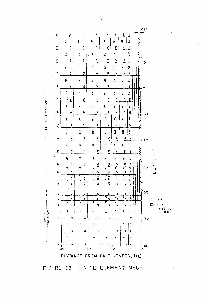
101

0.66'

---.,.------_ ~ r. ~ ~ e; ~ ~ ~

t ~ '---1 F..L,--~E ~t.L+--~--I:E,,-+--~~ r;1~~ l""-l1_ -C<~ ;.....f.-l'~~ll+lr ~-,>I I V 1£ i" ~ I~ ~ ~ I ~ 1-----...t-4..~__:....1 --J;.~'-l--_LLt-~----.J:,~yl-----LJ.~-+--""'-:.£',-~s."-+++4A-~ - 10

cr:: Lu 0... 0... ::)

! V 8 ~ ~ 6 E ~ v

~ ~I---~~--~~~~~~~~+-~~~~~~~+H~

g ~ !! I ~ ~ ~I-l."l N N N N

~~-:~~4---~~--~~~~E~~~Y-~~~~~4/~20 ~ ~ ~ ~ ~ 2

II' r- 1;:1 1/1 N ~

~~~~y-__ ~~~ __ ~~ __ ~~~+-~~m+-~~~~-+H~~vl-~< Sf

I

<~~~'~~~--~~~~~~~--~~=+-~'~+-~~~~4+~30

I ~

V

r

<0 &3 !-

#r-~:~.~~·r-~~y-__ ~ffiY-~~~~~~~~~~~-HV~

~ ~ lIB ~

o I j

In

v

80 o

DISTANCE FROM PILE CENTER, (tt.)

FIGURE 6.3 FINITE ELEMENT MESH

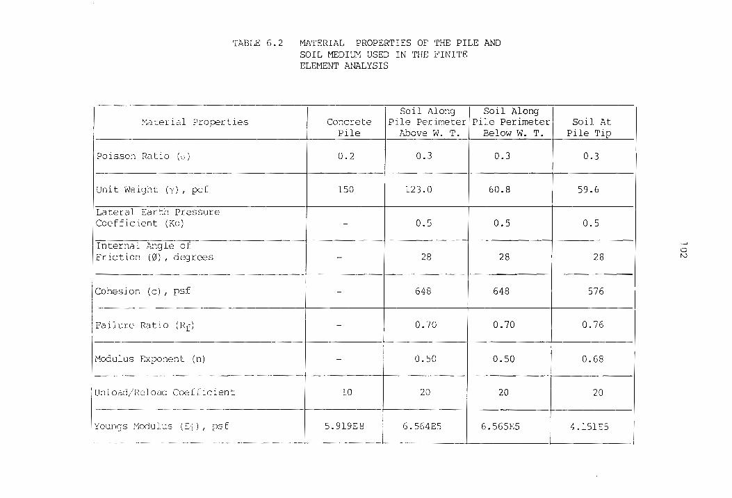
TABLE 6.2 MATERIAL PROPERTIES OF THE PILE AND SOIL MEDIUM USED IN THE FINITE ELEMENT ANALYSIS

1 Al 1 .1i l"Jd ter ial Properties Concrete Ie Perimeter Pile Perimeter

Pile Above W. T. Below W. T.

Poisson Ratio (v) 0.2 0.3 0.3

unit Weight (y), pef 150 123.0 60.8

Late 11 E, th Pressure ient (Ko) - 0.5 0.5

lite. .1 Angi If Friction (~), degrees - 28 28

Cohesion (c), - 648 648

Failure Ratio (Rf) - 0.70 0.70

Modulus Exponent (n) - 0.50 0.50

CC><2f icient 10 20 20

MexJulus ( ) f 5.919E8 6.564E5 6.565E5

Soil At Pile Tip

0.3

59.6

0.5

28

576

0.76

0.68

20

4.151E5

-

I-' o f'0

TABLE 6.3 MATERIAL PROPERTIES AT THE SOIL/PILE INTERFACE USED IN THE FINITE ELEMENT ANALYSIS

IShear Stiffness (Ks), psf 6.S64ES

Cohesion (e), pcf 0

Internal Angle of Friction (~), degees 28

Tensile Strength, psf 0.10

Strength Factor (Rf) 0.69

~

o w

o

0.2

0.4

,... 0.45 tn lLI J: U Z 0.8 ........

... Z LIJ 1.0 2 LIJ .... ... 1.2

ti ., 1.4

1.8

1.8

2.0 o

Ou'220TONS

Qu t 250 TONS

o 'ILE T-'

ll. ''If T-4 [:] MOD! l " L!

SLOPE' 0.05" /TON (0.014 CM/KN)

400 100 200 300 LOAD (TOIt)

FIGURE 6.4 LOAD- SETTLEMENT CURVES FOR THE MODEL PILE AND TEST PILES TP-! AND TP-4

500

...... o p.

105

similar to that exhibited by test pile TP-3 to within 0.1

inches throughout the initial load cycle to failure. Test

pile TP-4 exhibited less displacement at the pile butt

compared to both test pile TP-3 and the model pile. As

previously discussed, difficulties were encounted during

the load test with pile TP-4 and resulted in pre loading and

subsequent redriving prior to load testing. In addition,

pile TP-4 was embedded about five feet within the firm

granular soils of the lower Yorktown formation whereas test

pile TP-3 was embedded in the soft fine grain soils of the

upper Yorktown formation only. This was also the simulated

case for the model pile. Due to the above condi tions,

greater amounts of compressive residual loads may have

developed at the pile tip prior to load testing compared to

test pile TP-3 and the model pile. This would result in

less measureable displacement for a given load up to plunge

failure.

The ultimate capacity of the model and test piles

were determined by the Norlund method (15). This resulted

in the following ultimate bearing capacity values: 235 tons

for the model pile; 250 tons for TP - 3; and 220 tons for

test pile TP-4.

The ultimate load capacity of the model pile was

also determined by general static analysis. The static

analysis which was used employed soil mechanics and bearing

capacity theory for determining the ultimate load capacity

106

of a single pile from measured soil properties. The

ultimate load capacity of a single pile (P u ) is generally

expressed as the sum of the ultimate pile shaft resistance

(P su ) plus ultimate base resistance (Pbu) minus the weight

of the pile (Wp) as shown below:

6.9

The ultimate base resistance (Pbu) is defined by Vesic

(1975) by the following expression.

6.10

where:

Ab cross-sectional area of the pile tip

c - cohesion

q mean normal ground stress

Nq bearing capacity factor

Nc * - bearing capacity factor

The value of the mean normal ground stress (q) is a

function of the at-rest lateral earth pressure (Ko) and

ver:tical stress (qv)' It is determined by the following

equation:

1 +3 2Ko (qv) 6.11

Vesic (1975) established that bearing capacity factors are

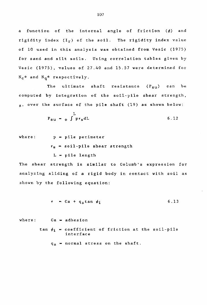
107

a function of the internal angle of friction (¢) and

rigidity index (Ir) of the soil. The rigidity index value

of 10 used in this analysis was obtained from Vesic (1975)

for sand and silt soils. Using correlation tables given by

Vesic (1975), values of 27.40 and 15.57 were determined for

Nc * and Nq* respectively.

The ultimate shaft resistance can be

computed by integration of the soil-pile shear strength,

slover the surface of the pile shaft (19) as shown below:

L Psu - a J p"'sdL 6.12

where: p pile perimeter

"'s soil-pile shear strength

L pile length

The shear strength is similar to Columb' s expression for

analyzing sliding of a rigid body in contact with soil as

shown by the following equation:

where: Ca

tan tPi

6.13

adhesion

coefficient of friction at the soil-pile interface

qs - normal stress on the shaft.

108

The normal stress on the shaft (qs) is equal to the

vertical stress (qv) multipled by a coefficient of skin

pressure which is similar to the at-rest earth

pressure coefficient (Ko).

Based upon the statistical method of analysis

described above and use of the soil properties given in

Table 6.2, ultimate shaft and base resistance values of 145

tons and 47 tons respectively were computed for the model

pile. Neglecting the weight of the pile, the ultimate load

capacity of the model pile was 192 tons. This is a

conservative estimate of pile capacity as compared to the

results from both the finite element analysis and pile load

tests.

In the finite element method, the stress at the

centroid of each element that constituted the model pile

were determined for each load increment. The load-

distribution curves developed from these data at applied

loads of 60, 150 and 210 tons are presented in Figure 6.5.

Load distribution curves that were developed for test piles

TP-3 and TP-4 are also presented in Figure 6.5.

At

distribution

an applied load

curves exhibited by

of 150 tons,

the model pile

the load-

and test

pile TP-4 were similar; whereas, a greater variance

resulted for test pile TP-3. Variations of the load-

distribution curve of the model pile compared with those of

the test piles are attributed to the fill and soils of the

109

LOA 0 (toni) 100 150 200 250

O......-----<;l-i l-----+----~----~ ~--~

-.... :::t: ....

10

20

30

a.. 40 I.J..J o

50

o MODEL PI LE 8 PI LE TP-:-4 o PILE TP-3

60 ..

FIGURE 6.5 LOAD- DISTRIBUTION CURVES FOR THE MODEL PILE AND TEST PILES TP-3 AND TP-4

110

Norfolk formation which contributed little to capacity and

therefore were not considered in the model case. In

addition, the differences may have resulted from residual

stresses

was not

developed during driving of the

considered in the finite element

test piles. which

method. It is

possible to account for such residual stresses in the

finite element method of analysis but this was not

attempted.

The degree of correlation between the model pile

and actual pile behavior are further illustrated in Figure

6.6 by a plot of the applied load mobilized as point and

side friction resistance throughout the initial load cycle.

The shear stress recorded for each interface element was

divided by the surface area of the pile segment for each

element and summed to obtain the shaft resistant values

presented. The tip resistance is the difference between

the shaft resistance and gross load applied. The general

trend of each curve is similar indicating a greater

percentage of the applied load is maintained by shaft

resistance than by tip resistance with all three curves

linearly increasing at a porportiona1 rate up to about 210

tons. Beyond the 210 ton load, the percent mobilized at

the pile tip increased at a higher rate than along the pile

perimeter.

The percentage of load mobilized as shaft and tip

resistence for the model pile and test pile TP-3 were

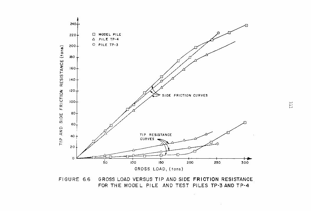
o MODEL PILE

8 PILE TP-4

200 J o PI LE TP-3 • c 0 - 180 w u Z 160 <:( ~ (f)

(f) 140 W a::: Z 120 0 I /7 ~ SIDE FRICTION CURVES ~ u

lOOT // - I--' a::: I--'

LL I--'

W 80 0

CJ) 60

0 2: « 40+ _# TI P RESISTANCE Q.. CURVES -I-

20

0 I

50 100 150 200 250 300

GROSS LOAD I (tons)

FI GU RE 6.6 G ROSS LOAD VERSUS TI P AND 51 DE FR I eTION RESISTANCE FOR TH E MODE L PI LE AND TEST PILES TP"3 AND TP-4

112

similar. When compared to test pile TP-4, a slightly lower

percentage of load was mobilized as shaft resistance and a

higher percentage as tip resistance. This difference is

believed to be the result of additional side friction

resistance derived from the additional surface area within

the bearing stratum of the model and test pile TP-3 as

compared with test pile TP-4.

The percentage of shaft resistance and tip

resistance mobilized at the limit load for the test piles

and the model pile determined from both the finite element

method and static analysis are shown in Table 6.4. The

percentage of shaft resistance mobilized at the limit load

for test pile TP-3 and the model pile were similar. Test

pile TP-4 contained less shaft resistance and greater tip

resistance at the limit load as compared with the other two

cases, This may be the result of the embedment of pile TP-

4 in the granular soi Is of the lower Yorktown forma tion.

The static analysis used to compute the ultimate load

capacity of the model pile described herein resulted in a

greater percentage of tip resistance and less shaft

resistance mobilized at the limit load than was determined

by the fini te element analys is. In the finite element

analysis, the initial Young's Modules was used for soils at

the pile tip. Due to pile driving, the soils at the tip

are subj ec ted to load/unload condi tions . Therefore, the

use of the unload/reload modulus value may be better suited

TABLE 6.4

TEST PILE TP-3

TEST PILE TP-4

MODEL PILE BY FINITE ELEMENT ANALYSIS

MODEL PILE BY STATIC ANALYSIS

113

PERCENT SHAFT AND TIP RESISTANCE MOBILIZED AT THE LIMIT LOAD FOR TEST PILE TP-3, TP-4, AND THE MODEL PILE

SHAFT TIP LIMIT LOAD RESISTANCE RESISTANCE

(TONS) (%) (%)

250 90 10

220 82 18

235 89 11

192 76 24

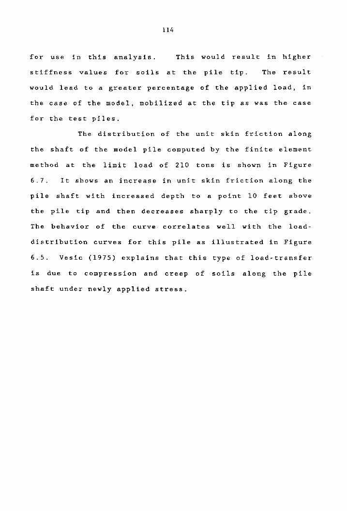
114

for use in this analysis. This would result in higher

stiffness values for soils at the pile tip. The result

would lead to a greater percentage of the applied load, in

the case of the model, mobilized at the tip as was the case

for the test piles.

The distribution of the unit skin friction along

the shaft of the model pile computed by the finite element

method at the limit load of 210 tons is shown in Figure

6 . 7 • It shows an increase in unit skin friction along the

pile shaft with increased depth to a point 10 feet above

the pile tip and then decreases sharply to the tip grade.

The behavior of the curve correlates well with the load­

distribution curves for this pile as illustrated in Figure

6.5. Vesic (1975) explains that this type of load-transfer

is due to compression and creep of soils along the pile

shaft under newly applied stress.

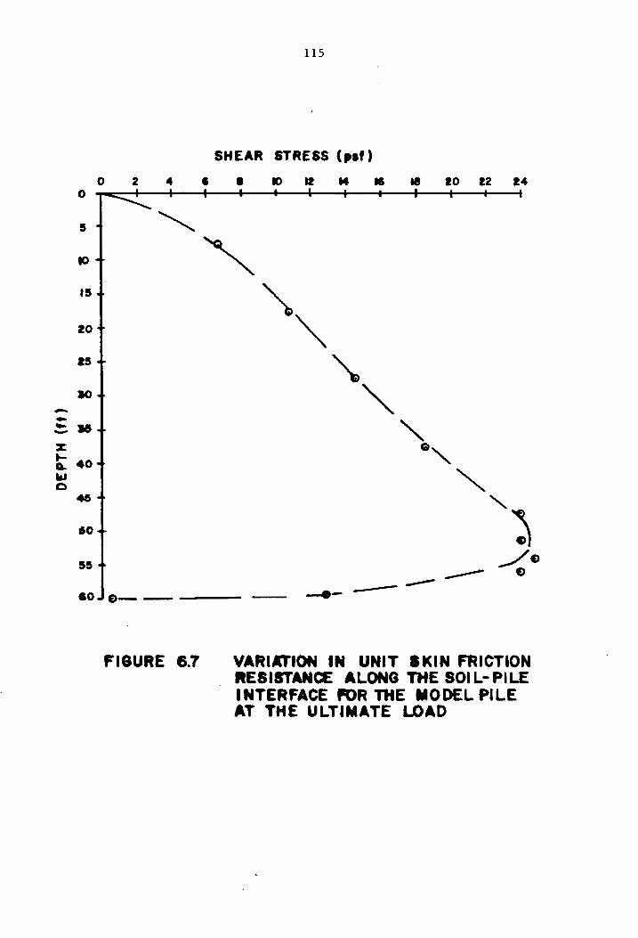
115

SHEAR STRESS (,If)

0 2 4 • • 10 12 M • Ie to 12 14 0

5

10

15

20

H

.a --. ... !:.. %

t:: 40 .... 0

4S

60

55

.0 e- _ --- - --e-

FIGURE 6.7 VARIATION IN UNIT SKIN FRICTION RESISTANCE ALONG THE SOIL-PILE INTERFACE fIOR THE MODEL PILE AT THE ULTIMATE LOAD

7.0 Summary

CHAPTER 7

SUMMARY AND CONCLUSIONS

The finite element method was used to determine

the load-capacity and behavior of a single concrete pile

that was modeled after full scale instrumented piles used

during the design phase of the foundation system for the

Land Level Shipbuilding Facility located in Newport News,

Virginia. The principal function of this facility is the

construction of Naval ships and submarines. Hence, the

foundation was

large area.

designed for heavy loads over

The final design involved

an extremely

over 10,000

prestressed precast concrete piles capable of handling 100

tons each.

The objective of the study was to compare the

results obtained from the finite element method with those

derived from full scale pile load tests that were conducted

for the Shipbuilding Facility. The outcome of this

comparative analysis formed the basis for assessing the

feasibility and effectiveness of the finite element method

in the design of deep foundation systems in the Tidewater

area of Virginia.

Before the comparative analysis could be

accomplished, it was necessary to ascertain the subsurface

116

117

conditions in the immediate vicinity of the test piles.

Moreover, the conditions and manner in which the pile test

program was conducted was of extreme importance. All

available information relevant to this aspect of the study

was addressed.

Despite the extensive soil investigative program

undertaken by the design firm for the foundation, the data

generated did not provide all the soil parameters required

for the finite element method. Thus, soil sampling and in­

situ tests were conducted to include soil laboratory tests

to determine index properties and strength-deformation

characteristics of the soil medium and for the soil-pile

interface. The specific tests, types of apparatus used,

the results and analyses thereof were covered in detail.

These are outlined below along with pertinent findings.

The finite element method was described in general terms

along with the steps used to ascertain specific elements of

information needed to determine pile capacity and behavior.

The results therefrom were then compared to those from the

instrumented test piles.

7.1 Findings

In general, two geological formations, the

Norfolk and Yorktown, underlie the Tidewater area. The

younger Norfolk formation generally consists of fine

118

grained soils while the older Yorktown is comprised of more

granular soils containing varying amounts of shell

fragments; concentrations over 50 percent by weight are not

uncommon. The soils of the Norfolk formation were found to

contribute little to the bearing capacity of piles; it is

derived primarily from the more granular soils of the

Yorktown formation.

The upper stratum of the Yorktown formation

generally consists of clayey

interbedded layers of clay and

and

silt.

silty sand

Typically,

with

this

stratum contains fines of greater than 35 percent but less

than 65 percent by weight. The lower portion consists of

sandy soils with less than 35 percent fines by weight. Due

to these subsurface conditions and the fact that bedrock

depths range from 2000 to 3000 feet below the surface, most

large structures are supported on pile foundations embedded

within the Yorktown formation.

The sensitivity of the soils makes accurate

determination of pile capacity by conventional methods

difficult, hence, pile test programs are often used during

the design phase of deep foundations in the Tidewater area.

Pile load tests performed on three test piles of

interest in this study indicated that pile capacities range

between 230 to 320 tsf; these results are based on load-

settlement data. Two test piles were instrumented with

wire strain guages and monitored during the load tests.

119

Skin friction was found to vary from 0.6 to 1.4 tsf for

soils within the upper stratum of the Yorktown formation.

Variations in shaft resistance were attributed to changes

in relative density as evidenced by variances in SPT

values. Only one of the instrumented piles penetrated the

lower Yorktown formation for which a shaft resistance of

0.5 tsf was determined.

Standard Penetration Tests disclosed a moderate

variance in relative density within the upper stratum of

the Yorktown formation; SPT values ranged between 4 and 28.

This variance was not evidenced for soils of the lower

Yorktown formation which had an average SPT value of 11.

The Menard pressuremeter tests resulted in the

following findings regarding the upper Yorktown formation.

1. The soils are preconsolidated and have an

estimated average OCR value of 3.5.

2 .

3 .

Shear strength increases with depth.

Young's Modulus (E), determined from the

pressuremeter modulus (Epm), ranges from 216 to 288 tsf.

The pressuremeter data presented herein is inadequate for

use in evaluating the strength-deformation characteristics

of the soil. Further pressuremeter testing within the

Yorktown formation must be conducted before the test data

can be considered conclusive.

Triaxial tests, consolidated-undrained (CU) and

consolidated-drained (CD), on undisturbed samples indicated

120

that the more granular soils of the lower Yorktown

formation had a higher degree of effective internal angle

of friction (~') and a lower effective cohesion (c') than

the more fine grained soils of the upper stratum. Under

similar load conditions, shear strength was greater for

soils within the lower stratum.

Direct shear tests were conducted to determine

the strength-deformation characteristics along the soil-

pile interface within the upper Yorktown formation. Three

interface tests were performed using smooth surface

concrete blocks at normal loads of 0.98, 2.75, and 4.48

tsf. One rough surface texture concrete block interface

test was performed at a normal load of 2.75 tsf. The

interface tests with the smooth textured block disclosed

the following:

1 . Maximum shear strength increased

approximately 300 percent with an increase in normal stress

(On) from 1.0 to 4.5 tsf.

2. The value of (7'f) determined upon re loading

the test specimen was within 3.0 percent of that obtained ,

during the initial load cycle for the 2.7 and 4.5 tsf

normal load.

3. Upon reloading after a 12 hour hold, the

value of 1'f was wi thin 0.9 percent of the value of Tf

determined during the initial load cycle.

4. The roughness of the concrete surface had

121

little effect on the interface parameters.

5. It appeared that remolding of the soil does

not greatly affect the shear-deformation characteristics

even after the remolded soil stands for an extended period.

Typically, piles embedded within the Yorktown

formation experience greater retap values after the pile

driving is stopped for a period of 12 hours or less. This

could be due to excess pore pressure and densification

resulting from the initial driving of the pile.

Using the finite element method, a model of test

piles TP-3 and TP-4 was developed. At applied loads of 150

tons J the load-distribution curves of the model pile and

test pile TP-4 were similar. This was also the case with

regard to point and side friction resistance. This same

high degree of correlation was observed relative to the

percentage of load mobilized as shaft and tip resistance

between the model and test pile TP- 3. The ultimate pile

capacity of the model and the test piles were

the Norlund method. For the model pile,

determined by

the ultimate

bearing capacity was 235 tons versus 250 tons for TP-3 and

220 tons for TP-4. In yet another comparison, the ultimate

load capacity determined by general static analysis

resulted in a value of 192 tons compared to the 235 tons

determined by the finite element method. This gives an

indication of the conservative findings inherent in

standard static analyses.

122

7.2 Conclusions

In this study, the results of the finite element

method of analyzing pile capacity and behavior correlate

well with data derived from the full scale test pile

program conducted for the foundation system of the Land

Level Shipbuilding Facility in Newport News, Virginia.

This was evidenced by a number of parameters used to

determine pile capacity and behavior, specifically: load

distribution; point and side friction resistance; shaft and

tip resistance and others.

The data required to determine pile capacity and

behavior using the finite element method are readily

determined from standard field and laboratory tests.

Hence, this method is deemed feasible from the standpoint

that extraordinary and costly data are not required.

Use of conventional static and dynamic formulas

provided conservative values of pile capacity in comparison

to those derived from full scale pile tests or the finite

element method.

The finite element method shows promise for use

in the design of deep foundation systems in the Tidewater

area of Virginia as evidenced by the outcomes of this

study_ Additional use of the finite element analysis is

required to better develop the soil parameters associated

with the Yorktown Formation to improve its reliance and use

123

for the purpose of design. It has potential in the near

term for use as a tool to expand the data base in

predicting the capacity and behavior of piles in

conjunction with other forms of predictive analyses such as

pile load tests.

It is suggested that, in some cases, the finite

element could be used in lieu of expensive full-scale pile

tests.

REFERENCES

1. Baguelin, F. t Jezequel, J.F., and Shields, D.H., "The Pressuremeter and Foundation Engineering," Tran Tech Publication, 1978.

2. Bowles, J.E., "Foundation Analysis and Design," Second Edition, McGraw-Hill, Inc., 1977.

3. Bowles, J.E., "Engineering Properties of Soils and Their Measurement," McGraw-Hill, Inc., 1978.

4. Clough, G.W., "User's Manual for Program Soilstruct Axisymmetric Version," Virginia Polytechnic Institute and State University, Blacksburg, Virginia, 1982.

5. Clough, G. W., "Finite Element Analyses of Soil­Structure Interaction in U-Frame Locks," dissertation presented to the University of California, Berkeley, 1969.

6. Clough, G.V., and Duncan, J.M., "Finite Element Analyses of Retaining Wall Behavior," Journal of Soil Mechanics and Foundation Division, ASCE, Vol. 97, No. SM12, December, 1971, pp. 1657-1673.

7. Deasai, C.S., and Christian, J.T., "Numerical Methods in Geotechnical Engineering," McGraw-Hill, Inc., 1977.

8. Duncan, J.M., "Strength, Stress-Strain and Bulk Modulus Parameters for Finite Element Analyses of Stress and Movements in Soil Masses," Report No. UCB/GT/80-0l, Office of Research Services, University of California, Berkeley, California, August 1980.

9. Gibson, R.E. and Anderson, W.F., "In-Situ Measurements of Soil Properties with the Pressuremeter," Civil Engineering and Public Works Review, Vol 56, May 1961, pp. 615.

10. Holloway, D.H., Clough, G.V., and Vesic, A.S., "A Rational Procedure for Evaluating the Behavior of Impact-Driven Pile," Behavior of Deep Foundations, ASTM STP 670, Raymond Lundgren, Ed., American Society for Testing and Materials, 1979, pp. 335-357.

124

125

11. Kulhawy, F.H., "Stress-Deformation Behavior of Soil-Concrete Interfaces," Report No. B-49(1), Office of Research Services, Syracuse University, Syracuse, New York, September 1976.

12. Lambe, T.W., "Soil Testing for Engineers," John Kiley and Sons, Inc., 1951.

13. Lukes, G.L., Leclerc DeBussey, B., Pressuremeter and Laboratory Test Correlations for Clays," Journal of the Geotechnical Engineering Division, ASCE, Vol. 102, No. GT9, September 1976, pp. 945-963.

14. Martin, R.E., "Concrete Pile Design in Tidewater Virginia," Journal of Geotechnical Engineering Division, ASCE, Vol 113, No.6, June 1987, pp. 568-585.

15. Nordlund, R.L., "Bearing Capacity of Piles in Cohesionless Soils," Journal of the Soil Mechanics and Foundations Division, ASCE, Vol. 89, No.3, March 1963, pp. 1-35.

16. Poulos, H.G., and Davis, E.H., "Pile Foundation Analysis and Design," John Willey and Sons. 1980.

17. Schnabel Engineering Associates, P,C" Geotechnical Engineering Reports: Land Level Shipbuilding Facility, 1983.

18. Tomlinson, M.J., "Pile Design and Construction Practice," A Viewpoint Publication, 1977.

19. Vesic, A.S., "Principles of Pile Foundation Design," Soil Mechanics Series No. 38, Duke University, Durham, North Carolina, March 1975.

20. Winterkorn, H.E., and Fange, H.V., "Foundation Engineering Handbook," Van Nostrand Reinhold Company, 1975.

21. Zienkiewicz, O.C., "The Finite Element Method," Third Edition, McGraw-Hill, Inc., 1977.

APPENDIX A

Pressuremeter Curves

126

.00

If)

E c.»

100 ... ....... > -.....

LEGEND ---.&- fllllfSSURE METER

CURVE ____ - clilap CURVE

I .. ~t q !I

-.. 1 ... _I

127

II 12

FigURE A-I PRESSURENETER TEST NO. I (DEPTH IS'-17')

.. -> -

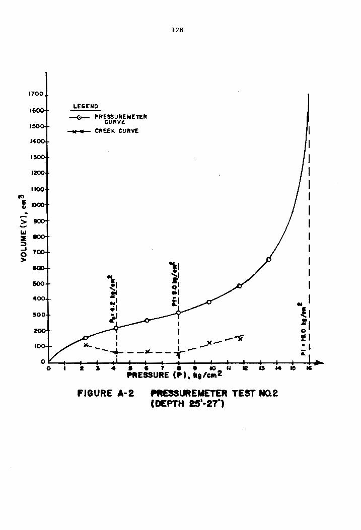
1700

1200

1100

•

LEGEND

--G- PRESSUREMETEIt CURVE

M w CREEK CURVE

128

I

I I ......... -sr ...... I l.,x--

- ........ _..l I .......... -,- ------,

I I I I I I I I I I I I I

.1 !I ., o !!I :'1 ..

J 4 • • 7 • • .Ie) I. PRESSURE C,). Ilg/ .. 2

12 Q M 15 ..

FI8URE A-2 .RESSUREMEIER TEST NO.2 (DEPTH e'-27~)

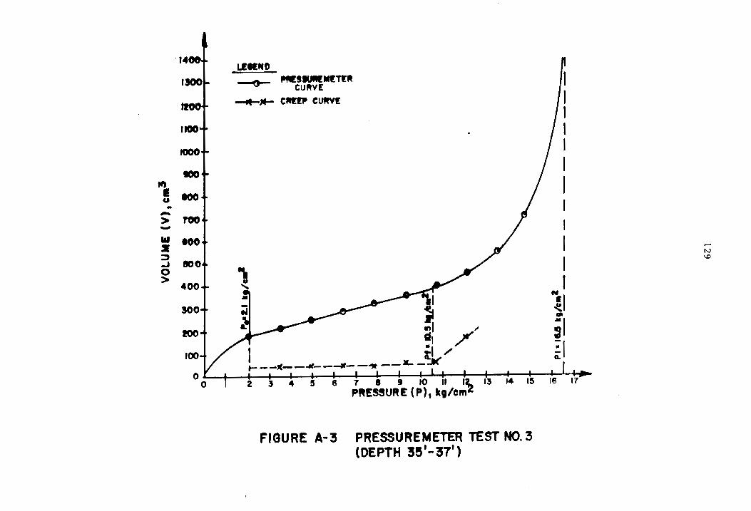
1ft I u • .......

> ....... III 2: ::::)

-' o >

L!.NO ...... fIfII!''''M!T!R

CUftv!:

-tt-.M- CIltRP Cutwt

6 7 • 9 10 II 12.. P"ESSURE (Pl, k,/cmZ

,

FIGURE A-3 PRESSUREMETER TEST NO.3 (DEPTH 3e'-37')

I

I I

N I II il ~I

I--' N \.0

130

--------------1"":J/I'4 .·IZ • hi

~

\c .. 0 \ z

\x In \ "" ~

.... ~,.....

~ LLI-- ........ ",. ~ .' IaJIO .r-t :l:c .. it--Q.. 1aJQ.. - f~ ....

D: => In In ... IIJ

f C iii a= :::> C!) -II...

I i § ~ I § I i ~ 8 0

2 111:» • (A) ~Nn'OA

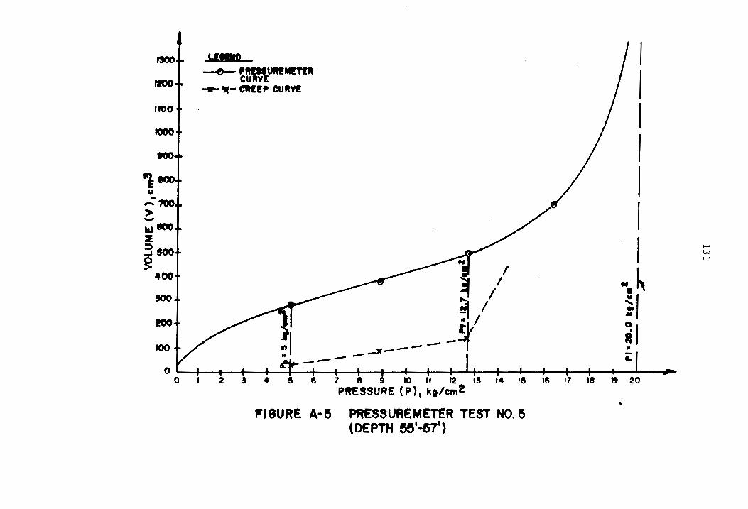
IItJO

1100

tIP) .100, u ..

.... ?aD > -.... ..,100 2 :l g'OC

401

300

100

tOO

LlMIO A- ',,",U ... ttR

CURVE ...... W- CWI!' CUtw!

• ' I

~ / ~/

__ - _-It--- --~

I I I I I I I

"I~ ~I ;, •

0' t' '. If/Ir o 234 !S 8 7 8 9 10 " 12 13 14 I!S 18 11 18 " 20 PRESSURE (P), kltem!

FIGURE A-S PRESSUREMETER TEST NO.5 (DEPTH eel·er')

..... w .....

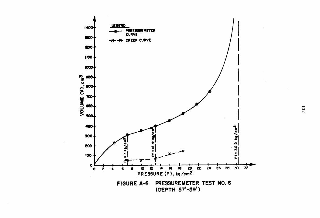
100

100

100

L!1I1IO --0- ,..saJfIIt!M!T!fIt

CUftV!

-.J4-"* CRE!II CUIIIY!

~ ~I

--,r-~-~-'<

I I I

11 ~ ~I a..

or I , I I I , I I. I , • f' I .... o Z 4 I II 10 '2 t4 II .. 20 !O 32

PRESSURE (Pl, ko/em2'

FIGURE A-6 PRESSUREMETER TEST NO.6 (DEPTH 57'-eg')

..... W N

APPENDIX B

Results of CU-Triaxial Tests

Upper Yorktown Formation

133

"

134

I ----.--.- 70,11 I

(~8%f.lS2.Ot PSI :;;..:::-.,--------40 psi

---------------IO~i

0:04 0.05

!-__ -------1'0 ,.,

~f7.7 PSI ",..-_-:.-:~-----_ 40 ,.i -~

" " i1"

/

II) ,.i 0.01 0.0& 0.07

FIGURE 8-1 CU-TRIXIAL TEST CURVES UPPER YORKTOWN FORMATION (DEPTH 37.5'- 40.0')

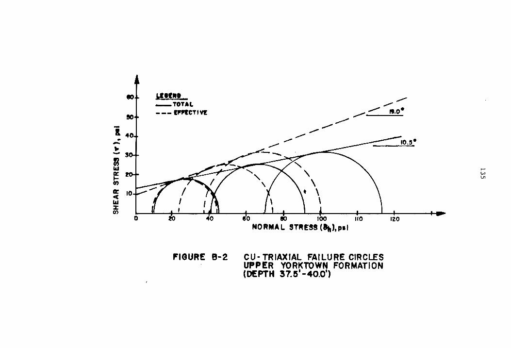
.. .-... ~ 3

~ 1&1 It:

~ a: 10 4( 1&.1 :t: t/)

o

",1'''._ _TOTAL

--- Imerlyt

',GUR£ B-2

~ .""

."",. ,.,.. ~ ".0· ~---~

"", - ~1O.5· ", -

8"0 80 100

NOFtMAL STPtESS <"'),p.,

CU- TRIAXIAL FAILURE CIRCLES UPPER YORKTOWN FORMATION (DEPTH 37.5 1 -40.0')

I-' W \JI

Soil: DolO ror Otvio'oric Modulu. Poromele,. Strattl'1 C1 0010 10'

70 ./. SI,. 1) It'rcl <.) ~ -I. 5 Ire,.. Ltv t I B va ModuhH Po,om (! It 11

0") !OJ -0")1, (OJ . O"J) (0 (Q

IOj- G"Jl Co £0

(OJ' crJ)b Ev 10; '~J!_b

CD ® Q) (~)

10 34.7 24.29 0.0128

40 52.0 36.40 0.0150 ---70 62.5 43.75 0.0093

Po • 14.5 psi

~ I E Po IG,-a)'v" R, Po @ @ ~ @

0.680 1. 66E-2 0.58 212.6 -- - ---_. ----- -----

2.721 1.05E-2 0.55 295.8

4.762 9.75E-3 0.61 566.9

to; crJI

G)

5. 27F.-4

4.10E-4

2.13E-4

8 Po

® --

-

® 32.97

40.94

59.38

5000

2000

1000 Ei/Po

or

~oo a/po

IO",-U))

CD ® ® ~@ 0.0230 6.98E-4 - -

0.0260 . ?~·1?~.::L - ------0.0173 2.91E-4 -

n=0.5 ~ /' \:.J -----_ .. - . ------,.. - -

(U, - U) )ull

Ej Po

JL Po

@-@

0-@ R, (14)

Av.,oQe Rr : 0.58

7..0 I

200

K=70 100

/'

I'"~

V v"'"

./ ./"

/'

lL"

r ~ 0) + ® . @ ,[(3) ~ 0]' Po ~ Po

,---- . 50 OJ 02

.. -,---

0.5 2 () )/Po

FIQJRE JJ-.3 DE'rE~UNATION OF' HYPERBJLIC p~ F'R)'1 CU-TRL1\XIAL 'rES.!'

J (.

(!)

--

-

V

\!r.,..- ...... ....... v

---- I I I 5 10

/'

20 50

I-'

W 0'1

APPENDIX C

Results of CD·Triaxial Tests

Lower Yorktown Formation

137

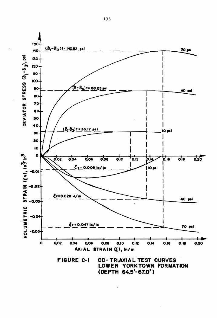
Z -0.01 -C k I-., -0.

U -a:: 1--0. ..... :IE :,)

..J -0.0 o >

138

I I I I I

~~ __ ~ __ -.---,~ __ IO~I

I I

0.04 Q06 0.08

(,.0.047 i./i.

IIO,.i I I

I I

--.--.-------------

I O.tl I I I I I I I

OJI 0:20

40 ,.,

o 0.02 0.04 0.0. 0.01 0.10 0.12 0." 0.11 0.11 0.20

AXIAL STRA IN CE), 'ft/in

FIGURE e-I CD-TRIAXIAL TEST CURVES LOWER YORKTOWN FORMATION (DEPTH 64.5'-67.0')

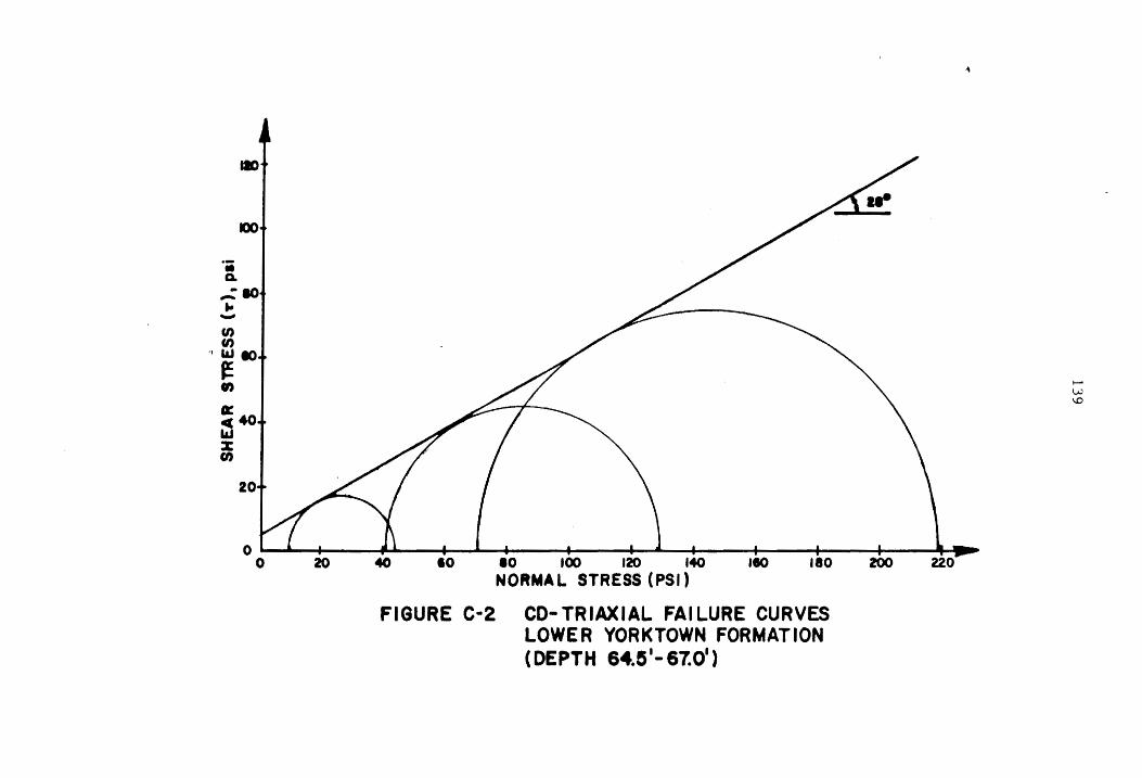
·ii Q.

.,..:'10 .. .......

« 41 40

'" X (I)

20

"

o ' " • II ~ o 20 40 10 10 100 120 140 110 180 200 NORMAL STRESS (PSI)

FIGURE C-2 CD- TRIAXIAL FAI LURE CURVES LOWER YORKTOWN FORMATION (DEPTH 64.e l -67.0·)

220

I--"

W \0

Soil: Doto ror Deviotodc Modulul Po r om ,. era Stratum C2 Ooto tOf

0"")

CD 10

40

70

~ Po

@ 0.680

2.721 -4.762

(0', - O'~ IVII

E, Po

B Po

70 -I. Sire n Leul 9 ~ -I. SIr t n l eYf I Bul' Modulus Parometers

!oj *0")1, (OJ -O"J) (0 Eg

(OJ -0",3'

~ (j) <9 G'> 33.17 23.22 0.030 1.64E-3

88.23 61. 76 0.034 5.59E-4 ------ ---140.82 98.57 0.048 4.87E-4

Po ; 14.S psi

I E, B fa, '0""))1111 R, Po Po

@ e @ ® 2.16E-2 0.71 56.08 41.1

----9.40E-3 0.B3 113.40 129.1

5.62E-3 0.79 139.14 100.7

. - J

R~ : ® I 0> @-G)

CD-@) A.-eroo- R,: 0.78

7,0 I - -0) + ® . @ I [~) ~ (!)] Po

0l Po

(OJ* 0"3'

® 31.51

83.82

133.78

~oo

200

100 Ei!Po

or ~o

B/Po

20

10

:,)-,

(0

<V 0.081

0.091

0.117

01 o 2

(0

(a; oCT))

® 2.57E-J

1. 09E-3 - '-'" ,--8.75E-4

0,5

(OJ -crJ'b Cy

® @ 23.22 0.013

61.76 0.011

98.57 0.023

2 crJ/Po

FIQJHE C-3 OETEr?MINJ\TION OF HYPEPIDLIC P.l\Rn.MF:rERS Fln" CD - TRJJ\XLJ\L TEST

(OJ -a))b

.;\ '=. Gj)

S9S.4

1B71. 5

14E0.1

~ o 20 ~o

.....

.t"­O

APPENDIX D

Results of Soil-Concrete

Interface Tests

141

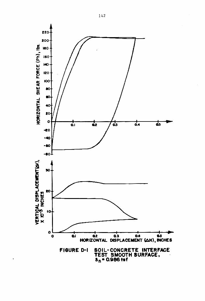
.. ,.... z:: 0.. -...

..J

~ o N

~

142

o~~--~----~----~~----+-----~~~ o Q.I G.2 QI OA o.s HORIZONTAL DlSPLACEMENT~) .INCH£S

FIGURE 0-. SOIL-CONCRETE INTERFACE TEST SMOOTH SURFACE. an • 0.886 taf

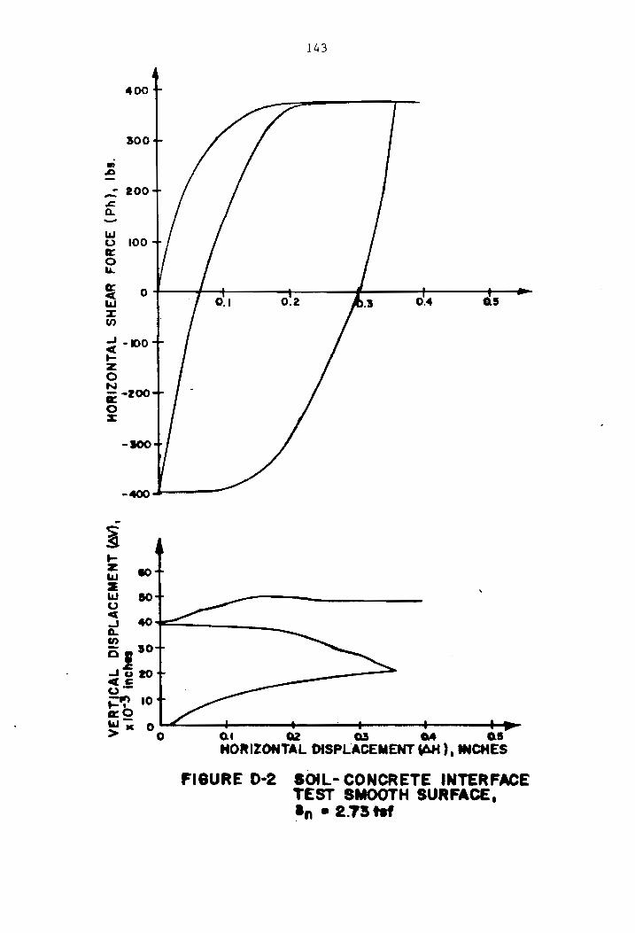
400

100

,.= 100

-LtJ U 100 G: o ....

143

~ o+---~-+------~----~~----~----~~---LtJ 65 % Cf)

...J -100 c: .... z o ~-200 o %

-400~----

0.1 Q2 a:s 64 0.5 HORIZONTAL DISPLACEMENT ~). INCHES

FIGURE 0-2 SOIL- CONCRETE INTERFACE TEST SMOOTH SURFACE, ~n • 2.?5bf

144

-700.-----~----+_----+_----~----~_1~ o OJ Q2 ·03 Oft Q.5

HORIZONTAL DISPLACEMENT ~). INCHES

FIGURE 0-3 SOIL- CONCRETE INTERFACE TEST. SMOOTH SURFACE, aft • 4.481 tlf

145

o~--~~---+----~----+---~~~ o &. QI .. .. • ..1

HORIZONTAL. DISPLACEMENT 16Jt), INOtES

FI.lIItE 0-4 SOIL-CONCRETE INTERFACE TEST, SMOOTH SURFACE, &,.. 4.48' tst

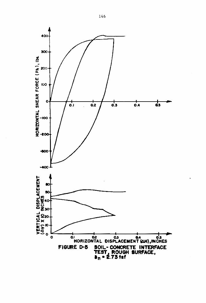
--.r:. 200 Q. -IIJ

~IOO o "-cr; c( I.&J :z: (I)

..J C ~-IOO 2 k i-t

146

QI 02 03 0.4 0.1 HORIZONTAL DISPLACEMENT (AH),tNCHES

FIGlItE o-e IOIL- CONCRETE INTERFACE TEST.t ROUGH SURFACE, an. z.T5t.f

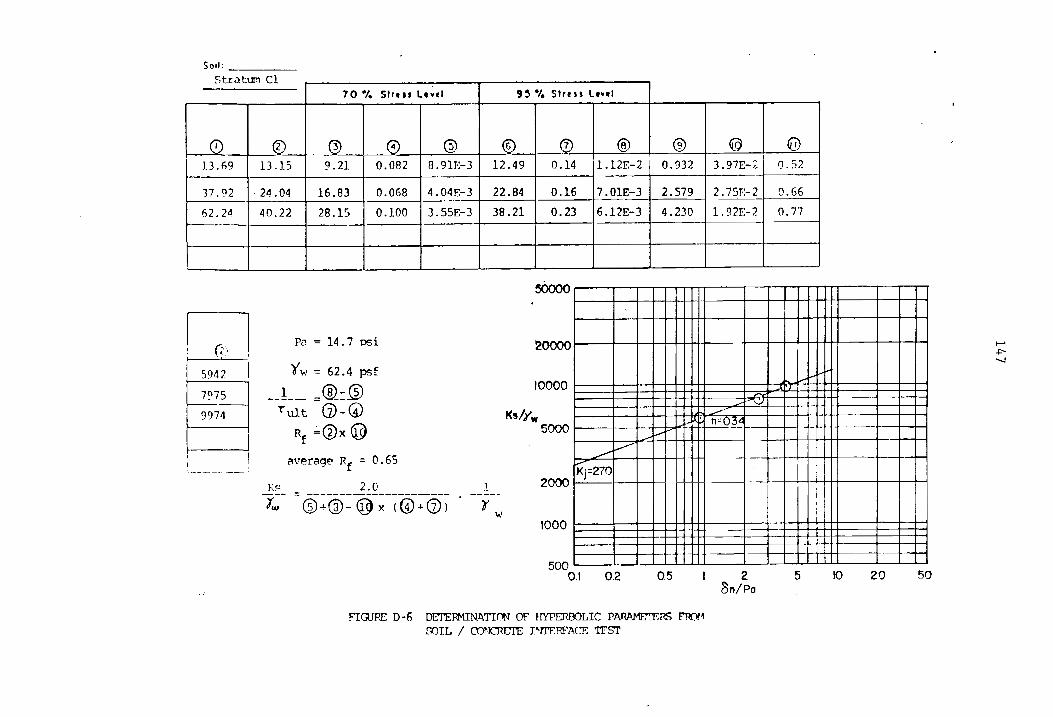
50il: ___ _

Stratum Cl 70 -I. Sire .. L. "" 9 ~ -I. Strf Ii Lty.'

JD CD @ 0 G) © (2) ® ® @ 13. (}9 13.15 9.21 0.082 8.91E-3 12.49 0.14 1.12£-2 0.932 3.97E-2

37.92 ·24.04 16.93 0.068 4.04E-3 22.84 0.16 7.01E-3 2.579 2.75£-2 62.2t1 40.22 28.15 0.100 3.55E-3 38.21 0.23 6.12E-3 4.230 1. 92£-2 ~~

50000

,:l p~ := 14.7 psi 20000

5942 I "I .... , := 62.4 psf

7975

9974 - 1"'V .-or..::.; ..--

1 fa' - f'5l --___ =\2L_~

Tult G)-W 10000

Rf ~@x @ Ks/,( W 5000 ~IJ.. . n=..9:3~

~verage Rf

0.65

K~ 2.0 r:'- = G5="®= @-~-(@ + c2)~

.1

r w

...,.".,..... V V K;=270

2000

1000

500 0.1 0.2

.-1.---' .....

0.5

F'IGURE D"6 DETI:RMIN.n.TI0N OF HYPEROOLIC PA~RS rn:Jt1 ['.oIL / ooncru:::rE PrrEPFACE TFsr

2 8n/Po

(i)

0.52

0.66

0.77

~ ..... ~

5 10 20 50

t--'

+"­-...J

John Christos Daoulas was born on March 19, 1958 in

Wurzburg, Germany to parents that were serving in the U.S.

Army. He was graduated in 1976 from Mount Vernon High

School in Alexandria, Virginia. In June, 1982, he received

a Bachelor of Science Degree in Civil Engineering from

Virginia Polytechnic Institute and State University. Upon

graduation, he was employed as a Staff Engineer by Schnabel

Engineering Associates, P. C. in Richmond, Virginia. He

entered the Virginia Polytechnic Institute Graduate School

in September, 1983 to pursue studies toward a Master of

Science Degree in Civil Engineering. In September, 1984,

Mr. Daoulas returned to Schnabel Engineering where he

currently serves as Senior Project Manager and Branch

Manager for Soil Laboratory Services. Mr. Daoulas was

licensed as a Professional Engineer by the Commonwealth of

Virginia in April, 1987.

148