The Pennsylvania State University

The Graduate School

FINITE ELEMENT ANALYSIS AND A TWO-STAGE DESIGN OPTIMIZATION

PROCEDURE OF MULTIFIELD ORIGAMI-INSPIRED STRUCTURES

A Dissertation in

Mechanical Engineering

by

Wei Zhang

© 2020 Wei Zhang

Submitted in Partial Fulfillment

of the Requirements

for the Degree of

Doctor of Philosophy

May 2020

ii

The dissertation of Wei Zhang was reviewed and approved by the following:

Zoubeida Ounaies

Professor of Mechanical Engineering

Dissertation Co-Adviser

Co-Chair of Committee

Mary I. Frecker

Professor of Mechanical Engineering & Biomedical Engineering

Dissertation Co-Adviser

Co-Chair of Committee

Paris R. von Lockette

Associate Professor of Mechanical Engineering

Timothy W. Simpson

Paul Morrow Professor in Engineering Design and Manufacturing

Francesco Costanzo

Professor of Engineering Science and Mechanics & Mechanical Engineering &

Biomedical Engineering

Karen A. Thole

Professor of Mechanical Engineering

Head of the Department of Mechanical Engineering

iii

ABSTRACT

This dissertation focuses on developing predictive models of the folding performance of

multifield responsive structures and optimizing these structures based on design objectives. In

particular, these origami-inspired structures incorporate smart materials such as electroactive

polymers (EAPs) and magnetoactive elastomers (MAEs), which results in self-folding when one

or more external fields are applied.

Two types of finite element analysis (FEA) models, i.e., continuum modeling and

constitutive modeling, are developed to investigate the actuation performance of self-folding

multifield origami that are actuated using either or both an electroactive polymer, i.e., PVDF-based

terpolymer, and a magneto-active elastomer. In continuum modeling, surface tractions are applied

to simulate the actuation effects resulting from the application of the external fields. The finite

element analysis captures folding performance of electromechanical actuation for notched

configurations and multifield (both magnetic and electric fields) actuation for a bifold structure.

Quantitative comparison using the folding angle as the metric shows that FEA results are

comparable to experiments for the terpolymer actuated single-notch configuration and the

multifield bifold configuration. Geometric parameter studies show that folding angles increase as

the notch length or beam length increases, while beam width does not have a notable effect on

folding.

The constitutive models implemented through the FEA method successfully predict the

coupled responses of the active materials, including folding behavior of the terpolymer-based

actuation of the unimorph and bimorph configurations, the MAE-based actuation of the bimorph,

and simultaneous actuation of the multifield bimorph, where an electric field and a magnetic field

are applied simultaneously. In the modeling the multilayer terpolymer benders, glue layers are

included between the terpolymer layers in the FEA models, and the material properties of the glue

iv

layer are well approximated using a parametric study by comparing to the experiments. In the

simultaneous actuation the multifield bimorph structure, the anticlastic curvature observed in the

experiments is captured in the simulation results, where the curling in the cross-section prevents

the bimorph from further deforming with an increasing external field. The history-dependent

folding performance due to the anticlastic curvature is successfully simulated by the geometrically

nonlinear FEA model.

A computationally efficient two-stage optimization procedure is developed as a systematic

method for the design of multifield origami-inspired self-folding structures. In Stage 1, low-fidelity

models are used within an optimization of the topology of the structure, while in Stage 2, high-

fidelity FEA models are used within an optimization to further improve the best design from Stage

1. The design procedure is first described in a general formulation, applicable to any modeling

methods. Further, to illustrate the optimization procedure, a specific formulation using a rigid body

dynamic model in Stage 1, followed by FEA in Stage 2, is also developed.

To demonstrate the applicability and computational efficiency of the proposed two-stage

optimization procedure, two case studies are investigated, namely, a three-finger soft gripper

actuated using the terpolymer, and an origami-inspired multifield responsive “coffee table”

configuration actuated using the terpolymer and the MAE. In Stage 1, low-fidelity models, such as

analytical models and rigid body dynamic models, are implemented within an optimization of the

topology of the structure, including the placement of the materials, the connectivity between

sections and the amount and orientation of external loads. Distance measures and minimum shape

error are applied as metrics to determine the best design in Stage 1, which then serves as the baseline

design in Stage 2. In Stage 2, the high-fidelity FEA models are used within an optimization to fine-

tune the baseline design. As a result, designs with better performance than the baseline design are

achieved at the end of Stage 2 with computing times of 15 days for the gripper and 9 days for the

v

“coffee table”, which would be over 3 months and 2 mothers for full FEA-based optimizations,

respectively. In the design of the gripper, the best design exhibits a nearly tapered configuration,

where thicker terpolymer and substrate layers are observed in the segments close to the root, while

thinner layers close to the tip, which indicates that the segments close to the root exert greater

influence on the blocked force and conversely the segments close to the tip play a more important

role in enhancing free deflection. In the design of the “coffee table”, wider creases are found

favorable for both electric and magnetic actuations for a higher compliance. Moreover, in the

electric actuation, thinner terpolyemr and substrate are favorable to achieve a higher bending

curvature. To conclude, the applicability and computational efficiency of the two-stage

optimization procedure are demonstrated through the two case studies.

vi

TABLE OF CONTENTS

LIST OF FIGURES ................................................................................................................. viii

LIST OF TABLES ................................................................................................................... xvi

NOMENCLATURE ................................................................................................................ xviii

ACKNOWLEDGEMENTS ..................................................................................................... xx

Chapter 1 Introduction ............................................................................................................. 1

1.1 Motivation .................................................................................................................. 1 1.2 Active Materials for Self-Folding Mechanisms ......................................................... 7 1.3 Modeling Methods for Self-folding Origami ............................................................. 14 1.4 Optimization of Origami Structures and Multi-fidelity Optimization ....................... 19 1.5 Research Objectives and Tasks .................................................................................. 21 1.6 Dissertation Outline ................................................................................................... 23

Chapter 2 Finite Element Analysis of EAP and MAE Actuation for Origami Folding

Using Continuum Modeling ............................................................................................. 26

2.1 Introduction and Motivation ...................................................................................... 26 2.2 Actuation Mechanisms and Simulation Methods ....................................................... 27

2.2.1 Terpolymer Based Actuation .......................................................................... 27 2.2.2 MAE Based Actuation .................................................................................... 30

2.3 FEA Modeling and Verification ................................................................................. 32 2.3.1 Terpolymer-Based Unimorph Bender ............................................................. 32 2.3.2 Single-notch Folding Configuration ................................................................ 36 2.3.3 Parametric Study using FEA ........................................................................... 43 2.3.4 Double-notch Folding Configuration .............................................................. 45 2.3.5 The Bifold Configuration ................................................................................ 48

2.4 Summary .................................................................................................................... 56

Chapter 3 Finite Element Analysis of EAP and MAE Actuation for Origami Folding

Using Constitutive Modeling ........................................................................................... 58

3.1 Introduction and Motivation .................................................................................... 58 3.2 Constitutive Modeling and FEA Implementation ...................................................... 59

3.2.1 Terpolymer-based Actuation ........................................................................... 59 3.2.2 MAE-based Actuation ..................................................................................... 62

3.3 FEA Modeling and Verification ................................................................................. 66 3.3.1 Terpolymer-based Unimorph Bender .............................................................. 66 3.3.2 Multilayer Terpolymer Bender ........................................................................ 70 3.3.3 Single-notch Folding Configuration ................................................................ 72 3.3.4 Double-Notch Finger Configuration ............................................................... 75 3.3.5 The Multifield Bimorph Configuration ........................................................... 76

3.4 Summary .................................................................................................................... 89

vii

Chapter 4 A Two-Stage Optimization Procedure for the Design of Multifield Self-

Folding Structures ............................................................................................................ 91

4.1 Introduction and Motivation ...................................................................................... 91 4.2 A General Formulation of the Two-Stage Optimization Procedure for the Design

of Multifield Self-Folding Structures ....................................................................... 93 4.2.1 Stage 1 ............................................................................................................. 93 4.2.2 Stage 2 ............................................................................................................. 96

4.3 A Particular Formulation of the Two-Stage Optimization Procedure Based on

Rigid Body Dynamic Model .................................................................................... 97 4.3.1 Stage 1 ............................................................................................................. 98 4.3.2 Stage 2 ............................................................................................................. 102

4.4 Summary .................................................................................................................... 104

Chapter 5 Implementation of the Two-Stage Optimization Procedure to Designs of a Soft

Gripper and an Origami-Inspired “Coffee Table” ............................................................ 105

5.1 Introduction ................................................................................................................ 105 5.2 Design of an EAP-Actuated Soft Gripper .................................................................. 108

5.2.1 Introduction and Motivation ............................................................................ 108 5.2.2 PVDF-Based Soft Gripper .............................................................................. 110 5.2.3 The Two-Stage Design Optimization Procedure ............................................. 114 5.2.4 Results ............................................................................................................. 125 5.2.5 Discussion ....................................................................................................... 136

5.3 Design of an Origami-inspired Multifield “Coffee Table” ........................................ 139 5.3.1 Introduction ..................................................................................................... 139 5.3.2 The Two-Stage Design Optimization Procedure ............................................. 140 5.3.3 Results ............................................................................................................. 156 5.3.4 Discussion ....................................................................................................... 166

5.4 Summary .................................................................................................................... 171

Chapter 6 Conclusions and Future Work ................................................................................. 173

6.1 Summary and Conclusions ......................................................................................... 173 6.2 Research Contributions .............................................................................................. 176 6.3 Suggested Future Work .............................................................................................. 178

Bibliography ............................................................................................................................ 181

viii

LIST OF FIGURES

Figure 1-1. The basic shape of the satellite and its array. [34] ................................................ 2

Figure 1-2. Locomotion experiments of crawling robot. (A) and (B) show the large robot

in contraction and expansion status respectively. (C) and (D) show the small robot in

contraction and expansion status respectively [36]. ................................................................. 3

Figure 1-3. Two different designs of the proposed electrode design are shown in the

undeployed ((a) and (d)) and deployed ((b) and (e)) configurations. The design parameters

for each are shown ((c) and(f)).[37] ......................................................................................... 3

Figure 1-4. Ice capsule and deliverer. Ice capsule was colored with food coloring for better

video quality. [38] .................................................................................................................... 4

Figure 1-5. The concept of fluidic origami (a, b). An origami cell was created by connecting

two Miura-Ori sheets along their creases. (c) Three-dimensional topology was created by

integration of different fluid-filled origami cells, where the base unit cell is highlighted. (d)

Shape morphing (folding) can be achieved by controlling the fluidic pressures and

volumes. [41] ........................................................................................................................... 5

Figure 1-6. Bending mechanism of an LIB-based unimorph [43]. .......................................... 5

Figure 1-7. Dielectric elastomer is used as the actuation of a self-folding sheet. The

deformed shape at voltage of 5 KV (b) is compared with the initial shape (a). [31] ............... 8

Figure 1-8. Realization of a cube box and square pyramid using terpolymer unimorph

configuration [50]. ................................................................................................................... 9

Figure 1-9. A bistable origami waterbomb actuated by MAE patches [54]. ........................... 9

Figure 1-10. (a) Schematic of undeformed shape of a multi-segment MAE cantilevered

beam (b) measurement of fold angle after application of magnetic field and (c) image of a

deformed shape. ....................................................................................................................... 10

Figure 1-11. Transformation sequence of the SMA-based origami robot. The robot

undergoes a shape sequence change from the initial resting shape 1 to shape 2 with 90° fold angle on the two joints at the sides, then to shape 3 where all three joints reach a 110° angle forming a tetrahedron [58]. ............................................................................................ 11

Figure 1-12. (a) Stowed configuration and (b) deployed configuration of the SMP

honeycomb. [64] ...................................................................................................................... 11

Figure 1-13. (a) Schematic of the polymer sheet exposed to laser light. (b) Photographs of

the folding of a pre-strained polymer sheet coated with black ink. The sample is

10mm×50mm and is irradiated with a laser beam from left side that covers the sample. [65]

................................................................................................................................................. 13

ix

Figure 1-14. Comparison of actuating mechanisms via prototypes made from PP sheeting.

(a) and (b) Coupled spherical 4-bar Chomper and (c) and (d) four spherical 4-bar coupled

through a 6-bar mechanism. [98] ............................................................................................. 20

Figure 2-1. Compressive pressures are applied through the 3 direction as indicated by red

arrows, and the hollow arrows show the directions of planar expansion in the 1-2 plane. ...... 28

Figure 2-2. The schematic of terpolymer-based unimorph bender. ......................................... 30

Figure 2-3. A pair of horizontal surface loads 𝜏 are applied on the top and bottom surfaces

of MAE patch orienting (a) horizontally and (b) with an angle 𝛼 to the field. ........................ 31

Figure 2-4. Strain in thickness 휀33 and corresponding traction 𝜏33 values. ........................... 33

Figure 2-5. The meshed FEA model of the terpolymer-based unimorph bender. ................... 34

Figure 2-6. Deformed shape comparison of the unimorph bender between experiment (top)

and simulation (bottom) under specified electric fields. .......................................................... 35

Figure 2-7. Comparison of bending curvature between experiment and simulation for the

unimorph bender with electric field ranging from 30 to 70 MV/m. ........................................ 36

Figure 2-8. Schematics of (a) a single-notch unimorph, and (b) the expected folding

deformation in red, and the original position in black. ............................................................ 36

Figure 2-9. The unimorph sample is attached to the glass slide to give the sample a

cantilever constraint. (a) Front view, (b) Side view. Photos were taken by Ahmed. ............... 37

Figure 2-10. The single-notch folding structure is meshed with brick elements. In the notch

region the elements are two times denser than in panel regions along the vertical direction.

(a) The entire meshed structure, and (b) meshed notch region. ............................................... 39

Figure 2-11. Average curvature 𝜅 in the notch and the CPU time as functions of degrees of

freedom of the FEA model. The red dots show the least number of elements that lead to

convergence. ............................................................................................................................ 39

Figure 2-12. Deformed shape comparison between experiment (top) and simulation

(bottom) under specified electric fields and corresponding pressures. .................................... 40

Figure 2-13. Folding angle 𝜃 is defined as the exterior angle between two lines that connect

either end of the sample to the closer edge of the notch. ......................................................... 41

Figure 2-14. Comparison of folding angles between experiment and simulation for the

unimorph single- notch configuration with electric field ranging from 20 to 60 MV/m. ........ 42

Figure 2-15. Folding angles and deformed shapes in notch length study are shown, where

the length of notch changes from 0.5 to 4cm, while the length and width of the beam remain

6cm and 2cm respectively. ....................................................................................................... 44

x

Figure 2-16. Folding angles in beam length study, where the length of the beam changes

from 3cm to 9cm, while the ratio of length-width-notch length remains constant. ................. 45

Figure 2-17. Folding angles in beam width study, where the width of the beam changes

from 1cm to 4cm, while the length and notch length remain 6cm and 2cm respectively. ....... 45

Figure 2-18. The schematic of double-notch folding structure. ............................................... 46

Figure 2-19. Comparison of deformed shapes between the experiments and simulation for

the double-notch configuration. ............................................................................................... 47

Figure 2-20. Comparison of folding angle between experiment and simulation for both

notch 1 and notch 2. ................................................................................................................. 47

Figure 2-21. Design of the bifold. In (a) top view, MAE patches are displayed with the

shown poling directions, leading to a fold about the vertical crease line. In (b) bottom view,

four single-layer terpolymer films are attached to give rise to folding about the horizontal

crease line. ............................................................................................................................... 49

Figure 2-22. Four MAE patches (left) and four single-layer terpolymer actuator strips

(right) are placed on a PDMS substrate to create a multifield bifold. Since the PDMS is

transparent, the sample edges are highlighted in black [112]. ................................................. 49

Figure 2-23. Values of magnetic torque 𝑇 and corresponding surface stresses at different

magnetic fields. ........................................................................................................................ 50

Figure 2-24. Quarter symmetry FEA model of the bifold structure in (a) top view with an

MAE patch and in (b) bottom view with two terpolymer films. The arrows indicate the

symmetry boundary condition applied on that surface. ........................................................... 50

Figure 2-25. The bifold was placed inside of a large, horizontally oriented electromagnet.

Upon application of a magnetic field, the MAE patches rotate to fold the PDMS substrate

as they attempt to align with the applied field [112]. ............................................................... 51

Figure 2-26. The simulated image of the actuated quarter of bifold under field strength

0.1195 T. according to the symmetry of bifold geometry, 𝜃 indicates half of the folding

angle. ........................................................................................................................................ 52

Figure 2-27. Comparison of folding angle between simulation and experiment for MAE

actuation of the bifold. ............................................................................................................. 52

Figure 2-28. The bifold sample is hung using tweezers and folds in the horizontal plane for

terpolymer actuation. ............................................................................................................... 53

Figure 2-29. Deformed shapes of the bifold actuated using electric field of (a) 0 MV/m, (b)

40MV/m and (c) 70 MV/m. ..................................................................................................... 54

xi

Figure 2-30. Overall mesh assignment viewed from the side of terpolymer films (a) and

exaggerated root region (b). The mesh density is much higher in root region than in other

parts in order to reduce influence of stress concentration. ....................................................... 54

Figure 2-31. The deformed shape in simulation under electric field of 70 MV/m for

terpolymer actuation. According to the symmetry of bifold geometry, 𝜃 is half of the

folding angle. ........................................................................................................................... 55

Figure 2-32. The von Mises stress of terpolymer strips and PDMS matrix are shown. .......... 55

Figure 2-33. Comparison of folding angle between experiment and simulation for

terpolymer actuation. ............................................................................................................... 56

Figure 3-1. Rotation of a shell element can be interpreted using the displacement in unit

normal vector. .......................................................................................................................... 64

Figure 3-2. A schematic of the shell model of the unimorph bender is shown as (a), where

the offset of the midsurfaces account for the thickness. The meshed FEA model for the

bender is shown as (b). ............................................................................................................. 67

Figure 3-3. The measured longitudinal strain 휀33 and the calculated coupling coefficient

𝑀33are shown with electric field ranging from 0 to 70 MV/m. .............................................. 67

Figure 3-4. The deformed shapes of the unimorph bender are compared between

experiments and FEA. .............................................................................................................. 69

Figure 3-5. The bending curvatures of the unimorph bender are measured for experiments

and FEA with 𝑘 varying from 0.5 to 0.9. ................................................................................. 69

Figure 3-6. The schematic of a unimorph bender actuated using double-layer terpolymer. .... 70

Figure 3-7. FEA results are compared with experiments in bending curvatures of 2-layer,

4-layer and 6-layer terpolymer-actuated benders. .................................................................... 71

Figure 3-8. The sensitivity study of the glue layer to the bending curvature. .......................... 72

Figure 3-9. Two issues are observed in the original FEA model (top); so, modifications are

made in the later model (bottom). ............................................................................................ 73

Figure 3-10. Deformed shapes of experimental samples and FEA results are shown for

electric field ranging from 0 to 60 MV/m. ............................................................................... 74

Figure 3-11. Folding angle comparison between experiments and FEA results for the

single-notch configuration. ...................................................................................................... 75

Figure 3-12. The terpolymer-based finger configuration is developed to imitate motion of

a finger, a schematic shown in (a) and a real sample shown in (b). [118] ............................... 75

xii

Figure 3-13. The deformed shapes of the finger configuration from FEA results are

compared with experiments. .................................................................................................... 76

Figure 3-14. Schematic and corresponding fabricated sample of the multifield responsive

bimorph configuration. The photo was taken by Sarah Masters. ............................................. 77

Figure 3-15. Meshed model and zoomed top gap are shown for the bimorph configuration.

................................................................................................................................................. 78

Figure 3-16. Deformed shapes of experiments and FEA results for the terpolymer-based

actuation of the bimorph configuration. ................................................................................... 78

Figure 3-17. Folding angle comparison between experiment and FEA results for

terpolymer-based actuation of the bimorph. ............................................................................ 80

Figure 3-18. The bimorph is placed in an external magnetic field in positive z-direction.

The two MAE patches generate magnetic torques 𝑻 that rotate the top patch rightward and

bottom patch leftward. Gravity is in negative z-direction. ....................................................... 81

Figure 3-19. Deformed shape comparison between experiments and FEA results for MAE-

based actuation of the bimorph configuration. ......................................................................... 81

Figure 3-20. Comparison of folding angle between experiments and simulation results for

MAE-based actuation of the bimorph configuration. .............................................................. 82

Figure 3-21. Deformed shape comparison between experiments and FEA results for MAE-

based actuation of the bimorph configuration at fixed 𝜇0𝐻0 = 38𝑚𝑇 and increasing

electric field strengths. ............................................................................................................. 83

Figure 3-22. Tip displacement in x-direction of FEA results and experiments for

simultaneous actuation of the bimorph. ................................................................................... 84

Figure 3-23. Tip displacement in z-direction of FEA results and experiments for

simultaneous actuation of the bimorph. ................................................................................... 85

Figure 3-24. Anticlastic curvature occurs in both (a) experiment and (b) FEA in the

simultaneous actuation of the bimorph when E=60MV/m and lead to a straight shape rather

than folded. .............................................................................................................................. 86

Figure 3-25. The deformed shapes of the bimorph under different sets of simultaneous

actuation. It shows that the loading history has an effect on the deformation due to

appearance of the anticlastic curvature. ................................................................................... 88

Figure 3-26. The simulation results of the bimorph under different sets of simultaneously

applied electric (E) and magnetic (H) fields. It demonstrates that the FEA model is able to

reflect the effect of loading history which also appears in experiments. ................................. 88

Figure 4-1. A general formulation of the two-stage optimization procedure. .......................... 94

xiii

Figure 4-2. Example formulation of the two-stage optimization procedure where rigid body

dynamic models are used in Stage 1. ....................................................................................... 98

Figure 4-3. A crease could be modeled as a revolute joint with a torsional spring using the

small length flexural pivot (SLFP) model. Gray indicates rigid panels and white illustrates

the compliant crease material.[112] ......................................................................................... 99

Figure 5-1. (a) Schematic of the “finger” configuration. (b) Photo of a “finger” sample at

rest and (c) folded upon application of electric field. .............................................................. 111

Figure 5-2. The assembled gripping base. ............................................................................... 112

Figure 5-3. Grasping experiments for several target objects including (a) a 60 mm pom-

pom ball, (b) a paper cylinder and (c) an inflated latex glove. ................................................ 113

Figure 5-4. The flowchart of the two-stage optimization procedure for gripper design. ......... 115

Figure 5-5. Schematic of the five-segment actuator. ............................................................... 115

Figure 5-6. The schematics of (a) the undeformed unimorph, (b) the deformed unimorph

with bending curvature 𝛋 and (c) two segments with their angular deflections. ..................... 117

Figure 5-7. The schematics of (a) the equivalent bending moment and blocked force acting

on an actuator with 𝐧 segments and (b) the inner moment on the 𝐢th segment. ...................... 120

Figure 5-8. The trapezoid shape of surface of the 𝐢th segment with edge slope 𝑺𝒍𝒐𝒑𝒆𝒊. The

area of the surface and accordingly the volume of the materials remain the same from Stage

1 to Stage 2. ............................................................................................................................. 122

Figure 5-9. Roller boundary condition is assigned at the bottom edge of the unimorph

bender to compute the blocked force. ...................................................................................... 123

Figure 5-10. Blocked force comparison between FEA and experiments for the unimorph

bender. ...................................................................................................................................... 124

Figure 5-11. The meshed FEA model with trapezoid segment surfaces where 𝑺𝒍𝒐𝒑𝒆𝒊 =𝟎. 𝟏𝟐. A symmetric boundary condition is applied along the center line considering the

symmetric geometry of the actuator. ....................................................................................... 125

Figure 5-12. The performance space of the standard unimorph and the final generation from

Stage 1. The position of the best design in Stage 1 is determined by the minimum value of

distance measure. ..................................................................................................................... 128

Figure 5-13. Schematics of (a) the best design from Stage 1, showing a nearly tapered

configuration along the length, and (b) a standard unimorph. The thicknesses are

exaggerated compared to lengths. ............................................................................................ 128

xiv

Figure 5-14. The positions of the 15 selected designs in (a) performance space of the

parametric design when 𝐸 = 40 𝑀𝑉/𝑚 and (b) when 𝐸 = 1 𝑀𝑉/𝑚 . .................................. 130

Figure 5-15. (a) The performance space of the best design in Stage 1, the initial generation

and pareto front of the 51st generation in Stage 2. (b) a zoomed plot of the designs in the

51st generation. ........................................................................................................................ 132

Figure 5-16. The trend of spreadchange value in the last 11 generations where the algorithm

tends to converge. .................................................................................................................... 133

Figure 5-17. Schematic of the best design generated from Stage 2, where the thicknesses

are exaggerated compared to lengths. ...................................................................................... 133

Figure 5-18. The simulated deformed shapes of the standard unimorph and best designs in

Stage 1 and in Stage 2 under free deflection and blocked conditions. ..................................... 135

Figure 5-19. The trade-off between model accuracy and computational efficiency is

presented by comparing the analytical model and FEA model. ............................................... 138

Figure 5-20. A real origami-inspired coffee table [155]. ......................................................... 140

Figure 5-21. Schematics of the target shapes for the “coffee table” upon application of

magnetic field (a), electric field (b)and both fields simultaneously(c). ................................... 141

Figure 5-22. The flowchart of Stage 1 for the “coffee table” design. ...................................... 141

Figure 5-23. A crease can be folded as either a mountain fold (in red) or a valley fold (in

blue) in the software “origami pattern designer” [18]. ............................................................ 142

Figure 5-24. (a) The crease pattern of the “coffee table” designed in the software “origami

pattern designer”, where the red creases represent mountain creases, while the blue ones

represent valley creases. (b) The deformed shape with corresponding folding angles. ........... 143

Figure 5-25. Schematic of the rigid body dynamic model of the “coffee table”. .................... 143

Figure 5-26. The positions of the magnetic and electric creases. ............................................ 145

Figure 5-27. Simulation result of a deformed rigid body model, where the dots represent

the nodes used in shape error calculation................................................................................. 146

Figure 5-28. The flowchart of Stage 2 for the design of “coffee table”. .................................. 149

Figure 5-29. The meshed FEA model for (a) the entire geometry and (b) the half geometry.

................................................................................................................................................. 149

Figure 5-30. (a)The half-geometry FEA model for magnetic actuation and (b) the front

view of the magnetic panels and creases. ................................................................................ 150

xv

Figure 5-31. Schematics to illustrate (a) the directions of remanent magnetization 𝑴 and

normal vector 𝒏 in the initial configuration and (b) the deformed magnetic panel. ................ 151

Figure 5-32. An example to illustrate the deformed shapes when the two-step method is

applied in FEA. ........................................................................................................................ 152

Figure 5-33. Meshed FEA model for terpolymer actuation and the nodes to calculate shape

error 𝝍. ..................................................................................................................................... 154

Figure 5-34. Schematics of (a) top view and (b) front view of the electric crease shown as

the dashed part in the model for terpolymer actuation. ............................................................ 155

Figure 5-35. The performance space of the 23rd generation with the best design circled. ...... 157

Figure 5-36. (a) The simulated deformed shape of the best design in Stage 1, with the angels

measured between the horizontal line and the magnetic panels in (b) and the electric angles

in (c). ........................................................................................................................................ 158

Figure 5-37. The performance space of the 2nd generation. .................................................... 161

Figure 5-38. The deformed shape of (a) a half-geometry model and (b) a full-geometry

model of the best design in Stage 2 of magnetic actuation. ..................................................... 162

Figure 5-39. The performance space of the 13th generation of terpolymer actuation in Stage

2, with the baseline design shown and best design circled. ..................................................... 165

Figure 5-40. The deformed shape of (a) a corner model and (b) a full-geometry model of

the best design in Stage 2 of electric actuation. ....................................................................... 165

Figure 5-41. The trade-off between model accuracy and computational efficiency is

presented by comparing the rigid body model and FEA model. .............................................. 169

xvi

LIST OF TABLES

Table 1-1. Comparison of active materials used to realize self-folding of origami-inspired

devices. [32] ............................................................................................................................. 14

Table 1-2. Comparison of analytical, kinematic, dynamic and finite element modeling of

active structures. [79] ............................................................................................................... 15

Table 1-3.Correlation of dissertation chapters with tasks addressed in each chapter. ............. 25

Table 2-1. Modeling parameters of the unimorph bender configuration. ................................ 33

Table 2-2. Modeling parameters for single-notch folding configuration. ................................ 37

Table 2-3. Material properties and dimensions of MAE patches. ............................................ 50

Table 3-1. Geometries and material properties for the bimorph configuration. ....................... 78

Table 5-1. Dimensions and material properties for the “finger” configuration. ...................... 112

Table 5-2. The values of the design variables for the best design in Stage 1. ......................... 129

Table 5-3. Performance comparison between the standard unimorph and the best design in

Stage 1. ..................................................................................................................................... 129

Table 5-4. The values of the design variables for the best design in Stage 2 .......................... 134

Table 5-5. Performance comparison among the standard unimorph, the best design in stage

one and the best design in Stage 2 based on the FEA model when 𝑬 = 𝟒𝟎 𝑴𝑽/𝒎. .............. 134

Table 5-6. The dimensions, material properties and corresponding torsional spring

constants in Stage 1. ................................................................................................................. 145

Table 5-7. The torques and deformed angles of the best design in Stage 1. ............................ 159

Table 5-8. Values of the MAE thicknesses in the best design in Stage 1 and the ranges of

the design variables in Stage 2. ................................................................................................ 160

Table 5-9. The parameters of the best design in Stage 2 of magnetic actuation. ..................... 162

Table 5-10. A comparison of the objectives and distance measure between the best,

baseline and two other designs in Stage 2 of electric actuation. .............................................. 162

Table 5-11. Values of the MAE thicknesses in the best design in Stage 1 and the ranges of

the design ................................................................................................................................. 164

Table 5-12. The parameters of the best design in Stage 2 of electric actuation. ...................... 165

xvii

Table 5-13. A comparison of the objectives and distance measure between the best and

baseline designs in Stage 2 of electric actuation. ..................................................................... 165

xviii

NOMENCLATURE

Symbol Description

𝒂 ∗ Displacement vector of a unit normal vector

𝐴 Area

𝑎𝑥, 𝑎𝑦, 𝑎𝑧

𝑛𝑥

𝑛𝑥

Components of displacement of a unit normal vector

𝒃 Body force

𝑐 Weight in distance measure

𝐶 Total number of the creases

d Distance

𝐸, 𝐸𝑖 Electric field

𝐹𝑏 Blocked force

𝒈 Gravitational acceleration

ℎ Type of external field

𝑯 Magnetic field

𝑖, 𝑗, 𝑘 Index

𝑘13 Ratio of the transverse strain to the longitudinal strain

𝑘𝑜 Number of design objectives

𝐾 Spring constant of a revolute joint

𝑙 Material length

𝑚 Torque generated by a unit volume of the active material

𝑴 Remanent magnetization per unit volume

𝑀𝑖𝑗, 𝑀𝑖𝑗𝑘𝑙 Electro-mechanical coupling coefficient

𝑀𝑒𝑞 , 𝑀𝑖𝑛𝑡 Equivalent and internal bending moment

𝐧 Unit normal vector

𝑛𝑥, 𝑛𝑦, 𝑛𝑧

𝑛𝑥

𝑛𝑥

Components of unit normal vector

𝑁 Total number of the nodes

𝑜𝑏𝑗 Design objective value

𝑜𝑏𝑗𝑙𝑜𝑤 Design objectives for the low-fidelity models

𝑜𝑏𝑗𝐹𝐸𝐴 Design objectives for the FEA models

𝑝 Power in distance measure

𝑃 Total number of the panels

𝑹 Rotation matrix

xix

𝑆𝑖𝑗𝑘𝑙 Material compliance

𝑡 Material thickness

𝑻 Magnetic torque

𝑈 Distance measure score

𝒗 Velocity

𝑉 Material volume

𝑣𝑎𝑟 Design variables

𝑣𝑎𝑟1 Design variables in Stage 1

𝑣𝑎𝑟2 Design variables in Stage 2

𝑣𝑎𝑟𝑒𝑓𝑓 Effective design variables

𝑣𝑎𝑟𝑖𝑛 Initial design variable values

𝑣𝑎𝑟𝑢𝑝 Updated design variable values

𝑤 Material width

𝑥, 𝑦, 𝑧 Cartesian coordinate system

𝑥0, 𝑦0, 𝑧0 Cartesian coordinates of the target shape

𝑌, 𝑌𝑖𝑗𝑘𝑙 Elastic modulus

𝛼, 𝛽 Rotation angle

𝛼𝑙 The lower factor

𝛼𝑢 The upper factor

𝛿 Tip displacement

Δ𝑓𝑟𝑒𝑒 Free deflection

𝜓 Shape error

𝜺 Strain

𝝈 Stress

𝜆, 𝜇

𝜇

Elastic parameters

𝜆𝑛 Dual factor

𝜐 Poisson’s ratio

𝜌 Material density

𝜃 Folding angle

𝜅 Bending curvature

𝜏 Surface traction

Ω Penalty term

*The bolded symbols represent the vectors, matrices or tensors, while the correspoding unbolded symbols represent their

magnitudes.

xx

ACKNOWLEDGEMENTS

I would first like to thank my dissertation advisors, Drs. Zoubeida Ounaies and Mary

Frecker, without whom I could not have become a qualified researcher and achieved this much in

the research field. I sincerely appreciate the time, efforts and most importantly, patience they have

put in supervising me during weekly meetings and editing all my research writings. Their research

insights and integrity have influenced me much and will be my life-long treasures.

I am grateful for the supporting committee, which contains Dr. von Lockette, Dr. Simpson

and Dr. Costanzo besides my advisors. Whenever I was in trouble with either computational

modeling or material physics, and asking for their help, they always kindly spared their time with

me and offered valuable thoughts and suggestions. I appreciate the support from my committee

members sincerely.

I always feel lucky to work with the collaborative, kind and caring labmates from the

EMCLab led by Dr. Ounaies, EDOG lab jointly led by Dr. Frecker and Dr. Simpson, and the EFRI

team which contained even more professors and students. I am grateful for my labmates Ahmed,

Jon Hong, Sarah Masters and Corey Breznak, who have put great efforts to conduct the experiments

which are extremely important to validate my models and provide physics insights. I appreciate the

help from Dr. Bowen, Dr. Calogero, Brad Hanks, Jivtesh Khurana and Cody Gonzalez who helped

me a lot solve the problems in my software programs and optimization algorithms.

I am grateful for the generous funding of our work by the National Science Foundation

and the Air Force Office of Scientific Research (grant number 1240459). Without this funding, my

work would not be possible.

I am so thankful for the unconditional love and support from my family. My wife Bing

Bong has been my closest friend and strongest mental reliance. We have learned so much from

each other during our Ph.D. careers and conquered many obstacles together through this

xxi

challenging process. My parents are so wonderful that their love provides to me the ultimate

courage to try and to grow. I will respond to your love with my love and make you proud.

1

Chapter 1

Introduction

1.1 Motivation

This dissertation focuses on developing predictive models and optimizing the folding

performance of origami-inspired multifield responsive structures. In recent years, the promise of

origami-inspired folding and assembly of materials and structures have broadly inspired researchers

and engineers. Origami is an ancient Japanese art which involves folding flat paper into various

three-dimensional shapes [1]. Origami continues to draw interest from artists and mathematicians

on the design of complex shapes and path planning analysis. Montroll [2] provided step-by-step

instructions on over 700 diagrams for different origami configurations. The concept of origami has

also inspired engineering design [3–12] due to its simple assembly process (folding), the ability to

reversibly fold and unfold to desired shapes and the corresponding potential for lower cost and

weight compared to traditional mechanical designs. Hull developed mathematical expressions and

theorems for folding flat sheets into either 2-D configurations called flat folding, or 3-D

configurations called non-flat folding [4,13,14], and those theorems have been successfully applied

to the design of reprogrammable structures [15]. Balkcom and Mason [16] introduced the first

origami-folding robot and analyzed the classes of folding it could realize. Later on, kinematic

analysis of folding joints and compliant mechanisms has been conducted by numerous researchers,

such as Bowen [17], Xi [18] and Greenberg [19].

Origami-inspired engineering has given rise to novel applications in many different fields

such as solar arrays [20] [21], paper batteries [22], robotics [23,24], inkjet printing [25] and

biomedical devices [26]. Multiple actuation mechanisms are used to actuate origami design

2

including light absorption [27,28], shape memory alloys [29], electroactive [30,31] and

magnetoactive actuation systems [32,33]. Several applications of origami engineering are

summarized next.

In solar arrays, Holland et al. [34] proposed an origami-style deployment approach which

enhanced the efficiency of transmission by largely increasing collection and transmission surface

areas while keeping comparable mass and volume compared to other designs. The design pattern

is shown in Figure 1-1.

Figure 1-1. The basic shape of the satellite and its array. [34]

Other applications are found in robotics. Cheng et al. [35] created active bi-directional

motion in robot joints which were actuated using shape memory alloys for meso-scale minimally

invasive neurosurgical applications. Pagano et al. [36] proposed the design of a bio-inspired

origami crawling robot, where the Kreslin-like origami towers were used as the locomotion

mechanism for the first time. Forward locomotion and steering of the mechanism were realized by

the actuation of DC motors, which expanded and contracted the origami patterns, as shown in

Figure 1-2.

3

Figure 1-2. Locomotion experiments of crawling robot. (A) and (B) show the large robot in contraction and

expansion status respectively. (C) and (D) show the small robot in contraction and expansion status

respectively [36].

Hanks et al. [37] presented a design and optimization procedure of an origami-inspired

deployable compliant endoscopic radiofrequency ablation probe, which intentionally deploys the

tines to match the ablation zone to the destructed tissues. The schematic of the undeployed and

deployed states and the design parameters are shown in Figure 1-3.

Figure 1-3. Two different designs of the proposed electrode design are shown in the undeployed ((a) and

(d)) and deployed ((b) and (e)) configurations. The design parameters for each are shown ((c) and(f)).[37]

4

Another example is the ingestible, controllable and degradable origami robot for patching

stomach wounds developed by Miyashita et al. [38]. The robot was composed of biocompatible

and biodegradable materials and could be folded and embedded in an ice capsule for delivery into

stomach. Magnetic field would be applied to remotely control the robot to carry out the underwater

maneuvers after fulfillment of the task. The capsule and deployed state are shown in Figure 1-4.

Figure 1-4. Ice capsule and deliverer. Ice capsule was colored with food coloring for better video quality.

[38]

An emerging type of origami engineering called fluidic origami was inspired by the idea

that architectured material could be achieved by intentionally stacking and connecting multiple

origami sheets together [39]. Relationship between folding and constituent sheet deformations were

investigated to achieve desired properties and functions. This pressurized stacked-origami concept

has been shown to exhibit shape transformation, stiffness control, and recoverable collapse [40,41].

A schematic to illustrate the concept of fluidic origami is shown in Figure 1-5.

5

Figure 1-5. The concept of fluidic origami (a, b). An origami cell was created by connecting two Miura-Ori

sheets along their creases. (c) Three-dimensional topology was created by integration of different fluid-

filled origami cells, where the base unit cell is highlighted. (d) Shape morphing (folding) can be achieved

by controlling the fluidic pressures and volumes. [41]

The idea of origami folding has also been applied in battery to achieve large and

controllable deformations. Gonzalez et al. [42,43] developed analytical models and finite element

models to investigate the deformation and blocked force, which is the actuation force when the tip

of the structure is held constant, of the segmented unimorph based on lithium-ion batteries (LIB).

Bending performance is achieved due to the volumetric expansion of the lithiation of silicon, which

could be over 300% when the battery is fully charged, as shown in Figure 1-6.

Figure 1-6. Bending mechanism of an LIB-based unimorph [43].

6

In general, origami-inspired structures can be classified into two categories based on their

actuation mechanisms. The first category is manual-folding structures, where the folding of the

structures is actuated directly using external forces, such as hands or motors. The second category

is self-folding structures, where the active materials are embedded in the structure, realizing folding

in response to external stimuli. This dissertation focuses on the latter, i.e., self-folding structures,

for their capacity to achieve complex deformations with high automation, which enables them to

function in environments where physical access is not possible or light weight is preferable or

necessary.

In the design of self-folding structures, the designers need to consider following questions:

• What is the final target shape that needs to be achieved under actuation?

• What folds are needed and where should they be placed in order to achieve the target shape?

• Which types of active materials are capable of actuating the structure? Is one single type

of active material sufficient, or are multiple fields needed?

• How much displacement and actuation force will the structure require when in use, for

example to grab an object or deploy under load? And generally, how does one deal with

the tradeoff between conflicting design objectives?

For a single origami design, these questions are not difficult to answer through trial-and-

error experimentation. However, there are several major challenges in experimentation, such as the

time and cost to fabricate the active and inactive materials, the need for multiple samples to increase

reliability and repeatability of results, and the inconvenience of the trial-and-error iterations due to

not knowing optimal values for the design parameters. Because of these challenges, there is a

necessity to model the origami structures to predict their performance. After validating the models

using experiments, one can use the models to predict the deformed shapes of the structure actuated

using specified field strengths, to investigate the sensitivity of actuation performance to the design

7

parameters, and to optimize these parameters based on design objectives such as to minimize the

amount of active materials needed or to minimize the shape error between actual and target shapes.

In the remainder of this chapter, a review on active materials for self-folding mechanisms,

modeling methods including kinematic, analytical, rigid-body dynamics and finite element method,

and optimization methods such as topology optimization, genetic algorithm (GA), multi-fidelity

optimization and reduced basis method, are summarized in Sections 1.2-1.4, respectively. The

research objectives and tasks are described in Section 1.5, and the outline of this dissertation is

presented in Section 1.6.

1.2 Active Materials for Self-Folding Mechanisms

According to Liu et al. [44], “self-folding is a deterministic assembly process that causes a

predefined 2D template to fold into a desired 3D structure with high fidelity”. Many types of active

materials have been investigated and applied to realize origami-inspired self-folding structures. In

the following discussion, a selection of the most commonly used active materials in the self-folding

literature are briefly described, and examples of their use are listed.

Dielectric elastomers (DE) consist of an elastomer sandwiched between two compliant

electrodes [45]. Upon application of a high voltage across the electrodes, the elastomer compresses

in thickness and expands in plane. When a DE is attached to an inactive substrate, the planar motion

is constrained, resulting in bending as shown in Figure 1-7; localized bending becomes folding in

origami structures [31]. Ahmed et al. [31] demonstrated use of a DE bending actuator, fabricated

using a thin 3M VHB double-sided tape and conductive rubber or carbon grease as electrodes. The

thickness of a single layer of commercially-available DE typically ranges from 50 μm to 2000 μm

[46], and several electroded layers can be stacked up to improve actuation performance [47].

8

(a) (b)

Figure 1-7. Dielectric elastomer is used as the actuation of a self-folding sheet. The deformed shape at

voltage of 5 KV (b) is compared with the initial shape (a). [31]

Another electroactive polymer (EAP) that has been used to actuate origami structures is

P(VDF-TrFE-CTFE) terpolymer; this terpolymer is a relaxor ferroelectric owing to the presence of

the chlorotrifluoroethylene (CTFE) monomer, which acts as a defect into the ferroelectric P(VDF-

TrFE) copolymer. This terpolymer has many advantageous attributes as actuator, such as a high

electrostrictive strain of up to 7%, a relatively high dielectric constant of 50, and a moderate

breakdown electric field of 400MV/m [48,49]. Similar to DE, when electric field is applied, the

terpolymer layer will contract in thickness direction and expand in-plane. If we attach an inactive

substrate to the terpolymer, then the in-plane expansion will be constrained, causing bending

[30,50,51]. Active folding can be achieved by introducing non-uniform thickness along the length

direction of the sample, whereas localized bending occurs in the thinner region, i.e., notch region

[50]. An example of a terpolymer-actuated box is shown in Figure 1-8.

9

Figure 1-8. Realization of a cube box and square pyramid using terpolymer unimorph configuration [50].

Magnetoactive elastomers (MAEs) are another class of smart materials; they are fabricated

by embedding hard-magnetic particles such as barium hexaferrite into an elastomer matrix. When

MAEs are placed in an external magnetic field, the magnetized particles rotate to align with the

external field, thus generating magnetic torques [52–54]. The two stable states of a bi-stable paper

origami waterbomb base actuated by MAE patches are shown in Figure 1-9. By distributing non-

uniform thickness through the structures, the magnetic torques will cause localized bending,

namely, folding, and deploy the structures to target shapes. A MAE-based multi-segment

cantilevered beam was developed in [53], as shown in Figure 1-10, where folding appeared in the

thinner regions with no MAE patches after the magnetic field was applied.

Figure 1-9. A bistable origami waterbomb actuated by MAE patches [54].

10

(a) (b) (c)

Figure 1-10. (a) Schematic of undeformed shape of a multi-segment MAE cantilevered beam (b)

measurement of fold angle after application of magnetic field and (c) image of a deformed shape.

Shape memory materials, such as shape memory alloys (SMAs) and shape memory

polymers (SMPs), are a class of smart materials that can recover their original shape after large

deformation in the presence of temperature change. Shape memory alloy, commonly made of nickel

and titanium alloy (Nitinol), has received wide interest from both research and industry due to its

ability to deform with high force output [55–57]. Zhakypov et al. [58] introduced a novel low-

profile torsional SMA actuator designed to actuate self-folding origami. They conducted

experiments to characterize the performance of the actuator under different conditions including

with load, without load, and in blocked conditions, and they developed and validated a thermo-

mechanical model for the SMA actuator. The transformation sequence of the SMA-actuated robot

is shown in Figure 1-10.

11

Figure 1-11. Transformation sequence of the SMA-based origami robot. The robot undergoes

a shape sequence change from the initial resting shape 1 to shape 2 with 90° fold angle on the two joints at

the sides, then to shape 3 where all three joints reach a 110° angle forming a tetrahedron [58].

SMPs are polymers that possess the ability [59] to transform between several

configurations in response to an external stimulus such as heat, electricity, magnetism, moisture

and light . Compared to SMAs, SMPs can achieve large strains (up to 800%) with relatively small

stresses (1–3 MPa), and exhibit better manufacturability and customizability [60]. SMPs have been

widely used for applications related to shape morphing [59,61–63].

Neville et al. [64] investigated a SMP honeycomb with tunable and shape morphing

mechanical characteristics, which was designed and manufactured using kirigami techniques, a

variation of origami that includes cutting of the base materials. The stowed and deployed

configurations of a SMP honeycomb are shown in Figure 1-11.

Figure 1-12. (a) Stowed configuration and (b) deployed configuration of the SMP honeycomb. [64]

12

There is a type of SMP that the shape memory effect is triggered by light absorption which

results in heating, referred to as light-responsive materials. Light shows several superior properties

as an external stimulus to induce folding compared to other mechanisms. For example, light can

uniquely be applied to the target structure remotely with little loss, whereas the wavelength,

intensity and spatial distribution of the light would be conveniently manipulated [65]. One approach

to achieve folding is to apply a uniform irradiation, where there is no variation in special

distribution of the light, to the “hinged” target sheet, on which the hinge material exhibits better

absorption of the irradiation compared to the rest of the structure. When the light is absorbed,

photothermal effect takes effect to convert the photon energy into thermal energy. Various methods

can realize localized light absorption, for example, by printing black ink on a pre-strained polymer

sheet [28] or by fabricating multiple hinges that exhibit different light absorption capacities [66].

Liu et al. [65] described the use of laser light to induce rapid folding of planar, pre-strained polymer

sheets into three-dimensional (3D) shapes with simple hinges. A schematic and photos are shown

in Figure 1-12.

A comparison of different types of active materials is shown in Table 1-1 [32]. We can see

that each active material exhibits its own advantages and disadvantages, and there is no single

material that dominates all other materials in all aspects. Therefore, the most appropriate active

material for a particular application depends on the specific needs of the application. Maximum

strain and blocked (no displacement) stress are measured when an electric, magnetic for thermal

field is applied to the material. Relative response time is defined as the amount of time from the

moment the field is applied to the completion of the actuation. Frequency illustrates how fast the

actuation will complete each time. A frequency of 0 Hz indicates an actuation induced using DC

voltage. Bidirectional is defined in such a way that the material is able to achieve displacement in

the opposite directions, depending on the direction of field applied. Photochemical and photo-

13

thermal polymers are considered to be bidirectional since they fold to either direction according to

the position of light source.

Figure 1-13. (a) Schematic of the polymer sheet exposed to laser light. (b) Photographs of the folding of a

pre-strained polymer sheet coated with black ink. The sample is 10mm×50mm and is irradiated with a laser

beam from left side that covers the sample. [65]

From Table 1-1, we can see that DEs and SMPs exhibit large actuation strains. However,

the blocked stresses of DEs and SMPs are relatively low compared to terpolymer, which makes

them unsuitable as actuators for the applications with external loads. The slow response time and

irreversibility of photo-thermal and photochemical polymers are not desirable in the applications

where fast response and repeatability are required. In this dissertation, the PVDF-based terpolymer

and the MAE are selected as actuator materials, because the terpolymer exhibits relatively high

induced strain, blocked stress, elastic energy density and fast response time, while MAE exhibits

the capacity to fold to large angles bidirectionally with fast response time.

While there are many origami-inspired designs that utilize active materials for actuation,

there are relatively few that utilize multiple active materials in the same design. The origami team

14

at the Pennsylvania State University has been investigating multifield active structures which

incorporate both EAPs and MAEs to achieve simultaneous actuation [67–69], for example using

bifold and bimorph configurations, which will be described in Chapter 2 and Chapter 3.

Table 1-1. Comparison of active materials used to realize self-folding of origami-inspired devices. [32]

Maximum

strain (%)

Blocked

stress

(MPa)

Relative

response

time*

Frequency

(Hz) Bidirectional

MAE [70,71] 4-5 0.04 Fast 0-1000 Y

Dielectric elastomer

[46,72] 10-200 0.1-9 Fast 0-170 N

Terpolymer [46,73] 3-10 20-45 Fast 0-1000 N

SMA [46,74] 1-8 200 Slow 0-1 N

Shape memory polymer

[60,75–77] 200-500 1-3 Slow 0 N

Photo-thermal polymer

[44,78] 50-60 NA Slow Nonreversible Y

Photochemical polymer

[27] 20 0.15 Slow Nonreversible Y

*Fast response: 0-5s. Slow response: >5s.

1.3 Modeling Methods for Self-folding Origami

Modeling plays an important role in systematically investigating folding behavior and

predicting deformations and actuation forces in self-folding origami. Common modeling methods

for active structures are analytical modeling, kinematic modeling, rigid body dynamic modeling

and finite element analysis (FEA); their features are summarized in Table 1-2 [79].

15

The analytical method applies beam theory and potential energy analysis to calculate stress

and deformation of a structure given the loads; however, it is not able to analyze structures with

complicated geometries. The kinematic method focuses on the geometric position of the structure

which is divided into several rigid panels. Without calculating stress and strain of the structure, the

kinematic method exhibits fast computing time and is suitable for rigid foldability analysis. Similar

to kinematic modeling, rigid body dynamic modeling treats the structure as rigid panels and

generates their positions as output. However, the input of dynamic modeling is generally torques

acting on the panels which are connected using torsional springs; therefore, it has a slower

computing time than the kinematic method, but it is faster than the finite element method. Finite

element analysis (FEA) treats the structure as compliant materials and can provide detailed stress

and deformation information for given loads. FEA is a convenient method to model complicated

geometries, but the computational cost is often high. Examples of applying each modeling method

to origami-inspired structures are discussed next.

First, analytical modeling is widely used to analyze the behaviors of origami-inspired

structures. For example, Hanna et al. [80] developed analytical models to describe the behavior of

Table 1-2. Comparison of analytical, kinematic, dynamic and finite element modeling of active

structures. [79]

Kinematic Analytical Dynamic Finite element

Input Position Load Load Load

Output Position Stress and

deformation Position

Stress and

deformation

Rigid Panel

Assumption Yes No Yes No

Crease Model Revolute Compliant

material

Revolute with

torsional spring-

damper

Compliant

material

Active Material

Model Not possible Direct Forces/Torques Direct or indirect

Geometric

Complexity Yes No Yes Yes

Computing Time Fast Fast Fast Slow

16

the generalized origami waterbomb base (WB) and the split-fold waterbomb base (SFWB). In

particular, equations were developed for position analysis, potential energy analysis and force-

deflection behaviors to investigate the impact of initial angles and stiffness of the panels on the

final folding angles. Qiu et al. [81] developed an analytical model to study the reaction force of

origami structures when they deform, which improved the mechanism-equivalent approach by

treating origami structures as redundantly actuated parallel platforms, and introduced repelling

screws to conduct force modeling of origami structures for the first time. Qiao et al. [82] introduced

a novel design of an origami-inspired pneumatic solar tracking system and provided an analytical

model that established explicit relationships between interior pressures and bending angle.

Erol et al. [69] developed an analytical model to predict the deformation behavior of an

arbitrary bimorph consisting of terpolymer and MAE layers, where the geometry was modeled as

a one dimensional beam that conforms to prescribed bending kinematics and equilibrium of forces

and moments throughout. Good agreement with experiments was achieved especially for low field

actuation within the linear regime.

Ahmed et al. [50] developed an analytical electromechanical model to study how the

curvature of active composite beams varies with different numbers of active terpolymer layers, as

well as with the ratios of elastic modulus and thickness between active and inactive layers. The

major limitation of this method is that the theory assumes a 2-D deformation, i.e., there is a large

curvature in the bending direction, but negligible curvature in the orthogonal direction.

Second, kinematic models are developed to describe the motion of a design, or where the

how much the folds take place. In general, kinematic models only deal with the geometry and

position of the folding mechanisms, which are treated as rigid panels; so, kinematic models can be

solved very quickly. Lang [83] pioneered the use of kinematic models for origami structures; he

proposed the sufficient and necessary conditions for flat foldability and developed computational

models for implementation. Models for rigid origami, in which all planar faces of the sheet are rigid

17

and folds are limited to straight creases, are available in the literature [84–86]. All the creases have

only zeroth-order geometric continuity G1, which means the two successive faces share only the

same coordinate position on the common boundary but not derivatives.

However, these previous models are not valid for structures with finite crease thickness.

Zirbel et al. [20] proposed a mathematical model to describe origami-inspired deployable arrays

with finite thickness materials that have a high ratio of stowed-to-deployed diameter, along with

practical modifications for hardware development. Peraza Hernandez et al. [87] proposed a novel

model for the folding performance of the origami-inspired creased sheets with nonzero crease

surface area. Simulations predicted the folding deformations closer to experiments by introducing

higher-order geometric continuity on the creases that conforms the slopes of the two adjacent panels.

Such crease regions were named “smooth folds”. A numerical model allowing for kinematic

simulation was developed and successfully implemented for several arbitrary fold patterns.

Third, dynamic models are generally used when the forces that create motion are of interest.

The assumption of rigid panels is often enforced as in a kinematic model, but motion is initiated

through the application of forces and torques like in a finite element model. As such, a dynamic

model of folding can be considered an intermediate complexity model, with the ability to model

entire 3D self-folding systems while providing relatively quick solutions. Active materials can be

approximated as applied forces and torques, and creases can be modeled as revolute joints with

torsional stiffness and damping. Bowen et al. have developed dynamic models for waterbomb base

[32] and Shafer’s frog tongue [88], and minimized the error between actuated and target shapes.

The advantage of this method is that it significantly reduces degrees of freedom of the structure

compared to a finite element model and therefore shortens computing time by hours. However, the

deformation curvature within a panel is not accounted for in dynamic models, which is usually non-

trivial to accurately estimate the deformed shape during actuation.

18

Last, finite element analysis is widely used in modeling of smart materials and structures.

For modeling of electroactive materials, one approach is to approximate the effect of the applied

electric field by applying a pair of compressive surface tractions with same magnitude but opposite

directions. For example, in the case of dielectric elastomers, a pair of tractions are applied to the

faces of the DE as Maxwell stresses. McGough et al. [89] developed FEA models using the

Maxwell stress approach to study the performance of DE actuators. The major limitation of this

approach is that net forces will occur especially in high deformation cases because of an imbalance

of surface areas on the two sides. For thin structures undergoing large deformations, the net forces

will lead to notable deviation from experimental results. Another approach is to develop strain

energy functions to model the non-linear response of EAPs. For example, O’Brien et al. [90]

introduced electrostatic energy density into the Strain Energy Function in ABAQUS to study the

curling phenomenon of a dielectric elastomer-based composite beam.

MAE actuation can also be modeled using the FEA method by applying surface tractions

on MAE patches where the magnitudes of the surface tractions are functions of the orientation of

MAE patches, such as the models developed by Sheridan et al. [53] and Sung et al. [91]. Haldar et

al. [92] developed constitutive relations of magneto-active polymers to combine responses of both

magnetic system and mechanical system by introducing Maxwell stress contribution to the

amended free energy function in magneto-hyperelasticity. Then a finite element formulation was

developed through a standard Galerkin approach and was quantitatively verified through a routine

driver algorithm.

The truss-facet model has been used for origami structures for over a decade [93,94].

Recently, Gillman et al. [95] extended the truss-based finite element model by introducing a

rotational hinge spring onto an elastic truss along with continuous and differentiable fold angle

definition to model fold stiffness. This nonlinear truss model has been applied to several origami

19

tessellation and demonstrated its efficiency and robustness compared to existing modeling

methods.

Finally, finite particle method (FPM) was proposed by Yu and Luo to model deployable

structures [96], in which the design domain was modeled as a finite particle connected with

massless element, and Newton’s second law was adopted thus avoiding nonlinear motion

equations, complicated stiffness matrix or equilibrium equations. FPM can compute both large rigid

body motions and large geometrical deformation of a structure simultaneously.

1.4 Optimization of Origami Structures and Multi-fidelity Optimization

Design optimization in origami-inspired structures is conducted to achieve specific design

objectives such as to minimize the error between actual deformed shapes and target shapes, or to

minimize the amount of active materials utilized given a target level of shape error. For instance,

Bowen et al. [97] developed dynamic models of MAE-actuated origami-inspired mechanisms and

then incorporated the model into the Applied Research Laboratory’s Trade Space Visualizer

(ATSV) with design objectives to minimize shape error while using minimum amount of active

material. This approach was implemented to determine orientations and dimensions of the

magnetoactive materials for two different origami designs, the waterbomb base and Shafer’s frog

tongue.

Topology optimization has also been used to identify crease patterns to achieve patterned

folding and to search for optimal structural parameters based on design objectives [98–104]. For

example, Fuchi et al. [98] proposed a design procedure which systematically searches for optimal

fold crease patterns within a specified design domain by adding or removing folds through topology

optimization. Pin-joint truss model was used in the optimization, while additional kinematic

constraints were assigned on the folding angles. Figure 1-13 shows crease patterns by the proposed

20

topology optimization method. In the study [102], an origami-inspired tube composed of two

identical brass miura sheets was first proposed by Liu et al. which exhibited desired dynamic

properties in energy absorption applications. Genetic algorithm (GA) was applied to determine the

optimal topological parameters such as the miura angles with design objectives to maximize the

fundamental natural frequency and maximize the dynamic displacement simultaneously.

Figure 1-14. Comparison of actuating mechanisms via prototypes made from PP sheeting. (a) and (b)

Coupled spherical 4-bar Chomper and (c) and (d) four spherical 4-bar coupled through a 6-bar mechanism.

[98]

Recently, Gillman et al. [105] conducted topology optimization to discover feasible

sequenced origami folding patterns and compared capacity of several gradient-based optimization

algorithms and genetic algorithm (GA). Nonlinear truss model was used and binary high or low

stiffnesses of the hinge springs were the design variables. In the case studies, including “chomper”

and “square twist” which were complex and non-convex problems, GA exhibited best performance

and converged to expected optimal solutions for all the case studies. However, compared to

gradient-based algorithms, GA requited three to four orders of magnitude more evaluations of

design performance.

Metamodeling techniques, which refer to the interaction between low-fidelity and high-

fidelity numerical models, have progressed remarkably in the design and analysis of computer

21

experiments in the past three decades [106,107]. In general, there is a tradeoff between accuracy

and computational cost in the modeling methods. A high-fidelity model is one that provides more

accuracy but requires a larger computing cost. In contrast, a low-fidelity model is less accurate but

consumes much less computing effort. In metamodeling methods, a low-fidelity model can first be

used to determine a preliminary foundation of the design, and then a high-fidelity model is applied

to further improve the design performance with high accuracy and confidence, thus largely

reducing the overall computational cost in the optimization procedure. The overall objective of this

approach is to “attempt to circumvent the curse of dimensionality associated with black-box

metamodeling by exploiting domain-specific knowledge” [108]. There are various techniques in

developing the multi-fidelity metamodels, but these techniques have not been implemented in the

design and optimization of origami-inspired structures, where the actuation mechanisms are

relatively complicated, and the deformation is geometrically highly nonlinear.

Different from the aforementioned multi-fidelity optimization methods, there is another

approach called “reduced basis method” that optimally reduces the computational complexity of

the system [109]. In this method, a transformation matrix 𝑉𝑁 , which relates high-fidelity and

reduced basis solutions, needs to be computed in such a way that the orthogonal projection of the

residual vector 𝑟ℎ𝑁 onto 𝑉𝑁 is zero. Priori and posteriori errors are analyzed to ensure accuracy of

the reduced-order model. The reduced basis method shows the potential to reduce computational

complexity in finite element model development.

1.5 Research Objectives and Tasks

Modeling is a powerful tool to investigate actuation performance of origami-inspired

structures and is necessary in order to perform systematic design optimization. This dissertation

focuses on developing predictive models and optimizing the folding performance of multifield

22

responsive origami-inspired structures. In this dissertation, two types of finite element (FE) models,

namely, continuum-element-based and shell-element-based models, are used to study the

performance of self-folding multifield origami structures that are actuated using an electroactive

polymer (EAP) and/or a magnetoactive elastomer (MAE) material. Then these FE models are

validated using experimental characterization of several folding configurations.

To optimize the multifield origami structure, a computationally efficient two-stage design

optimization approach is proposed, in which the first stage consists of optimization of the topology

of the materials, i.e., the number, location and connectivity of active and passive material regions,

and the second stage involves converting the material topology to a continuous structure consisting

of active and passive material regions with appropriate material geometries, properties, and applied

fields. In this optimization approach, low-fidelity models are developed for use in Stage 1 to

evaluate the design performance which enables fast optimization, whereas high-fidelity FE models

are used in Stage 2 to achieve fine-tuning of the structure with relatively few iterations of

computationally expensive FEA. A generalized two-stage optimization formulation is developed

to illustrate each step in the process, and the two-stage procedure is implemented for two case

studies to demonstrate its effectiveness and computational efficiency.

The research objectives and tasks are listed as follows. The chapters in which specific tasks

are discussed can be found in Table 1-3.

Objective 1: Model the actuation performance of self-folding multifield origami

structures.

Task 1.1 Model the actuation mechanism of the PVDF-based terpolymer.

Task 1.2 Model the actuation mechanism of the MAE.

Task 1.3 Develop finite element models for single-field and multifield actuation of

active origami structures.

Task 1.4 Validate the FEA models using several simple folding configurations.

23

Task 1.5 Investigate influence of relevant structural parameters on the folding

performance of the active structures.

Task 1.6 Utilize the actuation mechanisms to design and demonstrate a specific

example.

Objective 2: Optimize multifield responsive structures through a computationally

efficient two-stage optimization approach.

Task 2.1 Formulate the design optimization problem and the two-stage optimization

procedure.

Task 2.2 Develop appropriate low-fidelity models for Stage 1.

Task 2.3 Formulate and conduct optimization using the low-fidelity model in Stage 1

to determine material topology.

Task 2.4 Develop material conversion methods for transition from low-fidelity model

to continuum material system, then develop the FE models.

Task 2.5 Formulate and conduct optimization using the FE model in Stage 2 to fine-

tune the structure.

Task 2.6 Apply the two-stage design optimization approach to demonstrate proof-of-

concept devices and evaluate the effectiveness of this design procedure.

1.6 Dissertation Outline

The remainder of the dissertation is organized in the following manner. The correlation of

dissertation chapters with tasks addressed in each chapter is shown in Table 1-3.

In Chapter 2, finite element models are developed using 3-D continuum elements. The

models then predict the responses of active configurations such as the single notch and double notch

folding configurations, which are actuated using terpolymer, and a multifield bifold configuration

24

actuated using either electric or magnetic field. A pair of compressive surface tractions are applied

as the external load to simulate the electrostrictive response of terpolymer film, and a pair of

spatially constant surface tractions are applied to simulate the magnetic torque generated by an

MAE patch placed in an external magnetic field. FEA results are then compared with experiments

for validation. Tasks 1.1-1.5 are addressed in this chapter.

The second type of FE models is introduced in Chapter 3, which incorporate constitutive

modeling to explicitly simulate the coupled behaviors of the electroactive and magnetoactive

materials. Instead of continuum elements, shell elements are adopted for their capacity to model

thin films, reduction of computational cost and ability to model the intrinsic coupled behaviors in

the active materials under consideration. FEA results are then compared with experiments for

configurations including single-field unimorph and multifield bimorph. Tasks 1.1-1.5 are again

addressed in this chapter, since the modeling methods described in Chapter 3 exhibit a few

advantages compared to the continuum models described in Chapter 2, especially for optimization

implementation, which will be the following tasks.

In Chapter 4, a new computationally efficient design optimization approach, namely, a

two-stage design optimization procedure, is proposed for design of multifield responsive structures.

First, generalized formulation is presented to illustrate each action in the two-stage procedure which

can be applied to various low- and high- fidelity models and actuation mechanisms. Since rigid

body dynamic model is considered as a particularly effective modeling method for the specific

active materials in this dissertation, an additional flowchart is then generated where rigid body

dynamic model is applied in Stage 1, and the corresponding actions are described. Tasks 2.1, 2.2

and 2.4 are addressed in this chapter.

In Chapter 5, a two-stage optimization procedure is implemented for two case studies, i.e.,

a three-fingered gripper which is actuated using the PVDF-based terpolymer, and a multifield

origami-inspired coffee table where both terpolymer and MAE are used as actuators. In the design

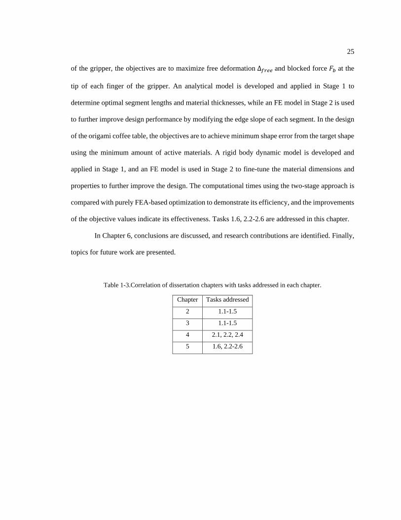
25

of the gripper, the objectives are to maximize free deformation ∆𝑓𝑟𝑒𝑒 and blocked force 𝐹𝑏 at the

tip of each finger of the gripper. An analytical model is developed and applied in Stage 1 to

determine optimal segment lengths and material thicknesses, while an FE model in Stage 2 is used

to further improve design performance by modifying the edge slope of each segment. In the design

of the origami coffee table, the objectives are to achieve minimum shape error from the target shape

using the minimum amount of active materials. A rigid body dynamic model is developed and

applied in Stage 1, and an FE model is used in Stage 2 to fine-tune the material dimensions and

properties to further improve the design. The computational times using the two-stage approach is

compared with purely FEA-based optimization to demonstrate its efficiency, and the improvements

of the objective values indicate its effectiveness. Tasks 1.6, 2.2-2.6 are addressed in this chapter.

In Chapter 6, conclusions are discussed, and research contributions are identified. Finally,

topics for future work are presented.

Table 1-3.Correlation of dissertation chapters with tasks addressed in each chapter.

Chapter Tasks addressed

2 1.1-1.5

3 1.1-1.5

4 2.1, 2.2, 2.4

5 1.6, 2.2-2.6

26

Chapter 2

Finite Element Analysis of EAP and MAE Actuation for Origami Folding

Using Continuum Modeling

[Most of the contents of this chapter were published in the following journal [68]: Zhang, W., Ahmed, S.,

Masters, S., Ounaies, Z., and Frecker, M., 2017, “Finite Element Analysis of Electroactive Polymer and

Magnetoactive Elastomer Based Actuation for Origami Folding,” Smart Mater. Struct., 26(10), p. 105032.]

2.1 Introduction and Motivation

The incorporation of smart materials, such as electroactive polymers (EAPs) and

magnetoactive elastomers (MAEs), can result in active folding of origami structures when using

external electric and magnetic stimuli, showing promise in many origami-inspired engineering

applications. In this dissertation, 3-D finite element analysis (FEA) models are developed for

several configurations that incorporate a combination of active and passive material layers,

namely,: 1) a single-notch unimorph folding configuration actuated using only external electric

field, 2) a double-notch unimorph folding configuration actuated using only external electric field,

and 3) a bifold configuration which is actuated using multifield (electric and magnetic) stimuli. A

unimorph is defined as an actuator which is composed of a layer of active material and a layer of

passive material. A bimorph, which is discussed in Chapter 3, is defined as an actuator which is

composed of two layers of active materials and one layer of passive material.

The objectives of this chapter are to develop and validate FEA models that simulate folding

behavior and to investigate the influence of geometric parameters on folding performance.

Equivalent mechanical pressures and surface stresses are used as external loads in FEA to simulate

27

electric and magnetic fields, respectively. By investigating the impact of geometric parameters and

locations of smart materials, FEA can be used in the design process, avoiding trial-and-error

iterations of experiments.

The following tasks are addressed in this chapter:

Task 1.1 Model the actuation mechanism of an EAP, namely, PVDF-based

terpolymer.

Task 1.2 Model the actuation mechanism of the MAE.

Task 1.3 Develop finite element models for single-field and multifield actuation of

active origami structures.

Task 1.4 Validate the FEA models using several folding configurations.

Task 1.5 Investigate influence of relevant structural parameters on the folding

performance of the active structures.

2.2 Actuation Mechanisms and Simulation Methods

2.2.1 Terpolymer Based Actuation

The relaxor ferroelectric P(VDF-TrFE-CTFE) terpolymer exhibits electrostrictive

response. When an electric field is applied through the thickness of the material, there is a

contraction in that direction followed by a corresponding expansion in the transverse directions. To

simulate the electric-field-induced strain 휀33, an equivalent surface traction 𝜏33 in the 3-direction

is deduced using Equation 2-1:

𝜏33 = 𝑌3333휀33 (2-1)

where the strain 휀33 is measured experimentally as a function of electric field; 𝑌3333 is the elastic

modulus in the thickness direction; and 𝜏33 is the compressive pressure used in the FEA model to

28

simulate the effects of the electric field. The assumption is made that the terpolymer film is isotropic

and expands in the 1-2 plane according to Poisson’s ratio when the material experiences contraction

in the thickness, as shown in Figure 2-1.

Figure 2-1. Compressive pressures are applied through the 3 direction as indicated by red arrows, and the

hollow arrows show the directions of planar expansion in the 1-2 plane.

In continuum modeling, we use the law of balance of linear momentum, which shows:

𝜌�̇� = div𝝈 + 𝒃0 (2-2)

where 𝜌 is the mass density, 𝒗 is the velocity, 𝝈 is the stress and 𝒃0 is the body force. In this

dissertation, we focus on predicting the final deformed shapes of different configurations upon

application of external fields regardless of the timing and trajectory of the object; therefore, the

assumption is made that all the studies in this dissertation obey the quasi-static assumption, thus 𝒗

is always zero. The only body force is the weight of the object. The balance of linear momentum

is expressed as shown in Equation 2-3:

div𝝈 + 𝜌𝒈 = 0 (2-3)

where 𝒈 is the gravitational acceleration, along with the boundary condition on the top and bottom

surfaces of the terpolymer as shown in Equation 2-4:

𝝈𝐧 = −𝜏33𝐧 (2-4)

An assumption is made that the terpolymer is within the linear elastic regime for the

deformations studied in this dissertation, which is further discussed in Section 2.3.2. Then the

matrix form of the constitutive relations of the deformation of the terpolymer are shown in Equation

2-5:

29

[ 𝜎1

𝜎2

𝜎3

𝜎4

𝜎5

𝜎6]

=

[ 𝜆 + 2𝜇

𝜆𝜆000

𝜆𝜆 + 2𝜇

𝜆000

𝜆𝜆

𝜆 + 2𝜇000

0002𝜇00

00002𝜇0

000002𝜇]

[ 휀1

휀2

휀3

휀4

휀5

휀6]

(2-5)

where the parameters 𝜆 and 𝜇 are expressed as:

𝜆 =𝑌𝜐

(1 + 𝜐)(1 − 2𝜐), 𝜇 =

𝑌

2(1 + 𝜐).

Where 𝜐 is Poisson’s ratio and 𝑌 is the elastic modulus. Because all the materials are assumed to

be isotropic, the elastic modulus in all directions are equal and denoted as 𝑌.

A unimorph actuator is made by attaching a passive material layer, or substrate, to the

terpolymer film, as depicted in Figure 2-2. When an electric field is applied to the terpolymer, its

planar expansion will be restricted by the substrate, thus resulting in bending behavior of the

structure.

The FEA models are developed using 3-D brick continuum elements from the solid

mechanics module of the commercial FEA package COMSOL Multiphysics. The solid mechanics

module is based on solving Navier’s equation, and results such as displacements, stresses and

strains are computed. 3-D brick continuum elements are adopted for two reasons. First, brick

elements conform to the cuboid shape of the target objects in this research, resulting in easier mesh

quality control. Second, brick elements have more degrees of freedom with a lower number of

elements compared to tetrahedral elements, and therefore are capable of reducing computational

errors and helping convergence especially for large deformation.

In the FEA, the active terpolymer layer and the passive layer are modeled as a union with

subdomains, which means that the contacting boundaries of the two layers are automatically

subjected to a continuity boundary condition while different material properties can be assigned to

the two layers.

30

Figure 2-2. The schematic of terpolymer-based unimorph bender.

2.2.2 MAE Based Actuation

Details on the magnetic material and its fabrication are discussed in our research group’s

previous work [69] and are briefly summarized here. To fabricate the MAE patches, 30% by

volume 325-mesh barium hexaferrite particles (ESPI Metals, Oregon) were embedded into PDMS

(Dow Corning sylgard 184, Michigan) matrix. First the samples are magnetically poled, and then

a vibrating sample magnetometer (VSM) is used to quantify their remanent magnetization. Once

placed in a magnetic field, the MAE patch will generate a torque. The magnetic torque generated

by a unit volume of MAE, which is denoted as 𝑻, can be calculated using Equation 2-6:

𝑻 = 𝑴 × 𝜇0𝑯 (2-6)

where 𝜇0 is the magnetic permeability of vacuum, 𝑴 is the remanant magnetization vector of the

particles per unit volume and 𝑯 is the external magnetic field vector. The assumption is made here

that the deformation is concentrated in the flexible regions representing creases, while the

deformation in the stiffer MAE patches is relatively small. Additionally, the concentrated

deformation, namely, the folding, takes place along a certain axis. Therefore, this cross-product can

be approximated as:

𝑇 = 𝜇0𝑀𝐻𝑠𝑖𝑛(𝛼) (2-7)

31

where 𝛼 is defined as the angle between the remanent magnetization (𝑴) and applied magnetic

field vectors (𝑯).

Since torques cannot be applied directly in the Solid Mechanics module of COMSOL, an

equivalent pair of surface tractions are applied to simulate the magnetic torque as shown in Figure

2-3. The pair of surface tractions are of the same magnitude 𝜏 but of opposite directions, creating a

net moment 𝑇′ as shown in Equation 2-8:

𝑇′ = 𝜏𝐴𝑡 (2-8)

where t is the thickness of the MAE patch and A is the surface area. When the angle between M

and H is 𝛼 , the tangent component of the surface stresses, which generates the torque,

becomes 𝜏sin (𝛼), and the corresponding magnetic torque becomes:

𝑇′ = 𝜏sin (𝛼)𝐴𝑡 (2-9)

which is consistent with the cross-product in Equation (2) by incorporating a sin (𝛼) term.

Figure 2-3. A pair of horizontal surface loads 𝜏 are applied on the top and bottom surfaces of MAE patch

orienting (a) horizontally and (b) with an angle 𝛼 to the field.

The actual magnetic torques 𝑇 under specified field strengths are calculated using Equation

1. By letting 𝑇 = 𝑇′, the values of the surface stresses 𝜏 in the FEA model are determined by

Equation 2-10:

𝜏 = 𝑇/(𝑡𝐴) (2-10)

32

The law of balance of linear momentum holds for MAE as well, as expressed in Equation

2-3. Now the boundary condition on the top and bottom surfaces of the MAE is:

𝝈𝐧 = 𝜏 (2-11)

The MAE is assumed to be an isotropic linear elastic material, and the constitutive

equations for the MAE are in the same format as shown in Equation 2-5 with appropriate material

properties.

2.3 FEA Modeling and Verification

In this section, several origami-inspired bending/folding configurations are used to validate

the FEA models through comparison with experiments, including terpolymer-based unimorph

bender, single-notch unimorph, double-notch unimorph and a multifield bifold configuration which

is actuated using both terpolymer and MAE.

2.3.1 Terpolymer-Based Unimorph Bender

The unimorph bender here is composed of a terpolymer layer and a scotch tape substrate

layer, as shown in Figure 2-2. The unimorph bender is used as a test model for its simplicity and

thereby the reliability and repeatability in experiments. Measurement of the material properties was

conducted by Ahmed and are described here. The tensile modulus of the terpolymer is measured

using a Dynamic Mechanical Analysis (DMA) machine of model RSA-G2 by TA Instruments. The

longitudinal strain 휀33 is measured through the thickness actuation experiments [30], which is

briefly summarized here. Voltage is applied on 1.2 𝑐𝑚 diameter, 30 𝜇𝑚 thickness electroded

terpolymer samples. Displacement in the thickness direction is measured and converted into strain

휀33, as recorded in Figure 2-5. More details on experiment and date can be found in [30]. The

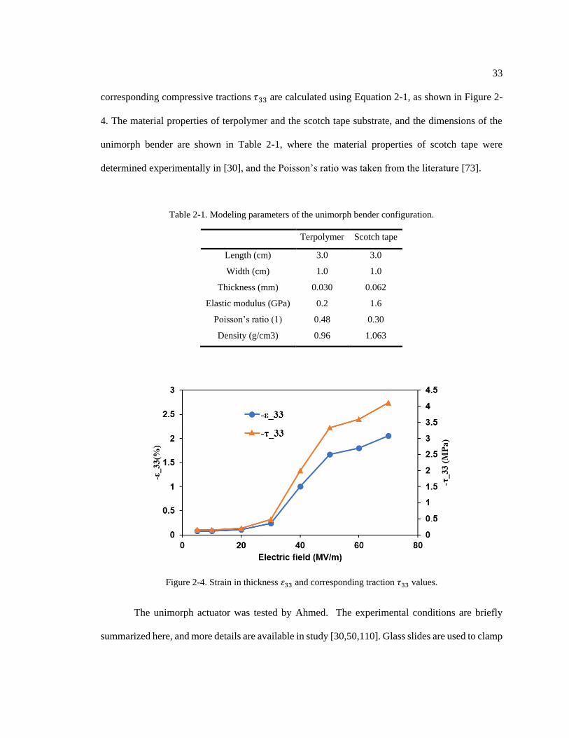
33

corresponding compressive tractions 𝜏33 are calculated using Equation 2-1, as shown in Figure 2-

4. The material properties of terpolymer and the scotch tape substrate, and the dimensions of the

unimorph bender are shown in Table 2-1, where the material properties of scotch tape were

determined experimentally in [30], and the Poisson’s ratio was taken from the literature [73].

Table 2-1. Modeling parameters of the unimorph bender configuration.

Terpolymer Scotch tape

Length (cm) 3.0 3.0

Width (cm) 1.0 1.0

Thickness (mm) 0.030 0.062

Elastic modulus (GPa) 0.2 1.6

Poisson’s ratio (1) 0.48 0.30

Density (g/cm3) 0.96 1.063

Figure 2-4. Strain in thickness 휀33 and corresponding traction 𝜏33 values.

The unimorph actuator was tested by Ahmed. The experimental conditions are briefly

summarized here, and more details are available in study [30,50,110]. Glass slides are used to clamp

34

the top part of the sample, which forms a fixed boundary condition as shown in Figure 2-11, except

that the sample here is a unimorph bender instead of a single-notch unimorph.

The meshed FEA model is shown in Figure 2-5. A fixed boundary condition is applied at

the top surfaces of the terpolymer and scotch tape to match the experimental conditions. The

compressive surface tractions 𝜏33 are applied in pair on the two large surfaces of the terpolymer.

Figure 2-5. The meshed FEA model of the terpolymer-based unimorph bender.

Deformed shapes from both the experiments and simulations are shown in Figure 2-6. In

the experiment the sample bends up as the electric field increases from 30 MV/m to 70 MV/m. It

can be observed that the 3-D continuum model is able to capture the bending behavior of the

unimorph bender, but for all electric fields, the simulation underestimates the bending curvature. It

is noted that Figure 2-6 shows results from only one set of experiments, which may not be

representative of the average performance. Therefore, comparison between the FEA and the

average results of repeated experiments is necessary.

To quantitatively compare experiments and FEA results, bending curvature is used as the

metric to determine how well the simulation matches the experiments, and is measured using the

image analysis software ImageJ. The bending curvature is measured as the following procedure. In

software ImageJ, a circle is created and adjusted to overlap the bending region. Then, the radius of

35

the circle is obtained from ImageJ in unit of pixel. Finally, the pixel count is converted into meters

with assistance of a reference object of a known length.

Figure 2-6. Deformed shape comparison of the unimorph bender between experiment (top) and simulation

(bottom) under specified electric fields.

The results are shown in Figure 2-7. The error bars in the experimental data indicate

plus/minus one standard deviation for a total of 8 samples measured. The FEA agrees well with the

experiments when the fields are 30, 40 and 50 MV/m, but underestimates bending curvature when

fields are 60 and 70 MV/m. The larger error bars at the moderate electric fields 40 and 50 MV/m

magnitudes indicate the dependence of folding performance on the fabrication of the unimorph

samples. For example, different thicknesses of the terpolymer from different fabrication batches

can lead to a change in bending stiffness and curvature of the composite beam. For the 8 bender

samples, the thickness of the terpolymer film ranges from 29 to 40 microns, while in the FEA

model, thickness of the terpolymer is estimated as 30 microns. A better consistency between the

samples is expected to improve the agreement between FEA and experimental results. In addition,

the FEA underestimates the bending curvature when 𝐸 = 60 and 70 MV/m, which indicates the

limitation of the continuum FEA method for the case of high bending curvature.

36

Figure 2-7. Comparison of bending curvature between experiment and simulation for the unimorph bender

with electric field ranging from 30 to 70 MV/m.

2.3.2 Single-notch Folding Configuration

Active folding can be achieved by taking advantage of a non-uniform thickness distribution

along the length of the substrate, as shown in Figure 2-8 (a). In general, the regions with thicker

passive material exhibit less bending curvature due to larger bending stiffness, and thus are called

“panels”. The regions with thinner passive material experience larger bending curvature and are

called “notches”. Under actuation, the deformation will be localized in the notches and in such a

way the folding performance is achieved, as shown in Figure 2-8 (b).

(a) (b)

Figure 2-8. Schematics of (a) a single-notch unimorph, and (b) the expected folding deformation in red, and

the original position in black.

37

A particular way to realize this non-uniformity is to add different numbers of layers of

passive material in certain regions of the structure. Figure 2-8 (a) shows a schematic of single-notch

folding configuration, where an adhesive scotch tape is attached to the terpolymer layer as the

passive material substrate. The material properties and geometric dimensions are listed in Table 2-

2.

Table 2-2. Modeling parameters for single-notch folding configuration.

Terpolymer Scotch tape

Length (cm) 6.0 6.0 (2.5 for panel, 1.0 for notch)

Width (cm) 2.0 2.0

Thickness (mm) 0.040 0.062 (single layer)

Elastic modulus (GPa) 0.2 1.6

Poisson’s ratio (1) 0.48 0.3

Density (g/cm3) 0.96 1.063

The experiments of the notched unimorph were conducted and the photos were taken by

Ahmed and are briefly summarized here, and the experimental date were used to validate the FEA

models. More details are available in [30,110]. The top of the sample was taped to a glass slide

vertically to produce a cantilever as seen in Figure 2-9 (a).

(a) (b)

Figure 2-9. The unimorph sample is attached to the glass slide to give the sample a cantilever constraint. (a)

Front view, (b) Side view. Photos were taken by Ahmed.

38

The terpolymer layer and scotch tape are modeled as isotropic materials. All these parts are

combined into a single union in the FEA model, making the contacting surfaces subject to a

continuity boundary condition. In order to reduce the degrees of freedom of the model and save

computing time, a symmetry boundary condition is applied in the center of the y-z plane, resulting

in a half-symmetry model with width of 1 cm instead of 2 cm. The dimensions and material

properties are listed in Table 2-2. As the sample is placed in the vertical direction, gravity is

assigned in the z-direction in the FEA model.

The meshed FEA model is shown in Figure 2-10 (a), with the notch region magnified in

Figure 2-10 (b). Since the localized deformation in the notch region will cause large bending

curvature, more elements are needed there to ensure relatively small deformation in each individual

element and a higher accuracy in the overall simulation results.

The effect of mesh density in the notch region is studied to find the least number of

elements that gives convergent simulation results. Here, an electric field of 70MV/m is applied in

the FEA model of the single-notch unimorph. Since the notch region is critical for folding behavior,

the average curvature 𝜅 in the notch is selected as the metric for mesh convergence, which is

measured in the FEA software package COMSOL Multiphysics with the selection of line average

principal curvature. The corresponding CPU time to converge for each FEA model is also recorded

to reveal the computational cost as a function of the degrees of freedom of the model. The FEA

result is shown in Figure 2-11, and as can be seen, the degrees of freedom increase with increasing

number of elements along the notch.

39

(a) (b)

Figure 2-10. The single-notch folding structure is meshed with brick elements. In the notch region the

elements are two times denser than in panel regions along the vertical direction. (a) The entire meshed

structure, and (b) meshed notch region.

Figure 2-11. Average curvature 𝜅 in the notch and the CPU time as functions of degrees of freedom of the

FEA model. The red dots show the least number of elements that lead to convergence.

From around 50,000 to 64,000 degrees of freedom (DoFs), the average curvature in the

notch increases dramatically. After 64,000 degrees of freedom, the fluctuation in average curvature

is less than 1%, so that beyond 64,000 degrees of freedom the model is assumed to converge. The

corresponding mesh density is 30 elements per centimeter in the notch and 10 elements per

centimeter in the panels. This mesh density is also adopted in the later double-notch folding model.

In this study, the model with DoFs 50000, 64000 and 89000 consume 1.8 hours, 4 hours and 7.2

hours to converge, respectively.

panel

panel

notch

40

According to beam theory, the maximum strain which appears on the surface of a beam is

calculated as in Equation 2-12:

휀 = 𝜅 ∙ 𝑑 (2 − 12)

where 𝑑 is the distance from the neutral axis to beam surface. Here, we let 𝜅 = 127/𝑚, as obtained

from Figure 2-11, which is representative for the bending and folding deformations appearing in

this dissertation, and 𝑑 = 60 𝜇𝑚 based on geometry of the unimorph, which leads to 휀 = 0.76%.

According to [111], the linear elastic regime of the terpolymer is within 3%, and therefore, the

assumption of linear elastic material of the terpolymer is justified.

The electric field magnitudes applied in the folding experiments are not exactly the same

as those applied in the strain test listed in Figure 2-4, so linear interpolation is utilized for the

calculation of compressive pressures to compare with experiment.

Figure 2-12. Deformed shape comparison between experiment (top) and simulation (bottom) under

specified electric fields and corresponding pressures.

Deformed shapes from both experiment and simulation are shown in Figure 2-12. It can

be observed that the sample folds up as the electric field increases from 25.0 MV/m to 62.5 MV/m.

It can be seen that a localized deformation occurs in the notched region where the bending stiffness

is lower than that of the panels, while the panels deformed much less. At 62.5 MV/m, the ends of

41

the two panels are in contact, which prevented the sample from further folding. The 3-D simulation

is able to capture the large localized curvature in the notch region, which occurs due to the reduction

of bending stiffness in the thinner notch region. However, it is also observed that at lower electric

fields like 25 MV/m and 37.5 MV/m, the simulation underestimates the folding somewhat, while

at higher fields like 62.5 MV/m, the folding is overestimated with the tip panel curling past the root

panel in the FEA.

In previous studies [30,89], tip displacement was considered an important metric to

compare experiment and simulation. However, it is not appropriate to use tip displacement when

the structure folds up and contacts itself under high electric fields, as shown in Figure 2-12. For

example, the experimental results at 62.5 MV/m show that the structure experiences greater folding

than 56.2 MV/m, but smaller tip displacement. For that reason, the folding angle is used as the

metric to determine how well the simulation matches experiments. Figure 2-13 shows the schematic

of how the folding angle is defined in this dissertation. The folding angle 𝜃 is measured as follows:

draw tangent lines at the two center points of both the root and the tip panels, extend them so that

they intersect, then measure the exterior angle of the angle that is between the two panels. The

image analysis software ImageJ is used to measure the folding angles for both experiments and

FEA results.

Figure 2-13. Folding angle 𝜃 is defined as the exterior angle between two lines that connect either end of

the sample to the closer edge of the notch.

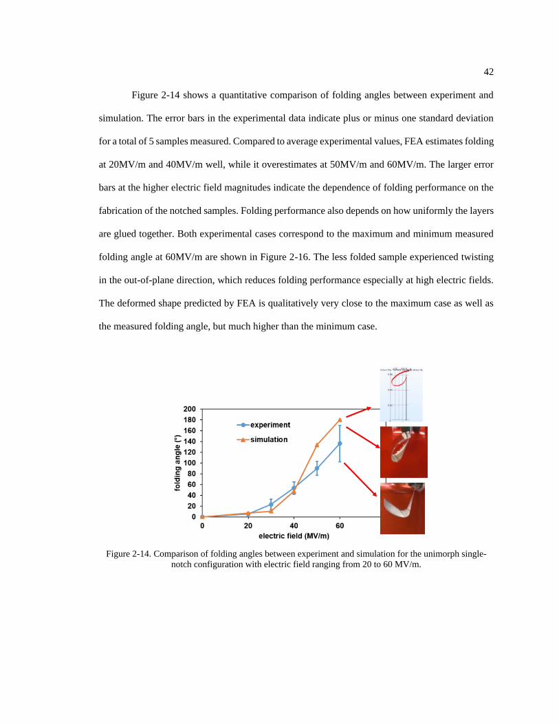
42

Figure 2-14 shows a quantitative comparison of folding angles between experiment and

simulation. The error bars in the experimental data indicate plus or minus one standard deviation

for a total of 5 samples measured. Compared to average experimental values, FEA estimates folding

at 20MV/m and 40MV/m well, while it overestimates at 50MV/m and 60MV/m. The larger error

bars at the higher electric field magnitudes indicate the dependence of folding performance on the

fabrication of the notched samples. Folding performance also depends on how uniformly the layers

are glued together. Both experimental cases correspond to the maximum and minimum measured

folding angle at 60MV/m are shown in Figure 2-16. The less folded sample experienced twisting

in the out-of-plane direction, which reduces folding performance especially at high electric fields.

The deformed shape predicted by FEA is qualitatively very close to the maximum case as well as

the measured folding angle, but much higher than the minimum case.

Figure 2-14. Comparison of folding angles between experiment and simulation for the unimorph single-

notch configuration with electric field ranging from 20 to 60 MV/m.

43

2.3.3 Parametric Study using FEA

A parametric study is conducted with the FEA to investigate the impact of geometric

parameters, including notch length, beam length and beam aspect ratio, on the folding performance.

The geometry of the beam in each case is denoted as beam length-width-notch length in

centimeters. In the notch length study, the length of the notch region varies from 0.5 cm to 4.0 cm,

while the beam length is kept constant at 6 cm. Folding angles and some typical deformed shapes

by FEA are shown in Figure 2-15.

Figure 2-15 shows that at a given electric field, the folding angle increases with an increase

in notch length. According to beam theory, the angular deflection 𝜃0 is calculated as shown in

Equation 2-12:

𝜃0 = 𝜅𝑙 (2 − 12)

where 𝜅 is the bending curvature and 𝑙 is the beam length. From Figure 2-12, we see that the folds

are localized in the notched regions where much higher bending curvatures are observed compared

to the panels. As the length of a notch increases, the folding angle, i.e., 𝜃0, will also increase.

Additionally, the increase in the length of the notch region shortens the length of the panels, which

leads to a smaller bending curvature in the panel regions. We can conclude that the notch geometry

plays an important role in folding performance and target folding angles could be achieved by

designing proper notch length.

44

Figure 2-15. Folding angles and deformed shapes in notch length study are shown, where the length of

notch changes from 0.5 to 4cm, while the length and width of the beam remain 6cm and 2cm respectively.

In the beam length study, the total length of the beam is studied at 3 cm, 6 cm to 9 cm,

while the ratios of beam length and beam width, beam length and notch length and also the

thicknesses of the materials are kept constant. Figure 2-16 shows that folding angle increases as the

beam length increases especially after 40MV/m. This trend can also be explained by Equation 2-

. With fixed material thicknesses, the bending curvature 𝜅 remains the same, and folding angle

increases with material length 𝑙.

In the beam width study, the width of the beam is varied from 1 cm, to 2 cm and to 4 cm,

while the beam length and notch length are kept constant at 6 cm and 1 cm, respectively. From

Figure 2-17, we can see that beam width does not have a significant effect on folding angle.

Compared with sample 6-1-1, sample 6-2-1 shows better actuation at 60 MV/m, but less actuation

at 50 MV/m. This may be due to numerical error in the FEA, i.e.,, there are jumps in the folded

shapes occurring at some loading steps in the FEA, whereas slight changes occur at other loading

steps. Here the step size of pressure is 0.1 MPa.

45

Figure 2-16. Folding angles in beam length study, where the length of the beam changes from 3cm to 9cm,

while the ratio of length-width-notch length remains constant.

Figure 2-17. Folding angles in beam width study, where the width of the beam changes from 1cm to 4cm,

while the length and notch length remain 6cm and 2cm respectively.

2.3.4 Double-notch Folding Configuration

As localized deformation and active folding are achieved successfully using the single-

notch configuration, a double-notch configuration was first proposed by Ahmed in order to realize

46

a higher overall extent of folding, and then is modeled here using FEA methods, as shown in Figure

2-18.

Since this active structure is actuated by terpolymer as well, the same modeling method is

utilized to apply pressures on the large surfaces of terpolymer film to simulate the effect of electric

field. The values of pressures at specified fields are listed in Figure 2-4. As with the single-notch

configuration, the sample is placed in the vertical direction; therefore, gravity is assigned in the z–

direction in the FEA model.

Figure 2-18. The schematic of double-notch folding structure.

The mesh density is the same as described in the last section, which is 30 brick elements

per centimeter in the notch regions and 10 elements per centimeter in the panels. The folding angle

measurement for each notch follows the same procedure as depicted in Figure 2-13. The deformed

shape and folding angle comparisons are shown in Figures 2-19 and 2-20, respectively. In this

simulation, the computation was terminated before reaching 2.8 MPa pressure, i.e.,, 46.1 MV/m of

electric field due to the large computer memory required for this geometrically more complex

structure.

47

Figure 2-19. Comparison of deformed shapes between the experiments and simulation for the double-notch

configuration.

Figure 2-20. Comparison of folding angle between experiment and simulation for both notch 1 and notch 2.

From both Figures 2-19 and 2-20, the experimental folding angles of the two notches at a

specified electric field are almost the same, which makes sense according to the symmetric

distribution of the two notches along the sample. Compared to the single-notch configuration,

folding angles are higher in double-notch case. For example, at 40 MV/m, the folding angle is about

50 degrees for the former and around 80 degrees for the latter. Hence, the double-notch

configuration exhibits much higher folding actuation than single-notch. Comparing with FEA, the

deformation in two notches in experiments are both much greater than that of FEA results before

48

40 MV/m, while at 46 MV/m FEA overestimates notch 1 but still underestimates notch 2. The

difference between notch 1 and notch 2 is due to the net force generated by the imbalance of the

compressive pressures acting on the two surfaces, which will be further discussed below.

One limitation of continuum FEA modeling is that the resultant forces acting on the two

large surfaces of the terpolymer due to the compressive tractions become unbalanced when the

unimorph deforms and leads to a difference in surface area between top and bottom side of

terpolymer layer. Although the unbalanced net forces are as small as several milli-Newtons, the

terpolymer and tape layers are so thin that the net force can cause substantial deformation. This

limits the range of stimuli magnitudes that can be applied in the model. Another limitation in FEA

is that both the terpolymer and scotch tape films are treated as linear isotropic materials with

properties independent of external environment, such as temperature, and the deformation process.

The terpolymer film may heat up when the electric field is applied due to dielectric losses, and thus

could experience changes in Young’s modulus and Poisson’s ratio. Also, the large bending

curvature occurs in the notch region, which may lead to a non-linear mechanical behavior of both

active and passive layers.

2.3.5 The Bifold Configuration

Most smart structures include a single type of active material as the actuator and respond

to a single external stimulus. The deformed shape depends only on the magnitude of that stimulus.

However, multifield responsive smart structures contain more than one type of active material and

are capable of folding to multiple target shapes depending on not only the magnitudes of the stimuli,

but also the types of stimuli that are applied. The bifold configuration, proposed by Dr. Landen

Bowen in [8], is a multifield responsive structure fabricated by Corey Breznak from by attaching

MAE patches and terpolymer strips onto the top and bottom surfaces of a polydimethylsiloxane

49

(PDMS) substrate, respectively, as shown in Figure 2-21. The MAE patches respond to external

magnetic field to fold the structure along one crease, while terpolymer films react to electric field

to give rise to folding along the other orthogonal crease. The fabricated samples of the bifold are

shown in Figure 2-22.

(a) (b)

Figure 2-21. Design of the bifold. In (a) top view, MAE patches are displayed with the shown poling

directions, leading to a fold about the vertical crease line. In (b) bottom view, four single-layer terpolymer

films are attached to give rise to folding about the horizontal crease line.

Figure 2-22. Four MAE patches (left) and four single-layer terpolymer actuator strips (right) are placed on

a PDMS substrate to create a multifield bifold. Since the PDMS is transparent, the sample edges are

highlighted in black [112].

The remanent magnetization M of the MAE with dimensions shown in Table 2-3 was

measured using a Microsense EZ7 vibrating sample magnetometer, which is 0.000367 𝐴 𝑚2⁄ . The

actual magnetic torques 𝑇 under specified field strengths are calculated using Equation 2-1, and the

values are shown in Figure 2-23. The values of the surface tractions 𝜏 in the FEA model are

determined by Equation 2-6, and shown in Figure 2-23.

50

Table 2-3. Material properties and dimensions of MAE patches.

MAE

Length (mm) 18.0

Width (mm) 18.0

Thickness (mm) 0.508

Density (g/cm3) 1.53

Elastic modulus (MPa) 3.5

Figure 2-23. Values of magnetic torque 𝑇 and corresponding surface stresses at different magnetic fields.

Due to the symmetry of the bifold configuration along both of the folding creases, the FEA

model is developed only for a quarter of the whole structure, as shown in Figure 2-24. A symmetry

boundary condition is applied on the surface with the arrows.

(a) (b)

Figure 2-24. Quarter symmetry FEA model of the bifold structure in (a) top view with an MAE patch and

in (b) bottom view with two terpolymer films. The arrows indicate the symmetry boundary condition

applied on that surface.

51

The experiments on the bifold configuration were conducted by Dr. Landen Bowen and

Kara Springsteen. More details can be found in [112]. As the magnetic field is applied from left to

right (assuming the same orientation as found in Figure 2-25), the MAE will try to align with the

applied field. This results in the left and right sides rotating out of the page, forming a “V” (see

Figure 2-25). The sample was tested inside a large horizontally-oriented Walker 7HF

electromagnet, and the actuation angle of the sample was measured from digital images taken as

the magnetic field strength was varied from 0.0083 to 0.1195 T (see Figure 2-23). Three tests over

the range of field strengths were performed on the same sample. The magnitudes of magnetic

torques each MAE patch experiences under different field strengths are reported in Figure 2-23,

where using Equation 2-6, the corresponding surface loads are calculated and shown in Figure 2-

23. Since the folding happens in the vertical plane, gravity is assigned in the z– direction.

Figure 2-25. The bifold was placed inside of a large, horizontally oriented electromagnet. Upon application

of a magnetic field, the MAE patches rotate to fold the PDMS substrate as they attempt to align with the

applied field [112].

Upon supply of power, the PDMS substrate folds along the crease line due to the actuation

of the MAE patches, which rotate to align with the magnetic field as shown in Figure 2-25. The

deformed shape in simulation is shown in Figure 2-26. Here 𝜃 represents half of the folding angle

because the FEA model is symmetric about the crease line, where the large local deformation is

evident.

52

Figure 2-26. The simulated image of the actuated quarter of bifold under field strength 0.1195 T. according

to the symmetry of bifold geometry, 𝜃 indicates half of the folding angle.

As we can see from Figure 2-27, the simulation results show good agreement with

experimental data in most cases except at very low magnetic field where the folding angle is

negative in simulation because of the overwhelming effect of gravity under such a small field

strength, while in the experiment the sample is supported by the platform on which it sits, and

therefore exhibits zero folding angle. The simulated values are generally about 5-10 degrees greater

than measured by experiment, for reasons which are discussed below.

Figure 2-27. Comparison of folding angle between simulation and experiment for MAE actuation of the

bifold.

53

The feasibility of this modeling method is validated by the good agreement between

simulation and experimental results in the bifold configurations. The 5-10-degree difference in the

simulated folding angles and experimental ones is attributed primarily to the reduction of the

magnetic field strength from the center of the magnets to the edge. The magnets are about 10 cm

in diameter, and the bifold sample is 45mm in length and width. According to our measurement,

the magnetic field is 121 mT at the center, and 115 mT at the position 2cm away from the center,

showing a 5% reduction in field strength. Another reason for the difference is that the adhesive

layer between the terpolymer films and the PDMS are not included in the FEA model, which may

lead to a slight over prediction of the folding angles using FEA.

In addition to the MAEs, terpolymer films were added to make a multifield actuated bifold.

The terpolymer actuators were fabricated using a single layer of electroded terpolymer. After

fabrication, adhesive spray (scotch super 77) was used to attach the terpolymer to the PDMS

substrate. The sample was held using tweezers and oriented such that gravity did not oppose the

folding, and the wires were connected to a high voltage power supply (see Figure 2-28). A camera

was placed under the sample to take the videos as the applied electric field strength was increased

from 30 to 80 MV/m. Two different single-layer actuators were tested on the same substrate three

times each.

Figure 2-28. The bifold sample is hung using tweezers and folds in the horizontal plane for terpolymer

actuation.

x

z

y

54

For the terpolymer actuation, the values of the pressures are listed in Figure 2-4. In this

experiment the folding happens in the horizontal plane, the y-z plane in Figure 2-28; so, the gravity

is set to zero in the FEA model. The meshed FEA model is shown from the side where terpolymer

is attached, as in Figure 2-30. The mesh density is much higher in root region than in other parts in

order to reduce influence of stress concentration. The experimental setup and the deformed shapes

in both experiments and simulation are shown in Figures 2-29, 2-31 and 2-32 respectively. To

reduce the influence of stress concentration on the edge where fixed boundary condition is applied,

20 elements are assigned along the root region of 2.25 mm as shown in Figure 2-35, resulting in a

much higher mesh density than in other parts. Figure 2-34 shows the von Mises stress distribution

in the terpolymer strips and PDMS matrix.

(a) (b) (c)

Figure 2-29. Deformed shapes of the bifold actuated using electric field of (a) 0 MV/m, (b) 40MV/m and

(c) 70 MV/m.

(a) (b)

Figure 2-30. Overall mesh assignment viewed from the side of terpolymer films (a) and exaggerated root

region (b). The mesh density is much higher in root region than in other parts in order to reduce influence

of stress concentration.

55

Figure 2-31. The deformed shape in simulation under electric field of 70 MV/m for terpolymer actuation.

According to the symmetry of bifold geometry, 𝜃 is half of the folding angle.

Figure 2-32. The von Mises stress of terpolymer strips and PDMS matrix are shown.

From Figure 2-33 we can see that the average experimental folding angle increases as the

electric field increases from 30 MV/m to 70 MV/m, but decreases from 70 MV/m to 80 MV/m,

where breakdown of the terpolymer film is likely to be initiated. Large error bars are observed at

30 MV/m, 50 MV/m and 60 MV/m, indicating a large difference in actuation quality between the

two tested samples. The FEA results agree reasonably well with the experimental results from 30

MV/m to 60 MV/m, but clearly underestimate the folding at 70 MV/m. This difference is attributed

to three main reasons. First, the folding of bifold for the terpolymer-based actuation takes place

horizontally; so, ideally gravity has no effect on the folding performance and is not included in the

FEA model. But in the experiments, twisting of the sample is observed (see for example Figure 2-

29), which will result in weight aiding in the folding performance. Second, the values of the

56

compressive pressures to simulate the electrostrictive response are calculated based on

experimentally measuring the strain 𝑆33 for terpolymer films of thicknesses of ~30 microns.

However the terpolymer films used in the bifold are from a different batch of films, generally

thinner with thicknesses of ~26 microns; therefore, the former values of the pressures may be

underestimated in bifold actuation. Last, the elastic modulus of the MAE patches used in the FEA

model is likely higher than the measured value, which will stiffen the sample in the FEA model

and decrease the folding angles.

Figure 2-33. Comparison of folding angle between experiment and simulation for terpolymer actuation.

2.4 Summary

In this chapter, finite element analysis captured the folding performance of electric

actuation for notched configurations and multifield (magnetic and electric fields) actuation for a

bifold structure. Upon application of the external stimulus, folding of the panels occurs and

localized deformation is formed within notched or creased regions, which agrees well with

experiments. Quantitative comparison using the folding angle as the metric shows that FEA results

are comparable to experiments for terpolymer actuated single-notch and multifield bifold

configurations.

57

The geometric parameter studies show that folding angles will increase as the notch length

or beam length increases, and beam width does not have an appreciable effect on folding

performance. The curling phenomenon in notch region dominates folding when the notch length is

3 cm and 4 cm, i.e., 50% and 66.7% of the entire length of the unimorph. Based on the target folded

shapes and the range of available external stimuli, geometric parameters can be designed to meet

specific needs.

Overall, FEA continuum modeling can be a powerful tool to predict folding performance

of complex 3-D multifield responsive structures. Understanding the impact of geometric

parameters and locations of smart materials through FEA helps with preliminary design and reduces

the number of trial-and-error iterations in experiments. One limitation of this modeling method is

that the unbalanced compressive normal surface tractions caused by the application of a constant

pressure with increasing surface area upon folding of the structures, which may lead to some

deviation from experimental results, especially when the structure is very thin. Moreover,

improvement of the fabrication quality of the samples is expected to lead to better consistency in

the structural behavior and to better model validation.

58

Chapter 3

Finite Element Analysis of EAP and MAE Actuation for Origami Folding

Using Constitutive Modeling

[Most of the contents of this chapter were published in the following journal [113]: Zhang, W., Ahmed, S.,

Masters, S., Hong, J., Ounaies, Z. and Frecker, M., 2018. “Finite element analysis of electroactive and

magnetoactive coupled behaviors in multifield origami structures.” Journal of Intelligent Material Systems

and Structures, 29(20), pp.3983-4000.]

3.1 Introduction and Motivation

This chapter is focused on constitutive modeling to explicitly simulate the coupled behaviors

of electroactive and magnetoactive materials. Instead of continuum elements, shell elements are

adopted in the finite element models for their capacity to model thin films, reduction of

computational cost, and ability to model the intrinsic coupled behaviors in the active materials

under consideration. FEA results are then compared with experiments for multifield actuation, to

validate the models. In this chapter, FEA models are developed for several configurations that

incorporate a combination of active and passive material layers, namely: 1) a single-layer-

terpolymer-based unimorph bender, 2) a multilayer-terpolymer unimorph bender, 3) a single-notch

unimorph folding configuration actuated using terpolymer, 4) a terpolymer-based finger

configuration and 5) a bimorph configuration which is actuated using both electric and magnetic

(i.e., multifield) stimuli. The electrostrictive coefficients are measured and then used as material

properties in the constitutive modeling of the coupled behavior of the terpolymer material. The

magnetization of the MAE is measured and then used to calculate magnetic torque under specified

external magnetic field. The objective of the chapter is to verify the effectiveness of the constitutive

models implemented through the FEA method to simulate multifield coupled behaviors of the

active origami configurations.

The following tasks are addressed in this chapter:

59

Task 1.1 Model the actuation mechanism of PVDF-based terpolymer.

Task 1.2 Model the actuation mechanism of the MAE.

Task 1.3 Develop finite element models for single-field and multifield actuation of

active origami structures.

Task 1.4 Validate the FEA models using several simple folding configurations.

Task 1.5 Investigate influence of relevant structural parameters on the folding

performance of the active structures.

3.2 Constitutive Modeling and FEA Implementation

3.2.1 Terpolymer-based Actuation

The terpolymer is a relaxor ferroelectric material as introduced in Section 2-2-1. In general,

the electrostrictive response is modeled as a quadratic coupling between strain and electric field.

The expression of strain 휀𝑖𝑗 in terms of electric field 𝐸𝑘, 𝐸𝑙 and stress 𝜎𝑘𝑙 is shown as Equation 3-

1 [114]:

휀𝑖𝑗 = 𝑆𝑖𝑗𝑘𝑙𝜎𝑘𝑙 + 𝑀𝑖𝑗𝑘𝑙𝐸𝑘𝐸𝑙 (3-1)

where 𝑆𝑖𝑗𝑘𝑙 is the elastic compliance tensor and 𝑀𝑖𝑗𝑘𝑙 represents the electro-mechanical coupling

tensor. In this chapter, several assumptions are made based on experimental conditions and

observations. First, same as Chapter 2, all the materials considered are mechanically isotropic.

Second, the electric field is always applied through the thickness direction of the active material

layers, thus the only non-zero term in 𝐸𝑘 is 𝐸3 , where the 3-direction denotes the thickness

direction and the 1- and 2- directions denote in-plane directions. Third, there is no residual stress

60

when the material is at rest. Therefore, the constitutive relation, taking these assumptions into

consideration and written using the vector-matrix notation, becomes as shown in Equation 3-2:

휀𝐼 = 𝑆𝐼𝐽𝜎𝐽 + 𝑀𝐼𝐽𝐸𝐽2 (3-2)

For convenience of FEA implementation, the stress vector is expressed explicitly in terms

of the strain and coupling effects, as shown in Equation 3-3:

𝜎𝐽 = 𝑆𝐼𝐽−1(휀𝐼 − 𝑀𝐼𝐽𝐸𝐽

2) (3-3)

The expanded form of the equation above is shown in Equation 3-4:

[ 𝜎1

𝜎2

𝜎3

𝜎4

𝜎5

𝜎6]

=

[ 𝜆 + 2𝜇

𝜆𝜆000

𝜆𝜆 + 2𝜇

𝜆000

𝜆𝜆

𝜆 + 2𝜇000

0002𝜇00

00002𝜇0

000002𝜇]

(

[ 휀1

휀2

휀3

휀4

휀5

휀6]

−

[ 𝑀11

𝑀21

𝑀31

000

𝑀12

𝑀22

𝑀32

000

𝑀13

𝑀23

𝑀33

000

000

𝑀44

00

0000

𝑀55

0

00000

𝑀66]

[ 00𝐸3

2

000 ]

)

(3-4)

The parameters 𝜆 and 𝜇 are expressed as:

𝜆 =𝑌𝜐

(1 + 𝜐)(1 − 2𝜐), 𝜇 =

𝑌

2(1 + 𝜐).

in which 𝑌and 𝜐 are elastic modulus and Poisson’s ratio of the terpolymer, respectively, taking the

mechanical isotropy into consideration. In Equation 3-4, since the only non-zero component in

electric field vector is 𝐸3, the effective electrostrictive coefficients in this model which will have

impact on the coupled response of the terpolymer, are 𝑀13, 𝑀23 and 𝑀33. These coefficients will

be determined through experiments, which will be shown later in Section 3.3.1.

Due to the compliance of the terpolymer layer, it is not convenient to measure the

transverse strains 휀1 and 휀2 directly. In this chapter, the assumption is made that transverse strain

in 1- direction equals that in 2- direction, and the coefficient 𝑘 is defined as the ratio of the

61

transverse strain to the longitudinal strain, in magnitude, induced purely by external electric field,

namely:

𝑘13 = −휀11(𝑜𝑟 휀22)

휀33 (3 − 5)

And equivalently, it holds that:

𝑘13 = −𝑀11(𝑜𝑟 𝑀22)

𝑀33 (3 − 6)

The FEA model is developed using the shell module of the COMSOL Multiphysics. There

are two main reasons to adopt shell elements. One is that shell theory is a good approximation for

the deformation of thin structures, in which the thickness is less than about 1/20 of the smallest

dimension of their midsurface [115]. By neglecting the normal and shear stresses in the thickness

direction, shell elements assume a plane stress condition and do not have nodes through thickness,

which significantly decrease the total number of nodes, and thus the degrees of freedom in the

model, compared to using solid elements. For the models introduced in this dissertation, the number

of degrees of freedom is typically decreased by two orders of magnitude by using shell elements

rather than continuum elements. The other advantage is that it is convenient to modify the

constitutive equations of shell elements in COMSOL for terpolymer-based actuation, and to apply

a body moment as input for the MAE-based actuation, which will be presented later in this chapter.

The shell elements used in COMSOL are of Mindlin-Reissner type, which means that

transverse shear deformation is accounted for [116]. They can thus also be used for rather thick

shells. The law of balance of linear momentum for a shell element is expressed as Equation 3-7:

div𝐓 + 𝜌𝐠 + 6(𝐌𝐯 × 𝐧)𝑧

𝑑= 0

and 𝛔𝐳 = 0,−0.5 ≤ 𝑧 ≤ 0.5. (3-7)

62

where 𝐓 denotes the stress tensor of the object, 𝐌𝐯 is the body moment applied on the object, d

denotes the thickness of the shell element, and 𝑧 is the relative level position with magnitude

ranging from -0.5 to 0.5 and zero at the midsurface. The term 6(𝐌𝐯 × 𝐧)𝑧

𝑑 represents the

contribution of external bending moments or twisting torques on the stress tensor 𝐓 at relative level

z in the shell element.

For terpolymer-based actuation, the constitutive equations of the shell elements are

modified according to Equation 3-4, in which the electro-mechanical coupling stress terms are

added to the original mechanical stresses, particularly the membrane components of second Piola-

Kirchhoff stresses in xx-, yy- and zz- directions with respect to local coordinate system in

COMSOL’s shell module. The modified stresses are shown in Equation 3-8.

𝜎1 = (𝜆 + 2𝜇)휀1 + 𝜆휀2 + 𝜆휀3 − [(𝜆 + 2𝜇)𝑀13 + 𝜆(𝑀23 + 𝑀33)] × 𝐸32

𝜎2 = (𝜆 + 2𝜇)휀2 + 𝜆휀1 + 𝜆휀3 − [(𝜆 + 2𝜇)𝑀23 + 𝜆(𝑀13 + 𝑀33)] × 𝐸32 (3 − 8)

𝜎3 = (𝜆 + 2𝜇)휀3 + 𝜆휀2 + 𝜆휀1 − [(𝜆 + 2𝜇)𝑀33 + 𝜆(𝑀23 + 𝑀13)] × 𝐸32

3.2.2 MAE-based Actuation

When an MAE material is placed in an external magnetic field, it will experience a

magnetic torque, which always tries to align the magnetization direction with the external magnetic

field direction. The magnetic torque 𝑇 for a unit volume of particles is determined:

𝑻 = 𝑴 × 𝜇0𝑯 (3-9)

where 𝜇0 is the magnetic permeability of vacuum, 𝑴 is the remanent magnetization vector per

particle unit volume and 𝑯 is the external magnetic field vector. As the MAE patch rotates, the

63

direction of 𝑴 remains the same with respect to the surrounding polymer matrix, i.e.,, the material

coordinate system, but it changes correspondingly in global coordinate system. Now let the rotation

matrix of the MAE patch be 𝑹 from global coordinates to material coordinates, and let 𝑴𝒊𝒏𝒊 be the

initial magnetization vector in global coordinate system. Then the rotated 𝑴 is:

𝑴 = 𝑹𝑴𝒊𝒏𝒊 (3-10)

and the current magnetic torque for a unit volume is:

𝑻 = 𝑴 × 𝜇0𝑯 = (𝑹𝑴𝒊𝒏𝒊) × 𝜇0𝑯 (3-11)

An equivalent method to express 𝑹 is to use the displacement of the normal vectors of the

shell elements. In this chapter, the MAEs are poled in such a way that the magnetization 𝑴 is

normal to the surface. Let the initial normal vector of a MAE patch in global coordinate be:

𝒏𝟎 = [𝑛𝑥0, 𝑛𝑦0, 𝑛𝑧0]𝑇 (3-12)

Since 𝑴 is always along the normal vector 𝒏, then 𝑴𝒊𝒏𝒊 can be expressed as:

𝑴𝒊𝒏𝒊 = 𝑀0𝒏𝟎 = 𝑀0[𝑛𝑥0, 𝑛𝑦0, 𝑛𝑧0]𝑇 (3-13)

where 𝑀0 is the magnitude of 𝑴.

In the shell module of COMSOL, the rotation matrix 𝑹 can be simplified by taking

advantage of the unit normal vector, as shown in Figure 3-1. When a shell element rotates from its

original position, the displacement of the normal vector is expressed as:

𝒂 = [𝑎𝑥 , 𝑎𝑦 , 𝑎𝑧]𝑇 (3-14)

64

Figure 3-1. Rotation of a shell element can be interpreted using the displacement in unit normal vector.

So, the rotated unit normal vector is:

𝒏 = 𝒏𝒊𝒏𝒊 + 𝒂 = [

𝑛𝑥0 + 𝑎𝑥

𝑛𝑦0 + 𝑎𝑦

𝑛𝑧0 + 𝑎𝑧

] (3-15)

Then the rotated magnetization is:

𝑴 = 𝑀0𝒏 = 𝑀0 [

𝑛𝑥0 + 𝑎𝑥

𝑛𝑦0 + 𝑎𝑦

𝑛𝑧0 + 𝑎𝑧

] (3-16)

In general, the magnetic field strength can be expressed as:

𝑯 = [

𝐻𝑥0

𝐻𝑦0

𝐻𝑧0

] (3-17)

Substituting 𝑴 and 𝑯 into Equation 3-8, we have:

𝑻 = 𝑴 × 𝜇0𝑯 = (𝑀0 [

𝑛𝑥0 + 𝑎𝑥

𝑛𝑦0 + 𝑎𝑦

𝑛𝑧0 + 𝑎𝑧

]) × 𝜇0 ([

𝐻𝑥0

𝐻𝑦0

𝐻𝑧0

]) (3-18)

The magnitudes of the magnetic torques per unit volume in x, y and z directions are

calculated and shown in Equation 3-19:

𝑇𝑥 = 𝜇0𝑀0 [(𝑛𝑦0 + 𝑎𝑦)𝐻𝑧0 − (𝑛𝑧0 + 𝑎𝑧)𝐻𝑦0]

𝑇𝑦 = 𝜇0𝑀0 [−(𝑛𝑥0 + 𝑎𝑥)𝐻𝑥0 + (𝑛𝑧0 + 𝑎𝑧)𝐻𝑥0] (3-19)

65

𝑇𝑧 = 𝜇0𝑀0 [(𝑛𝑥0 + 𝑎𝑥)𝐻𝑦0 − (𝑛𝑦0 + 𝑎𝑦)𝐻𝑥0]

Assuming that the external magnetic field 𝑯 is constant and is in the positive z direction,

the decomposition of 𝑯 in the global coordinate system is:

𝑯 = 𝐻0[0, 0, 1]𝑇 (3-20)

where 𝐻0 is the magnitude of the field 𝑯.

𝑻 = 𝜇0𝑴 × 𝑯 = 𝜇0 (𝑀0 [

𝑛𝑥0 + 𝑎𝑥

𝑛𝑦0 + 𝑎𝑦

𝑛𝑧0 + 𝑎𝑧

]) × (𝐻0 [001])

= 𝜇0𝑀0𝐻0 [

𝑛𝑦0 + 𝑎𝑦

−(𝑛𝑥0 + 𝑎𝑥)

0

] (3-21)

In the shell module of COMSOL, we can directly apply a body torque density in x-, y- and

z- directions as input with unit N ∙ m/m3, particularly in this chapter:

𝑇𝑥 = 𝜇0𝑀0𝐻0(𝑛𝑦0 + 𝑎𝑦)

𝑇𝑦 = −𝜇0𝑀0𝐻0(𝑛𝑥0 + 𝑎𝑥) (3-22)

𝑇𝑧 = 0

The law of balance of linear momentum for the MAE is the same as the terpolymer-based

actuation as shown in Equation 3-7. Since the MAE is modeled as an isotropic linear elastic

material, the constitutive equations are given in Equation 2-5.

66

3.3 FEA Modeling and Verification

3.3.1 Terpolymer-based Unimorph Bender

As described in Chapter 2, the terpolymer-based unimorph bender is composed of a

terpolymer layer and a scotch tape layer attached together, as shown in Figure 2-2, with dimensions

as listed in Table 2-1.

The meshed FEA model is shown in Figure 3-2b. The terpolymer layer and scotch tape

layer are defined in two separate shell interfaces which share a single common shell layer in the

model; so, there is only one layer visible in the FEA model. By default, the shell layer represents

the position of the midsurface of the real layer in thickness direction, but the position of midsurface

can be relocated by setting a desired “offset”, as shown in Figure 3-2a. In this model, the terpolymer

is treated as the base of this composite beam of which the offset is set equal to zero. The offset of

the scotch tape attached to the terpolymer layer is set to:

𝑑𝑠𝑐𝑜𝑡𝑐ℎ1 = (𝑡𝑡𝑒𝑟 + 𝑡𝑠𝑐𝑜𝑡𝑐ℎ)/2 (3-22)

where 𝑡𝑡𝑒𝑟 and 𝑡𝑠𝑐𝑜𝑡𝑐ℎ denote the thickness of terpolymer layer and scotch tape layer respectively.

By using the same variable names in the displacement matrix, these two shell interfaces are

constrained so that they deform as a union. A parametric sweep study of the coefficient 𝑘 is

conducted to investigate its impact on bending curvature.

67

(a) (b)

Figure 3-2. A schematic of the shell model of the unimorph bender is shown as (a), where the

offset of the midsurfaces account for the thickness. The meshed FEA model for the bender is shown as (b).

To obtain the values of the coupling coefficients, Ahmed conducted experiments to

measure the longitudinal strain 휀3 induced by application of electric field where the terpolymer

sample is free from mechanical constraint, in other words, 𝜎𝐽 is zero. In this situation, the coupling

coefficient 𝑀33 can be calculated as in Equation 3-5, and the measured 휀3 and calculated 𝑀33 are

shown in Figure 3-3 as a function of electric field:

Figure 3-3. The measured longitudinal strain 휀33 and the calculated coupling coefficient 𝑀33are

shown with electric field ranging from 0 to 70 MV/m.

68

𝑀33 = 휀3 𝐸32⁄ (3-5)

Before simulation of the terpolymer-based actuation, the values of the ratio coefficient 𝑘

in Equation 3-6 and Equation 3-7 must be determined. In this chapter, k is determined empirically

using the unimorph bender configuration.

Deformed shapes of both experimental samples and FEA results are shown for electric

field ranging from 0 to 70 MV/m and the case 𝑘 = 0.7 in Figure 3-4. It can be seen that as electric

field increases, the bending curvature of the bender also increases in both experiments and FEA

results. In order to quantitatively compare FEA with experiments, the image analysis software

ImageJ is used to measure the bending curvature for both experiments and FEA results, and the

results are shown in Figure 3-5. The error bars on the experimental data represent plus or minus a

standard deviation which is obtained from 8 different samples and one test on each sample. The

bending curvature increases correspondingly with coefficient 𝑘, and from Figure 3-5 we can see that

the cases 𝑘 = 0.6 and 𝑘 = 0.7 match experiments fairly well. To determine the best approximation

of 𝑘, the normalized squared error between FEA and experiments is adopted as the criterion to

evaluate the overall deviation of FEA from the experiments for each k value. As a result, the FEA

model with 𝑘=0.7 leads to the lowest normalized error, which is 6.7%. Therefore, 𝑘=0.7 is

considered as the best approximation and is used in the remaining models in this paper. In this

dissertation, the coefficient 𝑘 is assumed to be a constant under different electric fields. In fact, 𝑘,

as a material property of the terpolymer, is likely to vary with electric field. However, we can see

from Figure 3-5 that the simulation results with 𝑘=0.7 are very close to the average values of

experimental data for high electric fields of 60 MV/m and 70 MV/m, and agree fairly well with

experimental data for low fields from 30 to 50 MV/m when the error bars are considered. Thus, the

assumption is justified.

69

The coefficient 𝑘, which is defined by the ratio between transverse strain to longitudinal

strain caused by the electro-mechanical coupling response, is determined as 0.7 to best match FEA

to experiments. The value 𝑘 = 0.7 is beyond the value of 0.5 for Poisson’s ratio under constant

volume assumption. In fact, the coefficient 𝑘 includes the electromechanical coupling response in

addition to the pure mechanical response; so, the value 0.7 for 𝑘 is assumed to be reasonable.

Figure 3-4. The deformed shapes of the unimorph bender are compared between experiments and

FEA.

Figure 3-5. The bending curvatures of the unimorph bender are measured for experiments and

FEA with 𝑘 varying from 0.5 to 0.9.

70

3.3.2 Multilayer Terpolymer Bender

A multilayer terpolymer can be used as the actuator in an active structure as shown in

Figure 3-6, in order to increase actuation force and displacement. To show this, 2-layer, 4-layer and

6-layer terpolymer-based benders are tested and simulated in this chapter.

Figure 3-6. The schematic of a unimorph bender actuated using double-layer terpolymer.

The terpolymer films are attached to each other using spray glue from 3M Corporation.

The glue layer increases the overall bending stiffness, but the elastic modulus and the thickness of

the glue layer cannot be easily measured experimentally. In this chapter, a parametric sweep study

is conducted to investigate the impact of the glue layer on bending curvature, where thickness

ranges from 1 µm to 20 µm and modulus ranges from 0.1 GPa to 2 GPa for the glue layer. The goal

is to find the particular set of thickness and modulus of the glue layer that leads to a good agreement

between FEA and experiments for all three cases, namely, 2-layer, 4-layer, and 6-layer terpolymer

based benders, at the same time. It was found that 𝑡𝑔𝑙𝑢𝑒 = 10𝜇𝑚 and 𝑌𝑔𝑙𝑢𝑒 = 1𝐺𝑃𝑎 are the

properties of the glue layer that minimize the difference between FEA and experiments

simultaneously for the cases of 2, 4 and 6 layers of terpolymer; the bending curvatures are compared

between FEA and experiments in Figure 3-7.

71

Figure 3-7. FEA results are compared with experiments in bending curvatures of 2-layer, 4-layer

and 6-layer terpolymer-actuated benders.

The material properties estimated in this chapter are assumed to be reasonable enough to

predict how much impact the glue layer exerts on the overall bending performance of the bending

actuator. A sensitivity study of the glue layer to the bending curvature is conducted, as shown in

Figure 3-8. It is found that when the thickness of the glue layer is doubled, the bending curvature

reduces by 7.9%, 18.0% and 18.0% for 2-layer, 4-layer and 6-layer terpolymer-based benders,

respectively. When the elastic modulus of the glue layer is doubled, the bending curvature reduces

by 1.0%, 13.7% and 18.6% for 2-layer, 4-layer and 6-layer terpolymer-based benders respectively.

Based on this sensitivity study, the glue layer overall exerts more influence on the 4-layer and 6-

layer bender than the 2-layer terpolymer bender, and thickness has more influence than the elastic

modulus on the bending of 2- and 4-layer terpolymer benders, but they seem to have the same

impact on the 6-layer bender. It is demonstrated that good estimates of the material properties of

the glue layer are necessary to accurately predict the deformation of the benders, especially for

multilayer terpolymer-based samples.

72

Figure 3-8. The sensitivity study of the glue layer to the bending curvature.

3.3.3 Single-notch Folding Configuration

As described in Section 2.3.2, active folding can be achieved by introducing non-uniform

thickness along the length direction of the sample, in which case localized bending occurs at the

thinner region, i.e., the notch region, to realize folding behavior. A schematic and fabricated sample

of a single-notch unimorph configuration are shown in Figures 2-9 and 2-9, and the dimensions are

listed in Table 2-2.

Similar to the FEA modeling in previous section, the terpolymer layer and two scotch tape

layers are defined as three separate shell interfaces which share a single common shell layer in the

model, and the terpolymer is treated as the base of this composite beam of which the offset is set

equal to zero. The offset of the scotch tape attached to the terpolymer layer is set to:

𝑑𝑠𝑐𝑜𝑡𝑐ℎ1 = (𝑡𝑡𝑒𝑟 + 𝑡𝑠𝑐𝑜𝑡𝑐ℎ)/2 (3-23)

and the offset of the patches of scotch tape is set to:

73

𝑑𝑠𝑐𝑜𝑡𝑐ℎ2 = (𝑡𝑡𝑒𝑟 + 3𝑡𝑠𝑐𝑜𝑡𝑐ℎ)/2 (3-24)

where 𝑡𝑡𝑒𝑟 and 𝑡𝑠𝑐𝑜𝑡𝑐ℎ denote the thickness of terpolymer layer and scotch tape layer respectively.

By using the same variable name in the displacement matrix, these three shell interfaces are

constrained so that they deform as a union. Since there will be localized higher deformation

occurring in the notch, the mesh density is doubled in that region as compared to in the panels.

Figure 3-9 shows the ability of the EFA model to simulate folding. In the original FEA

model, which includes the whole geometry of the single-notch configuration and uniform meshing

along the width direction, stress concentration occurs on the edge of the notch region along with

anticlastic curvature which prevents the beam from folding up. To solve these issues, two major

modifications are made in the FEA model. First, a symmetric boundary condition is applied along

the mid-line of the beam surface to eliminate any numerical error that may lead to asymmetry in

the deformation, as shown in Figure 3-9. Second, a finer mesh is assigned close to the edge in order

to reduce the stress concentration. As can be seen, the improved model succeeds in predicting the

folding response.

Figure 3-9. Two issues are observed in the original FEA model (top); so, modifications are made

in the later model (bottom).

74

Deformed shapes of both experimental samples and FEA results are shown for electric

field magnitudes ranging from 0 to 60 MV/m in Figure 3-10. As electric field increases,

experiments show that the sample deforms with the notch region experiencing much larger

curvature than the panels. The actuation is hardly seen from the initial position to 20 MV/m, and is

more pronounced after 30 MV/m. The FEA results follow a similar trend as the sample deforms

with an increasing electric field while the notch region always exhibits much higher curvature than

the panels. These results indicate that the FEA succeeds in predicting the folding behavior of the

notched unimorph.

Figure 3-10. Deformed shapes of experimental samples and FEA results are shown for electric

field ranging from 0 to 60 MV/m.

The values of folding angle are shown in Figure 3-11, where the folding angle is measured

as described in Section 2.3.2. The error bars in the experimental data represent plus or minus one

standard deviation of the measured data for 7 samples in total. The comparison of folding angles

agrees with the qualitative observations of the deformed shape. When the error bars are considered,

FEA results agree reasonably well with experiments. The two thumbnail pictures in Figure 3-11

indicate a “good” actuation case and a “low” actuation case respectively, illustrating what happens

at the top and the bottom of the error bars, which shows the importance of fabrication quality in

experimental consistency.

75

Figure 3-11. Folding angle comparison between experiments and FEA results for the single-notch

configuration.

3.3.4 Double-Notch Finger Configuration

Inspired by the motion of a human finger, the terpolymer-based finger configuration was

proposed by Ahmed in [117], where the placement and length of the two notches and the three

panels obeyed the Fibonacci ratio. The schematic of the finger configuration including dimensions

and the photo of a fabricated sample were created by Hong and are shown in Figure 3-12. The

experiments of the finger configuration were conducted by Ahmed and Hong, and the data were

used to validate the FEA model developed in this dissertation.

(a) (b)

Figure 3-12. The terpolymer-based finger configuration is developed to imitate motion of a finger,

a schematic shown in (a) and a real sample shown in (b). [118]

76

From Figure 3-13 we can see that localized deformation, i.e., folding, happens within the

regions of the two notches in both experiments and FEA. At high electric fields, such as 50 MV/m

and 55 MV/m, larger folding angles occur at the initial upper notch than at the lower notch,

demonstrating that a longer notch will lead to larger folding angle at a specified field, which agrees

with the conclusion from Section 2.3.3 of this dissertation. Compared with the single-notch

configuration, the notch close to the root in the finger model undergoes similar folding angle while

the notch close to the tip folds as well, realizing a larger deformation and a more complex folded

shape. The curling-up shape of the finger configuration shown at electric field of 55MV/m inspires

the design of a terpolymer-based gripper, which is described in Section 4.2.3. The study of the

finger configuration presents the potential of FEA modeling to predict behaviors of more complex

geometries than unimorph or single notched actuators.

Figure 3-13. The deformed shapes of the finger configuration from FEA results are compared with

experiments.

3.3.5 The Multifield Bimorph Configuration

As described in Section 2.3.5, most smart structures are actuated using a single type of

active material, and therefore respond to a certain type of external stimulus and the deformed shape

77

can be controlled only by the magnitude of that stimulus. However, multifield responsive origami

structures, which contain more than one type of actuator material, are capable of folding to multiple

shapes depending on not only the magnitude of the stimulus, but also the type of stimuli that are

applied. The bimorph configuration investigated in this chapter, which was proposed by Sarah

Maters in [110], is a multifield responsive structure that is composed of a terpolymer layer, a scotch

tape layer and two MAE patches, as shown in Figure 3-14. The experiments on the bimorph

configuration were conducted by Sarah Masters, and more details in experiments can be found in

[110].

Figure 3-14. Schematic and corresponding fabricated sample of the multifield responsive bimorph

configuration. The photo was taken by Sarah Masters.

The geometries and material properties are listed in Table 3-1. When an electric field is

applied, the structure will fold along the notch formed by the gap between two MAE patches. The

terpolymer-based actuation, MAE-based actuation and the simultaneous actuation of the bimorph

configuration are studied in this section.

In experiments, the top region of the terpolymer layer and the scotch tape layer are clamped

by a pair of glass slides, the same as in unimorph folding experiments shown in Figure 2-10. The

upper MAE patch is not clamped; therefore, in the FEA model we leave a small gap on the top of

78

the bimorph main body, which is 0.7 mm based on measurement from experimental photos. The

meshed model and zoomed top gap portion are shown in Figure 3-15.

Table 3-1. Geometries and material properties for the bimorph configuration.

MAE Scotch tape Terpolymer

Length (mm) 12.5 30.0 30.0

Width (mm) 10.0 10.0 10.0

Thickness(𝜇𝑚) 520.0 62.0 30.0

Density(g/cm3) 1.53 1.063 0.96

Elastic modulus (MPa) 1.45 1600 200.0

Figure 3-15. Meshed model and zoomed top gap are shown for the bimorph configuration.

Figure 3-16. Deformed shapes of experiments and FEA results for the terpolymer-based actuation

of the bimorph configuration.

79

During the electric actuation experiments the magnetic field is set to zero, and electric field

is applied through the thickness of the terpolymer with magnitudes ranging from 0 to 70 MV/m.

The simulated deformed shapes are compared to experiments, as shown in Figure 3-16. The folding

angles of the bimorph are less than the folding angles experienced by the unimorph, since the MAE

patches stiffen the panels. The MAE patches are more than 15 times thicker than the terpolymer

layer and 9 times as thick as scotch tape, and the weight of MAE patches is a notable restricting

force for folding actuation. From Figure 3-16, FEA results agree well with experiments in terms of

deformed shapes.

Similar to the unimorph folding, folding angle is used as the comparison metric and is

measured using ImageJ. Quantitative comparison between experiments and FEA results is shown

in Figure 3-17. Taking the error bars into consideration, the FEA results agree well with

experiments when electric field is less than 40 MV/m, but they overestimate the folding at 40, 50,

and 60 MV/m. The thumbnail figures in Figure 3-17 show the scenarios of the largest and least

folding, which reveals the impact of sample fabrication on the folding performance. Similar to these

two thumbnail figures, most of the samples were observed to twist during actuation, which

influences the measurement of the fold angle. The twisting happens mostly due to the horizontally

unbalanced mass of the active materials and the unbalanced residual stress when different layers

are attached together using the spray glue.

The twisting of the samples influences measurement of the folding angles in the following

two ways. First, it is difficult to define the folding angle for a twisted sample. As a result, the

measurement of the angles for the samples are different for simulated and experimental results. The

middle point of the tip edge of the bimorph is adopted as the reference point in folding angle

measurement, while in FEA there is a single point at the tip from side view. Second, some samples

twist even before applying any electric field; therefore, there is an initial folding angle for 0 MV/m.

The true folding angles of the samples are calculated as the current folding angle minus the initial

80

folding angle. There is no clear indication of whether the initial folding angle caused by twisting is

affecting the folding angles when high fields are applied on the active material, which could mean

the actual folding angles due to actuation are higher than the values shown in Figure 3-17, and thus

would agree better with FEA.

Figure 3-17. Folding angle comparison between experiment and FEA results for terpolymer-based

actuation of the bimorph.

The multifield bimorph configuration can be actuated either using electric field or magnetic

field. For magnetic actuation, the two MAE patches are attached to the scotch tape layer in such a

way that the magnetization 𝑴 for the top patch is in the positive x-direction, while for the other, it

is in the negative x-direction, as shown in Figure 3-18. When the bimorph device is placed in a

magnetic field 𝑯 in the positive z-direction, the two patches will generate magnetic torques that

will rotate the top patch rightward and bottom patch leftward. For the FEA modeling, the geometry,

boundary conditions, bonding method of the shell layers and mesh condition are exactly the same

as for the section on the terpolymer actuation of the bimorph. Instead of electric field in terpolymer

actuation, the input for magnetic actuation is the magnetic torque per unit volume in x-, y- and z-

directions, with magnitudes provided in Equation 3-21. In this chapter, the experiments are

81

conducted under magnetic field strength 𝜇0𝐻0 ranging from 38.5 mT to 233 mT. The deformed

shapes are compared between one set of the experiments and FEA results, as shown in Figure 3-

19.

Figure 3-18. The bimorph is placed in an external magnetic field in positive z-direction. The two

MAE patches generate magnetic torques 𝑻 that rotate the top patch rightward and bottom patch leftward.

Gravity is in negative z-direction.

Figure 3-19. Deformed shape comparison between experiments and FEA results for MAE-based actuation

of the bimorph configuration.

From Figure 3-19, we can see that in the experiments the MAE patches rotate as expected:

the bottom patch rotating leftward and the top patch rotating rightward but not as much. The FEA

results capture that trend effectively. The deflection of the top patch from original position is

consistently less than the bottom patch, because the very top part of the upper MAE patch is close

to the glass slides, clamping the terpolymer layer, i.e.,, the root region is stiffened and deflects less

82

than the tip region, while the bottom patch rotates more freely. This is why at a low field strength

of 38.5 mT, the rotation of the top patch is hard to observe, as compared to the bottom patch.

Folding angles of the magnetic actuation are measured under each specified field strength

for both experiment and FEA results using software ImageJ. The comparison of folding angles is

shown in Figure 3-20. The error bars in the experimental data represent plus/minus one standard

deviation of data for a total of 5 samples. According to the quantitative study of the folding angle

as shown in Figure 3-20, the FEA results agree well with the average values of experiments,

verifying the ability of FEA modeling to predict the response of MAE-based actuation. The large

error bars especially at lower field strengths 38.5 mT and 77.5 mT indicate inconsistency among

the five tested samples which may come from residual stress at initial position, twisting deformation

which is caused by the unbalanced mass and glue conditions in the samples, and/or slight

detachment of MAE patches from the scotch tape layer.

Figure 3-20. Comparison of folding angle between experiments and simulation results for MAE-

based actuation of the bimorph configuration.

Applying electric field and magnetic field simultaneously will create more possibilities in

the deformed shapes, thus is an important study for multiple-target-shape design. Experiments have

been conducted for the previously introduced bimorph configuration under conditions where the

magnetic field strength is kept constant at 38.5 mT (corresponding to a current of 5 A), and electric

83

field is increased through the terpolymer layer from 20 to 60 MV/m. The geometry, boundary

conditions, bonding method of the shell layers and mesh conditions are exactly the same as shown

in the previous section on the terpolymer actuation of the bimorph. Comparison of the deformed

shapes between the FEA results and the experiments are shown in Figure 3-21.

Figure 3-21. Deformed shape comparison between experiments and FEA results for MAE-based actuation

of the bimorph configuration at fixed 𝜇0𝐻0 = 38𝑚𝑇 and increasing electric field strengths.

From Figure 3-21, we can see that at low electric field magnitudes, the MAE-based

actuation dominates, and the panels of the sample rotate similarly as shown in Figure 3-19 at a

magnetic field of 38.5 mT. As the electric field increases, terpolymer-based actuation affects the

deformation increasingly and the bimorph sample bends rightward after 50 MV/m. FEA results

follow a similar trend as experiments, which demonstrates the ability of the FEA model to predict

the behavior of the structure under simultaneous actuation. In contrast to the electric field actuation,

in the simultaneous actuation the bimorph structure deflects to the right without folding in the notch

region, which is observed in both the experiments and the FEA results. This is because the tip MAE

patch attempts to align with the external magnetic field, thus it tends to rotate to the left. The farther

it goes to the right, the larger the magnitude of the resisting magnetic torque will be, which cancels

the effect of the terpolymer actuation and results in inhibition of the localized curvature in the notch

region.

84

Instead of folding angle as in previous sections, the tip-displacement of the bimorph

structure is adopted as the metric, since after 50 MV/m the sample is basically a straight line with

folding angle equal to zero. Tip-displacements in x- and z- directions are measured and compared

as shown in Figure 3-22 and Figure 3-23, where the error bars stand for plus/minus one standard

deviation for the averages of 6 samples. Generally, the FEA results agree well with average

experimental values, but the large error bars indicate inconsistency between the samples. The

thumbnail figures in Figure 3-22 and Figure 3-23 present the scenarios of the greatest and smallest

tip displacement, which again shows the importance of fabrication quality of the samples. In

addition, when the applied electric field is 50 MV/m and 60 MV/m, an anticlastic curvature is

observed in both the FEA results and experimental samples, preventing the bimorph from

deforming further to the right, which is discussed later in this section.

Figure 3-22. Tip displacement in x-direction of FEA results and experiments for simultaneous actuation of

the bimorph.

85

Figure 3-23. Tip displacement in z-direction of FEA results and experiments for simultaneous actuation of

the bimorph.

Fabrication quality of the samples is crucial to a successful comparison between simulation

and experimental results. For both the unimorph and the bimorph configurations, the quality of

adhesion between the layers of the samples is important to avoid twisting under high field actuation,

which will notably inhibit folding. The two inset thumbnail photos in Figure 3-23 show a well-

fabricated sample generating larger actuation, and a twisted sample providing less actuation

respectively, and this is one of the reasons for the deviations in experimental data. A similar

fabrication issue is how well the scotch tape and MAE patches are manually adhered to the base

layer, which not only affects the symmetry or balance of the samples, but also guarantees the

consistency between experimental results and simulation, where the assumption is that the layers

are rigidly bound together.

Another issue related to fabrication is the initial condition. In several experiments we saw

that even without applying any field, the samples are deflected from the vertical which is supposed

to be the initial position. The initial deflections are likely caused by the residual stress between the

86

layers when they are glued together, and those deflections can lead to either higher or lower errors

in the measurement.

Anticlastic curvature is observed in the simultaneous actuation of the bimorph in both

experiment and FEA when the electric field is equal or above 50 MV/m, as shown in Figure 3-24.

The reason for this phenomenon is that when the applied electric field is high enough, the electric

actuation will overcome the magnetic torque in the tip MAE patch and force the MAE patch to the

right. In this case, instead of folding to the left due to the magnetic actuation, the magnetic torque

curls up the MAE patch in the cross section to attempt to align the magnetization to the external

magnetic field, leading to the anticlastic curvature in the bimorph. This curvature also prevents any

bending or folding from the electric actuation where the planar expansion of the terpolymer further

contributes to this curvature behavior.

(a) (b)

Figure 3-24. Anticlastic curvature occurs in both (a) experiment and (b) FEA in the simultaneous actuation

of the bimorph when E=60MV/m and lead to a straight shape rather than folded.

Thus, we can conclude that the deformed shape of the bimorph depends not only on the

magnitudes of the applied electric and magnetic fields, but also on the history of application of

these fields, which is observed in experiments as depicted in Figure 3-25. There are three steps in

the experiment. First, the magnetic field is held constant at 38.5 mT, while the electric field

increases from 40 MV/m to 80 MV/m. In Step 2, the electric field 𝐸 is held constant at 80 MV/m,

87

while the magnetic field increases from 38.5 mT to 233.6 mT. When 𝐻 ≤194.6 mT, the magnetic

actuation is not strong enough to overcome the anticlastic curvature; so, the bimorph maintains the

straight shape. From 𝐻 =194.6 mT to 233.6 mT, the magnetic actuation becomes strong enough to

snap the bimorph through to the folded shape. In Step 3, 𝐸 is constant at 80 MV/m, as in Step 2,

while 𝐻 decreases from 233.6 mT to 38.5 mT. This time, since the bimorph begins in a folded

shape, the folding remains as the magnetic field decreases. By comparing the second row and third

row in Figure 3-25, we can see that the history of the applied fields affects how the bimorph

deforms, which means that with exactly the same external stimuli, the origami structures may be

deployed in different manners.

The FEA model is developed to validate the experimental process described above, and the

FEA results are shown in Figure 3-26. In this dissertation, geometric nonlinearity is accounted for

in all of the FEA models, which refers to the fact that the small deformation assumption is not valid;

large deformation is considered in the FEA by including nonlinear products of the coordinate

variables and their derivatives. Therefore, the FEA models are able to predict the effect of field

application history on the deformed shape. As a result, the simulation shows a very similar trend

as the experiments: from 𝐻 =194.6 mT to 233.6 mT, the bimorph snaps through from the straight

to the folded shape, and when 𝐻 decreases from 233.6 mT to 111.6 mT, the folding remains. Also

due to the geometric nonlinearity, anticlastic curvature can occur in simulation, as seen in the

experiments, to resist the folding of the bimorph.

88

Figure 3-25. The deformed shapes of the bimorph under different sets of simultaneous actuation. It shows

that the loading history has an effect on the deformation due to appearance of the anticlastic curvature.

Figure 3-26. The simulation results of the bimorph under different sets of simultaneously applied electric

(E) and magnetic (H) fields. It demonstrates that the FEA model is able to reflect the effect of loading

history which also appears in experiments.

89

3.4 Summary

The constitutive models implemented through the FEA method successfully predict the

coupled responses of the active materials, including folding behavior of the terpolymer-based

actuation of the unimorph and bimorph configurations, the MAE-based actuation of the bimorph,

and simultaneous actuation of the multifield bimorph, where an electric field and a magnetic field

are applied to the sample at the same time. The coefficient 𝑘, which is defined as the ratio of the

transverse strain and the longitudinal strain induced by the electro-mechanical coupling response,

is determined as 0.7 to best match FEA to experiments. The success in the FEA modeling of the

finger configuration, the multilayer terpolymer bender and the simultaneous actuation of the

bimorph shows the potential of the FEA method to predict performances of complicated structures.

The material properties of the sprayed glue layers are well approximated in the modeling of the

multilayer terpolymer bender. By improving fabrication quality of the samples, better consistency

in experiments can be achieved and the constitutive model predictions will be further improved.

The origin and influence of the anticlastic curvature in the simultaneous actuation of the bimorph

are analyzed. The deformed shape depends on not only the magnitudes of the applied fields, but

also the application history of the fields, which is observed in experiments and successfully

simulated by the geometrically nonlinear FEA model.

The constitutive models implemented with shell elements described in this chapter exhibit

a few advantages compared to the continuum models described in Chapter 2. For terpolymer-based

actuation, the application of the coupling coefficients M13, M23, M33 and the parameter 𝑘 in the

constitutive modeling provide more insights on what parameters are affecting the material behavior,

and the adjustment of the parameter 𝑘 results in better agreements when the simulated results are

compared with experimental results. Moreover, since the terpolymer is quite thin with an aspect

90

ratio higher than 100, it is very computationally expensive to apply continuum elements. For MAE-

based actuation, the three spatial components of the magnetic torque Tx, Ty and Tz described in the

constitutive models allow a non-uniform distribution of the magnetic torques, while the surface

traction method used in the continuum models always requires uniform magnetic torques. In

addition, shell models generally exhibit shorter computation time than continuum models. Based

on these results, constitutive models are applied in Stage 2 of the two-stage design optimization

procedure described in Chapter 4.

91

Chapter 4

A Two-Stage Optimization Procedure for the Design of Multifield Self-

Folding Structures

4.1 Introduction and Motivation

Optimization is an indispensable part of the design process to improve the design

performance according to the designer’s objectives. As introduced in Chapter 1, various modeling

and optimization methods have been implemented in the design optimization process. In general,

the selection of the modeling methods is highly dependent on which type of optimization algorithm

is adopted. Of the two most prevailing optimization algorithms, gradient-based optimization

algorithm requires fewer number of evaluations of the design performance, but tends to converge

on local optima, while genetic algorithms (GAs) exhibit much higher chances of finding global

optima, but in most cases consumes hundreds or even thousands of design evaluations. Therefore,

a number of new reduced-order models or low-fidelity models have been developed to implement

genetic algorithms in the design of foldable structures. For example, as introduced in Chapter 1,

first rigid origami models then later nonlinear truss-facet models have been widely used for

topology optimization of crease patterns, while rigid body dynamic models and pseudo-rigid-body

models have been broadly used for the optimization of compliant mechanisms. On the other hand,

high-fidelity models such as FEA models are used more often in gradient-based optimization due

to their demanding computational cost [119–121].

To better deal with the trade-off between model accuracy and computational cost,

metamodeling techniques, also referred to as surrogate models, have been recognized as an efficient

tool to realize the interaction between high-fidelity and low-fidelity model. Actually, surrogate

models could help in multiple steps in the evolutionary algorithms, such as generation of initial

92

population, mutation and crossover, and eliminating the poorly-performed designs before design

evaluation using high-fidelity models [122]. Additionally, the approximation quality of surrogate

models increases when an increasing number of designs are evaluated using the high-fidelity

models. The combination of low- and high-fidelity models achieves fairly satisfactory designs with

usually less than half the computational cost of using only high-fidelity models [123].

Metamodeling techniques, which incorporate both low- and high-fidelity models in the

optimization algorithm, have not been extensively implemented in the design of origami-inspired

self-folding structures, especially for multifield responsive structures where different external

fields could be applied simultaneously to actuate the structure. In this dissertation, a

computationally efficient two-stage optimization procedure is proposed for the design of multifield

origami-inspired self-folding structures. In Stage 1, instead of prevailing surrogate models which

are solely estimated models, validated physics-based models will serve as low-fidelity models to

determine the topology of the structure, including the placement of the materials, the connectivity

between sections and the amount and orientation of external loads. In Stage 2, high-fidelity FEA

models will be used in optimization to fine-tune the design parameters and further improve design

performance.

The objectives of this chapter are first to present a general formulation of this two-stage

optimization procedure as a systematic design approach for multifield self-folding structures, where

various modeling methods could be applied in both stages, and then to discuss a particular case of

the two-stage optimization procedure in which a rigid body dynamics model is used in Stage 1,

since this modeling method has already been widely used and validated in terms of its applicability

for origami-inspired structures.

The following tasks are addressed in this chapter:

Task 2.1 Formulate the design optimization problem and the two-stage optimization

procedure.

93

Task 2.2 Develop appropriate low-fidelity models for Stage 1.

Task 2.4 Develop material conversion methods for transition from low-fidelity model

to continuum material system, then develop the FE models.

4.2 A General Formulation of the Two-Stage Optimization Procedure for the Design of

Multifield Self-Folding Structures

A flowchart illustrating the general formulation of the two-stage optimization procedure is

shown in Figure 4-1. In Stage 1, physics-based receded-order models, i.e., low-fidelity models, are

used to evaluate design performance and to determine the topology of a structure through an

optimization process, including the placement of the materials, the connectivity between sections,

and the amount and orientation of external loads. At the end of Stage 1, the overall best design is

selected as the baseline for Stage 2. At the beginning of Stage 2, the low-fidelity model used in

Stage 1 is converted to a continuum material system, based on which the high-fidelity FEA models

are developed and used to evaluate the design performance. The FEA-based optimization in Stage

2 fine-tunes the design parameters and further improve performance, from which the final optimal

design is determined.

The details of this procedure are discussed in the following sections in this chapter.

4.2.1 Stage 1

Stage 1 begins with defining the crease pattern, which decides the locations of folds. A

common design objective for origami-inspired structures is to achieve some desired deformed

shapes under actuation, referred to as target shapes. To achieve the target shape(s), crease pattern

needs to be determined on the undeformed base structure, followed by finding the folding angle on

each crease. The corresponding kinematic models and computer-aided tools have been developed

for origami-inspired structures, as introduced in Chapter 1, where the panels are assumed rigid and

in most cases with zero thickness.

94

Figure 4-1. A general formulation of the two-stage optimization procedure.

Then the low-fidelity models are developed to evaluate the design performance in Stage 1.

Distinguished from solely estimated models, physics-based models, where certain assumptions are

made to reduce the degrees of freedom of the system, have been developed and validated in

literature for origami-inspired structures such as analytical, kinematic, rigid body dynamic and

pseudo rigid body models, as introduced in Chapter 1. In general, any type of modeling methods

that can describe the placement of materials, connectivity between parts and explicit relation

between deformation and external loads, can be applied in Stage 1.

When a low-fidelity model is selected, the potential design variables are intrinsically

included in the constitutive equations of the model. For example, when a rigid body model is used

in Stage 1, the design variables are defined as the spring constants connecting two adjacent panels

and the external torques applied on each panel. However, not all design variables should be selected

95

for optimization in Stage 1. For that reason, a variable filter is introduced to determine which

variables are of primary interest in the design process based on particular metrics, such as designer’s

previous experience with the materials or some assumed kinematic constraints in the structures.

The computational cost will be largely reduced by application of the variable filter, and the selected

effective design variables are denoted as 𝑣𝑎𝑟𝑒𝑓𝑓 in Figure 4-1.

The design objectives in Stage 1 are denoted as 𝑜𝑏𝑗𝑙𝑜𝑤 . It is quite common to have

conflicting design objectives in self-folding structures, for example, the compliance and the

actuation force, or the magnitude of deformation and the volume of active materials. Thus, the

optimizer, i.e., the optimization algorithm, is used to deal with the trade-off between these

competing design objectives and search for overall optimal designs.

The last action in Stage 1 is to select the best design, which will serve as the baseline design

in Stage 2. Based on the type of optimizer and designer’s specific requirements, different metrics

can be applied to determine the best design in Stage 1. For example, most of the gradient-based

optimization algorithms contain only one design in each updated iteration. Therefore, the

converged design will essentially be the best. However, when a multi-objective evolutionary

algorithm is applied, in each generation there will be multiple designs comprising the Pareto front,

where no single design is surpassed by any other design in terms of every design objective. In this

case, a distance measure could be a useful tool to select the overall best design from the final

converged generation [124], as presented in Equation 4-1,

𝑈 = {∑𝑐𝑖𝑝[𝑜𝑏𝑗𝑖(𝑥)

𝑜𝑏𝑗𝑖0 − 1]

𝑝𝑘𝑜

𝑖=1

}

1𝑝

(4 − 1)

where 𝑈 is distance measure score, 𝑝 is a non-zero power term to be adjusted to capture Pareto

optimal points, 𝑐 is a vector of weights set by the decision maker such that ∑ 𝑐𝑖 = 1𝑘𝑜𝑖=1 and 𝑐𝑖 > 0,

𝑜𝑏𝑗𝑖0 is a utopia point (also called an ideal point) for each objective function, and ko is the number

96

of objectives. The relative values of the weights (𝑐𝑖) reflect the relative importance of the objectives

𝑜𝑏𝑗𝑖(𝑥). A low distance measure score 𝑈 indicated good design performance. Therefore, the design

with the minimum 𝑈 will be the overall best design in Stage 1 and selected as the baseline design

for Stage 2. Alternatively, the best design could also be determined by particular design

requirements according to designer’s preferences.

4.2.2 Stage 2

In Stage 2, high-fidelity FEA models are used to evaluate design performance and further

improve the design through an optimization process. The FEA models are developed based on

continuum materials and structures. Therefore, the first action in Stage 2 is to convert the reduced-

order low-fidelity model in Stage 1 into a continuum material system, upon which the

corresponding FEA models are developed. For different types of low-fidelity models, different

conversion approaches may be applied. Similar to low-fidelity models, the design variables are

intrinsically embedded in the FEA models, and variables of interest are selected by the designer

and investigated in the optimization. The design objectives of the Stage 2 are often closely related

to those of low-fidelity models in Stage 1, if they are not the same in both stages. For example,

external loads used as an objective in Stage 1 could be converted to an equivalent objective in Stage

2, which is the volume of active materials to generate the same magnitudes of loads as in Stage 1.

The outcome of Stage 2 is the final optimal design(s). Like Stage 1, the overall best design can be

determined using a distance measure or based on the designer’s particular requirements.

97

4.3 A Particular Formulation of the Two-Stage Optimization Procedure Based on Rigid

Body Dynamic Model

Among the reduced-order models for origami-inspired structures introduced in Chapter 1,

the rigid body dynamic model has been used for self-folding structures where active materials are

incorporated to induce folding under external stimuli. The panels are assumed to be rigid due to

their relatively high stiffness compared to the creases, while the compliant creases are modeled as

revolute joints with torsional stiffness and damping using the small length flexural pivot model

(SLFP), which will be introduced in Section 4.3.1. Since rigid body dynamic models can be used

to model the effects of various types of active materials, a particular formulation of the two-stage

optimization procedure is developed in this section for the design of multifield self-folding

structures, where the rigid body dynamic model is used in Stage 1. A flowchart illustrating this

procedure is shown in Figure 4-2. In Stage 1, a rigid body model is used to simulate the effects of

the smart materials, with the torques 𝑇 and torsional spring constants 𝐾 as design variables. In

Stage 2, the rigid body model is first converted to the corresponding continuum active and passive

materials, based on which high-fidelity FEA model is developed and used in the optimization

process. The details are discussed in the following sections.

98

Figure 4-2. Example formulation of the two-stage optimization procedure where rigid body dynamic

models are used in Stage 1.

4.3.1 Stage 1

The first action is to determine the crease pattern and fold angle on each crease to achieve

the target shape. Then, the initial base structure, which is normally a flat geometry, is divided into

multiple subdomains based on the creases where folds take place. These subdomains are modeled

as rigid panels based on the assumption that they are much stiffer than the creases so that local

panel deformation is negligible.

In the rigid body dynamic modeling, the input can be described by either force or torque.

To simulate the large deformation caused by bending or folding, it is more appropriate to apply

torques as input to simulate the effect of the active materials which will result in large rotations on

the joints. The panels are connected by torsional springs, which are modeled as small length flexural

99

pivots (SLFP), a common compliant mechanism joint [125] as shown in Figure 4-4, with stiffness

𝐾 calculated by Equation 4-2:

𝐾 = 𝑌𝐼/𝑤 (4-2)

where 𝑤 is the width of the crease, and 𝐸𝐼 is the bending stiffness of the cross section. In general,

a torsional spring allows rotation and twisting in all 𝑥, 𝑦 and 𝑧 directions, thus having three degrees

of freedom. But in this dissertation, we assume that a fold mainly happens in one direction without

any twisting. Hence, there will be only one degree of freedom in a torsional spring.

Figure 4-3. A crease could be modeled as a revolute joint with a torsional spring using the small

length flexural pivot (SLFP) model. Gray indicates rigid panels and white illustrates the compliant crease

material.[112]

External torques are applied on each panel to simulate the effect of the active materials.

The fundamental governing equation is shown in Equation 4-3:

𝑇 = 𝐾 ∙ 𝜃 (4 − 3)

where 𝑇 is the torque, 𝐾 is the spring constant and 𝜃 is the folding angle. Intrinsically, the torque

𝑇ℎ,𝑖, which denotes the torque due to external field ℎ on the 𝑖th panel, and the spring constant 𝐾𝑘,

which denotes the spring constant on the 𝑘th crease, are the potential design variables for the rigid

body dynamic model. Here, a variable filter is used to reduce the number of design variables. Two

rules are elaborated for rigid body dynamic models. First, to meet kinematic compatibility, the

resultant torque on each panel should align with the rotation direction. Second, when there is not

100

much relative rotation between panels, the revolute joint between them is not affecting structure

performance; hence, it will not be considered as a design variable. In this case, the panels are

assumed to be rigidly connected to one another. The metrics applied in the variable filter are not

limited to these rules in other design cases. The filtered design variables denoted as {𝑇ℎ,𝑖 , 𝐾𝑘 }𝑒𝑓𝑓

will be investigated in the optimization process.

In the design of origami-inspired self-folding structures, two common design objectives

are to achieve a deformed geometry as close to the target shape as possible and to minimize the

volume of the active materials. Shape error, denoted as 휀, is defined as the difference between the

simulated deformed geometry under actuation and the desired target shape. For the rigid body

dynamic model, the summation of all the torque magnitudes, denoted as 𝑇𝑡𝑜𝑡 , is an alternative

design objective as it corresponds to the volume of the smart materials under a fixed external field.

Due to the multi-objective feature of the optimization problem, the elitist Non-dominated Sorting

Genetic Algorithm (NSGA-II) [126] is adopted as the optimization algorithm in both Stage 1 and

Stage 2 for its capacity to deal with multi-objective problems and to find the global optima with a

large number of design variables and large design domains.

To summarize, the design Stage 1 is formulated in Equation 4-4:

Minimize: 휀ℎ = ∑ 휀ℎ,𝑗𝑁𝑗=1

𝑇𝑡𝑜𝑡 = ∑ ∑ |𝑻ℎ,𝑖|𝑃𝑖=1ℎ (4 − 4)

Subject to: 0 = 𝑇ℎ𝑙 ≤ |𝑻ℎ,𝑖| ≤ 𝑇ℎ

𝑢

𝐾𝑘𝑙 ≤ 𝐾𝑘 ≤ 𝐾𝑘

𝑢

𝑖 = {1, … , 𝑃} , the index of panels.

𝑗 = {1, … ,𝑁}, index of nodes.

𝑘 = {1,… , 𝐶}, index of creases.

101

where 휀ℎ is the shape error under field ℎ, defined as the summation of the shape error on all the

nodes of interest; the total magnitude of the torques 𝑇𝑡𝑜𝑡 is defined as the summation of the torque

on all the panels due to all different fields; 𝑇ℎ𝑙 and 𝑇ℎ

𝑢 denote the lower and upper bound of the

torque due to field ℎ, and 𝐾𝑘𝑙 and 𝐾𝑘

𝑢 denote the lower and upper bound of the spring constant,

respectively, which are constrained by experimental conditions. The shape error of node 𝑗 under

field ℎ is defined in Equation 4-5:

𝜓ℎ,𝑗 = (𝑥ℎ,𝑗 − 𝑥ℎ,𝑗,0)2 + (𝑦ℎ,𝑗 − 𝑦ℎ,𝑗,0)

2 + (𝑧ℎ,𝑛 − 𝑧ℎ,𝑗,0)2 (4 − 5)

where 𝑥ℎ,𝑗, 𝑦ℎ,𝑗 and 𝑧ℎ,𝑗 are the simulated coordinates of node 𝑗, and 𝑥ℎ,𝑗,0, 𝑦ℎ,𝑗,0 and 𝑧ℎ,𝑗,0 are the

target coordinates of node 𝑗. The magnitude of the torque due to field ℎ on the 𝑖th panel is defined

in Equation 4-6:

|𝑻ℎ,𝑖| = √𝑇ℎ,𝑖,𝑥2 + 𝑇ℎ,𝑖,𝑦

2 + 𝑇ℎ,𝑖,𝑧2 (4 − 6)

The last action in Stage 1 is to select the best design, which follows the same strategies as

described in the previous Section 4.1 that either a distance measure or the designer’s preferences

can be the selection metrics. When a distance measure is adopted, the corresponding expression is

shown in Equation 4-7:

𝑈 = √[𝑐1(휀(𝑥)

휀0− 1)]2 + [𝑐2(

𝑇𝑡𝑜𝑡(𝑥)

𝑇𝑡𝑜𝑡0 − 1)]2 (4 − 7)

where the power term 𝑝 is set to be 2 so that the distance measure score 𝑈 represents the distance

from design performance to ideal values in performance space, 𝑐1and 𝑐2 are the weights of each

objective decided by designer such that 𝑐1 + 𝑐2 = 1 and 𝑐𝑖 > 0, 휀0 and 𝑇𝑡𝑜𝑡0 are the ideal values for

the two objectives.

102

4.3.2 Stage 2

Since the high-fidelity FEA models are computationally expensive, the FEA-based Stage

2 will be used to fine-tune the designs found in Stage 1 to further improve performance. Therefore,

the design domain of Stage 2 will be highly dependent on the best design from Stage 1. In general,

the domain of the design variables in Stage 2 𝑣𝑎𝑟2 is confined based on corresponding values from

Stage 1 best design 𝑣𝑎𝑟1 with lower and upper factors 𝛼𝑙 and 𝛼𝑢, as expressed in Equation 4-8:

𝑣𝑎𝑟1(1 − 𝛼𝑙%) ≤ 𝑣𝑎𝑟2 ≤ 𝑣𝑎𝑟1(1 + 𝛼𝑢%) (4 − 8)

Here, 𝛼𝑙 and 𝛼𝑢 are adjustable by the designer to shift the design domain in Stage 2 to realize better

design performance than the Stage 1 best design.

The first action in Stage 2 is to convert the rigid body model to a continuum material model.

The former rigid panels with applied torques from Stage 1 will be modeled as active materials

attached on substrate panels. The volume of the active material responsive to field ℎ 𝑉ℎ can be

calculated using Equation 4-9:

𝑉ℎ =𝑇ℎ

𝑚ℎ (4 − 9)

where 𝑚ℎ is defined as the torque generated by a unit volume of the active material under field ℎ.

The torques from the Stage 1 best design are denoted as 𝑇ℎ,𝑖1 , and the corresponding material

volumes 𝑉ℎ,𝑖1 are calculated in Equation 4-10:

𝑉ℎ,𝑖1 =

𝑇ℎ,𝑖1

𝑚ℎ (4 − 10)

According to Equation 4-8, the design domain of the material volumes in Stage 2 is determined in

Equation 4-11:

𝑇ℎ,𝑖1

𝑚ℎ(1 − 𝛼𝑙%) ≤ 𝑉ℎ,𝑖

2 ≤𝑇ℎ,𝑖

1

𝑚ℎ(1 + 𝛼𝑢%) (4 − 11)

103

The creases are modeled as revolute joints using the SLFP model in Stage 1, and are

converted back to continuum materials in Stage 2. The length, width, thickness and elastic modulus

of the 𝑘th crease are denoted as 𝑙𝑘 , 𝑤𝑘 , 𝑡𝑘 and 𝑌𝑘 , respectively, as depicted in Figure 4-3. The

torsional spring constants in the Stage 1 best design are denoted as 𝐾𝑘1, and the corresponding crease

dimensions are determined in Equations 4-12:

𝑌𝑘1𝑙𝑘

1𝑡𝑘13

12𝑤𝑘1 = 𝐾𝑘

1 (4 − 12)

All the 𝑙𝑘, 𝑤𝑘, 𝑡𝑘 and 𝑌𝑘 could potentially be design variables in Stage 2. However, the constraints

are formulated in such a way that the stiffness of the creases in Stage 2 remains the same as the

values of the spring constants from Stage 1, so that the number of independent variables is reduced

by one.

There are two design objectives in Stage 2: first is to minimize the shape error 휀ℎ over the

nodes, which is the same as Stage 1; the other is to minimize the total volume of the active materials

𝑉𝑡𝑜𝑡 instead of total magnitude of torque in Stage 1. The Stage 2 is formulated in Equations 4-13:

Minimize: 휀ℎ = ∑ 휀ℎ,𝑗𝑁𝑗=1

𝑉𝑡𝑜𝑡 = ∑ ∑ 𝑉ℎ,𝑖𝑃𝑖=1ℎ (4 − 13)

Subject to:

𝑇ℎ,𝑖1

𝑚ℎ(1 − 𝛼𝑙%) ≤ 𝑉ℎ,𝑖

2 ≤𝑇ℎ,𝑖

1

𝑚ℎ(1 + 𝛼𝑢%)

𝑌𝑘𝑙𝑘𝑡𝑘3

12𝑤𝑘= 𝐾𝑘,𝑑

1

𝑖 = {1, … , 𝑃} , the index of panels.

𝑗 = {1, … ,𝑁}, index of nodes.

𝑘 = {1,… , 𝐶}, index of creases.

104

Like in Stage 1, the last action in Stage 2 is to select the best design, where either a distance

measure or the designer’s preferences can be the selection metrics. When a distance measure is

adopted, the corresponding expression is shown in Equation 4-14:

𝑈 = √[𝑐1 (휀(𝑥)

휀0− 1)]

2

+ [𝑐2 (𝑉𝑡𝑜𝑡(𝑥)

𝑉𝑡𝑜𝑡0 − 1)]

2

(4 − 14)

where the only difference from Equation 4-7 is that the second design objective here is 𝑉𝑡𝑜𝑡 rather

than 𝑇𝑡𝑜𝑡.

4.4 Summary

In this chapter, a computationally efficient two-stage optimization procedure is proposed

as a systematic tool for the design of multifield origami-inspired self-folding structures, wherein

Stage 1, low-fidelity models are used to optimize the topology of the structure and external loads

under given physics fields, while in Stage 2, high-fidelity FEA models are applied to further

improve the best design from Stage 1. The details of each action in this design procedure are

described for two formulations: (1) a general formulation which is applicable to various modeling

methods, and (2) a particular formulation where a rigid body dynamic model is used in Stage 1. To

demonstrate the proposed optimization procedure, two case studies are investigated and discussed

in Chapter 5.

105

Chapter 5 Implementation of the Two-Stage Optimization Procedure to Designs of a

Soft Gripper and an Origami-Inspired “Coffee Table”

[Partial contents of this chapter were published in the following conference proceedings:

[127] Zhang, W., Hong, J., Ahmed, S., Ounaies, Z., and Frecker, M., 2019, “A Two-Stage Optimization

Procedure for the Design of an EAP-Actuated Soft Gripper,” Volume 5B: 43rd Mechanisms and Robotics

Conference, American Society of Mechanical Engineers, DETC2019-98169.

[128] Zhang, W., Hong, J., Ahmed, S., Ounaies, Z., and Frecker, M., 2018, “Parametric Design of a Soft

Gripper Actuated Using the Electrostrictive PVDF-based Terpolymer,” In ASME 2018 Conference on Smart

Materials, Adaptive Structures and Intelligent Systems. American Society of Mechanical Engineers Digital

Collection, SMASIS2018-7966.]

5.1 Introduction

To demonstrate the applicability and computational efficiency of the two-stage design

optimization procedure which is proposed in Chapter 4, two case studies are investigated in this

chapter, namely, a three-finger soft gripper actuated using terpolymer, and a origami-inspired

multifield responsive “coffee table” configuration.

As introduced in Chapters 2 and 3, the PVDF-based terpolymer was developed to actuate

several origami-inspired configurations, among which are unimorph benders, unimorph notched

configurations and multifield responsive structures such as the bifold and bimorph. By adding

notched passive layers to the active terpolymer, localized deformation occurs at the notched regions

and the structure exhibits self-folding upon application of electric field. In this chapter, the

terpolymer is used as an actuation mechanism for a three-finger gripper to further demonstrate its

capacity for single field practical devices. The proposed two-stage optimization procedure is

applied to maximize the design performance.

Multifield actuation mechanisms are attractive since complex deformed shapes could be

realized by applying different fields either simultaneously or sequentially. In addition, multifield

actuation mechanisms allow the structures to be functional under different circumstances in such a

106

way that the appropriate fields can be selectively applied according to the external conditions. To

demonstrate the applicability of the two-stage optimization procedure for multifield structures, an

origami-inspired “coffee table” configuration is investigated, where both an EAP, namely, the

PVDF-based terpolymer, and the MAE are incorporated so that either or both electric field and

magnetic field can be applied to achieve corresponding target shapes.

To deal with the multi-objective optimization problems, there are two fundamental

approaches, namely, to combine the multiple objective functions into a single objective function,

or to find the Pareto-optimal solutions where all the objective functions are evaluated explicitly. To

implement the former approach, there are various methods that are summarized in the reference

[129], including the weighted global criterion method, where all the objectives are combined into

a single utility function with designer’s preferences and utopia point is used as a reference; the

weighted sum method, where the power of each weighted objective term is 1; and the weighted

product method, where the weight of each objective appears as the exponential term, and the

multiplication of all the weighted objective becomes the new evaluation function. If the weight of

each objective is pre-determined by the designer before the optimization starts, these methods could

be applied to reduce the computational expense compared to the Pareto-optimal-solution-searching

approach.

There are various algorithms to solve the optimization problems, which can be classified

into two categories, namely, the gradient-based algorithms and the gradient-free algorithms. The

gradient-based algorithms, such as the widely used method of moving asymptotes (MMA) [130]

and sparse nonlinear optimizer (SNOPT) [131], require smooth optimization functions whose

gradients are available. These algorithms exhibit fast convergence and guarantee good stability, but

are sensitive to discontinuities in the objective function and tend to converge to local optima [132].

On the other hand, among the gradient-free algorithms, multi-objective evolutionary algorithms

(MOEAs) [133] are receiving increasing interest, including NSGA-II, 휀-NSGA-II which features

107

parameter tuning, AMALGAM (a multialgorithm adaptive method), and Borg, which incorporates

features such as subdomained progress ( 휀 -progress), randomized restart and auto-adaptive

multioperator recombination. Zheng et al. [134] investigated and compared the run-time searching

behaviors of three types of MOEAs, namely, NSGA-II, Borg and a self-adaptive multiobjective

differential evolution (SAMODE), through six water distribution system design problems. They

found that NSGA-II showed the most robust performance to find the Pareto front, and is preferable

when a large range of the front is of interest; while Borg exhibited faster convergence due to its

“frequent updating of the searching population (the steady-state model)”, and is suggested when

the computational budget is not high.

In this dissertation, the genetic algorithm is used instead of computationally more efficient

gradient-based algorithms, because for the design cases discussed here, it is difficult to find any

continuous functions that explicitly relate the design variables and objectives, and therefore

difficult to calculate the derivatives; also, the genetic algorithm is well suited for dealing with

objective functions regardless of their formats. In particular, the elitist Non-dominated Sorting

Genetic Algorithm (NSGA-II) [135] is adopted as the optimization algorithm in both Stage 1 and

Stage 2 for its capacity to deal with multi-objective problems and to search the entire feasible design

space. All the design objectives are evaluated and presented in the performance space explicitly to

illustrate the trade-off between the conflicting objectives, and a distance measure 𝑈 is used to select

the overall best design from Pareto front.

The following tasks are addressed in this chapter:

Task 1.6 Utilize the actuation mechanisms to design and demonstrate a specific

example.

Task 2.2 Develop appropriate low-fidelity models for Stage 1.

Task 2.3 Formulate and conduct optimization using the low-fidelity model in Stage 1

to determine material topology.

108

Task 2.4 Develop material conversion methods for transition from low-fidelity model

to continuum material system, then develop the FE models.

Task 2.5 Formulate and conduct optimization using the FE model in Stage 2 to fine-

tune the structure.

Task 2.6 Apply the two-stage design optimization approach to demonstrate proof-of-

concept devices and evaluate the effectiveness of this design procedure.

5.2 Design of an EAP-Actuated Soft Gripper

5.2.1 Introduction and Motivation

Nowadays, soft grippers, which use compliant mechanisms instead of stiff components to

achieve grasping actions, are in demand in many engineering applications, such as minimally

invasive surgery [121,136], power transmission tower climbing [137] and biological sampling on

fragile species [138]. Various active materials have been used to activate the gripper fingers. For

example, Bhattacharya et al. [139] designed a gripper using IPMC as the actuator and PDMS as the

gripping mechanism. Chonan et al. [140] investigated the hybrid position/force control of a two-

fingered miniature gripper driven by piezoelectric bimorph cells. Guo et al. [141] proposed a

multifunctional PneuEA (a combination of pneumatic and electro-adhesive) gripper, which is

capable of grasping flat objects using the electro-adhesive actuator mode, and bulk objects using

the two-fingered pneumatic actuator mode. Compared to rigid link grippers, soft grippers exhibit

higher conformability to the object, which makes them better suited for grasping soft lightweight

objects with irregular contours, and can interact more safely and robustly with the natural

environment and human beings [141–150].

109

In the design of a soft gripper, both large deflection ∆ and high blocked force 𝐹𝑏 of the

fingers are important factors for successful grasping. In this chapter, free deflection ∆𝑓𝑟𝑒𝑒 is defined

as the tip displacement of the unimorph actuator when an electric field is applied, where the root

of the unimorph is clamped and other regions are free to move; while blocked force 𝐹𝑏 is defined

as the actuation force at the tip where the tip is prevented from moving in the actuation direction.

Large deflection and flexibility allow the gripper to grasp objects with various geometries and fully

conform to the object, while high blocked force will enable firm grasping, but usually calls for a

stiff structure with low deflection range. Therefore, design optimization is necessary to investigate

the tradeoff between flexibility and stiffness in order to achieve an overall good performance in

both design goals. Different optimization algorithms and tools have been adopted for gripper

design. For instance, Wang et al. [142] applied the direct global optimization algorithm for a

constant-force gripper design. Aguirre et al. [121] used ANSYS’ optimization first order method

to do size optimization of a narrow-gauge compliant forceps. Rao et al. [151] investigated the

performance of a teaching–learning-based optimization algorithm to obtain the optimal geometrical

dimensions of a robot gripper. In their study [152], Saravanan et al. explored three multicriteria

design optimization procedures, namely, Multi-Objective Genetic Algorithm (MOGA), Elitist

Non-dominated Sorting Genetic Algorithm (NSGA-II) and Multi-Objective Differential Evolution

(MODE) to obtain optimal geometrical dimensions of a robot gripper. It was found that the MODE

technique is better than MOGA and NSGA-II in terms of minimum algorithm effort, while NSGA-

II provided the most non-dominated solutions.

A full FEA-based optimization is likely computationally intractable because of the high

computational cost of the FEA models. For the gripper design, to calculate ∆𝑓𝑟𝑒𝑒, a geometrically

nonlinear solver is used to account for the high deformation occurring in each finger configuration.

Additionally, ∆𝑓𝑟𝑒𝑒 and 𝐹𝑏 are solved independently using FEA models, further increasing the

110

computing time. As a result, as described in Section 5.2.5 later, each FEA simulation of the soft

gripper takes about 1 hour to converge, leading to a 104-day computing time for the optimization

algorithm to converge in Stage 1. In this section, the two-stage design optimization procedure,

which is introduced in Chapter 4, is implemented to the design of a three-finger soft gripper

actuated using the electrostrictive P(VDF-TrFE-CTFE) terpolymer. Analytical models are

developed and used as the low-fidelity models in Stage 1 to determine the topology of the structure.

A FEA-based Stage 2 will further improve the design based on the structural topology which is

determined from Stage 1.

5.2.2 PVDF-Based Soft Gripper

The three-fingered soft gripper was proposed, fabricated and experimentally tested by

Hong, and more details can be found in his thesis [118]. The setup and experiments are summarized

here. The biomimetic “finger” configuration is adopted as the gripper geometry because it was

found experimentally to result in a large folding angle during actuation. The schematic is shown in

Figure 5-1(a) where notches, active (terpolymer) and passive (scotch tape) layers are indicated. The

experimental setup and the folded “finger” actuator are shown in Figure 5-1(b) and (c). The material

properties are listed in Table 5-1. A three-legged base is designed, to which three adjustable

“sliders” are attached to place the fingers in the desired initial position. Figure 5-2 shows the

assembled base.

111

(a) (b) (c)

Figure 5-1. (a) Schematic of the “finger” configuration. (b) Photo of a “finger” sample at rest and (c) folded

upon application of electric field.

Three objects were used to test the grasping ability of the gripping device: (1) a 60 mm

pom-pom with mass of 2.28 g, (2) a paper cylinder with mass of 1.70 g, and (3) an inflated latex

glove with mass of 3.78 g. Objects were selected based on their variation in surface properties,

densities, and shapes. As seen in Figure 5-3, the terpolymer fingers behave differently depending

on the properties of the object which they are gripping. The voltage used in each of these tests was

1.7 kV, which corresponded to an electric field of approximately 56 MV/m.

Two modes of gripping can be observed in the experimental results of Figure 5-3. The two

grasping modes are defined according to Nishimura et al. [153]: (1) enveloping and (2) parallel

modes. The enveloping mode is seen in the pom-pom experiment as shown in Figure 5-3 (a), in

which the actuator grasps the object by fully enveloping it and the friction between the actuator and

the object does not play an important role in grasping. The parallel mode is seen in Figures 5-3 (b)

and (c) where the actuator grasps the objects on their sides, and the friction between the actuator

and the object balances the weight of the object. For the paper cylinder, the actuator bends around

a vertical axis until it matches the curvature of the object. Similarly, the actuator wraps around the

irregular shape of the inflated latex glove to match the object’s contours. The advantage of this

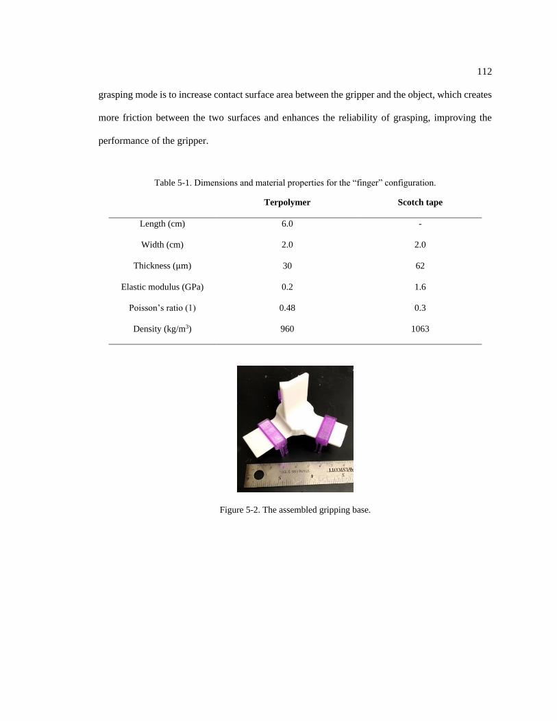
112

grasping mode is to increase contact surface area between the gripper and the object, which creates

more friction between the two surfaces and enhances the reliability of grasping, improving the

performance of the gripper.

Table 5-1. Dimensions and material properties for the “finger” configuration.

Terpolymer Scotch tape

Length (cm) 6.0 -

Width (cm) 2.0 2.0

Thickness (μm) 30 62

Elastic modulus (GPa) 0.2 1.6

Poisson’s ratio (1) 0.48 0.3

Density (kg/m3) 960 1063

Figure 5-2. The assembled gripping base.

113

Figure 5-3. Grasping experiments for several target objects including (a) a 60 mm pom-pom ball, (b) a

paper cylinder and (c) an inflated latex glove.

The design requirements are somewhat different between the two grasping modes due to

the different grasping mechanisms. For the enveloping mode, the actuation force is able to act

against the weight of the object as the actuator wraps fully around the object from bottom; therefore,

large free deflection of the terpolymer fingers is required in the enveloping mode. While in the

parallel mode, the actuation force mostly acts perpendicular to the weight of the object, in which

case the friction force between the actuator and the object is mainly responsible for holding the

object against gravity. Hence, terpolymer fingers with high blocked force are desirable when the

gripper works in the parallel mode. Therefore, to design a soft gripper capable of grasping multiple

types of objects will require optimizing both blocked force and free displacement. Quantitative

analysis and discussion of force and displacement of the finger actuator is presented next.

114

5.2.3 The Two-Stage Design Optimization Procedure

In this section, the proposed two-stage design optimization procedure is applied to realize

maximum actuation performance of the gripper device, and the corresponding flowchart is shown

in Figure 5-4 with specific design variables, objectives and outcomes of each stage defined in

Section 5.2.3.1.

Equivalently, the optimization is conducted for one finger of the gripper, which is modeled

as a segmented terpolymer-based unimorph actuator, as shown in Figure 5-5. As mentioned earlier,

both high free deflection and large blocked force are required for the gripper device to successfully

implement the two grasping modes. Hence, simultaneously maximizing the free deflection and the

blocked force are the design objectives in a multi-objective design problem. These two objectives

are competing, as the design with the highest free deflection will be very flexible and the design

with the highest blocked force will be very stiff. The two-stage optimization procedure is used to

resolve the tradeoff between the two objectives.

5.2.3.1 Stage 1

In Stage 1, computationally efficient analytical models are used to evaluate the objective

functions. The optimization results, i.e., the dimensions and locations of the active and passive

materials, are determined through Stage 1, and will remain fixed in Stage 2. In Stage 2, a full FEA-

based optimization is conducted to further improve the best design(s) from Stage 1 by introducing

non-uniform distributions of the active materials.

115

Figure 5-4. The flowchart of the two-stage optimization procedure for gripper design.

Figure 5-5. Schematic of the five-segment actuator.

The design optimization problem in Stage 1 is formulated in Equation 5-1. Since

optimization algorithms are developed to perform minimization, the design objectives in this study

are written equivalently to minimize the negative free deflection ∆𝑓𝑟𝑒𝑒 and negative blocked

force 𝐹𝑏, both at the tip of the finger. Based on investigation in Chapters 2 and 3, there are several

variables that may influence the two objectives, including the Young’s moduli and thickness of

both the terpolymer and the substrate, the total length of the actuator and the number of notches, as

well as their dimensions and positions along the actuator. In this study we consider an actuator with

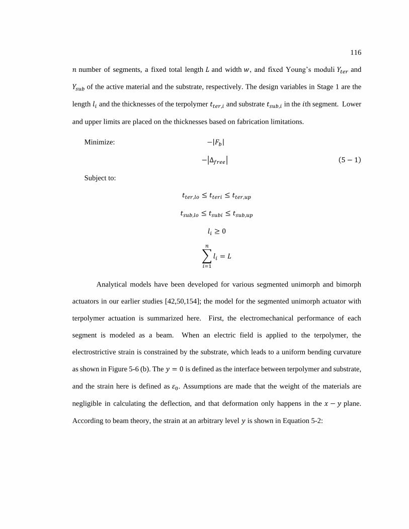
116

𝑛 number of segments, a fixed total length 𝐿 and width 𝑤, and fixed Young’s moduli 𝑌𝑡𝑒𝑟 and

𝑌𝑠𝑢𝑏 of the active material and the substrate, respectively. The design variables in Stage 1 are the

length 𝑙𝑖 and the thicknesses of the terpolymer 𝑡𝑡𝑒𝑟,𝑖 and substrate 𝑡𝑠𝑢𝑏,𝑖 in the 𝑖th segment. Lower

and upper limits are placed on the thicknesses based on fabrication limitations.

Minimize: −|𝐹𝑏|

−|∆𝑓𝑟𝑒𝑒| (5 − 1)

Subject to:

𝑡𝑡𝑒𝑟,𝑙𝑜 ≤ 𝑡𝑡𝑒𝑟𝑖 ≤ 𝑡𝑡𝑒𝑟,𝑢𝑝

𝑡𝑠𝑢𝑏,𝑙𝑜 ≤ 𝑡𝑠𝑢𝑏𝑖 ≤ 𝑡𝑠𝑢𝑏,𝑢𝑝

𝑙𝑖 ≥ 0

∑𝑙𝑖

𝑛

𝑖=1

= 𝐿

Analytical models have been developed for various segmented unimorph and bimorph

actuators in our earlier studies [42,50,154]; the model for the segmented unimorph actuator with

terpolymer actuation is summarized here. First, the electromechanical performance of each

segment is modeled as a beam. When an electric field is applied to the terpolymer, the

electrostrictive strain is constrained by the substrate, which leads to a uniform bending curvature

as shown in Figure 5-6 (b). The 𝑦 = 0 is defined as the interface between terpolymer and substrate,

and the strain here is defined as 휀0. Assumptions are made that the weight of the materials are

negligible in calculating the deflection, and that deformation only happens in the 𝑥 − 𝑦 plane.

According to beam theory, the strain at an arbitrary level 𝑦 is shown in Equation 5-2:

117

(a) (b)

(c)

Figure 5-6. The schematics of (a) the undeformed unimorph, (b) the deformed unimorph with bending

curvature 𝛋 and (c) two segments with their angular deflections.

휀𝑠𝑢𝑏(𝑦) = 휀0 + 𝑦𝜅 (−𝑡𝑠𝑢𝑏 ≤ 𝑦 ≤ 𝑡𝑡𝑒𝑟) (5 − 2)

For the substrate, the axial strain and stress due to bending (assuming linear material

behavior) are shown in Equations 5-3 and 5-4, respectively:

휀𝑠𝑢𝑏(𝑦) = 휀0 + 𝑦𝜅 (−𝑡𝑠𝑢𝑏 ≤ 𝑦 ≤ 0) (5 − 3)

𝜎𝑠𝑢𝑏(𝑦) = 𝑌𝑠𝑢𝑏 (휀0 + 𝑦𝜅) (−𝑡𝑠𝑢𝑏 ≤ 𝑦 ≤ 0) (5 − 4)

For the terpolymer, the total strain consists of the electrostrictive strain 휀𝑒and the induced

mechanical strain due to bending 휀𝑚. The expression of the mechanical strain is shown in Equation

5-5:

휀𝑚(𝑦) = 휀𝑡𝑜𝑡 − 휀𝑒 = 휀0 + 𝑦𝜅 − 𝑀𝐸2 (0 ≤ 𝑦 ≤ 𝑡𝑡𝑒𝑟) (5 − 5)

where 𝑀 is the electro-mechanical coupling coefficient and 𝐸 is the applied electric field.

When no external force and moment are applied on the actuator, the net resultant force is

shown in Equation 5-6:

118

∫ 𝜎𝑑𝐴 = 0

𝑡𝑡𝑒𝑟

−𝑡𝑠𝑢𝑏

⇒ ∫ 𝜎𝑠𝑢𝑏𝑑𝐴

0

−𝑡𝑠𝑢𝑏

+ ∫ 𝜎𝑚𝑑𝐴

𝑡𝑡𝑒𝑟

0

= 0 (5 − 6)

The net resultant moment is shown in Equation 5-7:

∫ 𝜎𝑦𝑑𝐴 = 0

𝑡𝑡𝑒𝑟

−𝑡𝑠𝑢𝑏

⇒ ∫ 𝜎𝑠𝑢𝑏𝑦𝑑𝐴

0

−𝑡𝑠𝑢𝑏

+ ∫ 𝜎𝑚𝑦𝑑𝐴

𝑡𝑡𝑒𝑟

0

= 0 (5 − 7)

The strain at the interface 휀0 and bending curvature are solved using these two equations

5-6 and 5-7. Extensions of this analytical model for a layered terpolymer actuator can be found in

[50].

According to the Bernoulli-Euler equation in Equation 5-8, the curvature is:

𝑀𝑒𝑞

𝑌𝐼=

𝑑𝜃

𝑑𝑠= 𝜅 (5 − 8)

The angular deflection 𝜃0 is shown in Equation 5-9:

∫ 𝑑𝜃

𝜃0

0

= ∫ 𝜅𝑑𝑠

𝑥2

𝑥1

𝜃0 = 𝜅𝑙 (5 − 9)

The tip displacements are shown in Equation 5-10:

𝛿𝑥 =1

𝜅(1 − 𝑐𝑜𝑠𝜅𝑙)

𝛿𝑦 = 𝑙 −𝑠𝑖𝑛𝜅𝑙

𝜅 (5 − 10)

The rotation angle 𝜃𝑖 for the 𝑖 th segment in the global coordinate system is given by

Equation 5-11:

𝜃𝑖 = 𝜃𝑙𝑜𝑐𝑎𝑙𝑖 + 𝜃𝑖−1 (5 − 11)

To calculate the free tip deflection of the segmented actuator, the tip displacement and

angular deflection of each segment are calculated first, and the accumulated tip displacement of

119

each segment is solved sequentially, as shown in Figure 5-6 (c). The accumulated tip displacement

in global coordinate system (𝑋𝑖 , 𝑌𝑖) is obtained by adding the contribution of the local displacement

(𝑋𝑡𝑖 , 𝑌𝑡𝑖) to the previous segment (𝑋𝑖−1, 𝑌𝑖−1), as shown in Equation 5-12:

[𝑋𝑖

𝑌𝑖] = [

𝑋𝑖−1

𝑌𝑖−1] + [

𝑋𝑡𝑖

𝑌𝑡𝑖] (5 − 12)

where:

[𝑋𝑡𝑖

𝑌𝑡𝑖] = [

𝑐𝑜𝑠𝜃𝑖−1 −𝑠𝑖𝑛𝜃𝑖−1

𝑠𝑖𝑛𝜃𝑖−1 𝑐𝑜𝑠𝜃𝑖−1] [

𝑥𝑖

𝑦𝑖] + [

𝑙𝑖𝑠𝑖𝑛𝜃𝑖−1

𝑙𝑖(1 − 𝑐𝑜𝑠𝜃𝑖−1)] (5 − 13)

The blocked force for a single unimorph segment has been derived in a previous study

[155]. In this section, the blocked force is derived for the segmented actuator with an arbitrary

number of segments, as shown in Figure 5-7 (a). An equivalent bending moment is applied at the

tip of each segment to account for the actuation from the terpolymer, and the blocked force is

modeled as an applied force at the tip of the entire actuator which results in a zero tip deflection.

According to Castigliano’s theorem as shown in Equation 5-14,

∆= ∑∫𝑀𝑖𝑛𝑡 (𝑥)𝜕𝑀𝑖𝑛𝑡 (𝑥)

𝜕𝐹𝑏

𝑑𝑥

𝑌𝐼𝑖

𝑛

𝑖=1

= 0 (5 − 14)

Based on equilibrium of bending moments, the internal moment in the 𝑖th segment 𝑀𝑖𝑛𝑡 is

derived from Equation 5-15:

𝑀𝑖𝑛𝑡 (𝑥) − ∑𝑀𝑒𝑞𝑖

𝑛

𝑖

+ 𝐹𝑏𝑥 = 0 (5 − 15)

where

∑𝑀𝑒𝑞𝑖

𝑛

𝑖

= (𝑌𝐼)𝑖𝜅𝑖 (5 − 16)

The blocked force is found by substituting Equations 5-15 and 5-16 into 5-14:

120

(a)

(b)

Figure 5-7. The schematics of (a) the equivalent bending moment and blocked force acting on an actuator

with 𝐧 segments and (b) the inner moment on the 𝐢th segment.

∑[(𝑙𝑖+1 + 𝑙𝑖+2 + ⋯+ 𝑙𝑛)2 − (𝑙𝑖 + 𝑙𝑖+1 + 𝑙𝑖+2 + ⋯+ 𝑙𝑛)2

2𝜅𝑖

𝑛

𝑖=1

+(𝑙𝑖 + 𝑙𝑖+1 + 𝑙𝑖+2 + ⋯+ 𝑙𝑛)3 − (𝑙𝑖+1 + 𝑙𝑖+2 + ⋯+ 𝑙𝑛)3

3

𝐹𝑏

𝑌𝐼𝑖] = 0 (5 − 17)

Given the geometric information for each segment, the segment bending curvature 𝜅𝑖 and

the segment bending stiffness 𝑌𝐼𝑖, the blocked force is found using Equation 5-17.

So far, the two design objectives, i.e., 𝐹𝑏 and ∆𝑓𝑟𝑒𝑒, for each design are obtained from the

analytical models and used in the optimizer NSGA-II for evolution. Once the Stage 1 optimization

is complete, the designer selects which design(s) to move forward to Stage 2. A single design can

be selected based on particular requirements. For the gripper application, we seek a design with

both suitable free deflection and blocked force and select one design out of the set of non-dominated

121

designs. As introduced in Section 4.2.1, the distance measure is an effective approach to select the

overall best design. A general multi-objective distance measure is expressed as in Equation 4-1.

Here, the power term 𝑝 is selected as 2, the weights 𝑐1 = 𝑐2 = 0.5 since 𝐹𝑏 and ∆𝑓𝑟𝑒𝑒 are

considered equally important, and the ideal values for the design objectives are decided later in

Section 5.2.4. So the distance measure is expressed as in Equation 5-18:

𝑈 = √[0.5(𝐹𝑏(𝑥)

𝐹𝑏0 − 1)]2 + [0.5(

∆𝑓𝑟𝑒𝑒(𝑥)

∆𝑓𝑟𝑒𝑒0 − 1)]2 (5 − 18)

The design with the minimum distance measure is thus selected to move forward to Stage 2.

5.2.3.2 Stage 2

The outcome of Stage 1 consists of the lengths and the thicknesses of the terpolymer and

the substrate of each segment, which are then held fixed as inputs in Stage 2. One of the assumptions

in Stage 1 is that the width 𝑤 is a constant for all segments, which enables use of computationally

less expensive 2-D analytical models.

In Stage 2, 3-D FEA models are developed to evaluate the objective functions, providing

the opportunity to investigate other design variables, such as non-uniform distribution of the active

materials. In this section, considering the actuation mechanism of the terpolymer, the shapes of

each segment are adopted as the design variables. In Stage 2, variation in width of each segment is

introduced which allows the surfaces of the segments to be rectangular or trapezoidal. The edge

slopes 𝑆𝑙𝑜𝑝𝑒𝑖 for each segment are adopted as the design variables in Stage 2, as shown in Figure

5-8. Thus, the design variables are the edge slope of each segment, while the design objectives

remain the same as in Stage 1 but are calculated using the 3D FEA simulation. The design

optimization problem is formulated as in Equation 5-19:

Minimize: −|𝐹𝑏|

122

−|∆𝑓𝑟𝑒𝑒|

Subject to:

𝐹𝑜𝑟 𝑖 𝑓𝑟𝑜𝑚 1 𝑡𝑜 𝑛 (5 − 19)

𝑆𝑙𝑜𝑝𝑒𝑙𝑜 ≤ 𝑆𝑙𝑜𝑝𝑒𝑖 ≤ 𝑆𝑙𝑜𝑝𝑒𝑢𝑝

𝑤𝑖𝑡ℎ 𝑙𝑖 , 𝑡𝑡𝑒𝑟𝑖 , 𝑎𝑛𝑑 𝑡𝑠𝑢𝑏𝑖 𝑑𝑒𝑡𝑒𝑟𝑚𝑖𝑛𝑒𝑑 𝑓𝑟𝑜𝑚 𝑠𝑡𝑎𝑔𝑒 𝑜𝑛𝑒.

The FEA model follows the same method as is introduced in Chapter 3, where the

constitutive relations of the electrostrictive terpolymer are developed and then implemented in the

shell module of the commercial FEA package COMSOL Multiphysics. The FEA models for free

deflection are validated in Chapter 3.

Figure 5-8. The trapezoid shape of surface of the 𝐢th segment with edge slope 𝑺𝒍𝒐𝒑𝒆𝒊. The area of the

surface and accordingly the volume of the materials remain the same from Stage 1 to Stage 2.

Besides the free deflection, the FEA models are implemented to predict the blocked forces

generated by the terpolymer-based actuators. The 3 cm-long unimorph bender is used as the

validation configuration since corresponding experimental measurements have been conducted for

the blocked forces by Saad Ahmed et al. [50]. To improve the blocked force, multiple layers of the

terpolymer are adhered together using spray glue. In the FEA model, a roller boundary condition

is assigned to the tip of the bender by prescribing the tip-displacement in the x- direction to be zero,

as depicted in Figure 5-9; the bender is free to move in the y-z plane. The multiple layers of

123

terpolymer is modeled in FEA in such a way that a glue layer with thickness 𝑡𝑔 and elastic modulus

𝑌𝑔 is used between two terpolymer layers. Through a parametric study, the parameters of the glue

layer are determined as 𝑡𝑔 = 2𝜇𝑚 and 𝑌𝑔 = 750 𝑀𝑃𝑎.

Quantitative comparisons of the blocked force between FEA and experiments are shown

in Figure 5-10, where the bender is actuated using 1 layer, 4 layers, and 6 layers of the terpolymer,

respectively. The error bars represent plus/minus one standard deviation of five samples in each

case. We can see that FEA results agree well with experimental data for all of the three cases

especially at high electric field 50 MV/m when the error bars are considered. As the number of

layers of the terpolymer increases, the blocked force also increases evidently. The actuators with

four and six terpolymer layers generate blocked forces approximately four times higher and seven

times higher than the single layer actuator, respectively. Through this study, the FEA models to

predict the blocked force generated by multilayer terpolymer-based actuators are validated.

Figure 5-9. Roller boundary condition is assigned at the bottom edge of the unimorph bender to compute

the blocked force.

124

Figure 5-10. Blocked force comparison between FEA and experiments for the unimorph bender.

After validation, the FEA models are then used in Stage 2. A sample FEA model with

trapezoidal segments is presented in Figure 5-11. A symmetric boundary condition is applied at the

center line of the structure to reduce computational cost, taking advantage of the symmetric

geometry. The mesh is generated using COMSOL mesh controller, where triangular mesh

geometry and “normal” extent of fineness are selected.

NSGA-II is applied as the optimization algorithm and is implemented using MATLAB’s

gamultiobj function [156]. MATLAB and COMSOL interact such that MATLAB generates the

values of the design variables and sends them to a COMSOL model file. COMSOL generates the

geometry based on these variable values in a FEA model and evaluates the corresponding

objectives ∆𝑓𝑟𝑒𝑒 and 𝐹𝑏, and then sends the objective values back to MATLAB for optimization,

which sends them to COMSOL again. The process is repeated until convergence is achieved.

Through Stage 2, all the designs appearing on the Pareto front of the final generation

represent the best designs in the two objective functions. The designer may select the final design

based on particular application requirements, or by using the distance measure as in Stage 1. Note

that in general, the utopia point in Stage 2 is different from that in Stage 1.

125

Figure 5-11. The meshed FEA model with trapezoid segment surfaces where 𝑺𝒍𝒐𝒑𝒆𝒊 = 𝟎. 𝟏𝟐. A symmetric

boundary condition is applied along the center line considering the symmetric geometry of the actuator.

5.2.4 Results

5.2.3.2 Results of Stage 1

The two-stage design optimization procedure is applied to the double notched “finger”

configuration, which is modeled as a five-segment unimorph actuator (𝑛 = 5), as shown in Figure

5-5. The optimization problem is formulated as shown in Equation 5-1. According to fabrication

limitations, the upper and lower bounds of the terpolymer are set as 𝑡𝑡𝑒𝑟,𝑙𝑜 = 30 𝜇𝑚 and 𝑡𝑡𝑒𝑟,𝑢𝑝 =

300 𝜇𝑚 respectively, and similarly for the substrate, 𝑡𝑠𝑢𝑏,𝑙𝑜 = 40 𝜇𝑚, and 𝑡𝑠𝑢𝑏,𝑢𝑝 = 400 𝜇𝑚. The

free deflection and blocked force are calculated at 𝐸 = 40 𝑀𝑉/𝑚 , and the coefficient 𝑀 =

4.38 × 10−18𝑚2/𝑉2 in Equation 5-5.

There are 14 design variables in Stage 1: the length of each segment 𝑙1, 𝑙2, 𝑙3, 𝑙4 (𝑙5 is

determined thereafter since the total length 𝐿 is fixed), the thicknesses of the terpolymer in each

segment 𝑡𝑡𝑒𝑟1, 𝑡𝑡𝑒𝑟2 …𝑡𝑡𝑒𝑟5 , and thicknesses of the substrate 𝑡𝑠𝑢𝑏1, 𝑡𝑠𝑢𝑏2 …𝑡𝑠𝑢𝑏5 . Based on the

number of design variables of 14, the recommended population size from MATLAB 𝑁𝑝 = 200 is

adopted. The stopping criterion is defined as when the average spread change evaluted for the latest

126

100 generations is smaller than the function tolerance of 10−4. Several algorithm parameters have

been tuned to achieve good diversity in the population and convergence within a reasonable time.

The Pareto fraction is set as 0.7, the elite fraction is 0.05, the crossover fraction is 0.5, and the

mutation option is “Mutationadaptfeasible”, in which the mutation direction and step length are

calculated based on the variable bounds and linear constraints. The CPU time for convergence is

about 130 seconds, going through over 150 generations of evolution.

The performance space of the final generation of Stage 1 is presented in Figure 5-12, where

the horizontal axis is the negative normalized free deflection ∆𝑓𝑟𝑒𝑒, and the vertical axis is the

negative normalized blocked force 𝐹𝑏 at an applied electric field 𝐸 = 40𝑀𝑉/𝑚. ∆𝑓𝑟𝑒𝑒 and 𝐹𝑏 are

normalized with respect to the best individual values that are achieved in the final generation, which

are later used as the utopia point in the calculation of the distance measure. Since the design

objectives are to maximize both ∆𝑓𝑟𝑒𝑒 and 𝐹𝑏, the ideal design would be located near the origin

(bottom left corner) of the performance space. In the plot, each point represents a Pareto optimal

design. The total number of designs appearing in the Pareto front is 𝑁𝑝𝑎𝑟𝑒𝑡𝑜 = 𝑁𝑝 ×

𝑃𝑎𝑟𝑒𝑡𝑜𝐹𝑟𝑎𝑐𝑡𝑖𝑜𝑛 = 200 × 0.7 = 140.

The parameters used in the calculation of the distance measure (see Equation 5-18) are

determined as follows. By observing the performance space, the best possible value of the blocked

force is defined as 𝐹𝑏0 = 71 𝑚𝑁, and the best value of the free deflection is defined as ∆𝑓𝑟𝑒𝑒

0 = 9 𝑐𝑚

for calculation of the distance measure. The power term 𝑝 is selected as 2, and the two objectives

are treated with equal importance, i.e.,, 𝑐1 = 𝑐2 = 0.5, so that the distance measure represents the

distance of a specified design to the utopia point.

The distance measures of all 140 designs in the Pareto front are evaluated, and the design

with the minimum distance measure is noted in Figure 5-12, and is depicted in Figure 5-13 (a),

where the lengths and thicknesses of the segments are shown approximately to scale. The values

127

of the design variables are listed in Table 5-2. This design can generate ∆𝑓𝑟𝑒𝑒= 3.51𝑐𝑚 and 𝐹𝑏 =

43.7 𝑚𝑁 when the applied field 𝐸 = 40 𝑀𝑉/𝑚, resulting in a distance measure 𝑈 = 0.361. It is

observed that this best design exhibits a nearly tapered configuration, with relatively thicker

terpolymer and substrate layers in the segments near the root and thinner layers in the segments

near the tip. Moreover, the very top and very bottom segments are longer than the other three

segments. The notches do not appear in the best design, since the blocked force 𝐹𝑏 is considered

besides the free deflection ∆𝑓𝑟𝑒𝑒. Further analysis is presented in Section 5.2.5.

To demonstrate the advantage of the segmented structure and the improvement achieved

through Stage 1, the best design in Stage 1 is compared to a standard unimorph, which is a non-

segmented structure with uniform terpolymer thickness of 279 𝜇𝑚 and substrate thickness of

160 𝜇𝑚. The material thicknesses of the standard unimorph is selected such that the volumes of

the terpolymer and the substrate are the same as the total corresponding material volumes of the

best design, respectively. The performance of the standard unimorph is shown in Figure 5-12, and

a performance comparison can be seen in Table 5-3. Note that the selected best design in Stage 1

exhibits higher 𝐹𝑏 but lower ∆𝑓𝑟𝑒𝑒 than the standard unimorph, but has a lower distance measure,

representing an improvement in overall performance.

As can be seen in Figure 5-12, there are optimal designs with better performance in both

∆𝑓𝑟𝑒𝑒 and 𝐹𝑏 than the standard unimorph, demonstrating the effect of the optimization. To illustrate

this point, two designs, namely Design 1 and Design 2, are selected and compared to the standard

unimorph, where Design 1 exhibits the same 𝑭𝒃 but higher ∆𝒇𝒓𝒆𝒆 than the standard unimorph,

while Design 2 shows the same ∆𝒇𝒓𝒆𝒆 but higher 𝑭𝒃 . These two designs exhibit better overall

performance than the standard unimorph but worse than the best design when evaluated using the

distance measure as expressed in Equation 5-18. However, we can see from Table 5-3 that the

volumes of terpolymer material used in Design 1 and Design 2 are less than either the standard

128

unimorph or the best design. If the volume of terpolymer material 𝑉𝑡𝑒𝑟 is introduced into the

distance measure as a third metric besides ∆𝒇𝒓𝒆𝒆 and 𝑭𝒃, and the weights of these three metrics are

reassigned, we may have the best design different from current one, which reveals that the criteria

to determine the best design is decided by the designer and is not unique, and metrics beyond the

design objectives can be included in the calculation of the distance measure, for example, the

volume of terpolymer used in the gripper.

Figure 5-12. The performance space of the standard unimorph and the final generation from Stage 1. The

position of the best design in Stage 1 is determined by the minimum value of distance measure.

(a) (b)

Figure 5-13. Schematics of (a) the best design from Stage 1, showing a nearly tapered configuration

along the length, and (b) a standard unimorph. The thicknesses are exaggerated compared to lengths.

129

Table 5-2. The values of the design variables for the best design in Stage 1.

Variable name value Variable name value

𝑙1 2.607 𝑐𝑚 𝑡𝑡𝑒𝑟4 278 𝜇𝑚

𝑙2 1.039 𝑐𝑚 𝑡𝑡𝑒𝑟5 242 𝜇𝑚

𝑙3 0.183 𝑐𝑚 𝑡𝑠𝑢𝑏1 209 𝜇𝑚

𝑙4 0.605 𝑐𝑚 𝑡𝑠𝑢𝑏2 152 𝜇𝑚

𝑡𝑡𝑒𝑟1 298 𝜇𝑚 𝑡𝑠𝑢𝑏3 180 𝜇𝑚

𝑡𝑡𝑒𝑟2 291 𝜇𝑚 𝑡𝑠𝑢𝑏4 107 𝜇𝑚

𝑡𝑡𝑒𝑟3 275 𝜇𝑚 𝑡𝑠𝑢𝑏5 100 𝜇𝑚

Table 5-3. Performance comparison between the standard unimorph and the best design in Stage 1.

Design ∆𝒇𝒓𝒆𝒆(cm) 𝑭𝒃 (mN) distance

measure 𝑽𝒕𝒆𝒓 (cm3)

Standard unimorph 3.87 35.2 0.381 0.168

Design 1 4.14 35.2 0.368 0.155

Design 2 3.87 39.1 0.371 0.160

Best design in stage one 3.51 43.7 0.361 0.168

5.2.3.2 Results of Stage 2

In Stage 2, the initial dimensions of the design are determined from Stage 1 as listed in

Table 5-2, and the design variables are the edge slopes 𝑆𝑙𝑜𝑝𝑒𝑖 of each segment. The design

optimization problem is formulated as shown in Equation 5-19, where the bounds of 𝑆𝑙𝑜𝑝𝑒𝑖 are set

as −0.125 ≤ 𝑆𝑙𝑜𝑝𝑒𝑖 ≤ 0.125 to guarantee that the lengths of the top and bottom edges of all

segments are always positive.

Computation time is an important consideration in design optimization. Based on our

previous experience, it takes each FEA simulation about one hour to obtain both ∆𝑓𝑟𝑒𝑒 and 𝐹𝑏 for

130

a single design when the applied field 𝐸 = 40 𝑀𝑉/𝑚, thus making the FEA-based optimization

computationally expensive. To reduce computation time, we propose to run the Stage 2 FEA

simulations for electric field 𝐸 = 1 𝑀𝑉/𝑚 to avoid the high nonlinearity in deformation and the

large number of iterations for the FEA model to converge. Since ∆𝑓𝑟𝑒𝑒 and 𝐹𝑏 increase nonlinearly

with the electric field, we cannot just extrapolate the performance at higher fields. Here the question

is: are the best designs at 𝐸 = 1 𝑀𝑉/𝑚 still the best designs at 𝐸 = 40 𝑀𝑉/𝑚?

To answer this question, 15 designs on the Pareto front in the parametric study of [128] are

selected to compare their performance at 𝐸 = 1 𝑀𝑉/𝑚 and 𝐸 = 40 𝑀𝑉/𝑚. The results are shown

in Figure 5-14. It is observed that the relative positions on the Pareto front of the selected 15 designs

for 𝐸 = 40 𝑀𝑉/𝑚 and 𝐸 = 1 𝑀𝑉/𝑚 remain the same, indicating that the best designs for 𝐸 =

40 𝑀𝑉/𝑚 still surpass other designs in both design objectives for 𝐸 = 1 𝑀𝑉/𝑚 . The result

validates the feasibility of implementing the FEA-based optimization for 𝐸 = 1 𝑀𝑉/𝑚 to save

computation time. Even with this simplification, it takes the FEA simulation about 5 minutes to

converge for a single design. The population size is set as 𝑁𝑝 = 50, and the algorithm stops when

the convergence criterion is reached, which will be explained later. The total computing time in

Stage 2 is 360 hours (15 days).

(a) (b)

Figure 5-14. The positions of the 15 selected designs in (a) performance space of the parametric design

when 𝐸 = 40 𝑀𝑉/𝑚 and (b) when 𝐸 = 1 𝑀𝑉/𝑚 .

131

The performance space of the entire inital generation, the Pareto front of the 108th

generation, along with the Stage 1 best design, are shown in Figure 5-15 (a). The best designs in

the 108th generation can be seen more clearly in Figure 5-15 (b), where the horizontal axis is the

negative normalized free deflection and the vertical axis is the negative normalized blocked force

when the applied field is 𝐸 = 1 𝑀𝑉/𝑚. It is observed that the design performance is notably

improved from initial generation to the 108th generation. Note that all the designs on the Pareto

front perform better than the best design in Stage 1, indicating the improvement achieved through

Stage 2. Again, the distance measure is applied to evaluate the overall performance of these designs.

In Stage 2, ∆𝑓𝑟𝑒𝑒0= 0.0165𝑐𝑚 and 𝐹𝑏

0 = 0.219 𝑚𝑁 are adopted as the utopia values. The design

with the minimum distance measure is noted in Figure 15 (b).

The trend of the spreadchange value in the last 11 generations is shown in Figure 5-16. The

spread is a measure of the movement of the Pareto set [156], and the spreadchange is calculated as

the difference between the current generation and the average of the latest certain number of

generations, called stall generations. As convention, the spreadchange value is adopted as the

convergence criterion to reflect relative change between generations. Based on our previous

experience on multi-objective FEA-based optimization [157], the value of stall is selected as 5. As

we can see in Figure 5-16, the spreadchange value drops from 0.025 to 0.0025 from generation 98

to 108, indicating that the optimization algorithm can be considered converged at the 108th

generation.

By checking the performance of the designs with assistance of the performance space, the

designer may select the final design based on particular application requirements, or by using the

distance measure as in Stage 1. A schematic of the design with best distance measure in Stage 2 is

depicted in Figure 5-17, where the edge slopes 𝑆𝑙𝑜𝑝𝑒𝑖 are listed in Table 5-4. According to the

132

FEA model, this design can generate ∆𝑓𝑟𝑒𝑒= 0.0164𝑐𝑚 and 𝐹𝑏 = 0.219 𝑚𝑁 when the applied

field 𝐸 = 1 𝑀𝑉/𝑚, resulting in a distance measure 𝑈 = 0.00185. It can be seen that in this design,

the width first decreases and then increases in both the root half and the tip half.

(a)

(b)

Figure 5-15. (a) The performance space of the best design in Stage 1, the initial generation and pareto front

of the 51st generation in Stage 2. (b) a zoomed plot of the designs in the 51st generation.

133

Figure 5-16. The trend of spreadchange value in the last 11 generations where the algorithm tends to

converge.

terpolymer substrate

Figure 5-17. Schematic of the best design generated from Stage 2, where the thicknesses are exaggerated

compared to lengths.

Design performance at 𝐸 = 40 𝑀𝑉/𝑚 is compared among the standard unimorph, the best

design in Stage 1 and the best design in Stage 2, as shown in Table 5-5, where the FEA model is

used to evaluate ∆𝑓𝑟𝑒𝑒 and 𝐹𝑏 , and the improvements in percentage are based on the standard

unimorph. To be consistent with Stage 1 and to include the geometric nonlinearity, the designs are

evaluated at electric field 𝐸 = 40 𝑀𝑉/𝑚. Compared to the standard unimorph, the Stage 1 best

134

design exhibits a large improvement in blocked force (20.6%) for a small decrease in free deflection

(8.7%). The Stage 2 best design exhibits further improvement in blocked force (29.9%) without

sacrificing any free deflection compared to the Stage 1 best design. It should be emphasized that

all three designs use the same amount of active and passive material. The simualted deformed

shapes of these three designs in both free deflection and blocked force conditions are shown in

Figure 5-18.

Table 5-4. The values of the design variables for the best design in Stage 2

Variable name value

𝑆1 0.0568

𝑆2 -0.0395

𝑆3 -0.0114

𝑆4 0.0180

𝑆5 -0.0396

Table 5-5. Performance comparison among the standard unimorph, the best design in stage one and the best

design in Stage 2 based on the FEA model when 𝑬 = 𝟒𝟎 𝑴𝑽/𝒎.

∆𝑓𝑟𝑒𝑒(cm) 𝐹𝑏 (mN)

Standard unimorph 4.84 48.5

Stage 1 best design 4.42 (8.7% ↑) 58.5 (20.6% ↑)

Stage 2 best design 4.42 63.0 (29.9% ↑)

135

(a) standard unimorph free deflection (b) standard unimorph blocked

(c) best design in Stage 1 free deflection (d) best design in Stage 1 blocked

(e) best design in Stage 2 free deflection (f) best design in Stage 2 blocked

Figure 5-18. The simulated deformed shapes of the standard unimorph and best designs in Stage 1 and in

Stage 2 under free deflection and blocked conditions.

136

5.2.5 Discussion

In this section, the proposed computationally efficient two-stage design optimization

procedure is successfully applied to determine the best design for a soft gripper, which is actuated

using the electrostrictive PVDF-based terpolymer. NSGA-II is adopted as the optimization

algorithm for its capacity to deal with multi-objective optimization problems and to find the global

optima with a good amount of design variables and large design space. In Stage 1, the

computationally less expensive analytical models are developed based on Bernoulli-Euler beam

theory and Castigliano’s theorem to calculate ∆𝑓𝑟𝑒𝑒 and 𝐹𝑏. Segment lengths and thicknesses of the

terpolymer and the substrate for each segment are defined as the design variables, with upper and

lower bounds according to fabrication limitations. In Stage 2, 3-D FEA models are developed using

the dimensions that are determined by the best design in Stage 1 to investigate effects of the shape

of segment surfaces. The edge slopes in each segment are opmized to further improve the designs.

Compared to an optimization procedure using a full FEA-based optimization, this two-

stage design is more computationally efficient by employing 2-D analytical models in Stage 1

where assumptions are made to reduce the degrees of freedom, and thus reducing the parameter

space in Stage 2 where FEA comes in. In the finger example, 14 design variables are investigated

in Stage 1 to determine the dimensions of the segmented actuator. A relatively large population

size 𝑁𝑝 = 200 is adopted in the optimization algorithm, and it undergoes 150 generations to

converge. As a result, it takes 200 × 150 = 30,000 runs to determine the best design in Stage 1,

while the entire computation lasts only about 130 seconds. If Stage 1 were conducted using a full

FEA-based optimization, considering that it takes 5 minutes to complete computation for one

design, it would take 30,000 × 5 𝑚𝑖𝑛𝑢𝑡𝑒𝑠 = 150,000 𝑚𝑖𝑛𝑢𝑡𝑒𝑠 = 104 𝑑𝑎𝑦𝑠 to complete the

optimization. The analytical model-based optimization in Stage 1 is necessary to make the

computation tractable.

137

Although the modeling method applied in Stage 1 is computationally efficient, it does not

account for 3-D behavior or nonuniform distribution of active materials. For that reason, Stage 2

utilizes 3-D FEA models since they can directly account for the electro-mechanical coupling

effects, non-uniform spatial distribution of the active materials, 3-D behavior, and the influence of

abrupt changes in geometry or material properties that lead to highly localized deformation. It is

recommended that a relatively small number of design variables is favored in the FEA-based

optimization in Stage 2.

The trade-off between model accuracy and computational efficiency is illustrated by

comparing the analytical model used in Stage 1 and the FEA model used in Stage 2, as presented

in Figure 5-19. Here, the computational efficiency is represented by the inverse of CPU time in

seconds. For model accuracy, free deflection ∆𝑓𝑟𝑒𝑒 is used as the metric; the model accuracy is

defined as the ratio of the analytical model results and the FEA resutls, and model accuracy is set

to 1 for the FEA model, since the FEA models have been validated with experiments. We can see

from Figure 5-19 that as the fidelity, namely, the degrees of freedom, of the model increases, the

model accuracy also increases; however, the sacrifice in the computational efficiency is notable.

This further demonstrates the effectiveness of the two-stage approach that by losing some fidelity

in Stage 1, the computational efficiency is largely enhanced and the total computational cost of

design optimization is reduced. This trend remains as the structures and the corresponding models

become more complex.

138

Figure 5-19. The trade-off between model accuracy and computational efficiency is presented by

comparing the analytical model and FEA model.

To effectively reduce computational cost, geometric complexity should be accounted for

in the low-fidelity model as much as possible. For example, in the gripper design, if there exists a

validated low-fidelity analytical model to calculate ∆𝑓𝑟𝑒𝑒 and 𝐹𝑏 with a trapezoid surface geometry

as described in Stage 2, then this analytical model should be used in the optimization process; in

this case, Stage 2 is no longer needed. Similarly, if an analytical model is developed to account for

nonuniform thicknesses of terpolymer and the substrate, for example, thicknesses of polynomial

expressions, then a spline could be used to connect the five segments, which may provide higher

resolution in the results and reveal more insights of the influences of the design variables.

There are several things that we can learn from the optimization results. The best design

from Stage 1 exhibits a nearly tapered configuration, as shown in Figure 5-13. Thicker terpolymer

and substrate layers are observed in the segments close to the root, while thinner layers appear in

the segments close to the tip, which indicates that the segments close to the root exert greater

influence on the blocked force and conversely the segments close to the tip play a more important

role in enhancing free deflection. Moreover, the segments very close to either the root or the tip are

139

notably longer than the segments in between, indicating that the tip and root regions dominate in

the actuation performance and the transition between them is relatively short.

The best design from Stage 2 demonstrates that the actuation performance is further

improved from Stage 1 by adjusting the shape of the segment surface. Without sacrificing any free

deflection, the blocked force is further improved by 30% in Stage 2. Good convergence is observed

in the last 11 generations.

5.3 Design of an Origami-inspired Multifield “Coffee Table”

5.3.1 Introduction

To demonstrate the applicability of the proposed two-stage design optimization procedure

to multifield responsive structures, an origami-inspired “coffee table” configuration is optimized,

where both electroactive terpolymer and the MAE are used to realize multifield actuation. This

configuration has been applied in real life for furniture, as shown in Figure 5-19. In this section,

this “coffee table” configuration is modified as shown in Figure 5-20 (c) and then used as a case

study for demonstration of the two-stage optimization since achieving folds at different locations

is an appropriate case for multifield actuation. The electrostrictive terpolymer and the MAE have

been demonstrated as applicable actuation mechanisms for self-folding configurations in chapters

2 and 3, and are also used to achieve the target shape shown in Figure 5-20 (c). Here, the folds in

the middle of the “coffee table” and the four corners are decomposed and actuated using the MAE

and terpolymer respectively, with corresponding target shapes shown in Figure 5-20 (a) and (b).

140

Figure 5-20. A real origami-inspired coffee table [158].

The objectives in the design of the “coffee table” are to minimize the shape error between

the simulation and the target shape, as defined in Section 4.3.1, and also to minimize the total

volume of the active materials. The two-stage design optimization procedure is implemented,

wherein Stage 1 a computational inexpensive rigid body dynamic model is used as the low-fidelity

model to evaluate design performance because there are validated rigid body dynamic models to

simulate the actuations of the MAE and terpolymer, and the best design is selected as the baseline

design in Stage 2; while in Stage 2 FEA models are used to further improve the designs. A

flowchart for the two-stage design optimization procedure where rigid body models are used in

Stage 1 is described in Figure 4-2, and it is slightly simplified based on the “coffee table” design

in this section. More details in the problem formulation and optimization results are presented in

the following sections.

5.3.2 The Two-Stage Design Optimization Procedure

5.3.2.1 Stage 1

A specific flowchart of Stage 1 for the “coffee table” design is presented in Figure 5-21, in

which the actions in each step, design variables, design objectives and optimizer are specified and

are defined later in this section.

141

Figure 5-21. Schematics of the target shapes for the “coffee table” upon application of magnetic field (a),

electric field (b)and both fields simultaneously(c).

Figure 5-22. The flowchart of Stage 1 for the “coffee table” design.

142

To determine the crease pattern of the base structure, a software called “origami pattern

designer” is used, which was developed by our collaborators Xi and Lien [18]. In the software, two

types of creases, namely, mountain creases and valley creases, can be created based on the direction

of fold, as depicted in Figure 5-22. According to the final deformed target shape of the “coffee

table”, the crease pattern is created on the initially flat base structure, as shown in Figure 5-23 (a),

where the red creases represent mountain creases, the blue ones represent valley creases while the

gray ones are auxiliary creases to facilitate folds in the software. Folding angles are assigned to

each crease to a achieve the target shape shown in Figure 5-20 (c). Here, the folding angles at the

four corners, on the two long mountain creases and on the middle valley crease are 90°, 45° and

90° , respectively, measured between the two adjacent panels connected by that creaase. The

deformed shape in the software is shown in Figure 5-23 (b).

Figure 5-23. A crease can be folded as either a mountain fold (in red) or a valley fold (in blue) in the

software “origami pattern designer” [18].

As stated in Chapter 4, the applicability of rigid body dynamic models to self-folding

structures has been demonstrated. In this section, a rigid body dynamic model is developed in the

Multibody Dynamics module of the commercial FEA software package COMSOL Multiphysics.

A schematic of the rigid body dynamic model is depicted in Figure 5-25. The base structure is

divided into eight subdomains, each of which is modeled as a rigid panel. Every pair of two adjacent

panels are connected by a one-degree-of-freedom hinge joint, where rotation is allowed in only one

143

direction. Panel 3 in yellow is fixed in the reference spatial frame. To fold the four corners, torques

representing the actuation of the terpolymer, denoted as 𝑇𝐸 and referred to as “electric torques”, are

applied on the four corner creases. Torques representing the actuation of the MAE, denoted as 𝑇𝑀

and referred to as “magnetic torques”, are applied on the three blue panels where the MAE patches

are attached.

(a) (b)

Figure 5-24. (a) The crease pattern of the “coffee table” designed in the software “origami pattern

designer”, where the red creases represent mountain creases, while the blue ones represent valley creases.

(b) The deformed shape with corresponding folding angles.

Figure 5-25. Schematic of the rigid body dynamic model of the “coffee table”.

144

The selection of design variables is described here. As introduced in Section 4.3, the

potential design variables are the external torques 𝑇 that can be applied to the rigid panels in 𝑥, 𝑦

and 𝑧 directions, and the torsional spring constants 𝐾 on the hinge joint. However, in this design

problem, one objective is to minimize the total torque magnitude 𝑇𝑡𝑜𝑡 needed. According to

Equation 4-3, to achieve a particular folding angle, the required torque is proportional to the

torsional spring constant. Intuitively, to reduce 𝑇𝑡𝑜𝑡, low spring constants 𝐾 should be used. The

torsional springs represent the bending stiffness of the crease material; so, a compliant material

PDMS is assumed as the crease material to connect the three blue magnetic panels, and the

corresponding spring constants 𝐾 are determined, as shown in Table 5-6. Therefore, in Stage 1 of

this design problem, the only design variables are the torques 𝑇𝐸 and 𝑇𝑀. The next action is to apply

the variable filter. As described in Section 4.3, to meet kinematic compatibility, the resultant torque

on each panel should align with its rotation direction. Therefore, instead of torques applied in 𝑥, 𝑦

and 𝑧 directions, the magnetic torques are applied only in the 𝑦 direction, and the resultant electric

torques are applied along the corresponding crease directions. To reduce number of design

variables, an assumption is made, based on the symmetry of the structure between the upper and

lower halves, that the electric torques are the same on Creases 1 and 7, denoted as 𝑇𝐸1, and the

same on Creases 2 and 8, denoted as 𝑇𝐸2. To summarize, there are five design variables in Stage 1,

including three magnetic torques and two electric torques.

The dimensions and material properties are listed in Table 5-6. The unit panel length 𝐿𝑝 is

1 cm. To determine the torsional spring constants 𝐾 using the SLFP model introduced in Section

4.3, the width of the creases connecting magnetic panels (referred to as “magnetic creases” in the

rest of the chapter) 𝑤𝑐𝑀 is selected as 0.2Lp (0.2cm), while the width of the four corner creases

(referred to as “electric creases” in the rest of the chapter) is selected as 0.3Lp (0.3cm) to achieve

sufficient folding angles. The positions of these creases are denoted in Figure 5-25.

145

Table 5-6. The dimensions, material properties and corresponding torsional spring constants in Stage 1.

parameter value parameter value

𝐿𝑝 1 cm 𝐾𝐸,1 2.81× 10−7 Nm/°

𝑌𝑐𝐸 0.02 GPa 𝐾𝐸,2 𝐾𝐸,1

𝑌𝑡𝑒𝑟 0.2 GPa 𝐾𝑀,1 8.33 × 10−7 Nm/°

𝑡𝑐𝐸 15 μm 𝐾𝑀,2 𝐾𝑀,1

𝑡𝑡𝑒𝑟 20 μm 𝐾𝑀,3 𝐾𝑀,1

𝑤𝑐𝐸 0.3 Lp 𝑇𝑙𝑜𝑤 0

𝑌𝑐𝑀 0.5 MPa (PDMS) 𝑇𝑢𝑝𝑝𝑒𝑟 π ∙ 𝐾

𝑡𝑐𝑀 100 μm

𝑤𝑐𝑀 0.2 Lp

Figure 5-26. The positions of the magnetic and electric creases.

In order to achieve target shape consisting of folding angles of 90° for terpolymer actuation

at the four corners, the analytical models developed in Section 5.2 are used to determine appropriate

dimensions and material properties in the electric creases. As a result, the elastic modulus of the

substrate material 𝑌𝑐𝐸 is selected as 0.02 GPa, and the thicknesses of the substrate and terpolymer

are determined as 15 𝜇𝑚 and 20 𝜇𝑚, respectively.

146

Based on the material properties and dimensions discussed above, the effective torsional

spring constants in the creases are calculated using Equation 4-2, and the values are listed in Table

5-6.

To avoid self-intersection of the panels, which leads to divergence of the FEA model,

kinematic constraints are applied with the corresponding strategy expressed as in Equations 5-20:

0 < 𝜃𝑘 < 𝜃𝑘,0 + Δ𝜃 (5 − 20)

where 𝜃𝑘 and 𝜃𝑘,0 are the folding angles of the 𝑘th crease in simulation and in the target shape,

respectively, and Δ𝜃 determines how much 𝜃𝑘 can possibly go beyond 𝜃𝑘,0. According to the 𝜃𝑘

and geometry of the “coffee table”, Δ𝜃 = 𝜋4⁄ is selected, and the specific inequalities for

kinematic constraints are expressed in Equation 5-24, which is derived later in this section.

Besides 𝑇𝑡𝑜𝑡, the other design objective is to minimize the shape error 𝜓, which is defined

in Section 4.3 as the summation of point-to-point shape error over all nodes of interest. For the

rigid body model, 20 nodes on the vertices and edges are selected in calculation of shape error, as

shown in Figure 5-26.

Figure 5-27. Simulation result of a deformed rigid body model, where the dots represent the nodes used in

shape error calculation.

Although the design of the “coffee table” is only a case study and may not be directly

applied as a real product, a low shape error is a key factor for such a design to function properly.

Therefore, in the optimization algorithm, a penalty function is used to penalize the designs

147

exhibiting a shape error larger than a cut-off value, which is determined by the designer and denoted

as 𝜓𝑐𝑢𝑡. Note that the penalty term is assigned to the other design objective 𝑇𝑡𝑜𝑡 when 𝜓 > 𝜓𝑐𝑢𝑡,

as expressed in Equation 5-21:

𝑇𝑡𝑜𝑡 = 𝑇𝑡𝑜𝑡′ + 𝑤𝛺 (5 − 21)

where 𝑇𝑡𝑜𝑡′ is obtained from the rigid body model, 𝑤 is the weight for the objective, and 𝛺 is the

penalty term as shown in Equation 5-22:

𝛺 = 𝜆𝑛 (𝜓′

𝜓𝑐𝑢𝑡− 1) (5 − 22)

in which 𝜓𝑐𝑢𝑡 is the cut-off value determined by designer, and 𝜆𝑛 is a dual factor deciding when to

apply the penalty term as expressed as follows:

𝜆𝑛 = {0 𝑖𝑓 𝜓′

𝜓𝑐𝑢𝑡− 1 ≤ 0

1 𝑜𝑡ℎ𝑒𝑟𝑤𝑖𝑠𝑒

(5 − 23)

The expected outcome by applying the penalty function is that the number of designs that exhibit

𝜓 > 𝜓𝑐𝑢𝑡 will be largely reduced, so that the majority of the designs in a generation are

“functional” designs exhibiting 𝜓 ≤ 𝜓𝑐𝑢𝑡. In this problem, the parameters are selected as 𝑤 = 1

and 𝜓𝑐𝑢𝑡 = 5 𝑐𝑚2.

Similar to Equation 4-4, the design optimization problem in Stage 1 is formulated in

Equation 5-24:

Minimize: 𝜓 = ∑ 𝜓𝑗𝑁𝑗=1

𝑇𝑡𝑜𝑡 = 𝑇𝑡𝑜𝑡′ + 𝑤𝛺

𝑤ℎ𝑒𝑟𝑒 𝑇𝑡𝑜𝑡′ = 2𝑇𝐸1 + 2𝑇𝐸2 + 𝑇𝑀1 + 𝑇𝑀2 + 𝑇𝑀3 (5 − 24)

Subject to: 0 = 𝑇ℎ𝑙 ≤ |𝑻ℎ,𝑖| ≤ 𝑇ℎ

𝑢

148

0 <𝑇𝐸1

𝐾1<

3𝜋

4

0 <𝑇𝐸2

𝐾2<

3𝜋

4

0 <𝑇𝑀1 − 𝑇𝑀2 + 𝑇𝑀3

𝐾3<

𝜋

2

0 <𝑇𝑀2 − 𝑇𝑀3

𝐾4<

3𝜋

4

0 <𝑇𝑀3

𝐾5<

𝜋

2

𝑖 = {1, … , 𝑃} , the index of panels.

𝑗 = {1, … ,𝑁}, index of nodes.

𝑘 = {1,… , 𝐶}, index of creases.

where the lower bound of the torques 𝑇ℎ𝑙 is 0, and the upper bound 𝑇ℎ

𝑢 equals π ∙ 𝐾 to limit the

folding angles below 180° and thus avoiding divergence in the rigid body model.

5.3.2.2 Stage 2

In Stage 2, the FEA models are developed using shell module of COMSOL Multiphysics

and then optimized to further improve design performance from Stage 1. A flowchart illustrating

the optimization procedure is presented in Figure 5-27, in which the actions in each step, design

variables, design objectives and optimizer are specified.

The meshed FEA model is depicted in Figure 5-28 (a) where the entire geometry is

included and the fixed edge boundary condition is shown. Based on our experience with FEA

methods as noted in the previous chapters, FEA models are computationally costly. Therefore,

several techniques and assumptions are applied to reasonably reduce computational cost as

discussed next.

kinematic

constraints

149

Figure 5-28. The flowchart of Stage 2 for the design of “coffee table”.

(a) (b)

Figure 5-29. The meshed FEA model for (a) the entire geometry and (b) the half geometry.

First, since the entire geometry is symmetric, only half of the geometry is used in the FEA

model. Accordingly, the total volume of the active materials 𝑉𝑡𝑜𝑡 and the shape error 𝜓 obtained

from the half geometry model should be doubled for the entire geometry.

150

Second, in Stage 2, an assumption is made that the electric and magnetic actuations are

independent, hence can be optimized in parallel. This assumption is justified based on two facts.

First, the actuation locations of the MAE and terpolymer are separated in the “coffee table”; in

other words, there is no panel on which both 𝑇𝐸 and 𝑇𝑀 are applied. Second, based on our

knowledge on the MAE and terpolymer from chapters 2 and 3, although the magnitude of a

magnetic torque varies with panel orientation, the actuation of terpolymer is not affected by change

of orientation, and exerts little influence on the regions where no terpolymer is attached. Therefore,

in this case simultaneous actuation can be approximated as two fields applied independently.

Similarly, the total shape error can be approximated as sum of the shape errors of the two actuations.

The modeling and optimization of the electric and magnetic auctions are discussed separately next.

The magnetic actuation is modeled using the half-geometry FEA model, as shown in Figure

5-29 (a) with the 10 nodes in the shape error calculation. The MAE patches are attached on the

three panels as shown in Figure 5-24. To visualize the corresponding continuum material system,

a front view of two circled MAE panels and the connecting magnetic crease is depicted in Figure

5-28 (b), where the substrate attached below the MAE patches are used to increase the panel

stiffness so that folding will be localized in the creases.

(a) (b)

Figure 5-30. (a)The half-geometry FEA model for magnetic actuation and (b) the front view of the

magnetic panels and creases.

151

The FEA model in Stage 2 is based on the method described in Section 3.2.2. Here, the

direction of the remanent magnetization 𝑴 is not necessarily along with the normal vector 𝒏, as

shown in Figure 5-30 (a). In the initial configuration, the angle between 𝑴 and a horizontal

reference line is denoted as 𝛼, which is determined from the best design in Stage 1. According to

Equation 3-9, the maximum magnetic torque 𝑻 is achieved when 𝑴 and the magnetic field 𝑯 are

perpendicular to each other. Therefore, when the optimal torque 𝑻 is determined in Stage 1, 𝑴 in

the final deformed shape is prescribed to be perpendicular to field 𝑯 so that the volume of the MAE

is minimized. Note that the deformed shapes in Stage 1 and Stage 2 may be different but should be

close to one another.

(a) (b)

Figure 5-31. Schematics to illustrate (a) the directions of remanent magnetization 𝑴 and normal vector 𝒏 in

the initial configuration and (b) the deformed magnetic panel.

Although the orientation of the MAE panel changes, the angle from 𝒏 to 𝑴 remains

unchanged as –(𝛼 + 𝜋/2) as shown in Figure 5-30, where the negative sign indicates the clockwise

direction from 𝒏 to 𝑴. Similar to Equation 3-16, the rotated 𝑴 is:

𝑴 = 𝑹𝒏𝑀 (5 − 25)

where 𝑹 denotes the rotation matrix from 𝒏 to 𝑴, expressed as follows:

𝑹 =

[ cos (−𝛼 −

𝜋

2) 0 −sin (−𝛼 −

𝜋

2)

0 1 0

sin (−𝛼 −𝜋

2) 0 cos (−𝛼 −

𝜋

2) ]

= [−𝑠𝑖𝑛 (𝛼) 0 𝑐𝑜𝑠 (𝛼)

0 1 0−𝑐𝑜𝑠 (𝛼) 0 −𝑠𝑖𝑛 (𝛼)

] (5 − 26)

The magnetic torques for a unit volume of MAE are expressed as in Equation 5-27:

152

𝑻 = 𝑴 × 𝜇0𝑯 = 𝑀𝑹(𝒏 + 𝒂) × 𝜇0𝑯

= 𝑀 ([−sin (𝛼) 0 cos (𝛼)

0 1 0−cos (𝛼) 0 −sin (𝛼)

] [

𝑛𝑥0 + 𝑎𝑥

𝑛𝑦0 + 𝑎𝑦

𝑛𝑧0 + 𝑎𝑧

]) × 𝜇0𝐻0 ([001]) (5 − 27)

= 𝜇0𝐻0𝑀 [

𝑛𝑦0 + 𝑎𝑦

(𝑛𝑥0 + 𝑎𝑥) sin(𝛼) − (𝑛𝑧0 + 𝑎𝑧)cos (𝛼) 0

]

We can see from Equation 5-27 that the magnitudes of the magnetic torques are changing

with orientation, which makes the FEA problem highly nonlinear and thus difficult to converge. In

order to save computational cost, a two-step method is applied to facilitate the convergence of the

FEA model, wherein Step (a), prescribed rotations are assigned to the magnetic panels with rotation

angles the same as the deformed shape of the best design in Stage 1, and in Step (b), starting from

the deformed shape, the prescribed rotations are released, and then the magnetic torques expressed

in Equation 5-27 are applied on the magnetic panels to achieve the static equilibrium. An example

is shown in Figure 5-31, in which the deformed shapes at both steps are depicted. The two-step

method reduces computational cost only when the final deformed shapes in both steps are close to

each other, which is the case for the magnetic actuation. In this way, information from Stage 1 is

well utilized in Stage 2.

Figure 5-32. An example to illustrate the deformed shapes when the two-step method is applied in FEA.

In order to implement the FEA model in Stage 2, the rigid body dynamic model used in

Stage 1 needs to be first converted to continuum material model. The outcomes of Stage 1 are the

153

optimal torques 𝑇𝑀,𝑖1 . In Stage 2, the MAE is assumed to uniformly cover the entire panel with

surface area 𝐴𝑖, and the total volume of MAE is 𝑉𝑀𝐴𝐸,𝑖 = 𝐴𝑖𝑡𝑀𝐴𝐸,𝑖. To generate 𝑇𝑀,𝑖1 , the following

expression needs to be satisfied:

𝑇𝑀,𝑖1 = 𝑀𝑉𝑀𝐴𝐸,𝑖𝐻 = 𝑀𝐴𝑖𝐻𝑡𝑀𝐴𝐸,𝑖 (5 − 28)

and the corresponding MAE thickness is:

𝑡𝑀𝐴𝐸,𝑖1 =

𝑇𝑀,𝑖1

𝑀𝐴𝑖𝐻 (5 − 29)

which is the best design in Stage 1 and baseline design in Stage 2. As discussed in Section 4.3.2,

the design domains of the MAE thicknesses 𝑡𝑀𝐴𝐸,𝑖 are adjusted to achieve better performance

than the best design in Stage 1.

Besides 𝑡𝑀𝐴𝐸 , the crease widths 𝑤𝑐𝑀 can also affect design performance. In the rigid body

model, a crease is modeled as a hinge joint with a torsional spring, where the spring constant is

determined using the SLFP model, as shown in Equation 4-2. In fact, the approximation quality of

this model is related to the width of the crease, so that 𝑤𝑐𝑀 is considered as a design variable to

investigate its influence. To reduce the number of design variables, the three magnetic creases are

assumed to share the same width. In addition, the torsional spring constants from Stage 1 are 𝐾𝑘1

fixed so that investigation is exclusively conducted on 𝑡𝑀𝐴𝐸,𝑖 and 𝑤𝑐𝑀.

To summarize, the design Stage 2 for the magnetic actuation is formulated in Equation 5-

30:

Minimize: 휀ℎ = ∑ 휀ℎ,𝑗10𝑗=1

𝑉𝑡𝑜𝑡 = ∑ 𝐴𝑖𝑡𝑀𝐴𝐸,𝑖3𝑗=1 (5 − 30)

Subject to:

𝑣𝑎𝑟1(1 − 𝛼𝑙%) ≤ {𝑡𝑀𝐴𝐸,𝑖 , 𝑤𝑐𝑀 } ≤ 𝑣𝑎𝑟1(1 + 𝛼𝑢%)

154

𝑌𝑐𝑀,𝑘𝑙𝑐𝑀,𝑘𝑡𝑐𝑀,𝑘3

12𝑤𝑐𝑀,𝑘− 𝐾𝑘1

= 0

𝑖 = {1,2,3} , the index of panels.

𝑗 = {1, … ,10}, index of nodes.

where 𝑣𝑎𝑟1 denotes the best values of the design variables in Stage 1, and 𝛼𝑙 and 𝛼𝑢 are the

adjustable coefficients to determine lower and upper bounds of the design domains in Stage 2.

For the electric actuation, terpolymer strips are assumed to be attached to the substrate to

achieve folding. Since the target folding angles at the four corners are all equal to 90° , the

assumption is made that the dimensions and material properties are all the same at the four corners.

Therefore, to reduce computational cost, only one corner is modeled using FEA method in Stage 2.

The meshed geometry and the fixed edge boundary condition are presented in Figure 5-32 (b), as

well as the three nodes used in the shape error calculation.

(a) (b)

Figure 5-33. Meshed FEA model for terpolymer actuation and the nodes to calculate shape error 𝝍.

According to our previous experience with terpolymer-based actuation as discussed in

Chapter 2, the aspect ratio of the terpolymer strip, namely, the ratio of the length along the folding

direction and the width, is the key to achieve folding successfully. In this design problem, the aspect

ratio of the terpolymer on an electric crease is designed as 3, as shown in Figure 5-33 (a). A front

view of the corresponding continuum material model is shown in Figure 5-33 (b).

155

(a) (b)

Figure 5-34. Schematics of (a) top view and (b) front view of the electric crease shown as the dashed part in

the model for terpolymer actuation.

Similar to the magnetic actuation, the rigid body model in Stage 1 needs to be converted to

a continuum model first to implement FEA method. Again, the outcomes of Stage 1 are optimal

torques 𝑇𝐸,𝑘1 on the creases at the four corners. Since in Stage 2, the four corners share the same

parameter variables, the 𝑇𝐸,𝑘1 that results in a deformed shape closer to the target shape will be

adopted here, denoted as 𝑇𝐸1 . According to Equation 5-8, the electric torque is equivalently

expressed in terms of the bending moment for a unimorph, as shown in Equation 5-31:

𝑇𝐸 = 𝑀𝑒𝑞 = 𝑌𝐼𝜅 (5 − 31)

where 𝑌𝐼 is the bending stiffness of the unimorph and 𝜅 is the bending curvature, which can be

obtained by solving Equation 5-6 and 5-7 jointly. From these equations, we can see that 𝑇𝐸 is

nonlinearly coupled with material thicknesses 𝑡𝑡𝑒𝑟 and 𝑡𝑐𝐸 , and properties 𝑌𝑐𝐸 and 𝑌𝑡𝑒𝑟 . The

purpose of the material conversion is to solve for these parameters that lead to 𝑇𝐸1. So far, 𝑇𝐸

1 and

𝑌𝑡𝑒𝑟 are known quantities, and there are three equations for four unknown variables, namely, 𝑡𝑡𝑒𝑟,𝑘,

𝑡𝑐𝐸 , 𝑌𝑐𝐸 and 𝜅 . To make this problem solvable, 𝑡𝑐𝐸 is assumed unchanged as 15 𝑢𝑚, and the

remaining three variables are solved as the optimal values in Stage 1, which will also be the baseline

design in Stage 2.

To summarize, the design Stage 2 for the terpolymer actuation is formulated in Equation

5-32:

Minimize: 𝜓 = ∑ 𝜓𝑗3𝑗=1

156

𝑉𝑡𝑜𝑡 = 4𝑤𝑐𝐸𝑤𝑡𝑒𝑟𝑡𝑡𝑒𝑟 (5 − 32)

Subject to:

𝑙𝑜𝑤𝑒𝑟 𝑏𝑜𝑢𝑛𝑑𝑠 ≤ {𝑡𝑡𝑒𝑟 , 𝑤𝑐𝐸 , 𝑌𝑐𝐸 , 𝑡𝑐𝐸 } ≤ 𝑢𝑝𝑝𝑒𝑟 𝑏𝑜𝑢𝑛𝑑𝑠

𝑗 = {1,2,3}, index of nodes.

5.3.3 Results

5.3.3.1 Results of Stage 1

In Stage 1, the rigid body dynamic model is used to evaluate design performance, and

NSGA-II is adopted as the optimizer. In Stage 1, the population size is selected as 125 accounting

for the five design variables which are two electric torques 𝑇𝐸 and three magnetic torques 𝑇𝑀. The

lower and upper bounds of the variables and the kinematic constraints are described in Section

5.3.2.1. The algorithm parameters are the same as noted in Section 5.2.3.2. It takes about 30 seconds

for one rigid body simulation to converge, and the optimization algorithm converged upon

completion of the 23rd generation with a total computing time of 24 hours.

The performance space of the converged 23rd generation is shown in Figure 5-34, in which

each blue dot represents a feasible design and its position shows the objective values. The

horizontal axis is the total magnitude of the torques 𝑇𝑡𝑜𝑡, while the vertical axis shows the shape

error 𝜓 in 𝑐𝑚2. From Figure 5-34, we can clearly see the trade-off between 𝑇𝑡𝑜𝑡 and 𝜓. In general,

the designs with low 𝑇𝑡𝑜𝑡 exhibit relatively high 𝜓, indicating that the design is under actuated and

deformed shape is far from the target shape, while the designs with high 𝑇𝑡𝑜𝑡 exhibit relatively low

𝜓, implying that desired deformed shapes are achieved with corresponding torques applied. In

addition, all the designs exhibit shape error 𝜓 ≤ 𝜓𝑐𝑢𝑡 = 5𝑐𝑚2, which demonstrates the effect of

the penalty function described in Section 5.3.2.1.

157

Figure 5-35. The performance space of the 23rd generation with the best design circled.

As desbribed in Chapter 4, a single best desgin is selected from Stage 1 and will be used

as the baseline design in Stage 2. The selection metric in Stage 1 is discussed here. The wide spread

of the Pareto front provides a large pool of the optimal designs on the Pareto front, where no design

is dominated by other designs. As stated in Section 5.3.2.1, a low shape error is the key factor for

this “coffee table” to function properly. Therefore, the design with minimum shape error is selected

as the best desgin in Stage 1, with 𝑇𝑡𝑜𝑡 = 5.53 × 10−6 𝑁 ∙ 𝑚 and 𝜓 = 0.365 𝑐𝑚2 . The

corresponding torques are listed in Table 5-7.

The simulated deformed shape of Stage 1 best design is presented in Figure 5-35 (a), which

is close to the target shape depicted in Figure 5-20 (c). To quantatitively evaluate the design, the

deformed angles are measured between the rotated panels and the horizontal axis, as shown in

Figure 5-35 (b) and (c), and the angle values listed in Table 5-7. The angles of the three magnetic

panels are 44.07°, 36.03° and 2.745°, while the corresponding values in the target shape are 45°,

45° and 0°, which means that larger magnetic torques are needed to achieve even closer deformed

shape to the target shape. In addition, these rotation angles are used in Step (a) of the two-step

158

method used in the FEA model in Stage 2, as introduced in Section 5.3.3.2. In Stage 2, the angles

between the unit normal vector 𝒏 and magnetization 𝑴, i.e., 𝛼𝑖, are used to calculate the magnetic

torques, and the values are listed in Table 5-7. The angles for the electric panels are 75.2° and 72.7°,

while the target values are both 90°, implying that larger electric torques are needed. Since in Stage

2, we do not differentiate the four corners; so, 𝑇𝐸,1 showing better design performance is adopted

in Stage 2.

5.3.3.2 Results of Stage 2

As introduced in Section 5.3.2.2, in Stage 2 of the “coffee table” design, the magnetic and

electric actuations are optimized independently. In this section, the results of the two optimizations

are presented separately as well.

(a)

(b) (c)

Figure 5-36. (a) The simulated deformed shape of the best design in Stage 1, with the angels measured

between the horizontal line and the magnetic panels in (b) and the electric angles in (c).

159

Table 5-7. The torques and deformed angles of the best design in Stage 1.

torque value (10−7𝑁 ∙ 𝑚) angle value (°)

𝑇𝑀𝑦,1 1.798 𝛽1 44.07

𝑇𝑀𝑦,2 1.728 𝛽2 36.03

𝑇𝑀𝑦,3 5.648 𝛽3 2.745

𝑇𝐸,1 3.635 𝛽4 75.2

𝑇𝐸,2 3.559 𝛽5 72.7

𝛼1 135.9

𝛼2 36.03

𝛼3 177.3

As described in Chapter 4 and previous sections in this chapter, the design domain in Stage

2 is determined based on both the parameter values and design performance of the best design in

Stage 1. To obtain the parameter values, the material conversions are conducted to transform the

torques in Stage 1 to material dimensions and properties in Stage 2, and the processes are described

in Section 5.3.2.2. For magnetic actuation to achieve 𝑇𝑀,𝑖1 listed in Table 5-8, the thicknesses of

MAE 𝑡𝑀𝐴𝐸,𝑖1 are calculated using Equation 5-29 , where a magnetic field 𝐻 = 0.8 𝑇𝑒𝑠𝑙𝑎 is used

according to lab capabilities. The results of Stage 1 indicate that larger magnetic torques are needed

to achieve deformed shape closer to the target shape. Hence, the limits for 𝑡𝑀𝐴𝐸,𝑖 are determined in

such a way that the values in Stage 1 𝑡𝑀𝐴𝐸,𝑖1 are the lower bounds in Stage 2, and the coefficient 𝛼𝑢

in Equation 4-8 is selected as 20, leading to an upper bound of 𝑡𝑀𝐴𝐸,𝑖1 × 120%. For the other design

variable, namely, the crease width 𝑤𝑐𝑀 , the coefficients are determined as 𝛼𝑙 = 𝛼𝑢 = 10 . To

summarize, the design domains for 𝑡𝑀𝐴𝐸,𝑖 and 𝑤𝑐𝑀 are expressed in Equation 5-33, with values

listed in Table 5-8.

𝑡𝑀𝐴𝐸,𝑖1 ≤ 𝑡𝑀𝐴𝐸,𝑖 ≤ 𝑡𝑀𝐴𝐸,𝑖

1 × 120% (5 − 33)

𝑤𝑐𝑀1 × 90% ≤ 𝑤𝑐𝑀 ≤ 𝑤𝑐𝑀

1 × 110%

160

Table 5-8. Values of the MAE thicknesses in the best design in Stage 1 and the ranges of the design

variables in Stage 2.

variable value or range

𝑡𝑀𝐴𝐸,11 0.252 𝜇𝑚

𝑡𝑀𝐴𝐸,21 0.242 𝜇𝑚

𝑡𝑀𝐴𝐸,31 0.106 𝜇𝑚

𝑡𝑀𝐴𝐸,1 [0.252 𝜇𝑚, 0.302 𝜇𝑚]

𝑡𝑀𝐴𝐸,1 [0.242 𝜇𝑚, 0.290 𝜇𝑚]

𝑡𝑀𝐴𝐸,1 [0.106 𝜇𝑚, 0.127 𝜇𝑚]

𝑤𝑐𝑀 [0.18 c𝑚, 0.22 c𝑚]

In Stage 2, each FEA model for magnetic actuation takes 13-37 minutes to converge, which

depends on how many iterations of computing are implemented before convergence. In order to

complete an entire generation within the walltime of the ACI terminal of Pennsylvania State

University, which is 48 hours, the population size is selected as 70, accounting for the four design

variables. Since Stage 2 is used to fine-tune the best design in Stage 1, the convergence criterion in

Stage 2 is not as strict as in Stage 1. The stopping criterion is defined as when the average spread

change evaluted for the latest 5 generations is smaller than the function tolerance of 2 × 10−3. The

Pareto fraction is set as 0.5, the elite fraction is 0.05, the crossover fraction is 0.8, and the mutation

option is “Mutationadaptfeasible”, in which the mutation direction and step length are calculated

based on the variable bounds and linear constraints. The optimization algorithm converged upon

completion of the 17th generation, with a total computing time of 21 days, and the corresponding

performance space is presented in Figure 5-36.

As introduced in previous sections, in this “coffee table” design, minimization of shape

error 𝜓 plays a more important role than material volume 𝑉𝑡𝑜𝑡 to achieve successful application.

Hence, a distance measure is used to determine the best design in Stage 2, as expressed in Equation

5-34,

161

𝑈 = √[0.2(𝑉𝑀𝐴𝐸(𝑥)

𝑉𝑀𝐴𝐸0 − 1)]2 + [0.8(

𝜓(𝑥)

𝜓0− 1)]2 (5 − 34)

where a higher weight is assigned to 𝜓 as 𝑐𝜓 = 0.8, while the weight for material volume is 𝑐𝑣 =

1 − 𝑐𝜓 = 0.2 . 𝑉𝑡𝑜𝑡0 and ψ0 are the best values appearing in the 1st generation, with values

𝑉𝑀𝐴𝐸0 = 1.16 × 10−4 𝑐𝑚3 and ψ0 = 0.329 𝑐𝑚2. The design that exhibits the minimum distance

measure is circled in Figure 5-36, and the deformed shape is presented in Figure 5-37. Its design

parameters listed in Table 5-9, and objective and distance measures 𝑈 are listed and compared with

the baseline design, in which the parameters are the same as the best design in Stage 1, as shown

in Table 5-10. Compared to the baseline design, the best design in Stage 2 reduces 𝜓 by 67.1%

with an increase in 𝑉𝑡𝑒𝑟 by 15.7%, thus showing a much better overall performance especially when

𝜓 is much more valued.

Figure 5-37. The performance space of the 2nd generation.

162

(a) (b)

Figure 5-38. The deformed shape of (a) a half-geometry model and (b) a full-geometry model of the best

design in Stage 2 of magnetic actuation.

Table 5-9. The parameters of the best design in Stage 2 of magnetic actuation.

𝑡𝑀𝐴𝐸,1 𝑡𝑀𝐴𝐸,2 𝑡𝑀𝐴𝐸,3 𝑤𝑐𝑀

values 0.297 𝜇𝑚 0.283 𝜇𝑚 0.115 𝜇𝑚 0.202 𝑐𝑚

Table 5-10. A comparison of the objectives and distance measure between the best, baseline and two other

designs in Stage 2 of electric actuation.

𝑉𝑀𝐴𝐸 𝜓 𝑈 (weights of 0.2, 0.8)

Best design in Stage 2 1.33 × 10−4 𝑐𝑚3 0.329 𝑐𝑚2 0.0299

Design 1 1.31 × 10−4 𝑐𝑚3 0.349 𝑐𝑚2 0.0553

Design 2 1.26 × 10−4 𝑐𝑚3 0.433 𝑐𝑚2 0.164

The baseline design 1.15 × 10−4 𝑐𝑚3 1.00 𝑐𝑚2 1.64

Note that as shown in Figure 5-36, all the designs in Stage 2 have higher MAE volumes

than the baseline design since the design space of Stage 2 is determined in such a way that the MAE

thicknesses used in the best design of Stage 1 are the lower bounds in Stage 2, which is because the

shape error 𝜙 is assigned a much higher weight than the MAE material volume 𝑉𝑀𝐴𝐸 in the

calculation of the distance measure. Therefore, by using more 𝑉𝑀𝐴𝐸 which leads to a reduced 𝜙, a

better overall design performance is achieved.

The sensitivity of the distance measure to the weight is investigated here. The current best

design is determined based on the weights of 0.2 for 𝑉𝑀𝐴𝐸 and 0.8 for 𝜓. If in other applications

where 𝑉𝑀𝐴𝐸 and 𝜓 are equally important in the design and the corresponding weights of 𝑉𝑀𝐴𝐸 and

𝜓 are both 0.5, the best design shifts to Design 1, with design performance shown in Figure 5-36

163

and listed in Table 5-10. We can see from Table 5-10 that since 𝑉𝑀𝐴𝐸 is more valued in the latter

case, the overall best design decided by the updated weights, namely, Design 1, exhibits a lower

𝑉𝑀𝐴𝐸 and accordingly a higher 𝜓. Furthermore, if the designer values 𝑉𝑀𝐴𝐸 more than 𝜓, and the

corresponding weights of 𝑉𝑀𝐴𝐸 and 𝜓 are 0.8 and 0.2, respectively, the best design shifts to Design

2. We can see from Table 5-10 that there is a further reduction in 𝑉𝑀𝐴𝐸 and increase in 𝜓 in Design

2 from Design 1. This investigation indicates that the distance measure and choice of the best design

are closely related to the weights of the design objectives, which should be carefully decided by

the designer.

For the electric actuation, as described in Section 5.3.2.2, the electric torque 𝑇𝐸 is

nonlinearly related to the material properties and dimensions. To determine the design parameters

in the best design in Stage 1, the process described in Section 5.3.3.2 is used, where 𝑇𝐸 = 𝑇𝐸,1, and

the corresponding parameter values are presented in Table 5-9. To investigate the influence of these

parameters, the design domains are selected as follows:

𝑡𝑡𝑒𝑟1 × 90% ≤ 𝑡𝑡𝑒𝑟 ≤ 𝑡𝑀𝐴𝐸,𝑖

1 × 110%

𝑡𝑐𝐸1 × 90% ≤ 𝑡𝑐𝐸 ≤ 𝑡𝑐𝐸

1 × 110% (5 − 35)

𝑤𝑐𝐸1 × 90% ≤ 𝑤𝑐𝐸 ≤ 𝑤𝑐𝐸

1 × 110%

0.5𝑌𝑐𝐸1 ≤ 𝑌𝑐𝐸 ≤ 2𝑌𝑐𝐸

1

The design domains of the variables are listed in Table 5-11.

Each FEA model for electric actuation takes 12 minutes to converge. The population size

is selected as 90 accounting for the four design variables. The optimization algorithm parameters

and the stopping criterion are the same as in Stage 2 magnetic actuation. The optimization algorithm

converged upon completion of the 13th generation, with a total computing time of 182 hours (7.6

days).

164

Table 5-11. Values of the MAE thicknesses in the best design in Stage 1 and the ranges of the design

variable value or range

𝑡𝑡𝑒𝑟1 24.4 𝜇𝑚

𝑡𝑐𝐸1 15 𝜇𝑚

𝑤𝑐𝐸1 0.3 c𝑚

𝑌𝑐𝐸1 0.042 𝐺𝑃𝑎

𝑡𝑡𝑒𝑟 [22.0 𝜇𝑚, 26.8 𝜇𝑚]

𝑡𝑐𝐸 [13.5 𝜇𝑚, 16.5 𝜇𝑚]

𝑤𝑐𝑀 [0.27 c𝑚, 0.33 c𝑚]

𝑌𝑐𝐸 [0.021 𝐺𝑃𝑎, 0.084 𝜇𝑚]

The performance space of the 13th generation is presented in Figure 5-38, where each red

dot represents a feasible design in the 13th generation, and the blue triangle represents the best

design in Stage 1 which is also the baseline design in Stage 2. The horizontal axis is the terpolymer

volume in 𝑐𝑚3, and the vertical axis is the shape error 𝜓 in 𝑐𝑚2. From Figure 5-38, we can see

that the baseline design is behind the Pareto front, indicating that designs with better performance

have been achieved through optimization in Stage 2. Similar to the magnetic actuation, the metric

to determine the best design of the electric actuation is the distance measure expressed as Equation

5-34 is used, except that 𝑉𝑀𝐴𝐸 and 𝑉𝑀𝐴𝐸0 are replaced by 𝑉𝑡𝑒𝑟 and 𝑉𝑡𝑒𝑟

0 , respectively. Here,

𝑉𝑡𝑒𝑟0 = 1.61 × 10−4 𝑐𝑚3 and 𝜓0 = 0.335 𝑐𝑚2. The design that exhibits the minimum distance

measure is circled in Figure 5-38, and the deformed shape is presented in Figure 5-39. Its design

parameters are listed in Table 5-12, and the objective and distance measures 𝑈 are listed and

compared with the baseline design in Table 5-13. Compared to the baseline design, the best design

in Stage 2 reduces 𝜓 by 19.4% with an increase in 𝑉𝑡𝑒𝑟 by 5.9%, thus showing a better overall

performance especially when 𝜓 is much more valued.

165

Figure 5-39. The performance space of the 13th generation of terpolymer actuation in Stage 2, with the

baseline design shown and best design circled.

(a) (b) Figure 5-40. The deformed shape of (a) a corner model and (b) a full-geometry model of the best design in

Stage 2 of electric actuation.

Table 5-12. The parameters of the best design in Stage 2 of electric actuation.

𝑡𝑡𝑒𝑟 𝑡𝑐𝐸 𝑤𝑐𝐸 𝑌𝑐𝐸

values 22.1 𝜇𝑚 13.6 𝜇𝑚 0.325 𝑐𝑚 0.0386 𝐺𝑃𝑎

Table 5-13. A comparison of the objectives and distance measure between the best and baseline designs in

Stage 2 of electric actuation.

𝑉𝑡𝑒𝑟 𝜓 𝑈

Best design in Stage 2 2.33 × 10−4 𝑐𝑚3 0.344 𝑐𝑚2 0.091

The baseline design 2.20 × 10−4 𝑐𝑚3 0.427 𝑐𝑚2 0.231

166

5.3.4 Discussion

In this section, the proposed two-stage design optimization procedure is successfully

applied to determine the best design for an origami-inspired multifield “coffee table” configuration,

which is actuated using an EAP, namely, the PVDF-based terpolymer, and the MAE. The design

optimization problems are formulated, where the design objectives are to simultaneous minimize

active material volume 𝑉𝑡𝑜𝑡 and shape error 𝜓. NSGA-II is adopted as the optimization algorithm

for its capacity to deal with multi-objective optimization problems and to find the global optima

with a good amount of design variables and large design space. In Stage 1, a low-fidelity rigid

body dynamic model is used to optimize the electric and magnetic torques, while in Stage 2 high-

fidelity FEA models are used to further improve design performance by optimizing the material

properties and dimensions.

The computational efficiency of the two-stage optimization procedure is demonstrated as

follows. First, in Stage 1, the low-fidelity rigid body dynamic body is used to optimize the external

torques and their directions, and the total computing time is 24 hours. If a corresponding FEA

model is used to optimize the torques, based on our knowledge in Chapter 3 and Chapter 5, each

design would take about 30 minutes to converge, and the total computing time would be 60 days

when the same stopping criteria were adopted, which is computationally intractable. Second, the

outcomes of Stage 1, including the optimal torques and the corresponding deformed shapes, form

the baseline of Stage 2, based on which the design domains of the variables are efficiently adjusted.

For example, in the optimization of magnetic actuation, the best design in Stage 1 shows an under-

actuated deformed shape; therefore, the optimal MAE thicknesses obtained from Stage 1 becomes

the lower bound in Stage 2 since we know larger magnetic torques are desired. If there were no

such Stage 1 and a full FEA-based optimization were implemented, the number of design variables

would increase, and the design domains of the variables would largely expand, making the

167

optimization computationally intractable. As a result, satisfactory “coffee table” designs are

achieved through the two-stage optimization procedure with a total computing time of about 9 days,

which could be otherwise months.

There are other techniques applied to reduce computational cost. According to the

symmetry of the structure, the number of design variables is reduced in both Stage 1 and Stage 2.

Based on the feature of the “coffee table” that the electric and magnetic actuations are applied at

different locations and hardly affect each other, they are assumed to be independent and the

optimizations for the two actuations are conducted independently. This simplification remarkably

reduces the computational cost because the two optimizations can be conducted in parallel, and the

computing time of an FEA model of single field actuation is much less than a multifield model. For

example, each FEA model of electric/magnetic actuation takes 12/29 minutes to converge;

however, an FEA model accounting for both electric and magnetic actuations simultaneously takes

at least 90 minutes to converge. Besides, the number of design variables in a multifield model is

the summation of the number of variables in the two single-field models, which will unfavorably

further increase the computational cost of the optimization.

To reduce the computing time, a two-step method is used in the FEA model of magnetic

actuation as introduced in Section 5.3.2.2, wherein Step (a) the magnetic panels are prescribed to

rotate to match the deformation of the best design in Stage 1, then in Step (b) the prescribed

rotations are released and the structure reaches a new equilibrium deformation solely depending on

the magnetic torques. One concern when using the two-step method is that the nonlinearity of the

FEA model may lead to multi-stability. The FEA model is not only geometrically nonlinear but

also contains magnetic torques of varying magnitudes with panel orientations. However, based on

our experience and knowledge of the MAE, with a constant vertical magnetic field and the

corresponding initial orientations of the remanent magnetization described in Section 5.3.3, the

initial directions of rotations of the three magnetic panels are exclusively determined, and the

168

torques will increase until a new equilibrium state is achieved. Therefore, the applicability of the

two-step method is validated. Typically, for a converged FEA model, it takes about 20 minutes to

converge when the two-step method is used, and about 40 minutes when the simulation starts with

a flat initial configuration.

During the optimization in Stage 2 of the magnetic actuation, we found that the

convergence of the FEA model is sensitive to the ratio of the magnetic torques. When any one of

the torques increases more than 10% while the other two remains unchanged, the structure will

deform far from what we expected and lead to divergence of the model. Note that the diverged

designs always exhibit high shape error. To overcome the divergence issue, the maximum iteration

number allowed in Step (b) is selected as 400, within which the designs with proper parameters

will definitely converge.

The determination of the design space of Stage 2 is discussed here. In general, the goal of

Stage 2 is to fine-tune the best design in Stage 1, and the computational cost of Stage 2 is usually

much higher than Stage 1, so, a narrower design space is adopted in Stage 2 which is determined

based on the parameters of the best design in Stage 1, and is expressed in Equation 4-8:

𝑣𝑎𝑟1(1 − 𝛼𝑙%) ≤ 𝑣𝑎𝑟2 ≤ 𝑣𝑎𝑟1(1 + 𝛼𝑢%) (4 − 8)

where the upper and lower bounds are determined using coefficients 𝛼𝑢 and 𝛼𝑙 . In a

particular design, the values of 𝛼𝑢 and 𝛼𝑙 are selected by the designer to further improve the design

performance while remaining in a reasonable range. For example, in the design of the “coffee

table”, 𝛼𝑢 and 𝛼𝑙 are determined as 10% for 𝑤𝑐𝑀 , 𝑡𝑡𝑒𝑟 , 𝑡𝑐𝐸 and 𝑤𝑐𝐸 , and 100% and 50%,

respectively, for 𝑌𝑐𝐸 , which are considered as reasonable ranges by the designer. From the

performance space of Stage 1, as shown in Figure 5-34, we know that higher magnetic torques are

needed to achieve deformed shapes closer to the target shape, therefore, 𝛼𝑢 and 𝛼𝑙 are determined

as 20% and 0%, respectively, for 𝑡𝑀𝐴𝐸 to ensure higher magnetic torques in Stage 2.

169

Similar to what is discussed in Section 5.2.5, the trade-off between model accuracy and

computational efficiency is illustrated by comparing the rigid body model used in Stage 1 and the

FEA model used in Stage 2, as presented in Figure 5-41. For model accuracy, shape error 𝜓 is used

as the metric; the model accuracy is defined as the ratio of the rigid body model results and the

FEA resutls, and model accuracy is set to 1 for the FEA model. We can see from Figure 5-41 that

as the fidelity of the model increases, the model accuracy also increases with a notable sacrifice in

the computational efficiency. This trend remains as the structures and the corresponding models

become more complex.

Figure 5-41. The trade-off between model accuracy and computational efficiency is presented by

comparing the rigid body model and FEA model.

There are several things that we can learn from the optimization results. First, with a fixed

torsional spring constant value, wider creases are favorable for the electric actuations, while crease

width exerts no notable influence for the magnetic actuation. The optimal values in Stage 2 for

electric actution is 𝑤𝑐𝐸 = 0.325 𝑐𝑚, which is larger than the values used in Stage 1 and are actaully

close to the upper bounds. This is because a large folding angle will be achieved with same bending

curvature. However, in the magntic actuation, the designs with low distance measures 𝑈 exhibit

170

crease width either higher or lower than the value used in Stage 1, which indicates that the SLFP

model is a good approxiamtion for the magnetic actuation. Second, in the electric actuation, thinner

terpolymer and substrate are favorable to achieve a higher bending curvature. The optimal values

in Stage 2 are 𝑡𝑡𝑒𝑟 = 22.1 𝜇𝑚 and 𝑡𝑐𝐸 = 13.6 𝜇𝑚, which are less than the optimal values in Stage

1 with 𝑡𝑡𝑒𝑟 = 24.4 𝜇𝑚 and 𝑡𝑐𝐸 = 15 𝜇𝑚.

The high fidelity of the FEA models in Stage 2 contributes to the improvement in the design

objectives. In the rigid body dynamic model in Stage 1, all the panels are assumed to be rigid, and

a hinge joint with a torsional spring is used to connect any pair of adjacent panels; while in the FE

models in Stage 2, all the panels and creases are modeled as continuous linear elastic materials,

thus increasing the model fidelity. For the electric actuation, instead of applying a torque 𝑇𝐸 as the

load, the material properties and dimensions of both terpolymer and substrate are defined as the

design variables in Stage 2, which drives the improvement from Stage 1 to Stage 2.

Manufacturability needs to be considered before we fabricate the product or a prototype

using the optimized design parameters. For example, as listed in Table 5-9, the optimized

thicknesses of the MAE patches are less than 0.3 𝜇𝑚, which is far below a manufacturable value.

Note that the magnetic torque generated by an MAE patch is related to its volume. Therefore, for a

better manufacturability, instead of covering the entire panel, and the surface areas of the MAE

decrease until the thicknesses are manufacturable while the volumes remain fixed. The MAE

patches with recuded surface areas are then placed in the center of each panel, achieving the same

actuation performance with original dimentions. For the electric actuation, the optimizal values of

the substrate are 𝑡𝑐𝐸 = 13.6 𝜇𝑚 and 𝑌𝑐𝐸 = 0.0386 𝐺𝑃𝑎. A feasible material needs to be found to

meet these requirements. According to [159], Ethylene vinyl acetate (EVA), which is the

copolymer of ethylene and vinyl acetate, exhbits a similar elastic mudulus ranging from 0.011 𝐺𝑃𝑎

to 0.7 𝐺𝑃𝑎 depending on the fabrication conditions so that can be used as the substrate.

171

Several improvements could be make for better performance of the two-stage design

optimization procudure. First, in both stages 1 and 2, the optimizations are conducted in series,

which largely wastes computing time. An solution to this issue is to run optimization algorithms in

parallel, in which case multiple designs in the same generation are evaluted simultaneously.

Second, interaction between Stage 1 and Stage 2 could be developed to effectively reduce

computational cost with a likely reduced number of FEA evaluations, and also achieve designs with

better performance, which is missing in this dissertation. There are always differeneces between

the low- and high-fidelity models in terms of the deformed shapes with the same design parameters.

Although the low-fidelity models used in this design prodecure are physics-based and validated

with experiments, the discrepancy between low- and high-fidelity models may result in local

optima. A potential approach to develop such an interaction is that correction factors could be

applied to the low-fidelity models based on the comparison of the objectives generated from the

low- and high-fidelity models. Techniques, such as machine learning, could also faciliate such an

interaction.

5.4 Summary

To demonstrate the applicability and computational efficiency of the proposed two-stage

optimization procedure, two case studies were investigated in this chapter, namely, a three-finger

soft gripper actuated using terpolymer, and an origami-inspired multifield responsive “coffee table”

configuration actuated using the terpolymer and the MAE. NSGA-II was adopted as the

optimization algorithm for its capacity to deal with multi-objective optimization problems and to

find the global optima with a good amount of design variables and large design space. In Stage 1,

low-fidelity analytical models and rigid body dynamic models were implemented within an

optimization of the topology of the structure, including the placement of the materials, the

172

connectivity between sections and the amount and orientation of external loads. Distance measures

and minimum shape error were applied as metrics to determine the best design in Stage 1, which

then served as the baseline design in Stage 2. In Stage 2, the high-fidelity FEA models were used

within an optimization to fine-tune the baseline design. As a result, designs with better performance

than the baseline design were achieved at the end of Stage 2 with computing times of 15 days for

the gripper and 21 days for the “coffee table”, which would be over 3 months and 2 mothers for

full FEA-based optimizations, respectively.

173

Chapter 6

Conclusions and Future Work

6.1 Summary and Conclusions

This dissertation focused on developing predictive models and optimizing the folding

performance of origami-inspired multifield responsive structures.

In Chapter 1, the origami-inspired folding and assembly of materials and structures were

broadly introduced. In general, origami-inspired structures can be classified into two categories

based on their actuation mechanisms, namely, manual-folding structures and self-folding structures,

and this dissertation focused on the latter for their capacity to actively achieve complex

deformations upon application of external fields. The features were summarized and compared

among different active materials, modeling methods and optimization methods for self-folding

origami structures, respectively. In this dissertation, the PVDF-based terpolymer and the magneto

active elastomer (MAE) were selected as actuator materials, because the terpolymer exhibits

relatively high induced strain, blocked stress, elastic energy density and fast response time, while

MAE exhibits the capacity to fold to large angles bidirectionally with fast response time. Research

objectives and tasks were described in Chapter 1, where investigation of multifield origami-inspired

structures was emphasized.

In Chapters 2 and 3, two different FEA modeling approaches were developed for the

PVDF-based terpolymer and the MAE, and then validated through experiments using several

single-field and multifield origami-inspired structures. In Chapter 2, the FEA models were

developed using 3-D continuum elements, where surface tractions were used to simulate the

external electric and magnetic fields. The simulation results were compared with experimental

results for notched single-field structures and a bifold multifield structure, and good agreements

174

were achieved, thus validating the models. The geometric parameter studies showed that folding

angles increase as the notch length or beam length increases, while beam width did not have an

appreciable effect on folding performance. However, one limitation of this modeling method was

the unbalanced force, which is due to the assumption that the pressure remains constant on both

sides of the terpolymer. When the surface areas increase unevenly, the difference will lead to the

imbalance of the total force, which may lead to some deviation from experimental results,

especially when the structure is very thin, and the deformation is very large.

In Chapter 3, constitutive relations were developed for the terpolymer and MAE, and were

then implemented in the FEA models using shell elements. The FEA models successfully predicted

the coupled responses of the active materials and the resulting folding performances of several

single-field structures as well as the simultaneous actuation of the multifield bimorph. To model

the multilayer terpolymer benders, glue layers were modeled between the terpolymer layers in the

FEA models. Through a parametric study, it was found that the glue layers exert more influence on

the 4-layer and 6-layer bender than the 2-layer terpolymer bender, and the thickness has more

influence than the elastic modulus. In the simultaneous actuation of the multifield bimorph

structure, an anticlastic curvature was observed in both the FEA results and experiments, where the

curling in the cross-section prevented the bimorph from further deforming with an increasing

external field. The anticlastic curvature resulted in a history-dependent folding performance that

was observed in experiments and successfully simulated by the geometrically nonlinear FEA

model.

The advantages of the constitutive-modeling-based shell models over the surface-traction-

based continuum models were discussed. For the terpolymer-based actuation, the application of the

coupling coefficients M13, M23, M33 and the parameter 𝑘 in the constitutive modeling provided more

insights on what parameters may affect the material behavior. Moreover, since the terpolymer is

quite thin with an aspect ratio higher than 100, it was very computationally expensive to apply

175

continuum elements, while the shell elements effectively reduced the number of degrees-of-

freedom and saved computational cost. For MAE-based actuation, the three spatial components of

the magnetic torque Tx, Ty and Tz described in the constitutive models allow a non-uniform

distribution of the magnetic torques, while the surface traction method used in the continuum

models always requires uniform magnetic torques.

In Chapter 4, a computationally efficient two-stage optimization procedure was developed

as a systematic method for the design of multifield origami-inspired self-folding structures. In Stage

1, low-fidelity models are used within an optimization of the topology of the structure, while in

Stage 2, high-fidelity FEA models are used within an optimization to further improve the best

design from Stage 1. The design procedure was described in a general formulation, applicable to

any modeling methods. Further, to illustrate the optimization procedure, a specific formulation

using a rigid body dynamic model in Stage 1, followed by FEA in Stage 2, is also developed.

To demonstrate the applicability and computational efficiency of the proposed two-stage

optimization procedure, two case studies were investigated in Chapter 5, namely, a three-finger soft

gripper actuated using terpolymer, and an origami-inspired multifield responsive “coffee table”

configuration actuated using the terpolymer and the MAE. NSGA-II was adopted as the

optimization algorithm for its capacity to deal with multi-objective optimization problems and to

find the global optima with a good amount of design variables and large design space. In Stage 1,

low-fidelity analytical models and rigid body dynamic models were implemented within an

optimization of the topology of the structure, including the placement of the materials, the

connectivity between sections and the amount and orientation of external loads. Distance measures

and minimum shape error were applied as metrics to determine the best design in Stage 1, which

then served as the baseline design in Stage 2. In Stage 2, the high-fidelity FEA models were used

within an optimization to fine-tune the baseline design. As a result, designs with better performance

than the baseline design were achieved at the end of Stage 2 with computing times of 15 days for

176

the gripper and 9 days for the “coffee table”, which would be over 3 months and 2 mothers for full

FEA-based optimizations, respectively.

There were several things we learned from the optimizations. In the design of the gripper,

the best design exhibited a nearly tapered configuration, where thicker terpolymer and substrate

layers were observed in the segments close to the root, while thinner layers close to the tip, which

indicated that the segments close to the root exert greater influence on the blocked force and

conversely the segments close to the tip play a more important role in enhancing free deflection.

Moreover, the segments very close to either the root or the tip are notably longer than the segments

in between, indicating that the tip and root regions dominate in the actuation performance. In the

design of the “coffee table”, wider creases were found favorable for the electric actuation for higher

folding angles, while exert no notable influence for the magntic actuation, indicating a good

approximation by using the SLFP model. Moreover, in the electric actuation, thinner terpolyemr

and substrate were favorable to achieve a higher bending curvature. The optimal values of 𝑡𝑡𝑒𝑟 and

𝑡𝑐𝐸 in Stage 2 were less than the optimal values in Stage 1.

6.2 Research Contributions

Research contributions of this dissertation to the field of self-folding origami include:

• Development of the models for the active materials and self-folding origami-inspired

structures

o The surface-traction-based FEA models with continuum elements and the

constitutive-modeling-based FEA models with shell elements were developed for

several notched single-field and multifield configurations to simulate the actuation

177

mechanisms of the electroactive terpolymer and magneto-active elastomer. The

FEA models were then validated through experiments.

o An analytical model was developed to calculate the tip displacement and the

blocked force for segmented EAP-actuated structures.

• Modeling of simultaneous actuation of multifield responsive structures

o Constitutive-modeling-based FEA model with shell elements was developed, and

it successfully predicted the folding performance of simultaneous actuation of the

multifield bimorph.

o The history-dependent folding behavior of the multifield bimorph that was

observed in experiments was successfully predicted by the FEA model.

• Development of a systematic procedure for design optimization of multifield self-folding

structures

o A two-stage design optimization procedure was proposed generally and then

successfully implemented in two case studies, where the validated physics-based

models with low and high fidelities were utilized in the optimization processes.

o Implementation of the design procedure was described in detail, including the

application of the variable filter to reduce the number of design variables, suitable

metrics to select the best design from the Pareto front, the determination of

appropriate design domains in Stage 2, and material conversion methods from low-

to high-fidelity models. These techniques are expected to be helpful in the design

of origami-inspired structures.

• Techniques to reduce computational cost of FEA-based optimization

o Once the independence of the terpolymer- and MAE-induced actuations was

justified in the “coffee table” design, the optimizations were conducted separately

for the two actuation mechanisms, which notably reduced in the computing time

178

to 9 days from an estimated computing time of 90 days for the simultaneous

optimization.

o A two-step method was used in the FEA model of the MAE-induced actuation,

wherein Step (a), the prescribed rotations were assigned to the magnetic panels, in

which the rotation angels came from the best design in the previous Stage 1, and

in Step (b) the prescribed rotations were released and structure reaches equilibrium

from this initial deformed configuration. This two-step method is applicable to the

cases where the deformed shapes are similar in Stage 1 and Stage 2, which was

true in the design of the “coffee table”.

6.3 Suggested Future Work

In this dissertation, the proposed two-stage design optimization procedure was

implemented in two case studies, and improvements in the design performance were achieved

through both Stage 1 and Stage 2. However, the design performances were evaluted only through

simulations, and no samples were fabricated and then tested based on the optimized parameters. To

close the design loop, experimental validation of the final optimal designs should be conducted to

demonstrate the effectiveness of the design procedure.

In the FEA models presented in this dissertation, “Moving Mesh” is the default mesh

setting for large deformations of shell elements, in which case the mass of the object remains the

same and the interior nodes are re-distributed according to the deformation, while the number of

elements is fixed. However, the technique of “Adaptive Mesh Refinement” featured in COMSOL

Multiphysics is suggested for the FEA models in the future, which could be helpful for convergence

of highly bent or folded deformed shapes and for saving computational cost as well. By using this

179

approach, there would be relatively fewer elements assigned to the geometry when the deformation

is small, and more and more elements would be used as the deformation becomes larger.

As discussed in Section 5.3.4, several improvements could be made to improve the two-

stage design optimization procedure. First, in both stages 1 and 2, the optimizations are conducted

in series, which largely wastes computing time. A solution to this issue is first to run optimization

algorithm in Stage 1 in parallel, in which case multiple designs in the same generation are evaluted

simultaneously, then to determine the best design in Stage 1, and finally run Stage 2 in parallel.

Second, interaction between Stage 1 and Stage 2, which is not accounted for in this dissertation,

may provide opportunity further reduce computational cost with a likely reduced number of FEA

evaluations, and also achieve designs with better performance. There are inevitably differences

between the low- and high-fidelity models in terms of the deformed shapes with the same design

parameters. Although the low-fidelity models used in this design prodecure are physics-based and

validated with experiments, the assumptions made in the low-fidelity models could result in local

optima. A potential approach to develop real-time interaction between the low- and high-fidelity

models is that correction factors could be applied to the low-fidelity models based on the

comparison of the objectives generated from the low- and high-fidelity models. Techniques such

as machine learning could also faciliate such an interaction.

In this dissertation, the proposed two-stage design optimization procedure was

implemented for two case studies, where the folding patterns were relatively less complex

compared to existing origami patterns such as the miura-ori and water-bomb, and the active

materials were limited to the electroactive terpolymer and the MAE. To further demonstrate the

applicability and computational efficiency of this design procedure, designs that exhibit more

complex folding patterns and are actuated using other mechanisms should be broadly investigated

using the two-stage optimization procedure in the future. However, as the complexity of the

structure and deformation increases, the computing cost for each design and whole design

180

optimization process will also increase, especially in stage 2 where high-fidelity FEA models are

implemented. To reduce the computational cost, techniques discussed in this dissertation, such as

decomposition of the multifield actuation and starting from an expected deformed shape, can be

used in the FEA models. If the computational cost remains intractably high, corresponding low-

fidelity models should be implemented in optimization instead.

181

Bibliography

[1] Hull, Thomas C., 2005, Origami design secrets: mathematical methods for an ancient

art. The Mathematical Intelligencer, pp: 92-95.

[2] Montroll, J., “Origami for the Enthusiast: Step-by-step Instructions in Over 700 Diagrams:

25 Original Projects. ” Courier Corporation, 1979.

[3] Felton, S., Tolley, M., Demaine, E., Rus, D., and Wood, R., 2014, “A Method for Building

Self-Folding Machines,” Science (80-. )., 345(6197).

[4] Silverberg, J. L., Na, J.-H., Evans, A. A., Liu, B., Hull, T. C., Santangelo, C. D., Lang, R.

J., Hayward, R. C., and Cohen, I., 2015, “Origami Structures with a Critical Transition to

Bistability Arising from Hidden Degrees of Freedom,” Nat. Mater., 14(4), pp. 389–393.

[5] Wilcox, E. W., Shrager, A., Bowen, L., Frecker, M., Von Lockette, P., Simpson, T.,

Magleby, S., Lang, R. J., and Howell, L. L., 2015, “Considering Mechanical Advantage in

the Design and Actuation of an Origami-Based Mechanism,” Volume 5B: 39th

Mechanisms and Robotics Conference, ASME, p. V05BT08A055.

[6] Bani-Hani, M. A., and Karami, M. A., 2015, “Analytical Structural Optimization and

Experimental Verifications for Traveling Wave Generation in Self-Assembling Swimming

Smart Boxes,” Smart Mater. Struct., 24(9), p. 094005.

[7] Jianguo, C., Xiaowei, D., and Jian, F., 2014, “Morphology Analysis of a Foldable

Kirigami Structure Based on Miura Origami,” Smart Mater. Struct., 23(9), p. 094011.

[8] Daynes, S., Trask, R. S., and Weaver, P. M., 2014, “Bio-Inspired Structural Bistability

Employing Elastomeric Origami for Morphing Applications,” Smart Mater. Struct.,

23(12), p. 125011.

[9] Del Grosso, A. E., and Basso, P., 2010, “Adaptive Building Skin Structures,” Smart

Mater. Struct., 19(12), p. 124011.

[10] Hanna, B. H., Lund, J. M., Lang, R. J., Magleby, S. P., and Howell, L. L., 2014,

“Waterbomb Base: A Symmetric Single-Vertex Bistable Origami Mechanism,” Smart

Mater. Struct., 23(9), p. 094009.

[11] Jiang, W., Ma, H., Feng, M., Yan, L., Wang, J., Wang, J., and Qu, S., 2016, “Origami-

Inspired Building Block and Parametric Design for Mechanical Metamaterials,” J. Phys.

D. Appl. Phys., 49(31), p. 315302.

[12] Li, S., and Wang, K. W., 2015, “Fluidic Origami: A Plant-Inspired Adaptive Structure

with Shape Morphing and Stiffness Tuning,” Smart Mater. Struct., 24(10), p. 105031.

[13] Hull, T., 1994. On the mathematics of flat origamis. Congressus numerantium, pp.215-

224.

[14] Hull, T. C., 2002, “Modelling the Folding of Paper into Three Dimensions Using Affine

Transformations,” Linear Algebra Appl., 348(1–3), pp. 273–282.

[15] Silverberg, J. L., Evans, A. A., McLeod, L., Hayward, R. C., Hull, T., Santangelo, C. D.,

and Cohen, I., 2014, “Using Origami Design Principles to Fold Reprogrammable

Mechanical Metamaterials,” Science (80-. )., 345(6197).

[16] Balkcom, D. J., and Mason, M. T., 2008, “Robotic Origami Folding,” Int. J. Rob. Res.,

27(5), pp. 613–627.

[17] Bowen, L. A., Grames, C. L., Magleby, S. P., Lang, R. J., and Howell, L. L., 2013, “An

Approach for Understanding Action Origami as Kinematic Mechanisms,” Volume 6B:

37th Mechanisms and Robotics Conference, ASME, p. V06BT07A044.

[18] Xi, Z., and Lien, J.-M., 2014, “Folding Rigid Origami With Closure Constraints,” Volume

5B: 38th Mechanisms and Robotics Conference, ASME, p. V05BT08A052.

[19] Greenberg, H. C., Gong, M. L., Magleby, S. P., and Howell, L. L., 2011, “Identifying

182

Links between Origami and Compliant Mechanisms,” Mech. Sci., 2(2), pp. 217–225.

[20] Zirbel, S. A., Lang, R. J., Thomson, M. W., Sigel, D. A., Walkemeyer, P. E., Trease, B. P.,

Magleby, S. P., and Howell, L. L., 2013, “Accommodating Thickness in Origami-Based

Deployable Arrays 1,” J. Mech. Des., 135(11), p. 111005.

[21] Tang, R., Huang, H., Tu, H., Liang, H., Liang, M., Song, Z., Xu, Y., Jiang, H., and Yu, H.,

2014, “Origami-Enabled Deformable Silicon Solar Cells,” Appl. Phys. Lett., 104(8), p.

083501.

[22] Lee, H., and Choi, S., 2015, “An Origami Paper-Based Bacteria-Powered Battery,” Nano

Energy, 15, pp. 549–557.

[23] Onal, C. D., Tolley, M. T., Wood, R. J., and Rus, D., 2015, “Origami-Inspired Printed

Robots,” IEEE/ASME Trans. Mechatronics, 20(5), pp. 2214–2221.

[24] Mu, J., Hou, C., Wang, H., Li, Y., Zhang, Q. and Zhu, M., 2015. “Origami-inspired active

graphene-based paper for programmable instant self-folding walking devices.” Science

Advances, 1(10), p.e1500533.

[25] Lee, H.H., Chou, K.S. and Huang, K.C., 2005. “Inkjet printing of nanosized silver

colloids.” Nanotechnology, 16(10), p.2436.

[26] Mousavi-Khattat, M., Rafati, A., and Gill, P., 2015, “Fabrication of DNA Nanotubes

Using Origami-Based Nanostructures with Sticky Ends,” J. Nanostructure Chem., 5(2),

pp. 177–183.

[27] Ryu, J., D’Amato, M., Cui, X., Long, K. N., Jerry Qi, H., and Dunn, M. L., 2012, “Photo-

Origami—Bending and Folding Polymers with Light,” Appl. Phys. Lett., 100(16), p.

161908.

[28] Liu, Y., Boyles, J. K., Genzer, J., and Dickey, M. D., 2012, “Self-Folding of Polymer

Sheets Using Local Light Absorption,” Soft Matter, 8(6), pp. 1764–1769.

[29] Peraza-Hernandez, E. a., Hartl, D. J., Jr, R. J. M., and Malak Jr, R. J., 2013, “Design and

Numerical Analysis of an SMA Mesh-Based Self-Folding Sheet,” Smart Mater. Struct.,

22(9), p. 94008.

[30] Ahmed, S., Arrojado, E., Sigamani, N., and Ounaies, Z., 2015, “Electric Field Responsive

Origami Structures Using Electrostriction-Based Active Materials,” SPIE Smart Struct.

Mater. + Nondestruct. Eval. Heal. Monit., 9432, p. 943206.

[31] Ahmed, S., Ounaies, Z. and Frecker, M., 2014. “Investigating the performance and

properties of dielectric elastomer actuators as a potential means to actuate origami

structures.” Smart Materials and Structures, 23(9), p.094003.

[32] Bowen, L., Springsteen, K., Feldstein, H., Frecker, M., Simpson, T. W., and von Lockette,

P., 2015, “Development and Validation of a Dynamic Model of Magneto-Active

Elastomer Actuation of the Origami Waterbomb Base,” J. Mech. Robot., 7(1), p. 011010.

[33] Crivaro, A., Sheridan, R., Frecker, M., Simpson, T. W., and Von Lockette, P., 2015,

“Bistable Compliant Mechanism Using Magneto Active Elastomer Actuation,” J. Intell.

Mater. Syst. Struct., p. 1045389X15620037.

[34] Holland, A.F., Pearson, J., Lysford, W. and Straub, J., 2016, May. “Consideration of the

use of origami-style solar panels for use on a terrestrial/orbital wireless power generation

and transmission spacecraft.” In Energy Harvesting and Storage: Materials, Devices, and

Applications VII (Vol. 9865, p. 98650E). International Society for Optics and Photonics.

[35] Cheng, S. S., Kim, Y., and Desai, J. P., 2017, “Modeling and Characterization of Shape

Memory Alloy Springs with Water Cooling Strategy in a Neurosurgical Robot,” J. Intell.

Mater. Syst. Struct., 28(16), pp. 2167–2183.

[36] Pagano, A., Yan, T., Chien, B., Wissa, A., and Tawfick, S., 2017, “A Crawling Robot

Driven by Multi-Stable Origami,” Smart Mater. Struct., 26(9), p. 094007.

[37] Hanks, B., Frecker, M., and Moyer, M., 2018, “Optimization of an Endoscopic

183

Radiofrequency Ablation Electrode,” J. Med. Devices, Trans. ASME, 12(3).

[38] Miyashita, S., Guitron, S., Yoshida, K., Shuguang Li, Damian, D. D., and Rus, D., 2016,

“Ingestible, Controllable, and Degradable Origami Robot for Patching Stomach Wounds,”

2016 IEEE International Conference on Robotics and Automation (ICRA), IEEE, pp. 909–

916.

[39] Sadeghi, S., and Li, S., 2017, “Harnessing the Quasi-Zero Stiffness from Fluidic Origami

for Low Frequency Vibration Isolation”, ASME paper, SMASIS2017-3754.

[40] Li, S., Fang, H., and Wang, K. W., 2016, “Recoverable and Programmable Collapse from

Folding Pressurized Origami Cellular Solids,” Phys. Rev. Lett., 117(11), p. 114301.

[41] Li, S., and Wang, K. W., 2015, “Fluidic Origami with Embedded Pressure Dependent

Multi-Stability: A Plant Inspired Innovation.,” J. R. Soc. Interface, 12(111), p. 20150639.

[42] Gonzalez, C., Ma, J., Frecker, M., and Rahn, C., 2018, “Analytical Modeling of a

Multifunctional Segmented Lithium Ion Battery Unimorph Actuator,” Volume 2:

Mechanics and Behavior of Active Materials; Structural Health Monitoring; Bioinspired

Smart Materials and Systems; Energy Harvesting; Emerging Technologies, ASME, p.

V002T06A009.

[43] Gonzalez, C., Frecker, M., and Rahn, C., 2019, “ Analytical Modeling and Simulation of

the Blocked Force and Large Deformation of Multifunctional Segmented Lithium Ion

Battery Unimorph Actuator,” Smasis 2019-5560.

[44] Liu, Y., Boyles, J. K., Genzer, J., and Dickey, M. D., 2012, “Self-Folding of Polymer

Sheets Using Local Light Absorption,” Soft Matter, 8(6), pp. 1764–1769.

[45] Kornbluh, R., Pelrine, R., Joseph, J., Heydt, R., Pei, Q. and Chiba, S., 1999, “March.

High-field electrostriction of elastomeric polymer dielectrics for actuation.” In Proc.

SPIE (Vol. 3669, No. 1, pp. 149-161).

[46] Carpi, F., 2008, Dielectric Elastomers as Electromechanical Transducers : Fundamentals,

Materials, Devices, Models and Applications of an Emerging Electroactive Polymer

Technology, Elsevier.

[47] Ahmed, S., Ounaies, Z., and Lanagan, M. T., 2017, “On the Impact of Self-Clearing on

Electroactive Polymer (EAP) Actuators,” Smart Mater. Struct., 26(10), p. 105024.

[48] Bauer, F., Fousson, E., and Zhang, Q. M., 2006, “Recent Advances in Highly

Electrostrictive P(VDF-TrFE-CFE) Terpolymers,” IEEE Trans. Dielectr. Electr. Insul.,

13(5), pp. 1149–1154.

[49] Bauer, F., 2012, “Review on the Properties of the Ferrorelaxor Polymers and Some New

Recent Developments,” Appl. Phys. A Mater. Sci. Process., 107(3), pp. 567–573.

[50] Ahmed, S., Ounaies, Z., and Arrojado, E. A. F., 2017, “Electric Field-Induced Bending

and Folding of Polymer Sheets,” Sensors Actuators, A Phys., 260, pp. 68–80.

[51] Ahmed, S., and Ounaies, Z., 2016, “A Study of Metalized Electrode Self-Clearing in

Electroactive Polymer (EAP) Based Actuators,” Y. Bar-Cohen, and F. Vidal, eds.,

International Society for Optics and Photonics, p. 97983F.

[52] Breznak, C., von Lockette, P., Lockette, P. von, Lofland, S. E., Biggs, J., Roche, J.,

Mineroff, J., Babcock, M., Filho, A. F. F., Susin, A. A., Da Silveira, M. A., Kano, Y.,

Imai, S., and Tsukioka, T., 2016, “Evolution of the Magnetization Response of Magneto-

Active Elastomers Made with Hard-Magnetic M-Type Barium Hexaferrite Particles,”

MRS Adv., 1(01), pp. 39–43.

[53] Sheridan, R., Roche, J., Lofland, S. E., and VonLockette, P. R., 2014, “Numerical

Simulation and Experimental Validation of the Large Deformation Bending and Folding

Behavior of Magneto-Active Elastomer Composites,” Smart Mater. Struct., 23(9), p.

94004.

[54] Crivaro, A., Sheridan, R., Frecker, M., Simpson, T. W., and Von Lockette, P., 2016,

184

“Bistable Compliant Mechanism Using Magneto Active Elastomer Actuation,” J. Intell.

Mater. Syst. Struct., 27(15), pp. 2049–2061.

[55] Rodrigues, G.V., Fonseca, L.M., Savi, M.A. and Paiva, A., 2017. “Nonlinear dynamics of

an adaptive origami-stent system. International Journal of Mechanical Sciences,” 133,

pp.303-318.

[56] Katsumata, N., Kume, M. and Higuchi, K., 2017. “Deployment behavior control using

cables and bi-shape memory alloy convex tape booms.” Advances in Mechanical

Engineering, 9(7), p.1687814017707909.

[57] Peraza Hernandez, E. A., Hartl, D. J., and Lagoudas, D. C., 2017, “Modeling and Design

of Shape Memory Alloy-Based Origami Structures with Smooth Folds,” pp. 2017–1875.

[58] Zhakypov, Z., Huang, J.-L., and Paik, J., 2016, “A Novel Torsional Shape Memory Alloy

Actuator: Modeling, Characterization, and Control,” IEEE Robot. Autom. Mag., 23(3), pp.

65–74.

[59] Li, P., Yan, Z., Zhang, L., Liu, Y., Leng, J., and Lau, K. T., 2014, “Monitoring of

Deployment Process of Shape Memory Polymers for Morphing Structures with Embedded

Fibre Bragg Grating Sensors,” J. Intell. Mater. Syst. Struct., 25(10), pp. 1224–1232.

[60] Liu, C., Qin, H., and Mather, P. T., 2007, “Review of Progress in Shape-Memory

Polymers,” J. Mater. Chem., 17(16), p. 1543.

[61] John, M., and Li, G., 2010, “Self-Healing of Sandwich Structures with a Grid Stiffened

Shape Memory Polymer Syntactic Foam Core,” Smart Mater. Struct., 19(7), p. 075013.

[62] Yang, Y., Chen, Y., Wei, Y., and Li, Y., 2016, “3D Printing of Shape Memory Polymer

for Functional Part Fabrication,” Int. J. Adv. Manuf. Technol., 84(9–12), pp. 2079–2095.

[63] Du, H., Liu, L., Leng, J., Peng, H., Scarpa, F. and Liu, Y., 2015. “Shape memory polymer

S-shaped mandrel for composite air duct manufacturing.” Composite Structures, 133,

pp.930-938.

[64] Neville, R. M., Chen, J., Guo, X., Zhang, F., Wang, W., Dobah, Y., Scarpa, F., Leng, J.,

and Peng, H.-X., 2017, “A Kirigami Shape Memory Polymer Honeycomb Concept for

Deployment,” Smart Mater. Struct., 26(5), p. 05LT03.

[65] Liu, Y., Miskiewicz, M., Escuti, M.J., Genzer, J. and Dickey, M.D., 2014. “Three-

dimensional folding of pre-strained polymer sheets via absorption of laser light.” Journal

of Applied Physics, 115(20), p.204911.

[66] Laflin, K. E., Morris, C. J., Muqeem, T., and Gracias, D. H., 2012, “Laser Triggered

Sequential Folding of Microstructures,” Appl. Phys. Lett., 101(13), p. 131901.

[67] Ahmed, S., Lauff, C., Crivaro, A., McGough, K., Sheridan, R., Frecker, M., von Lockette,

P., Ounaies, Z., Simpson, T., Lien, J.-M., and Strzelec, R., 2013, “Multifield Responsive

Origami Structures: Preliminary Modeling and Experiments,” Volume 6B: 37th

Mechanisms and Robotics Conference, ASME, p. V06BT07A028.

[68] Zhang, W., Ahmed, S., Masters, S., Ounaies, Z., and Frecker, M., 2017, “Finite Element

Analysis of Electroactive Polymer and Magnetoactive Elastomer Based Actuation for

Origami Folding,” Smart Mater. Struct., 26(10), p. 105032.

[69] Erol, A., Masters, S., von Lockette, P. and Ounaies, Z., 2016. “On the modeling and

experimental validation of multifield polymer-based bimorphs.” ASME Paper No.

SMASIS2016-9178.

[70] Zhang, X., Peng, S., Wen, W., and Li, W., 2008, “Analysis and Fabrication of Patterned

Magnetorheological Elastomers,” Smart Mater. Struct., 17(4), p. 045001.

[71] Ginder, J. M., Clark, S. M., Schlotter, W. F., And Nichols, M. E., 2002, “Magnetostrictive

Phenomena in Magnetorheological Elastomers,” Int. J. Mod. Phys. B, 16(17n18), Pp.

2412–2418.

[72] Pelrine, R., 2000, “High-Speed Electrically Actuated Elastomers with Strain Greater Than

185

100%,” Science (80-. )., 287(5454), pp. 836–839.

[73] Roland, C. M., Garrett, J. T., Casalini, R., Roland, D. F., Santangelo, P. G., and Qadri, S.

B., 2004, “Mechanical and Electromechanical Properties of Vinylidene Fluoride

Terpolymers,” Chem. Mater., 16(5), pp. 857–861.

[74] Leary, M., Schiavone, F. and Subic, A., 2010. “Lagging for control of shape memory alloy

actuator response time,” Mater. Des., 31(4), pp. 2124–2128.

[75] Ratna, D., and Karger-Kocsis, J., 2008, “Recent Advances in Shape Memory Polymers

and Composites: A Review,” J. Mater. Sci., 43(1), pp. 254–269.

[76] Lendlein, A., and Langer, R., 2002, “Biodegradable, Elastic Shape-Memory Polymers for

Potential Biomedical Applications.,” Science, 296(5573), pp. 1673–6.

[77] Voit, W., Ware, T., Dasari, R. R., Smith, P., Danz, L., Simon, D., Barlow, S., Marder, S.

R., and Gall, K., 2010, “High-Strain Shape-Memory Polymers,” Adv. Funct. Mater.,

20(1), pp. 162–171.

[78] Liu, Y., Mailen, R., Zhu, Y., Dickey, M. D., and Genzer, J., 2014, “Simple Geometric

Model to Describe Self-Folding of Polymer Sheets,” Phys. Rev. E, 89(4), p. 042601.

[79] Bowen, L. A., 2016, “A Dynamic Modeling Approach and Optimization Framework for

the Design of Self-Folding Origami Structures (Doctoral dissertation),” Pennsylvania

State University, PA, USA.

[80] Hanna, B. H., Magleby, S. P., Lang, R. J., and Howell, L. L., 2015, “Force–Deflection

Modeling for Generalized Origami Waterbomb-Base Mechanisms,” J. Appl. Mech., 82(8),

p. 081001.

[81] Qiu, C., Zhang, K., and Dai, J. S., 2016, “Repelling-Screw Based Force Analysis of

Origami Mechanisms,” J. Mech. Robot., 8(3), p. 031001.

[82] Qiao, Q., Yuan, J., Shi, Y., Ning, X., and Wang, F., 2016, “Structure, Design, and

Modeling of an Origami-Inspired Pneumatic Solar Tracking System for the NPU-

Phonesat,” J. Mech. Robot., 9(1), p. 011004.

[83] Lang, R.J., 1996, “A computational algorithm for origami design.” In Proceedings of the

twelfth annual symposium on Computational geometry (pp. 98-105). ACM.

[84] Abel, Z., Cantarella, J., Demaine, E.D., Eppstein, D., Hull, T.C., Ku, J.S., Lang, R.J. and

Tachi, T., 2015. “Rigid origami vertices: conditions and forcing sets.” arXiv preprint

arXiv:1507.01644.

[85] Evans, T. A., Lang, R. J., Magleby, S. P., and Howell, L. L., 2015, “Rigidly Foldable

Origami Gadgets and Tessellations,” R. Soc. Open Sci., 2(9), p. 150067.

[86] Xi, Z., and Lien, J.-M., 2015, “Folding and Unfolding Origami Tessellation by Reusing

Folding Path,” 2015 IEEE International Conference on Robotics and Automation (ICRA),

IEEE, pp. 4155–4160.

[87] Peraza Hernandez, E. A., Hartl, D. J., and Lagoudas, D. C., 2016, “Kinematics of Origami

Structures With Smooth Folds,” J. Mech. Robot., 8(6), p. 061019.

[88] Bowen, L., Springsteen, K., Frecker, M., and Simpson, T., 2016, “Trade Space

Exploration of Magnetically Actuated Origami Mechanisms,” J. Mech. Robot., 8(3), p.

031012.

[89] McGough, K., Ahmed, S., Frecker, M., and Ounaies, Z., 2014, “Finite Element Analysis

and Validation of Dielectric Elastomer Actuators Used for Active Origami,” Smart Mater.

Struct., 23(9), p. 094002.

[90] Brien, B. O., Mckay, T., Calius, E., Xie, S., and Anderson, I., 2009, “Finite Element

Modelling of Dielectric Elastomer Minimum Energy Structures,” pp. 507–514.

[91] Sung, E., Erol, A., Frecker, M., and von Lockette, P., 2016, “Characterization of Self-

Folding Origami Structures Using Magneto-Active Elastomers,” Vol. 5B 40th Mech.

Robot. Conf., p. V05BT07A020.

186

[92] Haldar, K., Kiefer, B. and Menzel, A., 2016. “Finite element simulation of rate-dependent

magneto-active polymer response.” Smart Materials and Structures, 25(10), p.104003.

[93] Wang-Iverson, P., Lang, R.J. and Mark, Y.I.M. eds., 2011. Origami 5: Fifth International

Meeting of Origami Science, Mathematics, and Education. CRC Press.

[94] Song, J., Chen, Y., and Lu, G., 2012, “Axial Crushing of Thin-Walled Structures with

Origami Patterns,” Thin-Walled Struct., 54, pp. 65–71.

[95] Gillman, A., Fuchi, K., and Buskohl, P. R., 2018, “Truss-Based Nonlinear Mechanical

Analysis for Origami Structures Exhibiting Bifurcation and Limit Point Instabilities,” Int.

J. Solids Struct., 147, pp. 80–93.

[96] Yu, Y., and Luo, Y., 2009, “Finite Particle Method for Kinematically Indeterminate Bar

Assemblies,” J. Zhejiang Univ. A, 10(5), pp. 669–676.

[97] Bowen, L., Springsteen, K., Frecker, M., and Simpson, T., 2016, “Trade Space

Exploration of Magnetically Actuated Origami Mechanisms,” J. Mech. Robot., 8(3), p.

031012.

[98] Fuchi, K., Buskohl, P. R., Bazzan, G., Durstock, M. F., Reich, G. W., Vaia, R. A., and

Joo, J. J., 2015, “Origami Actuator Design and Networking Through Crease Topology

Optimization,” J. Mech. Des., 137(9), p. 091401.

[99] Fuchi, K., Ware, T. H., Buskohl, P. R., Reich, G. W., Vaia, R. A., White, T. J., and Joo, J.

J., 2015, “Topology Optimization for the Design of Folding Liquid Crystal Elastomer

Actuators,” Soft Matter, 11(37), pp. 7288–7295.

[100] Fuchi, K., and Diaz, A. R., 2013, “Origami Design by Topology Optimization,” J. Mech.

Des., 135(11), p. 111003.

[101] Gillman, A., Wilson, G., Fuchi, K., Hartl, D., Pankonien, A., and Buskohl, P., 2018,

“Design of Soft Origami Mechanisms with Targeted Symmetries,” Actuators, 8(1), p. 3.

[102] Liu, J., Ou, H., Zeng, R., Zhou, J., Long, K., Wen, G., and Xie, Y. M., 2019, “Fabrication,

Dynamic Properties and Multi-Objective Optimization of a Metal Origami Tube with

Miura Sheets,” Thin-Walled Struct., 144.

[103] Gimenez-Pinto, V., Ye, F., Mbanga, B., Selinger, J. V., and Selinger, R. L. B., 2017,

“Modeling Out-of-Plane Actuation in Thin-Film Nematic Polymer Networks: From Chiral

Ribbons to Auto-Origami Boxes via Twist and Topology,” Sci. Rep., 7.

[104] Buskohl, P., Treml, B., Gillman, A., and Vaia, R., 2017, “Environmentally Triggered

Instabilities in Origami Structures,” APS, 2017, p. E17.004.

[105] Gillman, A. S., Fuchi, K., and Buskohl, P. R., 2019, “Discovering Sequenced Origami

Folding Through Nonlinear Mechanics and Topology Optimization,” J. Mech. Des. Trans.

ASME, 141(4).

[106] Simpson, T., Toropov, V., Balabanov, V. and Viana, F., 2008, September. “Design and

analysis of computer experiments in multidisciplinary design optimization: A review of

how far we have come-or not.” In 12th AIAA/ISSMO multidisciplinary analysis and

optimization conference (p. 5802).

[107] Viana, F. A. C., Simpson, T. W., Balabanov, V., and Toropov, V., 2014, “Metamodeling

in Multidisciplinary Design Optimization: How Far Have We Really Come?,” AIAA

Journal, American Institute of Aeronautics and Astronautics Inc., pp. 670–690.

[108] Keane, A. J., and Nair, P. B., 2005, “Computational Approaches for Aerospace Design:

The Pursuit of Excellence,” Comput. Approaches Aerosp. Des. Purs. Excell., (January

2005), pp. 1–582.

[109] Quarteroni, A., Manzoni, A., and Negri, F., 2015, Reduced Basis Methods for Partial

Differential Equations: An Introduction, Springer International Publishing.

[110] Masters, S., 2016, “Multifield Actuation of Polymer Based Structures (Bachelor

Dissertation)”, Pennsylvania State University, Pennsylvania, USA.

187

[111] Ahmed, S., 2017, “Electroactive Polymer-Based Materials for Responsive Origami-

Inspired Structures,” Ph.D. Dissertation, the Pennsylvania State University, Pennsylvania,

USA. [112] Bowen, L., Springsteen, K., Ahmed, S., Arrojado, E., Frecker, M., Simpson, T. W.,

Ounaies, Z., and von Lockette, P., 2017, “Design, Fabrication, and Modeling of an

Electric–Magnetic Self-Folding Sheet,” J. Mech. Robot., 9(2), p. 021012.

[113] Zhang, W., Ahmed, S., Masters, S., Hong, J., Ounaies, Z., and Frecker, M., 2018, “Finite

Element Analysis of Electroactive and Magnetoactive Coupled Behaviors in Multi-Field

Origami Structures,” J. Intell. Mater. Syst. Struct., 29(20), pp. 3983–4000.

[114] Li, J., and Rao, N., 2004, “Micromechanics of Ferroelectric Polymer-Based

Electrostrictive Composites,” J. Mech. Phys. Solids, 52(3), pp. 591–615.

[115] Armenakas, A. E., 2006, Advanced Mechanics of Materials and Applied Elasticity, CRC

Press, Boca Raton.

[116] COMSOL Multiphysics, 2008, “Structural Mechanics Module,” Manual, p. 454.

[117] Ahmed, S., Hong, J., Zhang, W., Kopatz, J., Ounaies, Z. and Frecker, M., 2018, March.

“Various design approaches to achieve electric field-driven segmented folding actuation

of electroactive polymer (EAP) sheets.” In Behavior and Mechanics of Multifunctional

Materials and Composites XII (Vol. 10596, p. 105961O). International Society for Optics

and Photonics.

[118] Hong, J. X., 2018, “Engineering Controlled Folding In Electroactive Polymers In

Response To An Electric Field (Bachelor Dissertation)”, the Pennsylvania State

University, Pennsylvania, USA.

[119] Liu, C.-H., Huang, G.-F., Chiu, C.-H., and Pai, T.-Y., 2017, “Topology Synthesis and

Optimal Design of an Adaptive Compliant Gripper to Maximize Output Displacement,” J.

Intell. Robot. Syst., pp. 1–18.

[120] Tong, X., Ge, W., and Zhang, Y., 2017, “Optimal Fiber Orientation and Topology Design

for Compliant Mechanisms with Fiber-Reinforced Composites,” Proc. Inst. Mech. Eng.

Part C J. Mech. Eng. Sci., 231(12), pp. 2302–2312.

[121] Aguirre, M. E., Hayes, G. R., Meirom, R. A., Frecker, M. I., Muhlstein, C. L., and Adair,

J. H., 2011, “Optimal Design and Fabrication of Narrow-Gauge Compliant Forceps,” J.

Mech. Des., 133(8), p. 081005.

[122] Jin, Y., 2011, “Surrogate-Assisted Evolutionary Computation: Recent Advances and

Future Challenges,” Swarm Evol. Comput., 1(2), pp. 61–70.

[123] Robinson, T. D., Eldred, M. S., Willcox, K. E., and Haimes, R., 2008, “Surrogate-Based

Optimization Using Multifidelity Models with Variable Parameterization and Corrected

Space Mapping,” AIAA J., 46(11), pp. 2814–2822.

[124] Coello, C. A. C., 2000, “Handling Preferences in Evolutionary Multiobjective

Optimization: A Survey,” Proceedings of the 2000 Congress on Evolutionary

Computation, CEC 2000, IEEE Computer Society, pp. 30–37.

[125] Howell, L.L., 2001. Compliant mechanisms. John Wiley & Sons.

[126] Deb, K., Pratap, A., Agarwal, S., and Meyarivan, T., 2002, “A Fast and Elitist

Multiobjective Genetic Algorithm: NSGA-II,” IEEE Trans. Evol. Comput., 6(2), pp. 182–

197.

[127] Zhang, W., Hong, J., Ahmed, S., Ounaies, Z., and Frecker, M., 2019, “A Two-Stage

Optimization Procedure for the Design of an EAP-Actuated Soft Gripper,” Volume 5B:

43rd Mechanisms and Robotics Conference, American Society of Mechanical Engineers,

DETC2019-98169.

[128] Zhang, W., Hong, J., Ahmed, S., Ounaies, Z., and Frecker, M., 2018, “Parametric Design

of a Soft Gripper Actuated Using the Electrostrictive PVDF-based Terpolymer,” In ASME

188

2018 Conference on Smart Materials, Adaptive Structures and Intelligent Systems.

American Society of Mechanical Engineers Digital Collection, SMASIS2018-7966.

[129] Marler, R. T., and Arora, J. S., 2004, “Survey of Multi-Objective Optimization Methods

for Engineering,” Struct. Multidiscip. Optim., 26(6), pp. 369–395.

[130] Svanberg, K., 1987, “The Method of Moving Asymptotes—a New Method for Structural

Optimization,” Int. J. Numer. Methods Eng., 24(2), pp. 359–373.

[131] Gill, P. E., Murray, W., and Saunders, M. A., 2005, “SNOPT: An SQP Algorithm for

Large-Scale Constrained Optimization,” SIAM Rev., 47(1), pp. 99–131.

[132] Nguyen, A. T., Reiter, S., and Rigo, P., 2014, “A Review on Simulation-Based

Optimization Methods Applied to Building Performance Analysis,” Appl. Energy, 113,

pp. 1043–1058.

[133] Wang, Q., Guidolin, M., Savic, D., and Kapelan, Z., 2015, “Two-Objective Design of

Benchmark Problems of a Water Distribution System via MOEAs: Towards the Best-

Known Approximation of the True Pareto Front,” J. Water Resour. Plan. Manag., 141(3),

p. 04014060.

[134] Zheng, F., Zecchin, A. C., Maier, H. R., and Simpson, A. R., 2016, “Comparison of the

Searching Behavior of NSGA-II, SAMODE, and Borg MOEAs Applied to Water

Distribution System Design Problems,” J. Water Resour. Plan. Manag., 142(7), p.

04016017.

[135] Deb, K., Pratap, A., Agarwal, S., and Meyarivan, T., 2002, “A Fast and Elitist

Multiobjective Genetic Algorithm: NSGA-II,” IEEE Trans. Evol. Comput., 6(2), pp. 182–

197.

[136] Doria, M., and Birglen, L., 2009, “Design of an Underactuated Compliant Gripper for

Surgery Using Nitinol,” J. Med. Device., 3(1), p. 011007.

[137] Bykerk, L., Liu, D., and Waldron, K., 2016, “A Topology Optimisation Based Design of a

Compliant Gripper for Grasping Objects with Irregular Shapes,” 2016 IEEE International

Conference on Advanced Intelligent Mechatronics (AIM), IEEE, pp. 383–388.

[138] Galloway, K. C., Becker, K. P., Phillips, B., Kirby, J., Licht, S., Tchernov, D., Wood, R.

J., and Gruber, D. F., 2016, “Soft Robotic Grippers for Biological Sampling on Deep

Reefs,” Soft Robot., 3(1), pp. 23–33.

[139] Bhattacharya, S., Chattaraj, R., Das, M., Patra, A., Bepari, B., and Bhaumik, S.,

“Simultaneous Parametric Optimization of IPMC Actuator for Compliant Gripper,” Int. J.

Precis. Eng. Manuf., 16(11), pp. 2289–2297.

[140] Chonan, S., Jiang, Z. W., and Koseki, M., 1996, “Soft-Handling Gripper Driven by

Piezoceramic Bimorph Strips,” Smart Mater. Struct., 5(4), pp. 407–414.

[141] Guo, J., Elgeneidy, K., Xiang, C., Lohse, N., Justham, L., and Rossiter, J., 2018, “Soft

Pneumatic Grippers Embedded with Stretchable Electroadhesion,” Smart Mater. Struct.,

27(5), p. 055006.

[142] Wang, J.-Y., and Lan, C.-C., 2014, “A Constant-Force Compliant Gripper for Handling

Objects of Various Sizes,” J. Mech. Des., 136(7), p. 071008.

[143] Giannaccini, M. E., Georgilas, I., Horsfield, I., Peiris, B. H. P. M., Lenz, A., Pipe, A. G.,

and Dogramadzi, S., 2014, “A Variable Compliance, Soft Gripper,” Auton. Robots, 36(1–

2), pp. 93–107.

[144] Hao, Y., Wang, T., Ren, Z., Gong, Z., Wang, H., Yang, X., Guan, S., and Wen, L., 2017,

“Modeling and Experiments of a Soft Robotic Gripper in Amphibious Environments,” Int.

J. Adv. Robot. Syst., 14(3), p. 172988141770714.

[145] Lipson, H., 2014, “Challenges and Opportunities for Design, Simulation, and Fabrication

of Soft Robots,” Soft Robot., 1(1), pp. 21–27.

[146] Manti, M., Hassan, T., Passetti, G., D’Elia, N., Laschi, C., and Cianchetti, M., 2015, “A

189

Bioinspired Soft Robotic Gripper for Adaptable and Effective Grasping,” Soft Robot.,

2(3), pp. 107–116.

[147] Shintake, J., Rosset, S., Schubert, B., Floreano, D., and Shea, H., 2016, “Versatile Soft

Grippers with Intrinsic Electroadhesion Based on Multifunctional Polymer Actuators,”

Adv. Mater., 28(2), pp. 231–238.

[148] Bykerk, L., and Liu, D., 2018, “Experimental Verification of a Completely Soft Gripper

for Grasping and Classifying Beam Members in Truss Structures,” 2018 IEEE/ASME

International Conference on Advanced Intelligent Mechatronics (AIM), IEEE, pp. 756–

761.

[149] Ham, K., Han, J., and Park, Y.-J., 2018, “Soft Gripper Using Variable Stiffness

Mechanism and Its Application,” Int. J. Precis. Eng. Manuf., 19(4), pp. 487–494.

[150] Hao, Y., Gong, Z., Xie, Z., Guan, S., Yang, X., Wang, T., and Wen, L., 2018, “A Soft

Bionic Gripper with Variable Effective Length,” J. Bionic Eng., 15(2), pp. 220–235.

[151] Rao, R. V., and Waghmare, G., 2015, “Design Optimization of Robot Grippers Using

Teaching-Learning-Based Optimization Algorithm,” Adv. Robot., 29(6), pp. 431–447.

[152] Saravanan, R., Ramabalan, S., Ebenezer, N. G. R., and Dharmaraja, C., 2009,

“Evolutionary Multi Criteria Design Optimization of Robot Grippers,” Appl. Soft

Comput., 9(1), pp. 159–172.

[153] Nishimura, T., Mizushima, K., Suzuki, Y., Tsuji, T., and Watanabe, T., 2017, “Variable-

Grasping-Mode Underactuated Soft Gripper With Environmental Contact-Based

Operation,” IEEE Robot. Autom. Lett., 2(2), pp. 1164–1171.

[154] Frecker, M. I., and Aguilera, W. M., 2004, “Analytical Modeling of a Segmented

Unimorph Actuator Using Electrostrictive P(VDF-TrFE) Copolymer,” Smart Mater.

Struct., 13(1), pp. 82–91.

[155] Wang, Q.-M., and Cross, L. E., 2004, “Tip Deflection and Blocking Force of Soft PZT-

Based Cantilever RAINBOW Actuators,” J. Am. Ceram. Soc., 82(1), pp. 103–110.

[156] “MATLAB Gamultiobj” [Online]. Available:

https://www.mathworks.com/help/gads/gamultiobj.html.

[157] Calogero, J., 2017, “Dual Optimization of Contact-Aided Compliant Mechanisms and

Spatial Distribution for Passive Shape Change,” Ph.D. Dissertation, the Pennsylvania

State University, Pennsylvania, USA. [158] “Origami Coffee Table: Neatly Folded - Furniture” [Online]. Available:

https://www.busyboo.com/2013/08/29/origami-coffee-table-sb/.

[159] “Online Materials Information Resource - MatWeb” [Online]. Available:

http://matweb.com/.

VITA

WEI ZHANG

weizhang0624@gmail.com

EDUCATION

The Pennsylvania State University

Doctor of Philosophy, Mechanical Engineering 2020

Dissertation: “Finite Element Analysis and A Two-Stage Design Optimization Procedure of

Multifield Origami-Inspired Structures”

Shanghai Jiao Tong University

Bachelor of Science, Mechanical Engineering 2014

JOURNAL PUBLICATIONS

Zhang, W., Ounaies, Z., Frecker, M., “A Computationally Efficient two-stage Optimization

Procedure for Multifield Responsive Structures,” Mechanics Research Communications. (in

preparation) 2020

Zhang, W., Ahmed, S., Masters, S., Hong, J., Ounaies, Z., and Frecker, M., “Finite Element

Analysis of Electroactive and Magnetoactive Coupled Behaviors in Multifield Origami Structures,”

J. Intell. Mater. Syst. Struct., 29(20), pp. 3983–4000. 2018

Zhang, W., Ahmed, S., Masters, S., Ounaies, Z., and Frecker, M., “Finite Element Analysis of

Electroactive Polymer and Magnetoactive Elastomer Based Actuation for Origami Folding,” Smart

Mater. Struct., 26(10), p. 105032. 2017

SELECTED CONFERENCE PUBLICATIONS

Zhang, W., Hong, J., Ahmed, S., Ounaies, Z., and Frecker, M., “A Two-Stage Optimization

Procedure for the Design of an EAP-Actuated Soft Gripper,”ASME paper No. DETC2019-98169.

2019

Zhang, W., Hong, J., Ahmed, S., Ounaies, Z., and Frecker, M., “Parametric Design of a Soft

Gripper Actuated Using the Electrostrictive PVDF-based Terpolymer,” ASME paper No.

SMASIS2018-7966. 2018

Zhang, W., Erol, A., Ahmed, S., Masters, S., von Lockette, P., Ounaies, Z., & Frecker, M. “Finite

Element Analysis of Electroactive and Magnetoactive Coupled Behaviors in Multifield Origami

Structures.” ASME Paper No. SMASIS2017-3850. 2017

HONORS AND AWARDS

The Kulakowski travel award. Sep. 2018

finalists in the 2017 ASME SMASIS Best Student Paper Competition May 2017

First (10%)/ Third (30%) / Second (20%) prize excellence scholarship of SJTU

2011/2012/2013

Penn State exchange program Scholarship Aug.-Dec. 2012

Xinhua Well Enterprise Excellence Scholarship Nov. 2011