finite element analysis of buried continuous pipeline ... · finite element analysis of buried...

Journal of Earthquake Science and Engineering http://www.joes.org.in

©JoESE

Publisher ISES 2014

1

* Corresponding author

E-mail address: [email protected] (R. P. Kumar)

Finite Element Analysis of Buried Continuous Pipeline Subjected to

Large Ground Motion

Vasudeo Chaudhari1, Venkata Dilip Kumar P2, Ramancharla Pradeep Kumar2*

1Civil Engineering Department, Indus University, Ahmedabad, Gujarat 382721, India

2Earthquake Engineering Research Centre, International Institute of Information

Technology, Hyderabad, India.

Received: 28/02/2013; Accepted: 19/04/2014

Abstract

Pipeline generally extends over long distances traversing through wide variety of different

soils, geological conditions and regions with different seismicity and ground motions.

Vulnerability of the pipeline due to seismic hazards can be divided in to three categories i.e.

hazard due to ground vibration, hazard due to faulting and hazard due to permanent

ground deformation (PGD). Though there are no severe damage were observed due ground

vibration in the modern buried pipeline though it may trigger to secondary effect of land-

sliding and ground motion due to liquefaction. Main stream researches in past especially

analytical models are limited to strike slip fault motions with tension in pipe case only. As

the large geometric changes incorporating in analytical study is a tricky task; however

pipeline subjected to the large ground motion itself is a phenomenon of large geometric

changes. Especially when pipeline subjected to compression, where in addition to material

deformation it also undergoes general as well as local buckling with bending,

contradictorily past work mostly assumed that pipeline is under tension.

With day by day increasing capacity of computation and advancement in numerical

modelling, one can find more facts for pipeline subjected to large motions including cases

of pipe under compression as well. In this paper, past work is reviewed for pipeline

subjected to large ground motion. A three dimensional FE based numerical model is

suggested to carry out pipeline performance of buried pipeline subjected to large motion. A

proposed model includes material nonlinearity, as well as considers the large geometric

deformation. For this purpose, three dimensional FE program is developed using MATLAB.

Displacement controlled Arc-length technique is implemented to solve the nonlinear

behavior. To reduce the computation time of analysis here parallelization tool kit of

MATLAB is utilized.

Chaudhari et al., 2014

2

Keywords: Buried continuous pipeline; Large ground motion; Nonlinear-large deformation

FEM; Displacement controlled Arc-length technique.

1. Introduction

Pipelines are common transportation means for oil and natural gas, which always act as an

important lifeline facility for any nation. Generally, these pipelines laid underground for

economic, aesthetic, safety, and environmental reasons. While running through the length

and breadth of country pipeline expose to diverse soil conditions. Presently India operates

and maintains 22,057 km (11,218 km of product, 8,528 km of crude oil, and 2312 km of

LPG) of pipelines. Seismic hazard of pipeline is well demonstrated and documented during

past several earthquakes all over the world. Predominant study for seismic hazard of

pipeline started after the 1971 San Fernando earthquake. New marks and Hall (1975) did

the pioneer work for pipeline crossing the fault by assuming pipe as cable in their

analytical study. The only force considered acting on the pipeline is the friction force at the

pipe-soil interface along the longitudinal direction without lateral force offered by the soil.

This model is further modified by the Kennedy et al. (1977) and by incorporating the

lateral pressure offered by the soil. In 1985 Wang and Yeh further modified model by

dividing pipe in to three regions depending up on the curvature in the pipeline with I

region near fault plane. It was also assumed that strain in region II and III are elastic while

the strain in region I is inelastic. For straight portion in region III they used the theory of

beam on elastic foundation. In a model they notify that maximum bending strain is in the

region II and crucial combination of axial and bending strain will at junction of II and III

region hence concluded that the pipe would fail at this junction, which seems

counterintuitive since one expects tensile ruptures at or very near to the fault crossing.

Newly Karamitros et al (2007) introduced a number of refinements in the method

proposed by Wang and Yeh (1985). Previous method overlooked the effect of axial force on

bending stiffness. Karamitros et al suggested most unfavorable combination of axial and

bending would not necessarily take place at the end of high curvature portion but within

the zone, closer to the fault crossing point.

Likewise analytical model were developed for transverse PGD were pipeline modelled with

the assumption of small deformation. For the case of transverse PGD pipeline mainly

subjected to the bending. While in case of longitudinal PGD pipeline, expose to the

longitudinal tension and compression strains, which is less studied in past.

In addition to above, analytical models there are several numerical models proposed,

which includes beam on nonlinear Winkler foundation. In which pipe modelled with

beam/shell elements and soil with springs (Takada et al 1998). Nodes of the shell elements

of the pipe are attached to soil that is modelled as springs. However, these models are fine

Journal of Earthquake Science and Engineering

3

to pipeline but too harsh to the soil behavior, nevertheless the behavior of soil has

significant impact on the pipeline response.

1.1 Scope

Though improved analytical models provide a good result but models are developed with

fundamental assumptions that that curvature of the pipeline on either side of fault plane is

symmetrical. In case of strike slip faultpipeline crossing pipe essentially deforms in the

horizontal plane were soil on either side of the pipeline extends to very large or for infinite

distance. This offers the symmetric resistance to the pipe on either side in the plane of pipe

deformation. This symmetry also takes care of point of contra- flexure to draw it closer to

the pipeline fault crossing. Hence, the analytical models developed in past are applicable to

strike slip fault motions case only. For dip slip fault motion, the pipe-soil interaction forces

along the fault motion are dissimilar due to great variation in the depth. Lesser depth of the

soil above the pipe offer less resistance compare to bottom soil for deformed pipe. In

addition to this deformation of the pipe is greatly depends on the soil movement of the

upper layer which usually differs in hanging wall and footwall. Hence, assumptions for

identical curvature on either side of the fault plane no longer valid. Analytical study also

restrict for pipeline under tension cases. Pipeline under compression usually involves

general as well as local geometric instability issues (e.g. pipeline during 1999, Izmit, Turkey

earthquake (EERI, 1999)). Handling complex geometric stability is always hard to models

in analytical studies. Faulting itself is phenomenon of large geometric changes hence theory

of small deformation no longer suitable for pipeline fault crossing which were used in past.

Hence, study of the pipeline under compression needs appropriate understanding as it

involves both material as well as geometric failure.

However numerical models proposed by Takada et al (1998), LIU Aiwen et al (2004) for

buried pipeline using shell element and nonlinear springs for pipe and soil respectively can

perform for pipeline under compression. Though, post yielding of soil spring gives higher

strain value in pipe. This could be the result of the inadequacy of the spring models to

incorporate the actual soil behavior during soil yielding. In addition, these models do not

consider the large geometric changes of upper soil layer, which has significant effect on

pipeline performance. Stiffness of each individual spring is independent i.e. each spring

behaves independently which disregard the effect of lateral soil confinement. Considering

limitation of previous models and day-by-day increasing capacity, speed and powerfulness

of the computer, the computer can make it possible to solve field problems by doing more

realistic numerical analysis. Here more realistic numerical program using three


4

dimensional FEM is developed for buried continuous pipelines. This program is developed

using isoperimetric brick element.

The developed model takes care of material as well as large geometric changes to comprise

fault motion.

2. Methodology

2.1 Numerical modeling

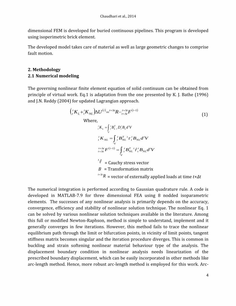
The governing nonlinear finite element equation of solid continuum can be obtained from

principle of virtual work. Eq.1 is adaptation from the one presented by K. J. Bathe (1996)

and J.N. Reddy (2004) for updated Lagrangian approach.

1

itt

tt

tti

NL

t

tL

t

t FRUKK (1)

Where,

VdBDBK t

L

t

t

V

t

T

L

t

tL

t

tt

VdBBK t

NL

t

t

V

tT

NL

t

tNL

t

tt

VdBBF t

NL

t

t

V

tT

NL

t

t

itt

ttt

1

t = Cauchy stress vector

B = Transformation matrix

Rtt = vector of externally applied loads at time t+Δt

The numerical integration is performed according to Gaussian quadrature rule. A code is

developed in MATLAB-7.9 for three dimensional FEA using 8 nodded isoparametric

elements. The successes of any nonlinear analysis is primarily depends on the accuracy,

convergence, efficiency and stability of nonlinear solution technique. The nonlinear Eq. 1

can be solved by various nonlinear solution techniques available in the literature. Among

this full or modified Newton-Raphson, method is simple to understand, implement and it

generally converges in few iterations. However, this method fails to trace the nonlinear

equilibrium path through the limit or bifurcation points, in vicinity of limit points, tangent

stiffness matrix becomes singular and the iteration procedure diverges. This is common in

buckling and strain softening nonlinear material behaviour type of the analysis. The

displacement boundary condition in nonlinear analysis needs linearization of the

prescribed boundary displacement, which can be easily incorporated in other methods like

arc-length method. Hence, more robust arc-length method is employed for this work. Arc-


5

length method originally developed by Riks (1972; 1979) and Wempner (1971) and later

modified by several researchers.

2.2 Arc length method Though this method is developed in 70s there are number of modification has been

suggested in past few years. One can find elementary of the method from any standard

literature either from Riks (1972, 1976) paper or Crisfield, 1981 etc. Generally there are

two approaches are used, a fixed arc length and varying arc length. The fixed arc length is

suitable for load and/or forced controlled, while for path following method, new arc-length

is evaluated at the beginning of each load step to ensure the achievement of the solution

procedure. The success of the path following method depends on three essential stages.

Firstly, proper selection of root for quadratic equation obtained by simplifications of the

additional constrains equation, which leads to a quadratic equation in terms of the

incremental load factor. Secondly, predicting value of the load-factor for at each increment.

Generally, load-factor for current increment is computed depending on the rate of

convergence of the solution process in previous increment. For first increment, trial value

is assumed as 1/5 or 1/10 of total load (Memon et al 2004). Finally, to avoid the doubling

back of the equilibrium path, determination of the sign for the predicted load factor needs

sufficient alertness. In case of divergence from the solution path, the arc-length is reduced

and computations are done again.

Figure 1. Iterative procedure for arc length method


6

Generally, incremental equations in structural nonlinear static analysis take the

following form

RFf ittittitt )1(11 (2)

Where, ftt

= the out of balance forceλ = a scalar, known as load levelparameter, which is

consider as an unknown parameter andR is a given fixed external force vector. The

incremental displacement for current load step with modified Newton-Raphson method

assumption of fixed KTis calculate as,

uuu ttittittitt ˆ111 (3)

Where 111 itt

T

itt fKu (4)

and

RKu T

tt 1ˆ (5)

Note that the KT is evaluated at the end of using the converged solution (t)u of the last load

step (Fig. 1). Hence improved prediction of the equilibrium configuration can be obtain as ittttt uuu

(6) 11 ittittitt uuu (7)

11 ittittitt (8)

For the first iteration of the first load step it is assumed that u = 0, for the first iteration of

other than first load step 11 t

can be calculated from incremental arc-length form written

as,

222 lRRuu (9)

Where Δu and λ are converged incremental quantities, ∆l is fixed radius of desired

intersection, and ψ is the scaling parameter for loading terms, for cylindrical arc-length

method, ψ = 0 (Crisfield, 1981); while for the spherical arc-length methods ψ = 1. For

cylindrical arc-length Eq. 9 simplified as,

2luu ittitt

(10)

Substituting for itt u from Eq. 7 gives quadratic equation for incremental in the load

parameter 1 itt u ,

03

1

2

21

1 AuAuA ittitt (11)


7

Where

uuA tttt ˆˆ1

uuuA ttittitt ˆ2 11

2

21111

3 luuuuA ittittittitt

To avoid the tracking backing the equilibrium path Crisfield suggested the root should be

such that, the angle between the incremental solutions at two consecutive iterations 1 iu

and iu be minimum. The incremental load factor λ is updated according to Eq. 8.

2.2.1 The Predictor solution

The auto-selection and auto-adjustment of the arc-length increment in each incremental

step are very important, which are related to the correctness and efficiency of the

numerical algorithms. In order to do that, the convergent information in the last arc-length

incremental step is very useful and must be analyzed. The main equations in controlling the

arc-length increments available is as follows n

dttt

I

Ill

0 (12)

Where tΔl is the arc-length used in the last iteration of last increment, Id is the number of

desired iterations (usually < 5) and I0 is the number of iterations required for convergence

in the previous step. Crisfield suggested that n should be set to ½. The first arc-length is

computed as

uul ˆˆ 1111 (13)

Hence, the incremental load factor for cylindrical arc length method can be

predicted as

uu

l

ˆˆ)(

11

11

(14)

The choice of the sign of the incremental load factor in the predictor phase of arc-length

methods is known to be of paramount importance in determining the success of such

procedures in tracing unstable equilibrium paths. If the wrong sign is predicted, the

solution sequence `doubles back' on the original load-defection curve and the arc-length

method fails to trace the complete path.Many procedures have been proposed to predict

the continuation direction, i.e., to choose the sign of δλ in the predictor solution such that it


8

does not `track back' on the current path. The most popular ones appear to be the

predictors based on

(a) The sign of current tangent stiffness determinant. Follow the sign of |KT|

sign(δλ) = sign(|KT|)

(b) Incremental work. Follow the sign of the predictor work increment:

sign(δλ) = sign (Tu R)

(c) The predictor criterion of Feng Follow the sign of history of the current

equilibrium path and the current tangential solution.

sign(δλ) = sign (Tu Δu)

Procedure (a) is widely used and works well in the absence of bi-furcations. In the presence

of bifurcations, however, it is known not to be appropriate and fails in most cases. As

pointed out by Crisfield, its ill behaviour stem from the fact that the sign of | KT| changes

either when a limit point or when a bifurcation point is passed. In this case, the predictor

cannot distinguish between these two quite different situations, unless further analyses are

undertaken. In the presence of a bifurcation, instead of following the current path, the

solution will oscillate about the bifurcation point. E.A. de Souza (1999) stated that the

procedure (b), on the other hand, is `blind' to bifurcations and can continue to trace an

equilibrium path after passing a bi-furcation point. However, this criterion proves

ineffective in the descending branch of the load-defection curve in `snap-back' problems,

where the predicted positive `slope' will provoke a `back tracking' load increase. Feng et al

(1996) proposed a direction prediction criterion (c). Whereby the sign of the predictor load

factor is made to coincide with the sign of the internal product between the previous

converged incremental displacement Δu and the current tangential solution, Tu .A key

point concerning the above criterion is the fact that Δu carries with it information about the

history of the current equilibrium path. E.A. de Souza (1999) shown by means of geometric

arguments that the resulting predictor of Feng et al (1996) approach can easily overcome

the problems associated with criteria (a) and (b).

2.3 Validation of code

For the validation of developed code, tests have been performed on the 3Dcantilever beam. Load- deflection curve is compared with commerciallyavailable finite element package ANSYS-12. Material behavior assumedfor the test is same as pipe material. Beam dimensions, meshing and pointload considered at free end are given in Table 1. Figure 2 shows perfectly matching load-deflection curve obtained from developed code and ANSYS.


9

Figure 2. Comparison of results between ANSYS and FE code.

Table 1. Comparison of Code and ANSYS results

L x D x B

(m)

Element size

(m)

Point load

(kN)

Umax(m)

Model ANSYS

3.0 x 0.2 x 0.05 0.05 x 0.05 x 0.05 80 0.130 0.135

2.4 Model dimensions

The coordinate system and notations used for this work are shown in Figure3. In reality,

soil media does not have any fixed boundaries or can beassumed at infinite distance,which

is virtually impossible to incorporatein numerical model, hence model dimensions are

determined for boundaryeffect and it considered as 80m (L) x 12m (H) x 15m (W).

(a) (b)

Figure 3 (a). Plan view of buried pipeline model for strike-slip fault motion. (b)Sectional view of

buried pipeline model for dip-slip fault motion.


10

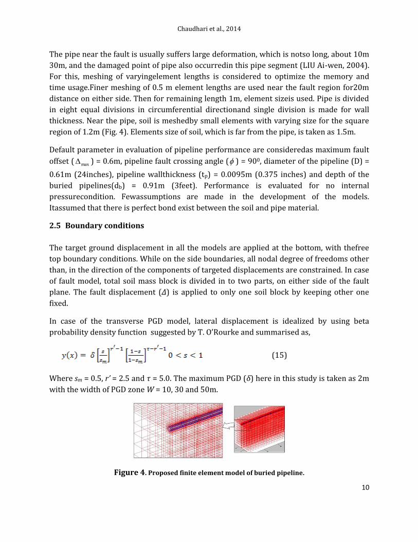
The pipe near the fault is usually suffers large deformation, which is notso long, about 10m

30m, and the damaged point of pipe also occurredin this pipe segment (LIU Ai-wen, 2004).

For this, meshing of varyingelement lengths is considered to optimize the memory and

time usage.Finer meshing of 0.5 m element lengths are used near the fault region for20m

distance on either side. Then for remaining length 1m, element sizeis used. Pipe is divided

in eight equal divisions in circumferential directionand single division is made for wall

thickness. Near the pipe, soil is meshedby small elements with varying size for the square

region of 1.2m (Fig. 4). Elements size of soil, which is far from the pipe, is taken as 1.5m.

Default parameter in evaluation of pipeline performance are consideredas maximum fault

offset ( max ) = 0.6m, pipeline fault crossing angle ( ) = 900, diameter of the pipeline (D) =

0.61m (24inches), pipeline wallthickness (tp) = 0.0095m (0.375 inches) and depth of the

buried pipelines(db) = 0.91m (3feet). Performance is evaluated for no internal

pressurecondition. Fewassumptions are made in the development of the models.

Itassumed that there is perfect bond exist between the soil and pipe material.

2.5 Boundary conditions

The target ground displacement in all the models are applied at the bottom, with thefree

top boundary conditions. While on the side boundaries, all nodal degree of freedoms other

than, in the direction of the components of targeted displacements are constrained. In case

of fault model, total soil mass block is divided in to two parts, on either side of the fault

plane. The fault displacement (Δ) is applied to only one soil block by keeping other one

fixed.

In case of the transverse PGD model, lateral displacement is idealized by using beta

probability density function suggested by T. O’Rourke and summarised as,

(15)

Where sm = 0.5, r’ = 2.5 and τ = 5.0. The maximum PGD (δ) here in this study is taken as 2m

with the width of PGD zone W = 10, 30 and 50m.

Figure 4. Proposed finite element model of buried pipeline.


11

2.6 Material modeling

The For pipe Ramberg-Osgood relationship is one of the most widely usedmodels (M.

ORourke(1999), IITK-GSDMA GUIDELINES (2007)), whilefor soil hyperbolic is common

(S.L Kramer (2007)). Hence, the same areused in these studies which aresummarized

below.

(16)

Where,

ε = Engineering strain

σ = Stress in the pipe

Ei = Initial Young’s modulus

σy = Yield strain of the pipe material

r, n = Ramberg - Osgood parameters adopted as r = 31.50 and

n= 38.32 Karamitros (2007)

While the hyperbolic soil model is given as,

(17)

where

τ = shear stress,

γ = shear strain

Gmax = maximum shear modulus

τmax = maximum shear stress

The API5L-X 65 steel pipe is frequently used in literature (NewmarkHall (1975),

Karamitros (2007) etc) hence the same is adopted for this study.Table 2 show the

properties used for API5L-X 65 pipe material. While soilis assumed as typical sand with

initial Youngs modulus as Ei = 50Mpa andPoisson ratio 0.4. Table 3 show constants used in

hyperbolic model.

Table 2: Properties of AP15L-X 65 Pipe

Properties for API5L X-65 Pipe Magnitude

Initial Young’s Modulus (Ei) 210 Gpa

Yield Stress (σy) 490 Mpa

Failure Stress (σf) 513 Mpa

Failure Strain (εf) 4%

Poisson’s ratio (μ) 0.3

Density (ρp) 7.8g/cm³


12

Table 3. Constants for Hyperbolic Model

3. Results and Discussion

The performance of continues buried pipeline crossing active fault is studied using

proposed finite element models. The developed model can implemented for all sort of fault

motion with variation in other geometric parameters. Here case of strike slip is taken to

determine the influencing on the performance of pipeline for the fault offset ( ), pipeline-

fault crossing angle ( ), wall thickness to diameter ratio (D

t p ) depth of the buried pipeline

(db) and their combinations. In the nonlinear numerical analysis of soil maximum ground

displacements is generally restricted up to 5% of the total depth of the model beyond

which results usually deviate and are unrealistic, hence maximum component of fault offset

is limited to 0.6m. Total fault offset of 0.6m is applied with an increment of 0.1m. Pipeline

fault plane angle is varied from 400 to 1400 with an increment of 100. The pipeline wall-

thickness 0.0095, 0.0103 and 0.0190 are considered, while depth is varied 2 to 4 feet.

3.1 Pipeline subjected to Strike Slip fault motion

3.1.1 Effect of the Fault offset

Hence for = 900 pipeline mainly subjected to the bending; while for positive small

angle pipeline will be under pure compression. Hence, for determining the effect of the

fault offset 600 angles is chosen, where effect of both the direct and bending strain can be

seen. Figure 5 shows the effect of the fault offset on total and bending strain distribution in

the pipeline. Maximum fault offset 0.6m is applied with an increment of 0.1m. Generally

two kind of failure are associated with pipeline, first material failure when pipe material

strained beyond sustain limit in general yield strain and geometric failure in which

geometry of the pipe is so distorted that pipeline becomes inadequate to pass the fluid.

From figure 5 (a) it can be seen that maximum strain ( xx = 0.00186) generating in the

pipeline for fault offset 0.2m is just below the yield strain ( y = 0.002). From whichit can be

said that pipe do not have any serious damage up to 0.2m faultoffset. Thereafter the

difference of the strain curve, near the fault planecontinuously increases. This indicates

Medium density sand properties Magnitude

Maximum Shear Modulus (Gmax) 60 Mpa

Maximum shear Strength (τmax) 0.0216 Map

Failure Stress (σf) 513 Mpa

Density (ρs) 1.44/cm³


13

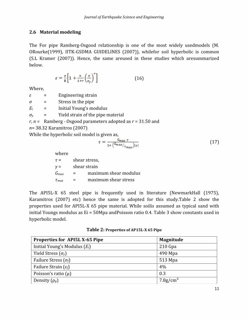
that pipe material entered in plasticstage. While discussing about the pipeline damage

there are two points, which are most significant. First, how much material has yielded

andsecondly how much length of the pipe enters in the plastic stage. This has great

significance in case of post event repair and maintains. This large longitudinal strain in the

pipe material further causes reduction in the wall thickness (developing upon Poisson

ratio), which may not be safe design thickness for the internal pressure and other load.

From the figure 5(a) one can see that for the 0.3m fault offset only near the fault plane

about10m pipe length is beyond the yield strain. While majority of the pipe length is just

crosses the yield strain. There after both length of pipeline crossing yield point and

maximum strain beyond the yield strain increasing seriously. For the considered cases no

large geometric failure is observed. From bending strain distribution curves (Fig. 5b) one

can observe that bending strain in the pipe is smoothly increasing up to the 0.4 fault offset.

After that bending strain distribution curve slightly disturbing for 0.5 and0.6m fault offset

at 10m on either side of the fault plane. This kind of disorder mainly signifies the local

buckling on the pipe.

Figure 5. Effect of fault offset on strain distribution for strike slip with Δy = 0.1m to 0.6 m

andϕ=600(a) Total strain effect. (b) Bending strain effect.

3.1.2 Effect of the Pipeline Fault Angle

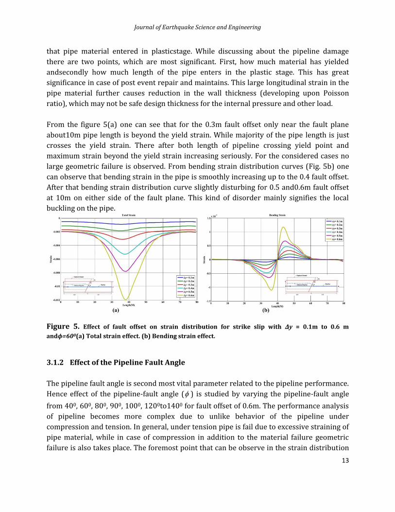
The pipeline fault angle is second most vital parameter related to the pipeline performance.

Hence effect of the pipeline-fault angle ( ) is studied by varying the pipeline-fault angle

from 400, 600, 800, 900, 1000, 1200to1400 for fault offset of 0.6m. The performance analysis

of pipeline becomes more complex due to unlike behavior of the pipeline under

compression and tension. In general, under tension pipe is fail due to excessive straining of

pipe material, while in case of compression in addition to the material failure geometric

failure is also takes place. The foremost point that can be observe in the strain distribution


14

curve plotted in figure 6 is maximum strain developing for negative pipeline fault angle

( < 900) is much higher than the positive pipeline fault crossing angle ( >900). The reason

for this can be understood as, when pipeline is subjected to the compression pipe has a

chance of bending and/or buckling and hence the fault offset is accommodate by the

geometric change without much internal deformation, which leads to lesser internal

deformation in the pipe. There are two fundament troubles associated with the pipeline

buckling, firstly it is a sudden phenomenon and may have an adversely affect the

operational pipelines.

Secondly, the large geometric distortion during buckling further causes pressure loss in the

pipeline, which is the foremost significant parameter for the petroleum pipeline. In case of

pipeline is under tension whole fault displacement at the pipe fault crossing is needed to

accommodate by the internal deformation of pipeline material.

Figure 6. Effect of pipeline fault angle on total normal strain distribution for strike slip with Δy

=0.6m

From figure-6 it can also observe that for ±800angle total normal strain distribution are

similar on the opposite side of zero strain axes. This indicates that thebuckling of the pipe

does not take place for all pipeline fault angle.

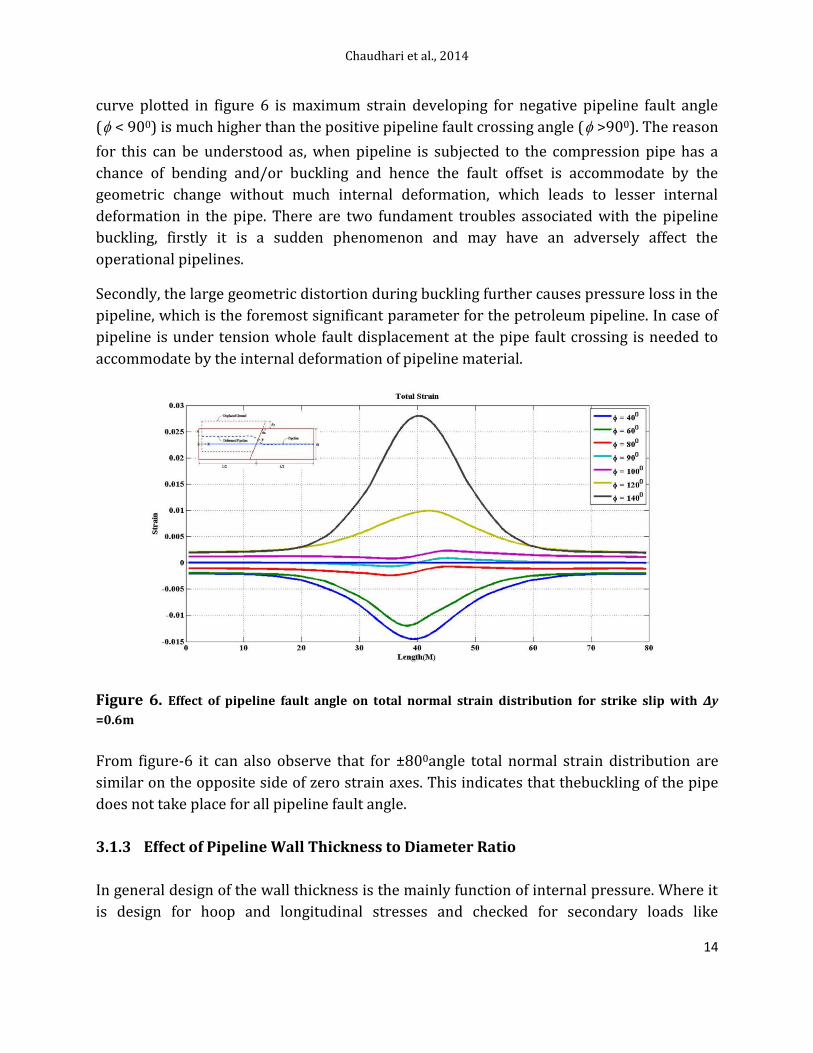
3.1.3 Effect of Pipeline Wall Thickness to Diameter Ratio

In general design of the wall thickness is the mainly function of internal pressure. Where it

is design for hoop and longitudinal stresses and checked for secondary loads like


15

overburden and live loads. Nevertheless, the present study shows that thickness to

diameter ratio has great hold on the pipeline performance crossing strike slip fault

especially when pipeline subjected to the compression. To understand the effect of the wall

thickness here 0.0095, 0.0136 and 0.0190 are the three wall-thicknesses to diameter ratios

considered. To have an effect of geometric failure under compression parametric study is

performed for = 400 where pipe can be subjected to sufficient compression.The

maximum fault offset here could able applied is 0.47m after which pipe subjected to large

geometric changes which further causes soil failure and diverges numerical analysis.

Figure 7. Effect of pipeline wall thickness to diameter ration for strike slip with Δy = 0.46m and ϕ =

400

Geometric failure of the pipe can be more clearly understood byobserving the deform pipe

hence for deformed shapes of the pipes with different wall thickness to diameter ratios are

plotted in figure 7. From figure, it can be clearly seen that pipe with thicker wall thickness

subject to more geometric changes than the pipe with thinner wall thickness.However,

thicker wall pipe has higher internal deformation capacity, whichcan be observer in the

strain distribution figure 8. Nevertheless, for less strain thicker pipe got more damage this

clearly indicates geometric failureof the thick wall pipe. The reason for this is quite

understandable that thinner wall pipe has lesser moment of inertia can be easily bent and

deform to accommodate the fault displacement. On other hand thicker wall pipe, which

subjected to less strain indicate that lesser internal deformation, therefore thick wall pipe

needs to accommodate fault displacement by large geometric deformations. From the

above discursion, it is clear that when pipe is subjected strike-slip fault with < 900,

thicker pipe are more vulnerable to geometric failure.


16

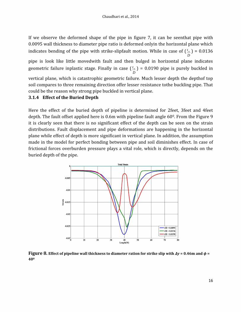
If we observe the deformed shape of the pipe in figure 7, it can be seenthat pipe with

0.0095 wall thickness to diameter pipe ratio is deformed onlyin the horizontal plane which

indicates bending of the pipe with strike-slipfault motion. While in case of (D

tw ) = 0.0136

pipe is look like little movedwith fault and then bulged in horizontal plane indicates

geometric failure inplastic stage. Finally in case (D

tw ) = 0.0190 pipe is purely buckled in

vertical plane, which is catastrophic geometric failure. Much lesser depth the depthof top

soil compares to three remaining direction offer lesser resistance tothe buckling pipe. That

could be the reason why strong pipe buckled in vertical plane.

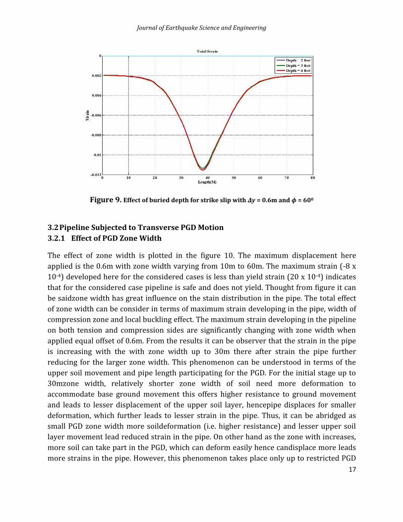
3.1.4 Effect of the Buried Depth

Here the effect of the buried depth of pipeline is determined for 2feet, 3feet and 4feet

depth. The fault offset applied here is 0.6m with pipeline fault angle 600. From the Figure 9

it is clearly seen that there is no significant effect of the depth can be seen on the strain

distributions. Fault displacement and pipe deformations are happening in the horizontal

plane while effect of depth is more significant in vertical plane. In addition, the assumption

made in the model for perfect bonding between pipe and soil diminishes effect. In case of

frictional forces overburden pressure plays a vital role, which is directly, depends on the

buried depth of the pipe.

Figure 8. Effect of pipeline wall thickness to diameter ration for strike slip with Δy = 0.46m and ϕ =

400


17

Figure 9. Effect of buried depth for strike slip with Δy = 0.6m and ϕ = 600

3.2 Pipeline Subjected to Transverse PGD Motion

3.2.1 Effect of PGD Zone Width

The effect of zone width is plotted in the figure 10. The maximum displacement here

applied is the 0.6m with zone width varying from 10m to 60m. The maximum strain (-8 x

10-4) developed here for the considered cases is less than yield strain (20 x 10-4) indicates

that for the considered case pipeline is safe and does not yield. Thought from figure it can

be saidzone width has great influence on the stain distribution in the pipe. The total effect

of zone width can be consider in terms of maximum strain developing in the pipe, width of

compression zone and local buckling effect. The maximum strain developing in the pipeline

on both tension and compression sides are significantly changing with zone width when

applied equal offset of 0.6m. From the results it can be observer that the strain in the pipe

is increasing with the with zone width up to 30m there after strain the pipe further

reducing for the larger zone width. This phenomenon can be understood in terms of the

upper soil movement and pipe length participating for the PGD. For the initial stage up to

30mzone width, relatively shorter zone width of soil need more deformation to

accommodate base ground movement this offers higher resistance to ground movement

and leads to lesser displacement of the upper soil layer, hencepipe displaces for smaller

deformation, which further leads to lesser strain in the pipe. Thus, it can be abridged as

small PGD zone width more soildeformation (i.e. higher resistance) and lesser upper soil

layer movement lead reduced strain in the pipe. On other hand as the zone with increases,

more soil can take part in the PGD, which can deform easily hence candisplace more leads

more strains in the pipe. However, this phenomenon takes place only up to restricted PGD


18

zone width (e.g. in this case up to30m), thereafter the maximum upper soil displacement is

stabilized forgiven base ground movement.

Figure 10. Effect of zone width on strain for transverse PGD with = 0.6m and W = 10 m to 60m

However with the increment in the PGD zone with more pipe length isthen happens to

available for the accommodating the ground displacement.Hence, that distributes the strain

over large length that further shifts thepoint of contra-flexure apart, which increases the

compression zone widthof the pipe.

Another significant point here can be seen is the local buckling effect.For sure, the local

buckling of the pipe is a vast subject and cannot be coverin this work. However, few

observations here can be made from figure10. For the case of 20 and 30m zone width,

maximum strain level in thepipe is more or less same, though one can see that pipe

subjected to 30m zone width expose to higher buckling. The reason could be the pipeline

length under compression is increasing with the PGD zone width that makes lenderness

ration in compression, which can easily buckle. Strain drop forthe buckling cases are more

for example for the case of 10m and 50m zonewidth, maximum compressive strain levels

are same but pipeline subjectedto 50m zone width has higher positive strains.

4. Conclusions

Main conclusions of this study can be stated as following:

Numerical modeling of physical problem if implemented with latest updated

methods could yield much better results.

Apart from material behavior and its failure, geometrical behavior becomes

important when studies are done on pipes subjected to large ground motions.


19

Compression failure behavior of the pipelines is catastrophic innature as it leads to

sudden buckling. Which crucially depends on the pipe wall thickness.

A strike-slip numerical study of buried pipelines with different parameters has

shown the effect of both direct and bending strain.

Though here developed model is implemented on the strike slip fault motion but the

same can be implemented for other kind of ground motions.

References

Bathe, K. J (2002). Finite Element Procedures, Prentice-Hall of India Private Limited, New

Delhi.

Dimitrios K. K., D. B. George, and P. K. George (2007). Stress analysis of buried steel

pipelines at strike-slip fault crossings, Soil Dynamics and Earthquake Engineering,

27(3), 200–211.

Neto, E.A. de Souza, and Y.T. Feng (1999). On the determination of the path direction for

arc-length methods in the presence of bifurcations and snap-backs , Computer Methods

in Applied Mechanics and Engineering, 179, 81–89.

EERI, The Izmit (Kocaeli) (1999). Turkey, Earthquake of August 17, 1999, EERI Special

Earthquake Report.

Feng, Y. T., D. Peric, and D. R. J. Owen (1996). A new criterion for determination of initial

loading parameter in arc-length methods, Computers and Structures, 58 (3), 479–485.

IITK-GSDMA (2007). Guidelines for seismic design of buried pipelines.

Reddy, J. N. (2004). Introduction to nonlinear finite element analysis, Oxford University

Press.

Kennedy, R. P., R. A. Williamson, and A. M. Chow (1997). Fault Movement Effects on Buried

Oil Pipeline, Transportation Engineering Journal, 103(5), 617–633.

Liu, A. W.., Y. X. Hu, F. X. Zhao, X. J. Li, S. Takada, and L. Zhao (2004). An equivalent-

boundary method for the shellanalysis of buried pipelines under fault movement, Acta

Seismologica Sinica, 17(1), 150–156.

Memon, B. A., and X. Z. Su(2004). Arc-length technique for nonlinear finite element analysis,

Journal of Zhejiang University Science, 5(5), 618–628.


20

Newmark N. M., and W. J. Hall (1975). Pipeline design to resist large fault displacements,

U.S. National Conference on Earthquake Engineering, 416–425.

Riks, E. (1972). The application of Newton’s method to the problem of elastic stability,

Journal of Applied Mechanics, 39(4), 1060–1065.

Riks, E., (1979). An incremental approach to the solution of snapping and buckling

problems, International Journal of Solids and Structures, 15(7), 529–551.

Rourke, M. J., and X. Liu (1999). Response of buried pipelines subject to Earthquake Effects,

Multidisciplinary centre for Earthquake Engineering and Research, Monograph No.3.

Rourke M. J. (1988). Critical aspects of soil-pipe interaction forlarge ground deformation,

Proc., 1st Japan-US Workshop onLiquefaction, Large Ground Deformation and their

effects on Lifeline Facilities, 118-126

Takada, S, J. Liang, and T. Li (1998). Shell-Mode Response of Buried Pipelines to Large Fault

Movements, Journal of Structural Engineering, 44A, 1637–1646.

Wang, L. R. L., and Y. H. Yeh (1985). A Refined Seismic analysis and Design of Buried

Pipeline for Fault Movement, Earthquake Engineering and Structural Dynamics, 13(1),

75–96.

Wempner, G.A, (1971). Discrete approximation related to nonlinear theories of solids,

International Journal of Solids and Structures, 7(11), 1581–1599.

Ministry of Petroleum and Natural Gas Government of India, New Delhi (Economic

Division) (2011-12). Basic Statistics on Indian Petroleum & Natural Gas

finite element analysis of buried continuous pipeline ... · finite element analysis of buried...

Documents