FINITE ELEMENT ANALYSIS OF FOOTINGSAND MAT FOUNDATIONS

•III1111111111111111111111111IIIVI- .#88360#

ByMD. ABDUS SALAM MOLLA

A thesis

DEPARTMENT OF CIVIL ENGINEERINGBANGLADESH UNIVERSITY OF ENGINEERING

AND TECHNOLOGY, DHAKA

Submitted in partial fulfilment for the requirement of the Degreeof

MASTER OF SCIENCE IN CIVIL ENGINEERING

FINITE ELEMENT ANALYSIS OF FOOTINGSAND MAT FOUNDATIONS

Member

Member

Member(External)

Chairman(Supervisor)

o

February ,1995

Dr. A. M. M. SafiullahProfessor & HeadDepartment of Civil EngineeringBUET, Dhaka . .-

Approved as to the style and content by :

A thesis

ByMD. ABDUS SALAMMOLLA

Dr. Jalaluddin KhandokerChief Structural EngineerDesign Development Consultants Ltd.23, New Eskaton, Dhaka.

A.M.M, C".J1e."L----~ ~l _

tiMlJ-. U). L J) I--------------~----Dr. Abdul MuqtadirAssociate professorDepartment of Civil EngineeringBUET, Dhaka.

---------------------------------

.-OL-~ __KJ~~~Dr; Ahsanul KabirAssociate professorDepartment of Civil Engineering .BUET, Dhaka.

TO

MY

PARENTS

DECLARATION.

Declared that except where specific references are made to other investigatorsthe work embodied in this thesis is the result of investigation carried out bythe author under supervision of Dr. Ahsanul Kabir, Associate Professor ofCivil Engineering, BUET. Neither this thesis nor any part of it has beensubmitted or is being concurrently submitted for any other purpose (except forpublication).

~

Md. Abdus Salam MollaRoll No. 881216 F

..

IV

February, 1995.

ACKNOWLEDGMENT

The author wishes to express his sincere and profound gratitude toDr. Ahsanul Kabir, Associate Professor, Department of Civil Engineering,BUET, under whose supervision the work was carried out. Without hisaffectionate guidance and invaluable suggestions at every stage this workcould never have materialised.

Sincere gratitude is expressed to Mr. Quamrul Islam Siddique, ChiefEngineer, LGED who gave the scope to complete the work by providingposting to the author surrounding Dhaka.

Heartiest thanks are expressed to Farhana Rifat Alam for her patience andinspiration during the whole period work.

Appreciation is also due to Unique Computer Service, Green Road, Dhakafor neat composing and printing the thesis.

v

ABSTRACT

This thesis deals with the analysis of footings and mat foundation by finiteelement method. The foundation mats are modelled with thick plateelements which include 4 noded bilinear element, 8 noded serendipityquadratic element and heterosis element. All are based on Mindlin'sassumptions. Isoparametric, formulation is considered in the study. Innumerical computation Gauss integration rule together with reducedintegration technique is employed. The soil under the foundation isconsidered as Winkler medium and subgrade reaction (kg) concept is used.

----" -.-

The node springs are computed by using either the contributing areamethod or the shape function method at element level and added toappropriate diagonal terms of element stiffness matrix. Similady, thevertical as well as the rotational stiffness of piles ai'e added to elementstiffness matrix in case of pile foundation. Equation solving is performedusing the powerful' frontal solution technique. The convergence of solutionis checked by using both displacement and residual force norm criteria.

In Winkler foundation using a constant kg on a rectangular uniformlyloaded flexible base will produce constant settlements which is not inagreement with the Boussinesq solution., To make the displacementscomparable with Boussinesq solution, soil zoning suggested by Bowles isconsidered in the study and its effect on the numerical results are studied.The effects of mat rigidity on the behaviour of foundation are alsoconsidered.

Finite element program developed in the study is, mainly for foundationanalysis, but it is capable to analyse slab problems of any type. Theappropriate order of quadrature for 'different Mindlin plate elements havebeen examined. Moreover, a smoothing technique to calculate stressresultants of nodes from the stress resultants at Gauss points is developed.

Higher order elements used are found to be quite efficient in the analysis ofslab and foundation problems. For most of the cases convergence is foundwithin 2 to 3 iterations. For eccentric footing where soil footing separationoccurs about 10 iterations are required. Due to bilinear behaviour theperformance of 4 noded element under concentrated load is found to beunsatisfactory.

VI

1

1

2

3

44

1820202023262828

3030303233

INTRODUCTION

CONTENTS

LITERATURE REVIEW,

General

Scope of Present StudyLimitations

General

Spread Footing 4

Assumptions Used in the Design of Spread Footings 4Structural Design of Spread Footings 5Eccentric Footing 8

Pile Foundation 10Combined footing 11

Design of Combined Footing by Conventional Method 12ACI Method for Analysis of Combined Footings 12Classical Solution of Beam on Elastic Foundation 14Finite Difference Solution of Beam on ElasticFoundation 16

Finite Element Solution of Beam On .ElasticFoundation

Mat Foundation

Design of Mat FoundationConventional Method of Mat DesignApproximate Flexible MethodFinite Difference MethodFinite Grid Method

Finite Element Method for Mat Foundation

MINDLIN PLATE FORMULATION AND BASICPROCEDURES FOR FOUNDATION ANALYSISGeneral

Mindlin Plate FormulationEquilibrium Equation

Isoparametric Finite Element Representation

Vll

2.42.4.12.4.22.4.32.4.42.4.52.4.6

3.1

3.23.2.13.2.2

CHAPTER 11.1

1.21.3

2.3.5

CHAPTER 22.12.22.2.12.2.22.2.3

2.2.42.32.3.12.3.22.3.32.3.4

CHAPTER 3

3.2.3 The Element Stiffuess Matrix 353.3 Jacobean Matrix and Cartesian Shape

Function Derivatives 363.4 Shape Function 373.4.1 Hierarchical Formulation of Heterosis Element 403.4.2 Element Connectivity 413.5 Summary of Gauss Quadrature 413.5.1' Appropriate Order of Quadrature 433.6 Modelling, Mesh Layout and Grading 453.7 Soil Parameter 473.7.1 Modulus of Subgrade Reaction 473.7.2 Evaluation of Node Springs from Modulus of

Subgrade Reactioll (ks) 513.7.3 Soil Separation Consideration 533.7.4 Modulus of Subgrade Reaction and

Consolidation Settlements 543.7.5 Consideration for Pile Foundation 54

CHAPTER 4 COMPUTER IMPLEMENTATION 554.1 General 554.2 Overall Program Structure 554.3 Brief Description of Modular Routines 574.3.1 Subroutine FEMATF 574.3.2 Subroutine DIMMP 574.3.3 Subroutine INPUT 574.3.4 Subroutine NODEXY 594.3.5 Subroutine GAUSS 594.3.6 Subroutine SFR2 604.3.7 Subroutine JACOB2 604.3.8 Subroutine CHECKI 604.3.9 Subroutine CHECK2 614.3.10 Subroutine ECHO 614.3.11 Subroutine ZEROMP AND VZERO 614.3.12 Subroutine MINPB 614.3.i3 Subroutine LOADPB 614.3.14 Subroutine ALGOR 62"4.3.15 Subroutine INCRE:M 63

Vlll

'. , ... ' . ,..

4.3.16 Subroutine STIFMP 644.3.17 Subroutine MODPB 644.3.18 Subroutine BMATPB 654.3.19 Subroutine SUBMP 654.3.20 Subroutine FRONT 654.3.21 Subroutine RESMP 654.3.22 Subroutine GRADMP 664.3.23 Subroutine STRMP 664.3.24 Subroutine CONVMP 664.3.25 Subroutine OUTMP 674.3.26 Subroutine SMOTH 67

7479

69

69

92

9292

6868

Load 68

PERFORMANCE OF MINDLIN PLATEAND ITS CONVERGENCE

Conclusions

General

Square Slab Subjected to Uniformly DistributedSimply Supported Square Slab Subjected toConcentrated Load at CentreComparison of Numerical Factors a and B forUniformly Loaded Simply Supported Square Slaband Check for Convergence

Comparison of Numerical Factors a and B forCentrally Loaded Simply Supported Square Slaband Check for Convergence

GeneralSTRESS EVALUATION. SMOOTHING TECHNIQUE 80

80808591Conclusions

IX

APPROPRIATE ORDER OF QUADRATUREFOR MINDLIN PLATE ELEMENTSGeneral

Appropriate Order of Quadrature for Mindlin PlateElements in Slab Analysis

Smoothing Techniques

Checking the Performance of Smoothing Technique

5.4

5.6

5.15.25.3

5.5

7.17.2

CHAPTER 5

CHAPTER 6

6.16.26.36.4

CHAPTER 7

7.2.1 Reduced Integration Versus Full Integration 937.2.2 2x2 Gauss Integration 947.3 Appropriate Order of Quadrature of Mindlin Plate

Elements in Foundation Analysis. 997.3.1 Reduced Integration Versus Full Integration in Wall

Footing 997.3.2 Reduced Integration Versus Full Integration in

Square Footing 1037.3.3 2x2 Gauss Integration in Square Footing 1057.3.4 Reduced Integration Versus Full Integration in

Eccentric Footing 1067.4 Conclusions 107

CHAPTER 8

8.18.2

8.2.18.2.28.38.3.18.48.4.18.58.5.18.6

CHAPTER 9

9.19.29.3

THICK PLATE ANALYSIS OF FOOTINGSAND MAT FOUNDATION 108General 108Comparison of Maximum Moments ofWall Footingand Column Footing 108Wall Footing 110Square Footing 112Eccentric Footing 117Numerical Example of Eccentric Footing 117Pile Foundation 123Numerical Example of Pile Foundation 123Mat Foundation 129Numerical Example of Mat Foundation 129Comparing the performance of Shape Function andContributing Area Methods in Calculating Node

Springs and the Effect of Self Weight of Foundation 132

ANALYSIS OF FOOTINGS AND MATS WITHPARTICULAR REFERENCE TO SOIL ZONING 134General 134Relative Stiffness Parameters 135Modelling of Column Fixity for Combined footingand Mat. 136

x

9.49.4.19.4.2

9.4.3

CHAPTER 10

10.1

10.2

REFERENCES

Appendix A

Appendix B

Effect of Soil Zoning on Foundation BehaviourSpread FootingStrip Footing

Raft Foundation

CONCLUSIONS AND SUGGESTIONSConclusions

Recommenda tions

Sample Input Data and Line Printer Output forSlab and Foundation Problems.Some Additional Figures.

Xl

142142146

150

162162166

167

List of Primary Symbols Used

XlI

= modulus of subgt;ade reaction

=' vertical springs of soil (and piles)

= rotational springs of piles; i = X, Y

= multiplier for pile springs; i = 1,2,3

= least base dimension

= base length

= moment of inertia= eccentricity

= thickness of footing or slab

= effective depth of concrete

= modulus of elasticity of concrete= poisson's ratio of concrete

= stress-strain modulus of soil= poisson's ratio. of soil

= soil pressure

= vertical displacement

= rotations in xz plane and yz plane respectively= shear rotations in xz and yz planes

= vector of displacements= degt-ees of fi-eedom

= nodal d. o. f. of an element= vector of stress

= flexural contribution to 0

= shear contribution too

= elasticity matrix

= flexw-al contribution to D

= shear contribution to D

= plate rigidity= strain vector

= strain-displacement matnx

= shape function matrix

v, ~c

8 x, 8 y

<Px, <j>y

w

q

e

B

LI

t

dEc (or E)

d. o. f.

dioOf

u

Ni

D

Df. DB

DI::B

J

Kij

Kfij

Ksij

Mx,MyMxyQx, Qy1.J.'i (d)G

~ , 11

x,y, z

= Jacobian matrix

= element stiffness matrix

= flexural contribution to Kij

= shear contribution to Kij

= direct bending moments in x and y directions respectively.= twisting moment

= shear forces in xz and yz planes= residual force vector

= shear modulus

= non-dimensional curvilinear coordinates= Cartesian coordinates

= vector of body forces

= numerical factors for slabs (chap. 5)

= relative stiffness parameter for spread footings

= relative stiffness parameter for strip footings and matfoundations

xiii

Chapter 1

INTRODUCTION

1.1 General

The usual methods for analysis of foundations involve a hierarchy ofassumption. The first assumption that is generally made is that thefoundation mat is infinitely rigid. This allows determination of bearingpressure distribution (or pile loads in case of pile foundation) by simplestatics. This is typically inadequate assumption for large mat, since theflexibility of the mat relative to soil, results in significant pressureconcentration in the area of load application (also true for pile foundation fordistribution of applied load to individual piles) and appreciable relief in areasdistant from that area of load application. Once this approximate bearingpressure distribution is determined the analysis proceeds on the basis usualequivalent frame method which consider one way bending rather than a morecomplex two way analysis: This introduces the second major simplifyingassumption. For very rigid, symmetrical (geometry and loading) mats, restingon soft soil these assumptions do not introduce serious error. However, fortypical mats, significant economy is lost in some region of the mat while.inothers under design is areal possibility. This under design may be of twotypes-(i) inadequate section design and (ii) excess bearing pressure.

ACI committee 436 (1966)1 suggested an 'Approximate Flexible Method' forthe general case of a flexible mat supporting columns at random locationswith varying intensities ofload. This procedure is based on theories of circularplates on Winkler medium. Shukla2 recommends this method to calculatemoment, shear forces and deflections of mat foundation. This method,however, is computationally intensive. Tahsin3 used this method to calculatedeflections and moments of mat foundation. He describes this method asinadequate since it is based on functions derived for infinite plates and theresults near the edges of the plate are found unsatisfactory.

To address the limitations and errors of approximate methods, differentdiscrete element methods e.g., finite difference method, finite gird methodand finite element method are available. Due to availability.~f~lectroniccomputer discrete elemei;.t methods have become popular. But well knownfinite difference method has a number of limitations4 regarding boundarycondition, modelling of column fixity, modelling of column moments etc.

1

Moreover this method is tedious and difficult to model mat of arbitraryconfiguration. To eliminate the difficulties of finite difference method, finitegrid method was proposed by Bowless and described in his book first as finiteelement method. Infact, this method is based on stiffness method of structuralanalysis and uses beam.column element. But for better representation offoundation mat, finite element method with plate elements can be used. Forthis purpose two types of elements namely thin plate elements and thick plateelements can be used. In thick plate elements transverse shear deformation isconsidered while in the former this is ignored. But foundations are generallythick and it under goes some sort of transverse shear deformation. Hencethick plate elements are expected to model foundation behaviour morerealistically.

1.2 Scope of Present Study

For linear analysis, the finite element method is widely employed as a designtool. Developed countries are using such analysis for quite a some time. Dueto widespread use of computer, computer method as a design tool is nowbecoming popular even in Bangladesh. The aim of present study is to developa special purpose finite element program with Mindlin plate elements foranalysis of foundation. However, under the limited scope of present study thefollowing aspects have been investigated.

a) .The performance of different Mindlin plate elements in modellingfoundation.

b) The appropriate order of quadrature for Mindlin plate elements.

c) The behaviour of footings and mat foundations under different columnfixity models.

d) The moments of wall footing and column footing and their comparisonwith moments obtained using ACImethod.

e) The moments of mat foundation and their comparison with momentsobtained using different approximate methods.

f) Modelling the distribution of column moments to element nodesrepresenting column area.

g) The behaviour of footing under eccentric loading and soil separation.

h) The behaviour of pile cap regarding transfer of applied forces to individual'1 \~es. ~

2

i) The effect of soil zoning on the behaviour of footings and mats.

j) The effects of mat rigidity on the behaviour offoundations.

Further a smoothing technique is developed to calculate the stress resultantsof nodes from the stress resultants of Gauss points. For isoparametricelements, integration points are the best stress sampling points. The nodeswhich are the most useful output locations for stresses appear tb be the worstsampling points. Therefore this smoothing technique is used to calculate thestresses of nodes for all cases.

The program developed in the present study is primarily for the analysis offoundation, however it is capable to analyse slab of any type like one wayslab, two way slab, flat slab, flat plate etc.

1.3 Limitations

In the present study, the soil under the foundation is considered as Winklermedium, which utilises the concept of subgrade reaction (kg). In Winklerfoundation using a constant ks on a rectangular uniformly loaded flexible basewill produce constant settlements which is incompatible to the Boussinesqsolution4. From Boussinesq solution it is evident that the base contactpressure contributes settlements at other points i.e., the centre of a uniformlyloaded flexible base settles more than the edges. However to make thedisplacements comparable with Boussinesq solution soil zoning suggested byBowles are considered in the study.

Mindlin plate elements considered in the present study can not be applieddirectly to analyse stiffened plate. In stiffened plate, while both slab andbeams can be modelled with Mindlin plate elements, the beam elementsrequire transformation to the mid surface of the slab in order to match thenodal points. This is beyond the scope of present study. However anequivalent approximation can be made by calculating the plate rigidity D o~beam elements at the mid surface of the slab as {Et3/12(1-v2)} (1+12d2/h2),where d is the distance between the centres of particular beam and slab, histhe depth of particular beam. It is to be noted that in the present study thereis scope to change four material parameters namely elastic modulus (E),poisson's ratio (v), material thickness (t) and material mass density (p) foreach element. Therefore for analyses of stiffened plate, in addition tochanging thickness t, the elastic modJlus E should be modified for beamelements by multiplying it with (1+12d2/h2) during data input.

3

Chapter 2

LITERATURE REVIEW

2.1 General

The foundation is that part of a structure which transmits the load to theunderlying soil or rock. Foundation is interfacing of two materials with astrength ratio in the order of several hundred. As a consequence the loadmust be spread to the soil in a manner such that its limiting strength is notexceeded and resulting deformations are tolerable. Shallow foundationse.g., spread footing, combined footing and mat foundation accomplish thisby spreading the loads laterally while deep foundation (piles or caissons)distribute a considerable amount of the load vertically' rather thenhorizontally. However a combination of above two types of foundation may bealso used. In this chapter various methods and assumptions for the designof different types of foundation are briefly described.

2.2 Spread Footings

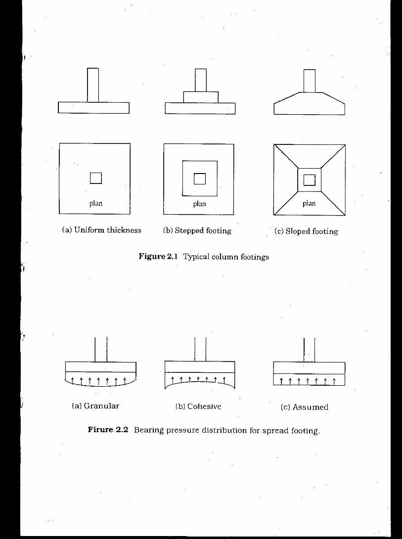
A footing carrying a single column is called spread footing and its functionis to spread the column load laterally to the soil so that the stress intensityis reduced to a value that the soil can safely carry. These members aresometimes called single isolated footings. Wall footings serve a similarpurpose of spreading the wall load to the soil.

In plan single column footings are usually square. Rectangular footing areused if space restrictions dictate this choice or if the supported columns areof strongly 'elongated rectangular cross section, In the simplest form singlefootings are of uniform thickness all over. However stepped or slopedfootings are also used. Common types of spread footing are shown inFig.2.1

2.2.1 Assumptions Used in the Design of Spread Footings

Analysis based on theory of elasticity indicates6 that pressure distributionbeneath symmetrically loaded footings is not uniform. The actualdistribution depends on both footing rigidity and base' soil. For footingsresting on coarse grain soil, the pressure is larger at the centre of the

4

footing and decreases towards the edges (Fig.2.2a). This is so because theindividual grains in such soils are somewhat mobile so that the soil locatedto the perimeter can shift very slightly outward in the direction of lower soilstresses. In contrast, in clay soils pressure are higher near the edge than atthe centre of the footing. The high edge pressure may be explained byconsidering that edge shear must occur before any settlement can takeplace. It is customary to disregard these non-uniformities7 (1) because theirnumerical amount is uncertain and highly variable due to interaction ofthe footing rigidity with the soil type, state and time response to stress, and(2) because t4eir influence on the magnitudes of bending moments andshear forces in footing is relatively small .Thus it is common practice to usea linear pressure distribution (Fig.2.2 c) beneath spread footings.

2.2.2 Structural Design of Spread Footings

Spread footing design is based almost entirely on the work of RichartS andMoe9. Richart's work contributed to locating the critical section formoments; critical shear sections are based on Moe's work. The ACI,AASHTO and AREA specifications4 for footing design are identical forlocation of critical section as suggested by Richart and Moe. In this context,the critical sections for bending moment in R.C. wall or column footings areconsidered the face of the wall or column. For footing supporting masonrywall, the maximum moment is computed midway between the middle andthe face of the wall. Spread footings have two critical sections against shearfailures, one for punching shear and other for wide beam shear. Thecritical section for punching shear is considered the vertical plane aroundthe column at a distance d/2 from ,the face of the column. The criticalsection for wide beam shear is considered the section across the footing at adistance d from the face of the column.

The allowable soil pressure controls the plan (BxL) dimensions of spreadfooting. Structural (or architectural) and environmental factors locate thevertical position of the footing in the soil. Shear stresses usually control thefooting thickness t. Two-way action shear (punching shear) always controlsthe depth of centrally loaded square footings. Wide beam shear may controlthe depth for rectangular footings when the .LIB ratio is greater than about1.2 and may control for other LIB ratios when there is overturning or

5

D

(e) Assumed

(c) Sloped footing

plan

(bl Cohesive

(b) Stepped footing

.

plan

Figure 2.1 Typical column footings

D

iii i

Firure 2.2 Bearing pressure distribution for spread footing.

(a) Granular

(a) Uniform thickness

eccentric loading.

Steps in square or rectangular spread footing design with a centrally loadedcolumn and no moments are:

1. The footing plan dimensions BxL are computed using the allowable soilpressure as :

P ~ltBxL=-, whereqa=--~ FS

A rectangular footing may have a number of satisfactory solutionsunless either B or L is fixed.

2. Since the footing plan dimension BxL computed as above is usuallyrounded to the nest higher 0.25 ft. or 0.50 ft, the soil pressure under thefooting is required to be adjusted as following:

Pa. q =PxL in WSD

Pub, q = BxL in USD where Pu is obtained by applying appropriate load

factors to the given design loading.

3. Considering the allowable two way action shear stress Ue the the effectivefooting depth d is computed.

4. Considering wide beam shear the effective footing depth d IS alsocalculated.The largest d from step 3 or 4 is used.

5. The bending moment is computed at the critical section shown inFig. 2.3. For the length I shown, the bending moment/unit width is

ql2M =- (2.1)

2

Using the bending moment of critical section the required steel area IS

computed.

As mentioned above the current ACI procedure of spread footing design formoment is based on tests by RichartB which show larger bending momentsat the column face for column strips and lesser values on other strips.Bowles4 using finite difference and finite element analytical procedure

7

2.2.3 Eccentric Footing

(2.2)

masonry wall

Critical ~ I~w/4section

1(b)Masonry wall footing.

8

R.CWall,coiumn or,pedestal exceptmasonry wall

ICritical ~

Section

1(a) R. C. wall, column or pedestal

footing

pq= A:t M.x/I

Figure2.3 Critical sections for computing bending moment.

In conventional analysis of rigid footings, the soil pressure can be computedfrom principles of mechanics of materials for combined bending and axialstresses. For moment about an axis perpendicular to the footing length L,the soil pressure can be computed when no footing separation occurs as

When footings have moments as well as axial loads, the soil pressureresultant will not coincide with the centroid of the footings as illustrated inFig. 2.4a and the footings are called eccentric footing. Footings with off-centre column (Fig. 2.4b) also produces similar effects and are classed aseccentric footings.

found that while the bending moment is higher in the column area,for finite difference methods the average bending moment across a squarefooting at the .critical section is the same as obtained using the codespecification. The maximum computed moment exce.eds the average byabout 30 percent for finite difference method and by more than 40 percentusing the finite element method. It is implicit that readjustment will takeplace to reduce the cracking effect of column-zone moment in the coderequirement. It may be questionable whether the 40 percent longer momentcan be adequately readjusted without possible cracking and long termcorrosion effects.

9

Figure2.4 Eccentric footings.

(2.3)

~PI CL,I

( I L ~,

-4e~R=P

(b) Footing with off-centrecolumn

-PMI,I

<:;-- L ' )

CL i~e~t, I R=l'

where B = width of the footing.A = area of the footing (BxL), other notations as shown in Fig. 2.4

(a) Footing with axial load andmoment.

When the soil resultant is exactly at the kern point the toe pressure is amaximum, while the heel pressure is zero and the average base pressure is~ax/2. When the resultant acts within the middle third no soil footingseparation would occur. However there are occasion when it is impossible tokeep soil resultant inside the middle one-third of the base. This situationoccurs when one or more of the design load combinations substantially

Pq = A :t Mx.x/ly:t My.y/lx (2.4)

_ .!... Bex+ Beyor, q maxor q min- BL (1:t L - B ) (2.5)

where Mx, Iy and My, Ix are moments and moment of inertia about Y axesand X axes respectively.ex = x-direction eccentricity.ey = y-direction eccentricity.

The soil pressure for footing with eccentricity about both axes can becomputed when no soil footing separation occurs as :

P Beor, qmaxorqmin = BL (1 :t""L)

(2.7)

exceeds the over turning capacity (transient or temporary load cases asfrom wind' or earthquake). While footings are not usually designed for thesecases they should be checked for overtuming stability under the temporaryloading. For situation some sort numerical solution to the problem will behelpful. Finite grid, finite difference and finite element method are some ofthe numerical methods that can be effective used for solution of biaxiallyloaded eccentric footings.

2.2.4 Pile Foundation

Piles are structural members of timber, concrete, and/or steel used totransmit surface loads to lower levels in the soil mass. This may be byvertical distribution ofthe load along the pile shaft or a direct application ofload to a lower stratum through the pile point or both.

Unless a single pile is used a cap is necessary to spread the vertical loadsand overtuming moments to all the piles in the group. The cap is usually ofreinforced concrete, poured on the ground unless the soil is expansive. Thepile cap has a reaction which is a series of concentrated loads (the pile) andthe design considers the column loads and moments, any soil overlying thecap and the weight of the cap. It is usual practice to assume that:

1. Each pile carries an equal amount of the load for a concentric axialload on the cap for n piles carrying a total load Q. the load Pp per pile is .Pp = Qln (2.6)

2. The combined stress equation (assuming a planar stress distribution)is valid for a pile cap which is not centrally loaded' or loaded with aload Qand a moment heaving components Mx and My. The pileloads may then be obtained as

Pp = Qln :t Myx :t MyYLX2Ly2

where Mx, My = moments in the x andy direction respectivelyx, y = distances from y and x axes to any pile

L x2, L y2 = moment of inertia of the group about Y and Xaxes, computed as1= 10 + Ad2

but 10 is negligible and the A term cancels, since it is the pile load

10

desired and appears in both the numerator and denominator of. Eq. 2.7.

The assumption that each pile in a group carries equal load may be nearlycorrect when the following criteria are all met:1. The pile cap is in contact with the ground.2. The piles are all vertical.3. Load is applied at the centre ofthe pile group.4. The pile group is symmetrical and the cap is very thick.

In a practical case of a four-pile symmetrical group centrally loaded, eachpile will carry one-fourth of the vertical load regardless of the cap rigidity.With a fifth pile directly under the load cap rigidity will be a significantfactor:

Pile cap moments and shears for design are best obtained by using a finiteelement or finite grid computer program.

2.3 Combined Footings

When a footing supports a line of two or more columns it is called acombined footing. A combined footing may have either rectangular ortrapezoidal shape or be series of pad connected by narrow rigid beams calleda strap footing.

When it is not possible to place columns at the centre of a spread footingbecause of property line restriction or adjacent column being so close to eachother that their footings would merge or mechanical equipment locations, itbecomes necessary to use combined footings to avoid the non uniform soilpressure. The footing geometry is made such that the centroid of the footingarea coincides with the resultant of the column loads. This footing and loadgeometry allows the designer to assume a uniform soil pressuredistribution.

A combined footing may be rectangular if the column which is eccentricwith respect to a spread footing carries a smaller load than the interiorcolumns. It will be trapezoidal-shaped if the column which has too limitedspace for a spread footing carries the larger load. In these case theresultant of the column loads (including moment) will be closer to thelarger column load and doubling the centroid distance as done for the

11

rectangular footing will not provide sufficient length to reach the interior. column. A strap footing may be used in lieu of a combined footing ofrectangular or trapezoidal shape if the distance between columns is largeand/or the allowable soil pressure is relatively high so that the additionalfooting area is not needed. Common types of combined footing are shown inFig. 2.5

2.3.1 Design of Combined Footings by Conventional Method

The basic assumption for the design of combined footing is that it is rigidmember so that the soil pressure is linear. The pressure will be uniform ifthe location of the force resultant (including column moment) coincideswith the centre of area.

The conventional (or rigid) design of combined footing (rectangular ortrapezoidal) consists in determining the location of the centre of the footingarea. The centre of the area is adjusted in such a way that it coincides withthe centre of resultant force. Thus the length and width can be found. Withthese dimensions the footing is treated as a beam supported by two or morecolumns and the shear and moment diagrams are drawn. The depth basedon the more critical of punching shear or wide beam shear are computed.Critical sections for two way action and wide beam are the same as forspread footings i.e., at d/2 and d respectively from the column face. It iscommon practice not to use shear reinforcement both for economy and toincrease the rigidity. With the depth selected, the flexural steel can be .designed using the critical moments from the moment diagram.

The additional considerations for strap footing is that strap must be rigidand should be out of contact from soil. Also that footing should. beproportioned for approximately by equal soil pressures and avoidance oflarge differences in B to reduce differential settlement.

2.3.2 ACI Method for Analysis of Combined Footings

A simplified procedurel has been developed which covers the most frequentsituations of strip and grid foundation. The method first defines theconditions under which a foundation can be regarded as rigid so thatuniform or overall linear distribution of subgrade reactions can be.assumed. This is the case when the average of two adjacent span length s in

12

Figure 2.5 Typical combined footings

I

-

Dplan

-

(bl Trapezoidal

(c). Strap

I

D D.

plan

-

plan D

(a) Rectangular

14

2.3.3 Classical Solution of Beam on Elastic Foundation

(2.8)

(2.9)

-\jkSBI-.= 4E 11._oJ

where ks.= Sks'ks '= coefficient of subgrade reaction in ksfS = shape factorB = width offooting, ft

Ec= modulus of elasticity of concrete, ksfI = moment of inertia offooting, ft4

where ks' = ksB. In solving the equation, a variable is introduced:

a continuous strip does not exceed 1.75/1-., provided that the adjacent spanand column loads do not differ by more than 20 percent of the larger value.Here,

If the average of two adjacent span exceeds 1.75/1-., the foundation isregarded as flexible. Provided that adjacent spans and colurim load differ byno more than 20 percent, the complex curvilinear distribution of subgradereaction can be replaced by a set of equivalent trapezoidal distribution. Withthis idealisation the design of continuous strip and grid footings mayproceed following procedures described in the previous sections .

When flexural rigidity of the footing is taken into account, a solution is usedthat is based on some form of a beam on elastic foundation. This may be ofthe classical Winkler solution10 in which the foundation is considered as abed of springs (Winkler foundation) or a finite element procedure of recenttimes.

The classical solution being of closed form, are not as general in applicationas the finite element method. The basic differential equation is

d4yEI-~-k '

dx4 s Y

. In recognition of the approximation and over design using conventional (orrigid) method, current practice tends to modify the design by a beam onelastic foundation analysis.

where

15

I{2cosh AXcos AX(sinh ALcosAacosh Ab--sin A1 cos(sinh2A1-sin2A1)

Aa cos Ab) + (cosh AXsin AX+ sinh Ax cos AX)[sinh AL(sin Aa cosh Ab-cos Aa sinh Ab) + sin AL (sinh Aa cos Ab- cosh I,a sin Ab)]}

1(sinh2AL _sin2AL) {2 sin AXsin AX(sinh AL cos Aa cosh Ab - sin AL

cosh Aa cos Ab) + (cosh AXsin AX- sinh AXcos AX)X [sinh AL (sin Aacosh I,b - cos Aa sinh Aa) + sin AL (sinh Aa cos Ab - cosh Aa sin Ab)]}

1(. . h2 L . 2'L) {(cosh Ax sin I,X + sinh AXcos AX)X (sinh AL cos I,asIn A - SIn "- . .cosh Ab - sin AL cosh Aa cos Ab) + sin AXsin I,X [sinh AL (sin Aa coshAb-cos Aa sinh Ab) + sin AL (sinh Aa cos Ab - cosh Aa sin Ab)]}

A' =

The classical solution presented above has several distinct disadvantagesover the finite element solution. some of these are:

1. It assumes weightless beam.

2. Difficult to remove soil effect when footing tends to separate from soil.

3. Difficult to account for boundary conditions of known rotation or

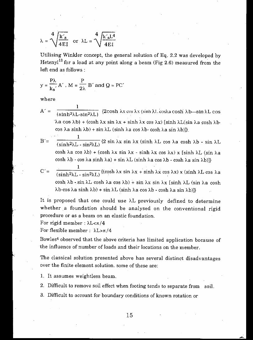
Utilising Winkler concept, the general solution of Eq. 2.2 was developed byHetenyill for a load at any point along a beam (Fig 2.6) measured from theleft end as follows:

_\!k'S _\!k'S14A - 4EI or A1 - 4EI

PA PY = -A' M = - B' andQ = PC'k' , 2As .

It is proposed that one could use I,L previously defined to determinewhether a foundation should be analysed on the conventional rigidprocedure or as a beam on an elastic foundation.For rigid member: A1<rc/4For flexible member: A1>rc/4

Bowles4 observed that the above criteria has limited application because ofthe influence of number of loads and their locations on the member.

deflection at selected points.

4. Difficult to apply multiple type of loads to a footing.

5. Difficult to change footing properties of!, D and B.

6. Difficult to allow for change in subgrade reaction along thefooting.

2.3.4 Finite Difference Solution of Beam on Elastic Foundation

The finite difference method treats the footing as a flexural memberconsisting of sections usually of equal length h. Instead of being supportedon a continuous soil pressure, each section is supported by equivalentconcentrated reactions RI, R2 etc, at panel points 1, 2 etc. (Fig. 2.7). Theforces and the reactions RI, R2 etc. should behave according to wellknown relationships for flexural members where

Deflection = y

dZYMoment, M = EI-

d(2.10)xZ

The above equations are substituted with the following finite differenceoperators:

Deflection at points 1, 2, 3 = Yl. Yz, Y3 .... etc.

dy ~y I Y3-Yzdx = ~x = h first forward difference

~YI Y2-YIor~x 2 = h first backward difference

Add' 2 liy I _ .Y3 -Ylmg, ~x 2 - h

d2y tl2y tl(tly/ tlx)The second dirivativ dx2 = tl2y/tlx2 can be expressed by tlx2 = tlx

which is equivalent to1 Y3 -Y2 Y2 -Ylh( h - h )

and simplifyingtJ.2y .. Y3-2Y2 + Yl.tJ.x2 = h2

16

-y

b

soil pressure

------B ------

I----L

~

'I

XP

,- f+y

1 h 2 h 3 h 4 h 5 h 6 h 7

t t t t t t tR[ R2 R3 RJ R, R6 R7

~IY3 I y, EVV7" .•.• " ) .•

detlection

Figure 2.6 Finite length beam on clastic foundation.

Figure 2.7 Equivalent finite difference approximation.

d2y (Yl - 2Y2 + Y3)Thus the moment at 2 =(dx2 ) EI = h2 EI

similarly the moment at other points are computed. Analysis ofcombined footing by means of finite difference method requires the followingsteps:

1. The footing is divided into 4 to 6 equal divisions, each oflength h.

2. Considering the deflections YI' Y2 etc. the soil reactions at points 1,2etc. are completed as Ylks, Y2ks,etc.

3. The continuous soil reactions are then replaced by equivalentconcentrated reactions RI, R2 etc.

4. The footing under the applied loads and equivalent reactions shouldsatisfy the equations of equilibrium i.e., IM = 0 and IV = O.The equation for the IM = 0 at any panelled points and IV = 0 for wholesystem in terms ofYl' Y2'etc. are written.

5. The resulting simultaneous equations are then solved for Yl' Y2' Y3etc.

It is seen that this method requires very little labour. The only tedious workis the solution of simultaneous equations. With the advance of digitalcomputers, this is no longer a tedious procedure. However, this methodmay not converge.

2.3.5 Finite Element Solution of Beam On Elastic Foundation

The finite element method is the most efficient means for solving a beam onelastic foundation type of problem. It is easy to account for boundaryconditions, beam weight and non linear soil effect including soil footingseparation.

For the analysis of combined footing by finite element method, beamelement can be used.

18

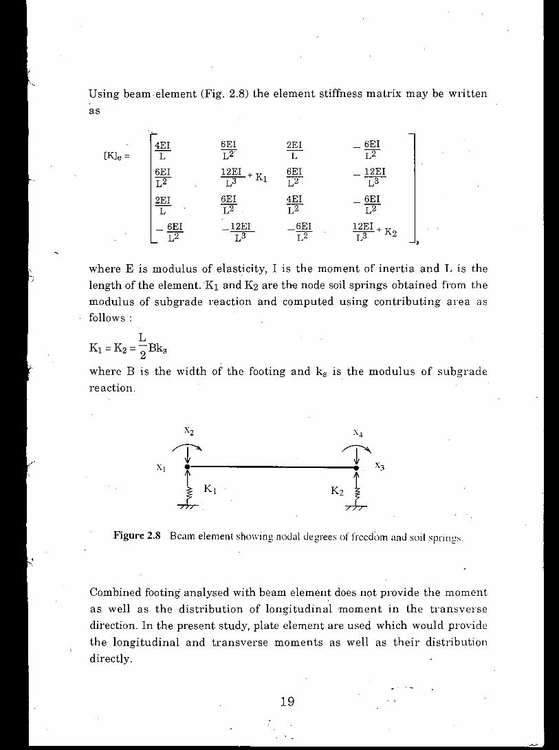
Using beam element (Fig. 2.8) the element stiffness matrix may be writtenas

4EI 6EI 2EI 6EI[KJe= L L2 L L2

6EI 12EI + K 6EI 12EIL2 L3 1 L2 IT2EI 6EI 4EI 6EIL L2 L2 L26EI 12EI 6EI 12EI + KL2 ~ L2 L3 2 ,

where E is modulus of elasticity, I is the moment of inertia and L is thelength of the element.Kl and K2 are the node soil springs obtained from themodulus of subgrade reaction and computed using contributing area asfollows:

LK1 =K2 = "2Bkswhere B is the width of the footing and ks IS the modulus of subgraclereaction.

X2 X.j

~ '1' X3Xl • •l' K21-l- KjFigure 2.8 Beam element showing nodal degrees or freedc)m and soil springs.

Combined footing' analysed with beam element does not provide the momentas well as the distribution of longitudinal moment in the transversedirection. In the present study. plate element are used which would providethe longitudinal and transverse moments as well as their distributiondirectly.

19

2.4 Mat Foundation

A mat foundation may be used where the base soil has a low bearingcapacity anclJor the column loads are so large that more than 50 percent ofthe area is covered by conventional spread footings. It is common to use matfoundations for basements to spread the column loads deep in to a bettersoil strata and to provide the floor slab for the basement. A particularadvantage for basements at or below the ground water table that it acts as awater barrier.

Mat foundation may be supported by piles in situations such as high groundwater level ( to control buoyancy) or where the base soil is susceptible tolarge settlements. It should be noted that the mat contact stress willpenetrate the ground to a grater depth which shall have relatively higherintensity at a shallower depth- both factors tend to increase settlementsunless there is a stress compensation from excavated soil so that the netincrease in pressure is controlled. Common types of mats are shown in Fig.2.9.

2.4.1 Design of Mat Foundation

There are several methods which can be used to design a mat foundation:

1. Conventional Method.

2. Approximate flexible method

3. Discrete element method.

a. Finite differenf:e methodb. Finite grid method (FGM)c. Finite element method (FEM)

2.4.2 Conventional Method of Mat Design

In the conventional method it is assumed that the mat is infinitely rigid andthat bearing pressure distribution against the bottom of the mat follows aplanar distribution. Since a mat occupies the entire area ofthe building it isoften unfeasible and uneconomic to proportion the mat so that the centriodof the mat coincides with, or is close to, the line of action of the resultantforce.

20

Figure2.9 Common types of mat foundations.

E ~---; ~---; i--~~---; Et ~__~ ~__J ~ __ J ~._J t

r--., ,..--, roo, ,.__~~-" ,. "_!r " " I I II.. __ J '-- __ oJ '- __ J '- __ J,...--.,r--, .---, r--,I " , I " II , I " II ,L __ J '- __ -' L __ J '- __ .J

~~ £.£

(e) basement wallsas part of mat

(d) plate withpedestals

WE-O.D

EI3£l aJ:fl aJ:flA-A B-B C-C

A • • • • • A B .' (~; (!'} 'f C •r-,. r-,.r-,. r-,.-' Ct t tI,~'I ~!r t I , I I I , , ,

t:~I~~) ~!; t_J '-.J 1...-' L.J

I • • • • • L • •••• -'r-, ....--, r-, r-,-- '_1", " ..........• • • • • :~.~~;'~~,jI:, \.~ L.J I...J '-.J '-.J• • • • •,-, ,-, ,-, ,-,, , , , , ,• • • • • Ii) ',ie \.~

'.~ :i,-, '-' c _, C_,• • • • •

(a) flat plate (b) plate thickened (c) waIDe -slabunder column

(2.11)

The procedure of design by conventional method consists of the followingsteps:

1. The line of action of all loads acting on the mat is determined.

2. The pressure distribution can be determined by the following formula

1 ex.x ey.yq= R(- + - + )

A Iy Ixwhere R = LQ = total vertical loads on the mat.

A = total area of the mat

x, y = coordinates ,ofany given point on the mat with respect to the

X and Y axes passing through the centriod of the area of the mat.

ex' ey = coordinate of the resultant force,

Ix, Iy = moment of inertia of the area of the mat with respect to the

X and Y axes respectively ..

3. The mats analysed as a whole in each of two perpendicular directions

and the shear and moment are determined from the principles of statics.

Thus, the total shear force acting on any section cutting across the entire

mat is equal to the arithmetic sum of all forces and reactions (bearing

pressure) to the left, or right of the section. The total bending moment

acting on such section is equal to the sum of all moments to the left, or

right, of this section.

Although the total shear and moment can be determined by the principle of

statics, the stress distribution along this section is a highly indeterminate

problem. In order to obtain some idea as to the upper limit of stresses, each

strip bounded by centre lines of column bays may be analysed as

independent, continuous, or combined footings. Full column loads are used

and the soil reaction under each strip is determined without reference to the

planar distribution determined with the mat as a whole. This method

undoubtedly gives very high stresses because it ignores the two way action of

the mat. Therefore, certain arbitrary reduction of stresses12 (for example-15percent, 25% percent, sometimes as great as 33 percent) are used.

According to the ACI committee436 (1966)1 a mat may be regarded as rigid

22

if the column spacing is less than llA (Eq. 2.1 defines A) and column

spacing do not vary more than 20 percent of the greater value and the design

is based on statics (conventional method). On the other hand if the column

spacing exceeds l/A. provided that the variation of adjacent column load

and spans is not greater than 20 percent. the same simplified procedure as

for strip and grid foundation described earlier can be applied to mat

foundations. The mat is divided into two sets of mutually perpendicular

strip footings of width equal to the distance between mid spans and the

distribution of bearing pressures and bending moments is computed for

each strip as explained before. Once moments are determined, the mat in

essence is treated like a flat slab or plate, with the reinforcement allocated

between column and middle strips.

2.4.3 Approximate Flexible Method

ACI committee 436 (1966)1 suggested this method for the general case of a

flexible mat supporting columns at random locations with varying

intensities of load. This procedure is based on theories of circular plate on

Winkler medium. Shukla2 recommends. this method to calculate momentshear forces and deflections .of mat foundation.

The approximate flexible method requires the following steps:

1. Over all thickness of mat is calculated from shear requirement

(usually two-way action shear) at critical section.

2. The plate rigidity is then calculatedE t3

D= C12(I~fle2)

where Ee = Modulus of elasticity of concrete.

t = Thickness of the mat

fIe = Possion's ratio of mat concrete.

3. The radius of effective stiffness L is computed as

23

24

An illustration of computations for a mat are given by Shukla2 by using this

procedure; however, the D calculated in this reference is in error so that the

resulting computations are not quite correct.

(2.17)

(2.18)

and My in teI'ms of rectangular coordinates5. The design moments Mx

can be computed as

Mx = ~cos2e + ~ sin2e

My = ~ sin2e + ~ cos2e

L=_4 fD-\j~

where ks = modulus of subgrade reaction.

The approximate zone of any column influence is 4L.

PV = - -Z' (2.14)4L 4

PL2~ = - (at load) (2.15)

3D

PL2~ = 4D Z3 (at a distance r from load) (2.16)

where x = distance ratio rlL

Mt• Mr = tangential and radial moments per unit width

V = shear per unit width of plate.

Zi = factors from Hetenyill and shown in Fig. 2.10

4. The radial and tangential moments. the shear and deflection are

computed using the following equations:

P 1-rtMr = - - [Z =-=Z' ] (2.12)

4 4 x 3

P 1-rtMt = - - [rt Z +.::...:.:.c. Z' ] (2.13)

4 c4 x 3

Figure2.10 Zi factors for computing deflections, moments andshears in a flexible plate.

654Jx = r/L

2o

\- Z'IY

\1\ M,~> .•.Ll'\- z~ ~'~tr:'M,hI'\ M;r = M,cos28+ M,sin28

~.'vi}' = At, sin2 e + M, cos2 8

I ,X=-

I \ L

if:I " '" L~ -k •£<r3

1 I /"" -.:::::t-- D

12(1 - ";)--I V -- -~?

I, il " I"1

1 !I /1\

\1 , LL Z,l- )/1

1I ,

1I

J12•

1 1I

I1I

5

0.:

0.5

0.3

0.1

0.4

-0.

-0.

-0.2

-0.

-0.4

The finite difference method uses the fourth order differential equation

(2.20)

(2.19)P

D(dxCJy)

d4w d4w q2---+ -- =- +dx2CJy2 CJy4 D

since q = - kswo, Woterm of the Eq. 2.20 can be rearranged to

21wo -8(WT + wB +WR+ wLl + 2(wTL+WTR+ WBL+WBR)qh4 Ph2

+ (wIT + WBB+ wLL+ wRR)=D+D

where w = deflectionq = subgrade reaction per unit area of mat

Ect3D = mat rigidity = (1 2

12 -ftc)

which can be transposed into a finite difference equation when r = 1(Fig. 2.11)

similarly Wo ofEq. 2.21 can be rearranged to

26

when r * 1 this becomes68 44. 4 2

(4+"2+6) wo+( 4-"2) (WL+WR)+( -"2-4)(WT+WB)+ 2"r r r r r r

1 qrh2 ph2(w TL+ WTR+ WBL+ WBR)+ WIT+ WBB+ 4 (WLL+ WRR)= -D + -D (2.21)r r r

2.4.4 Finite Difference Method

This method has been used13 to analyze large flat slab on elastic medium.

The finite difference solution utilises thin plate theory, but when the plan

dimension are reasonable compared to the thickness, the error in

neglecting the plate thickness is very small.

d4w.--+dx4

For a given mat, one difference equation can be written for each point of

intersection. By solving these simultaneous equations the deflections at all

points can be determined. Once the deflections are known the bending

moment at any point in each direction can be determined.

However, the finite difference solution has the following disadvantages:

1. It is trouble some to account for general boundary conditions.

2. It is difficult to model mats of arbitrary configuration.

3. It is unsuitable to account for column fixity and point of zero rotation.

4. It is difficult to apply concentrated moment. Since, difference model

uses moment per unit width.

5. It is difficult to account non linear soil effect including soil separation,

\V"[T

h I

I

I- - - - - - ,-Wn \V1' I \\'1'R

,h I

I

IIt rh I

WlL WL Wo I WR WRRI

h h I hI

It ItI

- - - - - - _1-WBL \VB I \"8R

II

\\'88

Figure 2.11 Finite grid of elements of rh xh dimension,

27

2.4.5 Finite Grid Method

Finite grid method in principle uses the finite element technique. Although,

in reality it uses the stiffness method of structural analysis. In this. method

the entire mat is divided into beam-column elements by suitable girding.

Stiffness matrix for each element is built. Node springs are evaluated using

contributing area of a node. Mter formation of global stiffness matrix, the

node springs are, added at the appropriate locations. Once the global

stiffness and load matrix are known the node deflection can be determined

and hence, the,member force and nodal displacement can be found.

The finite grid method was proposed by Bowless as finite element method to

eliminate the difficulties of finite difference method. This method has quietsuccessfully been useds and results are good.

2.4.6 Finite Element Method for Mat Foundation

The primary step in the finite element method IS to replace a given

continuum by a set of appropriately selected smaller elements. The total

'continuum behaviour is in fact approximated by analysing a structure

consisting of an assemblage of these elements interconnected at a finitenumber of joints. Obviously the closeness of this assembled structural

behaviour to that of the actual continuum depends on: the closeness of the

approximations by which these simple element behaviour have been

idealised. In the displacement formulation, it is fundamental to select the

appropriate degrees of freedom at each of the nodes of the element. Thus a

displacement function consistent with the given element domain is to be

chosen first. For displacement based elements polynomials of suitable order

with generalised coordinates (coefficients) or isoparametric element are

selected to represent the displacement field within the element. For the

analysis of mat foundation plate elements can be used. For this purpose two

types of elements e.g., thin plate elements and thick plate elements are

available.

It is found that if the deflection of a plate is small in comparison with its

28

thickness t, a very satisfactory approximate theory of bending of plates bylateral loads (known as thin plate theory) can be developed and all stresscomponents can be expressed by deflection w of the plate which is a functionof coordinates in the plane of the plate [w = f(x,y)]. Continuity condttionbetween elements have, however, to be imposed not only on this quantity w,but also on its derivatives. However in thin plate theory transverse sheardeformation is ignored. But foundation is generally thick and it undergoessome sort of shear deformation. Transverse shear deformation isautomatically modelled with thick plate elements. Thus the use of thickplate elements for the analysis of foundation would be more realistic. Thickplate formulation and basic procedures for analysis of foundation with theseelements are described in the next chapter.

29

Chapter 3

MINDLIN PLATE FORMULATION AND BASICPROCEDURES FOR FOUNDATION ANALYSIS

3.1 General

Euler Bernoulli beam theory is usually favoured by Engineers because of itssimplicity which. takes no account of transverse shear deformation. Thesimplest Euler Bernoulli beam element based on the displacement methodis the well known Hermitain element with cubic displacements14. Bendingmoments may vary linearly over this element.

Timoshenko beam theory allows for transverse shear deformation effects.The simplest Timoshenko beam element is the Hughes element14 withlinear displacements and normal rotations. Bending moments are constantover this element.

3.2 Mindlin Plate Fonnulation

Mindlin plate theory is the two dimensional equivalent of Timoshenko beamtheory14. In Mindlin plate theory it is possible to allow for transverse sheardeformation. The main assumptions. are that:

(a) Displacements are small compared with plate thickness,(b) The stress normal to the mid surface of the plate is negligible,(c) Normal to the mid surface before deformation remain straight but not

necessarily. normal to the mid surface after deformation.

A typical Mindlin plate is shown in Fig. 3.1. The main displacementparameters can be expressed asu = (w, !:lx,!:ly)T (3.1)

in which w is the lateral plate displacement normal to the xy plane andvariables !:lxand !:lyare the normal rotations in xz and yz planes. Here it

should be noted that

!:law d awx= ax - 0x an !:ly= ay - 0y (3.2)

where 0x and 0y are the rotations due to transverse shear deformation. In

thin plate theory it is assumed that shear rotations 0x and 0y are negligibleand are ignored.

30

,.

31

~

Y ex

Figure3.1 A typical Mindlin plate.

» Mx/tQx

M xy

x/

ey

The strains or more exactly the strain resultants may be expressed asE = [rx' ry, rxy' ~x. ~y JT (3.3)

where the curvatues are given asdex dey

r =--andr =--x dX y dy

and the twisting curvature isdey d8x

rxy=-(-+-)dX dy.

The shear strains are expressed asdW. dW

~x= (-:;- - 8x) and ~y= (- - 8y ) (3.4)uX . dy

The constitutive relationship are given in the forma=DE (3.5)

where a = [Mx. My. Mxy. Qx. QyP' (3.5a)in which Mx and My are the direct bending moments and Mxy is thetwisting moment. The quantities Qx and Qy are the shear forces in xz andyz planes.

z,w

For an isotropic elastic material

D vD 0 0 0

vD D 0 0 0

I-V(3.5b)D= 0 0 -D 0 0

2

0 0 0 S 0

0 0 0 0 S

in which for a plate of thickness t, D = Et3/12(1- v2) and S = Gtl1.2where E is the modulus of electricity, G is the shear modulus and the factor1.2 is a shear correction term.

3.2.1 EquilibriumEquations

If a body is subjected to a set of body forces b then by the virtual workprinciple we can write

JE1iE]TadQ - J[bu] TbdQ - J[bu] Tt dT = 0 (3.6)Q Q Tt

where a is the vector of stresses, tis the vector of boundary traction, bu isthe vector of virtual displacements, bE is the vector of virtual strains, Q isthe domain of interest, Tt is the part of the boundary on which boundary

traction are prescribed.

Here we wili not consider surface traction. We will only consider body forcesof the form

b = [q, 0, of (3.7)in which q is the transverse distributed loading per unit area.Thus the above virtual work equation may be expressed as

. J[bE]Ta dQ -J[bu] Tb dQ = 0 (3.8)Q

32

33

U. nN nN d n hsmgw= L iWi,flx=L iflxi an fly=L Niflyi,t ei~l i~l i~l

strains may be expressed as

(3.10)

(3.11)

0 aNi 0

ax0 0 aNi

dyE=~n 0 aNi aNi

i~l dy axaNi - Ni 0

axaNi 0 -Nidy

rx asxax

ry asydy

E= rxy = asy asx(ax + dy)

lilx ow--sxax

lily iiwdy - Sy

and the associated virtual displacements can be expressed asou= Ln NiOdi

i ~l

in which the shape function matrix is Ni = Nil3 and the vector of nodaldisplacements, di = [Wi,Sxi,Syi]T

For Mindlin plates the strain can be expressed as

3.2.2 Isoparametric Finite Element Representation

If we adopt a standard Co finite element representation then thedisplacements can be written as

u = Ln N.d; (3.9). 1 1,~

34

Separating flexural and shear strains, the flexural strain displacementsequations can be given as

bEf = ~n Bti bdi (3.14)i=l

and the shear strain displacements equations can be expressed as

(3.15)

(3.12)

0 aNi 0--ax

0 0 aNi--dy

0 aNi aNi---dy ax

aNiax -Ni 0

aNidy 0 -Ni

bEs = In Bsi bdii=l

and Bsi =

in which Bfi =

substituting equations (3.9), (3.14) and equation (3.15) in equation (3.8) we getthe expressionIn [bdi] {f

Q[[l3Ji]T(Jf + [BsiJT(Js- [Ni]Tb} dQ = 0 (3.16)

i=lSince equation (3.16) be true for any set of virtual displacements we obtain

the expressionfQ{[l3Ji]T(Jf + [Bsi]T(Js - [Ni]Tb} dQ = 0 (3.17)

For Mindlin plate with non layered approach dQ = detJ d~dl]= dA

or E = ~n Hi dii=l

Therefore the associated virtual strain is given by

bE = ~n HiMi (3.13)i = 1

in which Hi is the strain~displacement matrix.

3.2.3 The Element Stiffness Matrix

(3.23)

(3.21)

(3.22)

(3.18)

+1+1I I [HaiFDs [Haj]det J d!; dY)-1 -1

Ke ij =

+1+1

or Kf ij = I I [Bn.]TDf [Bfj] det J d!; dY)-1-1

35

combining equation (3.22) and (3.23) submatrix Kij of element stiffness

linking nodes i and j may be written asKij= Krij + Keij (3.24)

similarly considering 2nd term in equation (3.18) the shear contribution tosub matrix Kij may be written as

Thus the flexural contribution to sub matrix Kij of element stiffness matrix

linking nodes i and j may be written as

The linear stress strain relationship within an element can be expressed as

0= D:: = D (~nB.idj) (3.19)j=1

then the contribution from an element to the first term in (3.18) is given as

~n KJijdj "IA [Bn.]TDr(~n Bfj dj)dA (3.20)j=1 j=1

Therefore fA [[Bn.]Tof + [Hai]Tas - [NiF b] cIA= 0

or 'ljJi(d) = 0

. Thus we obtain equations for the residual force vector "l\>i(d) for every node inthe finite element discretisation. Contributions to the residual force vector'ljJ= ["1\>1T, "l\>2T "l\>nTF may be evaluated at the element level andthen assembled to form 'ljJ.We can use any standard Co two-dimensional

isoparametric element.

the submatrix Kij of element stiffness matrix linking nodesi and j may be

also written as

(3.26)

(3.25)

[ ;~J

36

oJNi

~JDro

+1 +1I I [B;]T D [Bj] det J ds dn

-1-1

D= [.Where

3.3 Jacobian Matrix and Cartesian Shape Function Derivatives

In an isoparametric representation we may use the followingrepresentation for x and y coordinates within an element.

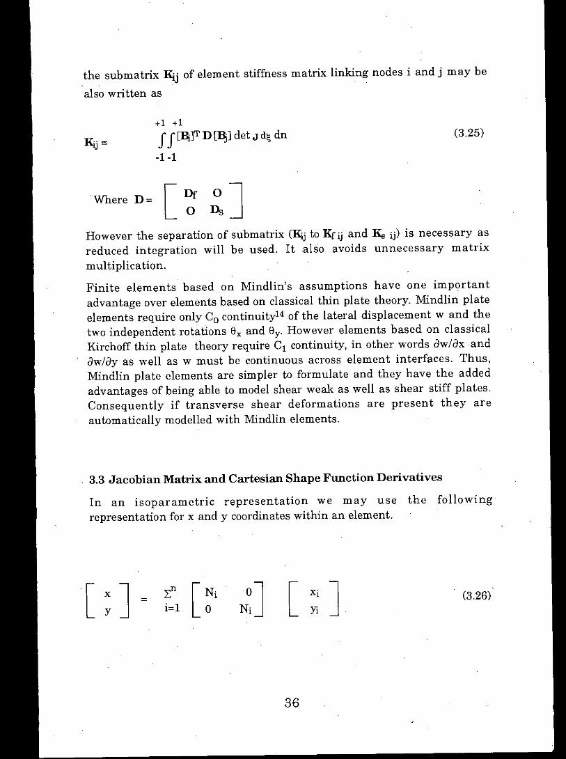
However the separation of submatrix (K;.j to Krij and lis ij) is necessary asreduced integration will be used. It also avoids unnecessary matrixmultiplication.

Finite elements based on Mindlin's assumptions have one importantadvantage over elements based on classical thin plate theory. Mindlin plateelements require only Co continuity14 of the lateral displacement wand thetwo independent rotations Sx and Sy. However elements based on classicalKirchoff thin plate theory require C1 continuity, in other words aw/ax. andaw/ay as well as w must be continuous across element interfaces. Thus,Mindlin plate elements are simpler to formulate and they have the addedadvantages of being able to model shear weak as well as shear stiff plates.Consequently if transverse shear deformations are present they areautomatically modelled with Mindlin elements.

[ ; J =

37

(3.31)

(3.30)

(3.29)

-1 a~ <1l'] ay ay

J = ax ax 1 <1l'] a~ (3.28)---a~ <1l'] detJ ax ax

ay ay <1l'] a~

in which Ni depend on the special coordinates and are known collectively asthe shape functions matrices.

The initial step of any finite element analysis is the unique description ofthe unknown function u (in our case the displacement field) within eachelement in terms of n parameters <1;.

3.4 Shape Function

aNi aNi a~ aNi <1l']

ax = a~-+- axax <1l']

aNi aNi a~ aNi <1l']and ay = ay+a~ <1l'] ax

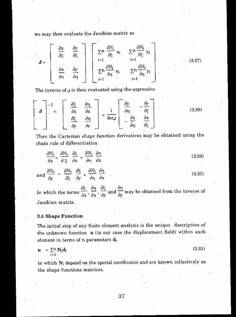
a~ <1l'] a~ <111 .In which the terms ax 'ax 'ay and ay may be obtained from the inverse of

Jacobian matrix.

Then the Cartesian shape function derivatives may be obtained using thechain rule of differentiation

ax ay aNi aN.2:n - n_'

a~ a~ a~ Xi 2: a~ Yi

J= i=l i=l (3.27)

ax ay aNi aNi2:n <1l'] Xi 2:n <1l'] Yi

<1l'] <1l'] i=l i=l

The inverse of J is then evatuated using the expression

we may then evaluate the Jacobian matrix as

With the displacements known at all points within the element, the strainsat any point can be determined by the relationship.E = ~nB;di (3.32)

i=l

where the strain matrix B; is generally composed of shape function

derivatives.

The efficiency of any particular element type used will depend on how wellthe shape functions are capable of representing the true displacement field.The choice of appropriate shape function is however not arbitrary and thereare two minimum conditions which must be satisfied in order to ensureconvergence of the solution to correct result as the finite element mesh is

refined:

Shape function must guarantee continuity of the function betweenelements (known as the continuity condition).

In the limit as the element size is reduced to infinitesimaldimensions, the shape function must be able to reproduce a c'onstantstrain condition through the element. Thus the unknown functionmust be able to take up in the limit any linear form throughout theelement (known as the constant strain condition).

The isoparametric family are a group of elements in which the shapefunction are used to define the geometry as well as the displacement field.In the present study three different element types considered are all basedon an isoparametric formulation. The elements included are illustrated inFig. 3.2 and are:

• The 4 noded bilinear element.

• The 8 noded serendipity quadrilateral element with a quadraticvariation of the displacement field.

• The heterosis quadrilateral element with quadratic Lagrangianinterpolation for ex and ey and quadratic serendipity interpolation for

w.

38

Recent research indicates that15 the use of a 'Heterosis' quadrilateralMindlin plate element with quadratic Lagrangian interpolation for Hx and

Shape Functions Local Coordinates

4 noded element: Local node number ~. 111. 1

NL(1;,11)= (1+1;1;i)(1+11TJi)14 4 noded el. : 1 -1 -1

i = 1, 2, 3 and 4. 2 1 -1

8 noded element: 3 1 1

• for comer nodes 4 -1 1

Ni(1;,11)=(l+1;1;i)(1+1111i)(1;1;i+1111i-1)14 8 noded el.: 1 -1 -1

i = 1,3,5,7 2 0 -11;2.1 .

• for midside node N;(1;,11)=T(l+1;1;i) 3 1 -1

11.2(1-112)++(1+1111i)(1-1;2), i = 2,4,6,8. 4 1 0

heterosis element: 5 1 1

• the first 8 shape functions are borrowed 6 0 1

from 8 noded element 7 -1 1

• for the control 9th node 8 -1 0

ng (1;,11)= (1-1;2)(1-112) and so on.

5

3

4

9

2

o

6

8

1

7

(c) heterosis element

5

3

4

2

6

1

8

7

(b) 8 noded element

2

39

3

Figure 3.2 Different Mindlin plate elements with respective

shape functions.

1

4

(a) 4 noded element

By and quadratic serendipity interpolation for w together with selectiveintegration of the stiffness matrix, gives the best overall performance. Itavoids locking and contains no spurious mechanisms. The Heterosiselement is implemented here using a hierarchical formulation.

3.4.1 Hierarchical Formulation of the Heterosis Element

In the implementation of the heterosis element a hierarchical formulationis adopted. The first 8 shape functions are borrowed from the 8 nodedserendipity element and the shape function for the central 9th node is the

bubble functionN9C1;,1'])= (1-s2) (1-1']2) (3.33)

which is available from the quadratic Lograngian element. This meansthat all variables associated with the central node are hierarchical innature. In other words, they are departures from the interpolatedserendipity values. The hierarchical representation can be used forgeometrical representation as well as for interpolating displacements.

In order to implement the heterosis element a hierarchical formulation canbe adopted either by adding a stiff spring (large number) to the leadingdiagonal term of the stiffness matrix associated with the lateraldisplacement parameter for node 9, or by prescribing displacement at thiscentre node to zero. This has the effect of forcing w to behave as though itwas represented by serendipity quadratic shape functions. Thus the desired

effect is achieved.

It is worth noting that if no spring is added the element obtained is identicalto the 9 noded Lagrangian element provided that care is taken in evaluatingthe consistent nodal forces. Furthermore if stiff springs are added to all theterms of the leading diagonal associated with node 9, then the elementreverts to a serendipity 8 noded element.

For convenience, in the present case, when representing the geometry ofthe heterosis element, the x and y coordinate departures from theinterpolated serendipity values are taken as equal to zero. In other words,as serendipity geometrical representation is adopted this distinction is onlyof importance when elements with curved boundaries are present.

40

41

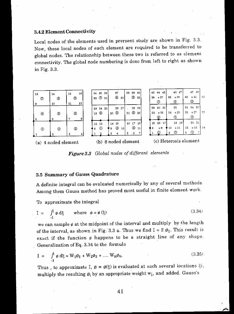
3.4.2 Element Connectivity

14

25

(c)Heterosis element

43 44 45 46 47 48 4936 037 36 039 40 041

(J) @ @

29 30 31 32 33 34 35

22 023 24 025 26 027

@ @ @

15 16 17 18 19 20 216 09 10 011 12 0131 CD 3 (1) 5 @ 7

(b) 8 noded element

34 35 36 37 38 39 40

30 (J) 31 @ 32 @ 33

23 24 25 26 27 28 29

'19 @) 20 @ 21 @ 22

12 13 14 15 16 17 18

8 (j) 9 (1) 10 @ 111 2 3 4 5 6 7

Figure 3.3 Global nodes of different elements

I = f ~dl; where ~ = ~ (1;) (3.34)-1

we can sample ~ at the midpoint of the interval and multiply by the lengthofthe interval, as shown in Fig. 3.3 a. Thus we find I '" 2 01' This result isexact if the function ~ happens to be a straight line of any shape.Generalization ofEq. 3.34 to the formula

I = f ~dl; '" W101 + W202 + .... Wn0n. (3.35)-1

Thus, to approximate I, 0 = 0(1;)is evaluated at each several locations 1;i,multiply the resulting 0i by an appropriate weight Wi, and added. Gauss's

To approximate the integral

A definite integral can be evaluated numerically by any of several methods.Among them Gauss method has proved most useful in finite element work.

3.5 Summary of Gauss Quadrature

13 14 15 16(J) @ @

9 10 11 12

@) @ @

5 6 7 8

(j) (1) @

1 2 3 4

(a) 4 noded element

Local nodes of the elements used in prersent study are shown in Fig. 3.3.Now, these local nodes of each element are required to be transferred toglobal nodes. The relationship between these two is referred to as elementconnectivity. The global node numbering is done from left to right as shown

in Fig. 3.3.

(3.36)

+1

"

(c)Three point

- 1+1

"

(b) Two point

- 1+1

"

Order Location 1;i Weight Wi "

1 0.000000000000000 2.000000000000000

2 ":1:0.577350269189626 1.000000000000000

.3 :1:0.774596669241483 0.5555555555555560.000000000000000 0.888888888888889

(a) one point

-1

In computer work numerical data for 1;i and Wi should be written with as

many digits as the machine allows.

Table3.1 Sampling Points and Weights for Gauss Quadratue

42

In two dimensions we find quadratue formula for 0 = 0(1;)by integratingwith respect to 1;and then with respect to 'Yj.

f1f1 f" 1 +1I = "0(1;,'Yj)d1;d'Yj",' [L wi 0(1;i,'Yj)d'Yj.1 -1 .1 i = .1

I", (1.0)(0 at 1;= - 0.57735 ...) + (1.0)(0 at 1;= + 0.57735)

Sampling points are located symmetrically with respect to the centre of theinterval. Symmetrically paired points have the same weight wi. The

following Table 3.1 give data for Gauss rules of order n = 1 through n = 3.For an example application, considering n=2 and Eq 2.35 we find

method locates the sampling points so that for a given number of them,greatest accuracy is achieved.

.Figure3.4 Qualitative representation of Gauss quadrature for differentnumber of sampling points:

43

(3.37)

"

5L2{F} [Kj, + K,,] {a}

= . [12(1 + v )]h2

In recent years several efficient plate bending elements have been reportedin the literature. Among these, plate bending elements which are based onMindlin plate theory and reduced integration are foundI6 to be extremelyeffective and efficient in application. However the main problem with theseelements is that they can suffer from shear locking as the thickness tolength ratio becomes small. Various methods can be used to alleviate thisproblem, the most common of which is the use of reduced integrationI6.However reduced integration has to be used with care, since spurious zeroenergy or modes or 'mechanisms' can occur, and the performance of the.elements can deteriorate when they are distorted. A zero-energydeformation mode arises when a pattern of nodal d.o.f produces a strainfield that is zero at all quadrature points.

where v is the poison's ratio of the plate material, h is the plate thickness,Kj, and K" are the stiffness due to bending and shear deformation,respectively and L is a reference length (e.g length or.width) of the plate.

For a thin plate L2/h2 -+ 00. To obtain a proper solution for Eq. 3.37 undersuch conditions K" should be singular, .otherwise shear deformationdominate and the system will be overstrained. The technique of reducedintegration ensures the singularity of K" and a proper solution of Eq. 3.37 isobtained over the 'thin plate' range. However it should be ensured that thetotal stiffness matrix [Kj, +K,,[(5L2/12(1 + v)h2] is non - singular.

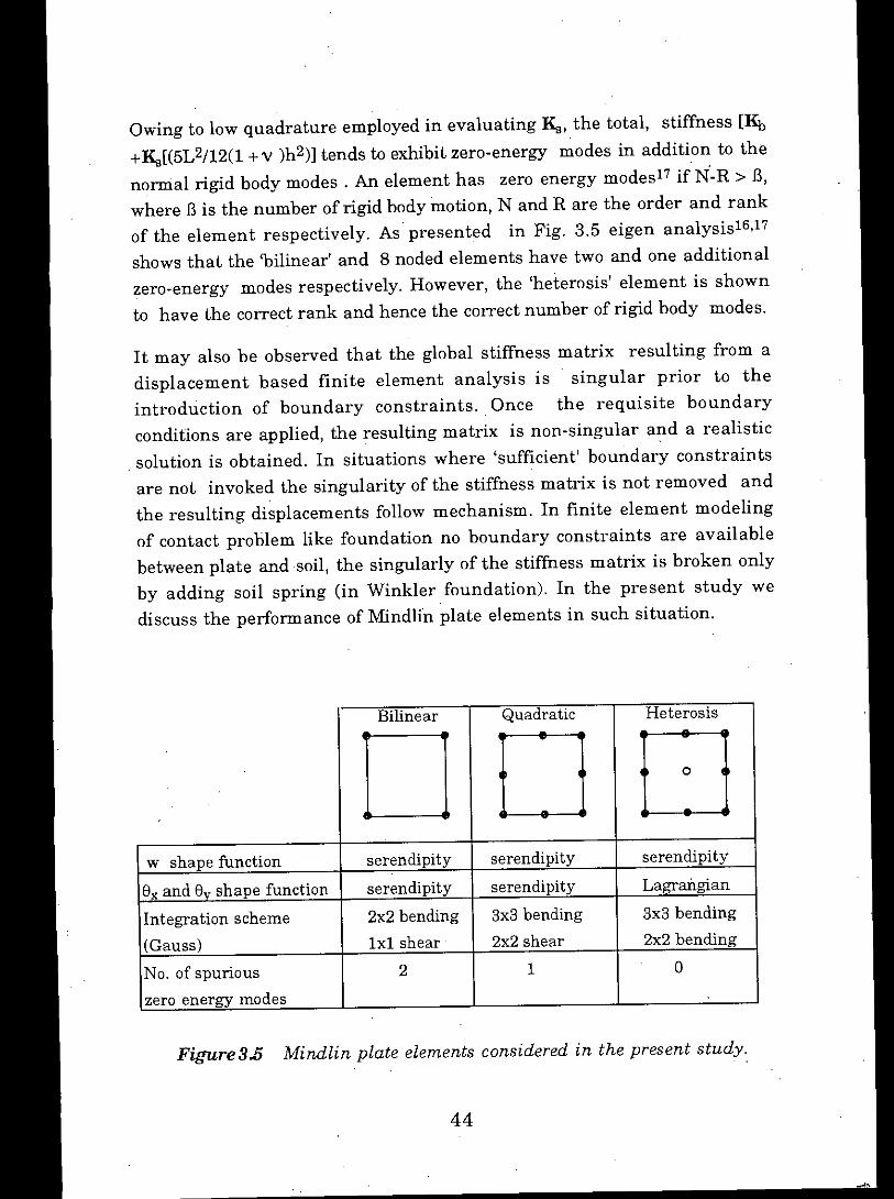
The three different plate bending elements viz. 'bilinear', 'quadratic' and'heterosis' considered in the present study are based on the theory ofMindlin plates. The major. characteristics of these elements aresummarized in the Fig. 3.5. It may be shownI6 that the formulation basedon the Mindlin's plate theory leads to a system of equations of the form,

3.5.1 Appropriate Order of Quadrature

It is not necessary to use the same number of Gauss points In eachdirection, but this is most common.

Owing to low quadrature employed in evaluating 1\". the total. stiffness [Kj,

+1\,,[(50/12(1 +v )h2)] tends to exhibit zero-energy modes in addition to thenormal rigid body modes. An element has zero energy modes1? if N-R > fl.where fI is the number of rigid body motion. Nand R are the order and rankof the element respectively. As presented in Fig. 3.5 eigen analysis16,1?shows that the 'bilinear' and 8 noded elements have two and one additionalzero-energy modes respectively. However, the 'heterosis' element is shownto have the correct rank and hence the COITectnumber of rigid body modes.

It may also be observed that the global stiffness matrix resulting from adisplacement based finite element analysis is singular prior to theintroduction of boundary constraints .. Once the requisite boundaryconditions are applied, the resulting matrix is non-singular and a realistic. solution is obtained. In situations where 'sufficient' boundary constraintsare not invoked the singularity of the stiffness matrix is not removed andthe resulting displacements follow mechanism. In finite element modelingof contact problem like foundation no boundary constraints are availablebetween plate and soil, the singularly of the stiffness matrix is broken onlyby adding soil spring (in Winkler foundation). In the present study wediscuss the performance of Mindlin plate elements in such situation.

Bilinear Quadratic Heterosis

D D Dw shape function serendipity serendipity serendipity

8x and 8v shape function serendipity serendipity Lagrangian

Integration scheme 2x2bending 3x3bending 3x3bending

(Gauss) Ixi shear 2x2 shear 2x2bending

No. of spurious 2 I 0

zero energy modes

Figure8.5 Mindlin plate elements considered in the present study.

44

I"'~--------------, ', ', ', ', ', ', '

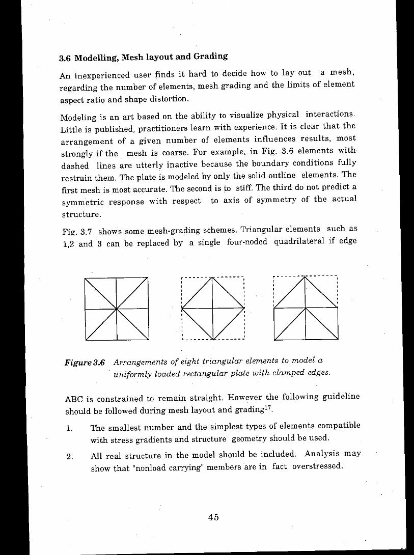
Figure3.6 Arrangements of eight triangular elements to model a. uniformly loaded rectangular plate with clamped edges.

ABC is constrained to remain straight. However the following guidelineshould be followed during mesh layout and grading17.

1. The smallest number and the simplest types of elements compatiblewith stress gradients and structure geometry should be used.

2. All real structure in the model should be included. Analysis mayshow that "nonload carrying" members are in fact overstressed.

45

Fig. 3.7 shows some mesh-grading schemes. Triangular elements such as1,2 and 3 can be replaced by a single four-noded quadrilateral if edge

An inexperienced user finds it hard to decide how to layout a mesh,regarding the number of elements, mesh grading and the limits of element

aspect ratio and shape distortion.

Modeling is an art based on the ability to visualize physical interactions.Little is published, practitioners learn with experience. It is clear that thearrangement of a given number of elements influences results, moststrongly if the mesh is coarse. For example, in Fig. 3.6 elements withdashed lines are utterly inactive because the boundary conditions fullyrestrain them. The plate is modeled by only the solid outline elements. Thefirst mesh is most accurate. The second is to stiff. The third do not predict asymmetric response with respect to axis of symmetry of the actual

structure.

3.6 Modelling, Mesh layout and Grading

46

,

A

E2

'3

Figure.3.7 Some coarse mesh to fine-mesh transition schemes,

c

These items are only suggestions and for each one there may be animportant exception.

6. The mesh layout is probably adequate if alterations do little'to change

the results.

7. Only if computed displacements are deemed agreeable shouldcomputed stresses be taken seriously. However, a mesh that givesgood displacements may be too course to yield accurate stresses.

3. When possible element boundaries should be aligned with structuremembers and with principal loading trajectories.

4, Element aspect ratios should not exceed roughly 7 for gooddisplacement results and roughly 3 for good stresses results.

5. Mesh grading should be done in such a way that abrupt, changes inelement size are minimized,

3.7 Soil ParameterIn the present study the soil under the foundation is considered as Winklermedium and modulus .ofsubgrade reaction concept is used. In the followingsections different approches for determination modulus of sub gradereaction and node springs are described ..

3.7.1Modulus of Sub grade Reaction

The modulus of subgrade reaction is a conceptual relationship between soilpressure and deflection that is widely used in the structural analysis offoundation members. It is used for footings, mats and various types ofpilings. The basic equation when using plate-load test data is

qk =_ (3.38)s 1\

where ks '= modulus of subgrade reactionq = soil pressure1\= deflection

Plot of q versus 1\from load tests gives curves of the type qualitatively shownin Fig. 3.8b. If this type of curve is used to obtain ks in the above equation, itis evident that the value depends on whether it is a tangent or secantmodulus and the location of the coordinates of q and 1\..

Obviously one could divide the q-1\curve into several regions so that ks takeson values of the slope in the several regions; however, this tends toincorporate too much refinement into the problem. Since most analysisproceed on the basis of estimated values or at best an approximate load test.

Fig. 3.8c is the idealisation of load-deflection curve proposed by Bowles sothat ks has a constant upto a deflection of xmax' Beyond Xmax the soilpressure is a constant value defined byq cont. = ks(Xmax) (3.39)

The value ofxmax may be directly extimated at some small value (say 12 to 25

mm) or from inspection of load settlement curve.

It is difficult to make a plate-load test4, except for very small plates becauseofthe reaction load required to achieve uniform displacement all over. Evenwith small plates of say 450, 600 or 750 mm diameter it is difficult to obtainuniform 1\since the plate tends to be less than rigid and constant deflection

47

Stacked plates

q

Non linear

Xmax

q' * q and Ii' = Iiif the plate is not rigid

q = PIA

----) b

(c)

t

q

I

b'

t(a)

q"

Load Block

t

ks = qlbks depends on curvecoordinates used and isgeneral!y non linear

) b

(b)

--------------------- --------------------

48

I/

I II I1/IIII1/

Figure 3.8 Determination of modulus of subgrade reaction ks'

q

1

across the plate (and definition of ks) is difficult to obtain . Stacking thesmaller plates concentric with the larger ones tends to increase therigidity. but in any case the plot is of load divided by plate contact area(nominal PIA) and the average measured deflection ..

The Road Research Laboratory18 uses the pressure corresponding to 0.13

em (0.05 in) obtaining

49 .

Since the twelfth root of any value x 0.65 will be close to 1 for all practicalpurposes the Vesic equation reduces to

Esks = B( -Il 2) (3.47)

(3.46)

(3.44)

(3.43)

(3.40)qks = 0.13 Kg/ cU.m

Vesic20,21 proposed that the modulus of subgrade reaction could becomputed using the stress-strain modulus Es as

, 12-JEsB4 Es .ks = 0.65 EIf --2s 1-1l

where ks'= ksBEs,Ef= modulus of soil and footing respectiveiy in consistent unitB, If = footing width and its moment of inertia, in consistent unit.

For a rectangular footing on sand of dimensions B x'mB:

m+0.50ks = kl (3.45)

1.5m

In these equations ks = desired value for full-sized footing and k1 = valuefrom a lx1 ft square plate load test.

California Bearing (CBR) tests have also been used to obtain the subgrademodulus. The penetration load at 0.25 cm (0.1 in) corverted to pressure (loadper area, where area computed based on a piston diameter of 4.95 cm) yields

qCBRkg = 0.25 (3.42)

Terzaghi19 proposed that ks for full-sized footings could be obtained fromplate-load tests using the following equations:

For footing on clay:ks = k1B

For footing on sand (including size effects) :. B+l 2

ks = kl ( 2B )

The U.S Corps of Engineers has used the diformation corresponding to 0.7Kg/sq.m (10 Psi) for evaluation of subgrade for airfields as

0.7 .ks= ""6 Kg/cu.m (3.41)

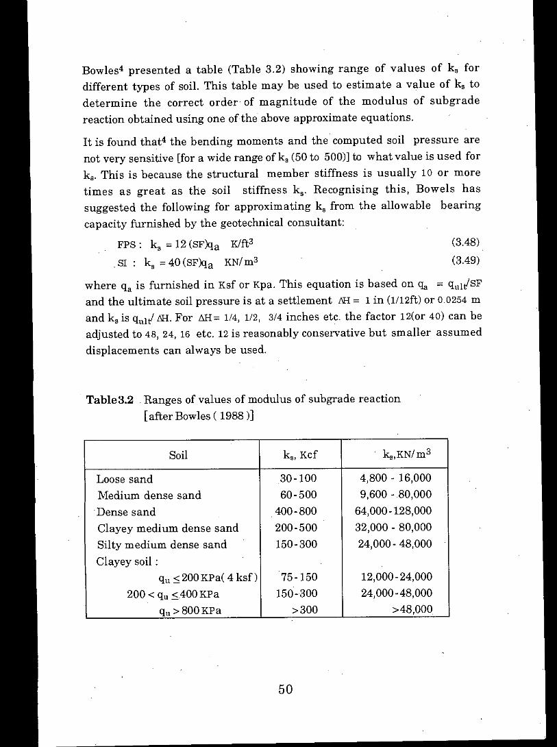
'Table3.2 Ranges of values of modulus of subgrade reaction[after Bowles ( 1988)]

Bowles4 presented a table (Table 3.2) showing range of values of k. fordifferent types of soil. This table may be used to estimate a value of k. todetermine the correct order of magnitude of the modulus of subgradereaction obtained using one of the above approximate equations.

(3.48)

(3.49)

k.,KN/m3

12,000-24,00024,000-48,000

>48,000

4,800 - 16,0009,600 -80,000

64,000-128,00032,000 - 80,00024,000- 48,000

k., Kcf

50

75-150150-300

>300

30-10060-500

,400-800200-500150-300

FPS: k. = 12 (SF)qa K/ft3

.S1 : k. = 40 (SF)qa KN/m3

Soil

Loose sandMedium dense sandDense sandClayey medium dense sandSilty medium dense sandClayey soil :

qu ~200KPa( 4 ksf)200 < qu ~400 KPa

qu>800KPa

where qa is furnished in Ksf or Kpa. This equation is based on ~ = qult"SFand the ultimate soil pressure is at a settlement &I = 1 in (1I12ft)or 0,0254mand k. is quIt"&I. For MI= 114,112, 3/4 inches etc. the factor 12(or 40) can beadjusted to 48, 24, 16 etc. 12is reasonably conservative but smaller assumeddisplacements can always be used.

It is found that4 the bending moments and the computed soil pressure arenot very sensitive [for a wide range of k. (50 to 500)] to what value is used fork•. This is because the structural member stiffness is usually 10 or moretimes as great as the soil stiffness k•. Recognising this, Bowels hassuggested the following for approximating k. from the allowable bearingcapacity furnished by the geotechnical consultant:

51

3.7.2 Evaluation of Node Spring From Modulus of Subgrade Reaction ks

abc

1 I 2 1.--r--- - -- -1---131

ci 1 elf--1_- ---1---

I I~

Contributing area:k,x 1/4 of rectangle abed (corner).k,x 1/4 of abed and 1/4 bcfek,x 1/4 each. rectangle with common

corner node (interior node)

Figure 3.10 Method of prorating ks to buildnode springs for 8 noded orheterosis element.

Figure 3.9 Method of prorating ks 10

build node springs for 4noded bilinear element.

From subgrade reaction k, the node springs can be computed either byusing shape function or it may be based on the contributing area of the plateto the node. When shape function is used the equivalent node springs willbe similar to equivalent nodal forces evaluated from distributed loading.When contributing area (Figs. 3.9 and 3.10) is used the equivalent nodesprings will be as follows:

4 noded bilinear element:

Node123

8 noded serendipity quadrilateralelement or heterosis element:

Node Contributing area " hI 2 -' ,

1 ksx 1/16 of rectangle abed 0 0 ,-~ , - -- !---------2 ksx 3/16 of rectangle abed ,./ --l - -, - -1/16 of abed and 1/16 of - r- - - -.' 'j- - - - - - - - -3 ksx - -,

J 0 , , 0

bcfe .< 00, ,- - -... .. ..- - - - - - - - -4 ksx 3/16 of abed and 3/16 of . , .:..•..••....••,

- -0 >-- - - -. ... - - - -bcfe and so on. 0 ,0 0

4,000 KJ'Ilm

-5333.33 KN/m

,

12,000 KNlm

21333.33 KN/m

"

2in

i

,

i

2m

,

4,000 KN/m

ks = 16,000 KNhn3

\ - •..•.ks = -'-i6 000 KN/m3.... , ,- ,,,

i

.,,

2m

2m

i i4,000 KJ'I/m 12,000 KN/m

52

(a) Using shape function.

(b)Using lumped method

-5333.33 KJ'I/m 21333.33 KJ'ilm -5333.33 KJ'I/m

Evidently when 4 noded bilinear element is considered both shape functionand lumped method gives identical node springs. Thus for 4 noded elementnodal spring values will be computed using shape function only. When 8noded or heterosis element is considered the node springs will similar asshown in Fig. 3.11. As mentioned earlier, the nodal springs will havedifferent values for 8 noded or heterosis plate elements based on whether thecomputation is made using lumped method or shape functions. This isexplained with an example plate element of size 2m x 2m and soil ks = 16,000KN/ m3 and resulting spring values are shown in Fig. 3.11.

Figure3.11 Equivalent node springs computed from subgrade reaction.

From Fig. 3.11a it is seen that in order to obtain a uniform settlementcorner nodes need to be held down to avoid soil-footing separation. As soiltension is not permitted, this means when shape function is used, thesystem will be consistent as long as there is no soil separation. Thus whensoil separation occurs, option two, lumped method is desirable. It is alsoexpected that for fine mesh without soil separation both shape function andlumped methods will provide almost identical results .

.The system of soil springs described above is termed a "Winkler"foundation and the springs are uncoupled (though when shape function isused there is some coupling effect) Uncoupling means that the deflection ofany springs is not influenced by adjacent springs. Because the springs areuncoupled, some designers do not like to use the concept of ks, preferringinstead to use a FEM of elastic continuum with Es and Jl as elasticparameter. However the computations are extensive and only as good asone is able to estimate Es and Jl. In any case the use of ks in analysing matsis rather wide spread because of the greater convenience of this parameter.

Bowles4 has described a method to couple the springs to a limited extent. Ingeneral, coupling can be achieved as follows:

1. Doubling the edge springs of a mat. This is a first approximation.

2. The mat area can be divided into different zones and softer springsmay be used in the centre than at the edge and intermediate zonesmay be conceived from the edge to the centre forming the transition.

If option 2 is chosen, it is not usually necessary to use more than aboutthree zones, an edge, an intermediate, and a central zone of about onequarter of the mat area.

3.7.3 Soil Separation Consideration

The concept of subgrade reaction with spring contribution at nodes is easyto modify for soil separation, since the diagonal term (not all) is the only co-efficient in the stiffness matrix with the soil spring Ki

(Ali + Ki)Xi = Pi (3.58)Thus for soil footing separation we simply make Ki = 0, rebuild (or reuse acopy oDthe stiffness matrix, and again solve for the displacement xi.

53

(3.50)(3.51)

to the

3.7.4 Modulus of Subgrade Reaction and Consolidation Settlements

It is not uncommon that a mat is placed on a soil which is analysed byusing ks, but there are, in addition, consolidation settlements which willoccur later.

It is a relatively simple exercise in using the definition of ks to include theeffect of consolidation settlement, since the base contact pressure CJo remamconstant,

q" = ks &I = ks' (t.H + &Ie)

k; = (ks &I)/(&I + &Ie)

we can see that including the consolidation settlement reduces kslesser k;.

3.7.5 Consideration for Pile Foundation

Pile cap moment and shears for design are best obtained using a finiteelement or finite grid computer program. In the present study finiteelement method is used and in using the program one should add thefollowing pile springs (vertical as well rotational) at the nodes where thepile are located :

Kw = ks x contributing area + Al AEIL

4ElyKllx = A2 L

4ElxKey = A3-r-

where Kw is the equivalent vertical stiffness of the pile and soil springs Kllx

and Key are the rotational stiffness of pile in the x and y directionrespectively. E = modulus of elasticity, L = pile length (total including anypart not embedded, AI, A2 and A3 are the correction factors and depend thesoil characteristics and pile type. For friction piles Al = 2.0 to 1.0, while forpoint piles A] =1.2 to 1.1. AZ • AJ = 1.0 to 3.0; 1.0 for point piles where othervalue is for friction piles.

54

Chapter 4

COMPUTER IMPLEMENTATION

4.1 General.

The Mindlin plate formulation and basic procedures for analys(s offoundation described in the previous chapter have to transformed into acomputer program in order to study the analytical response of foundation.One of the primary objectives of this work was to develop a special purposeprogram capable of analysing different types of footings and matfoundation. Leaving aside all the theoretical aspects, the practical computerimplementation schemes adopted will be projected in the following sectionsof this chapter.

4.2 Overall Program Structure

The overall program structure for Mindlin plate bending analysis programMINDLIN using a non-layered approach is given in Fig. 4.1.

The dimension given in subroutine FEMATF agree with those given Insubroutine DIMMP and limit of the program to the following maximumsize problems in the present form.

MELEM maximum number of elements 100MEVAB maximum number of variables per element = 'XlMFRON maximum front width = 200MMATS maximum number of material sets = 10MPOIN maximum number of nodal points = 500MTOTV maximum total number of degrees of freedom = 5OOx3MVFIX maximum number of prescribed boundary nodes = 500

To modify these values the DIMENSION statements in FEMP and theappropriate statements. in DIMMP should be earefully changed andchecked. All routines are now documented and these include:DIMMP,INPUT, CHECK1, NODEXY, GAUSS,CHECK2, ECHO, ZEROMP,MINDPB, LOADPB, SFR2, JACOB2,INCREM, ALGOR, STIFMP, MODPB,BMATPB, SUBMP, FRONT, RESMP, GRADMP, STRMP, VZERO, OUTMP,SMOTH.

55

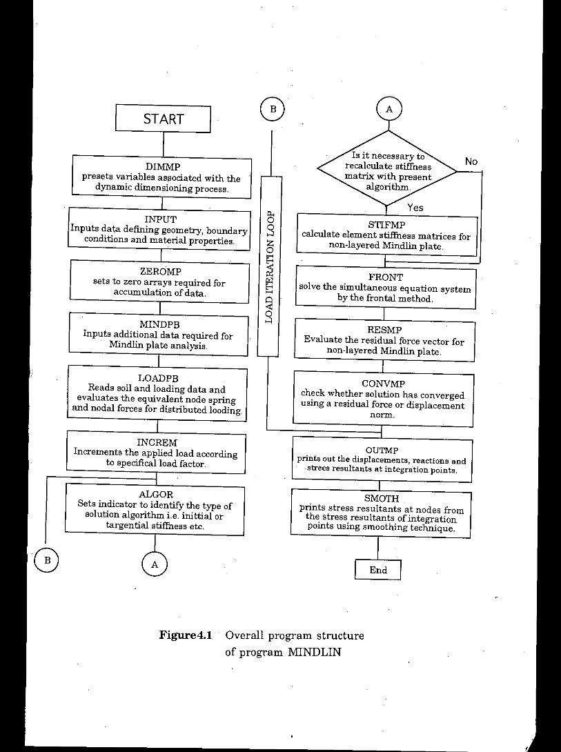
No

STIFMPcalculate element stifihess matrices for

non-layered Mindlin plate.

CONVMPcheck whether solution has convergedusing a residual force or displacement

norm.

RESMPEvaluate the residual force vector for

non-layered Mindlin plate.

SMOTHprints stress resultants at nodes fromthe stress resultants of integrationpoints using smoothing technique.

FRONTsolve the simultaneous equation system

by the frontal method.

OUTMPprints out the displacements, reactions and-strees resultants at integration points.

Figure4.1 Overall program structureof program :MINDLIN

START

DIMMPpresets variables associated with thedynamic dimensioning process.

IINPUT

Inputs data defining geometry, boundaryconditions and material properties.

IZEROMP

sets to zero arrays required foraccumulation of data.

MINDPBInputs additional data required for

Mindlin plate analysis.

ILOADPB

Reads soil and loading data andevaluates the equivalent node springand nodal forces for distributed looding.

INCREMIncrements the applied load according

to specificalload factor.

ALGORSets indicator to identify the type ofsolution algorithm i.e. inittial or

targential stifihess etc.

B 8

4.3.2 Subroutine DIMMP

4.3.3 Subroutine INPUT

total number of nodal points in the structuretotal number of elements in the structuretotal number of boundary nodesnumber of nodes per elementtotal number of different materials in the structurethe order of Gaussian quadrature rule to be employed fornumerical integration.

parameter controlling reduced integration and full integration.For example NGAUS equals to 3 andINTEP equals to 0 means a :Jpoint Gauss rule to be employed for bending and a 2 point rule forshear. On the other hand ifNGAUS equals to 3 and INTEP equalsto 1, a 3 point rule to be employed for both bending and shear

57

4.3 Brief Description of Modular Routines

The overall computational procedure adopted here is accomplished throughthe various subroutines given in the general flow diagram of Fig. 4.1.A brief description of the operational functions achieved in these routinesare furnished below.

4.3.1 Subroutine FEMATF

The channel numbers 'used for input files and output files (line printer) are5 and 6 respectively. Channel numbers 1,2;3,4 and 8 are also used to createscratch files during program execution.

This routine controls the calling sequence of 'all other main routines asindicated in Fig. 4.1.

The role of this subroutine is to accept most of the input data. The controlparameters necessary for two dimensional applications particularly forplate bending problem are presented below.

NPOINNELEMNVFIXNNODENMATSNGAUS

INTEP

This subroutine sets up the dimensions which must agree with the size or. the arrays in subroutine FEMP ..

IRAFT special problem Type parametero - slab problem1- foundation problem, where soil separation is considered.2- foundation problem, where soil separation is not allowed.

NALGO parameter controlling solution algorithm:1- initial stiffness method. The element stiffness are computed at

the beginning of the analysis and remain unchanged thereafter.2 ' tangent stiffness method. The element stiffness are recomputed

during each iteration of each load increment.

For foundation problem parameter 2 is essential. Because, as soil tension isnot permitted, when soil separation occurs it is necessary to recalculateelement stiffness matrices. However parameter 1 may be used where soilseparation does not occur.

For the present two dimensional applications two co-ordinate componentsare required to locate each nodal point. This information is stored in thearray COORD(IPOIN, IDIME) where IPOIN corresponds to the number ofthe nodal point and IDIME refers to the co-ordinate components. Mid-sidenodes of 8 and 9-noded elements need not be supplied if they lie on a straightline between corner nodes. The co-ordinates of such intermediate nodes are.evaluated by subroutine NODEXY by linear interpolation.

For each nodal point at which displacement value corresponding to one 0'.

more degrees of freedom are prescribed, input data supplied specifyingthese fixity conditions are stored in the array.

NOFIX(IVFIX)

which signifies that the IVFIXth boundary node has a nodal point numberNOFIX(IVFIX). Input parameter IFPRE controls which .degrees of freedomof a particular node are to have a specified displacement value, Forexample, integer code IFPRE may have the following values:

010 - displacement in the x direction specified.001.~ displacement in the y direction specified.011 - displacement in both x and y directions specified.111 - displacement in both x and y directions as well as III the z

direction specified.

This information is then transferred, for permanent storage into array.

58

IFFIX (lTOTV)where ITOTV ranges over the total number of degrees of freedom of thestructure. The prescribed displacement value associated with a restraineddegree of freedom is stored in array,

PRESC(lVFIX,IDOFN)

where IVFIX indicates that the prescribed displacements pertain to the

IVFIXth boundary node and IDOFN ranges over 'the degrees of freedom ofthat node.

For two-dimensional application particularly for plate bending problem thefollowing material parameters' must be input

PROPS(NUMAT,l) Elastic modulus, EPROPS(NUMAT,2) - Poison's ratio, vPROPS(NUMAT,B) - Material thickness, tPROPS(NUMAT,4) - Material mass density, pconsequently NPROP = 4.

Subroutine INPUT also calls subroutine' GAUSS described in sec. 4.8.;:;whose function is to generate the sampling point position and weightingfactors for numerical integration.Subroutine INPUT is now self-explanatory.

4.3.4 Subroutine NODEXY

This subroutines evaluates midside nodes for straight sided 8 noded andheterosis elements. This routine also evaluate the co-ordinates of the centralnode. Here a hierarchical formulation is chosen and the values at thecentral node and the departures from the interpolated serendipity valuesare always taken as zero.

4.3.5 Subroutine GAUSS

The function of this subroutine is to set up the sampling point positions andweighting factors for numerical integration. The Gauss quadratrue processutilized here are restricted to one, two and three point integration rules. Theorder of integration rule to be employed is defined by NGAUS and INTEP.

59

The sampling point positions and weighting factors are stored respectivelyin arrays POSGP( ) and WEIGP( ).

4.3.6 Subroutine SFR2

The role of this subroutine is to evaluate the shape functions Ni(S,'I) andtheir derivatives aNi/as, aNi/drj at any sampling point (Sp,lIp) within theelement for each of the 4-, 8- or 9~noded elements as described in sec. 3.4.The sampling point co-ordinates sP'llp are specified as EXISP and ETASPrespectively. The evaluated shape functions for each node of an element arestored in array SHAPE (NODE) and derivatives in array DERIV(INODE,IDlME) where INODE ranges over the element nodes and IDlME over theco-ordinate dimensions.

4.3.7 Subroutine JACOB2

This subroutines calculates for any sampling position (sp' '1pJ (usually theGauss point) the following quantities:

• The Cartesian co-ordinates of the Gauss point which al'estored in the array GPCOD( ).

• The Jacobian matrix which are stored in XJACM ( ). TheJacobian matrix is defined by equation Eq.3.27

• The determinant of the Jacobian matrix, DJACB• The inverse of Jacobian matrix, is stored as XJACI( )• The Cartesian derivatives aNi/ax. aNi/ay of the element shape

functions. These quantities are defined in Eq. 3.29 and Eq. 3.:30.

4.3.8 Subroutine CHECKl

The function of the subroutine IS to scrutinise the problem controlparameters which are accepted by the data input subroutine, INPUT.Subroutine CHECK1 will check that the control parameters are within thebounds defined by the correct values for plate bending application.

A counter,'KEROR is employed to indicate whether or not any errors havebeen detected. If errors have been found (indicated by KEROR =0 1 I,

subroutine ECHO described in sec. 4.3.10 is called to list the remainder ofthe input data.

60

Errors detected are signaled by means of printed error numbers from 1 to 9.

4.3.9 SubroutineCHECK2

If the problem control parameters have passed the scrutiny of subroutineCHECK1, the geometric data, boundary conditions and material propertiesare then assimilated by subroutine INPUT. This data is then scrutinized fOl'possible errors in subroutine CHECK2 where error types 10 to 21 arechecked for.

Probably the most useful check in this subroutine is the one which ensuresthat the maximum front width does not exceed the dimensions specified inthe subroutine FRONT.

4.3.10 Subroutine ECHO

The function of this subroutine is to list all the remaining data cards after atleast one error has been detected by either of the diagnosis subroutinesCHECK1 or CHECK2. This is accomplished by means of a simple read andwrite operation in alphanumeric format.

4.3.11 Subroutine ZEROMP and VZERO

These routines simply set to zero the components of various vectors andarrays.

4.3.12 Subroutine MINPB

This subroutine simply reads some additional information required forcontrolling the convergence check and inserting additional constraints forthe Heterosis element.

4.3.13 Subroutine LOADPB

The role of this subroutine is to evaluate the consistent nodal forces for eachelement. It is also capable to evaluate node springs from subgrade 01' pilereactions for foundation type problems.

For plate bending applications two forms of loading are considered. Firstlyload components corresponding to the permissible generalized forces (i.e. aload in the z direction and couples acting in both xz and yz planes) may be

61

62

4.3.14 Subroutine ALGOR

controls application of point spring(spring directly applied atnodes).o - no point springs are applied1 - point springs are read as inputcontrols the application modulus of subgrade reactiono - modulus of subgrade reaction is absent.1 - node springs are evaluated from subgrade reaction by using

shape function

2 - node springs evaluated from subgrade reaction is based oncontributing area method.

IPSPR

MSUBR

As mentioned above there is provision in the subroutine for calculation ofnode springs. The procedure similar to load calculation. The followingparameters are used to control such application.

prescribed at the nodal points. Secondly a uniformly distributed load actingnormal to the plate may be applied. A parameter IPLOD controls theapplication of point load. If parameter IPLOD is non zero the applied nodalloads are read as input. For each particular node the applied point fOl'cesare associated with anyone of the elements attached to it, since eachelement contribution will be assembled before equation solution. Theconsistent nodal loads are evaluated for each element separately and stol'edin the array RLOAD(IELEM, lEVAB) where IELEM indicates the elementand lEVAB ranges over the degrees of freedom of the element.

The node springs thus evaluated are stored III the alTaySPLOD(IELEM,LEVAB). It is then transferred to subroutine STIFMP andadded with appropriate diagonal elements of the element stiffness matl'ices.

The function of this subroutine is to control the solution process accOl'ding tothe value of the solution algorithm parameter, NALGO, input in thesubroutine INPUT. The subroutine sets the value of indicator KRESL toeither lor' 2 according to NALGO and the current values of the iterationnumber IITER and increment number IINeS. A value of KRESL = 1indicates reformulation of the element stiffness accompanied by a fullequation solution and KRESL = 2 indicates that the element stiffness al'e notto be modified and consequently only equation resolution takes place.

4.3.15 Subroutine lNeREM

63

This controls the magnitude of the load increment. The appliedloading for each element is evaluated in the Subl'OutineLOADPB and stored in the array RLOAD(IELEM, IEVAB) asdescribed in section 4.16. The additional element load appliedduring the increment is RLOAD(IELEM,IEVAB) '> FACTO.The applied loading is accumulative so that if FACTO is inputas 0.8, 0.2 and 0.1 for the first three increments, the total loadacting on the structure during the 3rd load increment is 1.1times the loads calculated in the subroutine LOADPB. In thepresent study the total load is applied at a time consequent b~'FACTO=1.0.

This controls the tolerance permitted on' the convergence

FACTO

TOLER

The role of subroutine INCREM is to increment the applied loading or anyprescribed displacements according. to the load factors specified as input.This subroutine is accessed on the first iteration of each load increment. Foreach increment of load the following items of information are input as data.

process.

MITER Maximum permissible number of iterations. This is a safetymeasure to converses situations where the solution processdoes not converge. After performing MITER iteration cycle theprogram will then stop.

NOUTP(I) This parameter controls the output of the unconvergedresults after the first interaction.

NOUTP(2) This parameter controls the output of the converged l'esults ..For both NOUTP(l) and NOUTP(2) the following codes areusedo No print required1 print the displacements2 - print the displacements and nodal reactions3 - print the displacements, reactions and stresses.

The loading to which the structure is subjected is monitored by the arraysELOAD(IELEM, LEVAB) and TLOAD(IELEM,IEVAB). The total loadingapplied to the structure at any stage of the analysis is accumulated in theTLOAD array. On the other hand ELOAD contains the loading to be applied

to the structure for each interaction of the solution process. Initially (thefirst iteration of the first load increment) ELOAD contains the firstincrement of the applied load. For the second and subsequent iterationsELOAD contains the residual nodal forces. After convergence has occUlTed,the next increment of load is assimilated into ELOAD, so that at this stageELOAD contains the new applied load increment together with any residualstill reaming after convergence of the solution for the previous loadincrement. These residual forces should be negligibly small if theconvergence tolerance factor, TOLER, is correctly chosen. However, sinceany residual forces are retained in ELOAD and applied as nodal forcesduring next load increment, it is noted that equilibrium is maintained atevery stage of the computation process.

The final role of this subroutine is to insert appropriate values in the fixityarray to control any prescribed displacements. In order to arrive at thecorrect value of a displacement whose value is prescribed for a loadincrement, it is necessary to prescribe the given value for equation solutionduring the first iteration and then prescribe a zero value for all subsequentinteractions. Since the displacements occurring during each iterationaccumulate to give the total displacement then cli!arly the prescribed valuewill be obtained by this process. Subroutine INCREM is now self~explanatory.

4.3.16 Subroutine STIFMP

The purpose of this subroutine is to formulate the stiffness matrix for eachelemen,t. For foundation problem the soil springs evaluated by subroutineLOADPB are added with the appropriate diagonal terms of elementstiffness matrix and the data is stored on a disc file.

4.3.17 SubroutineMODPB

This subroutine evaluates the elasticity matrix Dfor plate bending situationaccordingto (3.5b). The result is partitioned into plane, DPLAN, flexUl'a!DFLEX and shear DSHER contributions.

64

4.3.18 Subroutine BMATPB

This subroutine evaluates the strain matrix B within any point of anelement for plate bending application according to (3.15). Again the Bmatrix is partitioned into plane, BPLAN, flexural, BFLEX, and shear,BSHER contributions.

4.3.19 Subroutine SUBMP

This subroutine evaluates [Bj]Tn (Bj]detJ x Gauss weights and is used lD

the evaluation of the element stiffness matrices.

4.3.20 Subroutine FRONT

The function of this subroutine is to assemble the contribution from eachelement to form the global stiffness matrix and global load vector and tosolve the resulting set of simultaneous equations by Gaussian directelimination. The main feature of the frontal solution technique is that itassembles the equations and 'eliminates the variables at the same time.Complete details ofthe frontal process can be found in Refs. 14 and 22.

4.3.21 Subroutine RESMP

The function of this subroutine is to evaluate the nodal forces which arestatically equivalent to the stress field. Comparison of these equivalent nodalforces with the applied loads gives the residual forces according to Eq. 3.18.As mentioned in the sec. 4.3.15, this residual forces are retained in thearray ELOAD and applied as nodal forces in the next iteration. This processis repeated till the convergence occurs.

The procedure adopted is as follows:

step a. The applied loads for rth iteration are the residual forces given

1j!r-l by Eq. 3.18 which give rise to displacement increments ddrand the strain increments dEr.

step b. The incremental stress changes are computed as' dur =DelEr

step c. The total stress for each element Gauss point is accumulated as

ar = ar-1+ dar where ar-1 are the converged stresses for r-1iteration

65

4.3.23 Subroutine STRMP

(411

(4 ..'3)

V[Lll(1jJi2)2i~l

---- x 100,;; TOLER (Force)V[Lll(J;r)2]i~l

---- x 100,;; TOLER (Disp.)v[L;ll(dir)2]i~l

step d. Finally the equivalent nodal forces from the element stresses arecalculated according to

66

'/Lll(0ir)2]i~l

This subroutine evaluates the bending moments and shear forces forMindlin plates.

This subroutine evaluates displacement gradients ow/ox, ow/oy, oHx/ux,oSxloy, aSy/ax and oSy/oy

4.3.22 Subroutine GRADMP

4.3.24 Subroutine CONVNP

This subroutine establishes whether a solution has conversed withreference to some displacement or residual force norm. That is we willassume that the numerical process has converged if

where n is the total number of nodal points in the problem and r denotes theiteration number. This criteria ,states that convergence occurs if the norm ofdisplacement change or residual forces becomes less than TOLER times thenorm of total conversed displacements or forces. In practical situations n

value of TOLER = 1.0 (i.e. 1%) is found to be adequate for the majority ofapplications14. Convergence of the solution is indicated by the parameter

NCHEK. A value of NCHEK = 1 indicates that convergence has not yetoccurred, whereas NCHEK = ° denotes a converged solution.4.3.25 Subroutine OUTMP

This subroutine outputs nodal displacements and reactions and also theGauss point stress resultants according to parameters NOUTPO) andNOUTP(2) as mentioned in the subroutine INCREMP.

4.3.26 Subroutine SMOTH

This subroutine evaluates stress resultants at nodes from Gauss pointstresses resultants using interpolation functions. Theoretical details isgiven in chapter 6. It has the following main parameters

S(I),T(l) elements local co-ordinatesCF(I,J) coefficient matrix ofEq. 6.9CS(I,J) coefficient matrix ofEq. 6.5A(l) coefficient ofEq. 6.6B(I) coefficient ofEq. 6.2STAEN(I,J) stresses at element node (local)NVALE nodal valenceASTRG(I,n average stresses of nodeSTAVP(IELEM) is very important parameter in this programme.

when averaging the stresses for any particulm'node, it controls the access of element stresses

STAVP(IEIEN) 0, element to be excluded during stress averaging1, element to be included duriJ;lg st1'essaveraging

67

Chapter 5

PERFORMANCE OF MINDLIN PLATEAND ITS CONVERGENCE

5.1 General

Convergence to exact answer will be approached as more and elements areused to model an arbitrary structure provided convergence requirements!7are satisfied. If there are enough time and money finer 'and finer meshcould be used to achieve the exact convergence. But from economic viewpoint, it is desirable to use optimum number of elements for practicalsolution. Moreover finite elements too converge in a perverse way : they.converge as the mesh is refined and then they diverse again because ofroundoff. Normally the mesh layout which produces the stresses of +2 to5% accuracy23 may be considered adequate. In this chapter, the formulationof Mindlin plate elements and its convergence are checked. In this studythe numerical factors a and 13 of simply supported square slab underuniformly distributed loading and concentrated loading are considered. Theeffect of plate thickness are also studied.

5.2 Square Slab Subjected to Uniformly Distributed Load

For uniformly loaded square plate the maximum deflection is given bywmax = a (qa4/D)

where q = uniformly distributed load on the plate.a = a numerical factor= 0.00406 for square plate24

a = plate dimensionD = Et3I[12(1. v 2)J

where E = modulus of elasticity of the plate materialt = plate thicknessv = poisons ratio

For Uniformly loaded square plate the maximum moment is given byMmax = Bqa2

with 13'= a numerical factor

= 0.0479 for square plate24with v = 0.30

68

5.3 Simply Supported Square Slab Subjected to Concentrated Load atCentre

For centrally loaded square plate the maximum deflection is given bywmax = a(Pa2/D)

where P = applied concentrated loada = plate dimensionD = Et3I[12(1 _v 2)]

a = a numerical factor= 0.01160 for square plate24

The maximum moment (in the vicinity ofthe load) is given by. Mmax = 13Pwith 13= 0.298

However the above 13values is valid when the load is applied over an area ofO.la diameter.

5.4 Comparison of Numerical Factors a and 13 for Uniformly LoadedSimply Supported Square Slab and Check for Convergence

Theoretical values24 of a and 13for uniformly loaded square slab are 0.00406and 0.0479 respectively. Using different mesh arrangements and slabthickness these theoretical values of a and 13are compared with those ofthick plate solution in Table 5.1 and 5.2 for different element types. Theconvergence of a and 13values is also examined in Figs. 5.1 and 5.2respectively. From Table 5.1 it is found that when the thickness of the slabused is 6 inches, a values obtained for 8 noded element and heterosiselement are about 2.0% greater than that of the theoretical value. This istrue for all mesh arrangements. From Fig. 5.1 it is observed that for 4 nodedelement the difference also approaches 2.0% as the mesh is refined. Inorder to study the effect of plate thickness on solution converge, slab havingthickness 3 inches is also considered for 8 noded element and heterosiselement, while other dimensions are not changed. It is found that a valuesare very close to the theoretical value for this thinner slabs. As shown inTable 5.1 the differences are only 0.5% for all mesh arrangements. Howeverfrom Table 5.2 and Fig. 5.2 it is observed that for all element types 13valuesobtained from thick plate solution is quite close to their theoretical value and

69

Table 5.1 Comparison of numerical factor a for uniformly loaded simply

supported square plate using one-quarter of the symmetric plate

Element Mesh Integratioa ••Wmaxj Theory+ %VariaType Arrange- D Scheme Wmaxft qa4m (qa4/D) "- tionment (Gauss)

"-2x2 0.003028 0.7454720 0.00406 0.00406 0--- --- --- ---4 noded 3x3 2x2 0.00306448 0.745720 0.00411 0.00406 1.2bilinear bending --- --- -.- ---element 5x5 Ixl shear 0.00308079 0.7454720 0.00413 0.00406 1.7-.- --- --- ---

2x2 0.00308623 0.745720 0.00414 0.00406 2.08 noded. --- --- -.- ---serendipity 3x3 3x3 0.00308917 0.7454720 0.00414 0.00406 20quadrila- bending 0.0243431* 5.963776* 0.00408* 0.5*teral 5x5 2x2 shear 0.00308954 0.7454720 0.00414 0.00406 2.0element 0.0243460* 5.963776* 0.00408* 0.5*

7x7 ._- --- --- 0.00406 --.0.0243445* 5.963776* 0.00408* 0.5*

2x2 0.00308656 0.7454720 0.00414 0.00406 2.0._- -'- --- ---3x3 3x3 0.00308918 0.7454720 0.00414 0.00406 2.0heterosis hending 0.0243432* 5.963776* 0.00408* 0.5*element 5x5 2 x 2 shear 0.00308954 0.7454720 0.00414 0.00406 2.0

0.0243460* 5.963776* . 0.00408* 0.5*7x7 .

0.00406--- --. --. ---0.0243445* 5.963776* 0,00408* 0.5*

Note: q = 900 psf, E = 4.32 x 108 psf, t = 0'-6",0'-3" a = 8'-0", v =0.3,

* Indicates values with t = 0'.3" and other values for t = O' _ 6".

+ From Timoshenko and Winowsky.Krieger (1959): Theory of Plates and Sells, 2nd ed, pp.120

70

Table 5.2 Comparison of numerical factors B for uniformly loaded simplysupported square plate using one-quarter of the symmetric plate

Element Mesh Integration :Maximum ~=Mmax Theory + % variationType Arrangement Scheme Mx or My 1'1"2 ~ ~

(Gauss) ft-tblft2x2 2748 0.04771 0.0479 0.40

--- -- - ---4noded 3x3 2 x 2 bending 2761 0.04793 0.0479 006

bilinear element I x I shear _. - --- -- -5x5 2758 004788 0.0479 0.04

--- -- - --.2x2 2850 0.04948 0.0479 3.30

-- - -- -8noded 3x3 2791 0.04845 0.0479 1.15

serendipity 3 x 3 bending 2791* 0.04845* 1.15*quadrilatern! 5x5 2 x 2 shear 2769 0.04807 0.0479 0.35element 2775* 0.048'18' 0.58*

7x7 -- - -- - 0.0479 ---2760* 0.047917* 0.04*

2x2 2830 0.04913 00479 2.57--- --- -- -

heterosis 3x3 2789 004842 0.0479 1.09element 3 x3 bending 2790* 0.04844* 1.13*

5x5 2 x 2 shear 2786 0.04806 0.0479 0.332775* 004818* 0.58*

7x7 -- - -- - 0.0479 -- -2760* 0047917 0.04*

Note: q = 900 psf, a = 8'-0", t = 0'- 6", 0' - 3", E = 4.32 x 108 psf, v = 0.30

* indicates values with t = 0' - 3" and other values for t = 0' - 6"

+ From Timoshenkoand Winowsky-Krieger(1959):Theory of Plates and Shells, 2nd ed., pp 120.

71

0.5

0.4

00,....jXtj

0.3 , -Series 1 4 noded element

Series 2 8 noded elemen_t

Series 3 heterosis element

0.2 ,- Series 4 theory

0.1

o6 11 16 21 26 31

Element No.

[l.

Figure 5.1 Convergeru:echeck of numerical factor (l for uniformlyloaded simply supported slab using different Mindlinplate elements with slab thickness 6 iru:hes

72

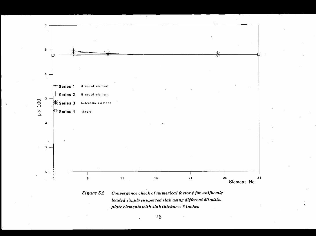
6

5

4

ISeries 1 4 noded element

Series 2 8 noded element

0 3

0 ~ Series .3 heterosis element.--<X tLJ-Series 4 theoryca.

2

o6 11 16 21 26

Element No.31

Figure 5.2 Convergerwecheck of numerical factor fl for uniformlyloaded simply supported slab using different Mindlinplate elements with slab thickness 6 irwhes

73

converges rapidly as relatively finer mesh is used. The variation of B withthe variation of slab thickness is not so significant.

5.5 Comparison of Numerical Factors a and fi for Centrally LoadedSimply Supported Square Slab and Check for Convergence.

The Theoretical value24 of numerical factor u for centrally loaded squareslab is 0.01160. No theoretical value24 of B is possible when the load isapplied as point load. Because if the load is applied as point load thetheoretical series obtained does not converge rapidly and the bendingmoments (and shearing forces) become infinitely large at the point ofapplication of the load. However if the load applied is distributed over anarea of O.la diameter the theoretical value24 of B becomes 0.298. Thetheoretical values of u and B are compared with those of thick plate solutionin Tables 5.3 and 5.4 for different element types, mesh size and platethickness. The convergence performance are examined in Figs. 5.3 and 5.4.From Table 5.3 it is observed that with all element types u value obtained forcentrally loaded slab having thickness 6 inches vary considerably from itstheoretical value. It is also observed that with the increase of elementnumber the differences also increase. In order to study thickness effect 8noded element and heterosis element are further considered and from Table5.3 it is observed that for slab having thickness 3 inches, thick plate solutiongives u values very close to the theoretical value. The difference found isonly 2.0% with a 7x7 mesh. B values obtained from thick plate solution arepresented in Table 5.4 and Fig. 5.4. It is found that with the increase ofelement number the variation of B is very significant. Compared with thetheoretical value(where load is applied over an area of O.la diameter) it isfound that when the load is applied as point load, B value obtained with a 7 x7 mesh is 54.9% greater for 8 noded element and heterosis element.However when the load is applied over an area of O.la, the differences comesdown to only 1.1% with a 5 x 5 mesh.

74,

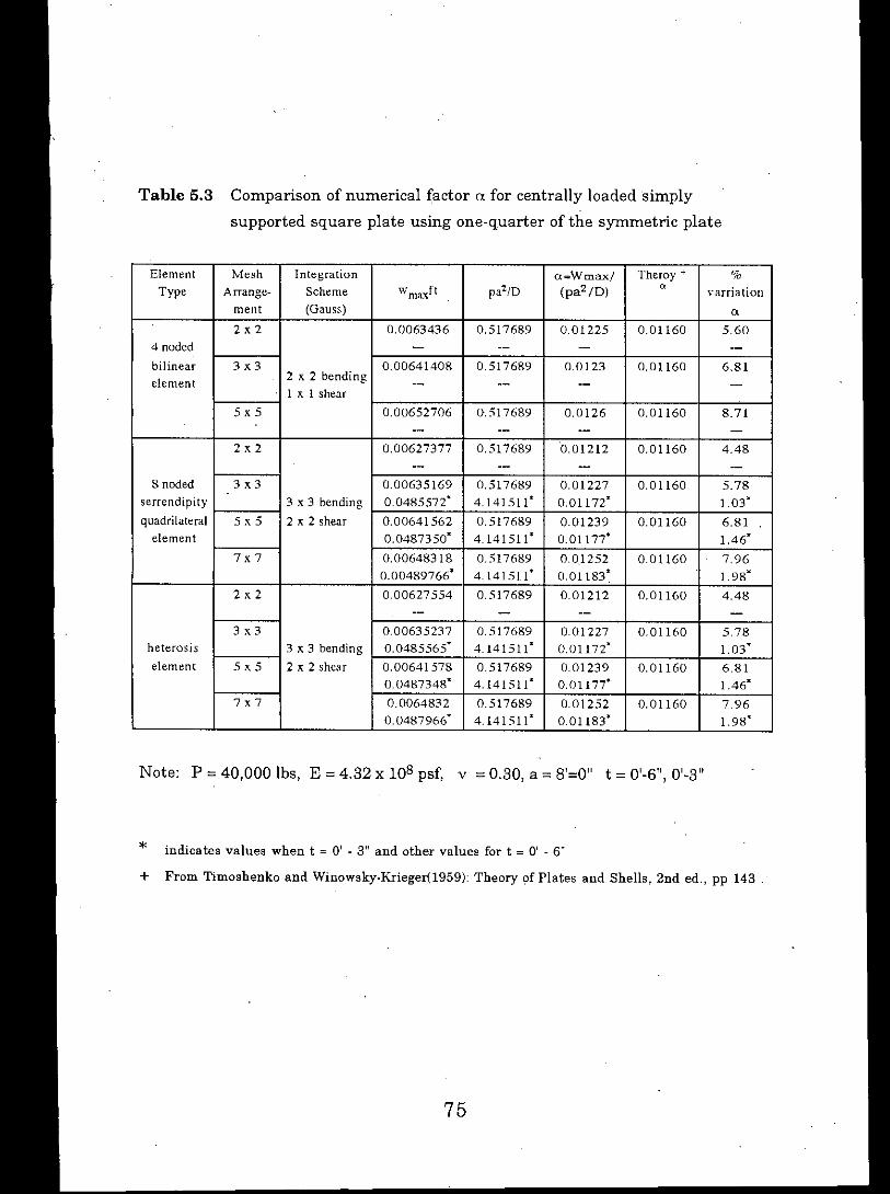
Note: P = 40,000 Ibs, E = 4.32 x 108psf, v = 0.30, a = 8'=0" t = 0'-6",0'.3"

Table 5.3 Comparison of numerical factor a for centrally loaded simplysupported square plate using one-quarter of the symmetric plate

From Timoshenko and Winowsky-Krieger(1959): Theory of Plates and Shells, 2nd ed., pp 143 .

indicates values when t =:: 0' - 3" and other values for t =:: 0' - 6"

75

+*

Element Mesh Integration a=Wmax/ Theray + %Type Arrange- Scheme Wmaxft pa2/D (pa2(D) a varriation

ment (Gauss) a2x2 0.0063436 0.517689 0.01225 0.01160 5.60

4 noded - -- - --bilinear 3x3 0.00641408 0.517689 0.0123 0.01160 6.81element 2 x 2 bending -- -- -- --

1 x 1 shear5x5 0.00652706 0.517689 0.0126 0.01160 8.71

-- -- -- --2x2 0.00627377 0.517689 0.01212 0.01160 4.48

-- -- -- --8 noded 3x3 0.00635169 0.517689 0.01227 0.01160 5.78

serrendipity 3 x 3 bending 0.0485572" 4.141511' 0.01172" 1.03*quadrilateral Sx5 2 x 2 shear 0.00641562 0.517689 0.01239 0.01160 6.81element 0.0487350" 4.141511' 0.01177' 1.46*

7x7 0.00648318 0.517689 0.0)252 0.01160 7.960.00489766" 4.141511" O.O1183~ 1.98'

2x2 0.00627554 0.517689 0.01212 0.01160 4.48-- -- -- --

3 x 3 0.00635237 0.517689 0.01227 0,01160 5.78heterosis 3 x 3 bending 0,0485565* 4.141511" 0.01172" l.03*element 5x5 2 x 2 shear 0.00641578 0.517689 0.01239 0.01160 6.81

0.0487348' 4.141511" 0.01177" 1.46*

7x7 0.0064832 0.517689 0.01252 0.01160 7.960.0487966' 4.141511" 0.01183" 1. 98*

Table 5.4 Comparison of numerical factors B for centrally loaded simplysupported square plate using one-quarter of the symmetric plate

Element Type Mesh Integration Maximum Mx B=Mmax/P Theory + % VariationArangement Scheme arMy ~*' ~

(Gauss)

2x2 6425 0.1606 0.298 u 46.11-- -- --

4 noded 3x3 2:<2 bending 7791 0.1948 0.298 ** 34.63bilinear lxl shear -- -- --element 5x5 9749 0.2437 0.298 ** 18.22

-- -- -2x2 11730 0.2933 0.298 ** 1.57

-- -- --

8 noded 3x3 13463 0.3366 0.298 ** 12.95serendipity 3x3 bending -- - --

quadrilateral 5x5 2:<2 shear 15597 0.3899 0.298 ** 30.84element 15596:1: 0.3899' 30.84'

7x7 18465 0.46163 0.298 ** 54.9118465' 0.46163* 54.91 :I:

2x2 11559 0.2890 0.298 ** 3.02-- -- --

3x3 13324 0.3331 0.298 ** II. 78heterosis 3:<.3 bending -- -- --element 5x5 2:<2 shear 15479 0.3870 0.298 ** 29.87

11786 ** 0.29465 :1::1: 1.12 **7x7 18465 0.46163 0.298 ** 54.00

-- -- --

Note: P = 40,000 lbs, E = 4.32 x 108 psf, v = 0.30, a = 8'-0", t=0'-6",0'-3"

* Indicates values with t = 0'.3". Other v~lues for t = 0' - 6"

** Indicates values when load is applied over an area of O.la dia

+ From Tlmoshenko and Winowsky-Kreiger (1959): Theory of Plates and Shells, 2nd ed., pp 150.

76

1.4

't.)I( *"1.2

0.81,Series 1 4 noded element

Series 2 8 noded element

0 ~ Series 3 heterosis element0......•0.6

X P Series 4 theory

ij

0.4

0.2

o5 9 13 17 21 25 29

Element No.Figure 5.3 Convergence check of numerical factor (l for centrally

loaded simply supported slab using different Mindlinplate elements with slab thickness 6 inches

77

5Series 1 4 noded element

Series 2 B noded element

Series 3 heterosis element

4 ~Series 4 theory

Series 5 heterosis element(load llpplied as theory)

o•....•Xco.

3

2

o

/"

6 11 16 21 26 31

Element No.Figure 5.4 Convergence check of numerical factor fJ for centrally

loaded simply supported slab using different Mindlin

plate elements with slab thickness 6 inches

78

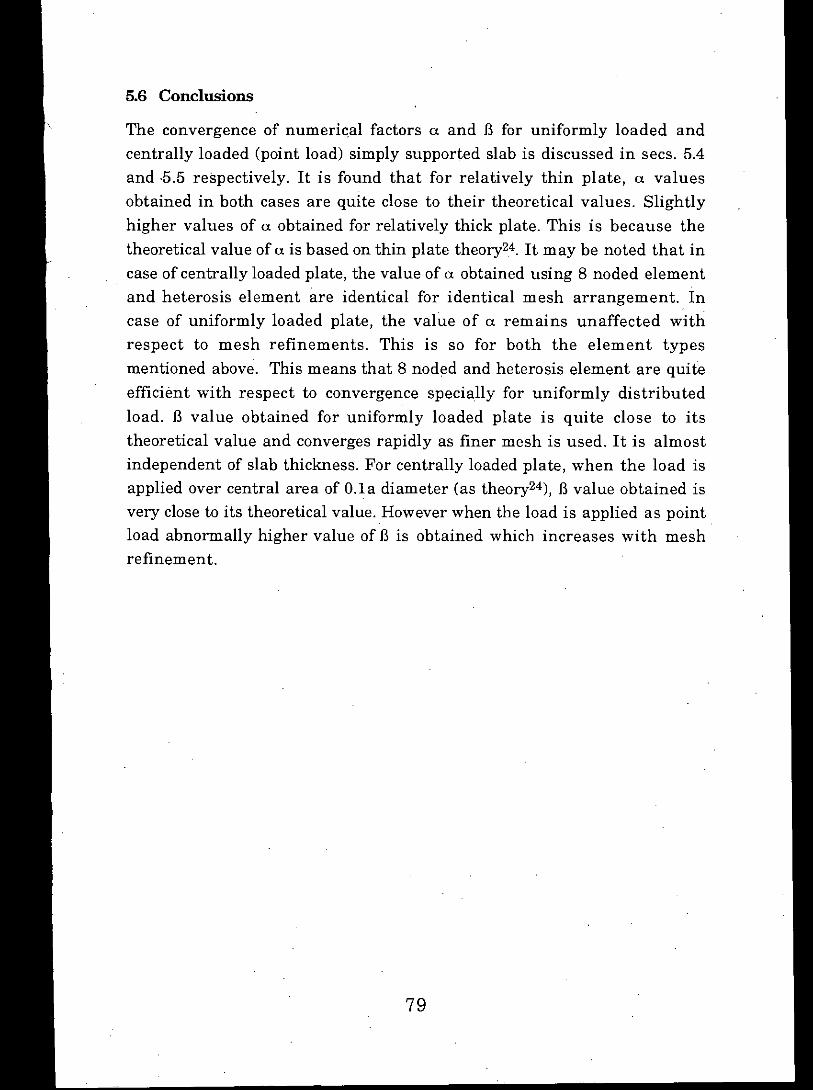
5.6 Conclusions

The convergence of numeric,al factors a and B for uniformly loaded andcentrally loaded (point load) simply supported slab is discussed in sees. 5.4and ,5.5 respectively. It is found that for relatively thin plate, a valuesobtained in both cases are quite close to their theoretical values. Slightlyhigher values of a obtained for relatively thick plate. This is because thetheoretical value of a is based on thin plate theory24. It may be noted that incase of centrally loaded plate, the value of a obtained using 8 noded elementand heterosis element are identical for identical mesh arrangement. Incase of uniformly loaded plate, the value of a remains unaffected withrespect to mesh refinements. This is so for both the element typesmentioned above. This means that 8 noded and heterosis element are quiteefficient with respect to convergence specially for uniformly distributedload. B value obtained for uniformly loaded plate is quite close to itstheoretical value and converges rapidly as finer mesh is used. It is almostindependent of slab thickness. For centrally loaded plate, when the load isapplied over central area of O.la diameter (as theory24), B value obtained isvery close to its theoretical value. However when the load is applied as pointload abnormally higher value of B is obtained which increases with meshrefinement.

79

Chapter 6

STRESS EVALUATION - SMOOTIllNG TECHNIQUE

6.1 General

Finite element analysis generally involves the minimisation of somefunctional defined in terms of piece wise functions: These functions aregenerally required to have a certain degree of inter-element continuitydepending on terms in the functional. In many finite element problems,the quantities of primary engineering interest involve the functionderivatives and in many instants, especially with lower order elements,these derivatives do not possess inter-element continuity. The analyst istherefore faced with the problem of interpreting quantities which havehistogram type distributions. Effective interpretation of these informationwill depend on the experience of the analyst with the problems in hand.Thus, such interpretations may easily. be prejudiced and may lackconsistency and rationality. In many of the automatic finite element basedsystems for linear and non-linear analysis, design and optimisationcurrently under development, it is crucial that some rational andconsistent procedures for the interpretation of discontinuous functions beadopted.

Figure 6.1 Unsmoothed stress distribution.

6.2 Smoothing Techniques .

In the displacement method, the stresses are discontinuous betweenelements because of the nature of the assumed displacement variation. A

80

5

* IV

'1 =-1

7

expression

°1' 1.866 - 0.500 0.134 -0.500 °1,-0.500 1.866 -0.500 0.134°3 °2 (6.1),

0- = 0.1340 -0.500 1.866 -0.500 0::;,,

-0.500 0.134 -0.500 1.866°7 °4

81

where OJ', 03', 05 and 0/ are the smoothed corner node values and OJ, 0"

03 and 04 are the stresses at the Gauss points as defined by in Fig. 6.2

Figure 6.2 A two dimensional parabolic isoparametric element

typical stress distribution is shown in Fig. 6.1. In analysis involvingnumerically integrated elements such as isoparametric elements, it isreported22 that the integration points are the best stress sampling points.The nodes, which are the most useful output locations for stresses, appearto be the worst sampling points. Reasons for this phenomenon are notimmediately apparent. However, it is well known that interpolationfunctions tend to behave badly near the extremities of the interpolationregion. Therefore it is reasonable to e?,pect that shape function derivatives(and hence stresses) sampleq in the interior of the elements will be moreaccurate than those sampled on the element periphery. Hinton andCampbe1l25 have shown that a technique known as 'local stress smoothing'is the natural method for sampling finite element stresses in analysesusing 2x2 Gauss integration. In this context, Local smoothing is simply abilinear extrapolation of the 2x2 Gauss point stress values. The smoothedcorner node values may be obtained from Gauss point values using the

The mid side node values may be obtained by averaging the values at nodesassociated with the side in question. Smoothed values should subsequentlybe averaged to obtain unique values at nodal points.

In the present study in addition to 4 noded element, 8 noded and heterosiselements (all based on Mindlin plate theory) are considered. The last twoelements require 2x2. Gauss integration for shear and 3x3. Gaussintegration for bending. Therefore instead of using the above method adifferent approach is considered here to compute nodal stresses. In theproposed method a linear polynomial for 2x2 Gauss integration points and aquartic polynomial for 3x3 Gauss integration points are considered toextrapolate the nodal stresses from Gauss print values. Using the co-ordinates of Gauss points the co-efficient matrices of the polynomial arecomputed through matrix inversion by computer. Then using the stressesof Gauss points the co-efficient of the polynomials and hence the nodalstresses can be computed. Once the nodal stresses are found the nodalaverage stresses can be obtained by averaging nodal stresses of differentelements meeting at a common node.

Interpolation polynomials for 2x2 Gauss point stresses is given by0= a1 + a2S + a311+ a4S11............. ( 6.2)

Therefore

OJ 1 131 111 131111 al

°1 1 132 112 132112 az

°3 = 1 133 113 133113 a3 (6.3)

°4 1 134 114 134114 a4

or

oJ 1 -0.5773502 -0.5773502 0.3333333 al

°1 1 -0.5773502 0.5773502 -0.3333333 az

°3 = 1 0.5773502 -0.5773502 -0.3333333 a3 (6.4)

°4 1 0.5773502 0.5773502 0.3333333 a4

82

knowing the values of al. a2, as and a4 stress at any point within anelement can easily be found, from Eq. 6.2 and hence the nodal average of

stresses.

(6.5)02

0.2500000.4330130.4330130.750000

0.2500000.433013-0.433013-0.750000

0.250000-0.4330130.433013-0.750000

83

0.25000-0.433013-0.4330130.750000

Interpolation polynomial for 3 x 3 Gauss point stress can be expressed as

o ~ al + a2S + ~'1 + ~s2 + aSS'l+ %'12 + a7S2'l + aSS2,l + agS2'12 (6.6)

Therefore

01 1 131 '11 1;12 131'11 '112 1312'11 131'112 1;12,112 al

02 1 132 '12 1322 132'12 '122 1322'12 132'122 1322,122 a2

oJ 1 I; '13 1332 133'13 '132 1332'13 S3'l} 1332,132 as.304 1 134 1342 134'14 '142 1342'14

~ ? 1342,142 ~'14 1;4'14-o. = 1 135 '15 1352 135'15 '152 1352'15 S5'l} 1352'152 as (6.7))

06 1 136 '16 1362 136'16 '162 I; 2 136'162 1362,162 %.6 '1607 1 137 1372 137'17 '172 1372'17

~ ? 1;72,172 a7'17 1;711r

Os 1 1;8 '18 1382 138'18 '182 1382'18 138'182 1382,182 as

09 1 139 '19 1392 139'19 '192 1392'19 1391192 1392,192 ag

"I 1.0 -0.774597 .0.774597 0.600000 0.600000 0.600000 .0.464758 -0.464758 0.36 a]

"2 1.0 -0.774597 0,000000 0.600000 0,000000 0.000000 0.000000 0.000000 0.00 a2

0:- 1.0 -0.774597 0.774597 0.600000 -0.600000 0.600000 0.464758 .0.464758 0.36 as

°4 1.0 0.000000 -0.774597 0.000000 0.000000. 0,600000 0.000000 0.000000 0,00 a4

U5 1.0 0.000000 0,000000 0.000000 0,000000 0.000000 O.oocooo 0.000000 0.00 as (68)

"6 1.0 0.000000 0.774597 0.000000 0.000000 0.600000 0.000000 0.000000 0,00 a6

"7 1.0 0.774597 -0.774597 0,600000 -0.600000 0.600000 -0.464758 0.464758 0.36 a7

"8 1.0 0.774597 0,000000 0.600000 0.000000 0.000.000 0.000000 0.000000 0,00 as

°9 1.0 0.774597 0.774597 0.600000 0.600000 0.600000 0.464758 0,464758 0,36 ag

Taking inversion of the matrix we get,

Knowing the values of aI, a2 a9 we can easily find the stresses of any

point within an element usmg Eq. 6.6 and hence the nodal average ofstresses.

0,694444 -'.388889 0.694144 .1.388889 27m78 .1.368889 0,694444 -'368889 0,694444

(6.9)

0'".'

°70.537914

0.410067

00

00

00

00

0.833333 0,0

0.0

0,545<197 0,0

0.0

0,537914 -'075829 0537914

-0416667 00

0.0

0.0

00

-1.075829 -0537914 00

0.0

0.0

0.0

0.645497 0.0

00

".6€6667 0,0

00

1.0

00

00

0.0

-0645497 0.0

0833333 -1.666667833333 0,0

00

-0.416667 0,0

0.537914 1.075829 0.0

0.0

0.0

0.0

0.833333 00

00

00

00

-0.537914 1.075S29 -0.537914 00

84

0.0

0,41E667 0.0

0.0

-0 537914 0,0

0.0

0.0

000000o -0.645497 0.00lXl00 0,0000

ag

as

as

Taking inversion of the matrix we get

85

-II"

D

(b) 5 x 5 meshA

c21 22 23 24 25

16 17 18 . 19 20

11 12 13 14 15 4'.

@ (j) @ @ @

CD @ @ @) @

4'-0"

D

B

q = 900 psf, a = 8'-0", t = 0'-6", E = 4.32 x 108 psI.v= 0.30)

(a) 2 x 2 mesh

(Data:

from their Gauss point values. The nodal moments (Mx) computed with themoments of integration points using quartic polynomial together with thetechnical of nodal average stress are presented in Fig. B.l of appendix B.The comparison of these moments with theoretical values along the centreline ofthe slab is given in Fig. 6.4. The theoretical maximum moment (MxJat point D (Fig. 6.3) is 2760 lb - ft/ft. Using the smoothing technique themoment (Mx) obtained at point D with a 2x2 mesh is 2830 Ib- ftlft which is

2.50/( greater than the theoretical value. With a 5x5 mesh the moment (Mxi

Figure 6.3 Mesh layout for a quarter of uniformly loaded simplysupported square slab.

A

c

To study the performance of the proposed smoothing technique discussed insec. 6.2, a simply supported square slab under distributed loading (a quartet.slab shown in Fig. 6.3) is firstly considered. In descritzation of the slahheterosis element is used which requires 3x3 Gauss integration forbending. Thus quartic polynomial is required to compute nodal moment

6.3 Checking the Perfonnance of Smoothing Technique

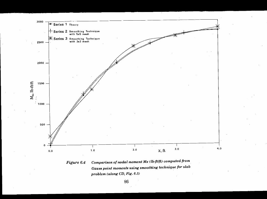
2000

4.03.0x, ft'2.01.0

Series 1 Theory

0.0

o

500

Series 2 Smoothing Techniquewith 5x5 mesh

Series 3 Smoothing Technique2500 ---.J with 3x3 mesh

3000

<t: 1500a:;,..a•...•

i1000

Figure 6.4 Comparison of nodal moment Mx (lb-ft/ft) computed fromGauss point moments using smoothing technique for slab

problem (along CD, Fig. 6.3)

86

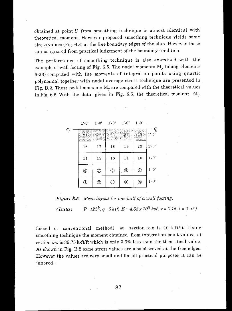
87

p= 125k, q= 5 ksf, E = 4.68 x UP ksf, v= 0.15, t = 2'.0")(Data:

Figure 6.5 Mesh layout for one.half of a wall footing.

(based on conventional method) at section x-x is 40-k-ft/ft. Usingsmoothing technique'the moment obtained from integration point values, atsection x-x is 39.75 k-ftlft which is only 0.6% less than the theoretical value.As shown in Fig. B.2 some stress values are also observed at the free edges.However the values are very small and for all practical purposes it can beignored ..

obtained at point D from smoothing technique is almost identical withtheoretical moment. However proposed smoothing technique yields somestress values (Fig. 6.3) at the free boundary edges of the slab. However thesecan be ignored from practical judgement of the boundary condition.

The performance of smoothing technique is also examined with theexample of wall footing of Fig. 6.5. The nodal moments My (along elements3-23) computed with the moments of integration points using quarticpolynomial together with nodal average stress technique are presented in ,Fig. B.2. These nodal moments My are compared with the theoretical valuesin Fig. 6.6. With the data given in Fig. 6.5, the theoretical moment My

~~

'-":i

50

40

30

20

10

o

..10

Series 1 Theory

Series 2 Smoothing Technique

0.0 1.0 2.0

y, ft3.0 4.0

Figure 6.6 Comparison of nodal moment My (k.ftlft) computed from

Gauss point moments using smoothing technique forwall footing (Fig. 6.5)

88

Heterosis element used in the analysis of wall footing of Fig. 6.5 requires 2x2Gauss integration for shear. Thus as discussed in sec. 6.2 lineal'polynomial Eq. (6.1) is needed to compute nodal shear from their Gausspoint shears. Using linear polynomial together with the technique of nodalaverage stress the nodal shear along elements 3-23 of Fig. 6.5 are shown inFig. B.3. The comparison of these nodal shear with the theoretical values isgiven in Fig. 6.7. The theoretical shear along section x-x of Fig. 6.5 is 20 klft.Using smoothing technique this shear is obtained about 20.4 klft which isonly 1.8% greater than the theoretical values. As shown in Fig. B.3 someshear values are also observed at the free edges. However the values areshall and can be ignored.

89

<!>

~

&

25

20

15

10

5

o

Series 1 Theory

Series 2 Smoothing Technique

0.0 1.0 2.0Y,ft

3.0 4.0

Figure 6.7 Comparison of nodal shear Qy (k 1ft) computed (rom Gauss

point shear using smoothing technique for wall footing

(Fig. 6.5)

90

6.4 Conclusions

In computing nodal stresses from the stresses of integration points theperformance of linear and quartic polynomial together with the nodalaverage stress is studied in this chapter. It is found that nodal stressescomputed with this technique shows excellent agreement with thetheoretical stresses. However with this technique some stresses areobserved at the free boundary nodes. This is probably because boundaryconditions are not incorporated in this technique. But when relatively finermesh is used, the discrepancy arises at the boundary is quite small and itcan be ignored for all practical purposes.

91

Chapter 7

APPROPRIATE ORDER OF QUADRATUREFOR MINDLIN PLATE ELEMENTS

7.1 General

The three different plate bending elements considered in the present studyare based on the theory of Mindlin plates. The main problem with theseelements is that they can suffer from 'shear locking' as the thickness tolength ratio becomes small. Various methods can be used to alleviate thisproblem, the most common of which is reduced integration16. Thetechnique of reduced integration ensures the singularity of ks and a propersolution is obtained over the 'thin plate' range. However reduced integrationmay lead to spurious zero energy modes or 'mechanism'and theperformance of the elements can deteriorate when they are distorted. Asdiscussed in sec. 3.5.1 the 4 noded and 8 noded elements have two and oneadditional zero energy modes respectively. In conventional plate bendingproblems (simply supported, clamped) this unacceptable situation isavoided by the presence of precious boundary restraints which suppress theactivation of spurious zero-energy modes. In foundation where sufficientrestraints are absent, these modes may show up giving spurious results. Infollowing sections, the correct order of quadrature both slab and footing

problems.

7.2 Appropriate Order of Quadrature for Mindlin Plate Elements inSlab Analysis

One-quarter of a simply supported slab shown in Fig. 7.1 is considered tostudy appropriate order of quadrature for different Mindlin plate elementsin analysis of conventional plate bending problem. With slab thickness :3inches, the theoretical maximum moment (Mx & My) and verticaldisplacements obtained are 1.694 k-ftjft and 0.02605 ft respectively. Thetheoretical maximum vertical displacement becomes 0.003256 ft whenthickness of the slab is used 6 inches. Using different mesh arrangements'and slab thickness the vertical displacements and moments values obtainedfor different Gauss quadrature are compared with those of theoretical to

identify the correct order.

92

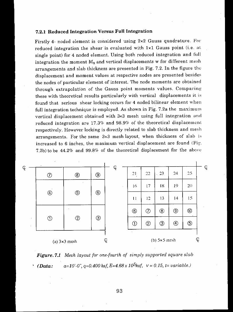
Figure.7.1 Mesh layout for one-fourth of simply supported square slab

7.2.1 Reduced Integration Versus Full Integration

Firstly 4- noded element is considered using 2x2 Gauss quadrature. Forreduced integration the shear is evaluated with 1x1 Gauss point (i.e. atsingle point) for 4 noded element. Using both reduced integration and fullintegration the moment Mxand vertical displacements w for different mesharrangements and slab thickness are presented in Fig. 7.2. In the figure thedisplacement and moment values at respective nodes are presented besidesthe nodes of particular element of interest. The node moments are obtainedthrough extrapolation of the Gauss point moments values. Compal.ingthese with theoretical results particularly with vertical displacements it isfound that serious shear locking occurs for 4 noded bilinear element whenfull integration technique is employed. As shown in Fig. 7.2a the maximumvertical displacement obtained with 3x3 mesh using full integration andreduced integration are 17.3% and 98.9% of the theoretical displacementrespectively. However locking is directly related to slab thickness and mesharrangements. For the same 3x3 mesh layout, when thickness of slab isincreased to 6 inches, the maximum vertical displacement are found (Fig.7.2b) to be 44.2% and 99.8% of the theoretical displacement for the above

(b) 5x5mesh

21 ')') .23 24 25--

16 17 18 19 2()

11 12 13 14 15

@ (J) @ @ @

CD @ CID @) @

93

a=10'-0", q=0.400 ksf, E=4.68 x l05ksf, v = 0.15, t= variable.)

(a) 3x3 mesh

(Data:

~

(J) @ @

@) @ @

CD @ CID

cases respectively. Using 5x5 mesh layout, the maxlmuIIl; verticaldisplacement obtained with reduced integration are 100.0% and 100.8'lr ofthe theoretical displacement for slab thickness 3 inches and 6 inchesrespectively. With full integration they are found 26.4% and 61.2'lc of thetheoretical displacement respectively. Therefore larger locking occurs forcases when thickness to length ratio of the element becomes smaller.

Using 8 'noded element and heterosis element the moments Mx and verticaldisplacement w for different mesh arrangements and slab thickness arecompared for the same problem in Figs. 7.3 and 7.4. It may be mentionedthat for these elements basically 3x3 Gauss quadrature is employed with2x2 integration for evaluation of shear. It is observed that locking is lesssignificant for 8 noded element and heterosis element. As shown in Figs.7.3a and 7Aa the maximum vertical displacement obtained for fullintegration and reduced integration with 3x3 mesh layout are 99.2'lr and100.0% of the theoretical displacement respectively for both elements.However when either thickness of the slab is increased or mesh layout isrefined full integration and reduced integration yield almost identicaldisplacement for both elements and are identical with theoreticaldisplacement as well. Therefore in relatively thick plate with fine meshshear locking is negligible for 8 noded element and heterosis element.

From Fig. 7.2 it is to be noted that due to shear locking, in addition todisplacement, significant moments reduction occurs for 4 noded element.For 8 noded element and heterosis element shear locking is found negligibleand moments obtained for both elements using reduced integration and fullintegration are almost identical (Figs. 7.3 and 7.4).

7.2.2 2x2 Gauss Integration

A separate analysis has been carried out for 8 noded element and heterosisusing 2x2 Gauss integration scheme for bo~h shear and moment. Bendingmoment and deflection results obtained are presented in Fig. 7.5. It may benoted that a 2 x 2 integration for bending and shear yields displacementsidentical to that of reduced integration of in Fig. 7.3d. However themaximum moment obtained is about 0.8% greater in case of 2x2 integrationscheme. In order to examine the performance of 2 x 2 gauss integration(both for bending and shear) the vertical displacements along the centre line

94

95

Figure7.2 Comparison of moments Mx (k-ftlftj and displacements w (ff)in simply supported slab using different mesh arrangementsand slab thickness for reduced integration and full integrationwith 4 noded element.

0.003133 RI)0.001853 FIr

0.003282 RI)0.001943 FI J'"

0.003250 RIl W0.001438 FI r

1.7552 RI1.2004 FI

M"f 1.6942 RIL 1.0131 FI

Theoreticalwmax=0.0032566ftMax. Mx=MaxMy= 1.6949.k-ft/ft

(d) Element 25,5 x 5 mesh, t = 0'-6"

0.003095 RI]w__-------<11 0.001332 FI I(b) Element 9,3 x 3 mesh, t = 0'-6"

M,,[RI 1.6494FIO.9808

M,,[ RI 1.6462FIO.8318

0.02604 RI}0.006884 FI W

M,,[1.6942 RI0.4565FI

Theoretical 0.02577 RI}Wwmax=0.026051ft 0.004495 FIMax.Mx=Max My= 1.6949 k-ftlft

(c) Element 25, 5 x 5 mesh, t = 0'-3"

M,,[ 1.6494 RI0.4406FI

(a) Element

M,,[RI 1.6458 M,,[ 1.7545 RIFI 0.3994 0.5151 FI

0.02455 RI}W.__------ ...•. 004133 FI

9, 3 x 3 mesh, t = 0'-3"

0.024866 RI}_--------- 0.006563 FI W

of the (simply supported) slab are plotted in Fig. 7.6. It is found that thedisplacement profiles represent smooth curves both for 8 noded andheterosis element, no hour-glass (oscillating behaviour) mode is obselved.

This indicates that no spurious mechanism occurs.

Ji'igure7.3 Comparison of moments Mx(k.ftlft) and displacements w(ft) insimply supported slab using different mesh arrangements andslab thickness for reduced integration and full integration with8 noded elements.

96

0.003293 RI)0.003291FI II\'

0.003294 RI)0.003272FI IW

M,[ 1.7008 RI1.6981 FI

M'f 1.6981 RIL 1.7039FI

(b) Element 9,3 x 3 mesh, t = 0'.1)"

0003144 RI 10.003142 FI II\'

~------ ..(d) Element 25,5 x 5 mesh, t = 0'.6"

0.003146 RII0.003123FI IW..---------

M,[RI1.6600FI1.6567

M,[RI 1.6747FI1.6447

0.02445RI}0.02466 FI W

0.02613 RI}0.02583FI w

0.02496RI}0.02492 FI W

0.02614 RI.}0.02610FI W

M,[1.7009 RI1.6995 FI

M,[1.6929 RI1.6908 FI

(a) Element 9, 3x3 mesh, t = 0'.3".

(c) Element 25, 5x5 mesh, t = 0'.3"

M,[ RI 1.6601FI1.6527

M,[ RI 1.6720FI1.6237

97

Figure 7.4 Comparison of moments' Mx and displacements w in simp(vsupported slab using different mesh arrangement for reducedintegration and full integration with heterois elements, t = 0'-8 ",

0.02614 RIj0.02609 FI IW

M'f 1.7007 RIL 1.6943FI

25

(b) Element 25, 5 x 5 mesh

(b) heterosis element, 5 x 5 mesh

0.02496 RI I0.02491 FI r

W

~------'

M,[RI 1.6599FI1.6519

0.02614 RI}0.02585FI w

MX[1.6865 RI1.7146FI

(a) Element 9, 3x3 mesh

Figure7.5 Moment Mx (k-ftlft) and displacement w(ft) in simplysupported slab with 8 noded element and heterosis elementusing 2 x 2 Gauss integration both for bending and shear, t = 6"

(a) 8 noded element, 5 x 5 mesh

Mx=1.6727 1.6928 1.7139 Mx = 1.6728 1.6928 1.7139.

0.003293=w 0.003293=w

@0.003256=w @

0.003256=w

0.003144=w 0.003145=w

0.02496 RI}0.02466 FI W....--------..

@

M,[ RI 1.6831FI1.6262

m I

~s:

1.2

0.8

0.6

0.4

Series 1 With 8 noded element

Series 2 With heterosis element

0.2

o0.0 0.1 0.2 0.3

x/L0.4 0.5

Figure 7.6 Vertical displacement along the certre line ofsimplysupported slab (Fig. 7.1b)with 8 noded- and heterosiselement for 2x2Gauss integration for both bendingand shear

98

7.3 Appropriate Order of Quadrature of Mindlin Plate Elements inFoundation Analysis.

To examine correct order of quadrature for different Mindlin plate elementsin analysis of foundation, three different types of footings i.e. wall footing,square footing and eccentric footing are considered. Using different meshlayout and slab thickness the vertical displacements and moments fordifferent order of Gauss quadrature are studied with the element typesdiscussed in sec. 3.5.1. Since heterosis element has the correct rank,vertical displacements and moments of the above foundation problemsusing heterosis element are firstly studied. The displacements andmoments for other elements are then compared with those of hete)'osis

elements.

7.3.1 Reduced Integration Versus Full Integration in Wall Footing

To examine the appropriate order of quadrature for different Mindlin plateelements in analysis of foundation, wall footing shown in Fig. 7.7 isconsidered first. Load applied is uniformly distributed over elements 7,8 and9 in Figs. 7.7a and 7.7b and over elements 21,22,23,24 and 25 in Fig. 7.7c,Magnitude of the load and dimensions of the footing are adjusted in such away that an uniformly distributed upward pressure of magnitude of 5 ksfdevelops under rigid plate condition.

If the loaded nodes are considered fixed, the theoretical moment My atsection xx would be 40 k.ft/ft. Firstly the analysis is carried out withheterosis element. Moment My and displacement w obtained using reducedintegration and full integration for various mesh arrangements and footing,thicknesses are shown in Fig. 7.8. From Fig. 7.8a it is found that when thethickness of the footing is comparatively small (t=1'-0") full integrationtechnique leads to shear locking. This is reflected from the fact that whenfull. integration technique is employed the vertical displacements becomemore uniform all over and the maximum restrained moment My is 8.57rless than the value obtained using reduced integration. When the footingthickness is increased (t=2'-0") reduced and full integration give almostidentical displacements, but maximum My is observed to be 2.57r lowe)'tha'n the reduced integration value. From Fig. 7.8b where different element

99

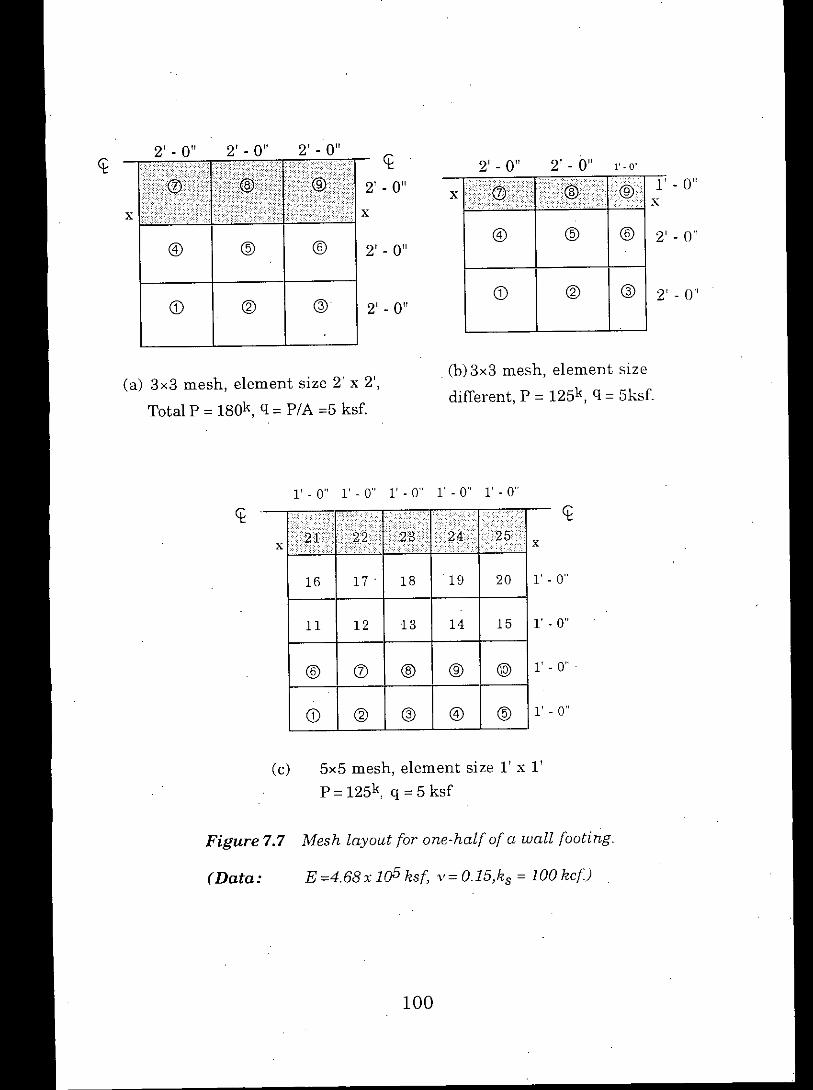
. (b)3x3 mesh, element size

different, P = 125k, q = 5ksf.

100

E =4.68 x 105 ksf, v= 0.15,ks = 100 kef)(Data:

l' . 0" l' - 0" l' - 0" l' - 0" l' - 0"

Ci: Ci:

X X

16 17 . 18 19 20 l' - 0"

11 12 13 14 15 l' . 0"

@ ([) @ @ @) l' - 0" .

CD @ @ @ @ l' - 0"

(el 5x5 mesh, element size l' x l'

P = 125k, q = 5 ksf

Figure 7.7 Mesh layout for one-half of a wall footing.

Ci: 2' - 0" 2' - 0" 1'.0"

2' - 0" xl' - ()"x

x

@ @ @@ @ @ 21

- on2' - 0"

CD @ @CD @ @ 21

- 0'12' - 0"

(al 3x3 mesh, element size 2' x 2',

Total P = 180k, q = PIA =5 ksf.

101

7.7c

My MyW W W

0.05025 RIO.05143 I 005035 m0.05025 RIO,05144 0.05025 FI

0.05025 RI 0.05142 0.0 " 0.050340.05025 FI 0.05138 2:; 0.0503-'\

0.05023 0.05137 39.390 39757 0,0[,022

0.05022 0.05138 38.803 39.606 0.05022

0.05012 0.05120 30.484 0 31.012 0.0501::i

0.05012 0.05121 30.485 31.011 0,05017

18

0,04995 0.05085 21.585 22.283 0,05011

0.04995 0.05085 21.676 22.302 D.OSOll

0.04977 0.05037 15.408 o 15,933 0.05004

0.04977 0.05037 15.411 15.953 0.05003

MyMy

O.U 0

@

~: 38.316 39.014 RII 35.074 38.030 FI

23.334 0 23.98923.348 23.986

@

8.554 9.0679.651 9.390

3.915 o 4.0673:901 4.068

C?J

0.04973 0.048530.04973 0.04856

0.05008 0.050910.05008 0.05091

0.04991 0.049830.04991 0.04985

0.05018 0.051430.05018 0.05139

0.05023 RI 0,051490.05022 PI 0.05143

w W0.05024 RIO.051490.05024 FI 0.05149

MyMy

0.0 0

@

~!38.098 38.991 RIFI 34.880 38.009 PI

23.235 23.96223.247 o 23.950

@

8.522 9.0089.611 9.335

3.881 o 4.0573.870 . 4.061

<.?J

0.048290.04832

0,050650.05065

0.049580.04960

0.051260.05123

.0.051170.05114

0.04691 0.04954 0.04715 0.04959 @0,04696 0.04954 0,04718 0.04959 1- --'

(t=I'.O") (t=2'.O")(t=I'.O") (t=2'.1I") (t=I'.O") It=2'.U',

(a) 3x3 mesh of Fig. 7.7a (h) 3x3 mesh of Fig. 7,7h (c) SxS mesh or Fi~

W.

RI 0.05128FI 0.05125

. Figure 7.8 Moments My (k-ftlft) and vertical displacement w (ft) in wallfooting with different mesh layout and footing thickness forreduced and full integration.

sizes are mixed a similar observation is made. As shown in Fig. 7.8c whenthe mesh is refined full integration and reduced integration give identicalvertical displacements for all footing thickness. However for full integrationmaximum My is reduced by 1.4% when thickness used is 1 ft and O.4'1rwhen thickness is 2 ft. Therefore, in relatively thick plate locking effect isfound to be negligible when the mesh is refined. It should be noted thatstiffness matrix derived from heterosis element using reduced integrationhas correct rank. On the other hand stiffness matrix derived from 8 nodedor 4 noded element (using reduced integration) is rank deficient. Therefore,as discussed in sec 7.1 spurious results may be obtained for these elements.But comparing the results of Fig. 7.8c, with that of Fig. 7.9 it is observed that8 noded element gives results almost identical to that of heterosis element.Because of assumed linear displacement function for 4 noded element, the

Figure 7.9 Comparison of moments My (k-ft 1ft) and vertical displacementsw (ft) in wall footing using 8 noded - and 4 noded elements forreduced integration and full integration with t = 2' - 0",

My

0.049600.04962

w

0.049770.04979

0.049960.04996

0.050120.05011

x0.050220.05021

0.05025RI0.05025FI

23

RI31.31FI28.75

18

23.6621.74

13

11.2010.27

@

3.753.43

@

x

(b) 4 noded element

0.049680.04968

0.049950.04995

0.050040.05003

0.049590.04959

0.049860.04986

0.049770.04977

0.050120.05011

0.050180.05017

102

x0.050220.05022

0.050240.05024

0.05025RI0.05025FI

w

23

RI 39.811FI39.658

18

22.25622.224

13

9.7219.743

@

2.2562.276

@

x

(a) 8 noded element

7.3.2 Reduced Integration Versus Full Integration in Square Footing

l' - 0"

l' - ()"

l'-{Y'

1.r - O"

15

20

14

19

@)

13

18

@

12

17

11

16

11 _ Ol! l' _ 011 11 _ 0" l' - 0" 1.' - ()'!<i:

21,.,,., 23 24 [' - 0"

103

E=4.68xl05ksf, v=O.15, t=2'-O",PI4=125k, q =PIA = 5 !lsf

Shaded area indicates the loaded zone,)(Data:

Figure7.10 Mesh layout ofa quarter ofa square footing.

A square footing as shown in Fig. 7.10 is considered next. Using differentMindlin plate elements together with reduced integration and fullintegration the moment My and vertical displacement w at some of the

mements approach a constant values with each element but has differentvalues in different elements. Thus, while the displacements obtained using4 noded element are close to those of 8 noded element and heterosis element,the extrapolated nodal moment (and shear) of 4 noded element differsignficantly from respective quantities obtained using the other twoelements. However, comparing the vertical displacements along withmaximum restrained moment My it is found that shear locking do occur f()l'.4 noded element when full integration technique is employed.

nodes are presented in Fig. 7.11. Comparing the vertical displacements ofFigs. 7.11a and 7.11b it is found that reduced integration and full integrationyield identical displacements for both 8 noded and heterosis element..However full integration technique reduces the maximum My by about O.57rfor both elements. Like simply supported slab and wall footing the momentsand displacements obtained for square footing with 8 noded element anifound very close to that of heterosis element. But the maximum My obtained(Fig. 7.11c) for 4 noded element differ considerably compared to heterosis or8 nodded element. Though the displacements obtained are comparable tothose of other types of elements, some locking is observed for this elementwith full integration technique.

Figure7.11 Moments My (k-ftlft) and displacement w (ft) in square footing

for reduced integration and full integration using differentMindlin plate elements.

0.049980.04997

0.050220.05020

0,049750.04975

0.0504S0.05045

x0.050'700,05066

W

0.05081 RIO.OS076FI

M

(c) 4 noded element

.'v

25

RI5489F150.63

:n

39.653687

15

15.521397

@

9.417.39

@

w0.05083PJ0.05083FI

0.050810.05081x x0.050740.05074

0.05064 .0.05063

0.050510.05051

0.050380.05038

0.050250.05024

0.050110.05011

0.0499d0.049d8

0.049870.04986

0.04975004975

My

(b) 8 noded element

25

RI 78.51F178.14

:n30893101

15

10.821085

@

193195

@

x

0.050380.05038

0.049750.04975

0.050250.05024

0.050110.05011

0.049990.049d8

0.049870.04986

0.050520.05051

0.050640.05063

0.050810.05080x0.050740.05073

104

W0.05083RI0.05082FI

M'v25

1<180.78FI80AO

:n

29.8729.98

15

10.8710.91

@

1S91.92

@

(a) Heterosis element

x

105

7.3.3 2x2 Gauss Integration in Square Footing

0.04975

0.04986

0.04999

0.05011

0.05025

0.05038

0.05052

0.05069

x0.05074

0.05081

M W0.05083

"v

25

83.627

20

29.970

15

10.82

@

1912

@

(b)Heterosis element

0.04975~o

31 6 0.05051 .

15 0.05038

10. 77 0.05025

@ 0.05011

1. 28 0.04999

@ 0.04987

Figure7.12 Moments My (k-ftlft) and displacement w (ft) in square footingusing 2 x 2 Gauss Integration both for bending and shear for8 noded element and heterosis element.

(a) 8 noded element

M W

0.05083

25 0.05081

.x x x79. 6 0.05074

20 0.05064

A 2 x 2 Gauss integration both for bending and shear is performed forheterosis and 8 noded element (Fig. 7.12) and found that the (like simplysupported slab) 2 x 2 integration and reduced integration give identicalvertical displacements. However, comparing with the moments of reducedintegration of Fig. 7.11 it is observed that a 2 x 2 gauss integration(for bothbending and shear) increases the maximum restrained moment My by3.5%for heterosis element and 1.5%for 8 noded element.

7.3.4 Reduced Integration Versus Full Integration in Eccentric Footing

An eccentric footing shown in Fig. 7.13 is finally considered next. From Fig.7.13 it is observed that the vertical displacements obtained with 8 nodedelement is very close to that of heterosis element. It is also observed thatvertical displacement obtained with 8 noded element using reducedintegration and full integration are almost identical. However comparingdisplacements from the figure some locking is observed with heterosiselement when full integration technique is employed.

1".0" 1".4.5" 1".3" 1".4.5" 1".0"8 noded heterosis

-0.011 RI -0008 RI 0.085 RI 0.085 RI 0172RI 0170 RI-0.011 FI -0007 FI 0.085 FI 0.085 FI 0.172 FI 0.168 FI

-0084 RI -0080 RI 0003 RI 0.005 RI 0.099 RI 0.099 RI-0.084 FI -0.077 FI 0.003 FI 0006 FI 0099 FI 0.098 FI

8 noded heterosis

-0.098 RI -0093 RI -00005 RI 0.085 RI 0085 In-0098 FI -0090 FI 0.0021 FI 0085 FI 0085 FI

8 noded

-0181 RI -0.174RI -0.093 RI 0.003 RI 0.005 RI-0.180 FI -0090 FI -0093 FI 0.003 FI 0006 FI

@ !J) 8 noded heterosis @

-0.194 RI -0.187 RI -0098 RI -0094 RI -0011 RI -0009 RI-0194 -0 182 FI -0.098 FI -0090 FI -0.011 FI -0007 FI

8 noded heterosis @ @ @ @

-0.268 RI -0259 RI -0.181 RI -0.174 -0.084 RI -0081 RI.0.268 FI -0.252 FI -0 181 FI -0 169 -0084 FI -0077 FI

Figure 7.13 Vertical displacement of eccentric footing using reducedintegration and full int~gration for 8 noded element andheterosis element. '-' sign indicates footing soil separation.

(Data: p= 60k, Mx = My = 120 k-ft, E = 4.68 x lOS ksf,v= 0.15, ks= 100kcf)

106

7.4 Conclusions

It is known that the best order of quadrature is usually decided afternumerical testing. Thus the order of integration of different Mindlin plateelements is examined in this chapter before going for detail study onfoundation. It is found that for Mindlin plate elements reduced integrationis the best order. As discussed in see. 3.5.1 stiffness matrix derived frombilinear element with reduced integration (2 x 2 bending 1 x 1 shear) is rankdeficient and this may lead to spurious results for foundation type problemwhere sufficient boundary restraints are absent. But comparing thedisplacements of other elements (sec. 7.3) it is found that no spm'iousresults occur for this clement for the type of footings considered. Moreoverwhen full integration (2 x 2 integration for both bending and shear) isemployed with this element, significant shear locking occurs for slab typeproblem. Locking is also observed for foundation type problem, but to alesser degree.

Stiffness matrix derived from 8 noded element is also rank deficient but.heterosis element has the correct rank. However comparing the resultsfrom sees. 7.2 and 7.3 it is found that the results obtained for these two typesof element are almost identical. Therefore, like heterosis element, 8 nodedelement can also be considered as good performing element. When fullintegration technique (3 x 3 integration for both bending and shear) isapplied it is found that locking effect is negligible for 8 noded 01' heterosiselement compared to bilinear element. For these element it is found thatreduced integration (3 x 3 bending, 2 x 2 shear) and full integration yieldalmost identical results, particularly in relatively thick plate with finemesh. Since the expense of numerical integration is proportional to theintegration point times the square of the number of element d.o.f, a loworder rule is always desirable to reduce the computation cost. Thus for Snoded or heterosis element reduced integration can be considered the mostappropriate order. As discussed in sees. 7.2 and 7.3 it found that for theseelement even a 2 x 2 integration for both bending and shear can be usedwithout causing numerical disaster.

107

Chapter 8

THICK PLATE ANALYSIS OF FOOTINGSAND MAT FOUNDATION

8.1 General

One main objective of present study is to analyse different types of footingswith Mindlin plate elements. The performance of different Mindlin plateelements has already been discussed in chapters 5 and 7. Here 8 nodedelement and heterosis element together with reduced integration techniqueare used. Types of foundations considered in the study includes spreadfooting, eccentric footing, pile foundation and mat foundation. Thenumerical examples for most of the above problems are taken from Ref. 4,for the purpose of comparison. In the study emphasis are given to thefollowings :

1. Ma,ximum moments in wall footing and column footing and theircomparison with moments obtained using ACI method.

2. Modelling the distribution of column moments to element nodesrepresenting column area.

3. Eccentric footing and soil separation.

4. Effect of cap rigidity on pile loads and pile moments.,

5. The moments of mat foundation and their comparison with momentsobtained using different approximate methods.

6. The effect of self weight on displacements and moments of foundation.

8.2 Comparison of Maximum Moments of Wall Footing and ColumnFooting.

Wall footing and column footing shown in Fi~. 8.1 are considered tocompute the maximum moment in the footings and compare them with themoments obtained using ACI method. The geometry and loading of thefooting are made comparable for ease of comparison. For footingssupporting masonry wall or column free rotation of the loaded nodes areallowed. For footing supporting RC wall fixed rotation of the loaded area areconsidered, while for column footing (supporting RC column) three differenttypes of column fixity models are considered.

108

109

x

Plan

500 K

.1,

t 2'-OJ~-4'-O-" -tElevation

(b) Column footing

e- - - - - - - - - - - - - - -I I

2'-0"

x

250 K

.I.

t 2'-OJ~4-'-O-" ~tElevation

- - - - - - --

Plan

(a) Wall footing

. I

4'-0"

2,-0,IX1

X

Figure 8.1 Plan and Elevation of a) wall footing and b) columnfooting used for numerical analysis.

t

FigureB.2 Mesh layout for one-half of wall footing shown in Fig. 8.1 a

110

E = 4.6Bx 105 ksf, v = 0.15, t = 2'-0", ks= 100 kef,P /4 = 125h)(Data:

Allowing rotation of the loaded nodes, the moment My in wall footing areshown in Fig. 8.4. The ACI theoretical maximum moment under thiscondition is 50.63 k-ft/ft which is computed considering net soil pressure atcritical section PQ i.e. at a distance w/4from wall face, where w is the widthof the wall. The average maximum moment obtained from thick platesolution is 51.52 k-ft/ft which is very close to the theoretical value, thevariation is only 1.8%. However the numerical maximum moment occursat section xl-xl i.e. about the centre line of the footing, while the theoreticalmaximum value is based on assumed critical section located at distance ofw/4 within the wall.

8.2.1Wall Footing

The mesh layout of wall footing of Fig. 8.1 is shown in Fig. 8.2. 8 nodedquadratic element is used to discretize the footing. Considering the loadednodes to be fixed against"rotation, the moments Myare presented in Fig. 8.3.The ACI theoretical moment at section x-x with this fixity condition is 40 k-ft/ft. Comparing the numerical results (Fig. 8.3b) with the theoretical valueit is found that the present finite element formulation shows excellentcorrelation. From Fig. 8.3b, it is observed that with a 5 x 5 mesh the moment.variation at section x-x near element 23 is only 0.5% and at the edges isabout 0.1%. Even with a coarse mesh of 3 x 3 the results are in quite goodagreement with theoretical value.

Figure8.3 Moment My (k-ftlft) in wall footing for different mesh layout.* indicates nearest Gauss point values.

40.04

x

"40.112

45.66 Q

S()5-+

"I

(b)

40.61

0.0 0.0 00 0.0

Z3 24 25

39.80 39.81 39.80 39.39 39.04 39.88

* * "'37.82 37.48 3:.77

@ @ @

x

40.52 40.64

::;16::; ':;1 7R

4052

x

39.37

4048

(a)

4052

.- - - - .- - - - - -5038 5033 5038

* * :I:

24 25

* * * 4654 46.684{).52 4{).49 46.52

*" * *42.67 4364 42.67

111

,,1

P 4654

0.0 0.0 00 0.08 9

3879 3886 3882 39.19

* *3551 35.64

@ @

x

Figure 8.4 Moment My (k-ftlft) in wall footing of(Fig. 8.2b) with freerotation of loaded nodes.

8.2.2 Square Footing

The mesh layout of column footing of Fig. 8.1b is shown in Fig. 8.5. Both 8noded element and heterosis element are used to model the footing.Considering the loaded nodes fixed, the moments My obtained are shown inFig. 8.6. The ACI moment at section x-x with this fixity condition would be40 k-ftlft. As shown in Fig. 8.6a, the average moment at section x-x acrossthe footing obtained with 3x3 mesh is 34.51 k-ftlft which is 13.7% less thanthe ACI moment. However the maximum moment exceeds the ACImoment by about 85.2%. This maximum moment occurs at the centre of

xl 2!~O" 2'.0" xl Xl 1'-0"1'.0" 1'-0" . 1'.0" 1'.0" Xl

1'.0" 21 22 23 24 1'.0"X (f) @ X X X

16 17 18 19 20 1'.0'1

@) @ @ 2'.011

11 12 ,13 14 15 1'.0'1

@ (f) @ @ @> 1',,011

CD @ @ 2'.0" CD @ @ @) @ 1'.0"

, (a)(b)

FigureS.5 Mesh layout for one-fourth of the column footing shown

in Fig, 8.1b

(Data: E=4,68xl05ksf, v=O,lS t=2'.O",ks=lOOkcf, P/4=12Sk)

the column face and diminishes rapidly towards the column edges. Itbecomes about 54.8% of the ACI moment at the edges of the footing. When5x5 mesh of Fig 8.5b is used, the column face moments increasesignificantly while moments of the other portion remain nearly unchangedfor this refined mesh. The average moment (37.25 k-ftlft) is found 6.9% lessthan the ACI moment and the maximum moment (83,04 k-ftIft) becomesabout 210% of the ACI moment.

112

113

Figure8.6 Moment My (k-ftlft) in column footing (Fig. 8.5) with fixedrotation of column area.

680 7407 x

@

2896 47.0623.04

Ca) For 3x 3 mesh

2173x 21. 93

Xl Xl23.58 23.50 24.35 26.25 28.27 31.04 1.53 30.51 12.59 0.0 0.0

22.48 23.25 26.78 1.00 11.78

x 21 22 23 24 25 X8 noded 21.34 21.25 21.89 23.88 25.96 26.94; 28.33 37.32 55.75 7S.51 83.04

heterosis 61.12+ 80.78+ 82.00+Bowles 167.6)

(b) For 5x5 mesh

Allowing rotation of the loaded nodes, the moments My for the columnfooting are presented in Fig. 8.7 for 3 different cases. Case I ignores the. effect of column stiffness in modelling the footing behaviour, while case II

considers the column stiffness. For case III, increased stiffness of the footingelement supporting the column is taken into consideration along with thestiffness of the column itself. Considering the unlimited thickness of thefooting across the column area in case of RC column and its confirmingeffect over the footing area bearing the column, the increases stiffness ofthis element seems justifiable but to what extent remain a matter ofindividuai judgement. In this case study the stiffness of a column bearingarea i.e. element 25 is increased 100 times compared to other elements andcolumn stiffness is also duly considered. Case I is the model for footing withmasonry column while later two models are for footing with RC column.The nodal moments at some selected nodes are shown in Fig. 8.7 for thethree different cases mentioned. From the figure it may be seen that for

114

Figure 8.7 Moment My (k-ft/ft) in column footing (Fig. 8.5) for case 1, caseIIand case III. Values obtained by Bowles are given within theparenthesis.

Xl

x

37.62 42.05 47.65 53.19 56.88 59.2727.58 29.45 38.66 82.70 90,71 93.60

(54.3)

31.07 30.61 32.03 35.16 39.23 45.44 52.49 63.44 74.64 83.29 88.430.70 30.26 31.64 34.74 38.71 44.65 51.38 61.55 71.04 79.03 82.3523.52 23.43 24.23 26.15 28.18 29.83 29.58 29.04 84,20 If,l,m 1:""G8

@ 23 24 @29.91 27.59 28.67 :31.04 34.01 38.15 42.63 48.14 5 .78 57.6l:i 59.84Case I

Case II 27.58 27.27 28.34 30.69 33.59Case III 21.33 21.25 21.91 23.85 25.90

(24.4)

The comparison of maximum moments of wall footing and column footingwith ACI moments are shown in Figs 8.8 and 8.9. Fig. 8.8 compares themoments for footings with masonry wall or column, while Fig. 8.9compares the moments for footings with RC wall of column. It is to bementioned here that for footings with masonry wall or column maximummoment occurs along the centre line of the wall or column, while the ACItheoretical maximum moment is computed at a distance of w/4 within thewall or column, where w is the width of the masonry wall or column.

case I, the average moment at sections x-x and Xl-Xl are 40.56 and 51.58k-ft/ft respectively. For wall footing of Fig. 8.la (having comparableloaded area and footingwidth) they were 40.52 and 51.58 k-ft/ft respectively.Therefore, from consideration of average moment excellent agreement isobserved for both types of footings. However the maximum moment whichoccurs at the centre of the column exceeds the ACI moment by about 75%.The moments obtained for case II are comparable with those of case Ialthough they are slightly on the lower side. The moment obtained for caseIII have higher values within column and lower values at other nodescompared to the moments obtained in case I and II. However, case IIImoments along section x-x are well comparable with the moment obtainedusing fixed rotation ofloaded nodes (Fig. 8.6b).

Xl

X

100

80

series 1 Wall footing

seri es 2 Column footing

series 3 ACI

<t:~~

i

60

40

, 20

a0,0 1,0 2.0 3.0 4.0 x, ft 5.0

Figure 8.8 Comparison of moment My (h-ft/ft) along section Xl-xl of wallfooting and column footing (Fig. 8.1) supporting masonry wallorcolumn withAClmoment.

\)

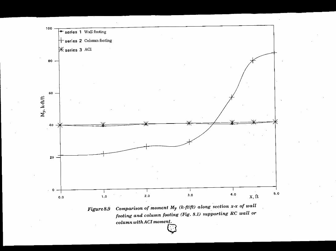
~4:l;:i

100

80

60

40

20

o

series 1 Wall footing

series 2 Column footing

series 3 ACI

0.0 1.0 2.0 3.0 4.0 x,ft5.0

FigureB.9 Comparison of moment My (h-ft/ft) along section x-x of wallfooting and column footing (Fig. 8.1) supporting RC wall or

column withACI moment.n,'-~

8.3 Eccentric Footing

In conventional analysis of rigid footings under eccentric loading, the soilpressure can be computed from principles of mechanics of materials forcombined bending and axial stresses. When footings have moment aboutone axes only, it is a simple exercise to find the centre of base pressure evena part of it is subjected to soil tension. But the solution of such problems withdouble eccentricity needs detail calculation to find the line of zero pressure.A number of solutions in chart form may be prepared4 to estimate the line ofzero pressure. which separate the effective compression zone and thetension zone for footing bases. These usually require considerable study andsome interpolation. Moreover estimation the zero pressure line is not theend. In eccentric footings, determination of critical values of moments fordesign is also difficult particularly when biaxial bending is present. In suchsituation some sort of numerical solution to the problem will be helpful. Thefinite element program development in this study is fully capable ofanalysing these type of eccentric footings.

8.3.1 Numerical Example of Eccentric Footing

Eccentric footing given in Fig. 8.10 is considered under two different cases tostudy 'the. displacement and moments of such footing. Case I and case II aredefined depending on the manner in which the moments. (Mx or My) are'applied. In case I the moments Mx and My, each is divided into eight equalparts and applied at nodes 49, 50, 51, 60, 62, 71, 72 and 73. In case II, themoments Mxand Myare applied as equivalent vertical loads. The equivalentstresses of Mx or My are computed by using the formula Mc/I. Theequivalent vertical loads at nodes are then determined by using shapefunction. In both cases vertical load is uniformly distributed over thecolumn area and applied as equivalent concentrated loads. The idealisationof forces for case I and case II are given in Tables 8.1 and 8.2 respectively.Loaded nodes are considered free to rotate to allow rotation of the footingwhich might occur due to eccentric loading. The displacements wandmoments My of the footing thus obtained are presented in Figs. 8.11 and

8.13.

117

118

5

10

15

25

20

4

9

19

24

1'-4.5"

62 14

N 51

3

23

8

18

N SO

1'-3"

N71

2

7

N49

17

22

12 N60

6

21

11

16

"-0"

"-0"

1 '-0"

1'-3"

1'-4.5"

1'-4.5"

(Data: BXL= 6x6ft,P= 60k, ks= 100 kef, v = 0.15,E = 4.68 x 105 ksf, Mx = My = 120 k-ft).

Figure 8.10 Mesh layout for eeentrie footing.

Table 8.1 Equivalent forces at nodes for case I

Local Particular Vertical load P Moment Mx Moment My

nodes nodes1 49 - P/12 (-5) Mx/8 (15) My/8 (15)

2 50 P/3 (20) Mx/8 (15) My/8 (15)

3 51 -P/12 (-5) Mx/8 (15) My/8 (15)

4 62 P/3 (20). Mx/8 (15) My/8 (15)

5 73 -P/12 (-5) Mx/8 (15) My/8 (15)

6 72 P/3 (20) Mxl8 (15) My/8 (15)

7 71 -P/12 (-5) Mx/8 (15) My/8 (15)

8 61 P/3 (20) Mx/8 (15) My/8 (15)

Table 8.2 Equivalent vertical loads at nodes for case II

Local Particular Vertical loade Eq. Ver. Load Eq. Ver. Load Total

nodes nodes P Px= :tMxl1.25 Py= :tMy/1.25

1 49 - P/12 (-5) -Pxl6 (-16) Py/6 (-16) -37

2 50 P/3 (20) ( 0 ) -2Py/3 (-64) -44

3 51 -P/12 (-5) Px/6 (16) -Py/6 (-16) -5

4 62 P/3 (20) 2Px/3 (64) ( 0 ) 84

5 73 -P/12 (-5) Px/6 (16) Py/6 (16) 27

6 72 P/3 (20) ( 0 ) 2Py/3 (64) 84

7 71 .P/12 (-5) -Px/6 (-16) Py/6 (16) -5

8 61 P/3 (20) -2Px/3 (-64) ( 0 ) -44

119

120

-().( 11(l7

-0.0107(.().()2(Hl)

-O,()47

-0.047l-(l.{):jOj

l.n 14::)0.0145

"

C<'1~W ICns,- IlB()w\f's

[l.172() ('.;'IS'" I(l.1 7~(l C;l.•..t' [IIll. l{i!)) Bl,)\vks

"-0"

20

o.ooa(l.mJ~J(O.nD:31

O.I:1ti0.130'

" 0.0031

~'-

.(l.022

-0.022

24

Theoritical line ofera pressure,

'-.'-~~).()()148.:~U)24

_()~lI48 (Kz2~-n,02\,-(),024

1'.4.5"O.(l8540.0855

7

-0,024-(>.024

,O.()2~

'.~,024

'-

-0.093-0.093

Zero pressure line(FE Analysis)

-0.022-0,022

12

-0.022 0.003!"-0.022 0.0031

-0.104-0.194(.G.20Gl 2

Vertical displacements ofecentric footing (Fig. 8.10) forcase I and case II and compared with Bowles solution.(-) sign indicates soil footing separation.

11

16

, '-0"

-0.267-0.267(-0.2741

"-3 It

"-0" a' , '-4.5" a "-3 It

-0.047 -0.0108 ~0.0145 ....." n.O:3D7

.0.049 -0.0108 ~145, 0.0307

(-0.0501 (-[l.0201

"-0",

, '-4.5"

Figure 8.11

1'-4.5'

-0.05 -0.02 00180.166

11~O!! ,-0.019 0.019

0.093l!~O"

,-0.01 0.020

Theoriti a1 line of

1'-0" zero Presure

-0.05 -0.017 201'"0"

,

.0.127 -016 0.0211'_Oll (j) @ @)

.0.200 .0.021'_011 @ @ @ @

-0274 1'_0" l'eD" 1'-0" 1'_0" 1'.0" 1'-0" -0.05

Figure 8.12 Displacements obtained by Bowles4 of ecentric footing (Fig.B.1O).

In Fig. 8.11 the vertical displacements are shown for case I and case II andcompared with Bowles solution. Fig. 8.12 shows the vertical displacementsobtained by Bowles4 in some more details. It is observed that both case I andcase II gives almost identical vertical displacements and shows goodagreement with Bowles solution. It is also observed that the verticaldisplacements obtained in the present study are more consistent in naturecompared to Bowles solution. In the present study the line of zero pressureoccurs along line a'c'. But in Bowles solution it is difficult to draw a singleline of zero pressure due to inconsistent displacement variations.Comparing the displacements of two extreme points i.e. points P and Q, it isfound that the line of zero pressure a'c' is compatible with thedisplacements of the footing. The line of zero pressure (a'c') shifted slightlyfrom its theoretical4 position (ac) because of the elastic deformation of thefooting. In the theoretical analysis the footing is assumed to be perfectly

rigid.

121

122

Figure 8.13 Moments My (k-ftlft) of eccentric footing (Fig.B.10) for case Iand case II.

Case ICase IIxlCase ICase II

x

y

y

0.92 2.05 1S5 343 168 164

197 3.54 386 152 2.61 3.800

4.30 16.07 1731 7.74 5.73

4.35 11.55 11.45 9.22 7.82N72 N73 6.92

426 5.29 8.30 19.73 15.86 2285 1211 831 7.47

340 3.98 8.45 17.58 26.79 27.79 18.64 12.05 10.80 0

3.76 3.61 8.76 10.85 11.63 992 8.39 7.22

122 137 1.85 1099 1877 1541 10.72 985N49 N'O

2.92 2.25 158 - 520 342 -121 7.30 802 7.53

-0.83 137 -479 - 9.91 .7.24 117 7.28 9.38 894

@ (f) @ @ @J

3.16 -0.05 -143 1.27 2.61 2.02

-0.83 -0.93 0.48 -0.77 112 0.98

G) @ @ @ @

x

xl

The moments ~ for case I and case II are presented in Fig. 8.13. It is

found that for both cases the maximum positive moments occurs along

section x-x while the maximum negative moments occurs along section x'.

x'. It is also found that moments obtained both cases are comparable.Comparing the moments for both cases at section x-x and x'.x' (particularly

at nodes 49, 50, 51 and 71, 72, 73) it is observed that the moments obtained for

case II are more acceptable. Therefore case II may be considered better

model in applying moment.

8.4 Pile Foundation

In conventional method, the distribution of applied forces to individual pilesis determined from combined stress equation. This assumes the pile cap asinfinitely rigid. But the term 'infinitely rigid' is impractical and capflexibility would playa significant rule for distribution of applied forces toindividual piles. The finite element program developed in the study iscapable of analysing pile foundation. However its use is limited to the casewhere the piles, and cap loads are vertical and only Mxor My(or both) arepresent. In the program there is provision for including the vertical as wellas rotational stiffness of piles. Therefore in using the program in addition topile loads, pile moments can be obtained automatically. To study theperformance of the program the following numerical example is

considered.

8.4.1 Numerical Example of Pile Foundation

A pile foundation shown in Fig. 8.14 is analysed with the present finiteelement program for two different cap rigidities. The example is taken from.Ref. 4 for the purpose of comparison. In computing rotational stiffness ofpiles, A2 and AS (as defined in sec. 3.7.5) is taken as 2.0. At first the cap isanalysed with the normal. modulus of elasticity (Ee =2.65 x 107 Kpa) ofconcrete (Case 1). In order to make the physical behaviour of the capunderstandable and for ease of comparison with Bowles solution4, the caprigidity is then increased about 100 times (case II). The results thusobtained are presented in Figs. 8.15 through 8.18 and compared with Bowlessolution. The comparison of pile loads and pile moments are also given intables 8.3 and 8.4 respectively.

Comparing the vertical displacements as well as the pile loads from Figs .. 8.15 and 8.16 it is observed that cap rigidity plays an important role fortransfer of column load to individual pile. When the cap relatively flexible(i.e. case 1) pile-5 experiences the largest vertical load due to the largestsettlement of this point. However, when the Ec of the cap is increased to 100times the normal Ec, the cap behaves almost like a rigid mat. The verticaldisplacements and pile loads obtained for this situation are all comparableand identical with those of Bowles. For this rigid cap the pile loads are alsofound almost identical with those obtained using conventional method

123

124

8 x

7

@

16

12

0.7

11

15

0.7

4

5

6

14

0.7

CD

13

@

Figure 8.14 Mesh layout for pile foundation

0.7

1

x 2

0.6

0.6

x' 3

0.6

0.6

(pile data: E = 200,000 Mpa, Ix= 508 x 10-6 m4, Iy= 184 x 10-6m 4,

A=22.2x10-3m2, L=19.00m, /"FO.50

Cap data: Ec = 26500 Mpa, t = 0.60m, v = 0.15, P = 7200 KN at centre,Mx = 500 KN-m, ks= 0.0, Assuming /"2= "3 = 2.0)

125

Figure 8.15 Comparison of vertical displacements w (fr) of pile foundation(Fig. 8.11:) for case I and case II and Bowles4 solution.

0.007210.00731(0.0073)

0006390.00730(0.0073)

0.00729 Case I : Ec=2.65x1070.00731 Case II . E = 2 65x109(0.0073) Bowles . E~ in 'Kpa .

(0.0068)(0.0064)

0.00630 0.00777 5 0.00916 0.00832 80.00639 0.00663 .0.00687 0.00709(0.0064) (0.0068)

@ @ (J) @

0.00622 0.00751 000831 0.008050.00638 0.00663 0.00687 0.00709(0.0064) (0.0068)

(j) @ @ @0.00551 0.00702 0.00755 0.00751000638 0.00662 4 0.00686 0.00701 71

2

The pile moments are shown in Fig. 8.17 and Table 8.4. It is found that thepile loads and the pile moments of both ease I and ease II satisfy the over allcondition of equilibrium. However in the present study the pile momentsobtained are very small compared to Bowles solution. It is to be noted thatthe pile loads and pile moments of Bowles solution do not satisfy the over allcondition of equilibrium. Besides as shown in Figs. 8.16 and 8.17 pile loadsand pile moments obtained by Bowles produce zero moments at sections xxand yy of the pile cap. The moments Mx and My of the pile cap are shown inFig. 8.18 and found that the total moments at sections xx and yy for ease Iare 2608.20 KN-m and 2974.38 KN-m respectively. This also shows goodagreement with pile reactions of ease 1. In ease II where the cap behaveslike rigid mat the total moment (My) at section xx is 2874.11 KN-m. Addingthe negative moments of pile, total moment in the y direction for ease II is2875.64 KN-m. In Bowles solution total moment obtained in the y direction is2880 KN-m which is very close to the value obtained hear in ease II.However, the total moment of Bowles soution is entirely carried by pilesleaving zero moment at section xx. This is obviously incorrect andthe .inconstancy in the formulation of Bowles, lies in his assumption that

(Table 8.3). Moment Mx produces the larger vertical loads on piles 7, 8 and9 compared to loads on piles 1, 2 and 3. This effect of moment on pile loaddistribution is observed in both eases of cap rigidity considered.

FigureB.16 Comprison of pile reactions (KN) for case I and case II andBowles4 solution.

FigureB.17 Comparison of pile moments (KN-m) for case I and case IIand Bowles4solution.

126

Table 8.3 Comparison of pile head loads (vertical), KN

Pile Pile loads with pile Pile loads assuming rigid pile cap %

No cap of actual concrete. FE Analysis Bowles Convention variationFE Analysis al method (5-2)

1 2 3 4 5 61 643 745 745 740 ~132 736 746 745 740 01

3 643 745 745 740 0134 882 801 800 800 -105 1070 803 800 800 -346 882 801 800 800 -107 746 853 855 860 (,>138 851 854 855 860 01

9 746 853 855 860 013

Table 8.4 Comparison of pile head moments, KN-m

Pile Pile loads with pile Pile loads assuming rigid pile capNo. cap of actual concrete FEAnalysis Bowles

Mx Mv Mx Mv Mx Mv

1 30.1 36.7 5.4 0.5 1038.8 894.02 29.9 0.0 5.4 0.0 1038.8 0.03 30.1 -36.7 5.4 -0.5 1038.8 -894.04 5.8 41.2 5.1 0.5 -4.3 960.05 14.0 0.0 5.2 0.0 -4.3 0.06 5.8 -41.2 5.1 -0.5 . -4.3 -960.07 -21.9 . 40.0 4.8 0.5 -1201.2 1026.08 -20.3 0.0 4.8 . 0.0 -1201.2 0.09 -21.9 -40.0 4.8 -0.5 -1201.2 -1026.0

127

FigureS.IS Pile cap moments (My and MJ for case I and case II.

15.7216662

.102870

.13029

-41.07 Case I32.32 Case II

-13802118.20

53717681.88

x'465.00 Case I557.92 Case II

88474

596351

-72.18-110.61

128

Y901970

-97.522546

Y 929.38

(b) Moment Mx (KN-m /m)

(a) Moment My (KN-m/m)

81645

31808

-51.59-88.14

9540-~ ~ ~47.69 38971 2188.90 5373.70

@ @ 155820 IJ) @

171170

-52.91 521.43 1097.00 707.72

-78.74 630.63 123500 8225

CD @ 914.27 @ @)1082.60

-77.53 722.19 755.96 78754

62.51

-1022613397

x407.20 56929 735.95 1203.50 177980 132650 78501 615.9749260 670.30 81273 129800 1981.80 142480 864.88 724.46

@ @ IJ) @

513.92 401.69 296.50 461.75626.58 48269 338.87 547.70

CD @ @ @)

the pile cap is absolutely rigid. By absolutely rigidity he meant that theexternal forces and moments, will be entirely carried by the pies while thepile cap merely connects the piles as a rigid plate. For case I (whichrepresents the actual behaviour) it is found that the relative stiffness of thepiles of section x'-x'(Figure 7.13) is only 2.5% of the pile cap and pilesmoments are about 4.3% of the total moment in the y direction. Since thereis approximation in determining the above relative stiffness, piles momentsobtained in the present study may be considered satisfactory.

8.5 Mat Foundation

The approximate flexible method is suggested by ACI committee 3361

fordesign of mat foundation. Shukla2 recommends this method to calculatemoment, shear forces and deflections of mat foundation. To compare theperformance of this method the following numerical example is considered.The conventional method of mat design is also included for comparison.

8.5.1 Numerical Example of Mat Foundation.

The numerical example of mat foundation given in Fig. 8.19 is taken fromRef. 2 for the purpose of comparison. The mat supports 16 columns. All thecolumn are 18 x18 in. in cross section and are spaced at 15 ft each way: Theedge distance of the mat from the centre line of the end column is 3 ft. Thefour central column carry a total load of 300 kips each, the corner columncarry 150 kips each, and remaining edge columns carry 200 kips each. Thetotal depth of the mat is taken to be 2.0 ft from consideration of punchingshear. The ks value of mat soil is given as 28.44 klft3. It is to be noted thatplate rigidity calculated in the above mentioned reference is in error and thevalue given is about 12 times less than the actual value. To obtain identical L(radius of influence) value, the ks value is also increased 12 times and takenas 341.28 klft 3. The moments Mx and My obtained with present finiteelement analysis are compared with those obtained using approximateflexible method and conventional method in Table 8.5.

With present finite element analysis the maximum negative and positivemoments are found to be -26.60 and 43.93 k-ftJft and occurred at points 8 and9 (Fig. 8.19) respectively. From Table 8.5, it is seen that the positive moment

129

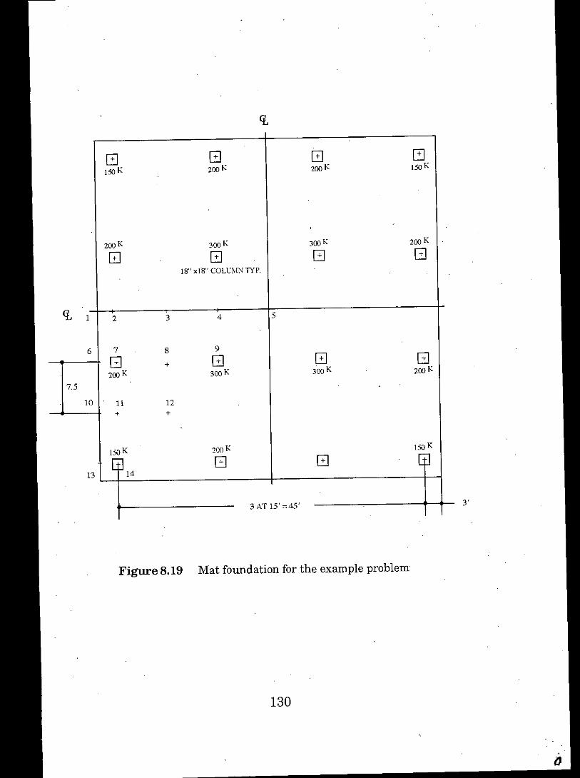
G G G ~150K 200K 200K 150K

200K 300K 300K 200K .

0 G G G18" xfS" COLUMN TIP.

CL 1 2 3 4 5

6 7 8 9

G + G G G200K 300K 300K 200K

7.5

10 11 12+ +

150K 200K 150K

4114

G G13

3 AT 15' =45'

Figure 8.19 Mat foundation for the example problem

130

3'

obtained with conventional method is very small compared to the maximumpositive moment of finite element analysis. However, negative momentobtained with this method are comparable with the maximum moment ofFE analysis. The maximum positive moment using approximate flexiblemethod is found 21% greater than that of FE analysis. The maximumnegative moment using this method is found to be about 8% higher, whilethe negative moments at other portion of the mat are found significantlylower compared to the corresponding values of FE analysis. Using thisflexible.method the column face moment of point 9 is found to be 2% less atleft face and 12% less at right face. It is to be mentioned here that columnface moment calculated by the author at the faces perpendicular to the.direction of moment, while in Ref. 2 it is calculated at faces parallel to the

direction of moment.

Table 8.5 Comparison of Moments for Mat Foundation

Location Moment Conventional Approximate FE Analysis % variationFig. 8.19 Mx arMy Method flexible method!.2

ks=341.30 ks=341.30 (3-5) (4-5 )

1 2 3 4 5Point 4 Mx 8.0 7.5 6.1 32 24

My -25.0 -7.2 -15.3 63 -53

Point 5 Mx -25.0 -3.8 -8.5 193 -55My -25.0 -3.8 -8.5 193 -55

Point 8 Mx -28.0 -28.6 -26.6 5 8My 8.0 5.4 .2.0 . -

Point 9 Mx 8.0 53.0 43.9 -82 21My 8.0 53.0 43.9 -82 21

column Mx,LF 4.5 32.8 33.5 -87 -2face of Mx,RF 4.8 32.8 37.2 -88 -12point 9

131

8.6 Comparing the performance of Shape Function and ContributingArea Methods in Calculating Node Springs and the Effect of SelfWeight of Foundation

As discussed in sec. 3.7.2 both shape function and contributing areamethods can be used to compute node springs from subgrade reaction.When shape function is used the system may. be considered moreconsistent. However as soil tension is not permitted where soil separationoccurs this method will not be applicable.

In order to compare the performance of the above two methods the bendingmoments (My) and vertical displacements of spread footing of Fig. 8.5b arepresented in Fig. 8.20a. It is seen that for both methods the verticaldisplacements and bending moments are almost identical. But for gravityload uniformly distributed over the mat area, it is observed that shapefunction method provides perfectly uniform displacement even for veryflexible mat as shown Fig. 8.20b. However, displacements obtained usingcontributing area method for flexible mat have the oscillating tendency (Fig.8.20b). Since foundations are normally rigid, in actual foundation analysisthis does not make any difference and both methods can be usedconveniently. However, where soil separation occurs contributing area

.method is essential.

In structural analysis of foundation the self weight is not usuallyconsidered since it is assumed to be supported directly the underlying. Asshown in Fig. 8.20b, it is found that distributed loading produce negligiblemoment in the footing. Therefore it is not essential to include self weight instructural analysis of foundation. However, where there is a possibility ofsoil separation it should be considered.

132

FigureB.20 Comparison of moment My (k-ft / ftJ and vertical displacementw (ft) for column footing (Fig. 8.5) obtained using shapefunction and contributing area methods.

(b)Distributed loading

0050000.04989

o 05000004975

0.050000.04997

0.050000.05021

0.050000.05036

0.050000.05007

0050000.0504.2

0.050000.05011

0.050000.05043

0.00 0.050000.18 0 04930

Ec=1.17x103 ksfw0.05000 SF0.05011CA

25

My My

o 181 000 SF018 0.04 CA

20

0183 0.00 SF0.18 0.066CA

15

0182 0.000.18 011

@

0.183 000o 18 0.16

@

.

Ec=4.68 x105 ksf

o 05000 0 185005000 0.18

0.050000.05000

0050000.05000

0.050000.05000

0.050000.05000

0.050000.05000

0050000.05000

005000005000

0.05000005000

133

wSF005000CA005000

w

0.05082 SF0.05085 CA

25 0.05080My My 0.05080SF CA

78.28 78.45 0.05073005075

20 0.050630.05064

3069 30.89 0050510.05051

15 0.0503800538

1063 1084 0.05024o 05025

@ 0050110.05011

1.74 1.93 0.04998004999

@ 0.049860.04987

0049750.04975

(a) Concentric loading

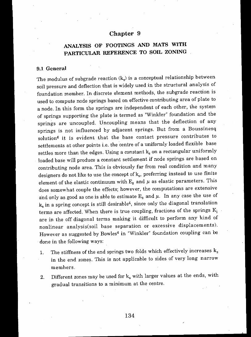
Chapter 9

ANALYSIS OF FOOTINGS AND MATS WITHPARTICULAR REFERENCE TO SOIL ZONING

9.1 General

The modulus of subgrade reaction (ks) is a conceptual relationship betweensoil pressure and deflection that is widely used in the structural analysis offoundation member. In discrete element methods, the subgrade reaction isused to compute node springs based on effective contributing area of plate toa node. In this form the springs are independent of each other, the systemof springs supporting the plate is termed as "Winkler" foundation and thesprings are uncoupled. Uncoupling means that the deflection of anysprings is not influenced by adjacent springs. But from a Boussinesqsolution4 it is evident that the base contact pressure contributes tosettlements at other points i.e. the centre of a uniformly loaded flexible basesettles more than the edges. Using a constant k.,on a rectangular uniformlyloaded base will produce a constant settlement if node springs are based oncontributing node area. This is obviously far from real condition and manydesigners do not like to use the concept ofk." preferring instead to use finiteelement of the elastic continuum with Es and Jl as elastic parameters. Thisdoes somewhat couple the effects; however, the computations are extensiveand only as good as one is able to estimate Es and Jl. In any case the use ofk., in a spring concept is still desirable4, since only the diagonal translationterms are affected. When there is true coupling, fractions of the springs Kiare in the off diagonal terms making it difficult to perform any kind ofnonlinear analysis(soil base separation or excessive displacements).However as suggested by Bowles4 in "Winkler" foundation coupling can be.done in the following ways:

1. The stiffness of the end springs two folds which effectively increases ksin the end zones. This is not applicable to sides of very long narrow

members.

2. Different zones may be used for ks with larger values at the ends, withgradual transitions to a minimum at the centre.

134

9.2 Relative Stiffness Parameters

Prior to the presentation and discussion of the results it is appropriate todefine a relative stiffness parameter for the plate elastic foundation system.A number of such parameters can be chosen. In the present study weadopted the relative stiffness parameter Kr for spread footing defined byGorbunov SerebIjanyi26 i.e.

Kr={l21t (l-vp) 1(1-vs2)}(EslEc)(lIt)2(b/t) (9.1)

and as suggested Bowles4 when k" is substituted for E/2b(1-vs2) the aboverelation becomes

Kr= 241t(l-v p) (k/Ec)(l!t)2(b2/t) (9.2)

where 21,2b and t are respectively the length, breadth and thickness of therectangular plate. The limiting case of rigid mat is obtained when

Kr:s;8/(lIb) 0.5 (9.3)The above relative stiffness parameter should not be used for strip footing ormat foundations, because the expression does not include the effect ofcolumn load and column spacing. The expression only tells larger footingshave greater flexibility. ACI committee 436 (1966)1 suggests that in acontinuous strip if the average of two adj acent span does not exceeds 1.75/Aand also that the adjacent span and column loads do not differ by more than20 percent of the larger value, the foundation is regarded as rigid

LfkiHere, A = -\j'4Ec!J (9.4)

wherek".= Sk'sk's =,coefficient of subgrade reaction as defined in soil mechanics, kef.b = width of the footing, ftI = moment of inertia, ft4Ec = modulus of elasticity of concrete, ksfS = shape factor

= [(b+1)/2b]2 for granular soil such as sands= (n + 0.5)/1.5n for cohesive soil such as clays, where n is the ratio of thelonger to shorter side of strip.For mat foundation if the column spacing is less than l/A, the structuremay be regarded as rigid.

135

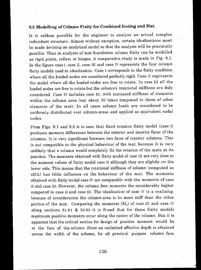
9.3 Modelling of Column Fixity for Combined footing and Mat.

It is seldom possible for the engineer to analyse an actual complexredundant structure. Almost without exception, certain idealisations mustbe made devising an analytical model so that the analysis will be practicallypossible. Thus in analysis of mat foundation column fixity can be modelledas rigid joints, rollers or hinges. A comparative study is made in Fig. 9.1.In the figure case I, case II, case III and case IV represents the four columnfixity models used in idealisation. Case I corresponds to the fixity conditionwhere all the loaded nodes are considered perfectly rigid. Case IIrepresentsthe model where all the loaded nodes are free to rotate. In case III all theloaded nodes are free to rotate but the column's rotational stiffness are duly.considered. Case IV includes case III, with increased stiffness of elementswithin the column area (say about 10 times compared to those of otherelements of the mat). In all cases column loads are considered to beuniformly distributed over column-areas and applied as equivalent nodalnodes.

From Figs. 9.1 and 9.2 it is seen that fixed rotation fixity model (case I)produces moment differences between the exterior and interior faces of thecolumns. It is very significant between two faces of interior columns. Thisis not compatible. to the physical behaviour of the mat, because it is veryunlikely that a column would completely fix the rotation of the mats at itsjunction. The moments obtained with fixity model of case III are very close tothe moment values of fixity model case II although they are slightly on thelower side. This means that the rotational stiffness of column (computed as4EIIL) has little influence on the behaviour of the mat. The momentsobtained with fixity model case IV are comparable with the moments of caseII and case III. However, the column face moments the considerably highercompered to case II and case III. The idealisation of case IV is a realising,because of consideration the column-area to be more stiff than the otherportion of the mat. Comparing the moments (Mx) of case III and case IV

along sections Xl-Xl & X3-X3 it is found that for these fixity modelsmaximum positive moments occur along the centre of the column. But it isapparent that the critical section for design of positive moment would beat the face of the column. Since an unlimited effective depth is obtainedacross the width of the column, for all practical purpose column face

136

(f

<i:

X310.0 163980.48 26-,67 64,08 4.74 -68.6521.9863.60 68.42 47.95 -30,71 -90,7220.8962.90 68.12 48.79 -26.71 -88.5923.01 79.29 64.25 52.96 -23.2.1 -84.33

i 23.93 20.9023.32 11Al23.93 13,4819.57 11.82

-72.&7-95.91-93.72-89.19

-14.24 14"7.61 229.99 41.l~ 136.48 73.82-41.47 74.43 225.98 254.59' 228.76 84.06.39.60 79.71 224.14 247.70 224.68 81.18-30.44 99.70 308.37 361.72 316.72 102.64

137.37 120.20144.04 146.95145.28 145.79131.41 131.74

.32.02 .-25.13-26.57-15.91

I' - 6"X 3 •.~..•.1

.66.70 Case r-59.61 Case II-60.91 Case III-53.55 CaseIV

"5"- 0"

<i:

X21o.o + -3.58 f1317 rl9 r88 t 9.82 r6 r80 f81 -38.39tX20.0 -7.24 -21.71 .60,90 -64.18 .8.94 53.90 57,09 11.53 -21.83 6':0"-6.68 -2037 -58.89 -61.99 -6.25 54.94 56.94 9.93 -23.83-6.81 -20.05 -58.45 -61.29 -6.19 52.56 54.79 11.42 -ZI,(l4

XI

6.495.145.683.58

14.6930.38

CD 30.9234.84

3'.0"

-0.91-7.66

I I I81.80

-5.9783.03

-7.2584.9074.82

19.41 -15.89 -56.20 -56.57 -6.68 97.33 144.72 36.07 I-as.12.10 -35.47 -73.61 -76.34 -28.53 40.51 127.71 51.23 -102713.10 .32.23 -70J~4 -74.02 -27.03 46.88 126.48 47.34 -12.0511.50 -31.44 -69.13 -71.74 -22.68 58.17 171.41 61.51 -7.01

29.11150.92 80.6717.10142.39 145.43@ 118.10 @ @ @ @ 139.70 (j) 142.89 @ I @19.93177.33 191.33

2'.0" 4'- 6" 4'- 6" 4'- 6" 4'- 6" 2' - 0" 4' .6" 4'.6"

5' - 0"

-51.76) X I-38.49-4OAI 3'.0".35.46

3'.0"

Figure 9.1 Comparison of moments Mx (k-ftlft) of mat foundation (one-fourth of the mat shown) for four different columnfixity models, case I, case II, case III and case IV. ..:

(Data: t = 3'-0", Ec= 4.68x 105, 4.68x1rJ', 1.17x10", v = 0.15, PI = 450k, P2" 90ok, Pa'= 45ok, P4= 900k)

137':"

<i:

~~~

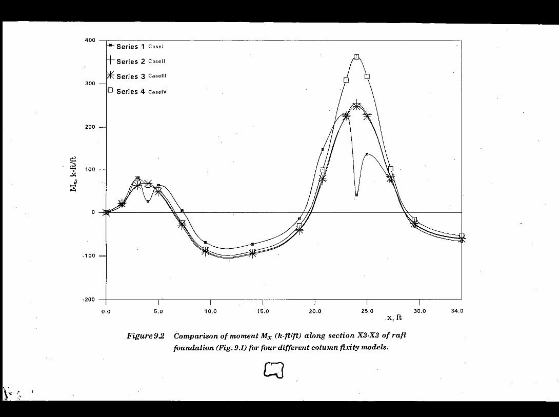
i

400

300

200

100

o

-100

-200

Series 1 Case I

Series 2 Casell

Series 3 Caselli

Series 4 CaselV

0.0 5.0 10.0 15.0 20.0 25.0x, ft

30.0 34.0

,

Figure 9.2 Comparison of moment Mx (k-ftlft) along section X3.X3 of raftfoundation (Fig. 9.1) for four different column fixity models.

CJ

moments could be safely used for design. If the centre line moment is usedin proportioning the mat thickness an. unnecessary thick section wouldresult. The above column fixity models may be examined for strip footing aswell. Case I, III and IV have been employed for such a study of strip footingsupporting three columns. One-half of the footing is shown in Fig. 9.3 alongwith the results obtained for three fixity idealisation. From Fig. 9.3 it isfound that an abnormally large moment develops at the face of exteriorcolumn for Case I, while it underestimates the negative moment at thecentre span. On the other hand in case III positive moment obtained at thecolumn face of interior column is comparatively small. Comparing themoments of case I, case III and case IV of Fig. 9.3, it is observed that like raftfoundation the moments of case IV are more acceptable for strip footing. Forspread footing since symmetry exists around the column, case I mentionedabove is a more realistic model. However even fixity modelling of case IVdiscussed above can also be used. This has been already discussed withexample in Chapter 8.

139

Figure 9.3 Comparison of moments My (k-ft / ft,) of strip footing for threecolumn fixity models, case I, case m and case IV.

(Data: P1=540k, P2=540k, Ec =4.68x J(P ksf, v=0,15, ks=100kcf for allelements, one-half of the footing shown,)

4' - 0"

140

Y 004782102 26

2' • 0"Y N92

4' .0"

64.89 - ();oo ••.•P299.21 170 92 197.6'1'75.91 27816 ~~]~p l' - 6"

67.50 - 22336 Case I96.63 13253 138.32 Case III7105 196.07 24930 Case IV 2' - 0"

N70 .

6975 69584458 24.685196 49.26

4' - 0"

N59

-49 57 -57 95-85.11 -90 62-7849 -85 88

4' - 0"N48

-89 69 -9171 4-142.37 -146.87-14193 -143.25 4' - 0"

N37

-5193 -64.23-14009 -14550-138.54 -143.28

4' - 0"(J) @ @

N26

63.33 76.52-5236 @ -7307 @-54.17 -6711 2' - 0"

N.l51113 - '288,64 PI-5.54 CD3871 .9:71 @-1624 31.54 17,94 l' - 6"

-t{4

500

400

300

Series 1 Case I

Series 2 Caselli

Series 3 Case IV

~~~

i

200

100

o

.100

-200

0.0 5.0 10.0 15.0

y, ft20.0 23.0

,

Figure 9.4 Comparison of moment My (h-ft/ft.) along section y.y ofstrip footing for three different column fixity models

141

9.4 Effect of Soil Zoning on Foundation Behaviour

One of the main objectives of present study was to study the effect of soilzoning on the behaviour of footings and mats. Here two cases areconsidered. Foundation analysed with constant ks value i.e. single ks valuethrough out the foundation is identified as case 1. Case II defines thecondition of soil zoning i.e. the area under the foundation is divided intothree zones and three different ks values are considered. The relativestiffness parameters defined in sec. 904 are varied by changing singleparameter Ee and the analysis are carried out with different foundationrigidities for both cases. Types of foundation considered in the studyincludes spread footing, strip footing and mat foundation. Their behaviourare separately discussed below for both cases mentioned above.

9.4.1 Spread Footing

To study the effect of soil zoning, a square footing shown Fig. 9.5 isconsidered. In case I a constant ks of 100 kcf is used, while in case II three k,value of 125.00,93.75 and 62.5 kcf are considered for three zones marked inFig. 9.5. These three ks valus are so selected for three zones so that theweighted average of the ks values becomes 100 kcf. The relative stiffnessparameter Kr is varied by changing Ee values and four different Ee valuesare considered for both cases. Among them, Ee equal to 4.68 xl05 ksf is thenormal Ee of concrete while other three reduced values are considered justto make a comparative study, To'model the footing 8 noded element is used.The applied load is uniform by distributed over element 25 (Fig. 9.5) andapplied as equivalent vertical loads. The rotations of loaded nodes areconsidered fixed. The vertical displacements w at section Xl-Xl andmoments My at section X-X thus obtained are presented in Fig. BA ofappendix B with different footing rigidities for both case I and case II. Thegraphical comparison of vertical displacements wand monents My aregiven in Figs. 9.6 and 9.7 respectively.

If the footing were perfectly rigid the uniform displacement for both caseswould be 0.050ft. As shown in Figs. BAa and 9.6, when the footing isrelatively rigid one, the displacements obtained for both case I and case II

are almost identical and very close to the uniform displacement. Howeverwhen the footing rigidity is decreased the displacement variation is

142

~Figure9.5 Mesh layout and soil zoning for spread footing. One-fourth of

the footing shown.

(Data: b=5'.0", t = 2'.0", Ec=4.68x 105, 7. 19x1()4, 2.88x104, 1.15x104 hst;

v=0.15,P/ 4= 125h.)

observed for both cases. For relatively flexible footing i.e. increasing Kr to 8.20 and 50, the differences of edge and central displacements for case I arefound to be 13.7%, 33.1% and 76.5% respectively. For case II these differencesare 15.1%, 36.8% and 86.8% respectively. Therefore, as shown in Fig. 9.6 thedisplacement variation is found to be significantly influenced by the footingrigidity for both case I and case II.On the other hands the variation of therelative displacement between the edge and centre of the footing is lesssensitive to zoning effect (case II) compared to case 1.Moreover from Fig. 9.7it is observed that the moment variations are not the very significant withthe displacement variation. Changing Kr from 1.2 to 50.0 it is found that thedifference of edge and central displacements increases about 36 times f()rcases I, while the reduction of maximum moment is only 9.4'7r. As themoment variations are not very sensitive with displacement variation, soilzoning suggested by Bowles may not be considered for spread footinganalysis.

143

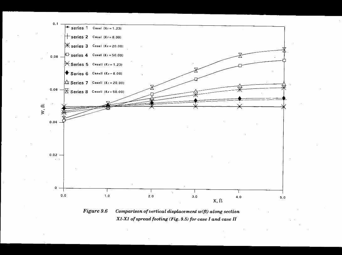
0.11 Casel {Kr = 1.231

Casel (Kr= 8.001

CaseIIKr=20.00J

0,08 1......../ ::;~II~::;""t Casel (Kr = 50.00)

Casell I Kr = 1 .231

Casell (Kr= 8.00)

Casell (Kr = 20.00)

0.06 t Series 8 Gasell (Kr=50.001

V'~4::~-

0.04

0.02

o0.0 1.0 2.0 3.0

x,ft4.0 5.0

Figure 9.6 Comparison of vertical displacement weft) along section

XI.XI of spread footing (Fig. 9.5) for case I and case II

100series 1 Casel IKr::= 1.231

series 2 Casel IKr = 8.00)

series 3 .Casel IKt=20.00J

80 L-, series 4 Casel (Kr = 50.00)

Series 5 easel! IKr = 1.231

Series 6 Gasell IKr= 8.00)

Series 1 easel! IKr = 20.001

60 -1£ .Series 8 CaseJl IKr=50.00)

~;;:;,~~>.

40

20

o0.0 1.0 2.0 3.0 x, ft. 4.0 5.0

Figure 9.7 Comparison of moment My(k-{t/{t) along section X-Xof spread footing (Fig. 9.5) for case I and case II

145

9.4.2 Strip Footing

To study the effect of soil zoning on foundation behaviour, strip footingshown in Fig. 9.8 is considered next. The footing supports three columns.For better understanding of the physical behaviour of the footing, exteriorcolumn load is taken half of the interior column load and loaded nodes areconsidered fixed. To analyse the footing 8 noded element is considered. Theapplied loads are uniformly distributed over elements 2 and 23 and appliedas equivalent vertical load. The footing analysed with constant ks of 100 kefis identified as case 1. Case II defines the condition of soil zoning i.e. thearea under the footing is divided into three zones as shown in Fig. 9.8, threedifferent ks values of 133, 100 and 67 kef are considered for these threezones. The ks values are selected in such a way so that the weighted averagevalue of ks becomes 100 kef. The relative stiffness parameter A ( defined byEq. 9.4) is varied by changing Ec of the footing and four different footingligidities are considered for both case I and case II.According to Eq. 9.4, thestrip footing of Fig. 9.8 would be rigid if A .:5. 0.097. Using kg value of 100 kefand footing thickness of 2 ft. together with the four Ec values of 9.8 x105,4.73x105, 1.94x105, 1.21x104 ksf, the values of I, from Eq. 9.4 are obtained as0.063,0.075,0.094 and 0.188 respectively for granular soil. For cohesive soil,they are found to be 0.078,0.094,0.117 and 0.235 respectively. Comparing theA values for both soils with rigid footing I, of 0.097 it is evident that at leasttwo Ec values i.e. 9.8x105 and 4.73x105.ksf(Ec= 4.73x105 ksf corresponds topractical modulus of elasticity for normal concrete) keeps the i, valueswithin rigid footing range, while for other Ec values, A corresponds toflexible footing behaviour. The vertical displacements wand moment M).along the centre of the footing are shown in Fig. B.5 of appendix B. Thegraphical comparison of the vertical displacements wand moments My aregiven in Figs ..9.9 and 9.10 respectively.

Form Fig. 9.9 it is found that for all footing rigidities of case I, the edgedisplacements are slightly greater than those of the central values. Butwhen softer springs are placed near the centre (case II) the behaviour of thefooting is changed. For this situation the displacements and moment valuesbecome higher at the centre compared to the edges. However when thefooting is relatively rigid CEc=9.8x105kilt), presence of the soft springs at thecentre which tends to produce more settlements at this location, force the

146

Figure9.8 Mesh layout and soil zoning for strip footing. One-half of thefooting shown.

18 4'-0"

y

14 15

kg = 5017

k.=7511

16

y4' - 0" 2' - 0" 4' - 0"

22 P2 24

19 20 21 2' - 0"

147

Pi =540k, P2 = 540k, Ec = 9.80x1C5, 4. 73x1C5, 1.94x1C5 and1.21x1()4, ksf t = 2'-0", v= 0.15)

(Data:

o

0.2

I.••...series 1 Case I IE"" 9.80E05)

+Series 2 Case I IE = 4 ..73E05)* Series 3 Casel IE = 1. 94E05J0.15 -1

D Series 4 Casel. IE = 1.21 E04J

~ Series 5 Casel!. IE = 9.80E051

-+- Series 6 easel! IE = 4. 73E05)

0.1 -.j"- \ & Series 7 Casell IE = 1.94E051

tt Series 8 easel! IE = 1.21 E04)<l:: I , ,:;::-

0.05

-0.05

0.0 5.0 10.0 15.0y;ft

20.0 23.0

Figure 9.9 Comparison of vertical displacement weft) along section

y.y of strip footing (Fig. 9.8) for case I and case II withdifferent footing rigidities

148

400I

...•..series 1 Casel IE:= 9.80E05)

+Series 2 Casel (E::=4. 73E05)

300 --I -+- * Series 3 Casel IE:= 1.94E051

D Series 4 Casel IE"" 1.21 E04J

~ Series 5 easel! (E:= 9.80E05)

200 "I f\\ .• Series 6 Casell IE =. 4. 73E05)

:6.. Series 7 easel! IE = 1.94E05)

~ Series 8 easel! IE:= 1.21 E04)I 4\ \\\ \\

100

~~~~>. 0

-, 00

-200

0.0 5.0 10.0 15.0y,ft

20.0 23.0

Figure 9.10 Comparison of moment My(k.ftlft) along section y.y

of strip footing (Fig. 9.8) for case I and case II withdifferent footing rigidities

149

footing to behave partially as simply supported beam supported at the edges.This would lead to transfer a part of the central column load to the edges.Thus for relatively rigid footing, displacements obtained (Fig. 9.9) for case II

are comparable to those of case I. But the moment values at the central.column face for case II are higher due to beam action discussed earlier. Butas the footing rigidity is reduced, it gradually becomes incapable to transferthe central column load to far ends, rather the effect of soil zoning becomeslocalised. As shown in Fig. 9.9, for relatively flexible footing (Ee=1.21x104

ks£) the edge displacement of case IIbecomes 16.7% less than that of case I,

while the central displacement become 28.6% larger for case II. Since the ksvalue near the edge is greater for case II, comparatively smalldisplacements are required to accommodate the load at this location. Butnear the centre the ks value for case II is smaller compared to case I, andcomparatively larger deflection occurs 'at this location to accommodate .theload. For relatively rigid footing (Ee=9.8x104 ks£) they were 8.4% and 11.::;'/,respectively. Therefore footing rigidity plays an important role to influencethe relative displacement of various points. On the other hand the increaseof interior column face moment for case II ( than those from case IJ alsorelated with footing rigidity. As shown in Fig. 9.10 relatively rigid footing(Ec=9.8x105 ksfJ the increase of interior column face moment is found to be48.6%, while for flexible footing (1.21x104) it is found 26.0%. Therefol'e forstrip footing the effect of soil zoning on moment is found significant.

9.4.3 Raft Foundation

Lastly a raft foundation shown in Fig. 9.11 is considered to study the effect ofsoil zoning on foundation behaviour. Like spread or strip footing, case I

defines the condition when the raft is analysed with constant ks of 100 kcf.Case II defines the condition when the area under the mat is divided intothree zones and three different ks values of magnitude 118.56, 88.92 and59.28kcf are considered for the three zones. The zone boundary along withrespectiye ks values are shown in Fig. 9.11. The ks values are taken in sucha way that their weighted average becomes 100 kef. The relative stiffnessparameter J, given in Eq. 9.4 is varied by changing Ee values where threedifferent Ee values of 4.68xl05, 4.68xl04 and l.l7xl04 ksf are considered.According to Eq. 9.4, the raft foundation of Fig. 9.11 would be rigid if i, :'C

0.059. Using the value of ks of 100 kcf and mat thickness of 3 ft. together with

150

<:! .ii'30 cc~ '"'" "....,

"(j

""~ ",,-''" C~ l()...., '"'Cl "~ c::....,•... ",,-'::l c~ c

'"'"II<::'"a

""<:!""-

,

0 c.~ l()...., '"(j

"~<:: ~::l ""~ l()'

,....,...., ..., LQ(j C ,....,~ II•... ~~ "

,

~C...,".~I'<:: ...,

0 ...,N.....•~.~

0 ...,'" "~ (g<:: ..,;(j...., ",'::l c0 ...,~ "'" (g•...•~ ..,;'" "~

<>kl,

•....• "?•....•

""oi """ -l...

";:l ~'c.o .•.•,~ ~~ e

bb

:\0 :N

Ir,

b

'": ,>

\0:rr, ..

'r,(,., .

bb

'r,..,."

"

C'r,

C'r,",or,

cor,

0' -..,.:.-

:l,

~,:.-

the three Ee, the value oD. from Eq. 9.4 are obtained as 0.054,0.095 and 0.135respectively for granular soil. The are found to be 0.073, 0.130 and 0.184 forcohesive soil. Comparing the A values of both soils with rigid mat value of0.059, it is found that Ee value of 4.68x105 (which corresponds to practi~almodulus of elasticity for normal concrete) may keep the A value within rigidmat range, while for other Ee values A corresponds to flexible matbehaviour. For analysis of the mat, heterosis element is used fordiscritisation. The column fixity is modelled as the case III conditiondescribed in sec. 9.3 i.e. the column load is considered uniformeddistributed over .the contact area and the column stiffness is dully added.

The vertical displacements w along sections Xl-Xl, X2-X2 and X3-X3, (Fig.9.11) for case I and II are given in Fig. B.6 of appendix B with different matrigidities. Similarly the vertical displacements along sections YI-YI, Y2-Y2,

Y3-Y3 and Y4-Y4 are in shown in Fig. B.7. The variation of displacements f(lI'some of these sections are compared graphically in Figs. 9.12 through 9.15.Like vertical displacement the moments Mx and Mycomputed for case I andcase II are listed in Figs. B.8 and B.9 respectively. They are comparedgraphically in Figs. 9.16 through 9.19.

If the mat were perfectly rigid, the uniform displacement for the mat wouldbe 0.034 ft. As shown in Figs. 9.12 through 9.15, for relatively rigid mat(Ec=4.68x105 ksf) the vertical displacement obtained for case I and case II arecomparable and close to the uniform displacement value. Even for flexiblemat the vertical displacements obtained for case I and case II arecomparable, but to a lesser degree compared to rigid mat. For rigid matwhen softer spring are considered near the centre for case II, it actspartially like a simply supported slab, supported at edges. This would leadto transfer part of the centre column load to far edges and more or lessuniform displacement is attained. But as the mat rigidity is decreased, themat becomes incapable to transfer the central column loads to far edges anddisplacement obtained near the centre of the mat for case II are significantlylarger compared to case 1. On the other hand, since the ks values near theedges are larger for case II, comparatively small deflections occur atIocations compared to case 1. Therefore, mat rigidities play an importantrole to influence the displacement pattern through out the mat. Moreoverfor relatively rigid mat (Ee=4.68x105ksf), the ,moment obtained neal' the

152

centre of the mat for case II are significantly higher (due to beam action)compared to case 1. From Fig. B.9 of appendix B the maximum positivemoments obtained at sections YI-Yl, Y2-Y2, Y3-Y3 and Y4-Y4 for case II foundto be 31.7%, 12.6%,45.1% and 76.2% larger than the respective values of case1. Long direction moments are less sensitive to zoning effect compared toshort direction moments. This is because the mat behaves more like a oneway slab with major bending in the short direction. However as shown inFigs. 9.16 through 9.19 for relatively flexible mat the moment obtained inboth cases are comparable.

153

,1

0.01

o34.0025.0023.0018.5014.009.505.00 29.50

x,ft

Figure 9.12 Comparison of vertical displacement weft) along section

3.000.00

X2.X2 of raft foundation (Fig. 9.11) for case 1 andcase 1I with different mat rigidities

154

0.08

0.06

0.04

0.02

o0.0 5.0 10.0 15.0 20.0

x, ft25.0 30.0

Figure 9.13 Comparison of vertical displacement w(ft) along sectionX3.X3 of raft foundation (Fig. 9.11) for case I and.case 11with different mat rigidities

155

0.1

0.05

0.2series 1 Casel (E= 4:68E05l

Series 2 Casel IE = 4.68E041

Series 3 Casel IE = 1.17E041

Series 4 Casell IE = 4.68E051

0.15 ---k Series 5 CaseIIIE=4.68E041

Series 6 Case II IE = 1.17E04)

;::"~

o0.0 5.0 10.0 15.0 y, ft

20.0

Figure 9.14 Comparison of vertical displacement w(ft) along sectionY2-Y2 of raft foundation (Fig. 9.11) for case I andcase II with different mat rigidities

156

0.04

<t:~.

0.03

0.02

0.01

o0.0 5.0 10.0 15.0 y, ft 20.0

Figure 9.15 Comparison of vertical displacement weft) along sectionY4-Y4 of raft foundation (Fig. 9.11) for case I andcase II with different mat rigidities

157

~d:l~

i

50

o

-50

-, 00

0.0 5.0 10.0 15.0 20.0 25.0x. ft

30.0

Figure 9.16 Comparison of moment Mx (k-fflft) along section Xl-Xl

ofraff foundation (Fig. 9.11) for case I and case II withdifferent mat rigidities

158

~~~

~

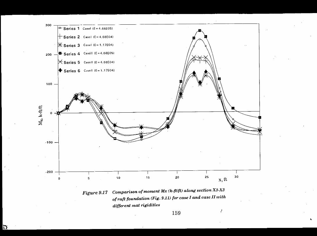
o

.100

.200

o 5 10 15 20 25 x, ft30

Figure 9.17 Comparison of moment Mx (k.(t/(t) along section X3-X3ofra(t foundation (Fig. 9.11) for case I and case II with

different mat rigidities

159 "~

400series 1 Casel IE =4.68E05)

Series 2 Casel IE = 4.68E04)

Series 3 Casel IE = 1.17E04)300 --l

Series 4 Casell IE = 4. 68E05)

Series 5 Casell IE = 4.68E04)

Series 6 Casell (E = 1.17E04)200

o

ct: 100

d:l~

f

.100

.200

0.0 5.0 10.0 15.0

y, ft20.0

Figure 9.18 Comparison of moment My (h.ff/ff) along section Y2.Y2ofraff foundation (Fig. 9.11) for case I and case II withdifferent mat rigidities

." 160,,'

.50

150series 1 Casel (E =4.68E05)

Series 2 Casel (E = 4.68E04)

Series 3 Casel IE = 1.1 7E04)

100 ~ Series 4 Casell (E = 4.68E05)

Series 5 Casell IE = 4. 68E04)

Series 6 Casell (E = 1.1 7E04)

I50

~~,~

i0

.100

0.0 5.0 10.0 15.0y, ft 20.0

Figure 9.19 Comparison of moment My (k-ftlft) along section Y4.Y4of raft foundation (Fig. 9.11) for case I and case II withdifferent mat rigidities

161

Chapter 10

CONCLUSIONS AND RECOMMENDATIONS

10.1 Conclusions

Thick plate analysis of footings and mat foundation were discussed inchapters 7, 8 and 9. From the findings of study the following conclusions canbe made :

a) Out of three Mindlin plate elements considered in the study, 4 nodedbilinear element fails to yield satisfactory results, while other twoelements e. g., 8 noded element and heterosis element are quite capable tomodel foundation problems. The vertical displacements, moments andshears obtained with this two elements are comparable.

b) The best order of quadrature is usually decided after numerical testing.For Mindlin plate elements it is found that reduced integration is theoptimum integration scheme. This requires 3x3 Gauss integration forbending and 2x2 Gauss integration for shear for both 8 noded element andheterosis element. For these two elements even a 2x2 Gauss integrationfor both bending and shear may be used without causing numericaldisaster.

c) Both 8 noded element and heterosis element are found quite efficient foranalysis of eccentric footing. For these elements the column moment canbe applied either as equivalent vertical loads or can be applied directly asmoments by distributing it at element nodes. When column moment isapplied as equivalent vertical load, the total equivalent vertical load P isdetermined by dividing the moment of particular direction by the columnwidth of that direction. This equivalent vertical load P is then applied atnodes on both faces of the column perpendicular to the direction of appliedmoment in opposite directions. In distribution of the load at nodes, eachcomer node should be given a load ofP/6 while each mid side node shouldbe given a load of 2P/3. When column moment is applied directly, it shouldbe distributed over 8 nodes with equal share i.e. each node should be givena moment value of MIS, where M is the column moment of particulardirection. However, the application of moment as equivalent vertical loadseems more realistic.

162

d) It is found that the behaviour of footings and mat foundation aresignificantly influenced by column fixity models. With improper columnfixity modelling, the actual behaviour of the foundation may not beproperly reflected. Fixed rotation column fixity model is found to be not.applicable for strip footings and mat foundations. For this type offoundation, fixity model which considers column loads to be uniformly.distributed over column area together with rotational stiffness of columnmay be used. However, column fixity model which includes above modelwith increased stiffness of column area is more close to reality.

e) It is found that the rotational stiffness of column computed as 4EIIL in thecolumn fixity models produces very little fixity and maximum momentsoccur at the centre of column areas. Since an unlimited effective depth offoundation mat is obtained across the column areas, column face momentsfor design is justifiable and the rotational stiffness of column may bealtogether neglected.

f) For column footing, moment values at the critical section considering fixedrotation at the column faces are found almost identical with those obtainedusing the fixity model corresponds to increased stiffness of column areatogether with the rotational stiffness of column. Therefore, for columnfooting, fixed column face rotation model may be used.

g) For footing supporting RC wall the moment at the critical section is foundalmost identical with ACI moment. For footing supporting masonry wallthe numerical value of the maximum moment is found to be close to themoment value using ACI method. However, using FE analysis themaximum moment is found to occur at the centre of the wall while the ACItheoretical maximum moment is based on assumed critical section at themid point of centre and face of the wall.

h) For square column footing, while the average moment at critical section isfound comparable with ACI moment value, the maximum value ofcomputed moment is found to be 210% of the ACI moment. This maximummoment occurs at the centre of column face and diminishes rapidlytowards the edges of the column. The moment value at a distance 6 inches

163.,.Ii'

outside the column edge is about 93% of ACI moment value, while at theedges of the footing it is found 53% of ACI values. This outward lowervalue of moments justify sloped footing construction.

/'i) Similar to spread footing, column face moments of mat foundation (and

strip footing) are found several times greater compared to the moments ofother portion of the mat. Therefore while the mat should he designed forthe average moments, additional reinforcements should be provided bothtop and bottom and to be extended upto a distance to satisfy developmentlength in column zone.

j) It is found that the rigidity of pile cap plays significant role for distributio:p.of 'applied load to individual piles. The conventional method fordetermination of pile loads using the combined stress equation is found tobe inadequate. The pile moments are found to have lower values usingrotational stiffuess of pile as 4EI/L.

k) The effect of soil zoning on deflections and moments of spread footing isfound very negligible. For mat foundation the effect becomes significantand is influenced by the mat rigidity. For relatively rigid mat, while thedisplacements obtained with soil zoning are comparable with thedisplacement obtained using single ks value, the positive momentsobtained with soil zoning become considerably higher surrounding interiorcolumn. This increase of positive moments is explained by beam action ofthe mat, caused by presence of soft springs under interior columns. Forrelatively flexible mat, beam action becomes less prominent and for bothcases moments obtained are comparable. The soil zoning (with softer soilnear the centre) seems more justifiable for situation when a rigid matrests on a strata of compressible soil extending to relatively greater depthor if there is a compressible layer under the.strata at a lower depth close tothe base of the mat. Because in such situations, though the base contactpressure may be considered nearly uniform, with increase of depth,greater compression would be produced in the soil under the centre of themat and this would tend to produce dish-shaped ground settlement. Butmat rigidity would oppose this dish-shaped ground settlement.'. ,Consequently, beam actlOn would occur and part of the central column

164 .,

loads will be transferred to the far edges. This would increase positivemoment surrounding the centre of the mat and high soil pressure beneath.the mat near the edges than the centre. As mentioned above in Winklerfoundation this effect can be achieved with soil zoning. For coarse grainedsoil the individual grains are somewhat mobile and the soil located to the

.perimeter can shift outward in the direction of lower soil stresses.The~efore, for coarse grained soil the above mentioned soil zoning may notbe justifiable. ,

1) In apparently uniform soil deposits, there are always lenses and pockets ofsoil having characteristics different from the typical or average. Whenweak pockets are located near the centre of a rigid mat, the positivemoment of the mat would increase significantly and interior column facemoment would be more critical. It is particularly important when weakpockets are located near the edges of a rigid mat. Since mats are normallyrigid this may cause to tilt the entire structure and soil zoning must beconsidered in such cases.

m) The variations of moments with the variation of footing rigidity is found tobe less sensitive for spread footing. For mat foundation moment variationsare found significantly sensitive with the mat rigidity. With the decreaseof mat rigidity significant pressure concentration occurs surrounding thecolumn and this lead to decrease both positive and negative moment of themat. This is also observed for mat foundation with soil zoning.

~ conventional method for analysis of mat foundation is found to beinadequate. With this method positive moment at the column face is foundvery small compared to the moment of FE analysis. The negative momentsobtained using approximate flexible method for most of the portion of themat are found significantly lower than the values of FE analysis. Thismethod fails to yield satisfactory results when the subsoil has very low ks

value compared to mat rigidity. Moreover this method is computationally.intensive and prone to calculation errors.

165

10.2 Recommendations

With necessary modification or addition, the present finite element programmay be used for other purposes. ,The application may be extended to linearand elasto-plastic analysis of plane stress, plain strain and axisymmetricproblems as well as elasto-plastic plate bending problems. However followingsuggestions are made for future development of the present research works.

a) In the present study the soil under the foundation mat is considered as aWinkler medium. For better representation of mat behaviour, the sub soilcan be modelledwith finite element of elastic continuum.

b) In the present study, the soil zoning considers doubled ks value near edgesthan that of centre of the mat and an average value in the intermediatezone. But soil zoning based on ks values for actual settlements of variouspoints under the mat would be more justifiable. In computing thesettlements, equations (Refs. 4 & 27) strictly applicable to flexible baseshould be used.

c) Since the concept of modulus of subgrade reaction is simpler and economiccompared to finite element of elastic continuum of subsoil, a comparativestudy can be made for the above cases to justify the applicability thesubgrade reaction concept.

d) Using the present finite element program rational design procedures forfootings and mat foundation can be developed and the inadequacy ofconventional method can be eliminated.

e) In the present study, 4 noded bilinear element fails to yield satisfactoryresults. But from economic point of view it is desirable to use lower orderelement. Although 8 noded element and heterosis eleme'nt used in thestudy are quite capable to model foundation problems and with theseelements the design shear can be obtained directly, a comparative studycan be made by using 4 noded thin plate element with displacementdescribed by polynomial of suitable degree to justify the applicability ofsuch element.

166

REFERENCES

1. ACI Committee 436 (at present Committee 336), Suggested DesignProceduces for Combined Footings and Mats, ACI J., Vol. 63, no. 10,Oct., 1966,pp 1041-1057.

2. Shukla, S.N., A Simplificel Method for Design of Mats on ElasticFoundation, ACI J., Vol. 81, no. 5, Sept.-Oct., 1984, pp 469-475.

3. Hossain, T.R., Comparative Study of the Anslysis Techniques of MatFoundation, M.Sc. Thesis, BUET, 1993, pp 112

4. . Bowles, J.E., Foundation Analysis and Design, 4th ed., Mc Graw-Hill, 1988, P. 998.

5. "Bowles, J. E., Analytical and Computer Method In FundationEngineering, Mc Graw - Hill, 1974, pp 209-254.

6. Borowicka, H., Influence of Rigidity df a Circular Foundation Slab onthe Distribution of Pressures Over a Contact Surface, 1st ICSMFE,Vol. 2,1936, pp 144-149.

7. Nilson, A.H. and Winter, G., Design of Concrete Structures, 9th ed.,McGraw-Hill Book Company, 1986, p. 725.

8. Richart, F. E., Rcinforced Wall and Column Footings, ACI J., Vol.45, Oct. -Nov., 1948,pp 94-127,pp 237-260.

9. Moe, J., Shearing Strength of Reinforced Slabs and Footings UnderConcentrated Loads, Portland Cement Association, Bull. no. D47,1961,p. 135.

10. Winkler, E., Die Lehre Vonder Elastizitat, und Festig Keit, Prag,1867,P.182.

11. Hetenyi, M., Beams on Elastic Foundations, the univ. of MichiganPress, 1946,p.255.

12. Teng, W.C., Foundation Design, Prentice-Hall, USA, 1962, p. 459.

13. Bowles, J.E., Foundation Analysis and Design, 2nd ed., MC-GrawHill Book Co.,NY, 1968, pp 294-320.

14. Owen, D.R.J. and Hinton, E., Finite Element in Plasticity, Pineridepress, Swansea U,K., 1980, pp 1-373.

167

15. Hughes, T.J.R and Cohen, M., The 'Heterosis' Finite Element for'Plate Bending, Computers and Structures 9, 1978, pp 445-450.

16. Rayapakse, R.K.N.D. and Selvadurai, A.P.S., A Comparative Studyon the Performance of Mindlin Plate Elements in Modelling Plate-Elastic Medium Interaction, Int. J. Nun. Meth. in Engrg., Vol. 23,1986,pp 1229-1244.

17. Cook, Robert D., Concepts and Applications of Finite ElementAnalysis, 2nd ed., John wiley & sons, New York, 1974, P. 537.

18. Road Research Laboratory, Soil Mechanics for Road Engineering,H.M's Stationery Office,London, 1952, pp 376-382.

19. Terzaghi, K., Evaluation of Co-officient of Subgrade Reaction,Geotcehnique, Vol. 5, no. 4, Dec., 1955, pp 297-326.

20. Vesic, A.S., Bending of Beams Resting on Isotropic Elastic Solid,Jour. Engrg. Mech. Divisiom, ASCE, Vol. 87, EM2, April, 1961, pp 35-53.

21. Vesic, A.S., Beams on Elestic Subgrade and the Winkler'sHypothesis, 5th ICSMFE, Vol. 1, 1961, pp 845-850.

22. Hinton, E. and Owen, D.R.J., Finite Element programmmg,Academic press, London, 1977, p. 303.

23. Irons, B. and Ahmed, S., Technique of Finite Elements, EllisHorwood Ltd., Sussex, U.K., p. 529.

24. Timoshenko, S., and Winowsky Krieger, S., Theory of Plates andShells, Mc Graw-Hill, 1959, p. 580.

25. Hinton, E., and Campbell, J.S., Local and Global Smoothing ofDiscontinuous Finite Element Function Using a Least SquareMethod, Int. J. Num. Meth, in Engrg. Vol. 8, 1974, pp 461-450.

26. Gorbunov- Pasadov, M. I and Screbrjanyi, R.V., Desgin of Structureon Elastic Foundation, Proc. 5th Int. Con£. Soil Mech. Fdn. Eng.,1961,pp 643-648.

27. Timoshenko, S., and Goodier, J.N., Theory of Elasticity, 2nd ed., McGraw - Hill Book Co., NY, 1951, pp 506.

168

Appendix ASample Input Data and Line Printer Output for

Slab and Foundation Problems

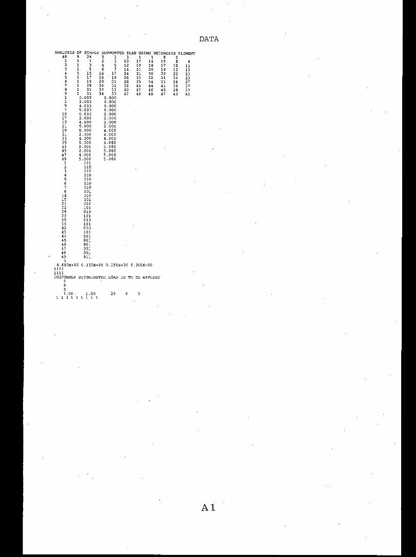
SUPPORTED SLAB USING HETEROSIS ELEMENT

Al

DATA

911132325

"333941

o,101222

"26363840

o15

"192931334345

"

1151820)0J2

"""48

1

"19213133J545

""

)101214

"2628384043

20

9 12 ), 56 ,16 1718 1920 2130 3132 3334 350.000O. 0000.0000.0002.-0002.0002.0002. 0004..0004..0004..0004..0005.0005.0005.0005.000

.001 1

OF SIMPLY

9 "1 11 )1 51 151 "1 191 291 311 330.0002.0004. .0005.000O. 0002.0004..0005.0000.0002. 0004.0005.000O. 0002. 0004.. 000S. 000111110110110110110110101010101010101010101010101010101001001001001001011

ANALYSIS4911J,56,,91)

5,15

"1921293133J54345

""11),56,,141521221829J5364343

"45""48491

4.680E .•05 0.150E .•00 O. 2S0E .•00 O. 900E .•0011111111UNIFOR.':lLY DISTRIBUTED LOAD IS TO BE APPLIED

ooo1. 00 .11111

OUTPUTANALYSIS OF SIMPLY SUPPORTED SLAB USING HETEROSIS ELEMENT

NPOIN= ., NELEM= NVFIX= 24 NNOOE.,

NMATS., NGAUS= NEVAB= " NALGO=

!RAFT., INTEP" NINCS=

ELEMENT PROPERTY NODE NUMBER1 1 1 2 3 10 17 16 15 8 92 1 3 4 5 12 " 18 17 10 113 1 5 6 7 14 21 20 19 12 134 1 15 16 17 24 31 30 29 22 235 1 17 18 19 26 33 32 31 24 256 1 19 20 21 28 35 34 33 26 277 1 29 30 31 38 45 44 43 36 ]78 1 31 32 33 40 47 46 45 38 399 1 33 34 35 42 ., 48 47 40 41

MAXIMUM FRONTWIOTH ENCOUNTERED" 39

A2

.000000000000000000000000000000000000000000000000000000000000000000000000000000000000000000

.000000000000

.000000000000

.000000

.000000

.000000

.000000

.000000

FIXED VALUES0.000000 0.0000000.0000000.0000000.0000000.0000000.0000000.0000000.0000000.0000000.000.000 0.0000000.0000000.0000000.000000 0.0000000.000000 0.00000'0o 000000 0.000000o 000000 0.000000o 000000 0.000000o 000000 0.000000o 000000 0.000000o 000000' 0.000000o 000000 0.000000o 000000 0.0000000.000000 0.0000000.0000000.0000000.000000 0.0000000.000000 0.0000000.000000 0.0000000.0000000.0000000.000000 0.000000

y

0.000o 000o 000o 000o 0000.0000.0001.0000.0001.0000.0001.0000.0001.0002.0002.0002.000,2.0002.0002.0002.0003.0000.000.3.0000.0003.0000.0003.0004.0004.0004.0004.0004.0004.0004.0004.5000.0004.5000.0004.5000.0004.5005.0005.0005.0005.0005.0005.0005.000

CODE111110110110110110110101

10101

10101

1010110

10110

10111111

11

,0.0001.0002.0003.0004.0004.5005.0000.0000.0002.0000.0004.0000.0005.0000.0001 0002 0003.0004 0004.5005 000o 000o 0002.000o 0004.0000.0005 000o 0001.0002.0003.0004.0004 5005 000o 0000.0002.0000.0004.0000.0005.0000.0001.0002.0003.0004.0004.5005.000

NODE123456789

1011121314151617181920212223242526272929303132333435363738394041424l444546474949

NODE12345678

1415212228293536474l444546474849

NUMBER ELEMENT PROPERTIES1 .46800E+06 15000E+00.25000E+00 90000E+00

COtNERGENCE PARAMETERIFDIS: 1 NCRES: 1110IFRES: 1 NCDIS: 1110

OUNIFORMLY DIS'!'RIBU'I'ED LOAD IS 'to BE APPLIEDooo

20MAX. NO, OF ITERATIONS:1.00000

A3

FINAL OU'I'PUT PARAMETER:

YZ-ROT .O.OOOOOOE--OOo 636655E-020.120418£-010.160252£-010.186436£-010.192973£-010.194474£-010.000000£ .•000.118650£-030,110223£-01o .169151E-030.173002E-Ol-0.398254E-040.181339E-OlO.OOOOOOE .•OOo ,474004E-020,894782£-02o ,120696E-Ol0.141150E-Ol0.146199£-010,147515£-010.000000£ .•00-0.208142E-040.619838E-020.215038E-040.984048E-02-0.103146E-050.103263£-010.000000£ .•000.168903£-020.313574E-020.433418E-020.502666E-020.519340E-020.525891E-020.000000£ .•00-0.270974E-04

CONVERGENCE TOLER£NC£

0.436£-03

0.186£-01

0.133E .•01

0.252E-02

o .188E"00

o .100E .•03

XZ-ROT.. OOOOOOE.•OO,OOOOOOE.•OO.000000£ .• 00.OOOOOOE.•OO

O.OOOOOOE.•OO0.000000£ .•00O.OOOOOOE+OO0.636653E-02o .118688E-03o .474002E-02-0.208177£-04o .168905E-02-0.2713191::-04O.OOOOOOE.•OO0.120419E-01o .110223E-Ol0.894782E-020.619842£-020.313577E-02o .160456E-02O.OOOOOOE.•OOo .160253E-Olo .169078E-030.120696E-010.214451E-040.433420E-02-0.360108£-040,000000£ .•000.186436E-Ol0.173002£-01o .141150E-010.984051E-020.502665£-020.253673£-020.000000£ .•000.192973£-01-0.398719E-04

PUT PARAMETER:

ITERATION NUMBER

ITERATION NUMBER 2

ITERATION NUMBER

DISPLACEMENTSNODE DISP,

1 O,OOOOOOE .•OO2 O. OOOOOOE.•OO3 O. OOOOOOE.•OO4 O. OOOOOOE.•OO5 o. OOOOOOE.•OO6 O. OOOOOOE.•OO7 O. OOOOOOE"OO8 0.000000£ .•009 O. OOOOOOE.•OO10 0.116721E-Ol11 0'.000000£ .•0012 0.181911£-0113 O.OOOOOOE .•OO14 0.190260E-0115 0.000000£ .•0015 0.116721E-Ol17 0.217353E-Ol18 0.293976£-0119 O. 340594E-Ol20 0.352774E-0121 0.356713E-Ol22 0.000000£ .•0023 O.OOOOOOE .•OO24 0.293976£-0125 O. OOOOOOE.•OO26 0,461517£-0127 0.000000;:: .•0028 O,483088E-0129 0, OOOOOOE.•OO30 0.181910E-0131 0.340593E-0132 0.461517E-013J 0.536049£-0134 0.555279£-0135 0.561570£-0136 0.000000£ .•0037 O.OOOOOOE .•OO

INCREMENT NUMBER 1LOAD FAC'tOR: 1.00000

INITIAL OU'I'-

0.193£-01 0.187E-Ol'tOTAL

-0.192E-01RESIDUAL NOR.'!

DISPLACEMENT CHANGE NORM

0.245E-03 .279E-03'tOTAL

-O,319E>03CONVERG<:NCE CODE

0.140E-01 .134£-02'tOTAL

-0.936E-02CONVERGENCE CODE

0.139E .•01 0.134E .•01'tOTAL

-0.138E .•01RESIDUAL NOR.J.~

DISPLACEMENT CHANGE NORM

0.100E .•03 0.100E .•03'tOTAL

-O,100E .•03RESIDUAL NORM

o . 114E .•Ol 148E .•00roTAe

-0.758E .•00CONVERGENCE CODE

DISPLAC&~ENT CHANGE NORM

IN CONVER

IN COWER

IN CONVER

38 0.352774£-01 0.1462008-01 0.1604518-0239 O.OOOOOOE+OO -0.976191£-06 -0.360108E-0440 0.555279£-01 0.519335E-02 0.253678£-0241 0.000000£+00 0.807586£-05 0.792404£-0542 o .581395E-01 0.000000£+00 0.263794£-024) O.OOOOOOE+OO o .19447)E-01 0.000000£+0044 0.190260E-01 0.181339£-01 0.000000£+00

" 0.356713E-01 0.147515£-01 0.000000£+0046 O.483088E-01 o .103252E-01 O.OOOOOOE+OO4) 0.561569£-01 O.525908E-02 0.000000£ •.004B 0.581394£-01 0.263794E-02 O.OOOOOOE+OO49 0.588100£-01 o .OOOOOOE+OO 0.000000£+00

REACTIONSNODE FORCE XZ-MOMEN'I' 'fZ-MOMENT

1 0 )06247£+00 -0.112528£+01 -0.112524E+01, -0 278050E+01 -0.439527£+01 0.000000£+003 -0 .376272£+00 -0.170488£+01 0.000000£+004 -0 .479919£+01 -0-,233249£+01 O.OOOOOOE+OO5 -0.389795E+00 -0.550393E+00 0.0000008+006 -0.2795298+01 -0.2308468+00 o .OOOOOOE+OO7 -0.2620248+00 -0.891789E-01 0.000000£+00B -0.278047£+01 0.000000£+00 -0.439517E+01

1< 0.000000£+00 -0.168376£+01 0.000000£+0015 -0.376262£+00 0.000000£+00 -0.170471E+0121 0.000000£+00 -0.156165E+01 O.OOOOOOE+OO22 -0.479943E+01 0.000000£+00 -0.233244E+012B 0.000000£+00 -0.4255698+01 O.OOOOOOE+OO29 -0.3898078+00 O.OOOOOOE+OO -0.5505308+0035 0.0000008+00 -0.1824808+01 O.OOOOOOE+OO36 -0.2794828+01 0.0000008+00 -0.2307218+0042 O.OOOOOOE+OO -0.245028E+01 O.OOOOOOE+OO43 -0.262382E+00 O.OOOOOOE+OO -0.891284E-01

" O.OOOOOOE+OO 0.0000008+00 -0.168367£+0145 0.000000£+00 O.OOOOOOE+OO -0.156153E+01

" O.OOOOOOE+OO 0.0000008+00 -0.425591E+0147 0.0000008+00 0.000000£+00 -0.182479£+0148 O.OOOOOOE+OO O.OOOOOOE+OO -0.245007£+0149 0.000000::+00 -0.666783E+00 -0.666890E+00

0 STRESSE~0 ELEMENT NO 1OG ,. X-COORD. 'i-COORD. X-MOMENT 'i-MOMENT X'i-MOMENT

1 0.2254 0.2254 0.17647E-01 0 17659£-01-0.34693£+012 0.2254 1.0000 0.15545E+00 0 13 92 5£+00-0.3 2114E+0 13 0.2254 1.7746 0.40107£+00 0 27702£+00 -0.28112£+014 1.0000 0.2254 o .13926E+00 0 1554 9E+00 -0 . 32114E+015 1.0000 1.0000 0.58303£+00 0 58303£+00 -0.292 03E+0 16 1.0000 1.7746 0.99707£+00 0 10061£+01-0 . 25454£+0 17 1.7746 0.2254 0.27703E+00 0 4010 9E+00 -0. 28112E"0 1B 1.7746 1.0000 0.10061£+01 0 99707 £+00 -0 . 25454£+019 1.7746 1.7746 o .15680E+01 0 156808+01-0 . 22 542E+0 1

OG ,. X-COORD. Y-COORD. Q-X Q-'1 0.4226 0.4226 0 .34920E+00 0 34904£+00, 0.4226 1.5773 0 .17426£+01 0 .10058E+013 1.5773 0.4226 0 .10060.:+01 0.17428£+014 1.5773 1.5773 0 .64954E+00 0.649528+00

0 ELENENT NO ,OG. ,. X-COORD. Y-CooRD. X-MOMENT Y-MOMENT XV-MOM£NT

1 2.2254 0.2254 27552E+00 .447228+00-0 .23812::+012 2.2254 1.0000 105048 .•.01 . 11671E .•.01-0 .225858 .•.013 2.2254 1.7746 174698 .•.01 .18753E .•.OI-0 .19899:: .•.01, 3.0000 0.2254 27778£ .•.00 .40358£+00-0 17660E .•.015 3.0000 1.0000 11359E .•.01 .13756£+01-0 16528E .•.Ol6 3.0000 1.7746 19399E+01 .23395E+01-0 14770E .•.017 3.7746 0.2254 30134E .•.00 .50197E+00-0 11363E .•.018 3.7746 1.0000 12134E .•.01 .15301E .•.01-0 10222E .•.019 3.7746 1.7746 20954E+01 .25538E .•.01-0 92890E .•.00

OG P. X-COORD. Y-CooRD. Q-X Q-Y1 2.4226 0.4226-0. 58821E+00 o. 21202E .•.012 2.4226 1.5773 0 11362E+01 0 .14809E+Ol3 3.5773 0.4226 0 .79855E+00 0 .24456E+014 3.5773 1.5773-0. 14967E+00 0 19036E+01

0 ELEXENT NO 3OG ,. X-COORD. 'i-COORD. X-MOMENT Y-MOMENT XY-MOME!'l"T

1 4.1127 0.2254 0 .34439£+00 0 578768+00-0 81781E .•.002 4.1127 1.0000 0 .12838E+01 0 15861£+01-0 73868E+003 4.1127 1.7746 0 .20696E+01 0 25703E .•.01-0 .66270E .•.004 '::.5000 0.2254 0 .33336E+00 0 58978E .•.00-0 44630E .•.005 4.5000 1.0000 0 .127168 .•.01 0 16159E .•.01-0 .43345E .•.006 4.5000 1.7746 0 .21193E .•.01 0 26284E .•.01-0 .38450E .•.007 4.8873 0.2254 0 31175E .•.00 0 .53028E .•.00-0 .82313E-01B 4.8873 1.0000 0 12559E+01 O. 16214E .•.01-0 .12240E+009 4.8873 1.7746 0 21722E .•.01 0 .27083E .•.OI-0 .870938-01

OG ,. X-COORD. Y-CooRD. Q-X Q-Y1 4.2113 0.4226-0 77918E+00 o .27808E .•.012 4.2113 1.5773 0 .83546E+00 0.12478E .•.Ol3 4.i8S7 0.4225 0 36710E .•.00 o .26664E+01, 4.7887 1.5773-0 .28816E .•.00 o .18585E+01

0 ELE.'-lENT NO. ,OG. ,. X-COORD. Y-CooRD. X-MOMENT Y-MOMENT X'l-MOMENT

1 0.2254 2.2254 0.447258+00 0 .27553 £.•.00 - 0 . 23812 £.•.012 0.2254 3.0000 o .40363E .•.00 0 27779E .•.00-0 .17660£+013 0.2254 3.7746 0.50197:: .•.00 0 . ]0135E .•.00-0 . 11362E .•.014 1.0000 2.2254 0.11671E .•.01 0 .10504E+ 01-0.22 584E .•.015 1.0000 3.0000 0.13756E+Ol 0 11360E+01-0 .16528E+016 1.0000 3.7746 0.15302:: .•.01 0 12134 E.•.01-0.1 02 22E .•.0 17 1.7746 2.2254 o .18752E .•.01 0 . 174 69E .•.01-0 .19899E+01B 1.7746 3.0000 0.23395E .•01 0 .19399:: .•.01-0.14769E+019 1.7746 3.7746 0.25538E .•.01 0 .2 0954E .•.0 1-0 .92887E+00

OG. ,. X-COORD. Y-CooRD. Q-' Q-'1 0.4226 2.4226 0 .21204E+OI-0 .58861E .•.002 0.4226 3.5773 0 .24454E+01 0 79884E+003 1.5773 2.4226 0 .14808E .•.01 0 11370E+01, 1.5773 3.5773 0 19034£ .•.01-0 15032:: .•.00

0 EL£)1ENT NO 5OG ,. X-COORD. 'i-COORD. X-MOMENT Y-MOMENT XY-MOMEl'."'1'

1 2.2254 2.2254 20590E .•.01 0.205908 .•.01-0.17056E+012 2.2254 3.0000 .24789E .•.01 o .22900E .•.01-0 .12952E+013 2.2254 3.7746 .28170E+01 o .25087E .•.01-0. 856308+004 3.0000 2.2254 .22900E+01 0.24789E+01-0.12952E+015 3.COOO 3.0000 .27728E+Ol O. 27728E+01-0. 964950: .•.006 3.0000 3.7746 .31490E+Ol Q. 30507E+ 01-0.61670£ .•.007 3.7746 2.2254 .25087£ .•.01 O. 28170E+01-0. 85632E+OO

A4

8 3.7746 J.OOOO )0507E+01 o . 31490£+01-0.616691> •.009 3.7746 3.7746 .34612£+01 a . 3 4612E .•01-0. 36967E .•OO

OC.P. X-COORD. ,(-COORD. Q-X Q-Y1 2.4226 2.4226 O.71362E .•00 O.71285E+00, 2.4226 :3.5773 o .87472E+00 O.7J146E+003 3.577) 2.4226 O.73085E+OO O.87514E+OO• 3.5773 . :3.577) 0.87875£+00 O.87854E:+00

0 ELEMENT NO 6OG ,. X-COORD. ,{-COORD. X-MOMENT ,{-MOMENT XY-MOMENT

1 It .1127 2.2254 0 .25004£+01 O. 29150E+0 1-0 . 610 11£+00, It .1127 3.0000 0 31431E+01 0.:3 2710E+0 1-0 .44682E .•003 4.1127 3.7746 0 35130£+01 0.35662£ .•01-0 . 26819E .•00• 4.5000 2.2254 0 254891>+01 0.297 66E+0 1-0 . 32265£+00., 4.5000 3.0000 0 31427£+01 0.))435£+01-0 . 25221£ .•0a6 1t.5000 3.7746 0 35472E+01 0.36821£ .•01-0.16540£+00, 4.8873 2.2254 0 25896£+01 0.29861£+01-0.55034£-018 4.8873 3.0000 0.313468+01 0.33 6528+0 1-0 . 597108-019 4.8873 3.7746 0.357<108+01 0.372 848 .•.0 1-0 . 4 6975E-0 1

OG. ,. X-COORD. V-COORD. Q-X Q-Y1 4.2113 2.4226-0.388078-010 .18865E+Ol2 4.2113 3 . 577 3-0.352148-01-0 .935728-02) 4.7887 2.4226 0.213928+00 0 .118718+01• 4.7887 3.57730.381598+000 .759168+00

0 8L8M8NT NO ,OG. ,. X-COORD. V-COORD. X-MOM8NT Y-MOM8NT XV-MOMENT

1 0.2254 4.1127 o .57872E+00 0 .3443 6E+00 -0 . 81783 8+00, 0.2254 4.5000 0.58977E+00 0 3333 5E .•.00 -0.44 629E+003 0.2254 4.8873 o .53023E+00 0 3117 6E+00 -0 . 82268E-0 1

• 1.0000 4.1127 0.158618+01 0 128378 .•.01-0.738708+005 1.0000 0:1.5000 o .16159E+Ol O. 12716E+0 1-0 .43 344E+006 1.0000 4.8873 0.162138+01 0 .12559E+OI-0 .12236E+00, 1.7746 4.1127 0.257048+01 0 20 696E+0 1-0 . 6627 58+008 1.7746 4.5000 0.25284::+01 0 . 21193E+0 1-0 . 384488+0 09 1.7746 4.8873 0.270838+01 0 .2172 2E+0 1- 0 .87021E-01

OG. ,. X-COORD. V-COORD. Q-X Q-Y1 0.4226 4.2113 0 27810E+01 0 .77921E+002 0.4226 4.7887 0 26653E+01 0 .36661E+003 1.5773 4.2113 0 .124828+01 0 .83604E+00• 1.5773 4.7887 0 18584E+01 0 .28805E+00

0 ELSMENT.NO. 8OG ,. X-COORD. V-COORD. X-MOMENT V-MOMENT XV-MOM::NT

1 2.2254 4.1127 29149E+01 .25004E+01-0 .61018E:+00, 2.2254 4.5000 29766E .•.01 .25489E+OI-0 .322658+003 2.2254 4.8873 .298628+01 .25895E+OI-0. 54937E-01, 3.0000 4.1127 0.327108+01 0.31431E .•.OI-0 .44682E+00, 3,0000 4.5000 0.33436E+01 0.314278+01-0 .25219E+006 3.0000 4.8873 0.336518+01 0.31)46E+01-0. 59651E-01, 3.7746 4.1127 0.358628+01 0.35129E .•.OI-0 .26816E+008 3.7746 4.5000 0.36821::+01 o .35472E+OI-0. 16544E+009 3.7746 4.8873 0.37282E+01 0.35741E+OI-0 .470698-01

OG ,. X-COORD. V-COORD. Q-X Q-Y1 2.4226 4.2113 0 188718+01-0 .393618-01, 2.4226 4.7887 0 118688+01 0 .21354E+003 3.5773 4.2113 0 93602E-02-0 .35562E-Ol• 3.5773 4.7887 0 .75912E+00 0 .38295E+00

0 ELEMENT NO. ,OG. ,. X-COORD. V-COORD. X-MOMENT V-MOMENT XY-MOMENT

1 4.1127 4.1127 .35815E+01 0 .3581 5E+0 1-0.1849 9E+00, 4.1127 4.5000 .36656E+Ol 0 . 36412E+0 1-0 .10714E+003 4.1127 4.8873 .37306E+Ol 0 .3 6981E+0 1-0.2625 5E-01

• 4.5000 4.1127 .364138+01 0 .3 6658E+0 1-0 .10718E+005 4.5000 4.5000 .37232E+Ol 0 37232E+O 1-0.536178-016 4.5000 <1.8873 .37673E+Ol 0 3770:19E+0 1-0.4810 3E-02, 4.8873 4.1127 .36981E+Ol 0.373058+01-0.262158-018 4.8873 4.5000 .377518 .•.01 0.3767 3E+01-0. 487218-029 4.8873 4.8873 .37956E+Ol 0.37956E .•.01 0.393948-02

OG. ,. X-COORD. V-COORD. Q-X Q-Y1 4.2113 4.2113 0 132558 .•.01 0 132708+012 4.2113 4.7887 0 .67987E-OI-0 67620E .•.00) 4.7887 4.2113 0 .67345E+00 0 67321E-01

• 4.7887 4.7887 0 .32795E .•.00 0 32881E+001 1 1 1 1 1 1 1 1

ONODE NO X-COORD V-COORD X-MOMENT Y-MOMENT XV-MO~NT1 0.0000 0.0000 -0 35763E-05 -0.28014E-05 -0.355678 .•.012 1.0000 0.0000 0 45356E-02 0.30238E-Ol -0.328038+013 2.0000 0.0000 0 460098-01 0.30677E+00 -0.26505E+01

• 3.0000 0.0000 0 178818-01 o . 11920E .•.00 -0.17872E+015 4.0000 0.0000 0 39505E-01 0.26339E+00 -0.97597E .•.006 4..5000 0.0000 0 43301E-01 0.28864E .•.00 -0.443258+00, 5.0000 0.0000 0 26093E-01 o .17391E+00 0.53916E-018 0.0000 1.0000 0 30188E-Ol 0.45262E-02 -0.328038+019 0.0000 0.0000 0 .583038+00 0.58303E+00 -0.292038+01

10 2.0000 1.0000 0 10762E+Ol o .11041E+01 -0.24253£+0111 0.0000 0.0000 O. 11359E+Ol o . 13756E .•.01 -0.16528E .•.0112 4.0000 1.0000 0 .126058+01 0.15689E+01 -0.83021£+0013 0.0000 0.0000 0 .12716E+Ol o .16159E+01 -0.43345<:+0014 5.0000 1.0000 0 . 12506E .•.Ol o .16184E+01 -0.30783E-0115 0.0000 2.0000 0 .30677E+00 o .46013E-01 -0.26505£+0116 1.0000 2.0000 0 .110418+01 o .10762E .•.01 -0.24253E+0111 2.0000 2.0000 0 .18620E+Ol o . 18621E.,.01 -0.20140E+0118 3.0000 2.0000 0 .21465E+Ol 0.25044E+01 -0.14010E .•.0119 4.0000 2.0000 0 .23143E+Ol o .28184E+01 -0.75078E+0020 4.5000 2.0000 0 23447E+Ol 0.28925E .•.Ol -0.35177E+00n 5.0000 2.0000 0 .24447E+Ol 0.296298+01 0.29205E-Ol22 0.0000 3.0000 0.11925E+00 0.17885E-Ol -0.17872E+Ol23 0.0000 0.0000 0.13756£+01 0.11360E+01 -0.16528E+Ol24. 2.0000 3.0000 0.25044E+01 0.21465E+Ol -0.14010E+Ol

" 0.0000 0.0000 0.27728£+01 0.27728E+Ol -0.96495E+00

" 4.0000 3.0000 0.31352E+Ol 0.323942+01 -0.50790E+00

" 0.0000 0.0000 o .31427E+Ol 0.33435E+01 -0.25221E+0028 5.0000 3.0000 0.31309£+01 0.33619£+01 -0.40901E-02

" 0.0000 4.0000 o .26334E"'00 o .39494E-01 -0.97596£+0030 1.0000 4.0000 0.15689£+01 o .12605E+01 -0.83023£+0031 2.0000 4.0000 0.28184E+01 o .23144E+Ol -0.75080£+0032 3.0000 4.0000 0.32394E .•.01 0.31351E+Ol -0.50792E+0033 4.0000 4.0000 0.35905E .•.01 0.35904E .•.Ol -0.23158E+0034 4.5000 4.0000 0.361998+01 0.37116E+Ol -0.13036E+0035 5.0000 4.0000 0.36882E+01 0.37870E+Ol -0.786478-0236 0.0000 4.5000 0.28862£+00 0.43291E-Ol -0.44324E+00

" 0.0000 0.0000 0.161592+01 0.12716E+Ol -0.43344£ .•.0038 2.0000 4.5000 o .28925E+Ol 0.23447E+Ol -0.35176E+0019 0.0000 0.0000 0.33436E+Ol 0.314278+01 -0.25219E+00

A5

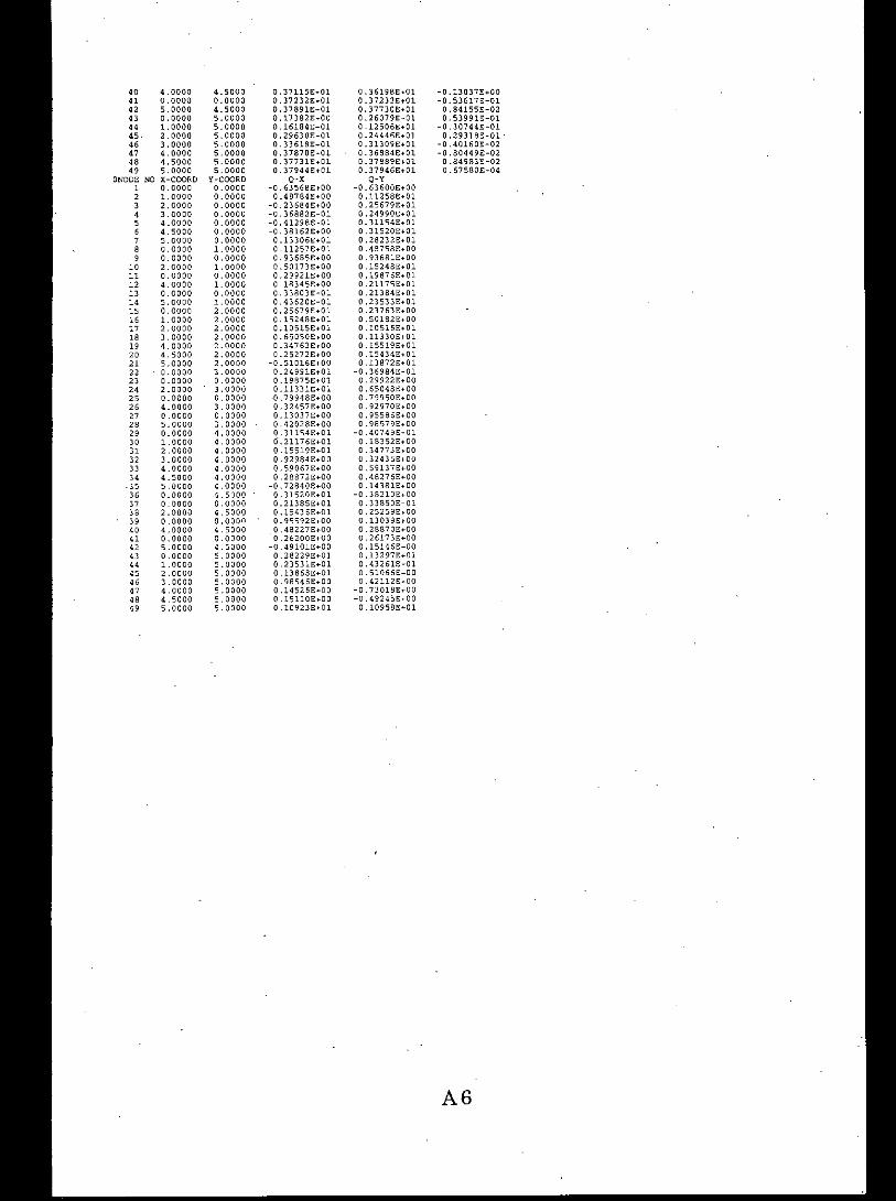
40 4.0000 4.5000 0.371150: .•01 0.361988+01 -0 13037E+00<l 0.0000 0.0000 0.372328+01 0.37232E+01 -0 53617E-0142 5.0000 4.5000 0.37891E+01 0.37730E+01 0 84155E-0243 0.0000 5.0000 o .17382E+00 0,260798-01 0 53991E-01

" 1.0000 5. 0000 a .16184E+01 0.12506E+01 -0.30744E-0145. :2.0000 S. 0000 0.296308+01 0.244468+01 0.29318E-Ol-46 3.0000 5.0000 0.33618E+01 0.313098+01 -0.40160E-0247 4..0000 5.0000 0.378708+01 O.36884E+01 -0.80449E-0248 4.5000 5. 0000 0.]7731E+01 0.378891::+01 o .84983E-02" 5.0000 5.0000 0.)79448+01 O.37946E+01 O.67580E-04

ONODE NO X-COORD Y-COORD Q-X Q-Y1 0.0000 0.0000 -0 .63568£+00 -0.63600E+00, 1.0000 0.0000 0 .487848+00 0.112588+013 2.0000 0.0000 -0 .23684E+00 O.25679E+01• 3.0000 0.0000 -0 .36882E-01 0.249908 .•015 4.0000 0.0000 -0 .412988-01 0.311548 .•016 4.5000 0.0000 -0 381528 .•00 o .31520E .•017 5.0000 0.0000 0 133058 .•.01 0.282328 .•018 0.0000 1.0000 0 .112578 .•01 0.487588 .•009 0.0000 0.0000 0 .935858 .•00 0.935818 .•0010 2.0000 1.0000 0 50173E .•00 0.152488 .•0111 0.0000 0.0000 0 .299218 .•00 a .19875E .•Ol12 4.0000 1.0000 0 .18345E .•00 0.211758 .•0113 0.0000 O. 0000 0 .33803E-01 0.213848 .•011. 5.0000 1. 0000 0.43520E-01 0.23533E .•0115 0.0000 2. 0000 o .25579E .•01 -0.23753E .•0016 1.0000 2. 0000 o . 15248E .•01 o .50192E .•0017 2.0000 2.0000 o .10515E .•01 o .10515E .•0118 3.0000 2.0000 0.65050E .•00 o . 11330E .•Ol19 4.0000 2.0000 0.34763E .•00 o . 15519E .•0120 4.5000 2.0000 0.25272E .•00 0.154348 .•0121 5.0000 2.0000 -0.510158 .•00 0.138728 .•01

" 0.0000 3.0000 0.249HE .•01 -0.359848-0123 0.0000 0.0000 0.198758 .•01 0.29922E .•0024 2.0000 3.0000 0.11331E .•01 0.550481': .•0025 0.0000 0.0000 0.79948E .•00 0.79950E .•0026 4.0000 3.0000 0.32457E .•00 0.929708 .•0027 0.0000 O. 0000 0.13037E .•00 0.95586E .•0028 5.0000 3.0000 0.42028E .•00 0.985798 .•0029 0.0000 4.0000 0.311548 .•01 -0.40749E-Ol30 1.0000 4.0000 0.211768 .•01 o .18352E .•0031 2.0000 4.0000 0.15519E .•01 0.34773E .•00J2 3.0000 4.0000 0.929848 .•00 0.32435E .•0033 4.0000 4.0000 0.590678 .•00 0.59137E .•0034 4..5000 4.0000 0.288728 .•00 o .48276E .•00.J5 5. 0000 4.0000 -0.72840E .•00 0.143818 .•0036 O. 0000 4.5000 0.31520E .•01 -0.38210E .•00J7 0.0000 0.0000 0.21385E .•01 0.33850E-01J8 2.0000 4.5000 0.15436E .•01 o .25259E .•0039 0.0000 0.0000 0.95592E .•00 o .13039E .•00'0 4.0000 4.5000 0.48227E .•00 o .28870E .•00., 0.0000 0.0000 0.26200E .•00 0.26173E .•0042 5.0000 4.5000 -0.49101E .•00 0.15146E .•004J 0.0000 5.0000 0.28229E .•01 0.13297E .•0144 1.0000 5.0000 o .23531E .•01 o .43261E-0145 2. 0000 5.0000 o .13868E .•01 -0.51066E .•00.6 3.0000 5.0000 o .98545E .•00 0.42112E .•OO47 4.0000 5.0000 0.14526E .•00 -0.73018E .•0048 4.5000 5.0000 0.15110E .•00 -0.49245E+0049 5.0000 5.0000 o .10923E+01 o .10958E+01

A6

100. 000100. 000100. 000100. 000100. 000100. 000100. 000100.000100. 000100. 000100.000100 .000100. 000100. 000100. 000100. 000100. 000100. 000100.000

1.0011111

1.00 201111111

1111111110

AS

OUTPUTANALYSIS OF SPREAD FOOTING

N?OIN~ 96 NELEM" 25 NVF!X" 24 NNODE=

NMATS" NGAUS= NE:VA8" 24 NALGO=

lRAFT= INTEP= NINeS"

ELEMENT PROPERTY NODE NUMBER1 1 1 , 3 13 20 19 18 12, 1 3 4 5 14 " 21 20 133 1 5 5 7 15 24 " " 144 1 7 , 9 15 25 25 24 155 1 9 10 11 17 28 " 25 155 1 18 19 20 30 37 35 35 297 1 20 21 " 31 39 3B 37 308 1 " " 24 32 41 40 39 319 1 24 25 25 33 43 42 41 3210 1 25 " 28 34 45 44 43 3311 1 35 35 37 47 54 53 53 4512 1 37 3B 39 48 96 55 54 4713 1 39 40 41 49 58 " 96 4814 1 41 42 43 50 60 59 58 4915 1 4l 44 45 51 52 51 50 5015 1 53 53 54 " 71 70 59 5317 1 54 55 96 55 33 72 71 "18 1 96 " 58 " 75 74 33 5519 1 58 59 60 " " " 75 "20 1 60 51 52 " 79 78 " "21 1 69 70 71 81 88 87 86 80

" 1 71 72 33 " 90 89 88 81

" 1 33 74 75 83 92~ 91 90 8224 1 75 " " 84 94 93 92 8325 2 " 78 79 85 96 95 94 84

NODE , Y1 . 000 0 000, 500 0 0003 1. 000 0 0004 1. 500 0 . 0005 2. 000 0 . 0005 2.500 0 . 0007 3. 000 0 . 0008 3.500 0 . 0009 4. 000 0 ,00010 4.500 0 00011 S. 000 0 .00012 O. 000 0 .50013 -1.000 0 .50014 :2.000 0 .50015 ). 000 0.50015 4.000 o. sao17 5. 000 0.50018 O. 000 1. 00019 0.500 1. 00020 1. 000 1. 00021 1. 500 1. 000

" 2. 000 1. 000

" 2.500 1. 00024 3.000 1. 00025 3.500 1. 00025 4. 000 1. 000

" 4. sao 1. 00028 5. 000 1.00029 0", 000 1. 50030 i.. 000 1.50031 2. 000 1.50032 3. 000 1.50033 4. 000 1.50034 5. 000 1.50035 O. 000 2. 00035 0.500 2.00037 1.000 2.0003B 1.500 :2. 00039 2.000 2.00040 2.500 2.00041 ) .000 2.00042 3.500 2.00043 4.000 2.00044 4.500 2.00045 5. 000 2. 00045 0.000 2. sao47 1.000 2.5004B 2.000 2.50049 3.000 2.50050 4. 000 2.50051 5. 000 2.50052 O. 000 3. 00053. o. sao 3. 00054 1. 000 L 00"055 1. sao 3. 000

" 2.000 LOOO

" 2.500 3. 00058 3. 000 3. 00059 3.500 3. 00060 4. 000 3. 00051 4. sao 3.000

" 5. 000 3. 00063 O. 000 3. sao

" 1. 000 3. sao55 2. 000 3.50066 3. 000 3. sao67 4. 000 3.50068 5. 000 3.50069 O. 000 4. 00070 O. sao 4.00071 000 4. 00072 500 4. 000

'" A9

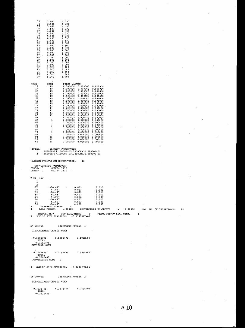
MAXIMUM FRONTWIDTH ENCOUNTERED~ 48

INITIAL OUT PUT PARAMETER= 0SUM OF SOIL REACTION~ -0.119901£ .•03

20MAX. NO. OF ITER. •••TIONS"1.00000

AlO

.000

. 000

.000

.000

.000

.000000000

FINAL OUTPUT PAR.'\METER~

0.0000000.000000O. 000000o. 000000o. 000000O. 000000o. 000000o. 0000000.000000O. 0000000.0000000.0000000.0000000.0000000.0000000.0000000.000000O. 000000o. 0000000.000000O. 000000O. 000000o. 0000000.000000

0.249E .•Ol

0.369E •.00

o .100E •.03

a 000a 000a 000a 000a 000O. 0000.000O. 000

CONVERGENCE TOLERENCE

~0.124795E .•03

4. 0004.0004.0004.0004. 0004. 0004. 0004 5004.5004 sao4 5004 5004.5005. 0005. 0005.0005. 0005.0005.0005.0005.0005.0005.0005.000

FIXED VALUES.000000 0.000000.000000 0.000000. 000000 0.000000. 000000 0.000000.0000000.000000.000000 0.000000.000000 0.000000. 000000 0.000000.0000000.000000.000000 0.000000.000000 0.000000.000000 0.000000.000000 0.000000000000 0.000000000000 0.000000000000 0.000000

0.000000 0.0000000.000000 0.0000000.000000 0.0000000.000000 0.0000000.0000000.0000000.000000 0.0000000.0000000.0000000:000000 0.000000

ITERATION NUMBER 2

ITERATION NUMBER

0.252E .•Ol

CODE1010101010101010111111111111111111111111

2.0002.5003.0003.5004.0004.5005.0000.0001.0002. 0003. 0004. 0005. 000o. 0000.5001. 0001.5002. 0002.5003. 0003.5004. 0004.500'5. 000

ELEMENT PROPERTIES.4 6800E .• 0 6. 15000E .•0 0.2 0000E .•01 OOOOOE.•0 0.4 6800E .•07 .15000E .•00 . 2 0000E .•01 OOOOOE.•Oa

0.392E .•OlTOTAL

-0.392E •.Ol

KS 1001o277 -10.41778 41.66779 -10.41784 41.66785 41.66794 -10.41795 41.66796 -10.417

INCREMENT NUMBER 1LOAD FACTOR" 1.00000

DISPLACEMEN7 CHANGE NOflM

a .100E .•0) a .100E"0)TOTAL

-0.100E .•03RESIDUAL NORM

0.174£ .•01 .215E •.00TOTAL

-0.998E •.00CONVERGENCE CODE

SUM OF SOIL REACTION"

DISPLACEMENT CHANGE NORM

NODE111728344551

"6877787984as8687888990919293949596

73

"75767778798081828384858687888990919293949596

NUMBER1,

IN CONIfER

CONVERGENCE PAR&~ETERIFDIS= 1 NCRES" 1110IFRES" 1 NCDIS" 1110

IN COtNER

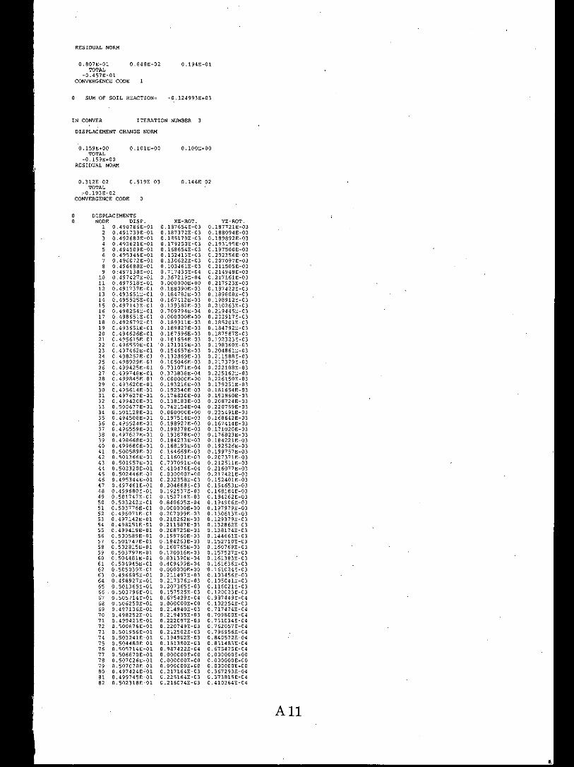
IT8RATION NUMBER 3

XZ-ROT.0.1876548-030.1873728-030.1851798-030.1792508-030.1686548-030.1524138-030.1306228-030.1034618-030.717435E-04o 3672198-04o 0000008+000.1880908-030.1847828-030.1674128-030.129382E-030.7097948-040.000000£+000.189911£-030.1898278-030.187596£-030.1816548-03'0.171019£-030.1546578-030.1328698-030.1050468-030.7310718-040.373838£-04o 0000008+00o 193216£-030.1923408-03o 176830E-03o 1381838-03o 762154£-040.0000008+00o .197514E-03o .198927E-030.198378£-030.1938788-030.1842338-030.1681938-03o .144669E-030.1160318-030.7970918-040.4104768-040.0000008+000.202358£-030.2048688-030.1925378-03o .152714E-030.8406058-040.000000£+00o .207099E-030.210262£-030.2115878-030.2087258-030.1997608-030.1842638-030.1607658-030.1200168-030.8313908-040.4094998-040.0000008+000.2114978-030.217376£-030.2073658-030.1575258-030.6754298-040.0000008+000.2149408-030.2194358-030.2220978-030.2207498-030.2125028-030.1949028-030.1613808-030.9874228-040.0000008+000.0000008+000.0000008+000.2171648-030.2251648-030.2160748-03

•

All

YZ-ROT.1877218-03

0.1880948-03o .189892E-030.1931958-030.1975008-030.2023568-030.207097E-030.2115058-030.2149488-030.2171618-030.217923£-030.1874228-030.1898088-030.1989128-030.2102638-030.2194458-030.2229178-030.1852018-030.1847928-030.1875878-030.1923238-030.1983608-030.2048618-030.2115888-030.2173798-030.222108E-030.2251628-03o .226150E-03o .179251E-030.1816541;:-030.1938608-030.2087248-030.2207598-030.2254918-030.1686421;:-030.1674148-030.1710208-030.1768238-030.1842218-030.1925268-030.1997578-030.2073718-030.2125118-030.2160778-030.2114218-030.1524018-030.1546538-030.168184£-030.184262£-030.1949068-030.1979798-030.1306138-030.1293798-030.1328628-030.1381748-030.1446618-030.1527108-030.1607698-030.1575278-030.1613838-030.1616368-030.1610248-030.1034568-030.1050418-030.1160218-030.1200238-030.9814498-040.1022548-030.7174748-040.7098008-040.7310348-040.762057£-040.796956E-040.8405728-040.8314838-040.675475£-040.0000008+00O.OOOOOOE+OO0.0000008+000.367293E-040.373815E-040.410364£-04

0.1008+00

0.1468-02

0.1948-01

-0.1249938+03

DISPLACEMENTSNODE DISP.1 0.490786E-012 0.491739E-013 0.492680E-014 0.4936218-015 0.494509E-Ol6 0.4953468-017 0.496072E-Ol8 0.496688£-019 0:497138£-0110 0.497427£-0111 0.4975188-0112 0.491737E-0113 0.493651E-Ol14 0.4955258-0115 0.497143E-Ol16 0.4.982548-0117 0.498651E-0118 0.492679E-Ol19 0.4936518-0120 0.494626E-Ol21 0.495615E-Ol22 0.4965598-0123 0.4974628-0124 0.498252E-0125 0.498929E-Ol26 0.4994258-0127 0.4997488-0128 0.499845£-0129 0.4936208-0130 0.4956148-0131 0.4976278-0132 0.4994208-0133 0.5006778-0134 0.5011288-0135 0.4945088-0136 0.4955248-0137 0.4965598-0138 0.497627E-Ol39 0.4986688-0140 0.4996808-0141 0.5005898-0142 0.5013668-0143 0.501957E-Ol44 0.5023208-0145 0.5024468-0146 0.4953448-0147 0.4974618-0148 0.4996808-0149 0.5017478-0150 0.5032428-0151 0.5037768-0152 0.4960718-0153 0.4971428-0154 0.4982518-0155 0.499419£-0156 0.5005898-0157 0.5017478-0158 0.5028158-0159 0.503797E-Ol60 0.5044818-0161 0.5049458-0162 0.505039E-0163 0.4966858-0164 0.4989278-0165 0.5013658-0166 0.5037968-0167 0.5057148-0168 0.5062508-0169 0.4971368-0170 0.4982528-0171 0.4994238-0172 0.5006768-0173 0.501956E-0174 0.503241£-0175 0.504480E-0176 0.5057148-0177 0.506870E-0178 0.507026E-0179 0.507070E-0180 0.4974248~0181 0.499745E-0182 0.5023188-01

SUM OF SOIL REACTION~

0.807E-Ol .8488-02TOTAL

-0.4578-01CONVERGENCECODE

0.159E+00 0.101E+00TOTAL

-0.159E+00RESIDUAL NORM

DISPLACEMENT CHANG8 NORM

RESIDUAL NORM

0.312E-02 .519E-03TOTAL

.-0.193E-02CONVERGENCECODE

IN CONVER

83 0.5049448-01 0.1616281'>03 0.4095718-04

" O.507025E~Ol 0.0000008 .•00 0.000000£+0085 0.5071138-01 0.000000£ •.00 0.0000008 .•0086 0.4975148-01 0.211933£-03 0.0000008+0087 0.496648£-01 0.2229308-03 O.OOOOOOE .••OO88 0.4996428-01 0.226163£-0) 0.000000£ •.0089 O,501126E-01 O.225497E-0) 0.0000008+0090 o .502444E-Ol O.217415E-OJ 0.0000008 .•.0091 O.503774E-01 0.1979558-03 o .OOOOOOE .•.OO

" 0.505037E-Ol a .161013E-03 0.0000008 •.0093 0.506249£-01 0,1022538-03 0.000000£ .•0094 0.507070E-01 0.000000£+00 0.0000008+0095 0.5071138-01 0,0000008 .•00 O.OOOOOOE+OO95 0.5071598-01 0.0000008 .•.00 0.0000008+00

1 1 1 1 1 1 1 1 1 1 1 1 1 1 1 1 1 1 1 1 1 1 1 1 0ONODE NO X-COORD Y-CooRD X-MOMENT "{-MOMEN'!' XY-MOMENT1 0.0000 0.0000 -0.49320E+00 -0.487058 .•00 0.161618+00, 0.5000 0.0000 0.75395£ .•.00 -0.12264£ .•.00 -0.40551£-023 1.0000 0.0000 0.20580£ .•.01 -0.30546£ .•.00 -0.17795£ .•.004 1.5000 0.0000 0.51200£ .•.01 -0.23903£+00 -0.26472£ .•.005 2.0000 0.0000 0.81953£ .•.01 -0.26480£ .•.00 -0.32397E .•.006 2.5000 0.0000 0.11837£ .•.02 -0.19271£ .•.00 -0.30729£ .•.007 3.0000 0.0000 0.15392£ .•.02 -0.24067£ .•.00 -0.32122£ .•.008 3.5000 0.0000 0.18336£ .•.02 -0.22872£ .•.00 -0.24648£ .•.009 4.0000 0.0000 0.21239£ .•.02 -0.19271£ .•.00 -0.20089£ .•.00

10 4.5000 0.0000 0.22344£ .•.02 -0.26624£ .•.00 -0.10110£ .•.0011 5.0000 0.0000 0.23422£ .•.02 -0.153l4.£+00 +0.10240E-0112 0.0000 0.500"0 -0.11828£ .•.00 0.76875E .•.OO -0.17391£-0213 1.0000 0.5000 0.25643E .•.01 0.11037£ .•.01 -0.12650£ .•.0114 2.0000 0.5000 0.85418£ .•.01 o .10128E .•.01 -0.18569£ .•.0115 3.0000 0.5000 o . 15542E .•.02 0.93033E .•.00 -0.18425£ .•.0116 4.0000 0.5000 0.21153£ .•.02 0.93921E .•.00 -0. 11443E .•.0117 5.0000 0.5000 0.23334E .•.02 0.93333E .•.00 O. 57543E~0218 0.0000 1.0000 ~O. 30605E .•.00 0.20761£ .•.01 -0.17672£ .•.0019 0.5000 1.0000 0.11071£ .•.01 0.25646E .•.01 -0.12640E .•.0120 1.0000 1.0000 0.25313E .•.01 0.25230£ .•.01 -0.23058£ .•.0121 1.5000 1.0000 0.55454£ .•.01 0.24900E .•.01 -0.28044E .•.01

" 2.0000 1.0000 0.86651E .•.01 0.23802£ .•.01 -0.32721£ .•.01

" 2.5000 1.0000 0.12234£ .•.02 0.22077£ .•.01 -0.33266E .•.0124 3. 0000 1.0000 0.16015£ .•.02 0.22170£ .•.01 -0.32206E;'0125 3.5000 1.0000 o . 18950E .•.02 0.20318£ .•01 -0.26908£ .•.0126 4.0000 1.0000 0.21804E .•.02 0.20700£ .•.01 -0.20040£ .•.0127 4.5000 1.0000 0.23104E .•.02 o . 19629E .•.01 -0.10118E .•.0128 5.0000 1. 0000 0.24136E .•.02 o .19364E .•.01 o .12140E-0129 0.0000 1.5000 -0.23866E .•.00 0.51303E .•.01 -0.26705E .•.0030 1.0000 1.5000 0.24941E .•.01 0.55432E .•.01 -0.28023E .•.0131 2.0000 1.5000 0.88293E .•.01 0.57360E .•.01 -0.38825E .•.0132 3.0000 1.5000 o .16800E .•.02 0.62114E .•.01 -0.36075E .•.0133 4.0000 1.5000 0.23750E .•.02 0.65567E .•.01 -0.20837E .•.0134 5.0000 1.5000 0.26036E .•.02 0.66289E .•.01 -0.60245E-0135 0.0000 2.0000 ~0.26403E .•.00 o .81988E .•.01 -0.32583E .•.0036 0.5000 2.0000 0.10123E .•.01 o .85450E .•.01 -0.18552E .•.0137 1.0000 2.0000 o .23788E",01 0.866811': .•.01 -0.32679£ .•.0138 1.5000 2.0000 0.57375E .•.01 0.882902 .•.01 ~O.38806E .•.0139 2.0000 2.0000 0.89978E .•.01 0.89945E .•.01 -0.46231E .•.0140 2.5000 2.0000 0.13775£ .•.02 0.95402E .•.01 -0.43759E .•.0141 3.0000 2.0000 0.17743E .•.02 o .99978E .•.01 -0.41589E .•.0142 3.5000 2.0000 0.21906E .•.02 o .10920E .•.02 -0.32083E .•.0143 4.0000 2.0000 0.25800E .•.02 o .10529E .•.02 -0.26120E .•.0144 4.5000 2.0000 0.26505E .•.02 o .10902E .•.02 -0.12917E .•.0145 5. 0000 2.0000 0.28041E .•.02 0.11213E .•.02 -0.62919E-0146 0.0000 2.5000 -0.19336E .•.00 o .11836E+02 -0.30997£ .•.0047 1.0000 2.5000 0.22057E .•.01 o . 12236E .•.02 -0.33223E .•.0148 2.0000 2.5000 0.95413E .•.01 o . 13774E .•.02 -0.43744E .•.0149 3.0000 2.5000 0.21041E .•.02 a .15320E .•02 ~0.36101E .•0150 4.0000 2.5000 o .27245E+02 0.20038E .•.02 -0.19188E .•.0151 5.0000 2.5000 0.29897E .•02 0.22080E .•.02 o .20527E-0252 0.0000 3. 0000 -0.24001E .•.00 o . 15390E .•02 -0.32312E .•.005) 0.5000 3.0000 o .93108E"'00 o .15543E .•02 -0. 18420E .•.0154 1.0000 3.0000 o .22165E .•01 o . 16015E .•.02 -0.32181E .•.0155 1.5000 3.0000 0.62102E .•.01 o .16801E .•.02 -0.36054E .•.0156 2.0000 3.0000 0.99977£ .•.01 0.17743E .•.02 -0.41566E .•0157 2.5000 3.0000 o .15322E .•.02 0.21040E .•02 ~O. 36099E .•.0158 3.0000 3. 0000 0.25761E .•.02 0.25158£ .•.02 -0.34438E .•.0059 3.5000 3.0000 0.219251:: .•.02 0.24703E .•.02 -0.15956£ .•.0160 4.0000 3.0000 0.28936E .•.02 0.31193E .•02 -0.20226E .•.0151 4.5000 3.0000 o .30604E .•.02 o .31098E .•.02 -0.33285E .•.0062 5.0000 3.0000 o .29707E .•.02 0.30271£ .•.02 o .28384E .•.0063 0.0000 3.5000 -0.23007E .•.00 0.18331£ .•.02 -0.24657E .•.0064 1.0000 3.5000 0.20316E .•.01 0.18949£ .•.02 ~0.26880E+0165 2.0000 3.5000 0.10919£ .•02 0.21907E+02 -0 .32076£ .•.0166 3.0000 3.5000 0.24704E .•.02 0.27923E .•.02 -0.15967E+01

" 4. 0000 3.5000 0.38208E .•02 0.56082E .•.02 o .15466E .•0268 5.0000 3.5000 0.28872E+02 0.54570E .•02 -0.35867E+0069 0.0000 4.0000 -0.19271E+00 0.21232E+02 -0.20257E+0070 0.5000 4.0000 0.93941£+00 0.21150E .•.02 -0.11449E+0171 1.0000 4.0000 0.20705E+01 o .21803E+02 ~0.20030E+Ol72 1.5000 4.0000 0.65561E .•.01 0.23750E .•02 -0.20835E .•.0173 2.0000 4.0000 0.10527£+02 0.258020: .•.02 -0.26140E .•.01

" 2.5000 4.0000 0.20037£ .•.02 0.27245E .•.02 -0.19214E+0175 3.0000 4.0000 0.31193E+02 0.28936E .•02 -0.20227E .•.0175 3.5000 4.0000 0.56082E .•02 0.38208E .•.02 o . 15468E .•.0277 4.0000 4.0000 o .57161E .•.02 o .57163E .•.02 0.33830E+0278 4.5000 4.0000 o . 11549E .•.02 0.76995:: .•02 o .12602E .•0279 5.0000 4.0000 o . 11873E .•.02 0.79156E .•.02 0.58460E-0380 0.0000 4.5000 -0.26607£ .•.00 o .22345E+02 -0.10243E+0081 1.0000 4.5000 0.19636E .•01 0.23103E .•02 -0.10134E+0182 2.0000 4.5000 o .10906E .•.02 0.26501E .•02 -0.12928E+0183 3.0000 4.5000 o .31095E+02 0.30606E .•02 -0.332850: .•.0084 4.0000 4.5000 0.76994E+02 o .11549E .•02 0.12603E+0285 5.0000 4.5000 O.OOOOOE.•OO O.OOOOOE+OO O.OOOOOE+OO86 0.0000 5.0000 -0.15420E .•00 0.23430E+02 -0.11116E-0187 0.5000 5.0000 0.93301E .•00 0.23337E+02 0.38872£-0288 1.0000 5. 0000 0.19374£ .•01 0.24135E .•02 0.97608E-0289 1.5000 5.0000 o .66338E+01 0.26031E+02 -0.61189E-0190 2. 0000 5.0000 o . 11222E .•02 0.28032E .•.02 -0.61220E-0191 2.5000 5.0000 0.22082E .•02 0.29895E+02 0.40487E-0292 3.0000 5.0000 0.30264E .•02 0.29712E .•02 0.28421E .•.0093 3.5000 5.0000 0.54567E+02 0.28875E+02 -0.35913E .•.0094 4.0000 5.0000 0.79157E .•02 o .11874E+02 0.70935E-0395 4.5000 5.0000 O.OOOOOE.•OO O.OOOOOE.•OO o .OOOOOE.•.OO96 5.COOO 5.0000 O.OOOOOE.•OO O.OOOOOE+OO O.OOOOOE.•OO

ONODE NO X-COORD 'i-COORD Q-X Q-'1 0.0000 0.0000 .12098E .•01 .12509£ .•01

A12

2 0 5000 0.0000 O.91259E .•.Oo- 0.122128+013 1 0000 0.0000 0.162658+01 0.124588 .•.014 1 5000 0.0000 0.179768+01 0.120198+015 2 .0000 0.0000 0.20008£+01 0.117318+016 2 .5000 0.0000 0.196688+01 0.109588+017 3 .0000 0.0000 0.18842£+01 0.103018+018 3 .5000 0.0000 0.156088+01 0.983858+009 4 0000 0.0000 0.116798+01 0.898868+00

10 4 .5000 0.0000 0.597238+00 0.907768 .•0011 5 0000 0.0000 -0.898398+00 0.874678 .•.0012 O. 0000 0.5000 0,123508+01 O.92849E+0013 1.0000 0.5000 0.25818£+01 0.181158+0114 2.0000 0.5000 0.376438+01 0.222238+0115 3.0000 0.5000 0.378678+01 0.278208+0116 4.0000 0.5000 0.235528+01 0.334058+01n 5.0000 0.5000 -0.11434E+01 0.352728 .•0118 0,0000 1.0000 a .12472E .•01 o .16280E+0119 0.5000 1.0000 0.182668+01 O.25880E •.0120 1.0000 1.0000 0.34572E •.01 0.34549E •.0121 1.5000 1.0000 0.43539E •.01 0.38777E •.0122 2.0000 1.0000 0.53373E •.01 0.43912E •.0123 2.5000 1.0000 0.53389E •.01 0.50150E •.0124 3.0000 1.0000 0.54462E •.01 0.56453E •.0125 3.5000 1.0000 0.43763E+01 0.62425E+0126 4.0000 1.0000 0.33867E+01 0.68577E+0127 4.5000 1.0000 o .16755E+01 0.70725£+0128 5.0000 1.0000 ~O.13595£+01 0.72654£+0129 0.0000 1.5000 0.12033£+01 0.17824£+0130 1.0000 1.5000 0.38792£+01 0.43638::+0131 2.0000 1.5000 0.63826£+01 0.59694£ •.0132 3.0000 1. 5000 0.68390£+01 o .86796E~01)) 4. 0000 1.5000 0.43545£+01 0.11306:: .•.0234 5.0000 1.5000 -0.64053:: •.00 o .12055E •.0235 .0.0000 2.0000 0.11773£+01 0.19798E+0136 0.5000 2.0000 0.22252E •.01 0.37691E .•0137 1.0000 2.0000 0.4.405U: •.01 0.53438E .•0138 1.5000 2.0000 0.5'1788E •.01 0.63832E •.0139 2.0000 2.0000 0.75593E+01 0.75582E+0140 2.5000 2.0000 0.83440E+01 0.95929E+0141 3.0000 2.0000 o .84039E+01 o .12004E+0242 3.5000 2.0000 0.698)8E •.01 0.13790E+0243 4.0000 2.0000 0.51988E+01 o .15357E •.0244 4.5000 2.0000 0.27447£+01 o .16169E+0245 5.0000 2.0000 o .24150E+00 o .16904E •.0246 0.0000 2.5000 o .10879E+01 o .19546E+0147 1.0000 .2.5000 0.50098E+01 0.5)346E+0148 2.0000 2.5000 0.96005£+01 0.8337)E+0149 3. 0000 2.5000 o .13145E+02 0.14156::+0250 4.0000 2.5000 0.82089E+01 0.21839E •.0251 5.0000 2.5000 -0.27)79E+01 0.2)114:: •.0252 0.0000 3.0000 0.10423E+01 0.18838::+0153 0.5000 3.0000 0.27844E .•01 0.37871E+01

" 1.0000 3.0000 0.56341E •.01 o .54410E •.0155 1.5000 3.0000' 0.86791E+01 0.68380E+Ol56 2.0000 3.0000 o .12010E+02 0.84090E+0157 2.5000 3.0000 0.14149E •.02 0.13143E+0258 3.0000 3.0000 0.18219E+02 o .18223E+0259 3.5000 3.0000 o .12660E+02 0.22703E+0260 4.0000 3.0000 0.92150E+01 0.26432E+0261 4.5000 3.0000 0.52083E+01 0.28250E+0262 5.0000 3.0000 -0.42354E+Ol 0.30549E+0263 0.0000 3.5000 0.97784E+00 0.15499E+0164 1.0000 3.5000 0.62539E+01 0.43772E+0165 2.0000 ).5000 o . 13779E+02 0.698352+0166 3.0000 3.5000 0.22705E+02 0.126712 •.0267 4.0000 3.5000 0.22267E+02 0.456032+0268 5.0000 3.5000 o .86393E-Ol 0.3)717£+0269 0.0000 4.0000 0.89485£+00 0.11683E .•.0170 0.5000 4.0000 0.33257E+01 0.23621E •.0171 1.0000 4.0000 0.68412£+01 0.338890:+0172 1.5000 4.0000 o .11293E+02 0.43488:: •.017) 2.0000 4.0000 0.15348£ •.02 0.51765E •.0174 2.5000 4.0000 0.21835E+02 0.821482+0175 3.0000 4.0000 0.26442E+02 0.92377E •.0176 3.5000 4.0000 0.45604:: •.02 0.22259E •.0277 4.0000 4.0000 0.47972E+02 0.47954E+0278 4.5000 4.0000 0.73649E+01 0.51594E+0279 5.0000 4.0000 0.27343E •.01 0.34517E •.0280 0.0000 4.5000 0.90544E •.00 0.60773E+0081 1.0000 4.5000 0.707052+01 0.16753E+0182 2.0000 4.5000 0.16177E •.02 0.27319E+0183 3.0000 4-.5000 0.28244£+02 0.52184E+0184 4.0000 4.5000 0.51611£+02 0.73706£+0185 5.0000 4.5000 O.OOOOOE•.OO O.OOOOOE+OO

" 0.0000 5.0000 0.88575£+00 -0.92434:: •.0087 0.5000 5.0000 0.35317£+01 -0.11311::+0188 1.0000 5.0000 0.72888£+01 -0. 13781E •.OlB9 1.5000 5.0000 0.12066;;:+02 -0.63185E+0090 2.0000 5.0000 0.16896£+02 0.24601E •.00

" 2.5000 5.0000 0.23099E+02 -0.27616E •.0192 3.0000 5. 0000 0.30536E+02 ~O. 42348E •.Ol93 3.5000 5.0000 0.33726E+02 o .12004E •.00

" 4.0000 5.0000 0.34518£+02 0.28491E •.Ol95 4.5000 5.0000 0.00000£+00 0.00000£ •.0096 5.0000 5.0000 O.OOOOOE+OO 0.00000£ •.00

A13

A14

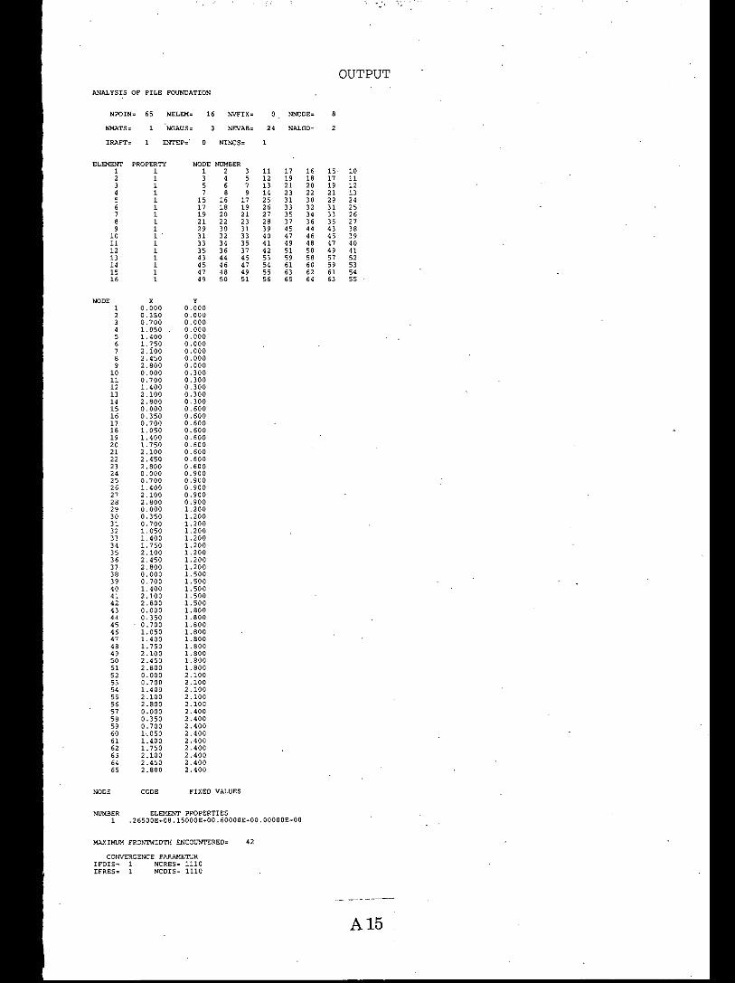
OUTPUTANALYSIS OF PILE FOUNDATION

NPOIN", 65 NELEM" 16 WFIX= 0 NNODE= 8

NMATS" NGAUS" NEVAB= " NALGO=

lRAFT= INTEP" NINes=

ELEMENT PROPERTY NODE NUMBER1 1 1 2 3 11 17 16 15 102 1 3 4 5 12 19 18 17 113 1 5 6 7 13 21 20 19 124 1 7 8 9 14 23 22 21 135 1 15 16 17 25 11 30 29 "6 1 17 18 19 26 33 32 11 257 1 19 20 21 27 35 34 33 268 1 21 22 23 28 31 36 35 279 1 29 30 11 39 45 •• 43 J810 1 11 32 33 40 47 46 45 3911 1 33 34 35 41 49 48 47 4012 1 35 36 31 42 51 50 49 4113 1 43 •• 45 53 59 58 57 5214 1 45 46 47 54 61 60 59 5315 1 47 48 49 55 63 62 61 5416 1 49 50 51 56 65 64 63 55

NODE X Y1 0 000 .0002 0 .350 ,0003 0 700 .0004 1 OSO .0005 1 400 ,0006 1 750 O. 0007 ,. ioa 0.0008 2.450 0.0009 2.800 0.00010 0.000 0.30011 0.700 0.30012 1. 4.00 0.30013 2:.100 0.30014 2:.800 0.30015 0.000 0.60016 0.350 0.60017 0.700 0.60018 1. 050 0.60019 1. 400 0.60020 1.750 0.60021 2: .100 0.60022 2.450 0.6002J 2.800 0.600

" o. 000 0.90025 0.700 0.90026 1. 400 0.90027 2:.100 0.90028 2.800 0.90029 O. 000 1.20030 0.350 1.20011 0.700 1.20032 1.050 1.20033 1. 400 1.20034 1.750 1.20035 2:.100 1.20036 2.450 1.20031 2:.800 1.200J8 O. 000 1.50039 0.700 1. sao40 1.400 1. 50041 2.100 1. 50042 2.800 1.50043 0.000 1. 800•• 0.350 1.80045 0.700 1. BOO46 1.050 1.60047 1.400 1. 60048 1.750 1.60049 2.100 1. 60050 2.450 1. 60051 2.800 1. 60052 0.000 2.10053 0.700 2.10054 1.400 2.10055 2.100 2.10056 2.800 2.10057 0.000 2.40058 0.350 2.40059 0.700 2.40060 1'.050 2.40061 1.400 2.40062 1.750 2.40063 2.100 2.40064 2.450 2.40065 2.600 2.400

NODE CODE FIXED VALUES

NUMBER ELEMEr.--r PROPERTIES1 .26500E .•08 . 15000E .•00 .60000E .•00 OOOOOE.•OO

MAXIMUM FRONTWIDTH ENCOUNTERED= 42

CONVERGENCE PARAMETERIFDIS= 1 NCRES= 1110IFR,ES= 1 NCDIS= 1110

A15

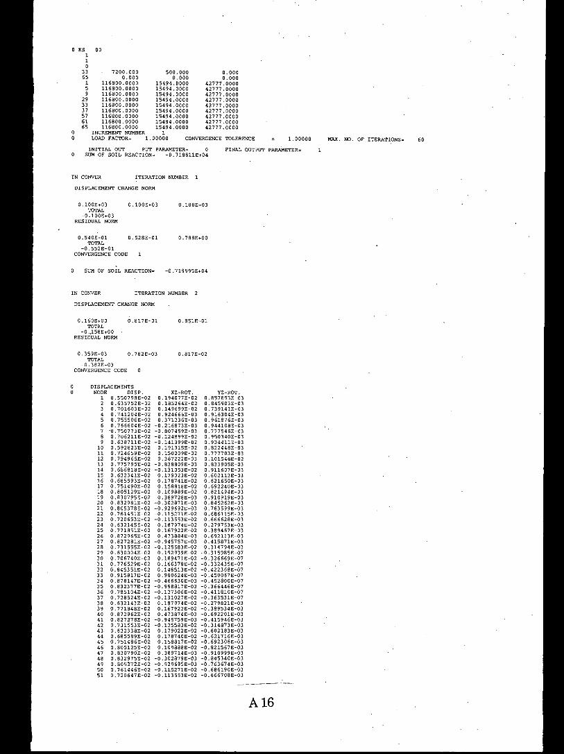
00

INITIALOUT PUT PARAMETER", aSUMOF SOIL REACTION", -0.718811£+04

60MAX. NO. OF ITERATIONS"1.00000

A16

FINAL OUTPUT PARAMETER"

o. 0000.000

42777.000042777.000042777.000042777.000042777.000042777 .000042777 .000042777 .000042777.0000

YZ-ROT..857893E-03845903E-03.739141E-0)9163048-03

0.961876£-030.944108£-030.777546E-030.950340E-030.9344118-030.822448E-030.777703E-030.1015468-020.833905E-030.9116078-030.602113E-030.6216508-030.692240E-030.821494E-030,9109198-030.845262E-030.7635998-030.686115E-030.6666288-030.2797538-030.389467E-030.692113E-030.4158718-030.3147948-03

-0.315985E-07-0.3266698-07-0.3324358-07-0.422368E-07-0.4500678-07-0.452800E-07-0.366446£-07-0.411810E-07-0.3635318-07-0.2798218-03-0.3895348-03-0.6922018-03-0.415946E-03-0.314873E-03-0.6021838-03-0.6217168-03-0.692306E-03-0.821567E-03-0.9109998-03-0.8453408-03-0,7636748-03-0.686190E-03-0.6667088-03

CONVERGENCE TOLERENCE

o .100E .•.03

0.788E .•.00

0.817E-02

0.851E-01

-0.719995£ .•.04

XZ-ROT.194077E-02,185264E-02.149699E-02

0,9246668-030.371236£-03

-0.216873£-03-0.807459£-03-0.124899E-02-0.14.1399E-020.191315E~020.1502098-020.367222E-03

-0.838809E-03-0.1310538-020.179023E-020.178741E-020.158818£-020.109889E-020.3897288-03

-0.302871E-03-0,929692£-03-0.115271E-02-0.113553£-02o ,187974E-020.167922£-020.4738848-03

-O,945757E-03-0.125583£-020.1929398-020.1894718-020.166378£-020.1485138-020.900624E-03

-0.4666308-03-0.998817E-03-0.127306£-02-0.1310278-020.1879748-02o .167922E-020.473874£-03

-0,945759£-03-0,125583£-02o .179022E-020,1787408-020.158817£-020.109888£-02o .389714E-03-0.302879£-03-0.929695£-03-0.115271£-02-0.1135538-02

ITERATION NUMB£R

IT£RATION NUMBER

7200,000 500,0000.000 0.000

116800.0000 15494.0000116600.0000 15494.0000116800.0000 15494.0000116800.0000 15494.0000116800.0000 15494.0000116800,0000 15494.0000116800. 0000 15494.0000116800. 0000 15494.0000116800.0000 15494.0000

INCREMENT NUMBER 1LOAD FACTOR; 1.00000

DISPLACE:M£NTSNODE DISf'.

1 O. 550798E-022 0.635752£-023 O. 701603E-024 0,741204£-025 O. 755506E-026 O. 766604E~027 '0.750773E-028 0.706211£-029 O. 638711E-02

10 0.592823E-0211 0.724659E-0212 O. 794.965E-0213 0.775795E-0214. O. 686818E-0215 0.62234.1E-0216 O. 685593E-02170.7514.90E-0218 0.805129E-0219 O,830795E-0220 O. 832981E-0221 0.805378E-0222 O. 761451E-0223 0, 720653E-0224 0,632145£-0225 O. 771851E-0226 0.872965E-0227 0,827281£-0228 O. 731555E-0229 O. 630004E-0230 O. 706740E-0231 0.776529E-0232 0.845351E-0233 0.915817E-0234 0.878147E-0235 0, 832377E-0236 0,785104£-0237 O. 728524E-0238 O. 632143E~0239 0, 771848E-0240 0.872962E-0241 0.827278E-0242 0.731553£-0243 0.622338E-0244 O. 685589E-0245 O. 751486E-0246 0.805125.£-0247 0.830790E-0248 0.832975£-0249 0.805372£-0250 0.7614468-0251 0.720647E-02

"11o

336515,"3337576165

a .100E+03 O.100E+03TOTAL

~o.100E+03RESIDUAL NORM

DISPLACEMENT CHANGE NORM

SUM OF SOIL REACTION:

DISPLACEMENT CHANGE NORM

0.160E+00 0.817E-Ol'TOTAL

-0.,158E+00RESIDUAL NORM

o .359E-03 .782E-03TOTAL

-0.382E-03COtNERGENCE CODE

0.5408-01 528E-OlTOTAL

~O.552E-OlCONVERGENCE CODE

IN CONYER

IN CONVER

-0.822507E-03-0.777767E-03-0.1015538-02-0.833974E-03-0.911674E-03-0.857937E-03-0.845966E-03-0.7392078-03-0.916368E-03-0.961940E-03-0.944176E-03-0.717615E-03-0.9504128-03-0.934462E-03

X-MOMENT-0.77533E+020.299048+030.722198+030.761928+030.755968+030.79900E+030.78754E+030.41250E+030.15722E+02

-0.565418+010.63622E+030.91427E+030.74454E+03o .12777E+Ol-0.52910E+020.208608+030.52143E+03o .87440E+03o .10970E+040.96171E+030.70779E+030.22084E+03-0.10280E+03-0.60483E+020.49324E+03o .15582E+040.548418+03-0.35214E+02-0.25397E+020.26638E+030.31808E+030.70056E+030.20197E+04o .14933E+040.46351E+030.30462E+03

-0.41071E+02-0.60480E+020.493248+03o .15582E+040.548418+03

-0.35211E+02-0.52911E+020.20860E+030.52143E+030.87440E+030.10969E+040.96170E+030.70778E+030.220848+03

-0.10279E+03-0.565978+010.63621E+030.91427E+030.744538+030.12740E+Ol

-0.77524E+020.29905E+030.72219E+030.76192E+030.75596E+030.79899E+030.78753E+030.41250E+03o .15720E+02

Q-X0.32316E+04o .15346E+04o 10454E+03-0.602578+03o 74799E+020.605938+03-0.18801E+03-0.17647E+04-0.36676E+04o .10526E+040.84339E+030.44356E+02-0.873988+03-0.123458+04-0.79862E+03o .27112E+030.13765E+040.44922E+030.33050E+03-0.15172E+03-0.151118+04-0.32426E+030.89545E+03o .63285E+03o .84204.E+03

-0.17788E+03-0.10785E+04-0.71794E+030.17365E+04o .12940E+040.513238 .•.030.30750E+04

XY-MOMENT-0.348288+020.52781E+02-0.18596E+01-0.89055E+020.114578+010.729251::+02-0.66712E+01-0.756078+02o .18557E+020.523401::+02-0.790308+02-0.13736E+020.62681E+02

-0.805418+020.24674E+02

-0.56791E+02-0.16630E+03-0.13943E+03o .14241E+020.14.5331::+030.98975E+020.358048+02

-0.25521£+02-0.654791::+02-0.10068E+03-0.17697E+030.90749E+020.731598+02-0.21515E-02o .16861E-020.48294E-020.487521::-02-0.26855E-02-0.391398-020.178158-020.99182E-04-0.640878-030.65483E+020.100698+030.17698E+03

-0.90751E+02-0.731628+02-0.24674.E+020.56796E+02o .16630E+030.139431::+03

-0.14244.8+02-0.14533£+03-0.98973E+02-0.35804E+020.25526E+02

-0.523348+020.79034E+020.137388+02

-0.626821::+020.80534E+020.34826E+02

-0.52777E+02o .18564E+01o .89054E+02-0.11488E+01-0.729298+02o .66692E+Ol0.756028+02-0.18565E+02

A17

Y-MOMENT-0.102268+03-0.22449E+02-0.515878+02-0.34648E+02-0.97522E+02-0.27980E+02-0.72180E+02-0.53945E+01-0.13802E+030.20250E+03o . 13272E+030.17765E+03o . 12277E+030.21308E+030.51392E+030.47279E+030.40169E+030.38493E+030.29630E+030.4.17508+030.461758+030.53717E+030.56207E+030.46963E+030.624348+030.95794E+030.689358+030.52471E+03o .40720E+030.569298+030.73595E+030.12035E+040.17798E+040.132658+040.78501E+030.61597E+03o .46500E+030.46964E+030.62434E+030.95793E+030.68935E+030.52472E+030.51391E+030.472798+030.40168E+030.384.92E+030.29628E+030.4.1749E+030.461748+030.53716E+030.562058+030.20248E .•.030.132728+03o . 17764E+030.12276E+030.213058+03

-0.10229E+03-0.224508+02-0.515858+02-0.34652E+02-0.975378+02-0.27980E+02-0.72183E+02-0.539358+01-0.13805E+03

Q-Y0.309568+04o .89336E+03-0.95339E+030.65805E+03o .19004E+040.66872E+03-0.10506E+04o .10253E+040.36025£+04o .15707E+040.202988+02o .14578E+040.471998+020.186958+040.46789£+020.612581::+030.97281E+03o .84383E+03o .10083E+040.107361::+04.0.11638E+040.71538E+03o .15431E+03

-0.56083E+03-0.713608+020.37828E+040.134098+03

-0.63952E+03-0.732428-020.109868+020.567631::-020.59814E-02

52 0.5928178-02 0.1913138-0253 0.7246538-02 0.1502088-0254 0.7949588-02 0.3672088-0355 O. 775787E-02 -0. 838815E-0356 0.6868108-02 -0.1310528-0257 O. 550791E-02 0.194076E-0258 0.6357448-02 0.1852628-0259 0.7015948-02 0.149697E-0260 0.7411958-02 0.924651E-0361 0.7554978-02 0.3712238-0362 0.7665958-02 -0.2168878-0363 0.7507638-02 -0.8074518-0364 O. 706201E-02 -0.1248998-0265 0.6387018-02 -0.1413998-02

III 1 1 1 1 1 1 1 1 1 1 1 1 1ONODENO X-COORD Y-CooRD

1 0.0000 0.00002 0.3500 0.00003 0.7000 0.00004 1.0500 0.00005 1.4000 0.000061.75000.00007 2.1000 0.00008 2.4500 0.000092.80000.0000

10 0.0000 0.300011 0.7000 0.3000121.40000.300013 2.1000 0.3000142.80000.3000150.00000.6000160.35000.600017 0.7000 0.6000181.05000.6000191.40000.6000201.75000.6000212.10000.6000222.45000.6000232.80000.6000240.00000.900025 0.7000 0.900026 1.4000 0.9000272.10000.9000282.80000.900029 0.0000 1.200030 0.3500 1.200031 0.7000 1.200032 1.0500 1.200033 1.4000 1.2000341.75001.2000352.10001.200036 2.4500 1.2000372.80001.200038 0.0000 1.500039 0.7000 1.500040 1.4000 1.500041 2.1000 1.5000422.80001.500043 0.0000 1.8000440.35001.800045 0.7000 1.800046' 1.0500 1.800047 1.4000 1.800048 1.7500 1.800049 2.1000 1.8000502.45001.800051 2.8000 1.8000520.00002.1000530.70002.100054 1.4000 2.1000552.10002.100056 2.8000 2.1000570.00002.400058 0.3500 2.400059 0.7000 2.400060 1.0500 2.400061 1.4000 2.4000621.75002.400063 2.1000 2.4.00064. 2.4500 2.4000652.80002.4000

ONODENO X-COORD Y-CooRD1 0.0000 0.00002 0.3500 0.00003 0.7000 0.00004 1.0500 0.00005 1.4000 0.000061.75000.00007 2.1000 0.00008 2.4500 0.000092.80000.0000

10 0.0000 0.300011 0.7000 0.300012 1.4000 0.300013 2.1000 0.300014 2.8000 0.300015 0.0000 0.600016 0.3500 0.600017 0.7000 0.600018 1.0500 0.600019 1.4000 0.600020 1.7500 0.600021 2.1000 0.6000222.45000.6000232.80000.6000240.00000.9000250.70000.900026 1.4000 0.9000272.10000.9000282.80000.900029 0.0000 1.200030 0.3500 1.200031 0.7000 1.200032 1. 0500 1. 2000

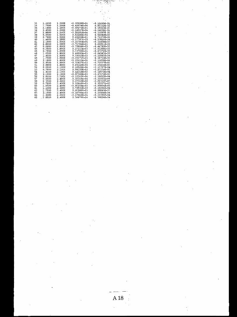
33 1.4000 1.2000 -0.100288 •.04 -0,126958-01

" 1.7500 1.2000 -0.42074E+04 0.903328-0235 :2.1000 1.2000 -0.694768+03 0.184))8-0136 :2.4500 1.2000 -0.1491-7E .•.04 -0.140388-01

" 2.8000 1.2000 -0.20281E+04 -0.115978-0138 0.0000 1.5000 0.632868+03 0.560828+0339 0.7000 1.5000 0.842028+03 0.713708+0240 1.4000 1.5000 -0.17787E+03 -0.378298+0441 :2.1000 1.5000 -0.107858 •.04 -0.13408E+0342 :2.8000 1.5000 -0.717948+03 o .63951E+0343 O. 0000 1.8000 -0.79864E •.03 .-0.467828 .•.0244 0.3500 1.8000 0.271138+03 -0.61258E+0345 0.7000 1.8000 0.137668+04 -0.97278E+0)46 1.0500 1.8000 0.44920E+03 -0.843838+03

" 1.4000 1.8000 0.330458+03 -0.100838+0448 1.7500 1.8000 -0.151738+03 -0.107368 •.0449 2.1000 1.8000 ':'0.151118+04 -0.11638£ .•.0450 2.4500 1.8000 -0.32427£+03 -0.71537£+0351 2.8000 1.8000 0.89542E+03 -0 .15434£+0352 O. 0000 2.1000 0.10526£+04- -0 .15707£ .•.0453 0.7000 2.1000 0.84338£+03 -0.20278£+0254 1.4000 2.1000 0.44346£ .•.02 -0 .14578£+0455 2.1000 2.1000 -0.87398£+03 -0.47172£+0256 2.8000 2.1000 -0.123458+04 -0.186958 .•.045' O. 0000 2.4000 0.32316£+04 -0.30955£+0458 0.3500 2.4000 0.15346£+04 -0.893358+0359 0.7000 2.4000 0.104488+03 0.953378+0360 1.0500 2.4000 -0.60256£ .•.03 -0.65804E+0361 1.4000 2.4000 0.74802£ .•.02 -0 .190048+04-62 1.7500 2.4000 0.605888+03 -0.66869£+0363 2.1000 2.4000 -0.18798£+03 0.10506£+0464 2.4500 2.4000 -0.17646E+04- -0 .102538+0465 .2.8000 2.4000 -0.366768+04 -0.360248+04

A18

Appendix BSome Additional Figures

Figure B.l Nodal moments Mx (lb-ft/ft) along section CD computed fromGauss point values using smoothing technique for simplysupported slab under distributed loading for two differentmesh arrangements.

Bl

276S

2524

2830

23

o@

2630

(a) 2x2 mesh

(b) 5x5 me8h

2385

22

o

1345

21

191

210

216

645 1240 1624 2001 2234 2456 2082 2695 2/38* * * * * * * * * * * * * ~:

177 465 1110 1321 1622 1919 2049 2232 2407 2481 2579 2669 2702 2735 2760* 0 * 0 0 0 .;:

0 ~;

176 639 11012673 2707 2731

* * * * ~: ~;

174 629 1082 2616 2649 267241

41

41

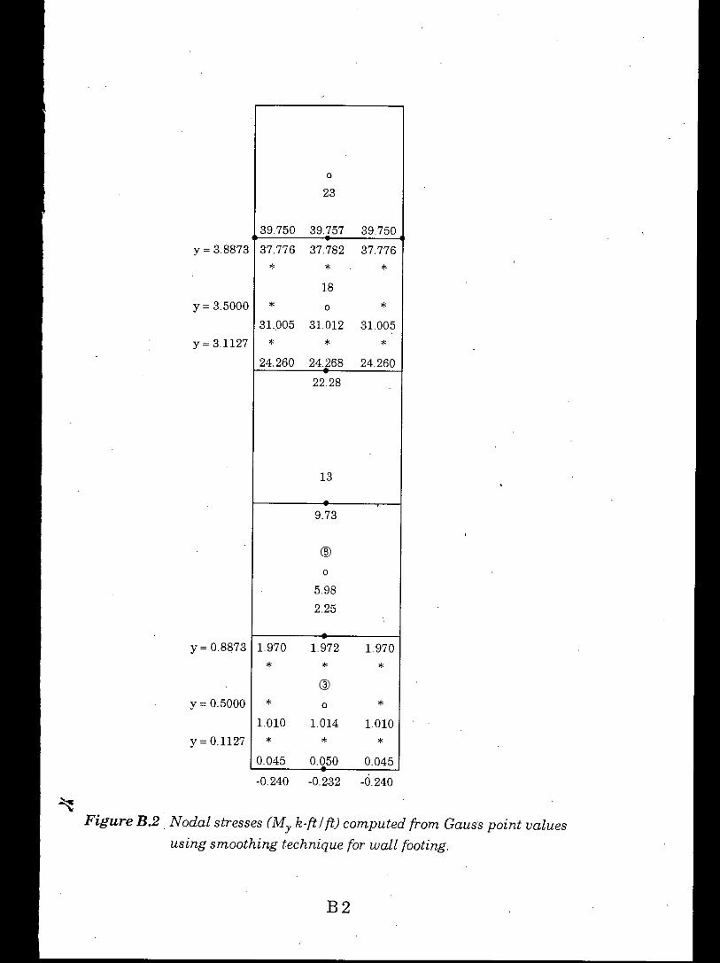
-0.240 -0232 -0240

B2

0

23

39750 39.757 39.75037.776 37.782 37.776

* * *18

* 0 *31005 31.012 31005

* * *24.260 24268 24260

2228

13

9.73

@

0

5.982.25

1970 1972 1.970

* * *@

* 0 *1010 1014 1010

* * *0045 0.050 0.045

y = 3.1127

y = 3.8873

y = 3.5000

y = 08873

y = 0.1127

y = 0.5000

Figure B.2. Nodal stresses (My k-ftlft) computed from Gauss point valuesusing smoothing technique for wall footing.

B3

1.05 1.09 1.07

0

23

20.36 20.34 2038.1863 1868

* *0

17.83

* 18 *1702 1698

1526

0

125513

9.88

0

7.36@

4.81 4.83 4.823.17 319

* *0

@

* *1.66 1.65

y~07887

y~37887

y~0.2113

y~321113

Figure B.3 Nodal shear Qy(k/{tJ computed from Gauss point values usingsmoothing technique.

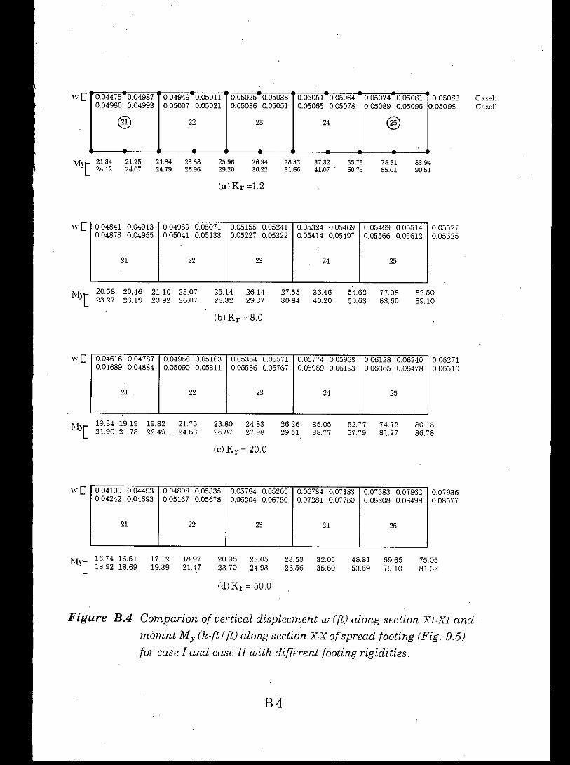
Figure BA Comparion of vertical displecment w (ft) along section Xl-Xl andmomnt My (k-ftlft) along section XX of spread footing (Fig. 9.5)for case I and case II with different footing rigidities.

B4

easel-easel!-

0.055270.05625

0.062710,06510

0.05083.05098

0.079360.08577

75.0581.62

83.9490.51

82.5089.10

80.1386.78

69.6576.10

78.5185,01

77.0883.60

74.7281.27

48.8153.69

54.6259.63

55.7560.75

52.7757.79

37.3241,07 •

32,0535.60

36.4640.20

35.0538.77

23.5326.56

28.3331.66

27.5530.84

26.2629.51

26.9430.22

22.0524.93

26.1429.37

24.8327.98

25.9629.20

20.9623.70

Ca)Kr =1.2

(d)Ki = 50.0

25.1428.32

23.8026.87

(h) Kr =8.0

(e) Kr = 20.0

23.8826.96

18.9721.47

21. 7524.63

21.8424.79

17.1219.39

21.2524,07

21.3424.12

20.58 20.46 21.10 23.0723.27 23.19 23.92 26.07

19.34 19.19 19.8221.90 21.78 22.49

16.74 16.5118.92 18.69

0.04616 0.04787 0.04968 0.05163 0.05364 0.05571 0.05774 0.05963 0.06128 0.062400.04689 0.04884 0.05090 0.05311 005536 0.05767 0.05989 0.06193 0.06365 0.06478

21 22 23 24 25

0.04475 0.04987 0.04949 0.05011 0.05025 0.05038 0.05051 0.05064 0.05074 0.050810.04980 0.04993 0.05007 0.05021 0.05036 0.05051 0.05065 0.05078 0.05089 0.05096

@ 22 23 24 @

0.04109 0.04493 0.04898 0.05335 0.05784 0.05265 0.06734 0.07183 0.07583 0.078620.04242 0.04693 0.05167 0.05678 0.06204 0.06750 0.07281 0.07780 0.08208 0.08498

21 22 23 24 25

0.04841 0.04913 0.04989 0.05071 0.05155 0.05241 0.05324 0.05469 0.05469 0.055140.04873 0.04955 0.05041 0.05133 0,05227 0,05322 0.05414 0.05497 0.05566 0.05612

21 22 23 24 25

w[

w[

w[

w[

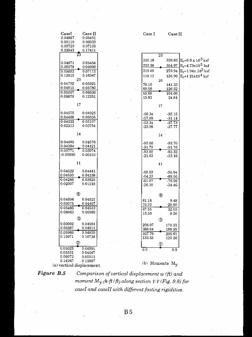
B5

Comparison ofuertical displacem'ent w (ft) andmoment My (k-ft / ft) along section y-y (Fig. 9.8) for

easel and casell with different footing rigidities.

Ec=9.8 x 10 5 ksfEc=4.73x105 ksfEc=1.94x 105 ksfEc=1.21x104 ksf

00

Case IICase I

Ib) Moments My

00

23225.18 326.8322336 • 304.97 -215.09 270.94119.12 136.90

2070.10 141.3369.58 126.5265.68 104.0915.83 24.81

17

-60.34 -2515.57.95 -3114-53.34 -3773-23.98 -27.77

14 .

-95.00 -93.76-91.79 -91.76-8360 -85.32-21.03 -2316

11

-6503 -95.94-64.23 -8856-61.07 -76.50-26.30 -2446

@8118 9487652 ,20.8067.55 32.5513.50 8.50

@29807 17023288.04 18895267.79 205.61133.55 120.26

@

Case II0.054510060330.07195017411

Casel0.048870.051100.05729013543

23

0.04871 0.054340.05078 0059980.05652 0.07112012515 0.16347

200.04792 0.053210.04915 0.057800.05267 0.066360.08870 012251

17

0.04575 0049250.04468 005035004223 0.051070.02213 0.03754

14

0.04490 0.045760.04284 0.044210.03771 0.03974-0.00090 0.00103

. 11

0.04622 0.04441004533 0.042380.04288 0.038250.02007 0.01218

@0.04896 0.045210.05075 004467005486 0.045420.08963 0.06988

@0.05002 0.045840.05287 0.046110.05969 0.049200.13071 0.10738

@0.05023 0.046010.05331 0.04647006072 0.050110.14267 0.11887

Ca)vertical displacement

Figure B.5

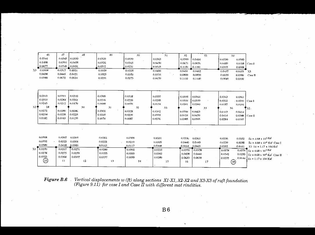
:\':3Case n

Case I

0.0-1-530,05800.0550

0,0457O.OG:,50,0810

0.0462

0.08200.1440

(U).;JSI

0,08000.1-110

0.04000.05350.0670

0.03550.03530.0273

0.03290,032.10.0291

0.03210.04210.0624

0.0317

0.04450,0(,72

46 -17 -IS 49 50 51 52 53 S-J0.03-14 (1.0343 0.0339 0,0329 O.O:B9 0.036..1 0,0399 0.0404 n.0390 O.03R30,0-198 O.03YI O.04S,'~ 0.0:\26 0.0315 o.l)..j.'m o,OG71 o.o67(j O.O;18Y n,O...HJR0,0677 0.0749 0,0691 0,0312 0.0231 0.05.:13 0.1181 0.1181 0.0553 0.0308

(, 11<1')1 " {I':>"" " ,,",,~ " •...•c," " " •. -. - - .~- -X3 0.03080.04380.0588

Case I

X2.

Case II

0.0313 a.mll 0.0310 0.0309 0.0318 0.0337 0.0355 0.03GO 0,03('.1 0.03610.0313 O,OZ84 n.02Gl 0.0116 0.0220 0.0288 n.ll3.'>-t 0.0359 0.0322 0.02910.0243 0.0212 1).017') O.OORS 0.0070 0.0154 (Ul30] 0.0300 O.OIS7 (UllO-~

"2S 30 " 32 33 .35 36

0,0272 0,0280 0.0286 0.0302 UJJ328 0.0362 0.0394 0.0403 0,0 ..-1.13 0.()...J140.025-:1 0,0238 0.0225 0,0205 0.0239 0.0335 0,0424 OJ439 O.()...J14 0.03880.0182 0.0163 0,0139 0.0074 0.0087 0.0236 U.0385 0.0393 0.0284 0.0197

X2

Ec :;:4.68 x 105 Ksf

Ec:;: ..:1.68.'\ .104 Ksf Case I

XI Ec:;:1.17xl04Ksf

Ec :;:4.68 x 105 Ksf

Ec :;: 4.68.'( 104 Ksf Case II

Ec:;: 1.17.x I04Ksf

0.0352

0,02880.0161

0.0356

(lO]39O.030?

U,0361

0,0449

0.0663

0.0356

0.04-100.0664

tl.033 I

0.03(1)0.0308

ll.0309

0.02190,0117

0.0301

0.02230.0165

0,0305

0,03010,0383

0.0307

0.03230.04(8V.U.'U ••• .-...~ "''' •.' v•••• v•• _ ..

" •.'--- v.,,.~.......•V.vV".' --- •..~- ~",' ._.(J.(J259 ll,0267 0,0271 0,0280 0.0302 ,0,0335 0.0370 0,0378 U.tB7M 0,U3760.0278 (J.0275 0.0259 (1.0193 0,0203 0.0302 O,O.US 0.04+1 0.0342 0.02930.0333 0.036S 0.0337 0.0137 (l.D099 0.0289 0,0639 0.0638 0,0292 O.ol4-l@ " 12 13 14 15 IG 17 @

O.fHOB

0.03320.0389

XI

FigureB.6 Vertical displacements w (fO along sections Xl-Xl, X2-X2 and X3-X3 of raft foundation(Figure 9.11) for case I and Case II with different mat rindities.

B6

Figure B.7 Vertical di.\plieel1lenrsw (/i) along see!ions Y]"Y], Yr Y2, Y-,"Y-, and Y4" Y4 ofraftfounda!ion (Fig. 9.11) for ease 1and c'ase11with differenll1lat rigidifies.

B7

Ec ::::4.68 x lOSEc '" 4.(,8.,\ 104

Ec'" 1.17.'\ 104

Ec '" 4.(;8 x lOSEc '" 4.fiX x 104Ec'" 1.17 x Ilr.!.

Ec in kilt"

O.W::>:?0.04()()0.0324

0.045.1-0.05890.056R

0.04550.05800.0550

0.04.150.05350.0457

0.0-l140.03870.0197

).03860.03050.0129

).03970.03280.OI29

0.03760.0293O.OI4-l-

0.03660.02840.015.1-

0.03550.02710.0144

Cast: I Cast: II\"4

0.0;,5-10.03200.0210

Case I Case 11

'""

(J.()3:.(-! O.03:.'J0.0374 0.03280.03(,5 0.02%

Cast: I Case IIY,

(1.03:.9 0.03560.04(,() 0.04240.0644 0.0575

0.0402 0.0409 0.0465 0.0392 0.0459 O.O3~0.0548 0.0740 0.0878 0.0502 0.0670 0.04140.0709 51 0.1407 0.1655 53 0.0591 O.Ol'l.'>4 54 0.0320

a.04OO 0.0403 O.043~ 0.0390 0.0457 O.Q3K30.0535 0.0690 0.0827 O.04WJ 0.06.'>5 0.04080.0670 0.1237 0.1480 0.0553 0.0810 0.0308

0.0392 O.03Ki O.()4..l.7 0.0378O.Q4R.:I 0.0445 0.05% 0.03770,055..1 0.0451 O.OIl70 0,0248

42 43 44 45

0.0378 0.0371 0.0419 0.0373 O.()..lJ2 0.03700.0406 0.0439 0,0543 0,0377 O.(J:'i05 0.03330.0370 0.0488 O.O(>4{) n.D2')l O,04S4 {U1l6•.'!

0.0363 0.0:1(\.1 n.()-H3 O.O31'l}0.0335 0,0322 0.0414 0.02910.023/l 0.0 I 'irl O.02x.J. O.OI(}.+

33 34 35 3(l

0.0349 0.035:!. O.03M-l- 0.035(, 0.0396 0.03:i5 I0,0295 0.034:!. 0.03811 0,0301 0.0357 0.02(>80.01% 0.0309 0.034(, 0.0177 0.0!19 o.oo~0.0342 0.0355 O.()3~(; 0.035! I0.02')4 (Ul316 O.03-l5 0.02740.0241 0.0244 (l.1l25! 0.0120

24 Z5 !(, 27

0.0335 0.0360 0.0375 0.03.-)(, 0.037~ 0.03520.0302 0.0453 O.0-l51 0.0339 0.0342 (Ul2&!0.0289 0.0699 O.OIl74 (I.O:H2 n.0292 0.0161

15 " 17 '"0.0328 0.0362 0.03(>l:l 0.0357 0.03(k~ 0.03530.0309 0.0486 0:0465 0.03(H- O.03 ..U 0.03070.0320 0.0776 0.0725 (J.03(>I'i (J.031') 0.0197

@ !J) @ @YI Y, 1"3

" " ", '"

0.03310.02700.0170

0.03470.03410.02lrl

0.03570.04070.0443

0.03(.•.10.04500.0543

o.o:no0.02880.0241

Cast: I Cast: IIY,

0.03550.0288O.oI~

0.03650.Q4(.•.10.0580

0.03320.03330.0361

0.0:331 0.03200.0343 0.03W0.0360 0.0302

0.03310.03090.0308

-Ui .7 .s 49 :'0 :'1 :'2 :,J 54(LO Ci2.'J1l (;H.12 48.79 -2('.71 -HR5-1 -9J.72 -J9.ril) 79.71 22-1.1-1 2-17.70 224JiH 81. IS -2(i57 -GO.,) IIl.U (ill. 1 I G-I.IS 57.19 7.(J-I -G2.87 -73.-l11 -n.99 (;fUl4 177.-15 17:'.13 174.27 5(,.77 -:>3.21 -80.580.0 50.69 -11.01 50.08 20.92 -Iun -49.64 -4H.18 53.02 12(i.12 94/;5 12-4.95 ~IR.77 -54.% -G2.19

\:3 0.0 :'9.72 62.95 42.05 -3.:1.82 -89.13 -84.11 -22.56 W-I.97 2:'1.89 277.31 256.25 113.31 11.33 -21.28D.O 57.57 60.17 :,LlO -2.72 -66.73 -74.09 -43.nl 79.26 186.81 18..1-.96 185.81 63.86 -41.06 ..70.270.0 49.23 39.24 .:16.79 15.30 -44.44 -52. J I ..51.33 GI.98 133.82 Illl.S9 137.43 5.-1.45 ..50.05 -64.74

1~=.:t.(iHx 10:>ksf

Ec :;:-1.G8:'1 104 ksf Case I

Ec:;: 1.17.>; 10''' ksf

\:3 Ec = 4.G8;o; 105 lesf

Ec = 4.68 ..••104 IesfCase IIEc= 1.17x 10-1 Iesf

X2

0.0 ..6.68 ..20.37 -58.84 -61.99 ..6.25 5.-I.9-l 56.94 9.93 -23.830.0 .(t07 ..5.14 -32.81 -42.25 ..6.10 36.23 34.30 -12.08 ..--13.17(J.() 2.24 1.59. -1.36 ..22.7-1 -5.82 19.33 18.45 ..10.00 ..28.-1:'

28 30 31 32 :n 3:' 3G X2(UI -8.9-1 ..24.28 ..57.87 ..51.(,4 10.22 76.79 81.05 38.20 6.260.0 ..1.56 ..8.03 -34.56 -41.12 ..3.84 40.16 38.93 ..7.00 -38.12o.n 1.7-1 0.60 ..14.14 -23.21 -5.80 21.70 21.35 ..9.44 ..30.06

Ec = 4.68 x 105 IesfEc =4.68 ..••104 ksf Case I

Ec'= 1.17.>; 10-1 ksf

Ec = --1.68 x 105 ksf

Ec = 4.68;0; 104 ksf Case II[c=I.17;o;IO-I ksf

..-10.--11 f'-c =4.68 x 105 ksf

-56.16 Ec=4.68 ..••I04 IesfCasel-40.12 XI Ec = 1.17 x 104 ksf

Ec = 4.68 x 105 ksf

Ec = 4.68 x 104 ksf Case IIEc = 1.17:t 104 ksf

..12.05

..33.87

32.58

47.3-1

31.96

29,(>4

128.:n

95,0('

68.04

137.6(,

&-1.82

39.11

126.48

97.02

68.90

46.88

--11.70

32.28

..27.30

-27.39

"7.73

..74.02

-51.98

31.99

..70.84

-45.30

27.30UI8

..32.23

2.02

13.10

25.75

"5.&-1

26.3028.45

16.76

26.68

30.48

"7.66_ ..~~ .~,~ .•...•.•.....• , '. '" - -' ..~~ - .. '.'.' -_._~ .... " - .. , ... ..~.~~ "'~.'I""T _ .. -

0.0 25.81 24.01 11.29 -37.20 ..67.91 ..65.32 -13.76 63.52 141.82 151.62 143.97 61.11 5.81 ..22.600.0 30.00 27.51 24.63 -1.24 .....J.4.49 ..50.06 ..25.66 43.26 97AS 83.88 95.29 30.93 -32.89 .55.540.0 27.24 16.39 25.20 11.80 -25.99 ..30.36 ..27.15 31.58 68.03 38.21 67.16 28.72 -32.38 ..39.60@ II 12 13 I. 15 . 16 17 @

0.0

O.(J

XI 0.0

Figur~ B.B Moments Mx (k-ft 1ft) along sections Xl-Xl, X2-X2 and x3-X3 of rat foundation (Fig. 9.11) foreasel and casell with different mat rigidities.

B8

Figure B.9 Comparasion ofmements My (kftlft) along sections Yl-Yl, Y2-Y2,

Y3-Y3 and Y4-Y4 of raft foundation (Fig. 9:11) for case I and casellwith different mat rigidities_

117.4857.5226.53

.9,05-29.69.22.74

119.98 Ec '"4.68 x 10:")57.57 Ec '"4.68 x 10424.91 Ec '"1.17 x 10~Ec in ksf

38.99.9.39-15.92

.39.73

.44.24

.26.04

-20.55-15.77.3.87

-8.97.5.25-6.79

0.0 0.0Y4

Case I Case IIY4

0.0 0.0Y3

Case I Case IIY3

Case I Case IIyo

0.0 0.0Y2

134.63 326.00 366.94 107.62 156.17 66.6882.18 242.27 257.63 70.33 92.39 34.3648.06 169.52178.66 41.68 55.77 14.14

51 52 53 54

120.99 196.8"238.78 96.52 145.26 693665.20 148.79167.99 56.05 78.43 34.4831.72 103.67117.95 26.63 40.14 19.97

42 43 44 45

6.03 .53.93 .22.59 -1621 19.17 .7.09.22.39 .61.81 -53.14 -28.68 .18.61 -19.27.25.18 .58.15 -57.38 -26.61 .25.97 -16.14

-25.00 -64.36°.42.79 .43.36 -19.90 .33.10-37.10 -60.98 .58.14 .41.88 -39.04 .32.56-28.02 .46.77 -48.62 -29.07 .31.59 -20.10

33 34 35 36

-48.26 -86.95 .75.52 .62.29 -49.51 .52.79-47.34 .72.02.74.91 -50.57 .53.33 -41.44.29.95 .51.54 .54.97 .30.89 .35.04 .21.73

24 25 26 27

-4.56 48.47 42.48 -8.26 .8.31 -20.72.0.31 54.84 39.66 -0.67 .4.91 -11.615.72 49.22 46.19 5.49 4.03 2.37

15 16 17 18

7.82 69.88 69.62 8.02 4.89 .6.199.93 57.80 57.41 10.93 7.42 -2.1710.56 47.79 47.04 11.60 10.04 0.88

@ CD @ @

.6.651.446.08

9.2212.2111.83

0.0 0.0Y1

89.6154.8526.56

Case I Case IIY1

102.2370.3041.62

B9

.19.03-27.89.25.42

.43.51

.39.74-27.43

.60.46-47.51.28.94