finite element analysis of time-dependent ... the outflow velocity distribution. a nine-node,...

Mathematical Modelling, Vol. 7, pp. 469-482, 1986 Printed in the U.S.A. All rights reserved.

0270-0255/86 $3.00 + .W Pergamon Journals Ltd.

FINITE ELEMENT ANALYSIS OF TIME-DEPENDENT VISCOUS FLOWS UTILIZING AN IMPLICIT MIXED INTERPOLATION ALGORITHM WITH A FRONTAL

SOLUTION TECHNIQUE

BRYAN R. BECKER

Associate Professor of Mechanical Engineering Rose-Hulman Institute of Technology

Terre Haute, IN 47803, USA

and

JOHN B. DRAKE

Engineering Physics and Mathematics Division Oak Ridge National Laboratory

Martin Marietta Energy Systems, Inc. Oak Ridge, TN 3783 1, USA

Communicated by E. Y. Rodin

(Received August 1985)

Abstract-A finite element algorithm is described which implements the Galerkin ap- proximation to the Navier-Stokes equations and incorporates five predominate features. Although none of these five features is unique to this algorithm, their orchestration, as described in this paper, results in an algorithm which is not only easy to implement but also stable, accurate, and robust, as well as computationally efficient. The zero stress natural boundary condition is implemented which permits calculation of the outflow velocity distribution. A nine-node, Lagrangian, isoparametric, quadrilateral element is used to represent the velocity while the pressure uses a four-node, Lagrangian, superparametric element coincident with the velocity element. The easily implemented, computationally efficient frontal solution technique is used to assemble the element coefftcient matrices, impose the boundary conditions, and solve the resulting linear system of equations. An implicit backward Euler time integration rule provides a very stable solution method for time-dependent problems. A Picard scheme with a relatively large radius of convergence is used for iteration of the nonlinear equations at each time step. Results are given for the calculation of two-dimensional, steady- state and time-dependent convection dominated flows of viscous incompressible fluids.

1. INTRODUCTION

The numerical prediction of incompressible, two-dimensional, viscous flows is an important area of computational fluid mechanics. Historically, such predictions have been made by using finite difference algorithms to solve the governing Navier-Stokes and continuity equations. Increasingly, the finite element method, which was developed for solid mechanics calculations, is being applied to this area of fluid mechanics. There are skeptics who question the application of this technique to the nonlinear equations of fluid dynamics because of the very complicated matrix equations which must be solved.

However, there are also several important advantages of the application of the finite element method to this branch of computational fluids. This method facilitates the mod-

469

470 B. R. BECKER AND J. B. DRAKE

elling of flow problems in regions with very irregular geometries. Also, nonuniform meshes are easily used which allow for the resolution of flow details in those regions where necessary, while eliminating superfluous detail in other regions of the same computation. The finite element method also facilitates the imposition of certain boundary conditions in a natural way such as the specified stress boundary.

Fix reports that the finite element method can play a decisive role because of hidden instabilities which often arise in fluid calculations due to boundary effects or nonlinear- itieslll. In certain cases these instabilities can be avoided if conservation laws are satisfied. This condition is intimately related to the finite element method because the Galerkin form has the boundary flux conservation built into it.

Taylor and Hood published an early paper on the numerical solution of the Navier- Stokes equations using the finite element technique[2]. Both a velocity-pressure formulation and a stream function-vorticity formulation are presented, and it is reported that the former had some advantages for contained flow problems. Using the Galerkin technique with eight-node isoparametric elements to arrive at the discrete equations, two velocity-pressure formulations are given: one involving a specified stress boundary condition, the other a specified velocity gradient boundary condition. Sample calculations for Couette flow and for the driven cavity problem with Reynolds numbers of 1, 100, 400, and 600 are reported.

Kawahara et al. used the velocity-pressure form of the momentum equations with the specified stress boundary conditions[3]. They employed triangular finite elements, six nodes for velocity and three for pressure with complete second-order polynomial interpolation functions for velocity and complete linear polynomials for pressure. Results for an expanding channel flow with Reynolds number of 150 are given.

Gartling and Becker used the energy balance approach to formulate the finite element equations in terms of the velocity-pressure unknowns with the specified stress boundary condition[41. Eight-node, isoparametric quadrilateral elements and six-node, isoparametric triangular elements were used with quadratic serendipity shape functions for pressure. Results are given for flow in a 90” T-junction Re = 100; driven cavity flow Re = 100; and flow over a circular cylinder Re = 5.

Bercovier and Engelman used a finite element penalty method for the simulation of incompressible viscous flows with the specified stress boundary condition[5]. In this approach, a perturbed system of equations is solved in which the continuity requirement is weakened and the pressure unknown is eliminated. Thus, the size of the global system is reduced by one-third. The pressure distribution is then recovered from the velocity distribution via a post-solution calculation. A nine-node, isoparametric quadrilateral element is used for the velocity unknowns with biquadratic interpolation functions. Results are given for the driven cavity flow Re = .OOl, 100, 400, 1000; flow past a cylinder Re = 75; and time-dependent flow past a square step.

Huyakorn et al. reported a comparison of the performance of four types of mixed interpolation finite elements using the velocity-pressure formulation with the stress boundary condition[6]. Mixed interpolation refers to the fact that these types of elements employ a pressure shape function which is a polynomial of lower degree than that used for the velocity shape function. The elements compared in this study are the six-node triangular element with pressures at the vertices, an eight-node serendipity element with corner pressures, the nine-node Lagrangian element with corner pressures, and a four-node quadrilateral element with the constant pressure “node” located logically at the centroid of the element. Two test cases were employed: steady flow through a sudden expansion and steady free convection in a square cavity. It was found that the nine-node Lagrangian element gave the best results for both pressure and velocity and that the eight-node serendipity element gave the least accurate pressure distribution. The poor performance of

Finite element analysis of time-dependent viscous flows 471

the serendipity element is explained qualitatively by the fact that the pressure variable behaves as a Lagrange multiplier which results in a more highly constrained system of algebraic equations, thus, reducing accuracy. It was also found that unless pressures or total stresses are specified on at least one boundary, the four-node element displayed large oscillations in the pressure field which took the form of a checkerboard pattern. This performance is a result of a spurious pressure which causes the global stiffness matrix to be rank deficient. The solution of this system results in arbitrary amounts of this spurious pressure mode being added to the desired physical pressure solution. Huyakorn et al. also report that the performance of the triangular element is dependent upon the mesh pattern used.

The question of spurious pressure solutions was studied by Fix et a1.[71 and by Sani et a1.[8]. Computationally, the pressure solution is only determined within an additive constant. This can be seen easily from the governing equations since pressure only appears differentiated. Somehow the algorithm must establish a pressure level. This arbitrary level is referred to as the “hydrostatic” pressure mode. The existence of this “hydrostatic” pressure mode implies that the assembled matrix will have a zero eigenvalue corresponding to the redundant continuity equation. In practice, this pressure mode is eliminated by specifying the pressure at one point on the mesh.

Other pressure modes may appear as a linear dependence among the continuity equations. In particular, Sani et al. document the checkerboard mode that other researchers have encountered[8]. There are two methods of dealing with “spurious” modes such as the checkerboard. One method is to choose elements and interpolation functions which will not permit spurious modes. For example, it is recommended that a biquadratic interpolation function be used for velocities and a linear polynomial of the form, a + bx + cy, be used for the pressures. The second method is to smooth the bad results of a poor element in such a way that the spurious modes are filtered out. Explicit formulas for this smoothing and further details are given in the paper by Sani et al.

The finite element algorithm described and discussed in this article incorporates five predominant features. Although none of these five features is unique to this algorithm, their orchestration, as described in this paper, results in an algorithm which is not only easy to implement but also stable, accurate, and robust, as well as computationally efficient. The first of these five features is the use of the zero stress natural boundary condition which permits the outflow velocity distribution to be determined as part of the solution rather than being specified as a boundary condition. This produces an especially useful solution method for those problems in which the outflow velocities are unknown.

The second feature concerns the type of element used to discretize the solution region. In the current algorithm, a middle ground between accuracy and ease of implementation was chosen. The velocity is represented with a nine-node, Lagrangian, isoparametric quadrilateral element. Thus, the velocity is biquadratic over each element as suggested by Sani et ~1.181. The pressure is represented with a four-node, Lagrangian, superparametric quadrilateral element coincident with the velocity element. This combination of velocity and pressure representations results in an easily implemented element stiffness matrix. Also, as observed by Huyakorn et a1.[6], this combination gives good pressure and velocity solutions. Any spurious pressure modes that might arise can be tiltered out by post processing the solution.

The third feature of interest in this algorithm is the use of the frontal solution technique to solve the linear system of equations which results from the finite element discretization. This solution technique, which is based upon the work of Hood[9], handles the assemblage of the element coefficient matrices as well as the imposition of the boundary conditions. Both the assemblage and factorization are accomplished in one pass through the element matrices, thereby eliminating the need to store element matrices out of core. In addition,


this solution technique requires less incore work space than other types of solvers. Hence, the frontal solution technique makes the finite element algorithm described in this article both easy to implement and computationally efficient.

Fourth, the current finite element algorithm incorporates an implicit backward Euler time integration rule which provides a very stable solution method for time-dependent problems. Finally, a Picard iteration scheme is used by the current algorithm to solve the nonlinear equations at each time step. Although this scheme may converge slowly, it has a relatively large radius of convergence so that the algorithm described in this paper is fairly robust.

Further details of these five features and their orchestration in the current algorithm are presented in the following sections of this article. Section 2 gives a discussion of the finite element formulation used in the present code; while Sec. 3 describes the method of time integration and the iteration scheme employed. Section 4 describes the frontal solution technique used to solve the governing system of linear equations which results from the discretization. Finally, Sec. 5 presents the results of sample calculations as well as conclusions concerning the present finite element algorithm for time-dependent viscous flows.

2. THE FINITE ELEMENT FORMULATION

2.1 Continuum problem to be solved

The current program is designed for the analysis of two-dimensional, laminar, iso- thermal, incompressible flows of a single species Newtonian fluid. Furthermore, this analysis is to take place on a closed and bounded region V, with boundary S. The boundary is composed of two distinct portions S1 and S2:

s = s, u sz; (2.1)

and

s, f-l s* = 6. (2.2)

The two types of boundary conditions which may be considered in the current analysis are given as

Ui = OiOllS1, (2.3)

and

Tijnj = 9i on Sz. (2.4)

In Eq. (2.3), Oi is a prescribed velocity component in the xi direction. In Eq. (2.4), Si is the prescribed component of the stress vector exerted in the xi direction across a surface whose outward normal from the fluid has direction cosines nj.

With the assumptions listed above, the momentum equations corresponding to the boundary conditions given in Eq. (2.3) and Eq. (2.4) have the following form:

f’ $f + P%uij = -Fyi + p(Uij + Uj,i),j + pFi, i = 1,2. (2.5)

Finite element analysis of time-dependent viscous flows

Conservation of mass is enforced through the incompressible continuity equation

473

Ui,i = 0. (2.6)

Equation (2.5) and Eq. (2.6) form a set of three continuum equations governing the two velocity components and the flow field pressure. These continuum equations and the boundary conditions given in Eq. (2.3) and Eq. (2.4) are used to generate the set of discrete equations which is presented in Sec. 2.2.

2.2 Formulation of the discrete equations

In the two-dimensional application of the finite element method, the region of interest V, is discretized into a patchwork of two-dimensional cells or elements. The current code uses nine-node, isoparametric, Lagrangian quadrilateral elements for the velocity components and four-node, superparametric Lagrangian quadrilateral elements for the pressures. The variables of interest are then expressed as functions of space within each element via interpolation or shape functions. In the current code the flow pressure is interpolated using complete bilinear polynomials +L (x, y), while the velocity shape functions 4” (x, y), are chosen to be biquadratic.

Applying the Galerkin finite element method to the continuum problem presented in Sec. 2.1 yields a discrete set of equations for the velocity and pressure unknowns. Con- sidered on a single element of the finite element mesh, the momentum equation in the xi direction may be written in the following symbolic form:

MKL au,” - + c”U; - QFJ pJ + Kff vi” at

+ K&= Uf + Si, (Kfi= Vi” + Kg= Ug)

+ Sj2 (K;“= Uf + KF2= Uf) = F:. (2.7)

In Eq. (2.7), J counts the four pressure nodes and K and L count the nine velocity nodes within the element. The discrete continuity equation is expressed symbolically as follows:

0:” Uf + 02” UC = 0. (2.8)

In Eq. (2.8), J counts the four pressure nodes and L counts the nine velocity nodes. These two symbolic equations are then combined to yield a 22 x 22 element stiffness matrix. These element matrices are then assembled to form a global stiffness matrix which rep- resents the discrete form of the continuum problem on the entire region V.

3. THE SOLUTION ALGORITHM

3.1 Time integration for nonsteady problems

After assembling (or summing) all the element matrices into their appropriate location in the global matrix, the global system can be represented as

Mti + C(U)U + KU = F. (3.1)

The matrices, M and C(U), are referred to as the mass matrix and the convection matrix, respectively. The matrix K which contains the pressure terms, continuity and stress terms,


will be called the stress matrix. Equation (3.1) is a system of ordinary differential equations for the unknowns at the node points. The spatial derivatives have all been discretized by the finite element Galerkin method.

Equation (3.1) is solved in the present code by the backward Euler rule. The backward time derivative at time t”+’ is given as

On substituting Eq. (3.2) into Eq. (3.1) and rearranging terms, Eq. (3.1) becomes

E + C(Un+l) + K MU"

Un+’ = F + ht.

(3.2)

(3.3)

The set of equations represented by Eq. (3.3), is solved, as discussed in the next section, to give U at the time t”+ ’ . By using the backwards Euler rule and evaluating the nonlinear convection matrix at the advanced time, the algorithm is fully implicit. Explicit algorithms traditionally require many time steps to maintain stability. Unfortunately they lose accuracy with each time step. The implicit algorithm of Eq. (3.3) is unconditionally stable. Accuracy desired for a particular problem places the only limitation on the size of the time step chosen.

3.2 Solution of the discrete nonlinear equations

Once a solution is obtained at the time r”, Eq. (3.3) can be solved using an iterative scheme to give the solution at time t”+‘. The iterative technique used by the current code is called a Picard iteration. It is the simplest of the fixed-point iteration schemes. Aside from its simplicity, it has the advantage over other schemes of a large radius of convergence so that the present algorithm is fairly robust.

The disadvantage of the Picard iteration is that its asymptotic rate of convergence is only linear. A modified Newton scheme would decrease the number of iterations required to solve the nonlinear system given in Eq. (3.3). In particular, for steady state problems, a quasi-Newton method could be applied after a few iterations of the Picard scheme. For time-dependent problems, the iteration could be initiated at the first time step by the Picard scheme followed by the quasi-Newton method as described for the steady state. Then, at subsequent time levels, the quasi-Newton method could be applied directly by using small enough time steps. With this strategy, a supralinear rate of convergence could be achieved while maintaining the robustness of the overall algorithm. However, the implementation of such an iteration strategy would greatly increase the complexity of the resulting finite element code. For the current algorithm, robustness and ease of implementation of the iteration scheme were chosen over efficiency of convergence.

To write the iteration scheme, let U;+’ denote the solution at time tn+‘, iteration p. Typically, we choose Uo”” = CT”. Then Up+‘, p = 1, 2, . . . is the solution to

E + c(u,“t;) + K MU”

U;+' = F + z . (3.4)

Notice that the nonlinear convection matrix is lagged one iteration. This scheme is re- peated until the solution converges or until some maximum number of iterations has been performed. The convergence of the iteration is measured using the sum of squares of the

Finite element analysis of time-dependent viscous flows 47.5

difference between successive iterates. A convergence tolerance RTOL, is specified and Eq. (3.4) is iterated until:

(3.5)

The number of iterations required to achieve convergence is not only highly problem dependent but in a transient analysis may also vary widely from time step to time step within a single simulation. In general, the number of iterations which are required for convergence depends directly upon the difference between the initial iterate and the converged solution.

In a transient analysis, two parameters influence this difference: time step size and Reynolds number. If a large time step is used, then the state of the fluid at time tn+’ will be much different from that at time t”. Hence, the converged solution at t” which serves as the initial iterate for time tn + ’ will greatly differ from the converged solution at tn+ ‘. Correspondingly, a large number of iterations will be required to achieve convergence at the P+* time step.

The second parameter, Reynolds number, is an indicator of how fast the fluid is moving relative to the scale of the problem. In a transient problem at high Reynolds number, the state of the fluid may change drastically even during a small time step. Thus, as described above, a large number of iterations would be required for convergence at each time step.

Likewise, for a steady state analysis at high Reynolds number, the state of the fluid in the converged solution may be very different from the initial conditions used to start the iteration. Again a slow rate of convergence would be experienced. This convergence rate at high Reynolds number may be greatly improved by using a converged solution at a lower Reynolds number to start the iteration.

The current code takes advantage of the form of Eq. (3.4) to efficiently organize its computations. The mass and stress matrices are only computed once per problem for each element and then stored on disk. The multiplication of M times U” is performed only once per time step and added to F only once per time step. This is possible since the right-hand side of Eq. (3.4) remains the same over the course of the iteration. To form the global stiffness matrix [left-hand side of Eq. (3.4)], the mass and stress matrices are added and stored on disk once per problem. Then, the C matrix is formed at each step of the iteration and added to M plus K.

For steady-state calculations, the mass matrix M, is completely omitted from the global system shown in Eq. (3.1) and from the subsequent equations. The steady-state iteration scheme is then similar to taking a single transient time step.

4. FRONTAL SOLUTION TECHNIQUE

4.1 General discussion

In the current problem each 22 x 22 element stiffness matrix is constructed from the symbolic equations given in Sec. 2.2. A node in the region V may, in general, appear in several of the elements which make up V. Therefore, in order to complete the set of global equations governing the values of the unknowns at a given node, it is necessary to su- perimpose or “assemble” the contributions to those equations from each of the elements in which the node appears. That is, all of the element stiffness matrices from those elements containing a given node must be assembled into a global stiffness matrix before the global equations at that node are complete. One method to perform this task would be to completely assemble all of the element stiffness matrices into a single huge global stiffness matrix and then solve the resulting system for the values of all of the unknowns in the


entire region. This method would, in general, require a very large amount of computer storage. An alternative method would be to assemble only those element stiffness matrices which involve a given node and then eliminate the resulting complete or fully summed equations as they occur in the assembly process. This method, known as a frontal solution algorithm, is used in the current program.

4.2 Description of the frontal algorithm

The current program uses a frontal solution algorithm based upon the work of Hood[9]. This algorithm starts by asking for element stiffness matrices in order of element number. These element matrices are assembled into an incore work space. Assembly continues until the allocated work space is filled, then all of the fully summed rows and columns are searched for the largest entry which becomes the pivot. The fully summed rows and columns are those to which no more entries will be added as the remaining element matrices are assembled. The row containing the pivot is then used to zero the column containing the pivot. All pivotal information is then written to disk storage and the size of the active portion of the incore work space is reduced by deleting the pivotal row and column. This process continues until sufficient space is freed in the incore work space so as to allow for the assembly of yet another element stiffness matrix. This process of assembly followed by elimination of fully summed rows and columns, followed by ad- ditional assembly, etc., continues until all of the element matrices have been assembled and all elimination is complete. Then a back-substitution is performed to obtain the solution.

This algorithm is not only computationally efficient, it also controls the finite element solution. That is, it performs the global assembly, requesting element stiffness matrices as they are needed, which in turn causes the required integration to be performed and the element matrices to be constructed as they are needed. At the same time, the frontal algorithm performs the elimination until the entire system has been reduced. The algorithm then calls for the back substitution which produces the solution. Thus, the frontal algorithm is the central core of the entire finite element problem. A more thorough discussion of this algorithm as well as a listing of the computer routines comprising the frontal algorithm are given in the reference by Hood[9].

5. RESULTS AND CONCLUSIONS

5.1 General remarks

To validate the present code, three test problems were chosen: the driven cavity, the expanding channel, and the Couette flow problem, all of which appear in the literature as mentioned in Sec. 1. A general description of each of these problems as well as the results for a particular test case are presented in this chapter. In these test cases, all physical parameters are considered to be in a consistent system of dimensional units. A discussion of the accuracy of the current code and some general conclusions follow the presentation of the results.

5.2 The driven cavity

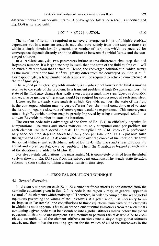
The steady-state driven cavity test problem is depicted in Fig. 1. A pocket of fluid contained in the two-dimensional box is maintained in motion by a flow across the top of the box. The velocity across the top of the box is specified as unity in the horizontal direction. The density and viscosity used in the calculation were 1 .O and 0.5, respectively.


” = .5 v=o

f//////////z

u=v=o

SPECIFIED VELOCITY

NO SLIP BOUNDARY

Fig. 1. Steady driven cavity problem.

The relevant number for comparison with other calculations is the Reynolds number Re = p U11l.q wherein U the characteristic speed of the problem, is 1.0 in this calculation; 1 the characteristic length, is 1.0 for the width of the cavity; and p and TV are the density and the viscosity. The Reynolds number for this problem is then 2.0. In this calculation, 25 elements were used to discretize the region.

The solution of the steady-state driven cavity problem is given in Figs. 2 and 3. The velocity distribution, Fig. 2, depicts the large vortex which exists in the cavity. The steady- state pressure distribution is given in Fig. 3. These results agree well with those found in the literature[2, 4, 51.

5.3 The expanding channel

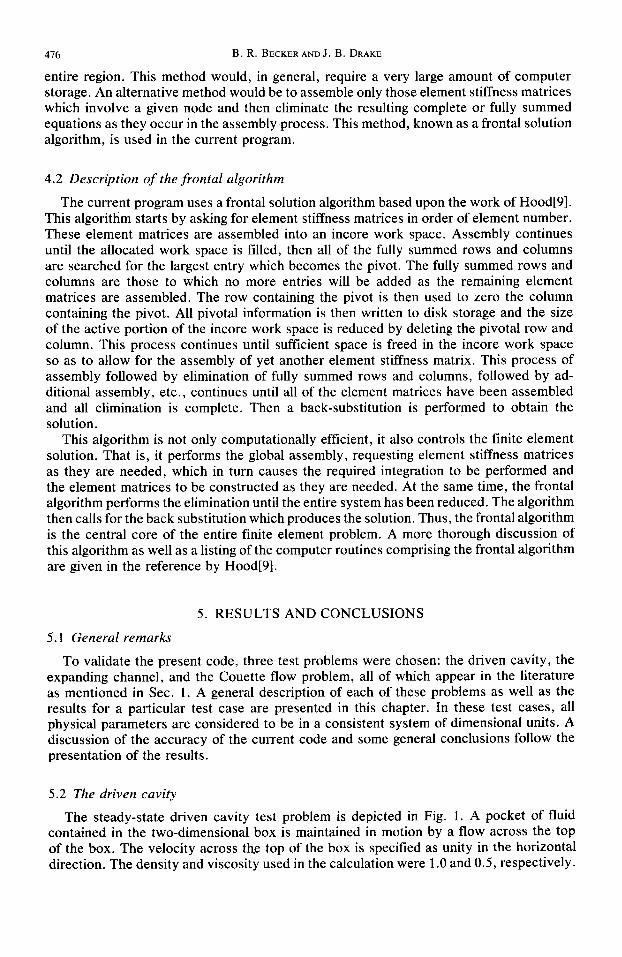
Like the driven cavity, the expanding channel is a steady-state simulation. This problem illustrates the “natural” boundary conditions of the finite element method as applied to fluid dynamics. As shown in Fig. 4, the upper and lower boundaries, which are fixed walls, are treated as no-slip boundaries and thus the velocities are prescribed to be zero there. The fluid enters from the left boundary with a fully developed parabolic velocity profile. The centerline velocity at the inflow is specified to be unity. At the outflow boundary, the stress is prescribed to be zero. This zero stress boundary condition is the natural boundary condition which appears in the Galerkin formulation as the surface integral of the normal stress 7ij nj. Thus, the stress components, 712 and 722, do not enter the problem at all since the normal to the outflow boundary is fi = (1, 0)‘. Since the velocity components are not specified at the outflow boundary, the zero stress boundary condition permits inflow to occur at the outflow boundary. Thus, the outflow velocities are determined as part of the solution which is a desirable situation if they are not known a priori.

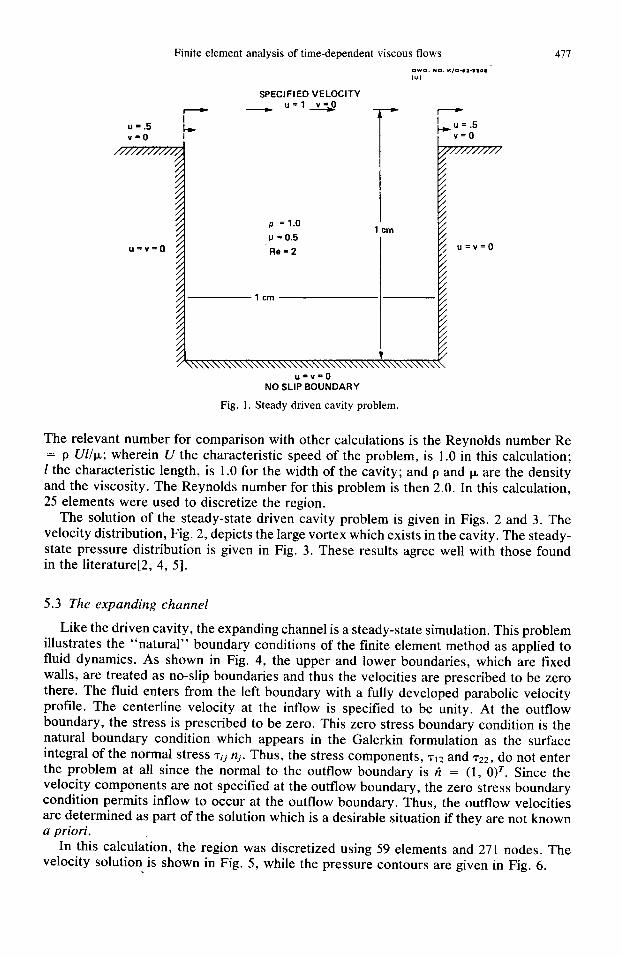
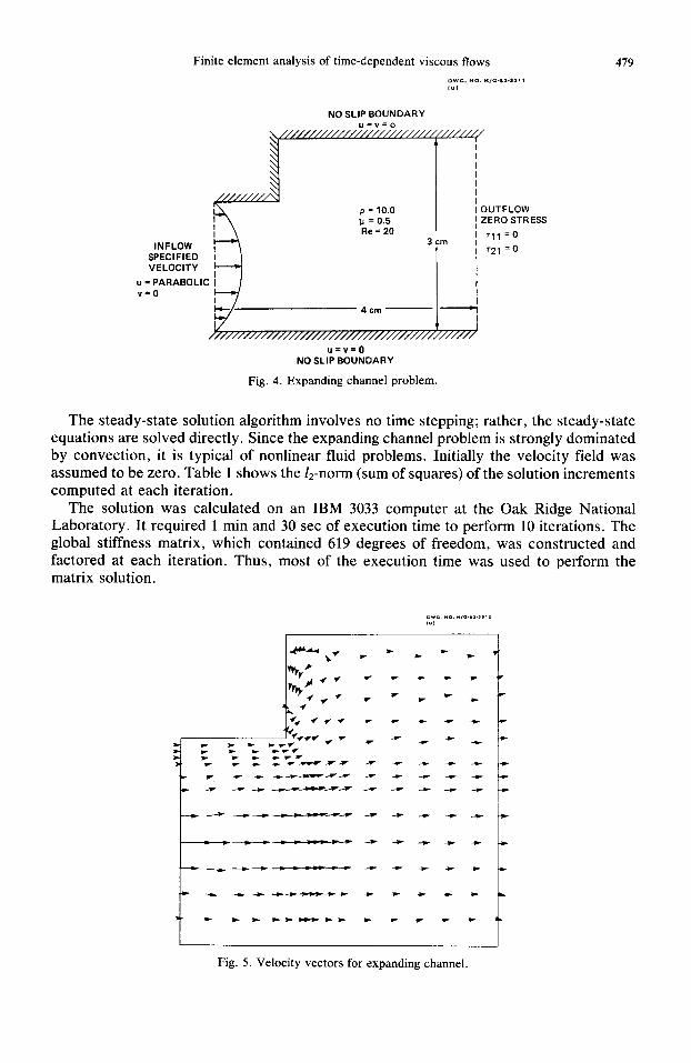
In this calculation, the region was discretized using 59 elements and 271 nodes. The velocity solution is shown in Fig. 5, while the pressure contours are given in Fig. 6.


+

\

b

\

\

\

b

t

Fig. 2. Velocity vectors for driven cavity.

Fig. 3. Pressure contours for driven cavity.


NO SLIP BOUNDARY u=v=o

3

“, I$,ckF$ ,,,,,,,,,,,,,,,,,,,, ~~~ ,,,,,,, 1;

u=v=o NO SLIP BOUNDARY

Fig. 4. Expanding channel problem.

3

OUTFLOW ZERO STRESS

r,, =o

‘2, =o

The steady-state solution algorithm involves no time stepping; rather, the steady-state equations are solved directly. Since the expanding channel problem is strongly dominated by convection, it is typical of nonlinear fluid problems. Initially the velocity field was assumed to be zero. Table 1 shows the 12-norm (sum of squares) of the solution increments computed at each iteration.

The solution was calculated on an IBM 3033 computer at the Oak Ridge National Laboratory. It required 1 min and 30 set of execution time to perform 10 iterations. The global stiffness matrix, which contained 619 degrees of freedom, was constructed and factored at each iteration. Thus, most of the execution time was used to perform the matrix solution.

Fig. 5. Velocity vectors for expanding channel.


Table 1. 1~ norm of increments for the expanding channel

Iteration Norm of Increment

1 7.50 2 4.14 3 3.72 x 10-l 4 3.00 x 1om2 5 4.43 x 10-j 6 7.84 x 1O-4 7 1.50 x low 8 2.86 x 10m5 9 5.13 x 10-6

10 8.62 x lo-’

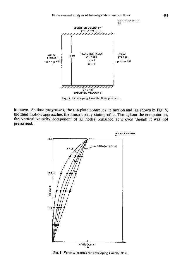
5.4 Developing couette j7ow

Steady-state Couette flow has a simple analytic solution. A time-dependent Couette flow problem is included to show the dynamic capability of the code. The problem is depicted in Fig. 7. A fluid is trapped between two infinite parallel plates; the lower one fixed, the top one moving with a constant velocity. The top and bottom boundaries are taken as no slip boundaries with the velocities prescribed as equal to those of the adjacent plates. The side boundaries are zero stress boundaries as described in Sec. 3. The computational region was discretized into nine elements in 3 x 3 square.

It is assumed that at time zero, the fluid is at rest and that the top plate has just begun

Fig. 6. Pressure contours for expanding channel.

Finite

ZERO STRESS

r,,=7*,=0

SPECIFIED VELOCITY u=l,v=O

-I---

3cm FLUID INITIALLY AT REST

I p =1

!.I = .5

ZERO

STRESS

‘,, = ‘2, = 0

+ z///////////////////////////////////:

U-V=0 SPECIFIED VELOCITY

Fig. 7. Developing Couette flow problem.

to move. As time progresses, the top plate continues its motion and, as shown in Fig. 8, the fluid motion approaches the linear steady-state profile. Throughout the computation, the vertical velocity component of all nodes remained zero even though it was not prescribed.

u VELOCITY 1.0

Fig. 8. Velocity profiles for developing Couette flow.

482

5.5 Concluding remarks

B.R. BECKERANDJ. B. DRAKE

The finite element method as discussed in this paper has several interesting aspects. First, the finite element formulation includes the zero stress natural boundary condition which permits inflow to occur at an outflow boundary. Thus, as shown in the expanding channel and developing Couette flow problems, the outflow velocities are determined as part of the solution. This removes the necessity of specifying velocities at the boundaries which may be unknown.

Second, the use of the biquadratic, Lagrangian, isoparametric, nine-node elements for velocity and bilinear, Lagrangian, superparametric, four-node elements for pressure re- duces program complexity while facilitating the modeling of curved boundaries. Also, as demonstrated by the sample calculations, these elements give realistic velocity and pressure solutions which compare well to those found in the literature. As shown by these three test cases, the pressure solutions are often acceptable with no need to filter out spurious pressure modes.

Third, the backward Euler fully implicit time integration provides a very stable solution method while the Picard iteration scheme insures a large radius of convergence. These two factors make this finite element algorithm both accurate and robust.

Fourth, the use of the frontal solution technique to assemble and solve the linear system of equations is not only very computer efficient but also very easy to implement. The frontal solution algorithm is the central core of the entire finite element program, it performs the global assembly, requesting element stiffness matrices as they are needed. Thus, it causes the required integrations to be performed and the element matrices to be constructed. At the same time, this solution technique performs the elimination until the entire system of equations has been reduced. It then calls for the back substitution which produces the solution.

In summary, the results of the sample calculations have demonstrated the usefulness of the present finite element algorithm for the numerical solution of steady-state and time- dependent problems in the realm of viscous flows. Also, the present work has demonstrated the ease of implementation afforded by the frontal solution technique which when coupled with Picard iteration and backward Euler time integration provide for a robust and accurate algorithm.

1.

2.

3.

4.

5.

6.

7.

8.

George J. Fix, Finite elements and fluid dynamics, ICASE Report number 75-1, NASA Langley Research Center, Hampton, Virginia, February 1, 1975. C. Taylor and P. Hood. A numerical solution of the Navier-Stokes equations using the finite element technique: Compur. FIuids 1, 73-100 (1973). M. Kawahara, N. Yoshimura, K. Nakagawa and H. Ohsaka, Steady and unsteady finite element analysis of incompressible viscous fluid. Inr. J. Numer. Merh. Engng 10, 437-456 (1976). D. K. Gartling and E. B. Becker, Finite element analysis of viscous incompressible fluid flow. Comput. Meth. Appl. Mech. Engng 8, 51-60, 127-138 (1976). M. Bercovier and M. Engelman, A finite element for the numerical solution of viscous incompressible flows. J. Comput. Phys. 30, 181-201 (1979). P. S. Huvakom. C. Taylor, R. L. Lee and P. M. Gresho, A comparison of various mixed-interpolation finite elements-in the velocity-pressure formulation of the Navier-Stokes equations. Comput. Fluids 6,.25-35 (1978). G. J. Fix. R. A. Nicolaides and M. 0. Gunzburger. On mixed finite element methods for a class of nonlinear boundary value problems. In Computational Methods in Nonlinear Mechanics, Chap. 10, North-Holland, Amsterdam (1980). R. L. Sani, P. M. Gresho, R. L. Lee and D. F. Griffiths, The cause and cure (?) of the spurious pressures generated by certain FEM solutions of the incompressible Navier-Stokes equations. Inr. J. Numer. Mefh. Fluids 1, 17-43 (1981).

9. P. Hood, Frontal solution program for unsymmetric matrices. In?. J. Numer. Merh. Engng 10,379-399 (1976).

REFERENCES

finite element analysis of time-dependent ... the outflow velocity distribution. a nine-node,...

Documents