DEStech Publications, Inc.

THE MECHANICS OF ADHESIVES IN COMPOSITE AND METAL JOINTSFinite Element Analysis with ANSYS

Magd Abdel Wahab, Ph.D.Professor and Chair of Applied MechanicsGhent University

stnioJ lateM dna etisopmoC ni sevisehdA fo scinahceM ehT

hcetSED .cnI ,snoit ac il buP teertS ekuD htroN 934

.A.S.U 20671 ain av lys nneP ,ret sac naL

thgir ypoC © yb 4102 hcetSED .cnI ,snoit ac il buP devres er sthgir llA

a ni derots ,decud orp er eb yam noit ac il bup siht fo trap oN ,snaem yna yb ro mrof yna ni ,det tim snart ro ,met sys laveirt er

,esiw re hto ro ,gni droc er ,gni ypoc ot ohp ,lac i nahc em ,cinort cele.rehsil bup eht fo nois sim rep net tirw roirp eht tuo htiw

aci remA fo setatS detinU eht ni detnirP1 2 3 4 5 6 7 8 9 01

:elt it red nu yrt ne niaM SYSNA htiw sisylanA tnemelE etiniF :stnioJ lateM dna etisopmoC ni sevisehdA fo scinahceM ehT

A hcetSED koob snoit ac il buP .p :yhp ar go il biB

512 .p xed ni sedulc nI

0536394102 :rebmuN lortnoC ssergnoC fo yrarbiL9-690-59506-1-879 .oN NBSI

ix

Preface

ADHESIVE BONDING TECHNOLOGY is a powerful joining technique, especially for thin sheets of metal or composites. The superiority

of adhesive bonding is manifest in its high fatigue resistance and high strength-to-weight ratio. Since an adhesively bonded joint consists of different materials, its structural analysis is complicated and requires many special considerations and assumptions. For instance, when ad-hesives are used to join thin sheets, large deformation behavior is ex-pected under thermal and mechanical loads. In addition, modern adhe-sives display significant degrees of plasticity, which further complicates analysis. For an analysis of this kind that includes diverse materials and geometric non-linearities, a reliable analytical solution is almost impossible.

Numerical techniques, such as Finite Element Analysis (FEA), offer an efficient and powerful solution for analyzing complicated structures under varying loading conditions, such as those in adhesively bonded joints. FEA can also be used for other types of analyses, e.g., stress, thermal, and diffusion, which are often required to study the behavior and responses of bonded joints during their service life. In the last few decades, rapid advances in FEA technology have led to the develop-ment of commercial FEA packages. One of the packages most widely used by engineers is ANSYS.

This book concentrates on studying the mechanics of adhesively bonded composite and metallic joints using FEA, and more specifically, the ANSYS package. The main objective of the book is to provide en-gineers and scientists working in adhesive bonding technology with the technical know-how to model adhesively bonded joints using ANSYS.

Prefacex

The text can also be used for post-graduate courses in adhesive bond-ing technology. It also provides fundamental scientific information re-garding the theory required to understand FEA simulations and results. The types of problems considered herein are: stress, fracture, cohesive zone modeling (CZM), fatigue crack propagation, thermal, diffusion and coupled field analysis.

Chapter 1 presents a brief history of adhesive bonding, as well as its applications and classifications. The second chapter is devoted to reviewing basic mechanics theories used in the following chapters, in-cluding stress and strain, plasticity, fracture mechanics, heat transfer, and diffusion. Chapter 3 covers the fundamentals of FEA and intro-duces the ANSYS package. The theoretical background of structural mechanics, heat transfer and diffusion problems is explained. Element types, as well as FEA formulations, are considered. Chapter 4 concen-trates on defining element types, material models and constructing the FE mesh for several types of un-cracked and cracked adhesive joints. Modeling damage in bonded joints using CZM is also considered, and the models developed in Chapter 4 are then used to perform different types of analyses in Chapters 5 through 9. In Chapter 5, stress analysis for four different joints is presented, while fracture and CZM analy-ses are explained in Chapter 6. The seventh chapter focuses on fatigue crack propagation analysis and lifetime prediction of two adhesively bonded joints. Thermal and diffusion analyses of three different joints are explained in Chapter 8, Finally, in Chapter 9, coupled thermal-stress and diffusion-stress analyses are carried out. All ANSYS input files de-scribed in the chapters of the book are also available in electronic files provided with the book.

1

CHAPTER 1

An Introduction to Adhesive Joints

1.1. INTRODUCTION

ADHESIVEisdefinedasasubstancethatiscapableofstronglyandpermanently holding two surfaces together. Bonding is the join-

ing of the two materials, known as substrates or adherends, using an adhesive material. The terms substrate and adherend are synonymously used in the literature, although sometimes the term substrate refers to the material before bonding and the term adherend after bonding. For convenience and to avoid confusion, we shall use the term substrate throughout the book. The adhesive material adheres to the substrates and transfers the forces between them. In general, the bonding will not be broken unless the bond is destroyed. An example of a typical adhe-sively bonded joint is shown in Figure 1.1, from which different regions canbeidentified.Theinterphaseisathinregionnearthecontactbe-tween adhesive and substrate and has different physical and chemical properties from adhesive and substrate materials. The term interphase is to be distinguished from the term interface, which is the plane of contact between the surfaces of two materials. A second region that can be seen in Figure 1.1 is the primer, which is applied to the surface prior to the application of an adhesive. Although not always used, a primer improves the performance of bond and protects the surface until the adhesive is applied.

Nowadays, adhesive bonding becomes the most universal joining technique as it can be used to join any type of materials. Consequently, adhesive bonding joining technique gains lots of popularity because it offersflexibledesignandcanhaveawiderangeofindustrialapplica-

AN INTRODUCTION TO ADHESIVE JOINTS2

tions. It is replacing traditional joining techniques in many applications. With the advances of polymer chemistry, modern adhesives may have high strength and short curing time. Therefore, a very strong adhesively bonded joint can be obtained in a very short time. Adhesive is suit-able for joining thin sheets and this is the reason why it becomes very popular in aerospace and automotive industries, where light weight is of primary importance. Adhesive bonding has many advantages, which are summarized as follows:

1. It offers the possibility to join large surfaces, dissimilar materials and thin substrates.

2. It provides good uniform load distribution, except at edges.3. It does not make any visible surface marking.4. It has excellent fatigue performance.5. It has good damping and vibration properties.6. It requires low heat so that substrates are not affected.7. It provides high strength to weight ratio.

However, adhesive bonding has several disadvantages, which are summarized as follows:

1. Cleaning and surface pre-treatment is required in order to achieve high quality bonding.

2. Long curing periods may be required.3. Pressureandfixturesmayberequired.4. Inspectionofjointsafterbondingisdifficult.5. It is sensitive to high temperature and moisture concentration.6. Special training may be required.

FIGURE 1.1. A typical adhesively bonded joint.

3

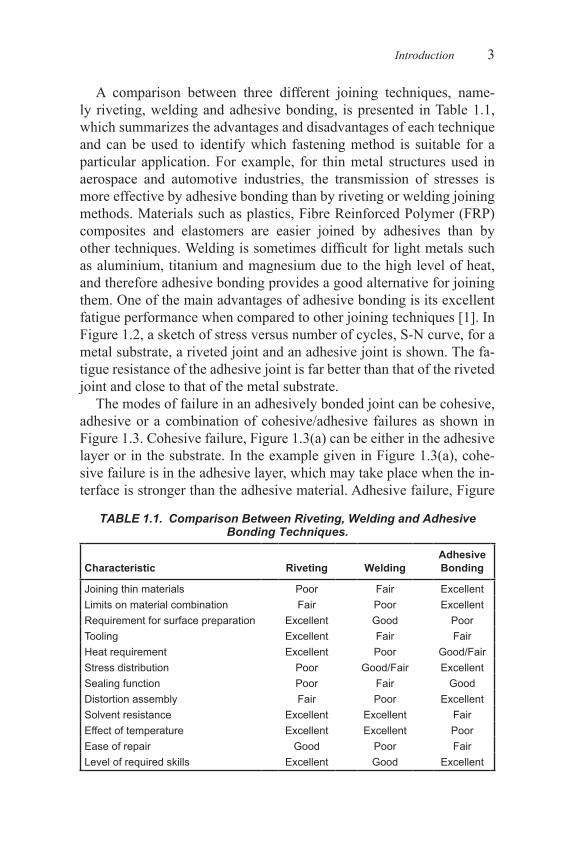
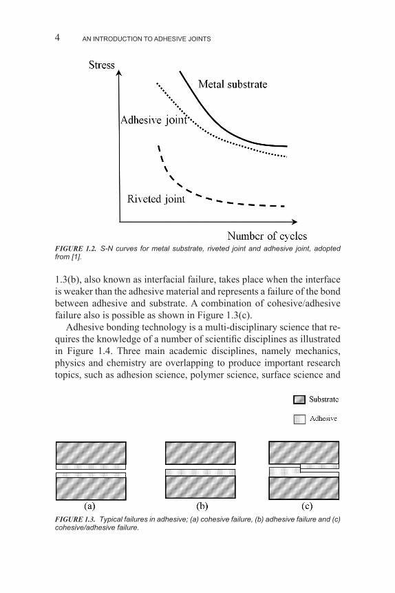
A comparison between three different joining techniques, name-ly riveting, welding and adhesive bonding, is presented in Table 1.1, which summarizes the advantages and disadvantages of each technique and can be used to identify which fastening method is suitable for a particular application. For example, for thin metal structures used in aerospace and automotive industries, the transmission of stresses is more effective by adhesive bonding than by riveting or welding joining methods. Materials such as plastics, Fibre Reinforced Polymer (FRP) composites and elastomers are easier joined by adhesives than by othertechniques.Weldingissometimesdifficultforlightmetalssuchas aluminium, titanium and magnesium due to the high level of heat, and therefore adhesive bonding provides a good alternative for joining them. One of the main advantages of adhesive bonding is its excellent fatigue performance when compared to other joining techniques [1]. In Figure 1.2, a sketch of stress versus number of cycles, S-N curve, for a metal substrate, a riveted joint and an adhesive joint is shown. The fa-tigue resistance of the adhesive joint is far better than that of the riveted joint and close to that of the metal substrate.

The modes of failure in an adhesively bonded joint can be cohesive, adhesive or a combination of cohesive/adhesive failures as shown in Figure 1.3. Cohesive failure, Figure 1.3(a) can be either in the adhesive layer or in the substrate. In the example given in Figure 1.3(a), cohe-sive failure is in the adhesive layer, which may take place when the in-terface is stronger than the adhesive material. Adhesive failure, Figure

Introduction

TABLE 1.1. Comparison Between Riveting, Welding and Adhesive Bonding Techniques.

Characteristic Riveting WeldingAdhesive Bonding

Joining thin materials Poor Fair ExcellentLimits on material combination Fair Poor ExcellentRequirement for surface preparation Excellent Good PoorTooling Excellent Fair FairHeat requirement Excellent Poor Good/FairStress distribution Poor Good/Fair ExcellentSealing function Poor Fair GoodDistortion assembly Fair Poor ExcellentSolvent resistance Excellent Excellent FairEffect of temperature Excellent Excellent PoorEase of repair Good Poor FairLevel of required skills Excellent Good Excellent

AN INTRODUCTION TO ADHESIVE JOINTS4

1.3(b), also known as interfacial failure, takes place when the interface is weaker than the adhesive material and represents a failure of the bond between adhesive and substrate. A combination of cohesive/adhesive failure also is possible as shown in Figure 1.3(c).

Adhesive bonding technology is a multi-disciplinary science that re-quirestheknowledgeofanumberofscientificdisciplinesasillustratedin Figure 1.4. Three main academic disciplines, namely mechanics, physics and chemistry are overlapping to produce important research topics, such as adhesion science, polymer science, surface science and

FIGURE 1.2. S-N curves for metal substrate, riveted joint and adhesive joint, adopted from [1].

FIGURE 1.3. Typical failures in adhesive; (a) cohesive failure, (b) adhesive failure and (c) cohesive/adhesive failure.

5

joint design. This book concentrates on the mechanics aspect of adhe-sive jointsandmorespecificallystressanalysis, fractureanddamagemechanics, thermal, diffusion and coupled analyses using Finite Ele-ment Analysis (FEA) technique.

1.2. A BRIEF HISTORY OF ADHESIVE BONDING

As an Egyptian, I am proud to say that ancient Egyptians were among the early humans in the ancient ages who made use of adhesives. In the tomb of Rekhmara in Tibah, which dates to 1475 B.C., animal glues were used in a wall carving. In the tomb of Tut-an-khamun discovered in 1922 in the Valley of the Kings, a glue tablet was found. Surprisingly, the glue’s properties were found to be identical to those at the time of the archaeological investigations indicating that adhesives have not been further developed since the time of ancient Egyptians. Egyptians used glues in many applications including fastening gold leaf to plaster, fastening wood, sealing and repairing alabaster jars, compound bow and as a binder in paints and pigments.

Although I have started with ancient Egyptians, the history of adhe-

A Brief History of Adhesive Bonding

FIGURE 1.4. Multi-disciplinary aspects of adhesive bonding technology.

AN INTRODUCTION TO ADHESIVE JOINTS6

sivesismucholderthanthat.Itisverydifficultindeedtotracetheexactstarting date for the use of adhesives. It might have been started at the same time as the existence of human being. Archaeological evidence suggests that humans have used adhesives for thousands of years, dating back approximately 200,000 B.C. In Koenigsaue in the Harz Mountains in Germany in 1963, residues of adhesives were found on Neanderthal toolsdatedtoapproximately80,000B.C. Other Neanderthal tools dated to 40,000 B.C. have been found in Umm el Tiel in Syria. Adhesives used bymodernhumanshavebeendated to8,000B.C. Statues discovered in Babylonian temples contain glues and have been dated to 4,000 B.C. The Sumerians in 3000 B.C. used glue produced from animal skins and the Mesopotamians in 4000 B.C. used asphalt. In 1991, a discovery re-vealed adhesives were used to bond components of weapons from the Late Neolithic period dated in 3,300 B.C. During the period between 2000 B.C. and 1600 B.C., ancient Greeks used glues in the famous leg-endofDaedalusandIcarus.Thefirstbondingofstructuralmetalprob-ably was done by the ancient Greek sculptor and architect Theodorus of Samos (from the Greek island of Samos) and is dated to 530 B.C.

In the middle ages, immediately after the decline of Greece and Rome empire, very few records documenting the use of adhesives can be found. It is very likely that adhesives were in use during several cen-turies. The use of adhesives restarted in the 16th century for inlaying workandfurtherinthe17thcenturyforveneering.Inthe18thcentury,adhesives were used in the production of furniture. In 1690, the produc-tion and practical manufacturing of glues started in the Netherlands and movedtoEnglandin1700.Thefirstpatentrelatedtoglue,titled“akindofgluecalledfishglue”,waspublishedinBritainin1754,followedbyother patents related to animal glues during the next few hundred years. During this period, animal and vegetable glues were used to bond wood and paper products. By the end of the 19th century and the beginning of the 20th century, many publications appeared to share knowledge of glue use, manufacturing and testing. Advances were noticeable in many issues including glue production on industrial scale, importance of quality control and testing of adhesive products. By around 1920, the use of adhesives in the manufacturing of aircraft and automobile has been started. The adhesives available at that time were of nature origin [2],namelyanimalglue,fishglue,liquidglueoranimalglueinliquid,marine glue made from indiarubber, naphtha and shellac, casein glue, waterproofglue,vegetableglue,flexibleglue (modifiedanimalglue)and albumen glues.

7

AlexanderParkes introducedcelluloid in1862and started thede-velopmentofsyntheticpolymers,whichhadasignificanteffectonthehistoryofadhesives.In1872,BaeyerhasusedPhenol-formaldehydestoproduceresinsforthefirsttime,followedin1905byLeoBaekeland,whointroducedacommercialproductofasyntheticresincalled“Bake-lite.”In1930,acommercialproductofphenolicresinthatcanbeusedin the manufacturing of polywood was made available. Later on, pheno-lic adhesives were developed in water emulsions and dry powders. The history of the development of Phenol-formaldehydes is summarized in Table1.2[3].In1918,HansJohnproposedtheuseofUrea-formalde-hyde as adhesives. The developments of polyvinyl acetate, polyvinyl chloride and acrylic adhesives took place around 1912 by synthesise and polymerise vinyl acetate and vinyl chloride monomers. Acrylic polymers formed the basis of anaerobics, ultraviolet hardening and two part toughened adhesives. In 1937, Otto Bayer published a patent on isocyanate polyaddition process and developed Polyurethane polymers. Polyurethane adhesives have been used for bonding glass, wood, com-posite, rubber and leather. In 1936, Pierre Castan has introduced epoxy resins, which can be considered as one of the most important product inthehistoryofadhesives[4].Heproducedthefirstsynthesisedepoxyresins. In 1939, Greenlee produced epoxy resins using epichlorhydrin and bispenol A. In 1946, Swiss Industries Fair developed four electrical casting resins for commercial exploitation of epoxy adhesive. Due to their versatility, good mechanical properties and ease of use, epoxy ad-hesives are nowadays used in many industries including aerospace, au-tomotive, electronics and construction. They have high shear strength, but low toughness and peel stress. In order to improve their properties, the use of additives has been proposed. In 1970, butadiene-based rubber modifiersfromGoodrichwasintroducedtoimprovepeel,impactandfatigue resistance.

A Brief History of Adhesive Bonding

TABLE 1.2. Historical Development of Adhesives [3].

Year of Availability Adhesive Type

1910 Phenol-formaldehyde1930 Urea-formaldehyde1940 Nitrile-phenolic, vinyl-phenolic, acrylic, polyurethane1950 Epoxies, cyanoacrylates, anaerobics1960 Polyimide, polybenzimidazole, polyquinoxaline1970 Second-generation acrylic

AN INTRODUCTION TO ADHESIVE JOINTS8

1.3. CLASSIFICATION OF ADHESIVES

Adhesivesmaybeclassifiedinmanydifferentways.Theclassifica-tion of adhesives is quite important for the selection of a proper adhe-sive for a certain application. Today, a large number of adhesive types is available for engineers. This makes the selection of a proper adhesive quiteadifficulttask.Thecommonclassificationsusedintheindustryare by: (1) function, (2) chemical composition, (3) method of reaction, (4) physical form, (5) cost and (6) end use. Table 1.3 summarized the different ways to classify adhesives.

1.3.1.  Classification by Function

Adhesivesareclassifiedbyfunctionasstructuralandnon-structural.Structural adhesives are materials with high strength, which bond struc-tures and resist loads during the service life and in the designed operat-ing environments. Non-structural adhesives bond lightweight materials in place and are not subjected to high external loads. They are used for temporary short term fastening and as a secondary fastener in a hy-brid (e.g. bonded/bolted) joint. Examples of non-structural adhesives include hot meld and water emulsion adhesives.

TABLE 1.3. Classification of Adhesives.

Classification

Function StructuralNon-structural

Chemical composition

ThermosettingThermoplasticElastomeric

Hybrid

Method of reaction

Chemical reactionLoss of solventLoss of water

Cooling from melting

Physical formSolid

100% solid paste and liquid100% solid paste and liquid with solvent to reduce viscosity

Cost Including labor, equipments, curing time, loss due to defective joints

End useSubstrate typeEnvironments

9

1.3.2.  Classification by Chemical Composition

Adhesivesareclassifiedbychemicalcompositionasthermosetting,thermoplastic, elastomeric or combination of them (hybrid). Thermo-setting adhesives cannot be heated and softened after initial cure that takes place by an irreversible chemical reaction at room or elevated temperature. Examples of thermosetting adhesives are epoxy and ure-thane. Thermoplastic adhesives are materials that do not cure or heated. They are solid polymers that melt when heated. After applied to the substrate, the adhesive hardens by cooling. Examples of thermoplastic adhesives are hot-melt adhesives used in packaging. Elastomeric adhe-sives are made from polymeric resins having high degree of elongation and compression. They are hyper-elastic materials that return rapidly to their initial dimensions after the removal of the applied load. Hy-brid adhesives are made by combining thermoplastic, thermosetting or elastomeric resins. This combination makes use of the best properties of each resin. In general, if high temperature rigid resins are combined withflexibletoughelastomers,improvedpeelstrengthandenergyab-sorption can be obtained. Recent development in hybrid adhesive sys-tems resulted in improved peel strength and toughness of thermosetting resins without any reduction in their high temperature properties.

1.3.3.  Classification by Method of Reaction

Adhesivesareclassifiedbymethodofreactionaschemicalreaction,loss of solvent, loss of water and cooling from melting. They may so-lidify by losing solvent or hardening due to heat or chemical reaction. Adhesivesthathardenbychemicalreactionmaybefurtherclassifiedaccording to the type or the use: (1) two parts systems, (2) single part cured via catalyst or hardener, (3) moisture cured, (4) radiation cured such as light, ultraviolet and electron beam, (5) catalyzed by substrates and (6) in solid form such as tape, film and powder.Adhesives thathardenbylossofsolventorwaterareclassifiedas:(1)contact,(2)pres-sure sensitive, (3) reactivatable and (4) resinous. Adhesives that harden bycoolingfrommeltingareclassifiedas:(1)hotmeltand(2)hotmeltpressure sensitive.

1.3.4.  Classification by Physical Form

Adhesives are available in many physical forms and may be clas-

Classification of Adhesives

AN INTRODUCTION TO ADHESIVE JOINTS10

sifiedasliquidorpastemultiplepartsolvent-less,liquidorpasteonepart solvent-less, liquid one part solution and solid including powder, tape,film,etc.Sometypesofadhesivesareavailableinmanyforms,e.g.epoxyadhesive.Asimplerclassificationofadhesivesbyphysicalformwouldbesolidandliquid.Solidadhesivescanbefurtherclassifiedas(1)film,(2)tape,(3)solidpowders,(4)solvedandprimersand(5)hot melt. Liquid adhesives are either pure 100% solid paste and liquid or 100% solid paste and liquid with solvent to reduce viscosity. The firsttypecanbefurtherclassifiedas(1)onecomponentcuredbyheat,surface or anaerobic catalysts, or ultraviolet light or radiation and (2) two components cured at room temperature or heat. The second type is classifiedas(1)solvent-basedcontact,(2)water-basedand(3)pressuresensitive.

1.3.5.  Classification by Cost

Cost plays an important role in the selection of an adhesive; there-fore,itmightbeusedasamethodofclassificationeveninanindirectway. The cost of using adhesives is not just the price of adhesive mate-rials, but it should include other costs that are necessary to produce an adhesive joint. Thus, costs of labor, equipment, curing time, loss due to defective joints should be considered. In analyzing the real cost of an adhesive joint, the following parameters should be considered: (1) efficiencyofbonding,(2)easeofapplicationandrequirementofequip-ment,suchasjigs,ovens,pressersandfixtures,(3)totalprocessingtimefor preparation of substrates, assembly, drying and curing, (4) cost of labour, (5) waste of adhesives and (6) rejected or defected joints.

1.3.6.  Classification by End Use

Adhesivesareclassifiedbyendused,suchassubstratetypethatwillbe jointed and environments for which they are suited. The substrate type can be, for instance, metal, composite, wood, etc. The environment classificationincludeacid-resistant,heat-resistantandweather-ablead-hesives.

1.4. APPLICATIONS OF ADHESIVE BONDING

Adhesive bonding has been successfully used in many industrial ap-plications.Inordertochooseanadhesivesystemforaspecificapplica-

11

tion many factors should be considered. Strength, fatigue resistance, durability and expected lifetime are examples of such factors. The clas-sificationspresentedintheprevioussectionwouldbeveryhelpfultoevaluate the suitability of an adhesive system for a certain application. In industrial applications, structural reactive adhesives provide high strength, durability and temperature resistance. In the following sec-tions, some important industrial applications are reviewed.

1.4.1.  Aerospace

In 1970, the U.S. Air Force funded the project Primarily Adhesive Bonded Structures Technology (PABST), in which aluminium aircraft structures were bonded with adhesives. The aim of this project was to produce repeatable and reliable bonding by determining the optimum joint design, the best surface treatment procedures and procedures for storage and application of adhesives. A summary of the type of adhesives used to bond different aircraft components is given in Table 1.4. Due to the importance of light weight in aircraft, adhesive systems usually are supplied as syntactics, which are types of foam materials. In general, the types of adhesives used for aircraft structures are one-component liquidsandpastacuredbyheat,two-componentliquidsandpasts,filmsandpressuresensitive.Epoxypastaandfilm,whicharecuredinheatedpresses, are used to bond honeycomb panels and to bond skins to hon-eycomb. Honeycomb panels are fabricated from aluminium sheets in a sandwich structure bonded to a honeycomb core. In the construction of aileron at the trailing edge of the wing, laminate structures are made of epoxy graphite plies. Adhesives are used not only in bonding criti-cal aircraft components such as fuselage and fuel tanks, but also to a great extent in bonding and sealing interior components, such as panels, seats, tray tables, overhead bins, galleys, toilets, etc.

Applications of Adhesive Bonding

TABLE 1.4. The Use of Adhesive in Aircraft Structures [5].

Bonded Structures Adhesive Type

Metal honeycombs and skins EpoxyMetal honeycombs and skins for high temperature situations Nitrile phenolicInterior plastics Acrylic, Pressure

sensitive adhesivesSealing interior plastics SiliconePlastics and composites Polyurethane

AN INTRODUCTION TO ADHESIVE JOINTS12

1.4.2.  Automotive

During the last few decades, the application of adhesive bonding to automotive industry has been significantly increased due to the newrequirements of using thin panels of metals, such as steel, aluminium and magnesium, and the increased in the use of plastic. Adhesives are used in many of the essential components of a vehicle, such as the powertrain, body, trim, electrical system and brakes. A summary of the applications and adhesive types used for each component is given in Table 1.5. There are many applications for adhesives and sealants in

TABLE 1.5. The Use of Adhesives in Automotive [5].

Component Applications Adhesive/Sealant Type

Powertrain

Threadlocking AnaerobicsOil pan gasketing, Rocker

cover gasketSilicones

Oil filter assembly Plastisols, cyanoacrylatesClutch facings Phenolics

Body

Hem flange bonding Plastisols, epoxies, polyurethaneBody-in-white sealing Plastisols, rubbers, Polyvinyl

ChlorideRoof bow joints Rubber

Anti-flutter stiffeners SBR, polybutadienePlastic panel bonds Epoxies, polyurethane

Bumper bonding Reactive acrylics, polyurethaneCavity sealants Expandable polyurethane

Trim

Labels, decals Acrylic pressure sensitiveRear parcel shelves Hot melts, reactive hot melt poly-

urethanesSun visors, Floor insulation Hot melts

Mirrors SiliconesUpholstered seats, Headliner Hot melts, reactive hot melt poly-

urethanesDashboard Polyurethane, hot melts

Carpet bonding Hot melts, pressure sensitiveWindshield bonding Polyurethane

Electrical systems

Headlight units Epoxies, ultraviolet acrylicsRearlight units Silicones, hot melts

Spark plug seals SiliconesMotor bonding Anaerobics, reactive acrylics,

ultraviolet acrylics

Brakes Disk pad bonding Phenolics

57

CHAPTER 3

Finite Element Analysis 

3.1. INTRODUCTION

THIS chapter is intended to provide a basic background for the Finite Element Analysis (FEA). It concentrates on topics that are required

for the analysis of adhesively bonded joints, which will be presented in later chapters. A brief history of FEA in general and of ANSYS pack-age in particular is presented. As the analysis of bonded joints will be in two-dimensional space, the theoretical aspects of two-dimensional solidstructuralelementsarebrieflyreviewed.Specificmodellingtech-niques, which are directly related to FEA of adhesively bonded joints, such as geometric and material non-linearities, modelling of singulari-ties and cracks, extracting fracture mechanics parameters from FEA re-sults and modelling of Cohesive Zone Model, are summarized. Because heat transfer and diffusion problems will be presented in other chapters, the formulation of two-dimensional heat transfer conduction element is reviewed. FE formulation for steady state and transient heat transfer anddiffusionanalysesisbrieflypresented.Furthermore,ANSYSpara-metric design language, which is required for modelling and analysing adhesively bonded joints in later chapters, is reviewed.

3.2. A BRIEF HISTORY OF FEA

Although originally developed for stress analysis in complex air-framestructures,FEAcurrentlyisapplicabletothebroadfieldofcon-tinuum mechanics and many other disciplines. FEA is receiving much attentioninacademiaandindustriesbecauseofitsdiversity,flexibility

FINITE ELEMENT ANALYSIS58

and ability to provide approximated numerical solutions to a wide range of engineering applications. The ideas of FEA are shared between three different specialists, namely an applied mathematician, a physicist and an engineer. At a certain point in the FEA history, each of these three specialists has independently developed the essential ideas of FEA for different reasons. The applied mathematicians were interested in solv-ingboundaryvalueproblemsofcontinuummechanicsbyfindingap-proximate upper and lower bounds for eigenvalues. The physicists were concerned with also solving continuum problems by obtaining piece-wise approximate functions, whereas the engineers were interested in solvingcomplexproblemsinaerospacestructuresandfindingthestiff-ness of shell structures reinforced by ribs and spars.

In the applied mathematics literature in 1943, Courant [34] used for the first time piecewise continuous functions defined over triangularelements to study Saint-Venant torsion problem. In 1959, Greenstadt [35] presented an approach in which a continuous problem was reduced to a discrete problem. He used a discretization approach involving cells instead of points so the solution domain was divided into sets of sub-domains. Since the late 1960s, the popularity of FEA has grown and applied mathematicians increased their studies in different aspects, in-cluding estimation of discretization error, rate of convergence and sta-bility of different types of FEA formulation.

During almost the same period mentioned above, physicists also were busy with their FEA ideas. In 1947, Prager and Synge [36] pub-lished their development of the hyper-circle method, which originally was developed in conjunction with the classical theory of elasticity. Synge [37] demonstrated the hyper-circle method can be applied to continuum problems in a way similar to FEA.TheengineeringcommunityhasforthefirsttimeadoptedFEAideas

in the 1930s, when a structural engineer analyzed a truss problem by solving components of stress and defection. This was done by consid-ering the truss as an assembly of rods whose elastic behavior was well known. Then, by combining the individual elements, applying equilib-rium equations and solving the resulting system of equations, unknown forces and defection would be obtained for the whole structure. In order toapplythisconcepttoanelasticcontinuumstructure,Hrenikoff[38],in 1941, divided the continua into beam elements interconnected at a finitenumberofnodes.Usingthisconcept, theproblemcanbesolvedin a way similar to that used for the truss. Further development of Hre-nikoff’s idea was reported by McHenry [39] in 1943, Kron [40,41] in

59

1944 and Newmark [42] in 1949. Starting from 1954 to around 1960, Argyris [43–46] presented techniques to deal with linear structural analysis and efficient solution for automatic digital computation. In1956,Turneretal[47]havepresentedthefirstsolutionofplanestresscontinuum problems using triangular and elasticity theory. They have introducedforthefirsttimethedirectstiffnessmethod,whichwasusedto determine thefinite element properties.The term “FiniteElementMethod”(FEM)wasfirstlyusedbyClough[48] in1960forsolvingplaneelasticityproblems.Theterm“FiniteElementAnalysis”(FEA)can be considered as the practical application of FEM. In 1965, Zien-kiewiczandCheung[49]reportedthatFEAwasapplicabletoallfieldsthat can be treated with variational form principles. Since the 1960s, the interest in FEA among engineers and scientists has grown quickly. A tremendous amount of technical papers has been published; a large number of conferences have been organized; and numerous books on the topic have appeared. A simple search in Google search engine on thephrase“FiniteElement”resultsinapproximately13,200,000resultsandasearchinthewebofscienceonthetopic“FiniteElement”resultsin approximately 423,231 articles.

3.3. A BRIEF HISTORY OF ANSYS PACKAGE

In 1970, Swanson Analysis Systems Inc. (SASI) founded ANSYS. Oneyearlater,thefirstversionofANSYSsoftware,ANSYS2.0,wasreleased. Geometric non-linearities and thermo-electric elements have beenincludedinANSYSsince1975.In1981,SASIusedthefirstwork-stationasanalternativetomainframes.Fewyearslater,in1983,electro-magnetic analysis was introduced and the next version of ANSYS with electromagnetic capabilitieswas released. In 1985, SASI has startedto offer online help and ANSYS software has incorporated parametric analysis and structural optimization. Color graphics and layered com-positesolidelementswereintroducedin1987.In1991,generalpurposeCFD solver for unstructured grids and TGrid tetrahedral mesher were released. In 1993, a new ANSYS software, namely Machine Design’s best Finite Element Analysis software for workstation, was released. In 1994, SASI renamed ANSYS, Inc. In 1996, ANSYS became a public company listed on the National Association of Securities Dealers Auto-mated Quotations, NASDAQ (ANSS), and released DesignSpace with ANSYS workbench environment, ANSYS and LS-DYNA for crash and drop test simulations and commercial CFD with parallel processing.

A Brief History of ANSYS Package

FINITE ELEMENT ANALYSIS60

Automaticcontactdetectionforassemblieswasintroducedin1998.Ayear later, ANSYS acquired Centric Engineering Systems Inc., adding multi-physics modelling and high-performance processing capabilities. Furthermore, in 2000, ANSYS acquired the meshing and post-process-ing tools of ICEM CFD Engineering and, in 2001, the designXplorer tool for post-processing of CADOE S.A. Semi-automated easy-to-use moving deformed mesh, multi-domain material phase model for un-structured mesh and commercial k-turbulence model for unstructured meshwasaddedin2001.In2003(ANSYS7.1and8.0),ANSYSac-quired CFX and released automated dynamic mesh capability and fea-ture based mesh adaption for CFD. Solving hundred million degrees of freedommadepossiblein2004.In2005,theseamlesslycoupledfluid-structure interaction (FSI) was introduced, and ANSYS acquired Cen-tury Dynamics Inc. and Harvard Thermal Inc. adding explicit dynamics and electronics cooling analysis tools. In 2006, ANSYS acquired Fluent Inc. and itsfluiddynamics tools. Integrated rigid andflexiblemulti-bodydynamicswaslaunchedin2007.In2008,ANSYSacquiredAn-soft Corporation introducing high performance electronics software. In 2009 (ANSYS 12.0), ANSYS released the next-generation of ANSYS workbench and in 2010 ANSYS celebrated its 40th anniversary.

Nowadays, ANSYS becomes a comprehensive Finite Element soft-ware that contains more than 100,000 lines of codes. It has the capa-bilities to perform a wide range of analysis disciplines, such as static, dynamic, heat transfer electro-magnetic, etc. ANSYS is used in many engineering applications, including aerospace, mechanical, civil, ma-rine, electronic and nuclear. ANSYS Graphical User Interface (GUI) has been evolved during the years and its current form consists of a graphic window, a main menu, an utility menu and a toolbar.

3.4.  STRUCTURAL MECHANICS PROBLEMS

3.4.1.  Two-dimensional Solid Element

3.4.1.1. Linear Elements

In displacement formulation FEA, for two-dimensional solid ele-ment, the degrees of freedom are the displacements in two directions, e.g. in the x and y directions if Cartesian coordinates are considered. Thefirststepinformulatingtwo-dimensionalelementistoexpressthefunctions of degrees of freedom in terms of their nodal values. In other

61Structural Mechanics Problems

(3.1)

(3.2)

(3.3)

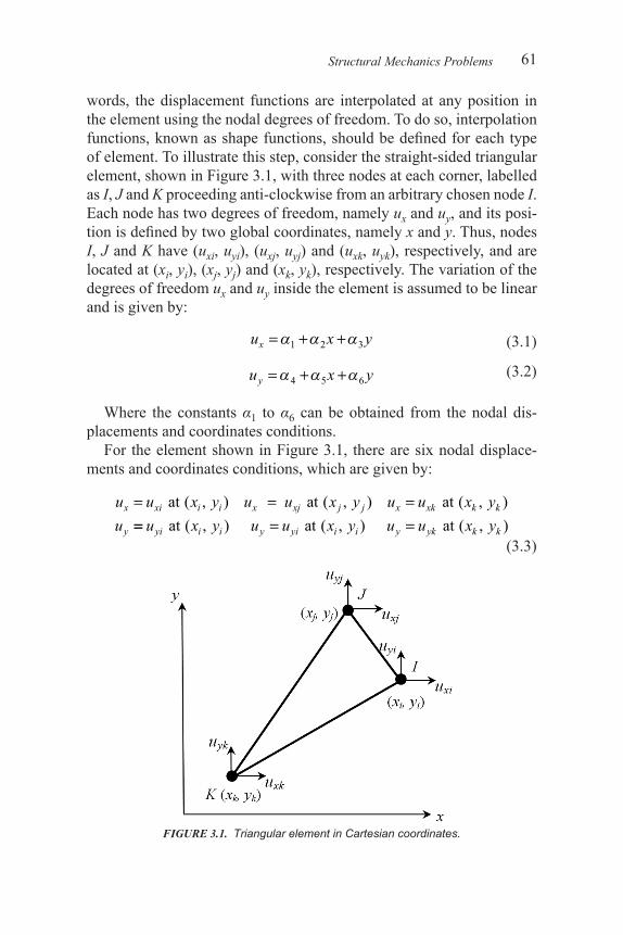
FIGURE 3.1. Triangular element in Cartesian coordinates.

words, the displacement functions are interpolated at any position in the element using the nodal degrees of freedom. To do so, interpolation functions,knownasshapefunctions,shouldbedefinedforeachtypeof element. To illustrate this step, consider the straight-sided triangular element, shown in Figure 3.1, with three nodes at each corner, labelled as I, J and K proceeding anti-clockwise from an arbitrary chosen node I. Each node has two degrees of freedom, namely ux and uy, and its posi-tionisdefinedbytwoglobalcoordinates,namelyx and y. Thus, nodes I, J and K have (uxi, uyi), (uxj, uyj) and (uxk, uyk), respectively, and are located at (xi, yi), (xj, yj) and (xk, yk), respectively. The variation of the degrees of freedom ux and uy inside the element is assumed to be linear and is given by:

u x yx = + +α α α1 2 3

u x yy = + +α α α4 5 6

Where the constants α1 to α6 can be obtained from the nodal dis-placements and coordinates conditions.

For the element shown in Figure 3.1, there are six nodal displace-ments and coordinates conditions, which are given by:

u u x y u u x y u u x yu

x xi i i x xj j j x xk k k

y

= = = at at at ( , ) ( , ) ( , )== = =u x y u u x y u u x yyi i i y yi i i y yk k k at at at ( , ) ( , ) ( , )

137

CHAPTER 5

Stress Analysis

5.1. INTRODUCTION

AFTER constructing the FE models of the bonded joints in Chapter 4, stress analysis for these joints is carried out in this chapter. In all

analyses considered in this chapter, non-linear elastic plastic stress-strainbehavior isdefined for theadhesivematerial.The substratesare chosen to be either metallic (Aluminium or Steel) or CRFP com-posite unidirectional or multidirectional laminates. As most joints show high rotation due to the offset of loading, large deformation should be activated in the analysis. Therefore, both material nonlin-earity (see section 3.4.2.2 in Chapter 3) and geometric nonlinearity (see section 3.4.2.1) should be taken into account during the solution of the FEA equations. The load is applied in different sub-steps and the solution is obtained incrementally as explained in section 3.4.2.3. Four joints are analyzed in this chapter, namely SLJ, DLJ, LSJ and BJ, which are the four un-cracked joints considered in Chapter 4. Forstressanalysisofeach joint, twofilesarecreatedandsuppliedwiththisbook.Thefirstfilehasthenameformat‘jointname_Smo-del.inp’andcontainsthedefinitionofmaterialproperties,geometricparameters, keypoints, meshing, etc., as explained in Chapter 4. The secondfile,whichcallsthefirstfilewith/INPUTcommand,appliesloads and boundary conditions, and performs the stress analysis. This stressanalysisfilehasthenameformat‘jointname_stress_analysis.inp’.Itshouldbenotedthatbothfilesshouldbeinthesamedirec-torysothatANSYScanfindthefirstfilewhenitisimportedinthesecondfile.

STRESS ANALYSIS138

5.2. STRESS ANALYSIS USING ANSYS

5.2.1.  Single Lap Joint—Metallic substrates

ForSLJ,thefile‘SLJ_Smodel.inp’isimportedtothestressanalysisfile,‘SLJ_stress_analysis.inp’beforeapplyingboundaryconditionsandloads,andsolvingtheproblem.Then,wedefineoneadditionalparam-eter, namely the applied force in Newton, which is acting at both ends of the substrates and distributed over the thickness and the width of the substrates as shown in Figure 5.1. ANSYS commands for these two steps are:

/SOLU ! Enter solution processorKSEL,s,loc,x,0 ! Select keypoints at x=0, left edge of the lower

substrateKSEL,r,loc,y,0 ! Select from previous selection keypoints at

y=0 (only one keypoint is selected)DK,all,all ! Constrain all DOF at selected keypointKSEL,s,loc,x,2*lt-lo ! Select keypoints at x=2lt-lo, right edge of the

upper substrateKSEL,r,loc,y,tadh+tadv ! Select from previous selection keypoints at y=

tadh+tadv (only one keypoint is selected)DK,all,uy ! Constrain displacement in the y direction at

selected keypoint

/INPUT,SLJ_Smodel,inp ! Import SLJ modelft=200 ! DefinetotalappliedloadinN

All commands related to applying boundary conditions and load should be issued in the solution processor, which can be entered through the command /SOLU. The SLJ is modelled assuming simply supported boundary conditions by constraining one keypoint (and node) at the left hand side of the lower substrate in the x and y directions (all DOF) and one keypoint at the right hand side of the upper substrate in the y directions (only uy). This is done in ANSYS by selecting the relevant keypoint using KSEL command without the need to know the number of each keypoint. ANSYS commands for applying boundary conditions are:

/TITLE,Single Lap Joint - Stress Analysis ! Defineatitlefortheanalysis

Furtheratitleisdefined,using/TITLEcommand,as:

139

Alternatively,keypointsmaybeexplicitlydefinedbytheirnumbers.In order to include the geometric nonlinearity, the command NLGEOM isissuedtoswitchontheeffectoflargedeflection.ThecommandLN-SRCH also is issued to activate a line search to be used with Newton-Raphson iteration method. This is useful for the convergence of the nonlinear solution, especially for bonded joints where both geometric and material nonlinearities are present. ANSYS commands for these two steps are:

Stress Analysis Using ANSYS

FIGURE 5.1. SLJ mesh, applied pressure and boundary conditions.

NLGEOM,on ! Include geometric nonlinearity (large deformation) in the analysis

LNSRCH,on ! Activate a line search for Newton-Raphson

TIME,1 ! Set time for load step to 1KBC,0 ! Apply ramped loading within this load step

For non-linear analysis, the load is applied in steps so that the solu-tion is performed in sub-steps. If only one load step is applied as in our case, the load step starts at time 0 and ends at time 1. The load varies linearly as a function of time as shown in Figure 5.2. The solution then will be obtained at different time sub-steps, i.e. different load sub-steps. To specify the time at the end of a load step in ANSYS, the command TIME is used. The linear variation of loading (ramped) is applied using the command KBC. Although the default of the command is ramped loading, it is given herein for completeness:

FIGURE 5.2. Load as a function of time for nonlinear analysis.

STRESS ANALYSIS140

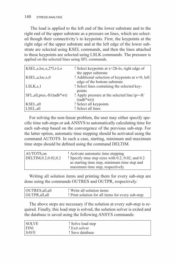
The load is applied to the left end of the lower substrate and to the right end of the upper substrate as a pressure on lines, which are select-ed though their connectivity’s to keypoints. First, the keypoints at the right edge of the upper substrate and at the left edge of the lower sub-strate are selected using KSEL commands, and then the lines attached to these keypoints are selected using LSLK commands. The pressure is applied on the selected lines using SFL commands.

KSEL,s,loc,x,2*Lt-Lo ! Select keypoints at x=2lt-lo, right edge of the upper substrate

KSEL,a,loc,x,0 ! Additional selection of keypoints at x=0, left edge of the bottom substrate

LSLK,s,1 ! Select lines containing the selected key-points

SFL,all,pres,-ft/(tadh*wt) ! Apply pressure at the selected line (p=-ft/(tadh*wt))

KSEL,all ! Select all keypointsLSEL,all ! Select all lines

AUTOTS,on ! Activate automatic time steppingDELTIM,0.2,0.02,0.2 ! Specify time step sizes with 0.2, 0.02, and 0.2

as starting time step, minimum time step and maximum time step, respectively

OUTRES,all,all ! Write all solution itemsOUTPR,all,all ! Print solution for all items for every sub-step

SOLVE ! Solve load stepFINI ! Exit solverSAVE ! Save database

For solving the non-linear problem, the user may either specify spe-cifictimesub-stepsoraskANSYStoautomaticallycalculatingtimeforeach sub-step based on the convergence of the previous sub-step. For the latter option, automatic time stepping should be activated using the command AUTOTS. In such a case, starting, minimum and maximum timestepsshouldbedefinedusingthecommandDELTIM.

Writing all solution items and printing them for every sub-step are done using the commands OUTRES and OUTPR, respectively:

The above steps are necessary if the solution at every sub-step is re-quired. Finally, this load step is solved, the solution solver is exited and the database is saved using the following ANSYS commands:

141Stress Analysis Using ANSYS

/POST1 ! Enter post-processor/DSCALE,1,AUTO ! Scale displacements automaticallyPLDISP,1 ! Display the deformed structure

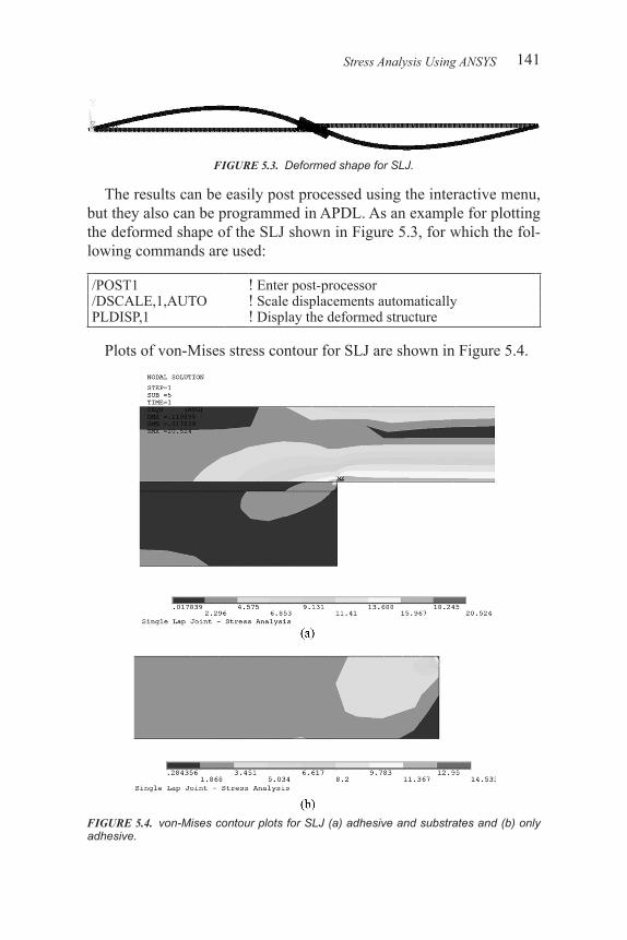
The results can be easily post processed using the interactive menu, but they also can be programmed in APDL. As an example for plotting the deformed shape of the SLJ shown in Figure 5.3, for which the fol-lowing commands are used:

Plots of von-Mises stress contour for SLJ are shown in Figure 5.4.

FIGURE 5.3. Deformed shape for SLJ.

FIGURE 5.4. von-Mises contour plots for SLJ (a) adhesive and substrates and (b) only adhesive.

STRESS ANALYSIS142

5.2.2.  Double Lap Joint—CFRP Composite Substrates

The input file for DLJ stress analysis, ‘DLJ_stress_analysis.inp’,startswithcallingthefilecontainingtheDLJmodel,‘DLJ_Smodel,inp’,developed in Chapter 4, using /INPUT command:

/INPUT,DLJ_Smodel,inp ! Import DLJ model

ft=1200 ! DefinetotalappliedloadinN

KSEL,s,loc,x,0 ! Select keypoints at x=0, left edge of the middle substrate

DK,all,all,0,,1 ! Constrain all DOF at all selected keypoints

KSEL,s,loc,y,0 ! Select keypoints at y=0, symmetric lineDK,all,uy,0,,1 ! Constrain uy at all selected keypoints, symmetric

boundary conditions

KSEL,s,loc,x,l1+l2-lo ! Select keypoints at right edge of the upper substrate

KSEL,r,loc,y,tadh/2+tadv ! Select from previous selection keypoints at y= tadh+tadv (only one keypoint is selected)

DK,all,uy ! Constrain displacement in the y direction at selected keypoint

FIGURE 5.5. DLJ mesh, applied pressure and boundary conditions.

TheappliedloadinNewton’sisdefinedasaparameter:

After entering the solution processor, boundary conditions can be ap-plied. A summary of boundary conditions and applied load is illustrated inFigure5.5.ThemiddlesubstrateoftheDLJisfixedatthelefthandside:

Due to symmetry the mid-plane of the middle substrate is constrained in the y-direction:

One node is constrained in the y-direction at the right edge of the upper substrate by constraining one keypoint using KSEL command:

143Stress Analysis Using ANSYS

KSEL,s,loc,x,l1+l2-lo ! Select keypoints at right edge of the upper substrate

LSLK,s,1 ! Select lines containing the selected key-points

SFL,all,pres,-ft/(tadh*wt) ! Apply pressure at the selected line (p=-ft/(tadh*wt))

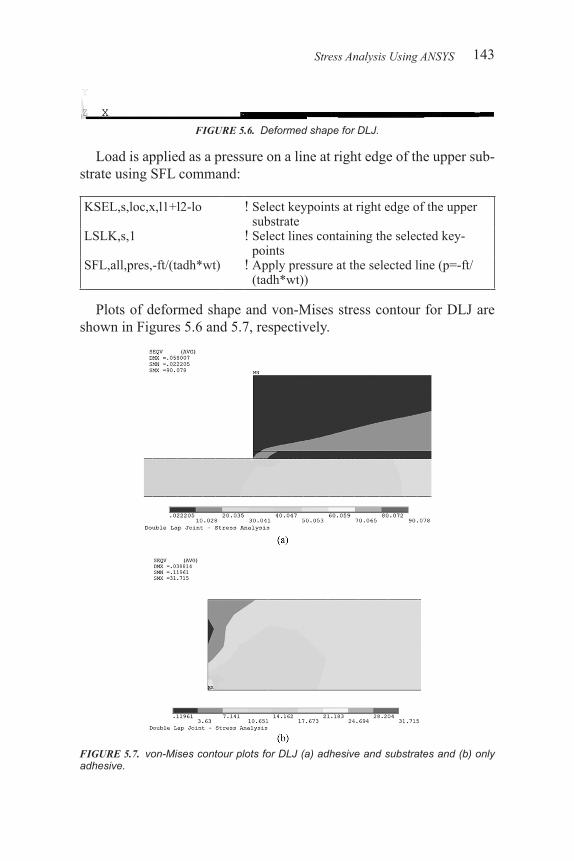
Load is applied as a pressure on a line at right edge of the upper sub-strate using SFL command:

Plots of deformed shape and von-Mises stress contour for DLJ are shown in Figures 5.6 and 5.7, respectively.

FIGURE 5.6. Deformed shape for DLJ.

FIGURE 5.7. von-Mises contour plots for DLJ (a) adhesive and substrates and (b) only adhesive.

STRESS ANALYSIS144

5.2.3 Lap Strap Joint—CFRP Composite Substrates

Similar to the previous two joints, the stress analysis of LSJ is carried outusingtheinputfile‘LSJ_stress_analysis.inp’,whichcallstheLSJmodel developed in Chapter 4:

/INPUT,LSJ_Smodel,inp ! Import LSJ model

ft=1500 ! DefinetotalappliedloadinN

KSEL,s,loc,x,l1+l2 ! Select keypoints at x=l1+l2, right edge of the upper substrate

DK,all,all,0,,1 ! Constrain all DOF at all selected keypoints

KSEL,s,loc,x,0 ! Select keypoints at x=0, left edge of the lower substrate

DK,all,uy,0,,1 ! Constrain uy at all selected keypoints

KSEL,s,loc,x,0 ! Select keypoints at x=0, left edge of the lower substrate

LSLK,s,1 ! Select lines containing the selected keypointsSFL,all,pres,-ft/(tadh*wt) ! Apply pressure at the selected line (p=-ft/

(tadh*wt))

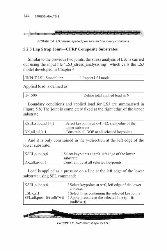
FIGURE 5.8. LSJ mesh, applied pressure and boundary conditions.

Appliedloadisdefinedas:

Boundary conditions and applied load for LSJ are summarised in Figure5.8.Thejointiscompletelyfixedattherightedgeoftheuppersubstrate:

And it is only constrained in the y-direction at the left edge of the lower substrate:

Load is applied as a pressure on a line at the left edge of the lower substrate using SFL command:

FIGURE 5.9. Deformed shape for LSJ.

211

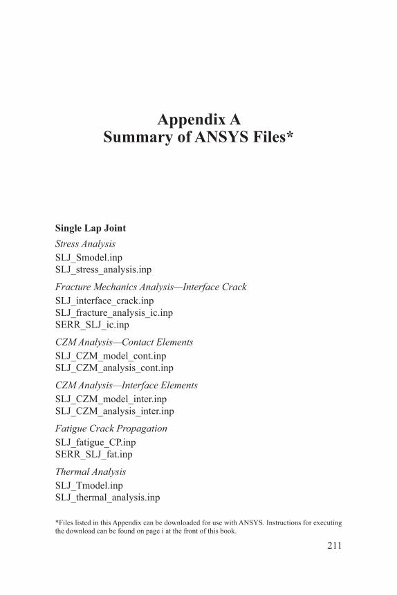
Appendix A Summary of ANSYS Files*

Single Lap JointStress AnalysisSLJ_Smodel.inpSLJ_stress_analysis.inp

Fracture Mechanics Analysis—Interface CrackSLJ_interface_crack.inpSLJ_fracture_analysis_ic.inpSERR_SLJ_ic.inp

CZM Analysis—Contact ElementsSLJ_CZM_model_cont.inpSLJ_CZM_analysis_cont.inp

CZM Analysis—Interface ElementsSLJ_CZM_model_inter.inpSLJ_CZM_analysis_inter.inp

Fatigue Crack PropagationSLJ_fatigue_CP.inpSERR_SLJ_fat.inp

Thermal AnalysisSLJ_Tmodel.inpSLJ_thermal_analysis.inp

*Files listed in this Appendix can be downloaded for use with ANSYS. Instructions for executing the download can be found on page i at the front of this book.

Appendix A212

Coupled Thermal-Stress AnalysisSLJ_Tmodel.inpSLJ_thermal_analysis.inpSLJ_Smodel.inpSLJ_coupled_analysis.inpInterp_mat_SLJ.inpInput_mat_SLJ.inp

Double Lap Joint

Stress AnalysisDLJ_Smodel.inpDLJ_stress_analysis.inp

Fracture Mechanics Analysis—Adhesive CrackDLJ_adhesive_crack.inpDLJ_fracture_analysis_ac.inpSERR_DLJ_ac.inp

Lap Strap Joint/Cracked Lap Shear

Stress AnalysisLSJ_Smodel.inpLSJ_stress_analysis.inp

Fracture Mechanics Analysis—Interface CrackCLS_interface_crack.inpCLS_fracture_analysis_ic.inpSERR_CLS_ic.inp

CZM Analysis—Contact ElementsLSJ_CZM_model_cont.inpLSJ_CZM_analysis_cont.inp

Diffusion AnalysisLSJ_Dmodel.inpLSJ_diffusion_analysis.inp

Coupled Diffusion-Stress AnalysisLSJ_Dmodel.inpLSJ_diffusion_analysis.inp

213

LSJ_Smodel.inpLSJ_coupled_analysis.inpInterp_mat_LSJ.inpInput_mat_LSJ.inp

Butt Joint

Stress AnalysisBJ_Smodel.inpBJ_stress_analysis.inp

Diffusion AnalysisBJ_Dmodel.inpBJ_diffusion_analysis.inp

Coupled Diffusion-Stress AnalysisBJ_Dmodel.inpBJ_diffusion_analysis.inpBJ_Smodel.inpBJ_coupled_analysis.inpInterp_mat_BJ.inpInput_mat_BJ.inp

Double Cantilever Beam 

Fracture Mechanics Analysis—Adhesive CrackDCB_adhesive_crack.inpDCB_fracture_analysis_ac.inpSERR_DCB_ac.inp

CZM Analysis—Contact ElementsDCB_CZM_model_cont.inpDCB_CZM_analysis_cont.inp

CZM Analysis—Interface ElementsDCB_CZM_model_inter.inpDCB_CZM_analysis_inter.inp

Fatigue Crack PropagationDCB_fatigue_CP.inpSERR_DCB_fat.inp

Appendix A

215

Index

Axisymmetric, 100, 114

Butt Joint (BJ), 99, 100, 114, 145, 188, 204

CFRP (Carbon Fibre Reinforced Poly-mer) substrate, 15, 99, 100, 103, 106, 108, 111, 142, 144, 171, 172, 187, 203

Unidirectional laminates, 103, 137, 171

Multi-directional laminates, 103, 104 Cohesive Zone Model (CZM), 27, 57,

79, 83, 99, 149, 157–165 Cracked Lap Strap (CLS), 99, 121

Double Cantilever Beam (DCB), 99, 124, 131, 135, 155, 160, 163, 178

Double Lap Joint (DLJ), 99, 111, 119, 142, 152

Diffusion analysis, 54, 55, 90–92, 100, 107, 114, 115, 183, 186–189, 191, 192, 198, 204

Diffusion equation, 49, 55, 90, 91, Fickian diffusion, 49 Coefficient of diffusion, 90, 91, 107,

108Moisture concentration, 2, 21, 49, 51,

55, 90–92, 100, 187–189, 191, 199–201, 203

Moisture dependent material proper-ties, 191, 192, 198, 199, 204, 205

Fatigue Crack growth rate, 45 Crack propagation, 44, 45, 117,

167–181 Finite Element

Contact, 79, 99, 126–132, 135, 149, 150, 157–161

Interface, 79, 82, 132–136, 149, 150, 160, 162–164

Linear, 60, 64, 66, 76, 77, 133 Quadratic, 65, 66, 72, 135Structural solid, 99, 100 Thermal solid, 100, 107

Heat transferSteady state, 46, 48, 49, 57, 84, 86,

89, 92, 168 Transient, 46, 49, 50, 57, 89, 90, 92,

185

Lap Strap Joint (LSJ), 72, 99, 112, 129, 144, 157, 186, 198

Metallic substrate, 99, 102, 106, 107, 138, 145, 183, 196

Aluminium, 102, 106, 107, 108Steel, 137

Preface216

Non-linearityGeometric, 57, 59, 68, 137, 139, 175 Material, 57, 69, 101, 137, 139, 168

Plane stress, 33, 34, 38, 39, 42, 43, 67, 100

Plane strain, 38, 39, 42, 43, 67, 68, 100, 103, 108, 132, 133, 172,

Plasticity, 21, 28–36

Single Lap Joint (SLJ), 72, 99, 108, 116, 126, 132, 138, 150, 157, 160, 169, 184, 192

StrainEngineering, 22, 23, 25Normal, 21Principal, 25Shear, 24, 25True, 22, 23, 28

Strain Energy Release Rate (SERR), 36, 39, 40, 41, 43–46, 76, 77, 80-82, 128, 149, 150, 153, 167, 168

StressEngineering, 22, 23 Hydrostatic, 27 Interface, 161–165Normal, 21, 22, 24, 26, 27Principal, 24–27, 33 True, 22, 23, 28, 29Ultimate, 101, 102, 194, 195, 197 von-Mises, 27, 33, 141, 143, 144,

147, 197, 198 Yield, 28, 29, 31–35, 101, 194, 195,

200 Stress intensity factor, 36, 38, 39, 41,

74–76

Temperature dependent material proper-ties, 192, 193, 199, 200

Thermal analysis, 100, 105, 107, 110, 184, 188, 192, 197

Traction separation law, 79, 80, 83, 135

Yield criterion, 32–35