FINITE ELEMENT METHOD BASEDSIMULATION, DESIGN, AND RESONANTMODE ANALYSIS OF RADIO FREQUENCYBIRDCAGE COILS USED IN MAGNETIC

RESONANCE IMAGING

a thesis

submitted to the department of electrical and

electronics engineering

and the graduate school of engineering and science

of bilkent university

in partial fulfillment of the requirements

for the degree of

master of science

By

Necip Gurler

August, 2012

I certify that I have read this thesis and that in my opinion it is fully adequate,

in scope and in quality, as a thesis for the degree of Master of Science.

Prof. Dr. Yusuf Ziya Ider(Advisor)

I certify that I have read this thesis and that in my opinion it is fully adequate,

in scope and in quality, as a thesis for the degree of Master of Science.

Prof. Dr. Ergin Atalar

I certify that I have read this thesis and that in my opinion it is fully adequate,

in scope and in quality, as a thesis for the degree of Master of Science.

Prof. Dr. Nevzat Guneri Gencer

Approved for the Graduate School of Engineering and Science:

Prof. Dr. Levent OnuralDirector of the Graduate School

ii

ABSTRACT

FINITE ELEMENT METHOD BASED SIMULATION,DESIGN, AND RESONANT MODE ANALYSIS OFRADIO FREQUENCY BIRDCAGE COILS USED IN

MAGNETIC RESONANCE IMAGING

Necip Gurler

M.S. in Electrical and Electronics Engineering

Supervisor: Prof. Dr. Yusuf Ziya Ider

August, 2012

Radio Frequency (RF) birdcage coils are widely used in Magnetic Resonance

Imaging (MRI) since they can generate very homogeneous RF magnetic field in-

side the coil and have high signal-to-noise ratio (SNR). In practice, designing a

birdcage coil is a time-consuming and difficult task. Calculating the capacitance

value, which is necessary for the coil to resonate at the desired frequency, is the

starting point of the design process. Additionally, it is also important to know

the complete resonance frequency spectrum (or resonant modes) of the birdcage

coil that helps the coil designers to be sure that working mode is far away from

the other modes and so that tuning and matching procedures of the coil can be

done without interfering with the other modes. For this purpose, several studies

have been presented in the literature to calculate the capacitance value and the

resonant modes of the birdcage coil. Among these studies, lumped circuit element

model is the most used technique in capacitance and resonant modes calculations.

However, this method heavily depends on the inductance calculations which are

made under quasi-static assumptions. As a consequence of this assumption, error

in the calculations increases as the frequency increases to a point at which the

wavelengths are comparable with the coil dimensions. Additionally, modeling

the birdcage coil in a 3D simulation environment and making electromagnetic

analysis in the volume of interest is also important in terms of observing the elec-

tromagnetic field distributions inside the coil. In this thesis, we have proposed

three different Finite Element Method (FEM) based simulation methods which

are performed using the developed low-pass and high-pass birdcage coil models

in COMSOL Multiphysics. One of these methods is the FEM based optimiza-

tion method in which magnitude of the port impedance or variance of H+ is

used as the objective function and the capacitance value is used as the control

iii

iv

variable. This is a new method proposed for calculating the capacitance value

of the birdcage coils. The other method is the eigenfrequency analysis which

is used to determine not only the resonant modes of the birdcage coil but also

the electromagnetic fields distributions inside the coil at these resonant modes.

To the best of our knowledge, FEM based eigenfrequency analysis of a birdcage

coil is also a new study in the field of MRI. The last method is the frequency

domain analysis which is used solve for the electromagnetic fields of a birdcage

coil for the specified frequency (or frequencies). One can also use this method to

estimate Specific Absorption Rate (SAR) at any object inside the coil. To make

these three simulation methods easily and according to the user-specified pa-

rameters, we have developed two software tools using MATLAB which have also

graphical user interface (GUI). In order to compare the results of the proposed

methods and the results of the methods that use lumped circuit element model

with the experimental results, we have constructed two handmade birdcage coils

and made measurements for different capacitance values. Then, we have com-

pared the measured resonant modes with the calculated resonant modes; used

capacitance values with the calculated capacitance values. For the worst case (in

which the frequency is the highest), proposed FEM based eigenfrequency analysis

method calculates the resonant modes with a maximum of 10% error; proposed

FEM based optimization method calculates the necessary capacitance values with

20-25% error. Methods which use lumped circuit element model, on the other

hand, calculate the resonant modes and capacitance values with 50-55% error for

the worst case.

Keywords: RF Birdcage Coils, Finite Element Method, Lumped Circuit Element

Model, Capacitance Calculation, Frequency Domain Analysis, Eigenfrequency

Analysis.

OZET

MANYETIK REZONANS GORUNTULEMEDEKULLANILAN RADYO FREKANSI KUSKAFESI

SARGILARIN SONLU ELEMANLAR YONTEMINEDAYALI BENZETIMI, DIZAYNI, VE REZONANS MOD

ANALIZI

Necip Gurler

Elektrik ve Elektronik Muhendisligi Bolumu, Yuksek Lisans

Tez Yoneticisi: Prof. Dr. Yusuf Ziya Ider

Agustos, 2012

Radyo Frekansı (RF) kuskafesi sargıları, sargı icerisinde olusturdukları homo-

jen RF manyetik alan ve sahip oldukları yuksek isaret gurultu oranı (IGO)

sebebiyle Manyetik Rezonans Goruntulemede (MRG) oldukca sık kullanılır.

Pratikte, kuskafesi sargılarının tasarımı zor ve zaman alan bir istir. Sargının

istenilen frekansta rezonansa girmesi icin gerekli kapasitans degerinin hesaplan-

ması, tasarım isleminin ilk asamasıdır. Ayrıca, kuskafesi sargıların tum rezo-

nans modlarının bilinmesi de onemlidir. Bu sayede, sargı tasarımcıları sargının

calısma frekansının diger rezonans modlarından uzakta oldugundan emin olur

ve sargının frekansının ayarlanması ve empedans eslenmesi diger rezonans mod-

larına karısmadan yapılabilir. Bu amacla, kapasitans degerini ve rezonans mod-

larını hesaplamak icin litaraturde bir cok calısma yapılmıstır. Bu calısmalar

arasında, toplu ogeli devre modeli kapasitans ve rezonans modu hesaplamaları

icin en cok kullanılan tekniktir. Ancak bu yontem, yarı-statik varsayımıyla

yapılan enduktans hesaplarına asırı derecede baglıdır. Bu varsayımın bir sonucu

olarak, dalgaboyunun sargı boyutlarına yaklastıgı frekanslara dogru gidildikce

hesaplamalardaki hatalar artmaktadır. Ayrıca, kuskafesi sargıların uc boyutlu

bir simulasyon ortamında modellenmesi ve istenilen bolgede elektromanyetik

analizlerin yapılması, sargı icerisindeki elektromanyetik alan dagılımlarının

gozlemlenebilmesi acısından onemlidir. Bu tezde, COMSOL Multiphysics’de

olusturulan alcak-gecirgen ve yuksek-gecirgen kuskafesi sargı modelleri kul-

lanılarak yapılan Sonlu Elemanlar Yontemine (SEY) dayalı uc farklı simulasyon

yontemi onermekteyiz. Bu yontemlerden biri, icerisinde port empedansının

genliginin veya H+ varyansının amac fonksiyonu olarak; kapasitans degerinin

v

vi

ise kontrol degiskeni olarak kullanıldıgı SEY bazlı optimizasyon yontemidir.

Bu yontem, kuskafesi sargıların kapasitans degerinin hesaplanması icin onerilen

yeni bir yontemdir. Diger yontem, kuskafesi sargıların sadece rezonans mod-

larının belirlenmesinde degil bu rezonans modlarındaki sargı icerisinde olusan

elektromanyetik alan dagılımlarının bulunmasında da kullanılan ozfrekans anal-

izidir. Bilgimiz dahilinde, kuskafesi sargıların SEY bazlı ozfrekans analizi de

MRG alanındaki yeni bir calısmadır. Son yontem ise, bir kuskafesi sargısının

elektromanyetik alanlarının belirtilen bir (ve ya daha cok) frekansta cozumu

icin kullanılan frekans bolgesi analizidir. Bu yontem, sargı icerisindeki her-

hangi bir cismin ozgul sogurma hızı (OSH) dagılımının bulunması icin de kul-

lanılabilir. Bu uc simulasyon yontemininin kolayca ve kullanıcı tarafından girilen

parametrelere gore uygulanabilmesi icin, MATLAB kullanılarak grafiksel kul-

lanıcı arayuzu de olan iki yazılım aracı gelistirdik. Onerilen yontemlerin sonucları

ve toplu ogeli devre modeli kullanan yontemlerin sonuclarını, deneysel sonuclar ile

karsılastırmak icin iki adet kuskafesi sargısı yaptık ve farklı kapasitans degerleri

icin olcumler aldık. Daha sonra olculen rezonans modları ile hesaplanan rezonans

modlarını; kullanılan kapasitans degerleri ile hesaplanan kapasitans degerlerini

karsılastırdık. En kotu durum icin (frekansın en yuksek oldugu durum), onerilen

SEY bazlı ozfrekans analizi yontemi rezonans frekanslarını en cok %10 hata ile;

onerilen SEY bazlı optimizasyon yontemi ise kapasitans degerlerini %20-25 hata

ile hesaplamaktadır. Toplu ogeli devre modelini kullanan yontemler ise rezonans

modları ve kapasitans degerlerini, en kotu durum icin %50-55 hata ile hesapla-

maktadır.

Anahtar sozcukler : RF Kuskafesi Sargıları, Sonlu Elemanlar Yontemi, Toplu

Ogeli Devre Modeli, Kapasitans Hesaplama, Frekans Bolgesi Analizi, Ozfrekans

Analizi.

Acknowledgement

First and foremost, I would like to express my deep and sincere gratitude to my

supervisor Prof. Dr. Yusuf Ziya Ider for his invaluable guidance and encour-

agement throughout my M.Sc. study. His wide knowledge and his logical way of

thinking have been of great value for me. Beyond his role as an academic advisor,

he has been a very good friend. Undoubtedly, I am fortunate to work with an

advisor like him.

I would like to thank Prof. Dr. Ergin Atalar and to Prof. Dr. Nevzat Guneri

Gencer for kindly accepting to be a member of my jury.

I wish to thank Taner Demir for his help during the experiments in National

Magnetic Resonance Research Center (UMRAM).

I would like to express my thanks to the The Scientific and Technological

Research Council of Turkey (TUBITAK) for providing financial support during

my M.Sc. study.

Very special thanks goes to my office mates Omer Faruk Oran, Fatih Suleyman

Hafalır, Mustafa Rıdvan Cantas, and Merve Begum Terzi for the sleepless nights

we were working together before deadlines, and for all the fun we have had in the

last two years. I would like to extend my thanks to my room mate Salim Arslan

for his friendship.

Last not least, I wish to express my deep gratitude to my parents who have

grown me up and supported me through all my life. Also I would like to thank

my sister, Gizem, for her lovely support. Of course, I am indebted to my girl-

friend Ayca Atasoy for her unconditional love, invaluable support, motivation

and understanding.

vii

Contents

1 INTRODUCTION 1

1.1 RF Birdcage Coils . . . . . . . . . . . . . . . . . . . . . . . . . . 2

1.2 Review of Previous Studies about Designing and Simulating a

Birdcage Coil . . . . . . . . . . . . . . . . . . . . . . . . . . . . . 5

1.3 Objective and Scope of the Thesis . . . . . . . . . . . . . . . . . . 7

1.4 Organization of the Thesis . . . . . . . . . . . . . . . . . . . . . . 9

2 ANALYSIS OF A BIRDCAGE COIL USING LUMPED CIR-

CUIT ELEMENT MODEL 11

2.1 Capacitance Calculations . . . . . . . . . . . . . . . . . . . . . . . 11

2.1.1 Inductance Calculations . . . . . . . . . . . . . . . . . . . 14

2.1.2 Capacitance Calculation for Low-Pass Birdcage Coil . . . . 18

2.1.3 Capacitance Calculation for High-Pass Birdcage Coil . . . 19

2.2 Resonant Modes Calculations . . . . . . . . . . . . . . . . . . . . 20

2.3 Discussion and Conclusion . . . . . . . . . . . . . . . . . . . . . . 23

viii

CONTENTS ix

3 ANALYSIS OF A BIRDCAGE COIL USING FEM BASED

SIMULATIONS 25

3.1 FEM Models of Birdcage Coils . . . . . . . . . . . . . . . . . . . . 26

3.2 Methods . . . . . . . . . . . . . . . . . . . . . . . . . . . . . . . . 31

3.2.1 Frequency Domain Analysis of a Birdcage Coil . . . . . . . 31

3.2.2 Capacitance Calculation of a Birdcage Coil using FEM

based Optimization . . . . . . . . . . . . . . . . . . . . . . 40

3.2.3 Eigenfrequency Analysis of a Birdcage Coil . . . . . . . . . 46

3.3 Discussion and Conclusion . . . . . . . . . . . . . . . . . . . . . . 53

4 SOFTWARE TOOLS FOR DESIGNING AND SIMULATING

A BIRDCAGE COIL 55

4.1 A Software Tool for Frequency Domain and Eigenfrequency Anal-

ysis of a Birdcage Coil . . . . . . . . . . . . . . . . . . . . . . . . 56

4.2 A Software Tool for Capacitance Calculation of a Birdcage Coil . 58

4.3 Discussion and Conclusion . . . . . . . . . . . . . . . . . . . . . . 60

5 EXPERIMENTALRESULTS ANDCOMPARISONWITH NU-

MERICAL ANALYSES 61

5.1 Measured and Calculated Resonant Modes . . . . . . . . . . . . . 62

5.1.1 Results of the High-pass Birdcage Coil . . . . . . . . . . . 63

5.1.2 Results of the Low-pass Birdcage Coil . . . . . . . . . . . . 65

5.2 Used and Calculated Capacitance Values . . . . . . . . . . . . . . 67

CONTENTS x

6 CONCLUSIONS 71

List of Figures

1.1 a) Surface coils b) Phased array coil c) Birdcage coil . . . . . . . 2

1.2 Illustration of birdcage coils. a) Low-pass b) High-pass c) Band-

pass . . . . . . . . . . . . . . . . . . . . . . . . . . . . . . . . . . 3

2.1 Equivalent lumped circuit model for one closed loop of a low-pass

birdcage coil (left) and a high-pass birdcage coil (right) . . . . . . 12

2.2 Illustration of the conductors which have rectangular cross-section

(left) and annular cross-section (right) . . . . . . . . . . . . . . . 14

2.3 Illustration of end ring segments for 8-leg birdcage coil . . . . . . 16

2.4 Schematic drawing for mutual inductance calculation between two

conductive elements in the same plane . . . . . . . . . . . . . . . 17

2.5 Equivalent lumped circuit element model for N-leg low-pass bird-

cage coil with virtual ground, voltages and currents . . . . . . . . 18

2.6 Equivalent lumped circuit element model for N-leg high-pass bird-

cage coil with virtual ground, voltages and currents . . . . . . . . 20

2.7 Equivalent lumped circuit element model for N-leg hybrid (high-

pass and low-pass) birdcage coil with mesh currents. For the high-

pass birdcage coil design Clp = 0, and for the low-pass birdcage

coil design Chp = 0. . . . . . . . . . . . . . . . . . . . . . . . . . . 21

xi

LIST OF FIGURES xii

3.1 Low-pass (left) and high-pass (right) birdcage coil geometric models 26

3.2 PEC boundaries: Rungs, end rings and capacitor plates (left), RF

shield (right) . . . . . . . . . . . . . . . . . . . . . . . . . . . . . 27

3.3 Sphere boundaries assigned to a scattering boundary condition

(left), sphere layers are defined as PML (right) . . . . . . . . . . . 28

3.4 One-port excitation model (left), two-port excitation model

(right). Lumped port boundaries are shown with purple color,

PEC boundaries are shown with red color. . . . . . . . . . . . . . 29

3.5 Generated mesh at the boundary surfaces of the low-pass birdcage

model (left), x-y plane at z=0 (right) . . . . . . . . . . . . . . . . 30

3.6 Magnitude images of H+ (left), and H− (right) at the central slice

(z=0) for linear excitation . . . . . . . . . . . . . . . . . . . . . . 34

3.7 Magnitude images of H+ (left), and H− (right) at the central slice

(z=0) for quadrature excitation . . . . . . . . . . . . . . . . . . . 34

3.8 Magnitude image of E-field for linear excitation (left), magnitude

image of E-field for quadrature excitation (right) at the central

slice (z=0) . . . . . . . . . . . . . . . . . . . . . . . . . . . . . . . 35

3.9 Illustration of the current distribution in the rungs with surface

arrow plot . . . . . . . . . . . . . . . . . . . . . . . . . . . . . . . 36

3.10 Magnitude image of H+ at z=0 slice (left) and |H+| distributionalong the (x, y=0, z=0) line (right) for unshielded low-pass bird-

cage coil . . . . . . . . . . . . . . . . . . . . . . . . . . . . . . . . 37

3.11 Magnitude image of H+ at z=0 slice (left) and |H+| distributionalong the (x, y=0, z=0) line (right) for shielded low-pass birdcage

coil . . . . . . . . . . . . . . . . . . . . . . . . . . . . . . . . . . . 37

LIST OF FIGURES xiii

3.12 Geometric model of the shielded and loaded 16-leg high-pass bird-

cage coil (left) and simulation phantom with the conductivity val-

ues (right) . . . . . . . . . . . . . . . . . . . . . . . . . . . . . . 38

3.13 Magnitude images of H+ for unloaded birdcage coil (left) and for

loaded birdcage coil (right) at z=0 . . . . . . . . . . . . . . . . . 39

3.14 Magnitude images of H− for unloaded birdcage coil (left) and for

loaded birdcage coil (right) at z=0 . . . . . . . . . . . . . . . . . 39

3.15 Normalized SAR distribution image (right) at the slice given on

the left with a red color . . . . . . . . . . . . . . . . . . . . . . . 40

3.16 |Z11| of a 8-leg low-pass birdcage coil with respect to frequency (for

the fixed capacitance) . . . . . . . . . . . . . . . . . . . . . . . . . 42

3.17 |Z11| of a 8-leg low-pass birdcage coil with respect to capacitance

(for the constant frequency) . . . . . . . . . . . . . . . . . . . . . 42

3.18 Geometric model of a 8-leg low-pass birdcage coil with a square

shaped boundary at the center of the coil . . . . . . . . . . . . . . 45

3.19 Variance of H+ at the square plate with respect to capacitance . . 46

3.20 Geometric model of unshielded 8-leg low-pass birdcage coil (left)

and shielded 16-leg high-pass birdcage coil (right) used in eigen-

frequency analysis . . . . . . . . . . . . . . . . . . . . . . . . . . . 47

3.21 Magnitude images of H+ at the resonant modes of the coil. (m=1

(left-top), m=2 (right-top), m=3 (left-bottom), and m=4 (right-

bottom)) . . . . . . . . . . . . . . . . . . . . . . . . . . . . . . . . 50

3.22 Magnitude images of H+ for the frequencies found at 123.276 MHz

(left) and 123.299 MHz (right) of m = 1 mode . . . . . . . . . . . 51

LIST OF FIGURES xiv

3.23 Magnitude images ofH+ and the arrow plot of surface current den-

sities for the frequencies found at 150.518 MHz (left) and 150.581

MHz (right) of m = 0 mode . . . . . . . . . . . . . . . . . . . . . 52

4.1 Graphical User Interface (GUI) of the software tool used in fre-

quency domain and eigenfrequency analyses . . . . . . . . . . . . 56

4.2 Graphical User Interface (GUI) of the software tool used in capac-

itance calculation . . . . . . . . . . . . . . . . . . . . . . . . . . . 58

4.3 Parametric study results of the objective functions: |Z11| (left),variance of H+ (right) . . . . . . . . . . . . . . . . . . . . . . . . 59

4.4 Illustration of the selection of the lower bound (left), initial value

(middle), and upper bound (right) for the capacitance value . . . 60

5.1 Constructed two handmade birdcage coils. Low-pass type (left)

and high-pass type (right) . . . . . . . . . . . . . . . . . . . . . . 62

5.2 Percentage error rate of the two software tools: FEM-EFAT (left),

MRIEM (right) . . . . . . . . . . . . . . . . . . . . . . . . . . . . 65

5.3 Percentage error rate of the two software tools: FEM-EFAT (left),

BirdcageBuilder (right) . . . . . . . . . . . . . . . . . . . . . . . . 67

5.4 Percentage error of the software tools for the high-pass birdcage coil 68

5.5 Percentage error of the software tools for the low-pass birdcage coil 69

List of Tables

5.1 Measured and calculated resonant modes of 8-leg high-pass bird-

cage coil for the capacitance of 100 pF . . . . . . . . . . . . . . . 63

5.2 Measured and calculated resonant modes of 8-leg high-pass bird-

cage coil for the capacitance of 30 pF . . . . . . . . . . . . . . . . 63

5.3 Measured and calculated resonant modes of 8-leg high-pass bird-

cage coil for the capacitance of 15 pF . . . . . . . . . . . . . . . . 63

5.4 Measured and calculated resonant modes of 8-leg high-pass bird-

cage coil for the capacitance of 7.5 pF . . . . . . . . . . . . . . . . 64

5.5 Measured and calculated resonant modes of 8-leg high-pass bird-

cage coil for the capacitance of 3.3 pF . . . . . . . . . . . . . . . . 64

5.6 Measured and calculated resonant modes of 8-leg low-pass birdcage

coil for the capacitance of 47 pF . . . . . . . . . . . . . . . . . . . 65

5.7 Measured and calculated resonant modes of 8-leg low-pass birdcage

coil for the capacitance of 10 pF . . . . . . . . . . . . . . . . . . . 66

5.8 Measured and calculated resonant modes of 8-leg low-pass birdcage

coil for the capacitance of 3.3 pF . . . . . . . . . . . . . . . . . . 66

5.9 Measured and calculated resonant modes of 8-leg low-pass birdcage

coil for the capacitance of 1.8 pF . . . . . . . . . . . . . . . . . . 66

xv

LIST OF TABLES xvi

5.10 Measured and calculated resonant modes of 8-leg low-pass birdcage

coil for the capacitance of 1 pF . . . . . . . . . . . . . . . . . . . 66

5.11 Used and calculated capacitance values of high-pass birdcage coil 68

5.12 Used and calculated capacitance values of low-pass birdcage coil . 69

Chapter 1

INTRODUCTION

Radio Frequency (RF) coils are one of the key components in Magnetic Resonance

Imaging (MRI). They are responsible for two primary functions in MRI. One of

them is to generate rotating RF magnetic field (B1) in the transverse plane in the

volume of interest. This rotating B1 field which is perpendicular to main magnetic

field (B0) excites the nuclei (spins) in the object at the Larmor frequency. The

other function of RF coils is to receive signals induced by precessing of nuclear

spins. These two functions are called excitation (transmission) and reception

respectively.

RF coils can be divided into three groups according to the functions they serve:

transmit only, receive only and transmit/receive coils. For the transmit RF coils,

it is desired that they are able to generate homogeneous B1 field in the volume

of interest at the desired operating frequency. Providing good homogeneity along

with less power consumption is highly preferable for the transmit coils. Saddle

coils, transverse electromagnetic (TEM) coils and birdcage coils can be used as

transmit coils. For the receive coils, on the other hand, it is desired that they

are able to receive signals with a high signal-to-noise ratio (SNR). Additionally,

receive sensitivity of the coil is required to be close to uniform. Phase array coils

and surface coils can be given as examples of receive coils. Some coil types are

shown in Figure 1.1.

1

Figure 1.1: a) Surface coils b) Phased array coil c) Birdcage coil

In addition to above requirements given for RF transmit and receive coils

separately, there are other important requirements for the RF coils such as hav-

ing good filling factor, minimum coil losses, quadrature excitation and reception

capability. In this thesis, birdcage coils, which is one of the most used RF coil

type in MRI and having the most of the requirements given above, are discussed

in details. In the following two introductory sections, brief information on RF

birdcage coils and review of previous studies about designing and simulating a

birdcage coil are given. After these sections, objective and scope of the thesis are

stated. Finally, organization of the thesis is described.

1.1 RF Birdcage Coils

RF birdcage coils have been widely used in MRI because they can generate a

very homogeneous RF magnetic field in the volume of interest with a high SNR

[1]. They can also be used for quadrature excitation and reception because of

its cylindrical symmetry. When a birdcage coil is driven as quadrature, -driving

a birdcage coil from two ports that are geometrically 90 apart from each other

and one of the ports having signal with a 90 phase shift- it generates circularly

polarized field inside the coil at the desired frequency. Additionally, necessary RF

transmission power required in quadrature excitation is half of the RF transmis-

sion power required in linear excitation. Furthermore, SNR increases by a factor

of√2 in quadrature excitation relative to the linear excitation case [2].

2

Birdcage coils or resonators consist of two circular conductive loops referred

to as end rings, N conductive straight elements referred to as rungs (or legs) and

lumped capacitors on the rungs or end rings or both. According to the location

of these capacitors on the coil geometry, there are three types of birdcage coils:

low-pass, high-pass and band-pass birdcage coils. They are illustrated in Figure

1.2. Note that, band-pass birdcage coils are not discussed in this thesis.

Figure 1.2: Illustration of birdcage coils. a) Low-pass b) High-pass c) Band-pass

A birdcage coil withN number of legs and equal valued capacitors hasN/2 dis-

tinct resonant modes in which the mode number m = 1, lowest frequency resonant

mode for low-pass birdcage coils or highest frequency resonant mode for high-pass

birdcage coils, generates a sinusoidal current distribution in the rungs resulting

in a homogeneous B1 field inside the coil. Resonant modes, m = 1, 2, ..., (N2), are

called degenerate modes or degenerate mode pairs that are actually two modes

having the same resonant frequency but represented with the same m and pro-

duce B1 field which is perpendicular to each other. Quadrature excitation and

reception mentioned in the first paragraph of this section is provided by these two

orthogonal resonant modes. Since they produce B1 fields that are perpendicular

to each other, a birdcage coil can be driven from two ports that are geometri-

cally 90 apart from each other and with signals whose phases differs by 90 in

order to obtain a constant rotating B1 field at the desired frequency. There is

also another resonant mode for the birdcage coils called co-rotating/anti-rotating

(CR/AR) mode [3]. This mode, m = 0, is a bit different than the other modes

because the currents flow only in the end rings so that there is no transverse

3

magnetic field in the volume of interest. If the currents in each end ring are in

the same direction, this is called co-rotating (CR) mode and if the currents are in

opposite direction, this is called anti-rotating (AR) mode. In low-pass birdcage

coils, CR/AR mode degenerates at zero frequency (DC), whereas in high-pass

birdcage coils m = 0 degenerates at highest frequency in the resonance frequency

spectrum.

As mentioned above, in order to generate a desired homogeneous B1 field

in the N-leg birdcage coil at Larmor frequency, currents in the rungs must be

proportional to sinθ (or cosθ), that corresponds to m = 1 mode, where θ values

can be expressed as

θ =360

Ni i = 1, 2..., N (1.1)

Producing sinusoidal current distribution in the rungs as well as the desired

homogeneous B1 field at the operating frequency is achieved by using the correct

capacitance value for the capacitors placed on the rungs or end rings. Therefore,

finding the necessary capacitance value for the birdcage coil to resonate at the

desired frequency is the starting point of designing a birdcage coil. Additionally,

it is also important to know the complete resonance frequency spectrum of a

birdcage coil that helps the coil designers to be sure that working mode is far

away from the other modes and so that tuning the coil can be done without

interfering with the other modes [4]. Furthermore, before the actual construction

of the coil, geometrically modeling the coil in a 3D simulation environment and

making electromagnetic analysis in the region of interest have importance in terms

of observing the resonance behavior and other performance features of the coil

such as B1 field distribution inside the coil and specific absorption rate (SAR) in

an arbitrary object. These electromagnetic analyses can also be used to produce

simulated B1 data inside the coil that can be compared with the experimental data

later or that can be used as simulation data for electromagnetic tissue property

mapping techniques such as Magnetic Resonance Electric Properties Tomography

(MREPT).

4

1.2 Review of Previous Studies about Designing

and Simulating a Birdcage Coil

Although construction of birdcage coils are based on the iterative procedures

(tuning and matching), there are several techniques proposed in designing and

simulating a birdcage coil in the literature. Note that, we mean calculating

the necessary capacitance value or resonant modes of a birdcage coil by saying

“designing a birdcage coil” and we mean solving for the electromagnetic fields of

a birdcage coil by saying “simulating a birdcage coil”.

One of the mostly used techniques for designing a birdcage coil is to use

lumped circuit element model. In this model, rungs and end rings are first mod-

eled as an inductor. Then, self inductances and mutual inductances of the rungs

and end rings are calculated by using handbook formulas. Finally, the equivalent

circuit model (LC network) is solved by using Kirchoff’s voltage and current laws.

Chin et al. presented a useful method to calculate the necessary capacitance value

for given resonance frequency [5]. Tropp analyzed the low-pass birdcage resonator

by using lumped circuit element model and perturbation theory [6]. Leifer, on the

other hand, presented a method to calculate all resonant modes in the frequency

spectrum by using discrete Fourier transform [3]. Pascone, performed analysis

of both low-pass and high-pass birdcage coils by using lumped element transmis-

sion line theory [7]. Among these studies, the method presented in [5] is a bit

different. In [5], necessary capacitance value is calculated for the given desired

resonance frequency, whereas in other studies, capacitance value is known and

resonance frequency (frequencies) is (are) calculated for the known capacitance

value. Since the coil geometry and the desired resonance frequency are usually

known parameters, method presented in [5] is very useful to calculate the start-

ing capacitance value for the coil designers. However, there are some limitations

in this method. First, coupling between opposite end rings is not considered.

Therefore, accuracy of the calculated capacitance will decrease when the coil

length gets shorter. Second, end ring segments are considered as straight lines

when calculating the mutual inductance between these segments but in practice

5

this is not true. For this reason, error in calculating capacitance value will in-

crease, when the number of legs in the coil decreases. Finally, self inductance,

mutual inductance and capacitance calculations are made under the quasi-static

assumptions. As a consequent of this assumption, error will increase when the

desired resonance frequency increases to a point at which the wavelengths are

comparable with the coil dimensions. This assumption is also used in other stud-

ies that use lumped circuit element model in order to analyze the birdcage coil.

There is an important criterion, which is used for determining whether a wire can

be modeled as lumped circuit element or not, which is given as [8]

length of wire ≤ λ

20(1.2)

where λ is the signal wavelength. According to the criterion given in Equation 1.2,

if the coil length (or diameter) is larger than the one twentieth of the wavelength

at the operating frequency, using lumped circuit element model in birdcage coil

design will give unreliable results.

In addition to studies about designing a birdcage coil, there have been also

studies on simulating a birdcage coil in the literature. A method introduced by

Jin [9], first calculates the resonance modes of the coil by using lumped circuit

element model. Than, it computes the currents in the rungs and end rings for

each mode by solving generalized eigenvalue problem. Finally, it calculates the B1

field for each mode inside the coil by using Biot-Savart’s law. Since the method

calculates both resonance frequencies for the given capacitor value and B1 field

distribution inside the coil, it can be used for both designing and simulating a

birdcage coil. However, it makes heavy approximations while calculating the

mutual inductances of the coil. As a result, accuracy of the calculated resonance

frequencies as well as the B1 field distribution inside the coil will be low.

On the other hand, there are 3D numerical methods such as finite element

method (FEM), the finite difference time domain method (FDTD), and the

method of moments (MoM) that can used to simulate birdcage coils in the liter-

ature [10, 11, 12, 13]. As mentioned in the first paragraph of this section, these

methods have been used for solving the electromagnetic fields of a loaded or un-

loaded birdcage coils at the desired frequency. There are also software packages

6

based on these numerical methods such as COMSOL Multiphysics (COMSOL

AB, Stockholm, Sweden), XFdtd (Remcom, PA, USA), HFSS (ANSYS, PA,

USA) and SEMCAD X (SPEAG, Zurich, Switzerland). Using these software

packages, loaded or unloaded birdcage coils can be modelled and electromagnetic

field calculations inside the coil can be made accurately. As a result of these

electromagnetic field simulations, researchers and coil designers have opportunity

to investigate birdcage coils elaborately.

1.3 Objective and Scope of the Thesis

This thesis covers detailed analyses of FEM based design, simulation and resonant

mode analysis of a birdcage coil using the developed FEM models of low-pass and

high-pass birdcage coils in COMSOL Multiphysics.

As previously mentioned, when the wavelength is comparable with the order

of coil dimensions at the operating frequency, capacitance values and resonant

modes of the birdcage coil calculated by using lumped circuit element model

are no longer trustworthy. In other words, when Equation 1.2 does not hold,

calculations based on the lumped circuit element model will not be accurate and

therefore, tuning and matching procedure of the coil will be time consuming and

difficult. In order to calculate the initial capacitance value for the birdcage coils

accurately even at higher frequencies, we have first built FEM models of low-pass

and high-pass birdcage coils in COMSOL Multiphysics. We believe that modeling

the birdcage coil in a FEM simulation environment will give more accurate results

than the lumped circuit element model of the birdcage coil. The reason is that

we have made no assumption while building the FEM models of birdcage coils,

whereas lumped element modeling techniques make several assumptions which

are mentioned in the previous section. Using these FEM models of the birdcage

coil, we have developed a new method to calculate the necessary capacitance

value for the birdcage coil. In this method, we have performed an optimization in

which the magnitude of the port impedance of the birdcage coil or the variance of

the rotating magnetic field inside the coil is used as an objective function and the

7

capacitance value is used as the control variable. Our goal is to find the optimum

capacitance value which maximizes (or minimizes) the objective function.

In addition to capacitance calculation, we have made an eigenfrequency anal-

ysis of a birdcage coil using the FEM models of the birdcage coil to calculate the

resonant modes of the coil accurately. This analysis provides calculation of not

only the resonant modes of the birdcage coil but also any electromagnetic field

or variable distributions inside the coil at these resonant modes. Additionally,

calculating the resonant modes of a birdcage coil gives an information about the

resonance behavior of the coil and using this information tuning and matching

procedures of the birdcage coil can be made without interfering with the other

modes. On the other hand, to the best of our knowledge, FEM based eigenfre-

quency analysis of a birdcage coil is also a new study in the field of MRI.

Furthermore, we have performed a frequency domain analysis of a birdcage

coil using the same FEM models of the coil. This analysis is used to solve for the

electromagnetic fields of a birdcage coil for the given frequency (or frequencies)

and capacitance. In other words, this is the basic electromagnetic field solution

for a birdcage coil which we have mentioned in previous section and from now on

we use the terminology of COMSOL Multiphysics and use the term “frequency

domain analysis” often. By making this analysis, one can observe any electro-

magnetic field distribution inside the coil, for example, B1 field distribution at

the given frequency range, or one can calculate the SAR values at any object

inside the coil. We believe that this analysis has significant importance in terms

of providing an accurate information about B1 magnitude (or phase) images to

the researchers before they make an actual MR experiment.

In order to make all these design and simulation calculations of low-pass and

high-pass birdcage coils according to the user-specified parameters easily, we have

developed two software tools using MATLAB (The Mathworks, Natick, USA),

which have also a user-friendly graphical user interface (GUI) and connects to

COMSOL Multiphysics server to make the FEM based electromagnetic analyses.

One of the developed software tools is used to calculate necessary capacitance

value and the other software tool is used to make frequency domain analysis and

8

eigenfrequency analysis of a birdcage coil by performing the proposed methods.

We believe that developed software tools have many advantages for the coil de-

signers and the researchers in the field of MRI. First, they can use the tool to

calculate the necessary capacitance value for the specified coil dimensions us-

ing lumped circuit element model or FEM based optimization method. Second,

they may use the tool to find the resonant modes of the coil and electromag-

netic field distributions at these resonant modes for any capacitance value using

eigenfrequency analysis. Last but not least, they can use the tool to find any

electromagnetic field distribution in the volume of interest for both loaded or

unloaded birdcage coils. Besides, they can select the excitation type (linear or

quadrature excitation) from the tool in the frequency domain analysis so that lin-

early or circularly polarized B1 field distributions inside the coil can be obtained

easily. Furthermore, users can investigate the SAR at any object inside the coil

or other electromagnetic field variables such as induced current in any object by

using this software tool.

In order to show that the results of the proposed methods are more accurate

than the results of the methods that use lumped circuit element model, we have

constructed two handmade birdcage coils (low-pass and high-pass). Using these

coils, we have made measurements for different capacitance values and compared

the results of the methods with the experimental results.

1.4 Organization of the Thesis

This thesis consists of six chapters. In Chapter 2, analysis of a birdcage coil

using lumped circuit element model is presented in details. Methods for calcu-

lating the capacitance value and resonance frequency modes are explained in this

chapter. Chapter 3 discusses the analysis of a birdcage coil using FEM based

simulations. After giving information on building FEM models of birdcage coils,

three different electromagnetic analyses of birdcage coils are explained. Then, de-

veloped software tools for designing and simulating birdcage coils are presented

in Chapter 4. Experimental results are given in Chapter 5. In this chapter, the

9

results of lumped circuit element model and the results of FEM based simulation

methods are compared with the experimental results. Finally, Chapter 6 provides

conclusions to the thesis.

10

Chapter 2

ANALYSIS OF A BIRDCAGE

COIL USING LUMPED

CIRCUIT ELEMENT MODEL

In this chapter, methods for calculating the necessary capacitance value and the

resonance modes of low-pass and high-pass birdcage coils using lumped circuit

element model are explained in detail. For the capacitance calculations at given

resonance frequency, method presented in [5] is discussed, whereas for the res-

onant mode calculations, method proposed in [9] is discussed. The reason for

choosing these methods among the other methods presented in the literature is

that their implementations are easier and results are more in accordance with the

experimental results for the frequencies where λ >> coil dimensions.

2.1 Capacitance Calculations

In this method, the idea is to calculate the necessary capacitance value from the

known current distribution in the rungs and end rings at the given resonance fre-

quency. As previously mentioned, currents in the rungs are proportional to sinθ

(or cosθ) at the resonance frequency. Therefore, current distributions in the end

11

rings can be easily found since the currents in the rungs are known. These current

intensities, then, are used to find the total inductance of each conductor. After

finding the total inductance for each rungs and end rings, necessary capacitance

value is calculated solving the lumped circuit element model using Kirchhoff’s

voltage and current law.

As mentioned earlier, in lumped circuit element model, rungs and end rings

that are constructed by using copper tube or strip elements are modeled as an

inductor. Equivalent lumped circuits for one closed loop of a low-pass and a

high-pass birdcage coil are illustrated in Figure 2.1.

Figure 2.1: Equivalent lumped circuit model for one closed loop of a low-passbirdcage coil (left) and a high-pass birdcage coil (right)

LiER and Li

R in Figure 2.1 are the total inductance of ith end ring and rung re-

spectively. Definition of the total inductance is the combination of self inductance

and mutual inductance of a conductor and found by dividing the total magnetic

flux linkage of the conductor to the current that flows through in that conductor.

It can be alternatively called as effective inductance [5]. In order to better under-

stand the total inductance concept, we can think of a simple example with three

conductors parallel to each other in the same plane and three currents flowing

through these conductors in the same direction. Total magnetic flux linkage for

each conductor can be written as

φ1 = L1I1 +M12I2 +M13I3 (2.1)

φ2 = L2I2 +M21I1 +M23I3 (2.2)

φ3 = L3I3 +M31I1 +M32I2 (2.3)

12

where φi is the total magnetic flux linkage of ith conductor, Li is the self

inductance of ith conductor, Ii is the current flows in ith conductor and Mij is the

mutual inductance between ith and jth conductors.

Using the definition of total inductance given in previous paragraph, one can

express the total inductance of each conductor as

φ1

I1= L1 +M12

I2I1

+M13

I3I1

(2.4)

φ2

I2= L2 +M21

I1I2

+M23

I3I2

(2.5)

φ3

I3= L3 +M31

I1I3

+M32

I2I3

(2.6)

If we generalize the equations given in 2.4 to 2.6 for a coil having a number of

K conducting elements, the total inductance of ith conductor can be written as

LiX = Li + β

j=K∑

j=1,j 6=i

IjIiMij (2.7)

where subscript X can be either ER (end ring) or R (rung) same as in Figure

2.1, i and j are the indices for the conductors ranging from 1 to K, Li is the

self inductance of ith conductor, Mij is the mutual inductance between ith and

jth conductors, Ii and Ij are the known currents flow in ith and jth conductors

respectively and β takes a value -1, 0, or 1 according to the direction of the

currents in the ith and jth conductors. It can be expressed as

β =

−1 if the currents in ith and jth conductors are in opposite direction

0 if ith and jth conductors are perpendicular to each other

1 if the currents in ith and jth conductors are in same direction

(2.8)

After finding the total inductance for each end ring and rung elements of the

birdcage coil, necessary capacitance value for the given resonance frequency is

calculated. Therefore, calculation of the total inductances based on the calcula-

tion of the self inductance, mutual inductance and current distributions of rungs

and end rings is the key factor of this method.

13

2.1.1 Inductance Calculations

In order to calculate the total inductance of a conductor, we need to first calculate

the self inductance and mutual inductance of that conductor. Almost every self

inductance and mutual inductance calculations presented in the literature are

based on the formulas given in [14]. For the formulas will be given in this section,

the unit of calculated inductance is in nH and the unit of length parameters are

in cm.

2.1.1.1 Self Inductance Calculations

Rungs and end rings are generally constructed using copper tube or strip. Ac-

cording to the cross section of these elements illustrated in Figure 2.2, there are

two different formulas used in self inductance calculations.

Figure 2.2: Illustration of the conductors which have rectangular cross-section(left) and annular cross-section (right)

For the rungs and end rings, which have rectangular cross section, self induc-

tance is calculated from the formula given as

L = 0.002l

[

ln

(

2l

B + C

)

+ 0.5− ln ǫ

]

(2.9)

where B is the width, C is the thickness of a conductor shown in Figure 2.2, l is

the length of a conductor, and ln ǫ can be found from the table in [14] according

to the CB

ratio. For our case, since C << B, the ratio of CB

is approximately 0

and using this ratio, ln ǫ is found as 0 from the table in [14]. Therefore, Equation

14

2.9 can be simplified as

L = 0.002l

[

ln

(

2l

B

)

+ 0.5

]

(2.10)

For the rungs and end rings, which is constructed using copper tube, the

formula of the self inductance is written as

L = 0.002l

[

ln

(

2l

ρ1

)

+ ln ζ − 1

]

(2.11)

where ρ1 and ρ2 are the outer and inner radii of the cross section of a tubular

conductor shown in Figure 2.2, l is the length of a conductor, and ln ζ can be

found according to theρ2ρ1

ratio from the table in [14]. Since the thickness of

the copper is very small, ρ1 and ρ2 are approximately equal to each other and

according to the ratioρ2ρ1

≈ 1, ln ζ is read as 0 from the table in [14]. Therefore,

Equation 2.11 can be rewritten as

L = 0.002l

[

ln

(

2l

ρ1

)

− 1

]

(2.12)

2.1.1.2 Mutual Inductance Calculations

Calculations of the mutual inductance between coil elements are more compli-

cated than calculations of the self inductance. For the unshielded birdcage coils,

mutual inductances calculations can be divided into two categories: mutual in-

ductance between the rungs and end ring segments. In shielded birdcage coils, on

the other hand, mutual inductance between RF shield and rungs, end rings seg-

ments and RF shield must be also taken into consideration. Since rungs and end

rings are geometrically perpendicular to each other, mutual inductance between

them will be 0.

Using the formulas given in [14], mutual inductance between two rungs can

be thought as mutual inductance between two equal parallel straight filaments

and calculated using the formula given as

M = 0.002l

[

ln

(

l

d+

√

1 +l2

d2

)

−√

1 +d2

l2+

d

l

]

(2.13)

15

where l is the length of the rung and d is the perpendicular distance between two

rungs.

For the mutual inductance calculations between end ring segments, different

formulas proposed in the literature can be used. One of the methods recom-

mended in [3] is to use Neumann formula which can be found in [14]. The other

method presented in [5] is to use the formula for mutual inductance calculations

for non-parallel element in the same plane given in [14]. In this method, end rings

are split into equal segment vectors whose directions are defined by the currents

flow in that segments. Segmentation of 8-leg birdcage coil is illustrated in Figure

2.3.

Figure 2.3: Illustration of end ring segments for 8-leg birdcage coil

At the resonance frequency, current directions in one of the end rings are

shown in Figure 2.3. Since there is no current flow in ER8 and ER4 segments,

they are drawn with dashed lines.

In order to find the mutual inductance between two end ring segments, fol-

lowing formula given in [14] is used.

M = 0.002 cos(θ)[(µ+ l) tanh−1

(

mR1+R2

)

+ (v +m) tanh−1

(

lR1+R4

)

−µ tanh−1

(

mR3+R4

)

− v tanh−1

(

lR2+R3

)

](2.14)

Here in Equation 2.14, l and m are the lengths of two end ring segments, µ and

v are the distances from the intersection point of the end rings to their nearer

ends and R1,R2,R3, and R4 are the distances between tip of the end rings, and θ

16

is the angle between end rings. These parameters shown in Figure 2.4 are given

in the following equations.

2 cos(θ) =α2

lm, where α2 = R2

4 −R23 +R2

2 −R21 (2.15)

µ =[2m2 (R2

2 −R23 − l2) + α2 (R2

4 −R23 −m2)] l

4l2m2 − α4(2.16)

v =[2l2 (R2

4 −R23 −m2) + α2 (R2

2 −R23 − l2)]m

4l2m2 − α4(2.17)

Figure 2.4: Schematic drawing for mutual inductance calculation between twoconductive elements in the same plane

As shown in Figure 2.4, these formulas are given for two conductive elements

with unequal lengths in the same plane. Since the length of end ring segments

are equal, we can use above formulas by taking m = l. For the mutual inductance

between adjacent end ring segments, e.g., ER2 and ER3 in Figure 2.2, µ and v

must be taken as 0 in Equation 2.14. For the mutual inductance between parallel

end ring segments, e.g., ER1 and ER5 in Figure 2.2, Equation 2.13 must be used.

After finding the self inductances and mutual inductances for each rung and

end ring segment, one can calculate the total inductance for these elements using

the formula given in Equation 2.7 and then, find the necessary capacitance value

by solving the lumped circuit element model for low-pass and high-pass birdcage

coil.

17

2.1.2 Capacitance Calculation for Low-Pass Birdcage Coil

In order to calculate the necessary capacitance value for the low-pass birdcage

coil, equivalent circuit given in Figure 2.5 need to be solved using Kirchhoff’s

voltage and current law.

Figure 2.5: Equivalent lumped circuit element model for N-leg low-pass birdcagecoil with virtual ground, voltages and currents

Here in Figure 2.5, midpoint of the capacitors are treated as virtual ground

to simplify the calculations. First, we can write the voltage difference across the

ER1 segment as

V1 − V2 = jwL1ERI1 (2.18)

where w = 2πfres and fres is desired resonance frequency. Then, V1 and V2 can

be written as in Equation 2.19 and 2.20 respectively by taking the virtual ground

as reference point.

V1 = (IN − I1)

(

jwL1R + (jwC1)

−1

2

)

(2.19)

V2 = (I1 − I2)

(

jwL2R + (jwC2)

−1

2

)

(2.20)

In circular birdcage coil design, capacitances of the capacitors on the rungs

or end rings must be same in order to obtain circularly polarized B1 field inside

the coil. Additionally, total inductance of the rungs or end ring segments are also

the same, since they are identical. Therefore, we can simplify the equations by

18

writing C for the capacitance values, LR for the total inductance of the rungs

and LER for the total inductance of the end rings as given in Equation 2.21.

C1 = C2 = ... = CN = C

L1R = L2

R = ... = LNR = LR

L1ER = L2

ER = ... = LNER = LER (2.21)

At last, substituting V1 and V2 in Equation 2.19 and 2.20 into the Equation

2.18, the formula of the necessary capacitance value for given resonance frequency

is obtained as

C =IN − 2I1 + I2

w2LR(IN − 2I1 + I2)− 2w2LERI1(2.22)

If we generalize the Equation 2.22, necessary capacitance value can be found

(using the currents in any adjacent three end ring segments) from the formula

given as

C =Ii−1 − 2Ii + Ii+1

w2LR(Ii−1 − 2Ii + Ii+1)− 2w2LERIi(2.23)

2.1.3 Capacitance Calculation for High-Pass Birdcage

Coil

Calculation of the capacitance for high-pass birdcage coil is achieved by using the

same approach for low-pass birdcage coil expressed in previous section. Equiva-

lent lumped circuit model for the high-pass birdcage coil is illustrated in Figure

2.6.

First, we can write the voltage difference (V1 − V2) across the ER1 segment

as

V1 − V2 = (jwL1ER + (jwC1)

−1)I1 (2.24)

Then, we can write V1 and V2 as in Equation 2.25 and 2.26 respectively. Since

the midpoints of the rungs are treated as virtual ground, only half of the total

19

Figure 2.6: Equivalent lumped circuit element model for N-leg high-pass birdcagecoil with virtual ground, voltages and currents

inductance of the rungs is taken into consideration.

V1 = (IN − I1)

(

jwL1R

2

)

(2.25)

V2 = (I1 − I2)

(

jwL2R

2

)

(2.26)

By substituting Equations 2.25 and 2.26 into Equation 2.24 and using the

equality given in Equation 2.21, generalized formula of the necessary capacitance

value for the high-pass birdcage coil can be written as

C =2Ii

w2LER2Ii − w2LR(Ii−1 − 2Ii + Ii+1)(2.27)

2.2 Resonant Modes Calculations

In this method, the idea is to find the resonant modes (or frequencies) of a

birdcage coil for given coil dimensions and capacitances by solving the generalized

eigenvalue value problem given as

Av = λBv (2.28)

where A and B are N ×N matrices, values of v are the generalized eigenvectors

and the values of λ are the generalized eigenvalues that satisfy the Equation 2.28.

In previous method, since we were only interested in m = 1 resonant mode,

20

current distributions in the rungs were known parameters. In this method, how-

ever, we aim to find all resonant modes and each of them has different current

distributions. Therefore, currents in the conductive elements must be unknown

parameters in order to find the all resonant modes of a birdcage coil. Further-

more, in previous method, we introduced the total inductance concept and it was

the basis of capacitance calculations. However, in this method, since currents

are unknown parameters we cannot use the formula of total inductance given

in Equation 2.7. For this reason, we can use mesh current method and write an

equation for any loop using self and mutual inductances found in previous section

and unknown mesh currents shown in Figure 2.7.

Figure 2.7: Equivalent lumped circuit element model for N-leg hybrid (high-passand low-pass) birdcage coil with mesh currents. For the high-pass birdcage coildesign Clp = 0, and for the low-pass birdcage coil design Chp = 0.

Notation used in Figure 2.7 is different than the previous notations. Here, MRi,i

and MERi,i are the self inductance of the rungs and end rings respectively. MR

i,k

where i 6= k, is the mutual inductance between ith and kth rungs and similarly,

MERi,k where i 6= k, is the mutual inductance between ith and kth end rings. Ii is

the current flows in the ith mesh.

For N-leg high-pass birdcage coil design (where Clp = 0 in Figure 2.7), ac-

cording to Kirchoff’s voltage law, we can write an equation for the ith mesh as

jw

(

N∑

k=1

MRi,k(Ik − Ik−1) +

N∑

k=1

MRi+1,k(Ik−1 − Ik) +

N∑

k=1

2MERi,k Ik

)

=2j

wChp

Ii

(2.29)

where i = 1, 2, ..., N . Leaving the mesh currents alone and taking λ = 1/w2,

21

Equation 2.29 can be rewritten as

N∑

k=1

(

MRi,k −MR

i+1,k

)

Ik −N∑

k=1

(

MRi,k −MR

i+1,k

)

Ik−1 +

N∑

k=1

2MERi,k Ik =

2λ

Chp

Ii (2.30)

In order to write Equation 2.30 in the form of generalized eigenvalue problem

given in Equation 2.28, we can rewrite Equation 2.30 as

N∑

k=1

(

MRi,k −MR

i+1,k

)

Ik −N−1∑

k=0

(

MRi,k+1 −MR

i+1,k+1

)

Ik +

N∑

k=1

2MERi,k Ik =

2λ

Chp

Ii

(2.31)

Since the term k = 0 can be interpreted as k = N , we can now write Equation

2.31 in the form of Equation 2.28 as

AI = λBI (2.32)

where

I = [I1, I2, ..., IN ]T

Ai,k = MRi,k −MR

i+1,k −MRi,k+1 +MR

i+1,k+1 + 2MERi,k

B = IN×Nd

(

2

Chp

)

, where IN×Nd : Identity matrix (2.33)

Since self and mutual inductances can be calculated using the formulas ex-

plained in previous section, non-trivial solutions of Equation 2.32 can be found

by solving the determinant equation given as

det[A− λB] = 0 (2.34)

There are N number of solutions (λ1, λ2, ..., λN) of Equation 2.34. Using these

eigenvalues, one can find the resonant modes of high-pass birdcage coil from the

formula λ = 1/w2.

In order to find the resonant modes of N-leg low-pass birdcage coil design

(where Chp = 0 in Figure 2.7), similar approach used in high-pass birdcage coil

is applied to the circuit model illustrated in Figure 2.7. In the end, we come up

22

with the same equation given in 2.32. Matrix A in this equation is the same as

in Equation 2.33, whereas matrix B is different and expressed as

Bi,k = − 1

Clp

for k = i− 1,

Bi,k =2

Clp

for k = i,

Bi,k = − 1

Clp

for k = i+ 1,

Bi,k = 0 for other k. (2.35)

Then, one can find the resonant modes of low-pass birdcage coil by putting A

and B matrices in Equation 2.34 and solving this equation.

2.3 Discussion and Conclusion

In this chapter, methods of calculation of capacitances and resonant modes of

low-pass and high-pass birdcage coils using lumped circuit element model are

discussed and closed-form expressions for both capacitance and resonant mode

calculations are given explicitly. These methods are very useful for the coil de-

signers in terms of knowing the initial capacitance value and frequency spectrum

of the coil before tuning and matching process. It is important to note that these

calculations are given for unshielded birdcage coil design. However, analysis of

shielded birdcage coil design can be found in [9].

In given capacitance calculation method, only the dominant frequency mode

(m = 1) is considered. Therefore, since the current distribution in the rungs at

this frequency is well known, currents in the end rings can be easily found. These

known current distributions is the starting point of this method. Second point is

the calculation of the inductances of the rungs and end rings. These calculations

are made using the handbook formulas based on the coil geometry. Then, total

inductance (or effective inductance) concept based on the known current distri-

butions and inductances is introduced. If we know the total inductance of each

element of a birdcage coil, we can calculate the necessary capacitance value for

23

given desired frequency by solving the simple circuit equations.

In given resonant mode calculation method, on the other hand, we are inter-

ested in all resonant modes of the birdcage coil. Therefore, we cannot use the

sinusoidal current distribution for all resonant modes. We need to take these

current distributions as unknown parameters and solve a generalized eigenvalue

problem in which the eigenvectors correspond to the mesh currents and eigen-

values are related with the resonant modes of the birdcage coil with a simple

formula. In addition to calculation of the resonant modes, one can calculate the

mesh currents for each eigenvalue in order to calculate the B1 field for each mode

using Biot-Savart law.

Although given methods are easy to implement and have a good accuracy

in the calculation of capacitance and resonant modes of the birdcage coil, they

have some limitations. First of all, calculations given for both methods heavily

depend on the inductance calculations which are based on only the coil geome-

try and independent of the frequency. As the frequency increases, accuracy of

the calculated inductances as well as the calculated capacitance and resonant

modes will decrease. Second, inductance calculations are based on some assump-

tions. For example, when calculating the mutual inductance between end ring

segments, they are modeled as a straight element instead of circular element. It

can be suitable for the birdcage coil whose end ring segments are very small and

can be modeled as straight element, but the accuracy of calculating capacitance

and resonant modes will decrease as the length of end ring segments increases (or

number of rungs decreases). Last but not least, modeling a birdcage coil with

calculated capacitance value in a simulation environment and making electromag-

netic analysis inside the coil is as important as practically designing a birdcage

coil. These electromagnetic analyses provide not only necessary capacitance value

or resonant modes accurately but also complete analysis of the birdcage coil such

as any electromagnetic variable distributions inside the loaded (or unload) and

shielded or (unshielded) coil. In the next section, complete analysis of birdcage

coils using FEM based simulation methods will be presented.

24

Chapter 3

ANALYSIS OF A BIRDCAGE

COIL USING FEM BASED

SIMULATIONS

In this chapter, detailed analyses of low-pass and high-pass birdcage coils using

the 3D simulation of FEM models developed in COMSOL Multiphysics are pre-

sented. In the first section of this chapter, these models are explained with respect

to all aspects of FEM: geometry, physics, boundary condition and mesh. Then,

three different electromagnetic analyses, which are made using the FEM models

of low-pass and high-pass birdcage coils, are discussed in Section 3.2. These are

frequency domain analysis which is basically the electromagnetic field solution of

a birdcage coils at a given frequency, capacitance calculation using FEM based

optimization which is the new method to calculate the necessary capacitance

value for the birdcage coils and eigenfrequency analysis used in order to calculate

the resonant modes of birdcage coils.

25

3.1 FEM Models of Birdcage Coils

In this section, low-pass and high-pass birdcage coil models developed in COM-

SOL Multiphysics are discussed. We first start with the geometry of these models.

As given in Figure 1.2 in the first chapter, capacitors in low-pass birdcage coil are

placed on the rungs whereas in high-pass birdcage coils they are placed on the

end-rings. With this capacitor placement, birdcage coils are first geometrically

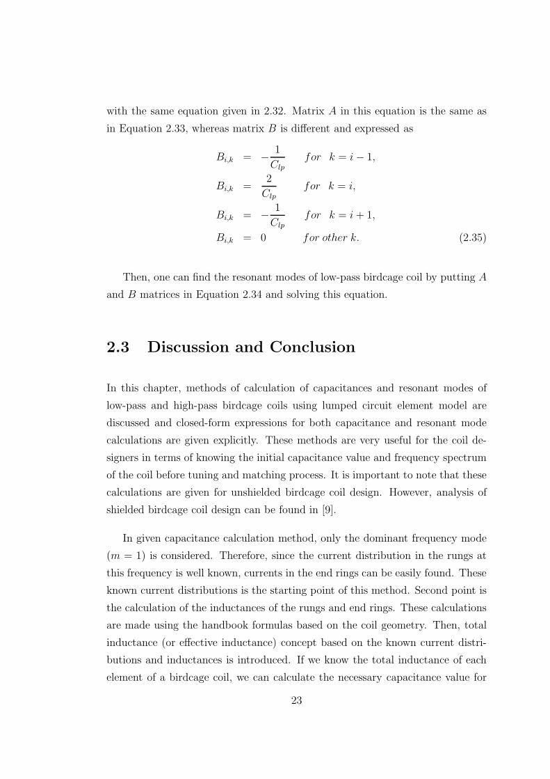
modeled in the simulation environment as shown in Figure 3.1.

Figure 3.1: Low-pass (left) and high-pass (right) birdcage coil geometric models

As given in Figure 3.1, rungs and end-rings are modeled as rectangular strips

without thickness and lumped capacitors are modeled as parallel plate capacitors.

Capacitance value is set by altering the relative permittivity (ǫr) of the material

assigned to the capacitors using the formula

C = ǫ0ǫrA

d(3.1)

where ǫ0 is the permittivity of free space, A is the area of parallel plates and d is

the distance between the parallel plates.

After modeling the geometry of the coils, Electromagnetic Waves interface is

added under the Radio Frequency branch for the physics selection of the model.

26

This interface solves the electromagnetic wave equation for time harmonic and

eigenfrequency problems and the equation is given as

∇× µ−1r (∇× E)− k2

0

(

ǫr −jσ

ωǫ0

)

E = 0 (3.2)

where E is the electric field vector, µr is the relative permeability, σ is the con-

ductivity and k0 is the wave number of free space and is expressed as

k0 = ω√ǫ0µ0 (3.3)

After adding physics for the model, we now need to assign boundary conditions

to the surfaces of coil elements as well as the outer boundary of the solution

domain enclosing the coil geometry. Since the thickness of the copper strip used

to construct birdcage coils is larger than the skin-depth at the frequencies we

are interested in, Perfect Electric Conductors (PEC) is assigned to the rungs and

end-rings boundaries. By assigning this boundary condition, we set the tangential

component of electric field of these boundaries to zero (n× E = 0). In addition

to rungs and end-rings, capacitor plates and RF shield (if exists) boundaries are

also assigned as PEC. PEC boundaries of a low-pass birdcage coil are illustrated

in Figure 3.2.

Figure 3.2: PEC boundaries: Rungs, end rings and capacitor plates (left), RFshield (right)

27

In order to prevent reflections from the outer boundary of the solution domain

(sphere) enclosing the coil geometry, scattering boundary condition or perfectly

matched layer (PML) is used [15] [16]. Among them, scattering boundary con-

dition is applied to the exterior boundaries and make the specified boundary

transparent to outgoing waves. This can be a plane, cylindrical or spherical wave

but for our condition it is a spherical wave. PML, on the other hand, is a type of

domain feature and is used for simulating an infinite domain in which the wave

can propagate and disappear by attenuation without any reflection. In Figure

3.3, boundaries (or layers) of the sphere enclosing the coil geometry are shown.

Figure 3.3: Sphere boundaries assigned to a scattering boundary condition (left),sphere layers are defined as PML (right)

At last, in frequency domain analysis, lumped port boundary condition is

used for voltage excitation [15]. Equation for lumped port boundary condition is

simply given as

Zport =Vport

Iport(3.4)

where Vport is the excited voltage, Iport is the port current, and Zport is the port

impedance. It is important to note that while applying lumped port boundary

condition, lumped port boundary where the voltage or current is applied must be

placed between metallic type boundaries such as PEC. Lumped port boundaries

of one-port and two-port excitations models are shown in Figure 3.4.

28

In eigenfrequency analysis, however, no source is applied to the coil.

Figure 3.4: One-port excitation model (left), two-port excitation model (right).Lumped port boundaries are shown with purple color, PEC boundaries are shownwith red color.

As can be seen in Figure 3.4, voltage is applied from the boundary (shown

with purple colour) which is placed between PEC boundaries (shown with red

colour) and these PEC boundaries are connected to the corresponding capacitor

plates.

After adding physics and boundary conditions, we generate a mesh for the

model in order to discretize the complex geometry of the birdcage coil into tri-

angular and tetrahedral elements. It is important that in electromagnetic wave

problems, wavelength must be taken into consideration while generating a mesh

in order to get accurate results. According to [15], maximum element size of

the mesh elements must be at least one fifth of the wavelength at the interested

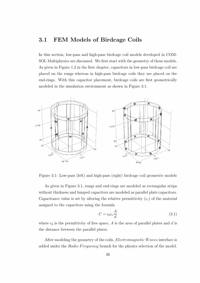
frequency range. Generated mesh of an 8-leg low-pass birdcage model is given as

an example in Figure 3.5.

For the final step, we need to add study and solver sequence for the model

in order compute the solutions. Since this step is about COMSOL Multiphysics

usage, we have decided to explain this step in the following note.

29

Figure 3.5: Generated mesh at the boundary surfaces of the low-pass birdcagemodel (left), x-y plane at z=0 (right)

3.1.0.1 Note: Adding study and solver sequence in COMSOL Multi-

physics

In COMSOL Multiphysics, there are several study types corresponding to the

physics that the user has added. For instance, we have added Electromagnetic

Waves physics interface under the RF module. For this physics interface, we can

choose different studies such as Frequency Domain Study for solving the wave

equation or a frequency response of a model, Time Dependent Study for mak-

ing transient simulations, Eigenfrequency Study for finding resonant modes of a

model or Stationary Study for steady-state analysis of a model. After adding

one of the study types, we need to add necessary solver sequence that corre-

sponds to that study such as Stationary Solver, Time-Dependent Solver, Eigen-

value solver or Optimization Solver. One can also use the default solver sequence

for the corresponding study. For instance, after adding Frequency Domain Study

and specifying necessary parameters such as frequency range, mesh selection and

physics selection, user can solve the model by clicking the Compute button. In

this case, Stationary Solver is automatically added as a solver sequence since it

is the default solver of the Frequency Domain Study. On the other hand, if we

want to make an optimization in our model in Frequency Domain Study, in this

30

case, we need to choose the solver as Optimization Solver instead of using default

solver. Additionally, user can modify the default value of solver parameters such

as relative tolerance which is used for termination of the iterative processes or

linearization point which is used in eigenvalue solver and specifies a point around

where the solution is linearized. After adding study types and solver sequences,

and specifying the necessary parameters from the study and solver settings, we

can compute the solution of a birdcage model that we have developed.

3.2 Methods

In this section, three different electromagnetic analyses of developed birdcage

coils will be discussed.

3.2.1 Frequency Domain Analysis of a Birdcage Coil

We have first made a frequency domain analysis of the developed birdcage models

in COMSOL Multiphysics. As previously mentioned, frequency domain analy-

sis is used to solve for the electromagnetic fields of the birdcage coil at a given

frequency (or frequencies) and can be used for several purposes. For instance,

it can be used to observe any electromagnetic field variables in the model such

as B1 field distribution inside the coil, surface current density in the rungs or

induced currents in the conductive objects. Additionally, one can estimate the

SAR values of any object inside the birdcage coil. Last but not least, instead of

making the simulations at one frequency, one can specify more than one frequen-

cies where the solution will be computed at, in order to observe the variation of

any electromagnetic field parameters with respect to the frequency.

31

3.2.1.1 Linear and Quadrature Excitation

In frequency domain analysis, we have driven the birdcage coil using two differ-

ent excitations: linear and quadrature excitation. As mentioned earlier, in linear

excitation, birdcage coil is driven from one port (shown in Figure 3.4) that gen-

erates a linearly polarized B1 field inside the coil. This linearly polarized field

is the combination of two circularly polarized fields that are left-hand rotating

and right-hand rotating fields. Since the effect of right hand rotating field on

the spins is negligible, we consider only the left hand rotating field, which is also

called excitatory component or positive rotating component of the magnetic field.

In quadrature excitation, on the other hand, birdcage coil is driven from two ports

(shown in Figure 3.4) that are geometrically 90 apart from each other and driv-

ing signals are 90 out of phase that generates a circularly polarized field inside

the coil. The advantage of quadrature excitation of birdcage coils has already

been mentioned in the first chapter.

If we assume that the main magnetic field is in the negative z-direction, the

transmit sensitivity of the coil corresponds to the positively rotating component

of the magnetic field (H+) and the receive sensitivity of the coil corresponds to

the negatively rotating component of the magnetic field (H−) and they can be

expressed as [17]

H+ =Hx + iHy

2

H− =(Hx − iHy)

∗

2(3.5)

where Hx and Hy are the x and y component of the magnetic field respectively

and asterisk indicates the complex conjugate.

3.2.1.2 Study and Solver Sequence

After modeling the low-pass and high-pass birdcage coil as given in Section 3.1,

we need to add study and solver sequence for the model in order to compute the

solutions. For the frequency domain analysis, we first add Frequency Domain

32

Study as study type and specify the frequency range from the study settings.

Then, we choose the Stationary node as the solver sequence and select the bicon-

jugate gradient stabilized (BiCGStab) method with a left pre-conditioner as the

solver [18]. This method is one of the iterative solvers in COMSOL Multiphysics

and is used to solve linear systems of the form Ax = b which is obtained using

Equation 3.2 for the Electromagnetic Waves interface.

3.2.1.3 Simulation Results

First simulation has been made for unshielded and empty 8-leg low-pass birdcage

coil with a diameter of 10 cm, rung length of 11.5 cm, and rung and end-ring width

of 1.5 cm. Capacitance value used on the rungs is 10.3 pF and the simulation

frequency is 123.25 MHz. Total number of degrees of freedom in the equation

system is about 600000. Computations have been performed on a workstation

with 2 Intel Xeon X5675 (3.07GHz) processors and 64GB of memory. Frequency

domain analysis of the model takes about 1 minutes for one frequency.

Geometric model of this coil was given in Figure 3.1. We have made both

linear and quadrature excitation. Magnitude images of H+ and H− at the central

slice (z=0) for linear excitation are given in Figure 3.6.

As can be seen in Figure 3.6, left-rotating and right-rotating components of

the magnetic fields at the specified frequency are the same in linear excitation

case and their combination produces a linearly polarized field inside the coil.

On the other hand, when a birdcage coil is driven from two ports (quadrature

excitation), H− should be zero and H+ >> H−. Magnitude images of H+ and

H− at the central slice (z=0) for quadrature excitation are given in Figure 3.7.

As illustrated in Figure 3.7, H+ is uniform especially at the central region of

the coil and H− is almost zero in the same region in the quadrature excitation.

This is the ideal case for quadrature birdcage coils. In practice, H− never equals

to zero due to the imperfections in birdcage coil geometry, but H+ is still very

much larger than the H−.

33

Figure 3.6: Magnitude images of H+ (left), and H− (right) at the central slice(z=0) for linear excitation

Figure 3.7: Magnitude images of H+ (left), and H− (right) at the central slice(z=0) for quadrature excitation

34

One can also observe the electric field inside the coil for both excitations.

Magnitude images of electric field at the central slice (z=0) for both linear and

quadrature excitations are illustrated in Figure 3.8.

Figure 3.8: Magnitude image of E-field for linear excitation (left), magnitudeimage of E-field for quadrature excitation (right) at the central slice (z=0)

Apart from the field solutions, we can also observe other electromagnetic

variables in the model such as current distribution in the rungs. We know that

currents in the rungs have sinusoidal distribution at the desired frequency. In Fig-

ure 3.9, z-component of the surface current densities in the rungs are illustrated

with the surface arrow plot.

Second simulation has been made for empty and shielded 8-leg low-pass bird-

cage coil with a shield diameter of 14 cm, shield length of 14.5 cm and the rest

are the same with the dimensions used in the first simulation. Used capacitance

value is 14.2 pF and the simulation frequency is 123.25 MHz. Model geometry

for shielded birdcage coil was illustrated in Figure 3.2. Total number of degrees

of freedom in this equation system is about 700000. Computations have been

performed on the same workstation and frequency domain analysis of the model

takes about 1 minutes for one frequency.

By making frequency domain analysis of the shielded coil, we can observe the

effect of the RF shield to the magnetic field homogeneity. For this purpose, we

35

Figure 3.9: Illustration of the current distribution in the rungs with surface arrowplot

have driven the coil as quadrature excitation and compared the |H+| distributionsfor shielded and unshielded cases. For unshielded case, which we have already

performed in the first simulation, magnitude images of H+ at the central slice

(z=0) and the corresponding line plot of |H+| along (x, y=0, z=0) line are shown

in Figure 3.10.

For the shielded case, magnitude images of H+ at the central slice (z=0) and

the corresponding line plot of |H+| along (x, y=0, z=0) line are given in Figure

3.11.

As can be seen in Figure 3.11, uniformity of the H+ increases when the RF

shield, whose length is the same with the coil length and diameter is 1.4 times

of the coil, is used. However, magnitude of the H+ decreases with %13 because

of the eddy currents induced in the shield and produce a magnetic field which is

opposite to H+.

Third simulation has been made for shielded and loaded 16-leg high-pass

birdcage coil with a coil diameter of 24 cm, shield diameter of 28 cm, shield

36

Figure 3.10: Magnitude image of H+ at z=0 slice (left) and |H+| distributionalong the (x, y=0, z=0) line (right) for unshielded low-pass birdcage coil

Figure 3.11: Magnitude image of H+ at z=0 slice (left) and |H+| distributionalong the (x, y=0, z=0) line (right) for shielded low-pass birdcage coil

37

length of 27 cm, rung length of 24 cm, and rung and end-ring width of 1.5 cm.

Capacitance value is 49.4 pF and the simulation frequency is 123.2MHz. We have

put two cylindrical objects with different conductivity values and rectangular

background inside the coil. Background conductivity is also different. Geometry

of the model and the simulation phantom are shown in Figure 3.12.

Figure 3.12: Geometric model of the shielded and loaded 16-leg high-pass birdcagecoil (left) and simulation phantom with the conductivity values (right)

Total number of degrees of freedom in this equation system is about 2 mil-

lion. Computations have been performed on the same workstation and frequency

domain analysis of the model takes about 4 minutes for one frequency.

First, we can observe the magnitude images of the H+ and H− for the loaded

birdcage coil and we can compare these results with the results of unloaded case in

order to see the effects of the conductive objects to the magnetic field. Magnitude

images of H+ at z=0 slice for loaded and unloaded birdcage coils are given in

Figure 3.13.

Figure 3.13 shows that conductive objects inside the coil slightly deteriorates

the uniformity of the H+. We are supposed to see this effect in also H− images.

For this purpose, magnitude images of H− at z=0 slice for loaded and unloaded

birdcage coils are illustrated in Figure 3.14.

38

Figure 3.13: Magnitude images of H+ for unloaded birdcage coil (left) and forloaded birdcage coil (right) at z=0

Figure 3.14: Magnitude images of H− for unloaded birdcage coil (left) and forloaded birdcage coil (right) at z=0

39

By making frequency domain analysis of a loaded birdcage coil, we can also

calculate the SAR distribution of the objects using the formula given as

SAR =σ|E|2ρ

(3.6)

where σ and ρ are the conductivity and density of the object respectively. Nor-

malized SAR distribution image at y=0 slice is shown in Figure 3.15.

Figure 3.15: Normalized SAR distribution image (right) at the slice given on theleft with a red color

In conclusion, one can make accurate simulations and observe the electro-

magnetic fields inside the coil by making frequency domain analysis of developed

loaded (or unloaded) and shielded (or unshielded) birdcage coil models.

3.2.2 Capacitance Calculation of a Birdcage Coil using

FEM based Optimization

In this section, a new method to calculate the necessary capacitance value for the

birdcage coil in order to resonate the coil at the desired frequency is presented.

This method is performed using an optimization with two different objective

function in the frequency domain analysis of a one-port birdcage coil. One of them

finds the capacitance value that maximizes the magnitude of the port impedance

40

(|Z11|) within the given capacitance range. We know that the magnitude of the

port impedance reaches its maximum values at the resonant modes. By giving

reasonable initial value, lower and upper bounds for the capacitance, optimum

capacitance value which maximizes the |Z11| at the desired resonance frequency

can be calculated. The other optimization process is to calculate the capacitance

value that minimizes the variance of H+ at the central region of the coil. We

have already shown that magnetic field distribution inside the coil is uniform,

especially in the central region of the coil, at the desired frequency. By using

this information we can calculate the optimum capacitance value within a given

capacitance range that minimizes the variance of H+. These two optimization

methods will be explained in detail in the following subsections.

3.2.2.1 Capacitance Calculation using |Z11| as an Objective Function

As previously mentioned, |Z11| of a birdcage coil takes its maximum values at the

resonant modes. In order to observe this argument in a simulation environment,

we have made frequency domain analyses of a 8-leg low-pass birdcage coil for the

frequencies ranging from 115 MHz to 230 MHz with a step frequency of 1 MHz

and for a given capacitance value. Simulation results for the |Z11| of this birdcagecoil is illustrated in Figure 3.16.

As can be seen in Figure 3.16, for the constant capacitance value, there are

four peaks of |Z11| corresponding to the four resonant modes (or frequencies) of

the low-pass birdcage coil. As mentioned earlier, we are interested in the lowest

frequency mode for the low-pass birdcage coils.

On the other hand, we can make this simulation by making the frequency

constant and the capacitance value variable which is more appropriate for our

situation since we want to find the capacitance for the known frequency. Simu-

lation results of |Z11| for this condition is shown in Figure 3.17.

In Figure 3.17, for the constant frequency, there are four peaks of |Z11| same

as in Figure 3.16. However, these do not correspond to the different resonant

frequencies at this time since the frequency is constant and only the capacitance

41

Figure 3.16: |Z11| of a 8-leg low-pass birdcage coil with respect to frequency (forthe fixed capacitance)

Figure 3.17: |Z11| of a 8-leg low-pass birdcage coil with respect to capacitance(for the constant frequency)

42

is changing. These are the different resonant modes that degenerates at the given

constant frequency. For example, the peak value surrounded with the red box

in Figure 3.17 implies that m = 1 mode at given frequency is obtained using a

capacitance value about 10 pF. The other peak values implies that m = 2, m = 3,

and m = 4 modes at given frequency are obtained using the capacitance values

24.5, 33, 36 pF respectively. From the view of optimization, |Z11| given in Figure

3.17 is the objective function (or cost function), capacitance value is the control

variable and the task is to find the optimum capacitance value which maximizes

the objective function |Z11| in a given capacitance range. For this purpose, we

have used COMSOL Multiphysics optimization module.

COMSOL Multiphysics uses gradient-based optimization methods and these

methods have some requirements such as that the objective function (or any

constraint function) must be continuous and differentiable with respect to the

control variable [15]. Furthermore, if there are more than one local maxima (or

minima) in the objective function, gradient-based optimization method finds the

one which is closest to initial value of the control variable. Therefore, we need

to define a feasible set for the control variable in order to calculate the correct

capacitance value, for example, red box given in Figure 3.17 can be the feasible

set for our condition since we are interested in the lowest frequency mode.

For this purpose, we have first calculated a capacitance value using lumped

circuit element model. This will be the our initial capacitance value. Before

starting the optimization process, we need to define the lower and upper limits

for the capacitance value. In other words, we need to define a feasible set for the

optimization problem. In order to choose the capacitance range correctly, we have

made frequency domain analysis of a birdcage coil at the desired frequency with

twelve different capacitance whose values around the initial capacitance value.

This analysis is made with a very coarse mesh and therefore it takes about 5

minutes. According to the results of this analysis, we have chosen a feasible

set by looking at the graph of the objective function, |Z11|. Then, we add new

frequency domain analysis study with an optimization solver sequence instead

of stationary solver used in previous section. In the optimization solver, there

43

are two algorithms: Sparse Non-linear OPTimizer (SNOPT) [19] and Levenberg-

Marquardt algorithm [20] [21]. Among them, Levenberg-Marquardt algorithm

can only be used when the objective function is in the least-square form, whereas

SNOPT algorithm, which uses gradient-based optimization techniques, can be

applied to any form of the objective function. Since our objective function, |Z11|,is not in the least-square form, we have used SNOPT algorithm as an optimiza-

tion solver method in the FEM model of birdcage coils. From the solver settings,

we can set the optimization parameters such as optimality tolerance which deter-

mines the termination of the optimization process, maximum number of objective

evaluations, objective contributions (if there are more than one object) and the

gradient method. After adding study and the solver sequence we can start the

optimization process using the FEM models of birdcage coil.

Note that, results for the calculated capacitance values using the proposed

method are given under the Experimental Results chapter in order to compare

the results of proposed method with the results of lumped circuit element model

and the experimental results.

3.2.2.2 Capacitance Calculation using the Variance of H+ as an Ob-

jective Function

As mentioned earlier, magnetic field distribution (H+) inside the birdcage coil,

especially at the central region of the coil, is uniform at the first resonant mode.

Uniformity of the H+ distribution deteriorates as the frequency moves away from

the first resonant mode of the coil. In order to observe this argument in a sim-

ulation environment, we have first define a square plane region at the center of

the birdcage FEM models which is shown in Figure 3.18.

Then, we have made frequency domain analysis at the desired frequency with

different capacitance values and calculated the variance of H+ at this square

shaped boundary for each capacitance value using the formula given as

V ar(H+) =1

SΩ

∫

Ω

|H+ − µ|2dΩ (3.7)

44

Figure 3.18: Geometric model of a 8-leg low-pass birdcage coil with a squareshaped boundary at the center of the coil

where Ω is the surface boundary, SΩ is the area of the boundary, and µ is the

mean (or average) of H+ at this boundary.

Simulation results for the variance ofH+ at this square boundary is illustrated

in Figure 3.19.

As can be seen in Figure 3.19, variance of H+ has only one minimum point

for the given capacitance range. From the view of optimization, we can think

that the variance of H+ is our objective function and the capacitance value is

the control variable. The task is to find the optimum capacitance value which

minimizes the variance of H+ at the boundary which is placed at the center of

the coil.

For this purpose, we have made the same steps as we did in the previous

section for the optimization process. The only difference is to use the variance

of H+ as an objective function instead of using |Z11|. Results for the calculated

capacitance values using the proposed method are given under the Experimental

Results chapter.

45

Figure 3.19: Variance of H+ at the square plate with respect to capacitance

3.2.3 Eigenfrequency Analysis of a Birdcage Coil

In this section, eigenfrequency analysis of a birdcage coil, which is used to deter-

mine the resonant modes of the birdcage coil, is presented. Same as the previous

methods, we use developed FEM models of low-pass and high-pass birdcage coil

in this analysis. Model geometry is a bit different than the model geometry con-

structed in the frequency domain analysis. In eigenfrequency analysis, no sources

are applied and therefore we do not use the lumped port boundary condition for

this analysis. Geometric model of the low-pass and high-pass birdcage coil used

in eigenfrequency analysis are shown in Figure 3.20.

As can be seen in Figure 3.20, no lumped port boundary is used to apply

voltage. There are only parallel plate capacitors placed on the rungs or end

rings.

Electromagnetic wave equation used in the time harmonic and eigenfrequency

problems was given in Equation 3.2. In the case of eigenfrequency analysis ω is

the unknown variable in Equation 3.2 and the eigenvalue, λ, can be expressed in

46

Figure 3.20: Geometric model of unshielded 8-leg low-pass birdcage coil (left) andshielded 16-leg high-pass birdcage coil (right) used in eigenfrequency analysis

terms of ω as

−λ = −δ + jω (3.8)

where imaginary part of the eigenvalue, ω, corresponds to the eigenfrequency and

the real part, δ, represents the damping factor. Eigenvalue can be complex valued

as given in Equation 3.8 when the model includes some lossy parts such as con-

ductive objects, when boundaries are modeled as scattering boundary condition,

or when domains are modeled as perfectly matched layers. In a such condition,

we can express the quality factor (Q) in terms of eigenfrequency and damping

factor as

Q =ω

2|δ| (3.9)

It is important to note that we can calculate the Q-factor of the birdcage coil

using the Equation 3.9.

After modeling the coil geometry, adding physics and boundary conditions,

and generating mesh as explained in the first section of this chapter, we need

to add necessary study and the solver sequence for eigenfrequency analysis in

COMSOL Multiphysics. This step is explained under the following subsection.

47

3.2.3.1 Study and Solver Sequence

For eigenfrequency analysis, we first add Eigenfrequency Study as the study node.

From the study settings, we can define the number of eigenfrequencies which

the solver finds and the frequency point around which the solver looks for the

eigenfrequencies. Then, we add Eigenvalue Solver as the solver sequence to solve

the FEM based generalized eigenvalue system which is given as [15]

(λ− λ0)2EU − (λ− λ0)DU +KU +NFΛ = 0 (3.10)

NU = 0 (3.11)

where λ is the eigenvalue, λ0 is the linearization point, E is the mass matrix, U

is the solution vector, D is the damping matrix, K is the stiffness matrix, NF is

the constraint force Jacobian matrix, Λ is the Lagrange multiplier vector, and N

is the constraint Jacobian matrix. If the mass matrix (E) in Equation 3.10 is 0,

eigenvalue problem will be linear. If E is non-zero, eigenvalue problem will be

quadratic which needs a special treatment to transform the problem into a linear

eigenvalue problem.

Eigenvalue solver starts the computation of the eigenfrequencies by linearizing

the problem around the linearization point, whose default value is 0. In non-

linear eigenfrequency problems, using this default value of the linearization point

causes an error because the λ is generally in the denominator in the equation

system and leads to division by zero. In our situation, using scattering boundary

condition leads to this problem and therefore we need to specify a linearization

point (λ0) in order to avoid this problem. Instead of specifying the linearization

point manually, we can use the solution of any study as the linearization point of

the eigenfrequency study.

After making the necessary adjustments for the study and solver sequence, we

can compute the eigenfrequencies of the model which correspond to the resonant

modes of the birdcage coil. We can also observe the electromagnetic field or

variable distributions at these resonant modes. Simulation results are given in

the following section.

48

3.2.3.2 Simulation Results

First simulation has been made for unshielded and empty 8-leg low-pass birdcage

coil with a diameter of 10 cm, rung length of 11.5 cm, and rung and end-ring

width of 1.5 cm. Capacitance value used on the rungs is 10.3 pF. Number of

eigenfrequencies is specified as 8 and the linearization point is given as (−j2π120×106). Total number of degrees of freedom in the equation system is about 600000.

Computations have been performed on the same workstation and eigenfrequency

analysis of the model takes about 10 minutes.

There are four distinct resonant modes calculated in this eigenfrequency anal-

ysis. Results for the magnitude images ofH+ inside the coil at these four resonant

modes are given in Figure 3.21.

As can be seen in Figure 3.21, calculated eigenfrequencies are complex valued

in which the real part corresponds to under-damped natural resonance frequency,

f0, and the imaginary part represents the damping factor, δ. We can find the

damped natural resonance frequency, fd, using the equation given as

fd = f0√

1− ζ2 (3.12)

where ζ is the damping ratio and defined as

ζ =δ

2πf0(3.13)

Since δ << f0 for the calculated eigenfrequencies given in Figure 3.21, we can

write the damped natural frequency as fd ≈ f0. Therefore we can say that first

resonant mode of the coil, which is the desired mode (m = 1), is found at 123.27

MHz, and the other modes, m = 2, 3, and 4, are found at 182.57 MHz, 211.83

MHz, and 220.84 MHz respectively.

As mentioned earlier, we have found four distinct resonant modes for 8-leg

low-pass birdcage coil. Among these modes, m = 1, 2, and 3 are the degenerate

mode pairs and m = 4 is the singlet mode. We know that, degenerate mode pairs

are actually two modes that have the same resonance frequency but represented

49

Figure 3.21: Magnitude images of H+ at the resonant modes of the coil. (m=1(left-top), m=2 (right-top), m=3 (left-bottom), and m=4 (right-bottom))

50

with the single m and these two modes produces magnetic fields which are per-

pendicular to each other. We can also observe these two magnetic fields in this

analysis. For m = 1 mode, magnitude images of H+ at these two resonant modes

are given with the surface arrow plots in Figure 3.22.

Figure 3.22: Magnitude images of H+ for the frequencies found at 123.276 MHz(left) and 123.299 MHz (right) of m = 1 mode

Second simulation has been made for shielded and empty 16-leg high-pass

birdcage coil with a coil diameter of 24 cm, shield diameter of 28 cm, shield

length of 27 cm, rung length of 24 cm, and rung and end-ring width of 1.5 cm.

Capacitance value is 49.4 pF. Number of eigenfrequencies is specified as 16 and

the linearization point is given as (−j2π120 × 106). Total number of degrees

of freedom in this equation system is about 2 million. Computation has been

performed on the same workstation and have taken about 35 minutes.

There are eight distinct resonant modes calculated in this eigenfrequency

analysis. Instead of observing these modes as we did in the previous simula-

tion, we want to investigate another mode, which is previously mentioned as

co-rotating/anti-rotating or end ring resonant mode, m = 0. In this mode, cur-

rents flow only in the end rings so that no transverse electromagnetic field is

produced inside the coil. Eigenfrequency analysis can also calculate this mode

and we can observe the field distribution at the transverse plane and current

51

distribution in the rungs and end rings. Magnitude images of H+ at the central

slice (z=0) and the arrow plot of surface current density in rungs and end rings

at two frequencies of m = 0 mode are illustrated in Figure 3.23.

Figure 3.23: Magnitude images of H+ and the arrow plot of surface currentdensities for the frequencies found at 150.518 MHz (left) and 150.581 MHz (right)of m = 0 mode

As can be seen in Figure 3.23, m = 0 has two modes as the other degenerate

mode pairs. One of these modes corresponds to the co-rotating mode in which

the currents in the end rings are rotating in the same direction and the other

mode corresponds to the anti-rotating mode in which the currents in the end

rings are in the opposite direction. Since no current flows in the rungs, transverse

magnetic field inside the coil shown in Figure 3.23 is significantly small.

In conclusion, one can calculate the resonant modes of the birdcage coil and

observe any electromagnetic fields and variables at these resonant modes. Simula-

tion results of the eigenfrequency analysis will be compared with the experimental

results and the results of the lumped circuit element model under the Experimen-

tal Results chapter.

52

3.3 Discussion and Conclusion

In this chapter, we have presented the development of low-pass and high-pass

birdcage coil FEM models and three simulation methods which are performed

using these models in COMSOL Multiphysics.

First method is the frequency domain analysis which is used to simulate prac-

tical birdcage coils used in MRI for a given frequency and the capacitance value.

By performing this analysis, one can calculate the electromagnetic fields inside

the birdcage coil for any scenario and produce simulated B1 data which is widely

used in the MR based electromagnetic tissue property mapping algorithms such

as MREPT. Furthermore, this analysis can be used to simulate loaded birdcage

coils at higher frequencies in order to investigate the SAR at any object at these

frequencies. Additionally, one can investigate how geometric changes in the coil

elements or the objects that have different material properties inside the coil

affects the field solutions of the birdcage coil. Since the field strength of MRI

Scanner in Ulusal Manyetik Rezonans Aratrma Merkezi (UMRAM) that we use

for our MR experiments is about 2.893 T , simulation results are given at 123.2

MHz for practice. The important point here is to find the necessary capacitance

value which makes the coil resonate at 123.2MHz. This is accomplished by using

the second method we have proposed.

Second method is the capacitance calculation of a birdcage coil using FEM

based optimization. In this method, optimum capacitance value at given reso-

nance frequency is calculated using an optimization with two different objective

functions: |Z11| and the variance of H+. By looking at these two objective func-

tions given in Figure 3.17 and Figure 3.19 respectively, we can see that |Z11| inFigure 3.17 forms sharp peaks, whereas the variance of H+ in Figure 3.19 forms

a shallow minimum. Since we want to find the capacitance value which maxi-

mizes (or minimizes) the objective function, using |Z11| as an objective function

will give more reliable results because the numerical errors in the computation

is more dominant at the shallow regions and this may lead to misdetection of

the minimum value of the variance of H+. On the other hand, using only |Z11|as an objective function may also give wrong results if the objective function

53

includes more than one maximum point in the given set. Therefore, we can use

the variance of H+ to determine the feasible set since it has only one minimum

point. Then, we can make the optimization using |Z11| as an objective function

with this determined set. We believe that this approach will help to eliminate

any possible errors in the optimization process.

Third method is the eigenfrequency analysis which is used to calculate not

only the resonant modes of the birdcage coil but also the electromagnetic fields or

variables distributions at these resonant modes. This analysis provides informa-

tion about the resonance behavior of the coil and therefore tuning and matching

procedure of the working mode (m = 1) can be safely done without interfering

with the other modes. Further more, we can also determine the quality factor

of the birdcage coil loaded with a conductive object by making eigenfrequency

analysis.

Before comparing the results of these three methods with the experimental

results and lumped element model results, we need to be sure that they are first

consistent with each other. For this purpose, we have made some trials. For ex-

ample, we have used the capacitance value, which is calculated using FEM based

optimization at given frequency, in the eigenfrequency analysis and compared the

first resonant frequency calculated in eigenfrequency analysis with the frequency

given in FEM based optimization. We have also made a frequency domain anal-

ysis for the capacitance, which is calculated by using FEM based optimization

method, and checked if the H+ is uniform or not for this capacitance value in

the frequency domain analysis. In the end, we are sure that they are perfectly

consistent with each other.

In order to provide convenience for the coil designers and the researchers in the

field of MRI to make these three simulation methods easily and according to the

parameters they specify, we have developed two user-friendly software tools using

MATLAB GUI which connect to the COMSOL Multiphysics server and make all

the FEM based design and simulations in the background. These software tools

will be explained in the next chapter.

54

Chapter 4

SOFTWARE TOOLS FOR

DESIGNING AND

SIMULATING A BIRDCAGE

COIL

In this chapter, two different software tools, that we have developed to make the

FEM based simulation methods explained in the previous chapter according to

the user-specified parameters easily, are presented. One of the software tools is

used to calculate the capacitance value of a birdcage coil using the FEM based

optimization method and the other one is used to make frequency domain and

eigenfrequency analysis of a birdcage coil. Both of the software tools have been

developed in MATLAB and have user-friendly graphical user interface (GUI).

User can make any of the three simulation methods for any type of birdcage coil

by only specifying the coil type, dimensions and necessary parameters from the

GUI of the program. Then, software tools make all the design and simulation

steps such as modeling the coil geometry, adding physics and boundary condi-

tions, generating mesh and computing the solutions by connecting the COMSOL

Multiphysics server in the background. When the simulation is finished, the user

can import the model from the server and observe the any electromagnetic fields

55

and variables in the solution domain. In the following two sections, these software

tools will be explained in detail.

4.1 A Software Tool for Frequency Domain and

Eigenfrequency Analysis of a Birdcage Coil

First software tool is used to make two electromagnetic analyses of a birdcage

coil: frequency domain and eigenfrequency analyses. GUI of the program is given

in Figure 4.1.

Figure 4.1: Graphical User Interface (GUI) of the software tool used in frequencydomain and eigenfrequency analyses

As can be seen in Figure 4.1, there are three sections of this software tool:

Design parameters, simulation parameters and results.

The user first starts with specifying the design parameters that are coil type,

56

number of legs and coil dimensions. For the unshielded birdcage coil simula-

tions, RF shield radius must be specified as zero. Then, by clicking the Design

button, the tool calculates the necessary capacitance value using lumped circuit

element model and calculated capacitance value appears in the results section of

the program.

Second, simulation parameters should be specified. For this purpose, the user

starts with selecting the study type and specifying the parameters that corre-

spond to selected study. If frequency domain analysis is chosen, for example,

frequency range for this analysis must be specified. In order to make a frequency

domain analysis at a single frequency, start and stop frequency should be the

same and equal to the frequency at which the simulation is made and the fre-

quency step can be any value other than zero. Then, the user chooses one of the

boundary conditions for the solution domain to prevent reflections from the outer

boundary and selects the excitation type in order to produce linearly or circularly

polarized field inside the birdcage coil. If eigenfrequency analysis is chosen, on

the other hand, the user should specify the number of eigenfrequencies, which

the solver finds, and the frequency point around which the solver looks for the

eigenfrequencies. Since no source is applied in eigenfrequency analysis, excitation

part is disabled. For both analysis, desired mesh size is selected from the mesh

selection part. Before the simulation starts, the user can specify different value

for the capacitance whose default value is calculated using lumped circuit element

model. After all the necessary parameters are specified, the user can start the

simulation by clicking the Simulate button.

When the simulation is started, the program connects to the COMSOL Mul-

tiphysics server via COMSOL Multiphysics Livelink for MATLAB environment

and makes the FEM based design and simulations according to the user-specified

parameters. During the simulation, the tool informs the user about which step

is being performed at that moment by displaying the step in the results section.

When the simulation is finished, the program notifies the user and simulation

results can be observed in COMSOL Multiphysics by importing the computed

model from the server. It is important to note that simulation results can also be

57

observed in MATLAB environment but displaying the results in COMSOL Multi-

physics is easier and also offers to make changes in the model. For example, after

making frequency domain analysis of 16-leg high-pass birdcage coil by using this

software tool, we can import the computed model to the COMSOL Multiphysics

environment, put any arbitrary object inside coil and make the simulation for

loaded birdcage coil easily.

4.2 A Software Tool for Capacitance Calcula-

tion of a Birdcage Coil

The other software tool is used to calculate the necessary capacitance value of a

birdcage coil in order to resonate the coil at the specified frequency. GUI of the

program is illustrated in Figure 4.2

Figure 4.2: Graphical User Interface (GUI) of the software tool used in capaci-tance calculation

As given in Figure 4.2, this software tool has three sections. One of the

sections, in which the user specify the coil parameters, are the same with the

previous one. After specifying the coil parameters, the user chooses the mesh size

and define the optimality tolerance from the optimization parameters section.

58

As previously mentioned, optimality tolerance determines when the optimization

process terminates. After specifying all necessary parameters, optimum capaci-

tance value can be calculated by clicking the Calculate button.

When the simulation starts, the program first calculates a capacitance value

using lumped circuit element model. This capacitance value is used to define a

capacitance range for the next step which is the frequency domain analysis of a

birdcage coil with a very coarse mesh for twelve different capacitance values. This

is called parametric sweep study in which the capacitance value is the variable

parameter. At the end of this study, the program displays two objective functions,

|Z11| and V ar(H+), with respect to capacitance and asks the user which objective

function will be used for the optimization process. As an example, parametric

study results for the birdcage coil, whose properties and dimensions are given as

in Figure 4.2, is illustrated in Figure 4.3.

Figure 4.3: Parametric study results of the objective functions: |Z11| (left), vari-ance of H+ (right)

When the user chooses one of the objective functions, the program wants from

the user to specify the initial value, lower and upper bounds for the capacitance

to be used in the optimization process. This selection is performed by clicking

the three points, which are corresponding to lower bound, initial value and upper

bound respectively, on the selected objective function figure. This selection is

illustrated in Figure 4.4 for the objective function, |Z11|.

59

Figure 4.4: Illustration of the selection of the lower bound (left), initial value(middle), and upper bound (right) for the capacitance value

After specifying the capacitance ranges, program starts to optimization pro-

cess with the specified mesh size. When the simulation is finished, initial value

given for the capacitance and the calculated capacitance are shown in the results

section, which can be seen in Figure 4.2.

4.3 Discussion and Conclusion

In this chapter, we have presented two software tools that are used to make design

and simulation calculations of a low-pass and high-pass birdcage coil easily. We

believe that these software tools provide many conveniences to the users. For

example, modeling a birdcage coil in a 3D simulation environment is a difficult

task because of the complex geometry of the birdcage coil. By using these software

tools, any birdcage coil is modeled geometrically, necessary boundary conditions

are assigned to the coil elements, mesh and study properties are set automatically.

As a result, the user can perform any of the simulation methods discussed in

Chapter 3 properly.

The program codes are written in MATLAB and COMSOL Multiphysics

Livelink for MATLAB environment is used. Using this environment provides us to

perform any COMSOL actions in MATLAB. When the simulations are finished,

computed models can be imported from the server to the COMSOL Multiphysics

and any electromagnetic field and variable distribution can be observed.

60

Chapter 5

EXPERIMENTAL RESULTS

AND COMPARISON WITH

NUMERICAL ANALYSES

In this chapter, experimental results for the resonant modes and capacitance

values of two handmade birdcage coils are presented. These coils are low-pass and

high-pass birdcage coils and they are illustrated in Figure 5.1 without capacitors.

As can be seen in Figure 5.1, they are both 8-leg birdcage coils with a diameter

of 10 cm and are built on plexiglass tubes with a length of 16.5 cm. The width of

the copper strips used to construct rungs and end-rings is 1.5 cm. Rung length

of the low-pass birdcage coil is about 11.55 cm, whereas rung length of the high-

pass birdcage coil is about 11.25 cm. They are both constructed as one-port and

unshielded birdcage coil.

Experimental results can be discussed under two sections. One of them is the

results of the resonant modes of the birdcage coils. For this purpose, we have

made measurements for five different capacitance values (Dielectric Laboratories

High-Q Multi-Layer and Broadband Blocking Capacitors) for each birdcage coil

and measured the S11 of the coils using Agilent Technologies E5061A (300 kHz

- 1.5 GHz) Network Analyzer in order to obtain the resonant modes of the coil.

61

Figure 5.1: Constructed two handmade birdcage coils. Low-pass type (left) andhigh-pass type (right)

Then, these experimental results are compared with the results of the software

tool called MRIEM presented in [9] and the results of FEM based eigenfrequency

analysis tool (FEM-EFAT) we have proposed. The other section is the comparison

of the capacitance values used in the experiments with the capacitance values

calculated using the software tool called BirdcageBuilder presented in [5] and

FEM based optimization tool (FEM-OPT) we have proposed.

5.1 Measured and Calculated Resonant Modes

In this section, experimental results for the resonant modes of the unshielded

8-leg low-pass and high-pass birdcage coils, which are shown in Figure 5.1, are

presented for five different capacitance values. Then, these experimental results

are compared with the results of MRIEM (a software tool that uses the lumped

circuit element model presented in [9], and can be downloaded from the link

62

http://jin.ece.illinois.edu/mriem.dir/mriem.html) and the results of FEM-EFAT

we have developed.

5.1.1 Results of the High-pass Birdcage Coil

In order to compare the measured and calculated results of the resonant modes

of 8-leg high-pass birdcage coil, the results for each capacitance value are given in

a separate table. For the capacitance value of 100 pF (±%2), 30 pF (±%2), 15

pF (±%2), 7.5 pF (±0.25pF ), and 3.3 pF (±0.25pF ), measured and calculated

resonant modes are given in Tables 5.1 to 5.5 respectively.

Modes Experimental Results (MHz) MRIEM (MHz) FEM-EFAT (MHz)m=4 52.13 51.91 52.67m=3 53.63 54.24 54.58m=2 59.63 62.82 61.11m=1 75.25 86.14 75.36m=0 107.6 - 108.3

Table 5.1: Measured and calculated resonant modes of 8-leg high-pass birdcagecoil for the capacitance of 100 pF

Modes Experimental Results (MHz) MRIEM (MHz) FEM-EFAT (MHz)m=4 94.43 94.76 95.58m=3 97.33 99.03 99.02m=2 106.0 114.68 110.74m=1 131.4 157.27 136.18m=0 195.2 - 196.06

Table 5.2: Measured and calculated resonant modes of 8-leg high-pass birdcagecoil for the capacitance of 30 pF

Modes Experimental Results (MHz) MRIEM (MHz) FEM-EFAT (MHz)m=4 131.2 134.02 134.1m=3 134.0 140.05 138.87m=2 143.8 162.19 155.08m=1 182.5 222.41 189.92m=0 264.2 - 275.1

Table 5.3: Measured and calculated resonant modes of 8-leg high-pass birdcagecoil for the capacitance of 15 pF

63

Modes Experimental Results (MHz) MRIEM (MHz) FEM-EFAT (MHz)m=4 182.1 189.53 186.56m=3 187.2 198.07 193.04m=2 200.8 229.37 215.00m=1 245.0 314.53 261.16m=0 370.1 - 382.64

Table 5.4: Measured and calculated resonant modes of 8-leg high-pass birdcagecoil for the capacitance of 7.5 pF

Modes Experimental Results (MHz) MRIEM (MHz) FEM-EFAT (MHz)m=4 256.0 299.68 270.36m=3 266.0 313.17 279.23m=2 294.0 362.66 308.76m=1 334.26 497.32 368.01m=0 516.0 - 553.02

Table 5.5: Measured and calculated resonant modes of 8-leg high-pass birdcagecoil for the capacitance of 3.3 pF

Using these results, we can calculate the percentage error of the results of

the two software tools relative to the values obtained experimentally using the

formula

Error rate (%) = 100×∣

∣

∣

∣

fmeas − fcalcfmeas

∣

∣

∣

∣

(5.1)

where fmeas is the measured frequency in the experiment and fcalc is the calculated

frequency using one of the software tools, MRIEM or FEM-EFAT. Percentage

errors of the results of these software tools are shown in Figure 5.2.

As can be seen in Figure 5.2, resonant modes calculated using the FEM-

EFAT are more accurate compared with the experimental results. For the worst

case scenario, in which the used capacitance value is 3.3 pF with a tolerance of

±0.25pF and the wavelength is comparable with the coil dimensions, our software

tool calculates the resonance frequencies with a maximum of % 10 error, whereas

MRIEM calculates the first resonant modes with % 50 error. As previously men-

tioned, when the wavelength is comparable with the coil dimensions, calculation

of the resonant modes using lumped circuit element model will give unreliable

results. We can see this phenomena in the MRIEM results given in Figure 5.2 as

the capacitance used in the experiment decreases (or the resonance frequencies

64

Figure 5.2: Percentage error rate of the two software tools: FEM-EFAT (left),MRIEM (right)

are increases), error in the calculated resonant modes significantly increases. Ad-

ditionally, FEM-EFAT calculates the end ring resonant mode (m = 0), whereas

MRIEM does not calculate the m = 0 mode.

5.1.2 Results of the Low-pass Birdcage Coil

Same as the high-pass birdcage coil results, the results of the resonant modes

of the low-pass birdcage coil are given in a separate tables for five different ca-

pacitance values which are 47 pF (±%2), 10 pF (±%2), 3.3 pF (±0.25pF ), 1.8

pF (±0.25pF ), and 1 pF (±0.25pF ). Resonant modes results of the low-pass

birdcage coil for these capacitance values are given in Table 5.6 to 5.10.

Modes Experimental Results (MHz) MRIEM (MHz) FEM-EFAT (MHz)m=1 60.75 67.46 59.1m=2 85.88 90.64 87.22m=3 93.38 102.2 101.1m=4 102.8 - 105.4

Table 5.6: Measured and calculated resonant modes of 8-leg low-pass birdcagecoil for the capacitance of 47 pF

65

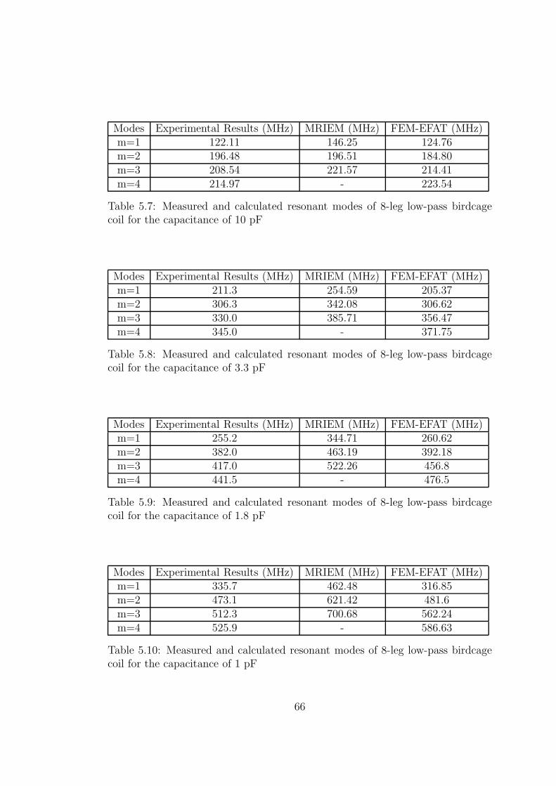
Modes Experimental Results (MHz) MRIEM (MHz) FEM-EFAT (MHz)m=1 122.11 146.25 124.76m=2 196.48 196.51 184.80m=3 208.54 221.57 214.41m=4 214.97 - 223.54

Table 5.7: Measured and calculated resonant modes of 8-leg low-pass birdcagecoil for the capacitance of 10 pF

Modes Experimental Results (MHz) MRIEM (MHz) FEM-EFAT (MHz)m=1 211.3 254.59 205.37m=2 306.3 342.08 306.62m=3 330.0 385.71 356.47m=4 345.0 - 371.75

Table 5.8: Measured and calculated resonant modes of 8-leg low-pass birdcagecoil for the capacitance of 3.3 pF

Modes Experimental Results (MHz) MRIEM (MHz) FEM-EFAT (MHz)m=1 255.2 344.71 260.62m=2 382.0 463.19 392.18m=3 417.0 522.26 456.8m=4 441.5 - 476.5

Table 5.9: Measured and calculated resonant modes of 8-leg low-pass birdcagecoil for the capacitance of 1.8 pF

Modes Experimental Results (MHz) MRIEM (MHz) FEM-EFAT (MHz)m=1 335.7 462.48 316.85m=2 473.1 621.42 481.6m=3 512.3 700.68 562.24m=4 525.9 - 586.63

Table 5.10: Measured and calculated resonant modes of 8-leg low-pass birdcagecoil for the capacitance of 1 pF

66

According to these results, we can calculate the percentage error of the results

of the software tools for each mode using the formula given in Equation 5.1 and

this is illustrated in Figure 5.3.

Figure 5.3: Percentage error rate of the two software tools: FEM-EFAT (left),BirdcageBuilder (right)

As can be seen in Figure 5.3, results of the FEM-EFAT is also more accurate

than the results of MRIEM software tool in low-pass birdcage coils type. For the

m = 1 mode, FEM-EFAT calculates the resonance frequencies with a maximum

of % 8 error, whereas MRIEM calculates with % 37 error for the worst case.

Additionally, FEM-EFAT calculates the singlet mode (m = 4) of the low-pass

birdcage coil, whereas MRIEM does not calculate the singlet mode (m = 4)

although its calculation is given in [9]. At last, error in the MRIEM results

increases when the capacitance value decreases which is the same phenomena

observed in the MRIEM results for the high-pass birdcage coil.

5.2 Used and Calculated Capacitance Values

In this section, we have estimated the necessary capacitance value for the

same low-pass and high-pass birdcage coils for five different resonance frequen-

cies. These are the measured resonance frequencies for the m = 1 mode cor-

responding to the capacitance values of 100 pF, 30 pF, 15 pF, 7.5 pF, and

67

3.3 pF for the high-pass birdcage coil, and corresponding to the capacitance

values of 47 pF, 10 pF, 3.3 pF, 1.8 pF, and 1 pF for the low-pass bird-

cage coil used in the previous experiment. We have compared these capaci-

tance values used in the experiments with the capacitance values calculated us-

ing two different software tools, which are our FEM based optimization tool

(FEM-OPT) and BirdcageBuilder (a software tool that uses the lumped cir-

cuit element model presented in [5], and can be downloaded from the link,

http://pennstatehershey.org/web/nmrlab/resources/software/birdcagebuilder).

Results for the high-pass birdcage coil are given in Table 5.11.

Frequency Experiment (pF) BirdcageBuilder (pF) FEM-OPT (pF)75.25 MHz 100 99.27 100.34131.4 MHz 30 32.56 32.3182.5 MHz 15 16.88 16.03245.0 MHz 7.5 9.36 8.65334.26 MHz 3.3 5.03 4.2

Table 5.11: Used and calculated capacitance values of high-pass birdcage coil

Percentage error of the results of these two software tools can be calculated

using the formula given as

Error rate (%) = 100×∣

∣

∣

∣

Cexp − Ccalc

Cexp

∣

∣

∣

∣

(5.2)

where Cexp and Ccalc are the used and calculated capacitance respectively and it

is illustrated in Figure 5.4.

Figure 5.4: Percentage error of the software tools for the high-pass birdcage coil

68

As can be seen in Figure 5.4, error in the results of the both software tools

increases when the desired frequency increases. However, increase in the error

of the BirdcageBuilder results is significantly greater than the increase in the

error of FEM-OPT results. Therefore, we can say that the results of the FEM-

OPT is more accurate than the results of the BirdcageBuilder. For the worst

case scenario, for example, FEM-OPT calculates the capacitance value with %

25 error, whereas BirdcageBuilder calculates with more than % 50 error. This is

the expected result for the BirdcageBuilder since this method uses lumped circuit

element model and inductance calculations will not be correct as the frequency

increases.

Calculated capacitance values for the low-pass birdcage coil, on the other

hand, are given in Table 5.12.

Frequency Experiment (pF) BirdcageBuilder (pF) FEM-OPT (pF)60.75 MHz 47 43.87 44.42122.11 MHz 10 10.86 10.46211.3 MHz 3.3 3.63 3.51255.2 MHz 1.8 2.49 1.92335.7 MHz 1 1.44 0.84

Table 5.12: Used and calculated capacitance values of low-pass birdcage coil

Using the formula given in Equation 5.2, percentage error of the results of the

software tools for low-pass birdcage coil can be obtained as given in Figure 5.5.

Figure 5.5: Percentage error of the software tools for the low-pass birdcage coil

Figure 5.5 shows that results of the FEM-OPT is also more accurate than

69

the results of the BirdcageBuilder for the low-pass birdcage coil. It is important

to note that results for the capacitance values of 1 pF and 1.8 pF may not be

taken into account, since the tolerance of these capacitances is ±0.25 pF and this

may affect the results significantly. Even if we do not take the results of these

capacitances into consideration, results of FEM-OPT is still more accurate than

the results of BirdcageBuilder.

70

Chapter 6

CONCLUSIONS

In this thesis, analysis of a birdcage coil using lumped circuit element model and

using the developed 3D FEM models of low-pass and high-pass birdcage coils

are explained. Three different FEM based simulation methods for designing and

simulating the birdcage coils accurately in COMSOL Multiphysics are proposed.

In the design process, a new method for the capacitance calculation of a bird-

cage coil at the specified frequency is presented. In this method, we perform a

FEM based optimization study using the magnitude of the port impedance of the

birdcage coil model or the variance of the H+ in the central region of the bird-

cage coil model as the objective function and the capacitance value as the control

variable. As a consequence of this study, optimum capacitance value which maxi-

mizes (or minimizes) the objective function is calculated. Additionally, a software

tool called FEM based OPtimization Tool (FEM-OPT) is developed in order to

perform this method according to the user-specified parameters easily. Experi-

mental results for the calculated capacitances show that the results of FEM-OPT

are more accurate than the results of the other software tool (BirdcageBuilder)

that uses lumped circuit element model. In low frequencies, where the coil di-

mensions is much smaller than the wavelength, the results of FEM-OPT and the

results of BirdcageBuilder are almost the same. Therefore, users can use any of

these software tools in order to calculate the capacitance value of a birdcage coil

71

for low frequencies. In high frequencies, however, where the wavelength is com-

parable with the coil dimensions, FEM-OPT gives more accurate results than the

BirdcageBuilder. This is because the inductance calculations in lumped circuit

element model are made under quasi-static assumptions and therefore error will

increase as the desired resonance frequency increases. In FEM-OPT, on the other

hand, we have made no assumptions while we are modeling the birdcage coils in

the FEM simulation environment but we need to take into consideration of the

size of the mesh elements. In order to obtain accurate results in FEM-OPT,

maximum element size of the mesh elements must be at least one fifth of the

wavelength.

In the simulation process, we have proposed two different electromagnetic

analyses of birdcage coils. One of them is the frequency domain analysis and is

used to solve for electromagnetic fields of a birdcage coil. By using this analysis,

we can observe the electromagnetic fields inside the birdcage coil for any scenario

such as loaded or shielded birdcage coil. Furthermore, this analysis can be used

to estimate SAR at any object inside the coil or can be used to produce simulated

B1 data. The other electromagnetic analysis is the eigenfrequency analysis and is

used to determine the resonant modes of the birdcage coil. One can also observe

the electromagnetic field or other electromagnetic variable distributions inside

the coil at these resonant modes in the eigenfrequency analysis. Furthermore,

quality factor for the loaded or unloaded birdcage coils can be calculated using this

analysis. Additionally, in order to perform both analysis according to the user-

specified parameters easily, software tool called FEM based Frequency Domain

Analysis (FEM-FDA) and FEM based EigenFrequency Analysis (FEM-EFAT) is

developed. Experimental results for the calculated resonant modes show that the

results of the FEM-EFAT are more accurate than the results of the other software

tool (MRIEM) that uses lumped circuit element model. Since MRIEM uses the

lumped circuit element model same as the BirdcageBuilder, error in the results

of MRIEM significantly increases as the frequency increases.

Consequently, FEM based simulation methods and the corresponding software

tools, which are proposed in this thesis, can be used to design and simulate the

low-pass and high-pass birdcage coils accurately. These methods can be easily

72

adapted to design and simulate other RF coils such as transverse electromagnetic

(TEM) coils and phased-array coils.

73

Bibliography

[1] C. Hayes, W. Edelstein, J. Schenck, O. Mueller, and M. Eash, “An efficient,

highly homogeneous radiofrequency coil for whole-body NMR imaging at 1.5

T,” Journal of Magnetic Resonance, vol. 63, pp. 622–628, 1985.

[2] C. Chen, D. Hoult, and V. Sank, “Quadrature detection coils–a further√2 improvement in sensitivity,” Journal of Magnetic Resonance, vol. 54,

pp. 324–327, 1983.

[3] M. C. Leifer, “Resonant modes of the birdcage coil,” Journal of Magnetic

Resonance, vol. 124, pp. 51–60, 1997.

[4] G. Giovannetti, L. Landini, M. Santarelli, and V. Positano, “A fast and accu-

rate simulator for the design of birdcage coils in MRI,” Magnetic Resonance

Materials in Physics, Biology and Medicine, vol. 15, pp. 36–44, 2002.

[5] C.-L. Chin, C. M. Collins, S. Li, B. J. Dardzinski, and M. B. Smith, “Bird-

cagebuilder: Design of specified-geometry birdcage coils with desired current

pattern and resonant frequency,” Concepts in Magnetic Resonance, vol. 15,

no. 2, pp. 156–163, 2002.

[6] J. Tropp, “The theory of the bird-cage resonator,” Journal of Magnetic Res-

onance, vol. 82, no. 1, pp. 51–62, 1989.

[7] R. Pascone, B. Garcia, T. Fitzgerald, T. Vullo, R. Zipagan, and P. Cahill,

“Generalized electrical analysis of low-pass and high-pass birdcage res-

onators,” Magnetic Resonance Imaging, vol. 9, no. 3, pp. 395 – 408, 1991.

74

[8] A. Deutsch, G. Kopcsay, P. Restle, H. Smith, G. Katopis, W. Becker,

P. Coteus, C. Surovic, B. Rubin, J. Dunne, R.P., T. Gallo, K. Jenkins,

L. Terman, R. Dennard, G. Sai-Halasz, B. Krauter, and D. Knebel, “When

are transmission-line effects important for on-chip interconnections?,” Mi-

crowave Theory and Techniques, IEEE Transactions on, vol. 45, pp. 1836

–1846, oct 1997.

[9] J. Jin, Electromagnetic Analysis and Design in Magnetic Resonance Imaging.

CRC Press, 1989.

[10] C. Guclu, G. Kashmar, O. Nalcioglu, and A. Hacinliyan, “An FEM approach

for the characterization of the RF field homogeneity at high field,” Magnetic

Resonance in Medicine, vol. 37, no. 1, pp. 76–83, 1997.

[11] T. S. Ibrahim, C. Mitchell, P. Schmalbrock, R. Lee, and D. W. Chakeres,

“Electromagnetic perspective on the operation of RF coils at 1.511.7 Tesla,”

Magnetic Resonance in Medicine, vol. 54, no. 3, pp. 683–690, 2005.

[12] W. Liu, C. Collins, and M. Smith, “Calculations of B1 distribution, specific

energy absorption rate, and intrinsic signal-to-noise ratio for a body-size

birdcage coil loaded with different human subjects at 64 and 128 mhz,”

Applied Magnetic Resonance, vol. 29, pp. 5–18, 2005.

[13] C. A. T. V. den Berg, L. W. Bartels, B. van den Bergen, H. Kroeze, A. A. C.

de Leeuw, J. B. V. de Kamer, and J. J. W. Lagendijk, “The use of MR

B+1 imaging for validation of FDTD electromagnetic simulations of human

anatomies,” Physics in Medicine and Biology, vol. 51, no. 19, p. 4735, 2006.

[14] F. W. Grover, Inductance Calculations. Dover Publications, Inc., 2004.

[15] RF Module User’s Guide. COMSOL AB, COMSOL 4.2, May 2011.

[16] Y. Duan, T. S. Ibrahim, B. S. Peterson, F. Liu, and A. Kangarlu, “Assess-

ment of a PML Boundary Condition for Simulating an MRI Radio Frequency

Coil,” International Journal of Antennas and Propagation, vol. 2008, pp. 1–

11, 2008.

75

[17] D. I. Hoult, “The principle of reciprocity in signal strength calculationsa

mathematical guide,” Concepts in Magnetic Resonance, vol. 12, no. 4,

pp. 173–187, 2000.

[18] G. Anne, Iterative Methods for Solving Linear Systems. Society for Industrial

and Applied Mathematics, 1997.

[19] P. Gill, W. Murray, and M. Saunders, “Snopt: An sqp algorithm for large-

scale constrained optimization,” SIAM Review, vol. 47, no. 1, pp. 99–131,

2005.

[20] K. Levenberg, “A method for the solution of certain non-linear problems

in least squares,” Quarterly Journal of Applied Mathmatics, vol. II, no. 2,

pp. 164–168, 1944.

[21] D. W. Marquardt, “An algorithm for least-squares estimation of nonlinear

parameters,” Journal of the Society for Industrial and Applied Mathematics,

vol. 11, no. 2, pp. 431–441, 1963.

76