finite element method solution of tm and te … · sibility, and the development of the gui was...

ECE 618 - Project 2

FINITE ELEMENT METHOD

SOLUTION OF TM AND TE

WAVEGUIDE MODES

April 10, 2014

Andrew H. Velzen

Group Members: Brian Bentz and Dergan Lin

Purdue University

Professor Dan Jiao

1 Problem Statement

The problem which we seek to solve is as follows: “Simulate an empty rect-angular waveguide with a/b=2:1. Plot the transverse electric (TE) field modaldistribution of the first five modes, and calculate the corresponding propagationconstants.” We employed the Finite Element Method (FEM) to produce a solu-tion. We went further, however, and generalized our solution to any aspect ratiofor rectangular waveguides, as well as circular waveguides with any radius. Wefound the solutions for the transverse magnetic (TM) modes, as well, not justthe transverse electric modes. We used MATLAB to implement our solution.

2 Approach

How we went about solving the problem/presenting the solution in a user-friendly way, is as follows. We first wrote our own FEM solution for the rectan-gular TE case. We then plotted these results and assured that they matched theexpected analytical results. Following that, we utilized MATLAB’s generalizedpartial differential equation eigenvalue problem solver (pdeeig) to again solvethe problem, and again clarified that these results matched our original ones.We then proceeded to use this MATLAB framework to easily solve the TM caseand the circular waveguide case, as well. Lastly, we developed a Graphical UserInterface (GUI) to display all of these solutions elegantly. All three of the groupmembers aided in all steps of this process, but the first FEM solutions wereprimarily Brian’s responsibility, the pdeeig solutions were primarily my respon-sibility, and the development of the GUI was mainly Dergan’s responsibility.

3 Solution Implementation

3.1 FEM Solution for TE Rectangular Waveguide

I will begin by discussing our own FEM solution to the rectangular waveguideproblem, the code for which can be seen in Appendix B, Subsection 1. We firstcreate the geometry of the problem and the mesh using predefined MATLABfunctions, decsg, initmesh, and refinemesh. The geometry is obviously a rect-angle with width 2 and height 1. We than create/instantiate all the variableswe’ll need for the remainder of the program. Following this we populate the xand y location arrays with the locations of our already predefined nodes fromthe mesh. We then populate the alpha array with all 1’s and the beta arraywith all -1’s, because these are the values for those constants in our differentialequation at each point for our particular problem. Almost the entirety of therest of the code is comprised of commands required to do the “assembly” por-tion of the FEM, with the exception of a few commands. We iterate throughall of our elements, calculating b1, b2, b3, c1, c2, and c3 at each one, just as inthe course notes. Then, also as in the course notes, we calculate ∆e from thesevalues. We then generate the 3 elements of both the A and B matrices that

2

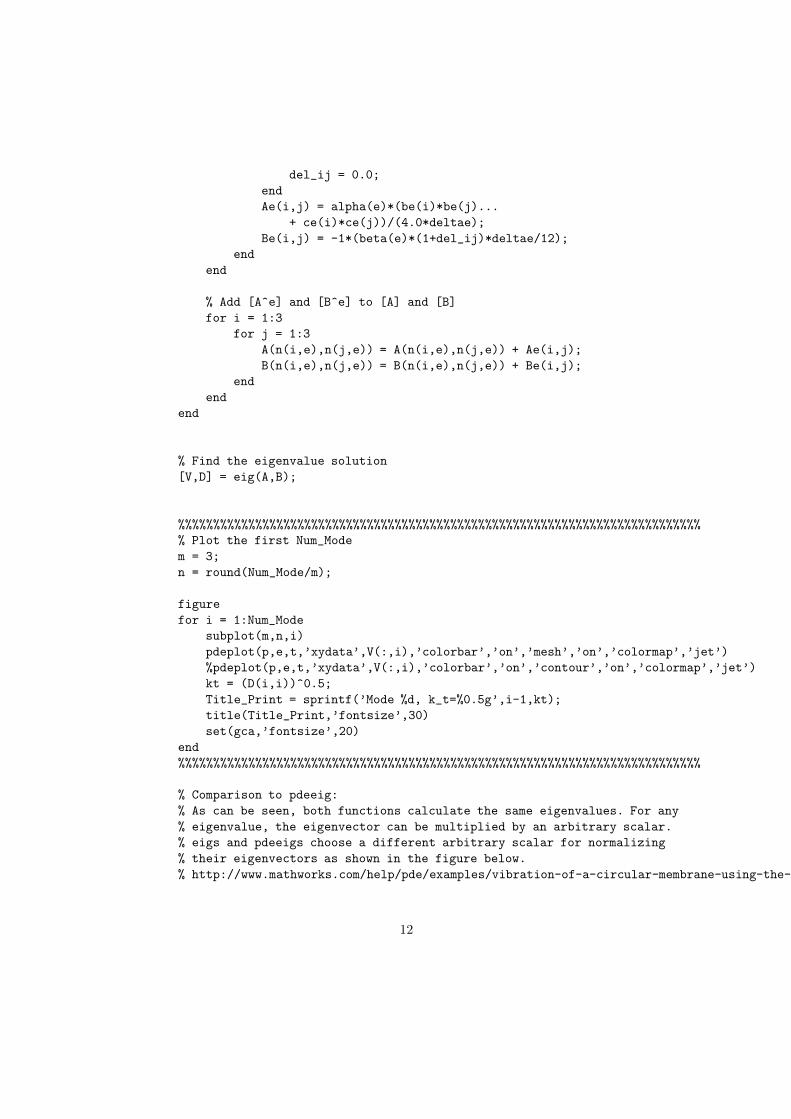
help comprise the elementary K matrix. Finally, we locate where in the largeK matrix these elemental matrices belong, given the global node numbers weassigned earlier when we created the mesh. All that remains after this, is to findthe eigenvalue solution to this matrix, and then simply plot the results usingMATLAB’s built-in commands.

3.2 Generalized Partial Differential Equation Solver Im-

plementation

After implementing our own FEM solution, we decided to verify the results usingMATLAB’s partial differential equation eigenvalue problem solving function, thecode for which can be seen in Appendix B, Subsection 2. In the first edition ofthis code, we simply output the geometry and mesh from PDEBOX (MATLAB’sGUI for solving partial differential equations), saved those as matrices, and thensolved from there. However, in the final version of the code, as you can see, wecreated the geometry matrices and mesh within the code. It’s obviously madein such a way that we can easily choose between a rectangle and circle. Wechose to refine the mesh twice, as this provided an acceptable discretization tocomputation time ratio. The boundary files are then loaded based on whetherthe simulation is using TE polarization or TM polarization, these files can beseen in Appendix B, Subsections 4 and 5. The last thing we need to do, beforeplotting the results, is to input all of the information into the MATLAB function,pdeeig. We need to provide it with the boundary conditions, point matrix forthe mesh, edge matrix for the mesh, triangle matrix for the mesh, 3 constantscorresponding to our particular differential equation, and an interval over whichto search for the eigenvalues. We already previously defined the 3 mesh matricesand the boundary conditions in the code, so we only have to define the 4 otherremaining quantities. Our eigenvalue problem is of the general form−∇·(c∇u)+au = λ(du). As was shown in class for this particular waveguide problem, c = 1,a = 0, d = 1, and λ is the eigenvalue we are looking for. Now that we have these3 constants, all that remains is the valid solution interval. Theoretically, thereare infinite eigensolutions to this problem, so we needed to limit the solutioninterval so that we could perform the calculation in a finite time. We triedvarious maximum values for k

2

t, and ended up settling on 100 as a reasonable

one for computation length, given our typical geometry size/mesh refinement.After that, we simply plot the eigenvalues/eigenvectors that were returned fromthe pdeeig function, and this gives us a solid visualization of the eigenmodes ofour waveguide, as well as their corresponding kt values.

3.3 GUI Creation

Lastly, we developed a GUI to encapsulate our solution, and make it easilyvisualized. We made the layout of the GUI using MATLAB’s GUI Design En-vironment (GUIDE). This allows you to drag and drop various buttons, menus,and axes for graphs into a window, and GUIDE will then make a figure file foryou that is exactly how you laid it out. GUIDE also creates a .m file that has

3

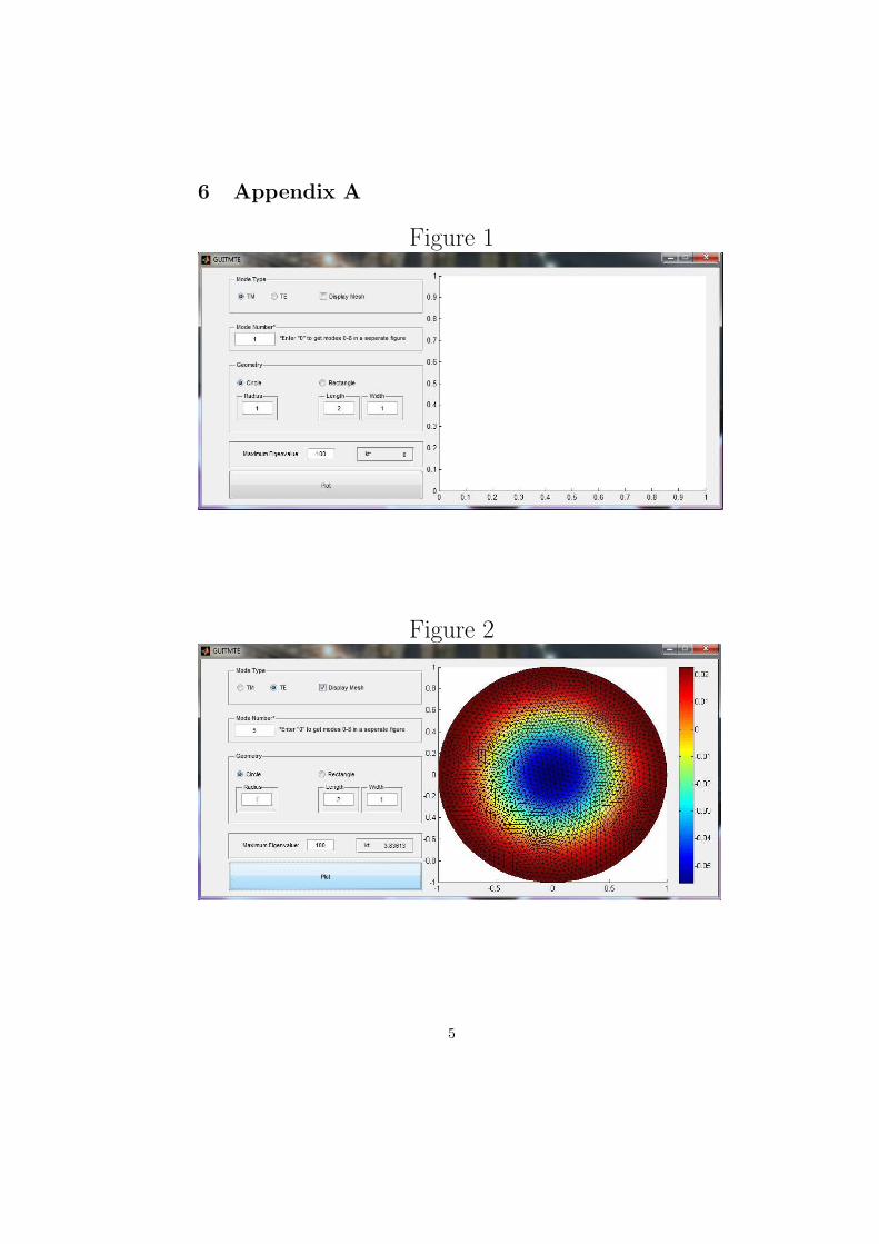
functions which execute when you click those buttons or select certain menuoptions. Within that framework, you can then easily add to those functions.You can see the code that executes when the GUI runs in Appendix B, Sub-section 3. Basically what happens, is when the user presses the “Plot” button,the program polls all the text boxes and radio buttons for their current value,and then performs the same calculation as we did with the previous pdeeig pro-gram. It then outputs the plot to the predefined axes in the MATLAB figurefor viewing, as well as the kt value. The user can also select whether they wouldlike to see the FEM mesh or the field contour when plotting, as well as providethe maximum eigenvalue they would like to attain. This lets us to refine oursearch to just the solutions they would like to see, and allows us to reduce ourcomputation time. Images of our GUI with various options selected can be seenin Appendix A, Figures 1-4.

4 Results

You can see the results that were requested in the original problem statementin Appendix A, Figures 5-9. As can be seen, these field distributions clearlymatch those we would analytically expect from a rectangular, TE waveguidewith a/b=2:1 for the first 5 modes. The values for kt in each case are alsodisplayed. We also generated the same solutions using MATLAB’s pdeeig func-tion, though the ones depicted are from our own FEM solution. For any furtherresults, please run our GUI with the desired specifications.

5 Conclusions

We have thus provided a satisfactory solution to the stated problem, as well asenabled users of our program to solve any number of other TE or TM waveg-uide problems with various geometries, namely any rectangular or circular ones.Overall, I was quite pleased with how this project turned out. We arrived at thesolutions we were hoping to, and provide, what I believe to be, a very intuitive,fast, and user-friendly GUI associated with our project. If I were to do it again,one thing I may change is to have our program calculate the first 100 modesor so of a given problem, rather than having a user guess what number they’dlike to use for maximum k

2

t. This can be a bit difficult for the user, and not

always something they actually care about. I might also add more plot optionsto the GUI so that they can display more of what they desire to see. Theseare both fairly easy inclusions if we were to want to implement them in thefuture. I learned a lot about the FEM during the course of this project, aboutbuilt-in ways in which MATLAB can solve differential equations, and about thecreation of GUIs in MATLAB. This project certainly served its purpose andhelped develop my understanding of numerical electromagnetics.

4

6 Appendix A

Figure 1

Figure 2

5

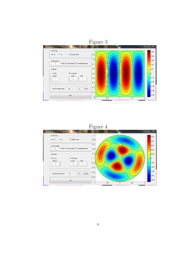
Figure 3

Figure 4

6

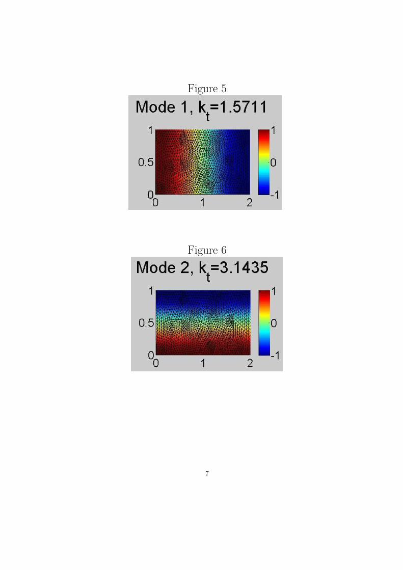
Figure 5

Figure 6

7

Figure 7

Figure 8

8

Figure 9

9

7 Appendix B

7.1 Original FEM Solution Code

%%%%%%%%%%%%%%%%%%%%%%%%%%%%%%%%%%%%%%%%%%%%%%%%%%%%%%%%%%%%%%%%n

% Brian Bentz, Dergan Lin, Andrew Velzen

% ECE 618 Project 2 - Professor Jiao

% Purdue University

%

% This program simulates the modes of an empty rectangular waveguide with

% width a and height b.

%

% 03/31/2014 - created

%%%%%%%%%%%%%%%%%%%%%%%%%%%%%%%%%%%%%%%%%%%%%%%%%%%%%%%%%%%%%%%%

close all;

clear all; clc

Num_Mode = 9; % number of modes to plot

% Define rectangle

a = 2;

b = 1;

% Create rectangle

%pderect([0 a 0 b])

gd = [3; 4; 0; a; a; 0; 0; 0; b; b]; % square geometry description matrix

g = decsg(gd);

%pdegplot(g);

% Create Mesh

[p,e,t]=initmesh(g);

[p,e,t]=refinemesh(g,p,e,t);


%pdemesh(p,e,t)

% TE case; following FEM Analysis - Sample Program (pg 169)

% Initializations to speed up code

nn = length(p); % total number of nodes

ne = length(t); % total number of elements

x = zeros(1,nn);

y = zeros(1,nn);

alpha = zeros(1,ne);

beta = zeros(1,ne);

10

n = zeros(3,ne);

%K = zeros(nn,nn);

Ae = zeros(3,3);

Be = zeros(3,3);

A = zeros(nn,nn);

B = zeros(nn,nn);

% Input data description

for i = 1:nn

x(i) = p(1,i);

y(i) = p(2,i);

end

for e = 1:ne

alpha(e) = 1;

beta(e) = -1;

%f(e) = 0;

for i = 1:3

n(i,e) = t(i,e);

end

end

% Start to assemble all area elements in Omega

for e = 1:ne

% calculate bê_i and cê_i (i = 1,2,3)

i = n(1,e);

j = n(2,e);

m = n(3,e);

be(1) = y(j) - y(m);

be(2) = y(m) - y(i);

be(3) = y(i) - y(j);

ce(1) = x(m) - x(j);

ce(2) = x(i) - x(m);

ce(3) = x(j) - x(i);

% calculate Deltaê

deltae = 0.5*(be(1)*ce(2) - be(2)*ce(1));

% generate the elemntal matricies [Kê] = [Aê] - kt^2[Bê]

% note: Be is multiplied by -1 because it is moved to the other side

% [A]{Hz}=kt^2[B]{Hz}

for i = 1:3

for j = 1:3

if i==j

del_ij = 1.0;

else

11

del_ij = 0.0;

end

Ae(i,j) = alpha(e)*(be(i)*be(j)...

+ ce(i)*ce(j))/(4.0*deltae);

Be(i,j) = -1*(beta(e)*(1+del_ij)*deltae/12);

end

end

% Add [A^e] and [B^e] to [A] and [B]

for i = 1:3

for j = 1:3

A(n(i,e),n(j,e)) = A(n(i,e),n(j,e)) + Ae(i,j);

B(n(i,e),n(j,e)) = B(n(i,e),n(j,e)) + Be(i,j);

end

end

end

% Find the eigenvalue solution

[V,D] = eig(A,B);

%%%%%%%%%%%%%%%%%%%%%%%%%%%%%%%%%%%%%%%%%%%%%%%%%%%%%%%%%%%%%%%%%%%%%%%%%%%

% Plot the first Num_Mode

m = 3;

n = round(Num_Mode/m);

figure

for i = 1:Num_Mode

subplot(m,n,i)

pdeplot(p,e,t,’xydata’,V(:,i),’colorbar’,’on’,’mesh’,’on’,’colormap’,’jet’)

%pdeplot(p,e,t,’xydata’,V(:,i),’colorbar’,’on’,’contour’,’on’,’colormap’,’jet’)

kt = (D(i,i))^0.5;

Title_Print = sprintf(’Mode %d, k_t=%0.5g’,i-1,kt);

title(Title_Print,’fontsize’,30)

set(gca,’fontsize’,20)

end

%%%%%%%%%%%%%%%%%%%%%%%%%%%%%%%%%%%%%%%%%%%%%%%%%%%%%%%%%%%%%%%%%%%%%%%%%%%

% Comparison to pdeeig:

% As can be seen, both functions calculate the same eigenvalues. For any

% eigenvalue, the eigenvector can be multiplied by an arbitrary scalar.

% eigs and pdeeigs choose a different arbitrary scalar for normalizing

% their eigenvectors as shown in the figure below.

% http://www.mathworks.com/help/pde/examples/vibration-of-a-circular-membrane-using-the-ma

12

7.2 MATLAB PDE Solution Code

%%%%%%%%%%%%%%%%%%%%%%%%%%%%%%%%%%%%%%%%%%%%%%%%%%%%%%%%%%%%%%%%



% Purdue University

%

% This program simulates the modes of an empty rectangular or circular

% waveguide with width a and height b, or radius rho.

% This program uses the MATLAB functions avaialable in the PDE

% toolbox.

%

% 04/02/2014

%%%%%%%%%%%%%%%%%%%%%%%%%%%%%%%%%%%%%%%%%%%%%%%%%%%%%%%%%%%%%%%%

close all; clear all; clc

% Define control variables (for GUI)

Rectangle = 0;

TE = 0;

a = 2;

b = 1;

rho = 1;

Eigen_mode = 0;

Mesh_flag = 0;

r_interval_max = 100; % maximum value of kt^2 computed

% Create geometry

if Rectangle

% Rectangle

%pderect([0 a 0 b])


%g = decsg(gd,’R1’);

g = decsg(gd);

%pdegplot(g);

else

% Circle

%pdecirc(0,0,rho)

gd = [1; 0; 0; rho]; % circular geometry description matrix

g = decsg(gd);

%g = decsg(gd,’C1’);

%pdegplot(g);

end

13

% Create Mesh




%pdemesh(p,e,t)

% Create boundary

if TE

bound = @boundaryFile_TEwaveguide;

type boundaryFile_TEwaveguide

else

bound = @boundaryFile_TMwaveguide;

type boundaryFile_TMwaveguide

end

% Generalized eigenvalue problem coefficients:

% Del(c Del u) + au = Lambda(du)

% eigenvalues search interval

c = 1;

a = 0;

d = 1;

r_interval = [-Inf r_interval_max];

% Solve FEM PDE eigenvalue problem

[v,l] = pdeeig(bound,p,e,t,c,a,d,r_interval);

%%%%%%%%%%%%%%%%%%%%%%%%%%%%%%%%%%%%%%%%%%%%%%%%%%%%%%%%%%%%%%%%%%%%%%%%%%%

% Plot results

if Eigen_mode

if Mesh_flag

pdeplot(p,e,t,’xydata’,v(:,Eigen_mode+1),’colorbar’,’on’,’mesh’,’on’,’colormap’,’j

else

pdeplot(p,e,t,’xydata’,v(:,Eigen_mode+1),’colorbar’,’on’,’contour’,’on’,’colormap’

end

kt = (l(Eigen_mode))^0.5;

Title_Print = sprintf(’Mode %d, k_t=%0.5g’,Eigen_mode,kt);



else

Num_Mode = 9;

m = 3;


14

figure

for i = 1:Num_Mode

subplot(m,n,i)

if Mesh_flag

pdeplot(p,e,t,’xydata’,v(:,i),’colorbar’,’on’,’mesh’,’on’,’colormap’,’jet’)

else

pdeplot(p,e,t,’xydata’,v(:,i),’colorbar’,’on’,’contour’,’on’,’colormap’,’jet’)

end

kt = (l(i))^0.5;

Title_Print = sprintf(’Mode %d, k_t=%0.5g’,i-1,kt);



end

end

%%%%%%%%%%%%%%%%%%%%%%%%%%%%%%%%%%%%%%%%%%%%%%%%%%%%%%%%%%%%%%%%%%%%%%%%%%%

7.3 GUI Creation Code

%%%%%%%%%%%%%%%%%%%%%%%%%%%%%%%%%%%%%%%%%%%%%%%%%%%%%%%%%%%%%%%%



% Purdue University

%

% 04/02/2014

%%%%%%%%%%%%%%%%%%%%%%%%%%%%%%%%%%%%%%%%%%%%%%%%%%%%%%%%%%%%%%%%

function varargout = GUITMTE(varargin)

% GUITMTE M-file for GUITMTE.fig

% GUITMTE, by itself, creates a new GUITMTE or raises the existing

% singleton*.

%

% H = GUITMTE returns the handle to a new GUITMTE or the handle to

% the existing singleton*.

%

% GUITMTE(’CALLBACK’,hObject,eventData,handles,...) calls the local

% function named CALLBACK in GUITMTE.M with the given input arguments.

%

% GUITMTE(’Property’,’Value’,...) creates a new GUITMTE or raises the

% existing singleton*. Starting from the left, property value pairs are

% applied to the GUI before GUITMTE_OpeningFcn gets called. An

% unrecognized property name or invalid value makes property application

% stop. All inputs are passed to GUITMTE_OpeningFcn via varargin.

%

% *See GUI Options on GUIDE’s Tools menu. Choose "GUI allows only one

% instance to run (singleton)".

15

%

% See also: GUIDE, GUIDATA, GUIHANDLES

% Edit the above text to modify the response to help GUITMTE

% Last Modified by GUIDE v2.5 04-Apr-2014 16:30:49

% Begin initialization code - DO NOT EDIT

gui_Singleton = 1;

gui_State = struct(’gui_Name’, mfilename, ...

’gui_Singleton’, gui_Singleton, ...

’gui_OpeningFcn’, @GUITMTE_OpeningFcn, ...

’gui_OutputFcn’, @GUITMTE_OutputFcn, ...

’gui_LayoutFcn’, [] , ...

’gui_Callback’, []);

if nargin && ischar(varargin{1})

gui_State.gui_Callback = str2func(varargin{1});

end

if nargout

[varargout{1:nargout}] = gui_mainfcn(gui_State, varargin{:});

else

gui_mainfcn(gui_State, varargin{:});

end

% End initialization code - DO NOT EDIT

% --- Executes just before GUITMTE is made visible.

function GUITMTE_OpeningFcn(hObject, eventdata, handles, varargin)

% This function has no output args, see OutputFcn.

% hObject handle to figure

% eventdata reserved - to be defined in a future version of MATLAB

% handles structure with handles and user data (see GUIDATA)

% varargin command line arguments to GUITMTE (see VARARGIN)

% Choose default command line output for GUITMTE

handles.output = hObject;

% Update handles structure

guidata(hObject, handles);

% UIWAIT makes GUITMTE wait for user response (see UIRESUME)

% uiwait(handles.figure1);

% --- Outputs from this function are returned to the command line.

function varargout = GUITMTE_OutputFcn(hObject, eventdata, handles)

16

% varargout cell array for returning output args (see VARARGOUT);

% hObject handle to figure



% Get default command line output from handles structure

varargout{1} = handles.output;

function Mode_Number_Input_Callback(hObject, eventdata, handles)

% hObject handle to Mode_Number_Input (see GCBO)



% Hints: get(hObject,’String’) returns contents of Mode_Number_Input as text

% str2double(get(hObject,’String’)) returns contents of Mode_Number_Input as a double

% --- Executes during object creation, after setting all properties.

function Mode_Number_Input_CreateFcn(hObject, eventdata, handles)

% hObject handle to Mode_Number_Input (see GCBO)


% handles empty - handles not created until after all CreateFcns called

% Hint: edit controls usually have a white background on Windows.

% See ISPC and COMPUTER.

if ispc && isequal(get(hObject,’BackgroundColor’), get(0,’defaultUicontrolBackgroundColor’

set(hObject,’BackgroundColor’,’white’);

end

% --- Executes on button press in TMrb.

function TMrb_Callback(hObject, eventdata, handles)

% hObject handle to TMrb (see GCBO)



% Hint: get(hObject,’Value’) returns toggle state of TMrb

% --- Executes on button press in TErb.

function TErb_Callback(hObject, eventdata, handles)

% hObject handle to TErb (see GCBO)



% Hint: get(hObject,’Value’) returns toggle state of TErb

17

% --- Executes on button press in Meshcb.

function Meshcb_Callback(hObject, eventdata, handles)

% hObject handle to Meshcb (see GCBO)



% Hint: get(hObject,’Value’) returns toggle state of Meshcb

% --- Executes on button press in Circlerb.

function Circlerb_Callback(hObject, eventdata, handles)

% hObject handle to Circlerb (see GCBO)



% Hint: get(hObject,’Value’) returns toggle state of Circlerb

function Radius_Input_Callback(hObject, eventdata, handles)

% hObject handle to Radius_Input (see GCBO)



% Hints: get(hObject,’String’) returns contents of Radius_Input as text

% str2double(get(hObject,’String’)) returns contents of Radius_Input as a double


function Radius_Input_CreateFcn(hObject, eventdata, handles)

% hObject handle to Radius_Input (see GCBO)







end

% --- Executes on button press in Rectanglerb.

function Rectanglerb_Callback(hObject, eventdata, handles)

% hObject handle to Rectanglerb (see GCBO)



18

% Hint: get(hObject,’Value’) returns toggle state of Rectanglerb

function Width_Input_Callback(hObject, eventdata, handles)

% hObject handle to Width_Input (see GCBO)



% Hints: get(hObject,’String’) returns contents of Width_Input as text

% str2double(get(hObject,’String’)) returns contents of Width_Input as a double


function Width_Input_CreateFcn(hObject, eventdata, handles)

% hObject handle to Width_Input (see GCBO)







end

function Length_Input_Callback(hObject, eventdata, handles)

% hObject handle to Length_Input (see GCBO)



% Hints: get(hObject,’String’) returns contents of Length_Input as text

% str2double(get(hObject,’String’)) returns contents of Length_Input as a double


function Length_Input_CreateFcn(hObject, eventdata, handles)

% hObject handle to Length_Input (see GCBO)







end

function r_Interval_edit_Callback(hObject, eventdata, handles)

19

% hObject handle to r_Interval_edit (see GCBO)



% Hints: get(hObject,’String’) returns contents of r_Interval_edit as text

% str2double(get(hObject,’String’)) returns contents of r_Interval_edit as a double


function r_Interval_edit_CreateFcn(hObject, eventdata, handles)

% hObject handle to r_Interval_edit (see GCBO)







end

function kt_Return_Callback(hObject, eventdata, handles)


function kt_Return_CreateFcn(hObject, eventdata, handles)



end

% --- Executes on button press in plot_button.

function plot_button_Callback(hObject, eventdata, handles)

% hObject handle to plot_button (see GCBO)



% Define control variables (for GUI)

% Rectangle = 0;

Rectangle = get(handles.Rectanglerb,’Value’)

% TE = 0;

TE = get(handles.TErb,’Value’)

% a = 2;

a = str2num(get(handles.Length_Input,’String’))

% b = 1;

b = str2num(get(handles.Width_Input,’String’))

% rho = 1;

rho = str2num(get(handles.Radius_Input,’String’))

20

% Eigen_mode = 0;

Eigen_mode = str2num(get(handles.Mode_Number_Input,’String’))

% Mesh_flag = 1;

Mesh_flag = get(handles.Meshcb,’Value’)

% r_interval_max = 10; % maximum value of kt^2 computed

r_interval_max = str2num(get(handles.r_Interval_edit,’String’))

% Create geometry

if Rectangle

% Rectangle

%pderect([0 a 0 b])


g = decsg(gd);

%pdegplot(g);

else

% Circle

%pdecirc(0,0,rho)

gd = [1; 0; 0; rho]; % circular geometry description matrix

g = decsg(gd);

%pdegplot(g);

end

% Create Mesh




%pdemesh(p,e,t)

% Create boundary

if TE

bound = @boundaryFile_TEwaveguide;

type boundaryFile_TEwaveguide

else

bound = @boundaryFile_TMwaveguide;

type boundaryFile_TMwaveguide

end

% Generalized eigenvalue problem coefficients:

% Del(c Del u) + au = Lambda(du)

% eigenvalues search interval

c = 1;

a = 0;

d = 1;

21

r_interval = [-Inf r_interval_max];

% Solve FEM PDE eigenvalue problem

[v,l] = pdeeig(bound,p,e,t,c,a,d,r_interval);

%%%%%%%%%%%%%%%%%%%%%%%%%%%%%%%%%%%%%%%%%%%%%%%%%%%%%%%%%%%%%%%%%%%%%%%%%%%

% Plot results

if Eigen_mode

if Mesh_flag

kt = (l(Eigen_mode+1))^0.5;

set(handles.kt_Return, ’String’, kt);

axes(handles.axes1)

pdeplot(p,e,t,’xydata’,v(:,Eigen_mode+1),’colorbar’,’on’,’mesh’,’on’,’colormap’,’j

else

kt = (l(Eigen_mode+1))^0.5;

set(handles.kt_Return, ’String’, kt);

axes(handles.axes1)

pdeplot(p,e,t,’xydata’,v(:,Eigen_mode+1),’colorbar’,’on’,’contour’,’on’,’colormap’

end

else

Num_Mode = 9;

m = 3;


figure

for i = 1:Num_Mode

subplot(m,n,i)

if Mesh_flag

pdeplot(p,e,t,’xydata’,v(:,i),’colorbar’,’on’,’mesh’,’on’,’colormap’,’jet’)

else

pdeplot(p,e,t,’xydata’,v(:,i),’colorbar’,’on’,’contour’,’on’,’colormap’,’jet’)

end

kt = (l(i))^0.5;

Title_Print = sprintf(’Mode Number: %d , k_t: %0.5g’,i-1,kt);


end

end

%%%%%%%%%%%%%%%%%%%%%%%%%%%%%%%%%%%%%%%%%%%%%%%%%%%%%%%%%%%%%%%%%%%%%%%%%%%

7.4 TE Waveguide Boundary Conditions

function [ q, g, h, r ] = boundaryFile_TEwaveguide( p, e, u, time )

%Boundary conditions for square TE waveguide

22

% returns the Neumann BC (q, g) and Dirichlet BC (h, r) matrices.

% p is the point matrix returned from INITMESH

% e is the edge matrix returned from INITMESH

% u is the solution vector (used only for nonlinear cases)

% time (used only for parabolic and hyperbolic cases)

%

% See also PDEBOUND, INITMESH

% Copyright 2012 The MathWorks, Inc.

% Modified by Brian Bentz (2014) for square TE waveguide

N = 1; % Only a single scalar PDE

ne = size(e,2);

% for TE, boundary conditions are naturally satisfied by FEM

% DelH n = 0 everywhere

q = zeros(N^2, ne);

g = zeros(N, ne);

h = zeros(N^2, 2*ne);

r = zeros(N, 2*ne);

end

7.5 TM Waveguide Boundary Conditions

function [ q, g, h, r ] = boundaryFile_TMwaveguide( p, e, u, time )

%Boundary conditions for square TE waveguide

% returns the Neumann BC (q, g) and Dirichlet BC (h, r) matrices.

% p is the point matrix returned from INITMESH

% e is the edge matrix returned from INITMESH

% u is the solution vector (used only for nonlinear cases)

% time (used only for parabolic and hyperbolic cases)

%

% See also PDEBOUND, INITMESH

% Copyright 2012 The MathWorks, Inc.

% Modified by Brian Bentz (2014) for square TE waveguide

N = 1; % Only a single scalar PDE

ne = size(e,2);

% for TM, Ez = 0 on the boundary

%

q = zeros(N^2, ne);

g = zeros(N, ne);

h = ones(N^2, 2*ne);

r = zeros(N, 2*ne);

end

23

finite element method solution of tm and te … · sibility, and the development of the gui was...

Documents