finite element methods - sccswiki · pdf filealgorithms for scientiﬁc computing finite...

Algorithms for Scientific Computing

Finite Element Methods

Michael BaderTechnical University of Munich

Summer 2016

Part I

Looking Back: Discrete Models forHeat Transfer and the Poisson

Equation

Modelling of Heat Transfer• objective: compute the temperature distribution of some object• under certain prerequisites:

• temperature T at object boundaries given• heat sources• material parameters k , . . .

• observation from physical experiments: q ≈ k · δT(heat flow proportional to temperature differences)

Michael Bader | Algorithms for Scientific Computing | Finite Element Methods | Summer 2016 2

A Finite Volume Model

• object: a rectangular metal plate (again)• model as a collection of small connected rectangular cells

hx

hy

• examine the heat flow across the cell edgesMichael Bader | Algorithms for Scientific Computing | Finite Element Methods | Summer 2016 3

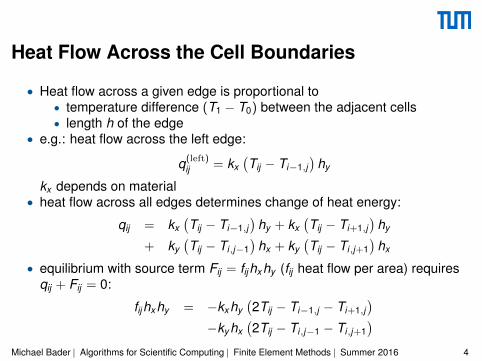
Heat Flow Across the Cell Boundaries

• Heat flow across a given edge is proportional to• temperature difference (T1 − T0) between the adjacent cells• length h of the edge

• e.g.: heat flow across the left edge:

q(left)ij = kx

(Tij − Ti−1,j

)hy

kx depends on material• heat flow across all edges determines change of heat energy:

qij = kx(Tij − Ti−1,j

)hy + kx

(Tij − Ti+1,j

)hy

+ ky(Tij − Ti,j−1

)hx + ky

(Tij − Ti,j+1

)hx

• equilibrium with source term Fij = fijhxhy (fij heat flow per area) requiresqij + Fij = 0:

fijhxhy = −kxhy(2Tij − Ti−1,j − Ti+1,j

)−ky hx

(2Tij − Ti,j−1 − Ti,j+1

)Michael Bader | Algorithms for Scientific Computing | Finite Element Methods | Summer 2016 4

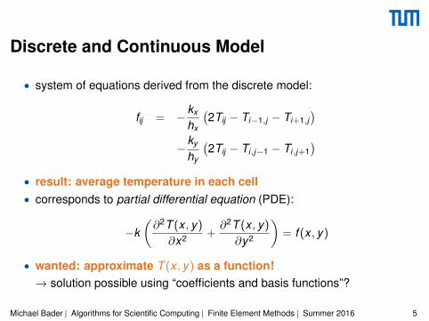
Discrete and Continuous Model

• system of equations derived from the discrete model:

fij = −kx

hx

(2Tij − Ti−1,j − Ti+1,j

)−

ky

hy

(2Tij − Ti,j−1 − Ti,j+1

)• result: average temperature in each cell• corresponds to partial differential equation (PDE):

−k(∂2T (x , y)

∂x2 +∂2T (x , y)

∂y2

)= f (x , y)

• wanted: approximate T (x , y) as a function!→ solution possible using “coefficients and basis functions”?


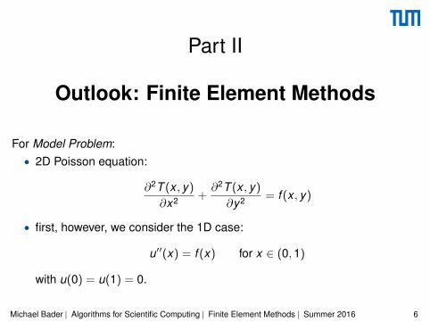
Part II

Outlook: Finite Element Methods

For Model Problem:• 2D Poisson equation:

∂2T (x , y)

∂x2 +∂2T (x , y)

∂y2 = f (x , y)

• first, however, we consider the 1D case:

u′′(x) = f (x) for x ∈ (0,1)

with u(0) = u(1) = 0.


Finite Elements – Main Idea

• we consider the residual of the (1D) PDE:

u′′(x) = f (x) u′′(x)− f (x) = 0

• represent the functions u and f in our “favorite” form:(∑ujφj (x)

)′′−∑

fjφj (x) = 0

• however: we will usually not find uj that solve this equation exactly (assolution u can not be represented as

∑ujφj (x))

• remedy?→ find “best approximation”, given by orthogonality:⟨

w(x),(∑

ujφj (x))′′−∑

fjφj (x)

⟩= 0 “for all w(x)”

• remember that < g, f >=∫

g · f dx


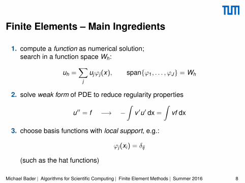
Finite Elements – Main Ingredients

1. compute a function as numerical solution;search in a function space Wh:

uh =∑

j

ujϕj (x), spanϕ1, . . . , ϕJ = Wh

2. solve weak form of PDE to reduce regularity properties

u′′ = f −→ −∫

v ′u′ dx =

∫vf dx

3. choose basis functions with local support, e.g.:

ϕj (xi ) = δij

(such as the hat functions)


Choose Test and Ansatz Space

• search for solution functions uh of the form

uh =∑

j

ujϕj (x)

• the basis (“shape”, “ansatz”) functions ϕj (x) build a vector space (orfunction space) Wh

spanϕ1, . . . , ϕJ = Wh

• the “best” solution uh in this function space is wanted


Example: Nodal Basis

ϕi (x) :=

1h (x − xi−1) xi−1 < x < xi1h (xi+1 − x) xi < x < xi+1

0 otherwise

0,60,4 0,80,20

1

1

0,4

0,2

x

0

0,8

0,6


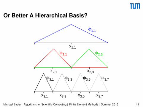
Or Better A Hierarchical Basis?

.x1,1

.

.

x2,1 x2,3

x3,1 x3,3 x3,5 x3,7

Φ1,1

Φ2,1 Φ2,3

Φ3,1 Φ3,3 Φ3,5 Φ3,7


Weak Forms and Weak Solutions

• consider a PDE Lu = f (e.g. Lu = ∆u)• transformation to the weak form:

〈v ,Lu〉 =

∫vLu dx =

∫vf dx = 〈f , v〉 ∀v ∈ V

V a certain class of functions• “real solution” u also solves the weak form

(but additional, approximate solutions accepted . . . )• motivation for weak form:

– we cannot test Lu(x) = f (x) for all x ∈ (0,1) on a computer(infinitely many x)

– frequent choice V = Wh, so check whether Lu and f have the “samebehaviour” w.r.t. scalar product

– approximate solution u might not solve PDE: Lu 6= fthus: additional functions need to be “acceptable” as solution→ “orthogonality” idea


Weak Form of the Poisson Equation – 1D

• Poisson equation with Dirichlet conditions:

−u′′(x) = f (x) in Ω = (0,1), u(0) = u(1) = 0

• weak form:−∫

Ω

v(x)u′′(x) dx =

∫Ω

v(x)f (x) dx ∀v

• integration by parts:

−∫

Ω

v(x)u′′(x) dx = −v(x) · u′(x)

∣∣∣∣10

+

∫Ω

v ′(x) · u′(x) dx

• choose functions v such that v(0) = v(1) = 0:∫Ω

v ′(x) · u′(x) dx =

∫Ω

v(x)f (x) dx ∀v


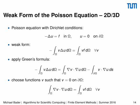
Weak Form of the Poisson Equation – 2D/3D


−∆u = f in Ω, u = 0 on δΩ

• weak form:−∫

Ω

v∆u dΩ =

∫Ω

vf dΩ ∀v

• apply Green’s formula:

−∫

Ω

v∆u dΩ =

∫Ω

∇v · ∇u dΩ−∫∂Ω

v · ∇u ds

• choose functions v such that v = 0 on ∂Ω:∫Ω

∇v · ∇u dΩ =

∫Ω

vf dΩ ∀v


Weak Form of the Poisson Equation – Summary


−∆u = f in Ω,u = 0 on δΩ

• transformed into weak form:∫Ω

∇v · ∇u dΩ =

∫Ω

vf dΩ ∀v

• weaker requirements for a solution u:twice differentiabale→ first derivative integrable

• remember use of nodal basis: availability of first vs. second derivative!


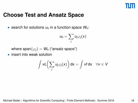
Choose Test and Ansatz Space

• search for solutions uh in a function space Wh:

uh =∑

j

ujϕj (x)

where spanϕj = Wh (“ansatz space”)• insert into weak solution∫

vL(∑

j

ujϕj (x)

)dx =

∫vf dx ∀v ∈ V


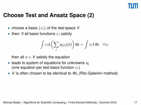
Choose Test and Ansatz Space (2)

• choose a basis ψi of the test space V• then: if all basis functions ψi satisfy∫

ψiL(∑

j

ujϕj (x)

)dx =

∫ψi f dx ∀ψi

then all v ∈ V satisfy the equation• leads to system of equations for unknowns uj

(one equation per test basis function ψi )• V is often chosen to be identical to Wh (Ritz-Galerkin method)


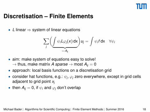
Discretisation – Finite Elements

• L linear⇒ system of linear equations∑j

(∫ψiLϕj (x) dx︸︷︷︸

=:Aij

)uj =

∫ψi f dx ∀ψi

• aim: make system of equations easy to solve!→ thus, make matrix A sparse→ most Aij = 0

• approach: local basis functions on a discretisation grid• consider hat functions, e.g.: ψj , ϕj zero everywhere, except in grid cells

adjacent to grid point xj

• then Aij = 0, if ψi and ϕj don’t overlap


Example Problem: Poisson 1D

• in 1D: u′′(x) = f (x) on Ω = (0,1),hom. Dirichlet boundary cond.: u(0) = u(1) = 0

• weak form: ∫ 1

0v ′(x) · u′(x) dx =

∫ 1

0v(x)f (x) dx ∀v

• computational grid:xi = ih, (for i = 1, . . . ,n − 1); mesh size h = 1/n

• V = W : piecewise linear functions(on intervals [xi , xi+1])


Nodal Basis

ϕi (x) :=

1h (x − xi−1) xi−1 < x < xi1h (xi+1 − x) xi < x < xi+1

0 otherwise

0,60,4 0,80,20

1

1

0,4

0,2

x

0

0,8

0,6


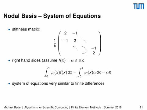
Nodal Basis – System of Equations

• stiffness matrix:

1h

2 −1

−1 2. . .

. . . . . . −1−1 2

• right hand sides (assume f (x) = α ∈ R):∫ 1

0ϕi (x)f (x) dx =

∫ 1

0ϕi (x)α dx = αh

• system of equations very similar to finite differences


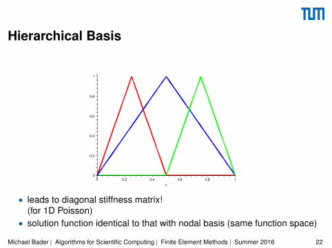
Hierarchical Basis

0,60,4 0,80,20

1

1

0,4

0,2

x

0

0,8

0,6

• leads to diagonal stiffness matrix!(for 1D Poisson)

• solution function identical to that with nodal basis (same function space)


Part III

Finite Element Methods – BasisFunctions for 2D

Hierarchical Basis in 2DQuadtrees and Hierarchical Bases

Quadtrees to Represent ObjectsHierarchical Basis vs. Quadtree


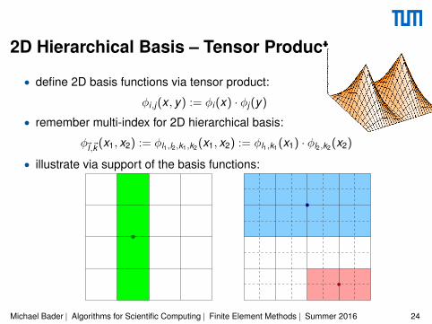
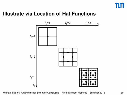
2D Hierarchical Basis – Tensor Product

• define 2D basis functions via tensor product:

φi,j (x , y) := φi (x) · φj (y)

• remember multi-index for 2D hierarchical basis:

φ~l,~k (x1, x2) := φl1,l2,k1,k2 (x1, x2) := φl1,k1 (x1) · φl2,k2 (x2)

• illustrate via support of the basis functions:


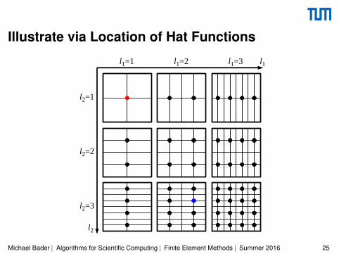
Illustrate via Location of Hat Functions

l1=1 l1=2 l1=3 l1

l2=1

l2=2

l2=3

l2


Adding Adaptivity: Quadtrees

Quadtrees to Represent Objects:

• start with an initial square (covering the entire domain)• recursive substructuring into four subsquares• adaptive refinement?


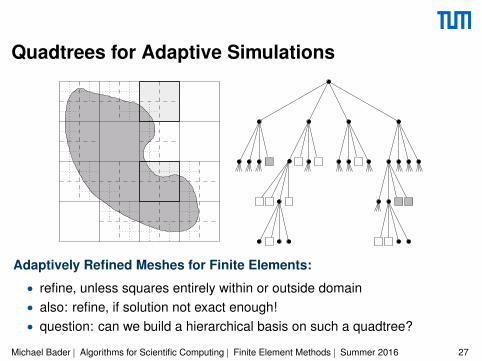
Quadtrees for Adaptive Simulations

Adaptively Refined Meshes for Finite Elements:

• refine, unless squares entirely within or outside domain• also: refine, if solution not exact enough!• question: can we build a hierarchical basis on such a quadtree?


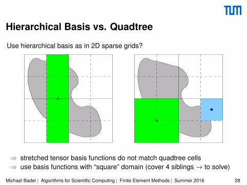
Hierarchical Basis vs. Quadtree

Use hierarchical basis as in 2D sparse grids?

⇒ stretched tensor basis functions do not match quadtree cells⇒ use basis functions with “square” domain (cover 4 siblings→ to solve)


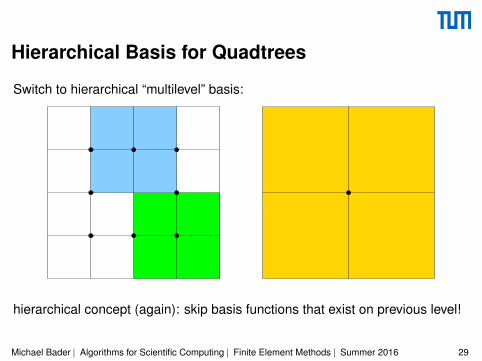
Hierarchical Basis for Quadtrees

Switch to hierarchical “multilevel” basis:

hierarchical concept (again): skip basis functions that exist on previous level!


Illustrate via Location of Hat Functions

l1=1 l1=2 l1=3 l1

l2=1

l2=2

l2=3

l2


Quadtree-Compatible Hierarchical BasisBasis Functions

Similar to tensor-product basis:• Level-wise hierarchical increments

W~l := spanφ~l,~i~i∈I~l

• Only use “diagonal” levels:

~l := l , . . . , l

• Omit grid points for which all indices areeven:

I~l := ~i : ~1 ≤~i < 2~n, any ij odd

l1=1 l1=2 l1=3 l1

l2=1

l2=2

l2=3

l2


Part IV

Finite Element Methods – TowardsImplementation

FEM and Hierarchical Basis TransformHierarchical Basis TransformationFEM and Hierarchical Basis TransformElement Stiffness MatricesWorkflow


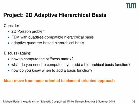
Project: 2D Adaptive Hierarchical Basis

Consider:• 2D Poisson problem• FEM with quadtree-compatible hierarchical basis• adaptive quadtree-based hierarchical basis

Discuss (again):• how to compute the stiffness matrix?• what do you need to compute, if you add a hierarchical basis function?• how do you know when to add a basis function?

Idea: move from node-oriented to element-oriented approach


Recall: Hierarchical Basis Transformation

0,60,4 0,80,20

1

1

0,4

0,2

x

0

0,8

0,6

−→

0,60,4 0,80,20

1

1

0,4

0,2

x

0

0,8

0,6

• represent “wider” hat function φ1,1(x) via basis functions φ2,j (x)

φ1,1(x) = 12φ2,1(x) + φ2,2(x) + 1

2φ2,3(x)

• consider vector of hierarchical/nodal basis functionsand write transformation as matrix-vector product:ψ2,1(x)

ψ2,2(x)ψ2,3(x)

:=

φ2,1(x)φ1,1(x)φ2,3(x)

=

1 0 012 1 1

20 0 1

φ2,1(x)φ2,2(x)φ2,3(x)


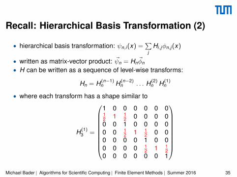
Recall: Hierarchical Basis Transformation (2)

• hierarchical basis transformation: ψn,i (x) =∑

jHi,jφn,j (x)

• written as matrix-vector product: ~ψn = Hn~φn

• H can be written as a sequence of level-wise transforms:

Hn = H(n−1)n H(n−2)

n . . . H(2)n H(1)

n

• where each transform has a shape similar to

H(1)3 =

1 0 0 0 0 0 012 1 1

2 0 0 0 00 0 1 0 0 0 00 0 1

2 1 12 0 0

0 0 0 0 1 0 00 0 0 0 1

2 1 12

0 0 0 0 0 0 1


Recall: Hierarchical Coordinate Transformation

• consider function f (x) ≈∑

iaiψn,i (x) represented via hier. basis

• wanted: corresponding representation in nodal basis∑j

bjφn,j (x) =∑

i

aiψn,i (x) ≈ f (x)

• with ψn,i (x) =∑

jHi,jφn,j (x) we obtain

∑j

bjφn,j (x) =∑

i

ai

∑j

Hi,jφn,j (x) =∑

j

∑i

aiHi,jφn,j (x)

• compare coordinates and get

bj =∑

i

Hi,jai =∑

i

(HT )

j,i ai

• written in vector notation: b = HT a


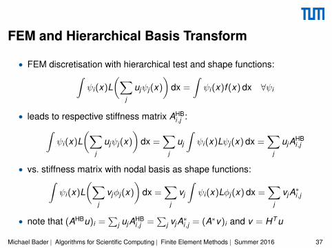
FEM and Hierarchical Basis Transform

• FEM discretisation with hierarchical test and shape functions:∫ψi (x)L

(∑j

ujψj (x)

)dx =

∫ψi (x)f (x) dx ∀ψi

• leads to respective stiffness matrix AHBi,j :∫

ψi (x)L(∑

j

ujψj (x)

)dx =

∑j

uj

∫ψi (x)Lψj (x) dx =

∑j

ujAHBi,j

• vs. stiffness matrix with nodal basis as shape functions:∫ψi (x)L

(∑j

vjφj (x)

)dx =

∑j

vj

∫ψi (x)Lφj (x) dx =

∑j

vjA∗i,j

• note that (AHBu)i =∑

j ujAHBi,j =

∑j vjA∗i,j = (A∗v)i and v = HT u


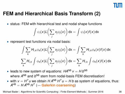
FEM and Hierarchical Basis Transform (2)

• status: FEM with hierarchical test and nodal shape functions∫ψi (x)L

(∑j

vjφj (x)

)dx =

∫ψi (x)f (x) dx

• represent test functions via nodal basis:∫ ∑k

Hi,kφk (x)L(∑

j

vjφj (x)

)dx =

∫ ∑k

Hi,kφk (x)f (x) dx

∑k

Hi,k

∫φk (x)L

(∑j

vjφj (x)

)dx =

∑k

Hi,k

∫φk (x)f (x) dx

• leads to new system of equations: HANB v = H bNB

where ANB and bNB stem from nodal-basis FEM discretisation!• with v = HT u we obtain H ANB HT u = H b as system of equations, thus:

AHB = H ANB HT ( Galerkin coarsening)


Element Stiffness Matrices

• domain Ω splitted into finite elements Ω(k):

Ω = Ω(1) ∪ Ω(2) ∪ · · · ∪ Ω(n)

• observation: basis functions are defined element-wise• use:

∫ ba f (x)dx =

∫ ca f (x)dx +

∫ bc f (x)dx

• element-wise evaluation of the integrals:∫Ω

∇v · ∇u dx =∑

k

∫Ω(k)

∇v · ∇u dx∫Ω

vf dx =∑

i

∫Ω(i)

vf dx


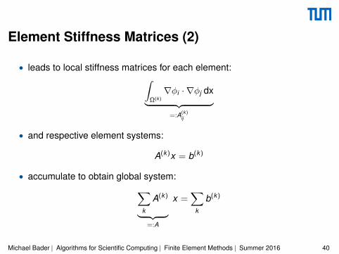
Element Stiffness Matrices (2)

• leads to local stiffness matrices for each element:∫Ω(k)

∇φi · ∇φj dx︸︷︷︸=:A(k)

ij

• and respective element systems:

A(k)x = b(k)

• accumulate to obtain global system:∑k

A(k)

︸︷︷︸=:A

x =∑

k

b(k)


Element Stiffness Matrices (3)

Some comments on notation:• assume: 1D problem, n elements (i.e. intervals)• in each element only two basis functions are non-zero!

• hence, almost all A(k)ij are zero:

A(k)ij =

∫Ω(k)

∇φi · ∇φj dx

• only 2× 2 elements of A(k) are non-zero• therefore convention to omit zero columns/rows⇒ leaves only unknowns that are in Ω(k)


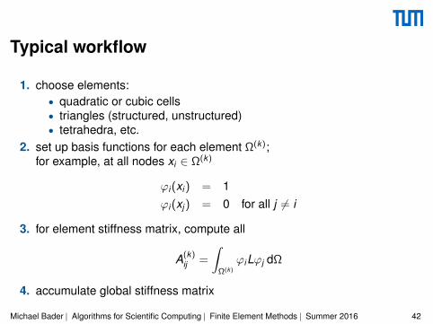
Typical workflow

1. choose elements:• quadratic or cubic cells• triangles (structured, unstructured)• tetrahedra, etc.

2. set up basis functions for each element Ω(k);for example, at all nodes xi ∈ Ω(k)

ϕi (xi ) = 1ϕi (xj ) = 0 for all j 6= i

3. for element stiffness matrix, compute all

A(k)ij =

∫Ω(k)

ϕiLϕj dΩ

4. accumulate global stiffness matrix


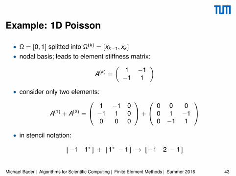
Example: 1D Poisson

• Ω = [0,1] splitted into Ω(k) = [xk−1, xk ]

• nodal basis; leads to element stiffness matrix:

A(k) =

(1 −1−1 1

)• consider only two elements:

A(1) + A(2) =

1 −1 0−1 1 00 0 0

+

0 0 00 1 −10 −1 1

• in stencil notation:

[−1 1∗ ] + [ 1∗ − 1 ] → [−1 2 − 1 ]


Project: Adaptive Hierarchical Basis

Consider:• 1D Poisson problem• FEM with hierarchical basis• however: not all basis functions used on each grid→ adaptive hierarchical basis

Discuss:• how to compute the stiffness matrix?• what do you need to compute, if you add a hierarchical basis function?• how do you know when to add a basis function?


Example: 2D Poisson

• −∆u = f on domain Ω = [0,1]2

• splitted into Ω(i,j) = [xi−1, xi ]× [xj−1, xj ]• bilinear basis functions

ϕij (x , y) = ϕi (x)ϕj (y)

• “pagoda” functions


Example: 2D Poisson (2)

• leads to element stiffness matrix:

A(k) =

2 − 1

2 − 12 −1

− 12 2 −1 − 1

2

− 12 −1 2 − 1

2

−1 − 12 − 1

2 2

• accumulation leads to 9-point stencil −1 −1 −1

−1 8 −1−1 −1 −1


finite element methods - sccswiki · pdf filealgorithms for scientiﬁc computing finite...

Documents