Heriot-Watt University Research Gateway

Heriot-Watt University

Finite-element view-factor computations for radiant energy exchangesMuneer, Tariq; Ivanova, Stoynka; Kotak, Yash Satish; Gul, Mehreen Saleem

Published in:Journal of Renewable and Sustainable Energy

DOI:10.1063/1.4921387

Publication date:2015

Document VersionPublisher's PDF, also known as Version of record

Link to publication in Heriot-Watt University Research Portal

Citation for published version (APA):Muneer, T., Ivanova, S., Kotak, Y. S., & Gul, M. (2015). Finite-element view-factor computations for radiantenergy exchanges. Journal of Renewable and Sustainable Energy, 7(3), [033108]. DOI: 10.1063/1.4921387

General rightsCopyright and moral rights for the publications made accessible in the public portal are retained by the authors and/or other copyright ownersand it is a condition of accessing publications that users recognise and abide by the legal requirements associated with these rights.

If you believe that this document breaches copyright please contact us providing details, and we will remove access to the work immediatelyand investigate your claim.

Download date: 13. Jun. 2018

Finite-element view-factor computations for radiant energy exchangesT. Muneer, S. Ivanova, Y. Kotak, and M. Gul Citation: Journal of Renewable and Sustainable Energy 7, 033108 (2015); doi: 10.1063/1.4921387 View online: http://dx.doi.org/10.1063/1.4921387 View Table of Contents: http://scitation.aip.org/content/aip/journal/jrse/7/3?ver=pdfcov Published by the AIP Publishing Articles you may be interested in Influence of thermal energy on exchange-bias studied by finite-element simulations Appl. Phys. Lett. 103, 042410 (2013); 10.1063/1.4816664 Numerical Study on Radiative Heat Transfer and Boundary Control of Glass Fibers Cooling Process AIP Conf. Proc. 1262, 155 (2010); 10.1063/1.3482224 Transient Temperature Distribution Analysis at an Orthotropic Metal Bar by Finite Element Method AIP Conf. Proc. 1244, 196 (2010); 10.1063/1.3462760 Finite Element Analysis of Cross‐Wedge Rolling Process AIP Conf. Proc. 1252, 747 (2010); 10.1063/1.3457630 A Finite Element Model for the Thermal Transport in Solid Targets AIP Conf. Proc. 915, 983 (2007); 10.1063/1.2750939

This article is copyrighted as indicated in the article. Reuse of AIP content is subject to the terms at: http://scitation.aip.org/termsconditions. Downloaded to IP:

137.195.8.130 On: Wed, 01 Jul 2015 15:17:01

Finite-element view-factor computations for radiant energyexchanges

T. Muneer,1,a) S. Ivanova,2,a) Y. Kotak,3,b) and M. Gul3,a)

1Edinburgh Napier University, 10 Colinton Road, EH10 5DT Edinburgh, United Kingdom2University of Architecture, Civil Engineering and Geodesy, Sofia, Bulgaria3Heriot-Watt University, EH14 4AS Edinburgh, United Kingdom

(Received 23 March 2015; accepted 3 May 2015; published online 19 May 2015)

Radiation heat transfer has very many applications within the building services sector.

CIBSE (Chartered Institution of Building Services Engineers) Guide A provides the

physics background and the relevant mathematical functions for radiant energy

exchanges between surfaces of different configurations in chapters 2 and 5. The aim

of this article is to present procedures for inter-surface radiant energy exchange that

range from the most simple (macro-) to most general formulations that are based on a

micromesh, finite-element approach. The justification for such detailed procedures

and their applicability within the modern building energy simulation software is also

covered. VC 2015 AIP Publishing LLC. [http://dx.doi.org/10.1063/1.4921387]

I. INTRODUCTION

In any given society buildings in general have been identified to be one of the most energy

consuming sector. Within the EU28, it has been reported1 that buildings are responsible for

over 50% of the gross energy budget. Furthermore, the bulk of the above proportion of energy

use may be attributed to heating or cooling of buildings.

There has been a demand by the respective national governments to address the above

issue of such large-scale energy consumption and numerous legislation related instruments were

introduced to encourage energy efficiency. The building services community has responded to

the above challenge and one of the positive actions undertaken was refining of building energy

simulation tools. As a result, over the past few decades, the software tools have evolved from

being part-physics, part-empirical to tools that use the physical laws in a more fundamental

manner. Examples that may be cited here are Computational Fluid Dynamics (CFD) tools for

solving air-flow problems and daylighting software such as RADIANCE.

CFD simulation software allows to predict the impact of fluid flow on any product through-

out the design and manufacturing as well as during end use. It works on the phenomena like

studying single or multiphase, isothermal or reacting, compressible or not by giving valuable

insight into product performance.

RADIANCE software is used for the analysis and visualization of lightning design. The

primary advantage of this software is there are no limitations on the geometry or to materials

that may be simulated. It is used by architects and engineers to predict illumination, visual

quality, and appearance of innovative design space and by researchers to evaluate new lightning

and daylight technologies.

In a recent publication, the present research team has presented a case for obtaining build-

ing cooling load profile from a numerical solution of the fundamental heat conduction equa-

tion.2 Another example that may be cited here is the work of Laccarino et al. (2010)3 who

developed a building energy model that coupled a CFD tool with heat transfer information

from an energy simulation tool. Their intention was to produce an integrated CFD-energy

a)T. Muneer, S. Ivanova, and M. Gul contributed equally to this work.b)Author to whom correspondence should be addressed. Electronic mail: yk78@hw.ac.uk.

1941-7012/2015/7(3)/033108/20/$30.00 VC 2015 AIP Publishing LLC7, 033108-1

JOURNAL OF RENEWABLE AND SUSTAINABLE ENERGY 7, 033108 (2015)

This article is copyrighted as indicated in the article. Reuse of AIP content is subject to the terms at: http://scitation.aip.org/termsconditions. Downloaded to IP:

137.195.8.130 On: Wed, 01 Jul 2015 15:17:01

simulation model. Their model was then validated using data from monitored buildings in

California. The above report is also available at Stanford University.4

The above-mentioned, recursive and computer-intensive developments have only been pos-

sible due to the exponential rise of computing power and its cost reduction. A brief review of

the latter would therefore be not out of order at this stage.

The highest performing computing machines that are currently in use hundreds of thou-

sands of processing cores and are capable of 1015 (petaflop) floating point operations per sec-

ond. That is a thousand times more than the most powerful machine of 2000, which in turn

were a thousand times more than a decade before that.

Researchers associated with the U.S. Government Sandia Advance Devices Technologies

laboratory5 have assessed that today’s (2014) desktop computing cost of 181MFlops/$ will drop

to 18GFlops/$ by the year 2030. The average current microprocessor clock speeds would also

increase to 33 GHz by the year 2015. For supercomputers the main demand for increasing com-

puting speed is from the climate change modelling community. However, the building energy

simulation would benefit from such developments. The Edinburgh-based supercomputing facil-

ity6 is forecasting an increase of computing power from today’s Petflops to Exaflops by year

2020 while Sandia’s researchers are predicting a performance of the order of Zettaflops (1021)

for the year 2030.

However, there are certain challenges that lie ahead. It is being predicted that the high per-

formance exascale computing machines will have different architectures from that which has

dominated for the last decade and more. There will be an impact on software; existing software

will most likely need to be rewritten.7 Therefore, in brief, due to increased computing power that is

now available at ever decreasing cost there is a general trend towards the incorporation of fundamen-

tal physical laws and processes, rather than use of empiricism within building energy simulation

tools. Within the Chartered Institution of Building Services Engineers Guides design charts related to

radiation exchange between surfaces that are either parallel or perpendicular to each other are pre-

sented. Those charts are somewhat restrictive though and do not allow for estimation of energy

exchange for surfaces facing each other at an acute or obtuse angle. Furthermore, the issue of ground-

reflected radiation that is incident upon tilted solar thermal and photovoltaic (PV) collectors has not

been addressed within existing literature appropriately. On occasions, there are also incidences where

radiation reflected off any given building’s glass facade is of interest. An interesting example that

may be cited herein is that of a new London skyscraper that has been blamed for reflecting light

which melted parts of a car parked on a nearby street.8 One of the present research team members

was asked to provide preliminary advice regarding analysis of that problem.

To summarise, therefore, there are at least two areas of applicability of radiation energy

exchange for the proposed work:

(i) sol-air temperature and building cooling load due to energy exchange from ground and

neighbouring building surfaces;

(ii) energy balance of solar thermal collectors and PV modules, once again taking into account

the ground-reflected solar radiation.

The aim of this article is to present procedures for inter-surface radiant energy exchange

that range from the most simple (macro-) to most general formulations that are based on a

micromesh, finite-element approach.

II. ANALYSIS

A. Radiation exchange between any two surfaces

For any two black surfaces, the thermal radiation exchange is given by the following equation:

Q1�2 ¼ rðT14 � T2

4ÞA1F1�2 ¼ rðT24 � T1

4ÞA2F2�1: (1)

Within heat transfer terminology the term F1–2 is known as “configuration factor” (CF).9

There are also other names for the latter such as “view factor,” “geometry factor,” “angle

033108-2 Muneer et al. J. Renewable Sustainable Energy 7, 033108 (2015)

This article is copyrighted as indicated in the article. Reuse of AIP content is subject to the terms at: http://scitation.aip.org/termsconditions. Downloaded to IP:

137.195.8.130 On: Wed, 01 Jul 2015 15:17:01

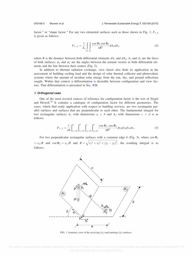
factor,” or “shape factor.” For any two elemental surfaces such as those shown in Fig. 1, F1–2

is given as follows:

F1�2 ¼1

A1

ðA1

ðA2

cos U1 cos U2

pR2dA2dA1; (2)

where R is the distance between both differential elements dA1 and dA2; A1 and A2 are the faces

of both surfaces; /1 and /2 are the angles between the normal vectors to both differential ele-

ments and the line between their centres (Fig. 2).

In addition to thermal radiation exchange, view factor also finds its application in the

assessment of building cooling load and the design of solar thermal collector and photovoltaic

systems where the amount of incident solar energy from the sun, sky, and ground reflections

sought. Within that context a differentiation is desirable between configuration and view fac-

tors. That differentiation is presented in Sec. II B.

1. Orthogonal case

One of the most revered sources of reference for configuration factor is the text of Siegel

and Howell.10 It contains a catalogue of configuration factor for different geometries. The

cases, which find ready application with respect to building services, are two rectangular par-

allel surfaces and surfaces that are perpendicular to each other. The fundamental integral for

two rectangular surfaces A1 with dimensions a � b and A2 with dimensions c � d is as

follows:

F1�2 ¼1

ab

ða

x1¼0

ðb

y1¼0

ðc

x2¼0

ðd

y2¼0

cos U1: cos U2

pR2dy2dx2dy1dx1: (3)

For two perpendicular rectangular surfaces with a common edge b (Fig. 3), where cos U1

¼ x2=R and cos U2 ¼ x1=R and R ¼ffiffiffiffiffiffiffiffiffiffiffiffiffiffiffiffiffiffiffiffiffiffiffiffiffiffiffiffiffiffiffiffiffiffiffiffiffiffiffiffiffiffiffiffix1

2 þ x22 þ ðy1 � y2Þ2

q, the resulting integral is as

follows:

FIG. 1. Isometric view of the receiving (A1) and emitting (A2) surfaces.

033108-3 Muneer et al. J. Renewable Sustainable Energy 7, 033108 (2015)

This article is copyrighted as indicated in the article. Reuse of AIP content is subject to the terms at: http://scitation.aip.org/termsconditions. Downloaded to IP:

137.195.8.130 On: Wed, 01 Jul 2015 15:17:01

F1�2 ¼1

ab

ða

x1¼0

ðb

y1¼0

ðc

x2¼0

ðb

y2¼0

x1x2

p x12 þ x2

2 þ y1 � y2ð Þ2h i2

dy2dx2dy1dx1: (4)

The configuration factor, solution of this integral, is as follows, where N¼ c/b and L¼ a/b:

F1�2¼1

pL

Ltan–1 1

L

� �þNtan–1 1

N

� ��

ffiffiffiffiffiffiffiffiffiffiffiffiffiffiffiN2þL2p

tan–1 1ffiffiffiffiffiffiffiffiffiffiffiffiffiffiffiN2þL2p� �

þ1

4ln

1þL2ð Þ 1þN2ð Þ1þL2þN2

� �þL2ln

L2 1þN2þL2ð Þ1þL2ð Þ 1þN2ð Þ

" #þN2ln

N2 1þN2þL2ð Þ1þN2ð Þ N2þL2ð Þ

" #( )0BBBB@

1CCCCA:

(5)

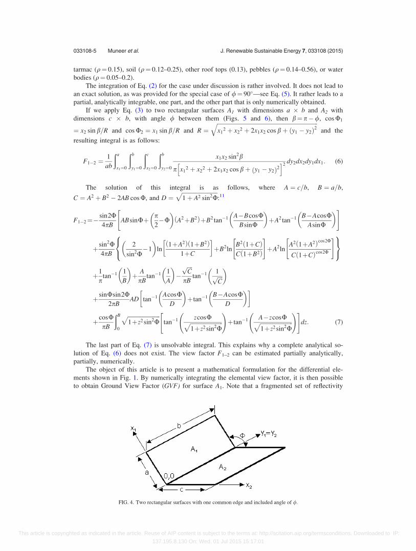
2. Tilted surface

A more generalised version of the above case is however the one where the two surfaces

A1 and A2 are not perpendicular to each other. Rather, they are separated by any given angle /that may or may not be 90�, as shown in Fig. 4.

This generalised case, once again, has a number of applications such as solar energy

reflected off ground and incident on a sloping roof, solar thermal water or air collectors, or

indeed photovoltaic modules. Note that for any given situation the ground reflected radiation may

emanate from a conglomeration of surfaces of disparate reflectivities such as grass (q¼ 0.24),

FIG. 2. Defining geometry for configuration factor.9

FIG. 3. Two orthogonal surfaces with one common edge.

033108-4 Muneer et al. J. Renewable Sustainable Energy 7, 033108 (2015)

This article is copyrighted as indicated in the article. Reuse of AIP content is subject to the terms at: http://scitation.aip.org/termsconditions. Downloaded to IP:

137.195.8.130 On: Wed, 01 Jul 2015 15:17:01

tarmac (q¼ 0.15), soil (q¼ 0.12–0.25), other roof tops (0.13), pebbles (q¼ 0.14–0.56), or water

bodies (q¼ 0.05–0.2).

The integration of Eq. (2) for the case under discussion is rather involved. It does not lead to

an exact solution, as was provided for the special case of /¼ 90�—see Eq. (5). It rather leads to a

partial, analytically integrable, one part, and the other part that is only numerically obtained.

If we apply Eq. (3) to two rectangular surfaces A1 with dimensions a � b and A2 with

dimensions c � b, with angle / between them (Figs. 5 and 6), then b¼ p�/, cos U1

¼ x2 sin b=R and cos U2 ¼ x1 sin b=R and R ¼ffiffiffiffiffiffiffiffiffiffiffiffiffiffiffiffiffiffiffiffiffiffiffiffiffiffiffiffiffiffiffiffiffiffiffiffiffiffiffiffiffiffiffiffiffiffiffiffiffiffiffiffiffiffiffiffiffiffiffiffiffiffiffiffiffiffiffiffiffiffiffix1

2 þ x22 þ 2x1x2 cos bþ ðy1 � y2Þ2

qand the

resulting integral is as follows:

F1�2 ¼1

ab

ða

x1¼0

ðb

y1¼0

ðc

x2¼0

ðb

y2¼0

x1x2 sin2b

p x12 þ x2

2 þ 2x1x2 cos bþ y1 � y2ð Þ2h i2

dy2dx2dy1dx1: (6)

The solution of this integral is as follows, where A ¼ c=b, B ¼ a=b,

C ¼ A2 þ B2 � 2AB cos U, and D ¼ffiffiffiffiffiffiffiffiffiffiffiffiffiffiffiffiffiffiffiffiffiffiffiffiffi1þ A2 sin2U

p:11

F1�2¼�sin2U4pB

ABsinUþ p2�U

� �A2þB2ð ÞþB2 tan�1 A�BcosU

BsinU

� �þA2 tan�1 B�AcosU

AsinU

� �" #

þ sin2U4pB

2

sin2U�1

� �ln

1þA2ð Þ 1þB2ð Þ1þC

� �þB2ln

B2 1þCð ÞC 1þB2ð Þ

" #þA2ln

A2 1þA2ð Þcos2U

C 1þCð Þcos2U

" #8<:

9=;

þ1

ptan�1 1

B

� �þ A

pBtan�1 1

A

� ��

ffiffiffiffiCp

pBtan�1 1ffiffiffiffi

Cp� �

þ sinUsin2U2pB

AD tan�1 AcosUD

� �þ tan�1 B�AcosU

D

� �� �

þcosUpB

ðB

0

ffiffiffiffiffiffiffiffiffiffiffiffiffiffiffiffiffiffiffiffiffiffiffi1þz2 sin2U

ptan�1 zcosUffiffiffiffiffiffiffiffiffiffiffiffiffiffiffiffiffiffiffiffiffiffiffi

1þz2 sin2Up

!þ tan�1 A�zcosUffiffiffiffiffiffiffiffiffiffiffiffiffiffiffiffiffiffiffiffiffiffiffi

1þz2 sin2Up

!" #dz: (7)

The last part of Eq. (7) is unsolvable integral. This explains why a complete analytical so-

lution of Eq. (6) does not exist. The view factor F1–2 can be estimated partially analytically,

partially, numerically.

The object of this article is to present a mathematical formulation for the differential ele-

ments shown in Fig. 1. By numerically integrating the elemental view factor, it is then possible

to obtain Ground View Factor (GVF) for surface A1. Note that a fragmented set of reflectivity

FIG. 4. Two rectangular surfaces with one common edge and included angle of /.

033108-5 Muneer et al. J. Renewable Sustainable Energy 7, 033108 (2015)

This article is copyrighted as indicated in the article. Reuse of AIP content is subject to the terms at: http://scitation.aip.org/termsconditions. Downloaded to IP:

137.195.8.130 On: Wed, 01 Jul 2015 15:17:01

data for the foreground (surface A2) can be easily handled in this approach, an example of

which is presented towards the end of thus article. Furthermore, a Visual Basic for Application

(VBA) code is presented that would enable the reader to obtain the GVF for any given geome-

try and choice of reflectivities for the foreground (surface A2).

B. Comparison and difference between configuration factor and view factor

CF: The configuration factor Fi�j is defined as the fraction of diffusely radiated energy

leaving surface Ai that is incident on surface Aj. It is estimated with Eq. (2).

The configuration factor Fi�j participates in the product Ai.Fi�j.Ii that reflects the energy flux

uniformly emitted from surface Ai to surface Aj. There Ii is the value of the emitted irradiance from

surface i. From the view point of surface Aj, the product Aj.Fj�i.Ii is the energy flux received by sur-

face Aj from uniformly emitting surface Ai. Even from different viewpoints, both expressions esti-

mate the same flux of energy and this easily leads to a reciprocity relation between both factors.

By above definition Fi�j means that surface Ai is emitting, surface Aj is receiving, thus the

configuration factor Fi�j is “viewing” from the position of the emitting surface Ai. In other words,

Fi�j represents how well the surface Ai sees surface Aj and explains why Fi�j is not equal to Fj�i.

In building facade energy exchange we usually need “viewing” from the position of the

receiving surface. This is why the definitions and values of the configuration factor and from

other side Sky View Factor (SVF) and GVF are different.

FIG. 5. Projection of A1 and A2 surfaces on the X2/Y and X2/Z planes.

FIG. 6. Detail of projection X2/Z plane.

033108-6 Muneer et al. J. Renewable Sustainable Energy 7, 033108 (2015)

This article is copyrighted as indicated in the article. Reuse of AIP content is subject to the terms at: http://scitation.aip.org/termsconditions. Downloaded to IP:

137.195.8.130 On: Wed, 01 Jul 2015 15:17:01

SVF: By definition, SVF is the ratio of the sky radiation received by a surface A to the radia-

tion emitted by the entire sky hemispheric environment. In other words, SVF represents how well

the surface sees the sky hemisphere. The approach presumes that the sky hemisphere is uniformly

emitting. The concept is applied in the estimation of the background diffuse irradiance on a sur-

face, although the diffuse radiance actually has an anisotropic nature. On the other hand, the

approach is suitable to be used in the estimation of building heat loss through radiation to the sky

hemisphere. The relationship between SVF and CF is given by the following equation:

SVF ¼ CFðAREAemitting=AREAreceivingÞ: (8)

GVF is the ratio of the reflected ground radiation received by a planar surface to radiation

emitted by the entire hemispheric ground environment. The widely used isotropic constant

model (ICM) of Liu and Jordan12 for estimation of the reflected irradiance assumes a constant

albedo and needs a GVF, which we can estimate from the value of CF as follows:

GVF ¼ CFðAREAemitting=AREAreceivingÞ: (9)

The reflected irradiance Ii depends on the global horizontal irradiance IGH and the albedo

q—as follows:

Ii ¼ qIGH: (10)

The total reflected radiation RR received by the surface Aj from the uniform reflecting sur-

face Ai is estimated with the following equation:

RR ¼ qIGHAiFi�j ¼ qIGHAjFj�i ¼ qIGHAjGVF: (11)

If we need to study the 2D-variations in the incident irradiance, it is better to use the third

variant of this equation: RR ¼ qIGHAjGVF.

C. View factor algebra

The view factor algebra is a combination of basic configuration factors between surfaces

with different geometries and some fundamental relations between them:9

• Superposition rules: Two superposition rules could be defined for the view factors to surfaces.

They help to estimate the view factors which cannot be evaluated directly.

Rule 1: The product of the view factor Fi�j from a surface i to surface j and the area Ai of sur-

face i is equal to the sum of the products of the view factors from the parts of surface i to sur-

face j and their areas,

Fi�jAi ¼XN

k¼1

Fik�jAik : (12)

Rule 2: The view factor Fi�j from a surface i to surface j is equal to the sum of the view fac-

tors from the surface i to the parts of the surface j,

Fi�j ¼XN

k¼1

Fi�jk : (13)

• Summation rule: The sum of the view factors from a given surface in an enclosure, including

the possible self-view factor for concave surfaces, is 1.• Reciprocity relation: A reciprocity relation between two opposite view factors of two isotropic

emitting/receiving surfaces exists and allows the calculation of a view factor from the knowl-

edge of its reciprocal

033108-7 Muneer et al. J. Renewable Sustainable Energy 7, 033108 (2015)

This article is copyrighted as indicated in the article. Reuse of AIP content is subject to the terms at: http://scitation.aip.org/termsconditions. Downloaded to IP:

137.195.8.130 On: Wed, 01 Jul 2015 15:17:01

AiFi�j ¼ AjFj�i: (14)

• Bounding: View factors are bounded to 0�Fi�j� 1 by definition.

New derivative view factors can be computed from a set of known factors with the help of

the mentioned fundamental relations. Let us check this possibility with some exemplary

configurations.

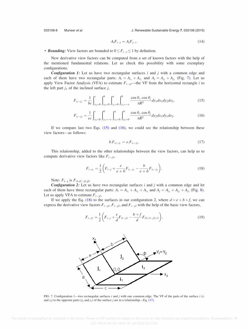
Configuration 1: Let us have two rectangular surfaces i and j with a common edge and

each of them have two rectangular parts: Ai ¼ Ai1 þ Ai2 and Aj ¼ Aj1 þ Aj2 (Fig. 7). Let us

apply View Factor Analysis (VFA) to estimate Fi�j1—the VF from the horizontal rectangle i to

the left part j1 of the inclined surface j,

Fi2�j1 ¼1

bc

ðc

x2¼0

ðb

y2¼0

ða

x1¼0

ð0

y1¼�e

cos hi: cos hj

pR2dy1dx1dy2dx2; (15)

Fi1�j2 ¼1

ec

ðc

x2¼0

ð0

y1¼�e

ða

x1¼0

ðb

y2¼0

cos hi: cos hj

pR2dy2dx1dy1dx2: (16)

If we compare last two Eqs. (15) and (16), we could see the relationship between these

view factors—as follows:

b:Fi2�j1 ¼ e:Fi1�j2 : (17)

This relationship, added to the other relationships between the view factors, can help us to

compute derivative view factors like Fi�j1,

Fi�j1 ¼1

2Fi�j þ

e

eþ bFi1�j1 �

b

eþ bFi2�j2

� �: (18)

Note: Fi�j is Fi1,i2�j1,j2.

Configuration 2: Let us have two rectangular surfaces i and j with a common edge and let

each of them have three rectangular parts: Ai ¼ Ai1 þ Ai2 þ Ai3 and Aj ¼ Aj1 þ Aj2 þ Aj3 (Fig. 8).

Let us apply VFA to estimate Fi�j2.

If we apply the Eq. (18) to the surfaces in our configuration 2, where d¼ eþ bþ f, we can

express the derivative view factors Fi�j1, Fi�j2, and Fi�j3 with the help of the basic view factors,

Fi�j1 ¼1

2Fi�j þ

e

dFi1�j1 �

bþ f

dFi2þ3�j2þ3

� �; (19)

FIG. 7. Configuration 1—two rectangular surfaces i and j with one common edge. The VF of the parts of the surface i (i1and i2) to the opposite parts (j2 and j1) of the surface j are in a relationship—Eq. (17).

033108-8 Muneer et al. J. Renewable Sustainable Energy 7, 033108 (2015)

This article is copyrighted as indicated in the article. Reuse of AIP content is subject to the terms at: http://scitation.aip.org/termsconditions. Downloaded to IP:

137.195.8.130 On: Wed, 01 Jul 2015 15:17:01

Fi�j3 ¼1

2Fi�j þ

f

dFi3�j3 �

eþ b

dFi1þ2�j1þ2

� �; (20)

Fi�j2 ¼1

2deþ bð ÞFi1þ2�j1þ2 þ bþ fð ÞFi2þ3�j2þ3 � fFi3�j3 � eFi1�j1

� �: (21)

If j2 is the receiving surface, the derivative view factor Fj2�i is more useful,

Fj2�i ¼1

2beþ bð ÞFj1þ2�i1þ2 þ bþ fð ÞFj2þ3�i2þ3 � fFj3�i3 � eFj1�i1

� �: (22)

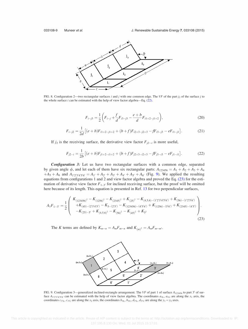
Configuration 3: Let us have two rectangular surfaces with a common edge, separated

by given angle /, and let each of them have six rectangular parts: A123456 ¼ A1 þ A2 þ A3 þ A4

þA5 þ A6 and A102030405060 ¼ A10 þ A20 þ A30 þ A40 þ A50 þ A60 (Fig. 9). We applied the resulting

equations from configurations 1 and 2 and view factor algebra and proved the Eq. (23) for the esti-

mation of derivative view factor F1–30 for inclined receiving surface, but the proof will be omitted

here because of its length. This equation is presented in Ref. 13 for two perpendicular surfaces,

A1F1�30 ¼1

2

K123456ð Þ2 � K

1256ð Þ2 � K2345ð Þ2 þ K

25ð Þ2 � K 4;5;6ð Þ� 102030405060ð Þ þ K 56ð Þ� 10205060ð Þ

þK 45ð Þ� 20304050ð Þ � K5� 2050ð Þ � K 123456ð Þ� 405060ð Þ þ K 1256ð Þ� 5060ð Þ þ K 2345ð Þ� 4050ð Þ

�K 25ð Þ�50 þ K 4;5;6ð Þ2 � K56ð Þ2 � K

45ð Þ2 þ K52

0BB@

1CCA:(23)

The K terms are defined by Km�n ¼ AmFm�n and KðmÞ2 ¼ AmFm�m0 .

FIG. 8. Configuration 2—two rectangular surfaces i and j with one common edge. The VF of the part j2 of the surface j to

the whole surface i can be estimated with the help of view factor algebra—Eq. (22).

FIG. 9. Configuration 3—generalized inclined-rectangle arrangement. The VF of part 1 of surface A123456 to part 30 of sur-

face A102030405060 can be estimated with the help of view factor algebra. The coordinates a1L, a1U are along the x1 axis, the

coordinates c30L, c30U are along the x2 axis, the coordinates b1L, b1U, d30L, d30U are along the y1¼ y2 axes.

033108-9 Muneer et al. J. Renewable Sustainable Energy 7, 033108 (2015)

This article is copyrighted as indicated in the article. Reuse of AIP content is subject to the terms at: http://scitation.aip.org/termsconditions. Downloaded to IP:

137.195.8.130 On: Wed, 01 Jul 2015 15:17:01

D. Derivation of a numerically integrable, general purpose GVF

If we consider the rectangular surfaces Ai and Aj with a common edge b as composed of

many very small rectangular areas (Fig. 10(a)), we could use numeric integration to receive the

same result with a small loss of accuracy,

Fj�i ¼sin2U

p:Na:Nb

XNa

j1¼1

XNb

j2¼1

XNc

i1¼1

XNb

i2¼1

xixj

xi2 þ xj

2 � 2xixj cos Uþ yi � yjð Þ2h i2

DcDb; (24)

where Da¼ a/Na, Db¼ b/Nb, Dc¼ c/Nc, and Na, Nb, Nc are the numbers of intervals for the

numeric integration in each dimension. The coordinates of each fragment’s center are: for surface

i� xi¼ (i1� 0.5)Dc; yi¼ (i2� 0.5)Db; for surface j� xj¼ (j1� 0.5)Da; and yj¼ (j2� 0.5)Db. Such

solution has one main significant advantage—it easily can be adapted for any disposition of both

rectangular surfaces (Fig. 10(b)), but also has two serious disadvantages—it gives an approximate

result and to avoid this with large numbers of intervals, it needs a lot of computing time.

In case of non-uniform reflectivities of the reflecting surface (Fig. 11), such approach is

irreplaceable. Let us divide the non-uniform reflecting rectangular surface in an orthogonal grid

and to estimate the average albedo value for each cell of this grid. The GVF from surface Aj to

ground surface Ai, corrected with the albedo values, is given by the following equation:

F0j�i ¼sin2Upab

XNa

j1¼1

XNb

j2¼1

XNc

i1¼1

XNd

i2¼1

xixjqi

xi2 þ xj

2 � 2xixj cos Uþ yi � yjð Þ2h i2

DaDbDcDd: (25)

Two interesting studies by Walton14,15 are dedicated to the numerical calculation of radia-

tion view factors between plane convex polygons with obstructions. In the first work,14 he

found that Gaussian integration (quadrature) improves the accuracy of the numerical integration.

This means that the function is evaluated at specially selected points instead of uniformly dis-

tributed points. Such non-uniform spacing can also be used in evaluating area integrals. In Sec.

FIG. 10. The reflecting and receiving surfaces are divided in two directions to receive a regular perpendicular grid: (a) both

surfaces have one common edge and (b) both surfaces are non-intersecting.

FIG. 11. Case with a non-uniform reflecting surface: (a) both surfaces have one common edge and (b) both surfaces are

non-intersecting.

033108-10 Muneer et al. J. Renewable Sustainable Energy 7, 033108 (2015)

This article is copyrighted as indicated in the article. Reuse of AIP content is subject to the terms at: http://scitation.aip.org/termsconditions. Downloaded to IP:

137.195.8.130 On: Wed, 01 Jul 2015 15:17:01

III, we will describe our experience and results with improved accuracy when a non-uniform

spacing is used for numerical contour integration.

III. COMPUTATIONAL TOOL DEVELOPMENT

In the present work, using Eqs. (24) and (25), four sets of numerically integrating codes

were developed to obtain GVF. These four codes represent the evolution of the present work

and demonstrate the code architecture from being simple-most and yet of low efficiency to

highly efficient but more complex. Those cases are:

A. Uniform grid

A uniform grid, where all cells within the emitting plane are of same dimension and aspect

ratio, is applied on the reflecting surface. Likewise, the cells within the receiving plane have

similar properties. The lengths of cells within the emitting and receiving planes may or may

not be equal. Square grids for both surfaces show better accuracy in the estimating of VF. This

approach can be easily applied as on a combination of two surfaces with one common edge

(Fig. 10(a)), as on a combination of two non-intersecting rectangular surfaces that are inclined

to each other (Fig. 10(b)). For square cells the total number of cells on the receiving surface is

Nreceiving_cells¼ (b/a).Na2, and the total number of iterations is Nreceiving_cells.Nemitting_cells. This

approach does not allow to reach a high accuracy for surfaces, where size a is 10 or more times

less than sizes b and c. On the other hand, it is easy to be expanded to deal with a non-uniform

reflectivity.

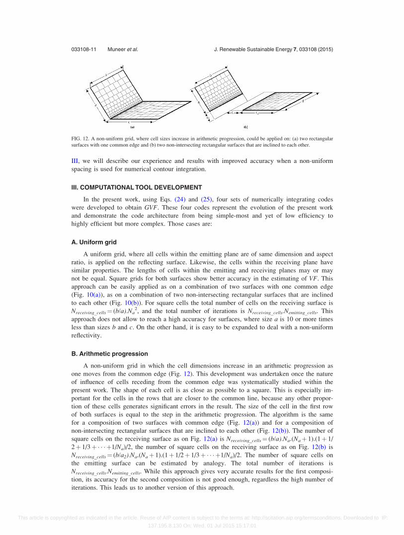
B. Arithmetic progression

A non-uniform grid in which the cell dimensions increase in an arithmetic progression as

one moves from the common edge (Fig. 12). This development was undertaken once the nature

of influence of cells receding from the common edge was systematically studied within the

present work. The shape of each cell is as close as possible to a square. This is especially im-

portant for the cells in the rows that are closer to the common line, because any other propor-

tion of these cells generates significant errors in the result. The size of the cell in the first row

of both surfaces is equal to the step in the arithmetic progression. The algorithm is the same

for a composition of two surfaces with common edge (Fig. 12(a)) and for a composition of

non-intersecting rectangular surfaces that are inclined to each other (Fig. 12(b)). The number of

square cells on the receiving surface as on Fig. 12(a) is Nreceiving_cells¼ (b/a).Na.(Naþ 1).(1þ 1/

2þ 1/3þ � � � þ1/Na)/2, the number of square cells on the receiving surface as on Fig. 12(b) is

Nreceiving_cells¼ (b/a2).Na.(Naþ 1).(1þ 1/2þ 1/3þ � � � þ1/Na)/2. The number of square cells on

the emitting surface can be estimated by analogy. The total number of iterations is

Nreceiving_cells.Nemitting_cells. While this approach gives very accurate results for the first composi-

tion, its accuracy for the second composition is not good enough, regardless the high number of

iterations. This leads us to another version of this approach.

FIG. 12. A non-uniform grid, where cell sizes increase in arithmetic progression, could be applied on: (a) two rectangular

surfaces with one common edge and (b) two non-intersecting rectangular surfaces that are inclined to each other.

033108-11 Muneer et al. J. Renewable Sustainable Energy 7, 033108 (2015)

This article is copyrighted as indicated in the article. Reuse of AIP content is subject to the terms at: http://scitation.aip.org/termsconditions. Downloaded to IP:

137.195.8.130 On: Wed, 01 Jul 2015 15:17:01

C. Proportional arithmetic progression

The analysis of the accuracy for the previous approach for non-intersecting rectangular surfa-

ces shows that cell size and number of cells in a row have to be in relation to the distance from the

common line of both planes and to increase slowly. It is suitable the size of cells in first row to be

equal to the step in the arithmetic progression only when the surface is adjoining to the common

edge (Figs. 13(a) and 13(b)), else the cells in the first row need to have bigger size, proportional to

its distance from the common line of both planes (Figs. 13(c) and 13(d)). The first step is to esti-

mate the number of virtual rows Na0 in the interval between the common line of both planes and

the lower edge of the receiving surface. The number of square cells on a receiving surface as on

Fig. 13(a) is the same as for the previous approach. The number of square cells on the receiving

surface on Fig. 13(c) is Nreceiving_cells¼ [b/(a1þ a2)]. (NaþNa0).(NaþNa0þ 1).[1/(Na0þ 1)þ 1/

(Na0þ 2)þ� � �þ1/(Na0þNa)]/2. The number of square cells on the emitting surface can be esti-

mated by analogy. The total number of iterations is Nreceiving_cells.Nemitting_cells.

It is interesting to see that this approach with lower number of considered cells and itera-

tions gives better results than the previous approach. The conclusion is the bigger numbers of

cells (iterations) does not always mean better accuracy. It is important where the grid is more

close-meshed and how much in comparison with other parts of the surface. Last two approaches

are especially better in comparison with uniform grid approach for surfaces, where size a is 10

or more times less than sizes b and c.

More details and a pictorial comparison of last two algorithms are given on Figs. 14 and

15 with a flow-diagram for the cell generation. In Sec. IV, the above three procedures for cell

generation shall be validated using data and examples presented by earlier researchers.

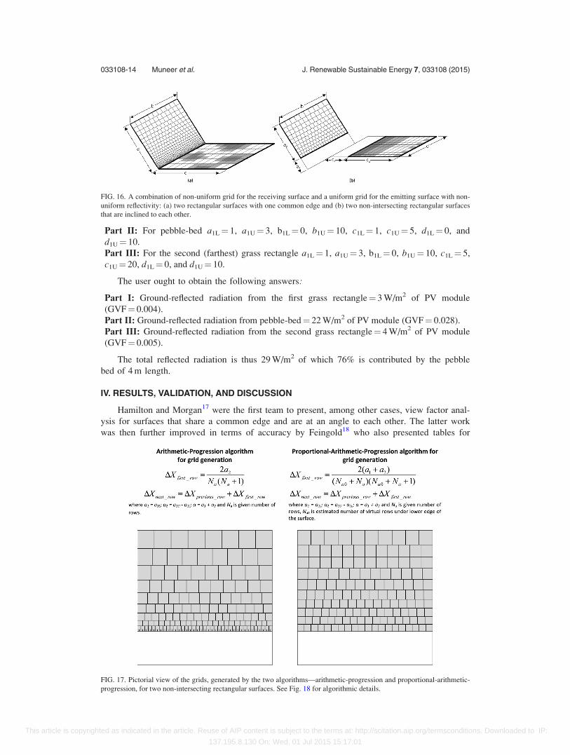
D. Combined approach

The proportional-arithmetic-progression approach is suitable to be applied on a receiving sur-

face. On other hand, sometimes it is difficult to be applied on the non-uniform emitting surface,

where the regular grid is more convenient. A combined approach can unite the advantages of both

approaches (high accuracy and easy preparing of the foreground albedo matrix) and to decrease their

FIG. 13. A non-uniform grid, where cells increase in a proportional arithmetic progression, could be applied on (a) two rec-

tangular surfaces with one common edge; (b) grid for receiving surface with Na¼ 20 rows of cells; (c) two non-intersecting

rectangular surfaces that are inclined to each other; and (d) grid for receiving surface with Na¼ 10 rows of cells.

033108-12 Muneer et al. J. Renewable Sustainable Energy 7, 033108 (2015)

This article is copyrighted as indicated in the article. Reuse of AIP content is subject to the terms at: http://scitation.aip.org/termsconditions. Downloaded to IP:

137.195.8.130 On: Wed, 01 Jul 2015 15:17:01

disadvantages (Fig. 16). The resulting number of iterations and corresponding computer time will be

lower than for the previous two approaches, based only on irregular grids.

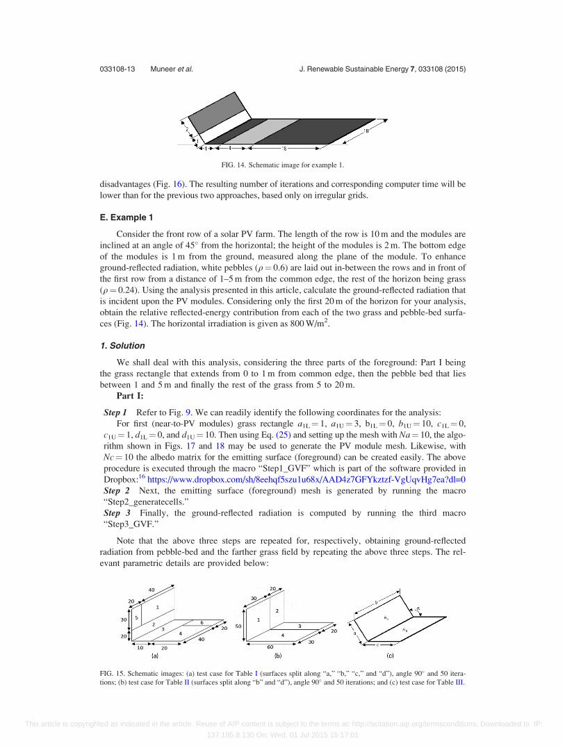
E. Example 1

Consider the front row of a solar PV farm. The length of the row is 10 m and the modules are

inclined at an angle of 45� from the horizontal; the height of the modules is 2 m. The bottom edge

of the modules is 1 m from the ground, measured along the plane of the module. To enhance

ground-reflected radiation, white pebbles (q¼ 0.6) are laid out in-between the rows and in front of

the first row from a distance of 1–5 m from the common edge, the rest of the horizon being grass

(q¼ 0.24). Using the analysis presented in this article, calculate the ground-reflected radiation that

is incident upon the PV modules. Considering only the first 20 m of the horizon for your analysis,

obtain the relative reflected-energy contribution from each of the two grass and pebble-bed surfa-

ces (Fig. 14). The horizontal irradiation is given as 800 W/m2.

1. Solution

We shall deal with this analysis, considering the three parts of the foreground: Part I being

the grass rectangle that extends from 0 to 1 m from common edge, then the pebble bed that lies

between 1 and 5 m and finally the rest of the grass from 5 to 20 m.

Part I:

Step 1 Refer to Fig. 9. We can readily identify the following coordinates for the analysis:

For first (near-to-PV modules) grass rectangle a1L¼ 1, a1U¼ 3, b1L¼ 0, b1U¼ 10, c1L¼ 0,

c1U¼ 1, d1L¼ 0, and d1U¼ 10. Then using Eq. (25) and setting up the mesh with Na¼ 10, the algo-

rithm shown in Figs. 17 and 18 may be used to generate the PV module mesh. Likewise, with

Nc¼ 10 the albedo matrix for the emitting surface (foreground) can be created easily. The above

procedure is executed through the macro “Step1_GVF” which is part of the software provided in

Dropbox:16 https://www.dropbox.com/sh/8eehqf5szu1u68x/AAD4z7GFYkztzf-VgUqvHg7ea?dl=0

Step 2 Next, the emitting surface (foreground) mesh is generated by running the macro

“Step2_generatecells.”

Step 3 Finally, the ground-reflected radiation is computed by running the third macro

“Step3_GVF.”

Note that the above three steps are repeated for, respectively, obtaining ground-reflected

radiation from pebble-bed and the farther grass field by repeating the above three steps. The rel-

evant parametric details are provided below:

FIG. 14. Schematic image for example 1.

FIG. 15. Schematic images: (a) test case for Table I (surfaces split along “a,” “b,” “c,” and “d”), angle 90� and 50 itera-

tions; (b) test case for Table II (surfaces split along “b” and “d”), angle 90� and 50 iterations; and (c) test case for Table III.

033108-13 Muneer et al. J. Renewable Sustainable Energy 7, 033108 (2015)

This article is copyrighted as indicated in the article. Reuse of AIP content is subject to the terms at: http://scitation.aip.org/termsconditions. Downloaded to IP:

137.195.8.130 On: Wed, 01 Jul 2015 15:17:01

Part II: For pebble-bed a1L¼ 1, a1U¼ 3, b1L¼ 0, b1U¼ 10, c1L¼ 1, c1U¼ 5, d1L¼ 0, and

d1U¼ 10.

Part III: For the second (farthest) grass rectangle a1L¼ 1, a1U¼ 3, b1L¼ 0, b1U¼ 10, c1L¼ 5,

c1U¼ 20, d1L¼ 0, and d1U¼ 10.

The user ought to obtain the following answers:

Part I: Ground-reflected radiation from the first grass rectangle¼ 3 W/m2 of PV module

(GVF¼ 0.004).

Part II: Ground-reflected radiation from pebble-bed¼ 22 W/m2 of PV module (GVF¼ 0.028).

Part III: Ground-reflected radiation from the second grass rectangle¼ 4 W/m2 of PV module

(GVF¼ 0.005).

The total reflected radiation is thus 29 W/m2 of which 76% is contributed by the pebble

bed of 4 m length.

IV. RESULTS, VALIDATION, AND DISCUSSION

Hamilton and Morgan17 were the first team to present, among other cases, view factor anal-

ysis for surfaces that share a common edge and are at an angle to each other. The latter work

was then further improved in terms of accuracy by Feingold18 who also presented tables for

FIG. 16. A combination of non-uniform grid for the receiving surface and a uniform grid for the emitting surface with non-

uniform reflectivity: (a) two rectangular surfaces with one common edge and (b) two non-intersecting rectangular surfaces

that are inclined to each other.

FIG. 17. Pictorial view of the grids, generated by the two algorithms—arithmetic-progression and proportional-arithmetic-

progression, for two non-intersecting rectangular surfaces. See Fig. 18 for algorithmic details.

033108-14 Muneer et al. J. Renewable Sustainable Energy 7, 033108 (2015)

This article is copyrighted as indicated in the article. Reuse of AIP content is subject to the terms at: http://scitation.aip.org/termsconditions. Downloaded to IP:

137.195.8.130 On: Wed, 01 Jul 2015 15:17:01

view factors for surfaces with a common edge and inclined to each other at various angles. The

above two works of reference have been catalogued by Siegel and Howell10 who also provide

software for obtaining view factor. The limitation however with the latter is that the solution

can only be obtained for inclined planes that meet at a common edge. Furthermore, the solution

is obtained through an analytical route, thus limiting its use when an irregular horizon with

varying reflectivity is provided. In the present work, a numerical solution is obtained using a

finite-element grid which is capable of handling an irregular horizon. The reflectivity data may

be provided via a two-dimensional table (see the example file provided on this web address16).

Also presented in this work is the analytical solution for view factor between two non-

intersecting surfaces that are inclined to each other (see Eq. (23) and Fig. 9).

With the view to validate the present software, developed within the MS-Excel environ-

ment using a VBA tool, Tables I–III have been prepared. The estimated values with our

FIG. 18. Computational flow diagram for generating the grid using proportional-arithmetic-progression procedure.

033108-15 Muneer et al. J. Renewable Sustainable Energy 7, 033108 (2015)

This article is copyrighted as indicated in the article. Reuse of AIP content is subject to the terms at: http://scitation.aip.org/termsconditions. Downloaded to IP:

137.195.8.130 On: Wed, 01 Jul 2015 15:17:01

numerical approach were compared with values, received with the analytical approach,

described in Secs. II A–II C and validated with calculated data, published by Holman,13 Siegel

and Howell,10 Hamilton and Morgan,17 Feingold,18 and Suryanarayana.19

The chosen view factors are to demonstrate the flexibility of the software to handle inte-

grated- or split surfaces with equal ease. Examples of the former (integrated) case that may be

cited are the radiant energy exchange between two walls that have a common edge, or a solar

collector (thermal or PV module) that receives ground-reflected energy. An example of the lat-

ter (split surface) may be a window within a room that is exchanging energy with walls or

ceiling.

Note that in all cases presented within Tables I and II the difference between the analytical

and numerical solution is under 0.055%. The accuracy figures for Table III exceed 99.9%. If,

however, a higher accuracy is required then the number of iterations may be increased. Note

also that for surfaces that are at an acute angle to each other (see case 1 within Table III), a

slightly higher grid resolution is required to achieve appropriate accuracy.

The structure of the software is of a general nature and it thus enables incorporation of

other cases for planer radiant view factor evaluation.

Refer to Table IV which has been prepared to inter-compare the performance of four cur-

rently developed cell-generation algorithms. In the top half of this table, the accuracy of three

algorithms is presented. To enable a direct comparison between the algorithms a scoring system

has been presently developed. This scoring system, referred as Time-Error-Product (TEP), ena-

bles algorithmic evaluation, i.e., a low score is sought. The “Combined” algorithm outperforms

the “Uniform” and “Arithmetic Progression” algorithms, respectively, by factors of 22 and 5.

Note that for any given geometry when a common edge is shared between the emitting and

receiving surfaces the two algorithms, i.e., “Arithmetic Progression” and “Proportional

Arithmetic Progression” converge and hence the top half of Table IV only contains the three

given algorithms. The lower half of Table IV also presents a comparison of all four algorithms,

TABLE I. Evaluation and validation of the numerical model with combined grid: Test case 1—Fig. 15(a)—surfaces split

along “a,” “b,” “c,” and “d,” Na¼ 50, Nc¼ 50, Nd¼ 50, angle 90�. Sub-cases 1, 3, 5, and 7 are based on17 and compared

with the results there.

Number Sub case GVF numeric GVF analytic No. of iterations Error (%) Timea (s)

1 F2–4,6 0.12279722 0.12277560 43 102 500 0.018 59

2 F1–4,6 0.07002322 0.07001912 8 552 500 0.006 12

3 F2–3,4,6 0.29747763 0.29740258 43 102 500 0.025 59

4 F1,5–3 0.01586171 0.01586182 12 790 000 �0.001 17

5 F1,5,2–3,4,6 0.16921932 0.16917600 17 282 500 0.026 24

6 F5–6 0.00763796 0.00763791 4 305 000 0.001 7

7 F2–3a 0.17470547 0.17462698 43 102 500 0.045 59

8 F2–3b 0.17470547 0.17462698 43 102 500 0.001 62

aTime for execution on a laptop with 5 GB RAM and 2.67 GHz Intel Core I5 processor.bTime for execution on a desktop with 4 GB RAM and 3 GHz Intel Core Duo processor.

TABLE II. Evaluation and validation of the numerical model with combined grid: Test case 2—Fig. 15(b)—surfaces split

along “b” and “d,” Na¼ 50, Nc¼ 50, Nd¼ 50, angle 90�. All sub-cases are based on Ref. 17 and compared with the results

there.

Number Sub-case GVF numeric GVF analytic No. of iterations Error (%) Time (s)

1 F1,2–3,4 0.21117310 0.21116258 14 412 500 0.005 20

2 F1–4 0.17025320 0.17027844 8 672 500 �0.015 12

3 F2–3 0.13803786 0.13809616 5 810 000 �0.042 8

4 F1–3 0.04482170 0.04479754 8 672 500 0.054 12

5 F2–4 0.06722647 0.06719631 5 810 000 0.045 8

033108-16 Muneer et al. J. Renewable Sustainable Energy 7, 033108 (2015)

This article is copyrighted as indicated in the article. Reuse of AIP content is subject to the terms at: http://scitation.aip.org/termsconditions. Downloaded to IP:

137.195.8.130 On: Wed, 01 Jul 2015 15:17:01

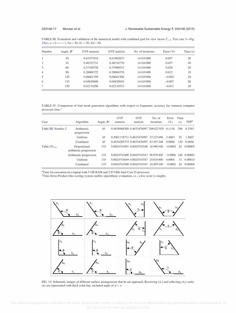
TABLE III. Evaluation and validation of the numerical model with combined grid for view factor F1–2: Test case 3—Fig.

15(c), a¼ b¼ c¼ 1, Na¼ 50, Nc¼ 50, Nd¼ 50.

Number Angle, U� GVF numeric GVF analytic No. of iterations Error (%) Time (s)

1 30 0.61937934 0.61902833 14 410 000 0.057 20

2 45 0.48352731 0.48334770 14 410 000 0.037 20

3 60 0.37100758 0.37090532 14 410 000 0.028 20

4 90 0.20006725 0.20004378 14 410 000 0.012 19

5 120 0.08661359 0.08661500 14 410 000 �0.002 20

6 135 0.04830608 0.04830945 14 410 000 �0.007 20

7 150 0.02134296 0.02134533 14 410 000 �0.011 20

TABLE IV. Comparison of four mesh generation algorithms with respect to fragments, accuracy for common computer

processor time.a

Case Algorithm Angle, U�GVF

numeric

GVF

analytic

No. of

iterations

Error

(%)

Time

(s) TEPb

Table III, Number 2 Arithmetic

progression

45 0.4838968388 0.4833476997 208 022 929 0.1136 296 0.3363

Uniform 45 0.5001118731 0.4833476997 33 223 696 3.4683 45 1.5607

Combined 45 0.4834285373 0.4833476997 83 307 248 0.0006 120 0.0696

Table I F5–6 Proportional

arithmetic progression

135 0.0024743491 0.0024743546 16 996 540 �0.0002 24 0.00005

Arithmetic progression 135 0.0024743400 0.0024743547 96 978 400 �0.0006 140 0.00083

Uniform 135 0.0024743649 0.0024743547 24 010 000 0.0004 33 0.00014

Combined 135 0.0024743508 0.0024743547 16 459 100 �0.0002 24 0.00004

aTime for execution on a laptop with 5 GB RAM and 2.67 GHz Intel Core I5 processor.bTime-Error-Product (this scoring system enables algorithmic evaluation, i.e., a low score is sought).

FIG. 19. Schematic images of different surface arrangements that fit our approach. Receiving (A1) and reflecting (A2) surfa-

ces are represented with thick solid line, included angle of /<p.

033108-17 Muneer et al. J. Renewable Sustainable Energy 7, 033108 (2015)

This article is copyrighted as indicated in the article. Reuse of AIP content is subject to the terms at: http://scitation.aip.org/termsconditions. Downloaded to IP:

137.195.8.130 On: Wed, 01 Jul 2015 15:17:01

but for the two surfaces being split, i.e., without a common edge. In this case the performance

of “Combined” and “Proportional Arithmetic Progression” algorithms nearly converge. They

are both, however, much more efficient than the “Uniform” and “Arithmetic Progression” mod-

els outperforming them by a factor of 5 and 20, respectively (see the final column that provides

the TEP figures).

The present set of numerical algorithms can easily handle radiation exchange problems

where the emitting surface has a non-uniform grid of reflectivities. Many examples of non-

uniform horizon of solar energy collection systems may be cited. In this respect, the following

web links will illustrate the point under discussion.20–24 Example 1 presented in Sec. III E is an

illustration of the latter subject. Other schematic images of different surface arrangements that

fit our approach are presented on Figs. 19–21. Many of them could be related with different

reflecting and receiving surfaces in urban canyons.

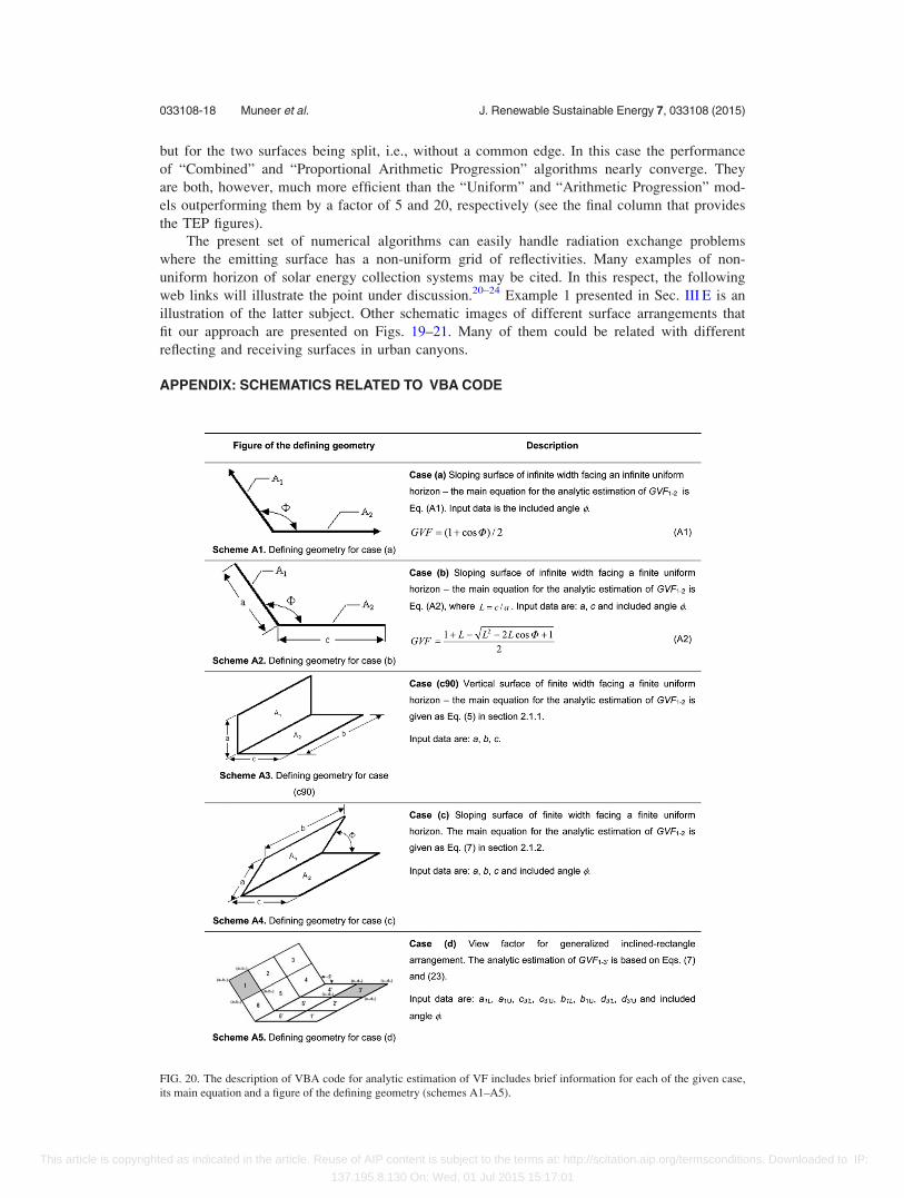
APPENDIX: SCHEMATICS RELATED TO VBA CODE

FIG. 20. The description of VBA code for analytic estimation of VF includes brief information for each of the given case,

its main equation and a figure of the defining geometry (schemes A1–A5).

033108-18 Muneer et al. J. Renewable Sustainable Energy 7, 033108 (2015)

This article is copyrighted as indicated in the article. Reuse of AIP content is subject to the terms at: http://scitation.aip.org/termsconditions. Downloaded to IP:

137.195.8.130 On: Wed, 01 Jul 2015 15:17:01

1A. Hirsch, S. Pless, R. Guglielmetti, and P. A. Torcellini, The Role of Modeling When Designing for Absolute EnergyUse Intensity Requirements in a Design-Build Framework, see http://www.nrel.gov/sustainable_nrel/pdfs/49067.pdf

2S. C. M. Hui, Energy performance of air-conditioned buildings in Hong Kong, Ph.D. thesis, 1996, Chap. 6: BuildingEnergy Simulation Methods, City University of Hong Kong, available at http://web.hku.hk/~cmhui/thesis/chp6.pdf

3G. Laccarino, M. Fischer, and E. Hult, Towards Improved Energy Simulation Tools for Buildings: Improving AirflowParameterizations Within Energy Simulation Using CFD and Building Measurements, June 22 2010, see http://www.ies-ve.com/content/mediaassets/pdf/p135final-long.pdf

4G. Iaccarino, M. Fischer, and E. Hult, Towards Improved Energy Simulation Tools for Buildings. Improving AirflowParameterizations Within Energy Simulation Using CFD and Building Measurements, see http://www.stanford.edu/group/peec/cgi-bin/docs/buildings/research/Improved%20Energy%20Simulation%20Tools%20for%20Buildings.pdf

5See http://intelligence.org/2014/04/03/erik-debenedictis/ for Erik DeBenedictis on supercomputing.6See http://www.planethpc.eu/index.php?option=com_content&view¼article&id=48 for High Performance ComputingFAQ.

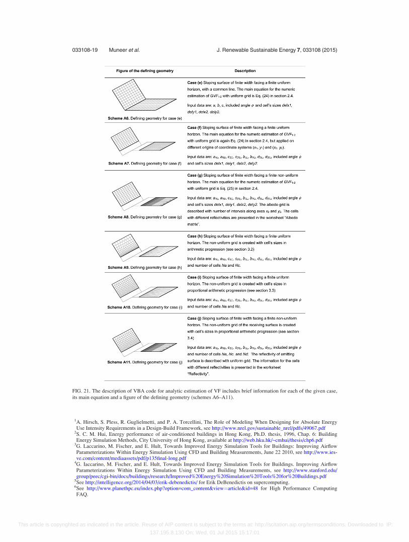
FIG. 21. The description of VBA code for analytic estimation of VF includes brief information for each of the given case,

its main equation and a figure of the defining geometry (schemes A6–A11).

033108-19 Muneer et al. J. Renewable Sustainable Energy 7, 033108 (2015)

This article is copyrighted as indicated in the article. Reuse of AIP content is subject to the terms at: http://scitation.aip.org/termsconditions. Downloaded to IP:

137.195.8.130 On: Wed, 01 Jul 2015 15:17:01

7The Future of Computing Performance: Game Over or Next Level?, Committee on Sustaining Growth in ComputingPerformance, edited by S. H. Fuller and L. I. Millett (National Research Council, Washington DC, 2011).

8See http://www.bbc.com/news/uk-england-london-23930675 for BBC NEWS London: “Walkie-Talkie” skyscraper meltsJaguar car parts.

9J. R. Howell, A Catalog of Radiation Heat Transfer - Configuration Factors, Introduction, see http://www.thermalradia-tion.net/intro.html

10R. Siegel and J. Howell, Thermal Radiation and Heat Transfer, 4th ed. (Taylor & Francis, New York, 2002).11J. R. Howell, A Catalog of Radiation Heat Transfer - Configuration Factors, C-16: Two Rectangles With One Common

Edge and Included Angle of U, see http://www.thermalradiation.net/sectionc/C-16.html12B. Y. H. Liu and R. C. Jordan, “The long term average performance of flat plate solar energy collectors,” Sol. Energy 7,

53–74 (1963).13J. P. Holman, Heat Transfer, 7th ed. (McGraw-Hill, New York, 1992).14G. N. Walton, Algorithms for Calculating Radiation View Factors Between Plane Convex Polygons With Obstructions,

National Bureau of Standards (NBSIR 86-3463), 1987 - shortened report in Fundamentals and Applications of RadiationHeat Transfer (American Society of Mechanical Engineers, 1986), HTD-Vol.72.

15G. N. Walton, “Calculation of obstructed view factors by adaptive integration,” Technical Report No. NISTIR–6925,National Institute of Standards and Technology (NIST), Gaithersburg, MD, 2002.

16See https://www.dropbox.com/sh/8eehqf5szu1u68x/AAD4z7GFYkztzf-VgUqvHg7ea?dl¼0 for VBA code for numericalcomputation of view factor for inclined surfaces: available on: https://www.dropbox.com/sh/8eehqf5szu1u68x/AAD4z7GFYkztzf-VgUqvHg7ea?dl=0.

17D. C. Hamilton and W. R. Morgan, “Radiant Interchange Configuration Factors,” Technical Note 2836, NationalAdvisory Committee for Aeronautics, Washington D.C., 1952.

18A. Feingold, “Radiant interchange configuration factors between various selected plane surfaces,” Proc. R. Soc. London,Ser. A 292(1428), 51–60 (1966).

19N. V. Suryanarayana, Engineering Heat Transfer (West Publishing Company, New York, 1995).20See http://www.photon.info/photon_news_detail_en.photon?id¼87696 for solar’s economics ensure it will be an essential

part of the world’s future energy mix, Citigroup, August, 2014.21D. Roberts, Energy Democracy: Three Ways to Bring Solar Power to the Masses, 2012, see http://www.motherearth-

news.com/renewable-energy/community-solar-energy-zwfz1209zhun.aspx#axzz3AIMMkbgS22D. Chiras, More Affordable Solar Power, 2012, see http://www.motherearthnews.com/renewable-energy/solar-power-

zm0z12aszphe.aspx#axzz3AIMMkbgS23A. Light, PV soundless–world record “along the highway”—A PV sound barrier with 500 KWp and ceramic based PV

modules, 2009, see http://www.asilin.org/2009/11/pv-soundless-world-record-along-highway.html24See http://www.fhwa.dot.gov/real_estate/publications/alternative_uses_of_highway_right-of-way/rep03.cfm for Alternative

Uses of Highway Right-of-Way.

033108-20 Muneer et al. J. Renewable Sustainable Energy 7, 033108 (2015)

This article is copyrighted as indicated in the article. Reuse of AIP content is subject to the terms at: http://scitation.aip.org/termsconditions. Downloaded to IP:

137.195.8.130 On: Wed, 01 Jul 2015 15:17:01