finite fourier series and equations in … fourier series and equations in finite fields by albert...

FINITE FOURIER SERIES AND EQUATIONSIN FINITE FIELDS

BY

ALBERT LEON WHITEMAN

1. Introduction. Finite Fourier series were first employed for number

theoretic purposes by Eisenstein [ó] in 1844. Hurwitz [13], Rademacher [20],

and Davenport [l] are among the later investigators who have given further

applications of this method. In this paper we apply the method of multiple

finite Fourier series to the theory of equations in finite fields.

We shall be concerned with the equation

(1.1) CiXi1 + c2x2 + ■ ■ ■ + csxa' + Cs+i = 0,

where the coefficients Ci, • ■ ■ , ca are given nonzero elements of a finite field

F(pn) of order pn, p is an odd prime, and the a,- are integers such that 0 <a,

<pn — 1. We assume that s¡±2 for cs+i9*0 and s>2 for cs+i = 0, and seek the

number of solutions of (1.1) in nonzero elements X\, • • • , X, of F(pn).

It should be noted that in the case s = 1, (1.1) reduces to the equation

(1.2) cix°1+c2 = 0,

with ciC^O. Now any finite field may be represented by means of the residue

classes with respect to some prime ideal in an algebraic field. Hence the

theory of the equation (1.2) is included in the theory of the congruence

(1.3) x" = a (mod p)

where a is an integer in an algebraic field, p is a prime ideal in that field, and

a^O (mod p). The study of the congruence (1.3) has led to the theory of the

class field and to the theory of the laws of reciprocity for nth powers [ll].

In recent years the study of the equation (1.1) has played an increasingly

important role in analytic number theory; in particular, the so-called "singu-

lar series" depend upon the number of solutions of equations over finite fields

[15]. There are also applications to the Riemann hypothesis in function fields

[2] and to Fermat's last theorem [3]. Other deep aspects of the problem have

been revealed by the investigations of Mitchell [17; 18], of Davenport and

Hasse [2], of Weil [24], and of Vandiver [23]. It does not seem too rash to

predict that future developments of the theory will be comparable in interest

to the classical laws of reciprocity.

Presented to the Society, April 28, 1951, under the title Numbers of solutions of equations

in finite fields; received by the editors March 6, 1952.

78

License or copyright restrictions may apply to redistribution; see http://www.ams.org/journal-terms-of-use

FINITE FOURIER SERIES 79

As a preliminary to the explicit statement of the main problems of this

paper it is convenient to introduce first the machinery of multiple finite

Fourier series. Let ¡ii, ju2, • • • , /¿, be a set of 5 non-negative integers and

mi, m2, • • ■ , m„ a set of s positive integers. Let a¿ = e2"'"", i = \, 2, • • • , s,

be an w.th root of unity. An arbitrary function /(«i", • • • , «£*) is periodic in

each Hi with respect to the modulus w¿. It may therefore be expanded into a

multiple finite Fourier series of the form

a

(1.4) /(«Í1, • • • , a",') = X) giju ■ ■ ■ ./«)LT «<* >h, ii.---.it «=l

where the /,- range independently over 0, 1, • • • , »»<—1. The system of

linear equations (1.4) in the unknowns g(/i, • • • ,j,) has a unique solution.

Indeed the orthogonality relation

(a = b (mod i»,-)),

(a fé b (mod «,-))(1.5) 2^«< «< = inii=o W

enables us to determine the finite Fourier coefficients giki, ■ ■ ■ , ks) explicitly

by means of the formula

(1.6) g(£i, • • • , k,) II mt = S /(«í .•••.«»') LT «T ',*-l M.Mi'-'J'i «=1

where the ju,- range independently over 0, 1, • • • , w, —1. The finite Parseval

relation is given by

(1.7) n»¡ n giju • • •, j.)giji+ki, ■ ■ ■ j, + k.)•=l ii.h.---,i,

= s i/(«i1» • • •. «/) i n«. *,

where ffj'i, • • • , j,) denotes the complex conjugate of g(ji, ■ ■ ■ ,js). To prove

(1.7) we introduce (1.6) into the left member of (1.7) and carry out the sum-

mation with respect to the j's. Applying the orthogonality relation (1.5) we

obtain the right member of (1.7).

Let g be a generator of the cyclic group formed by the nonzero elements

of F(pn) under multiplication. For a nonzero element a of Fipn) let ind a be

defined by means of the equation gind a = a. In the theory of cyclotomy the

generalized Jacobi-Cauchy sum of Vandiver [23, (11)] plays a fundamental

role. This sum is defined for s > 1 by

,. nx f/ PI />i, v-i /i, ind A y-j- m ind a,-(1.8) nai, • • • , a. ) = 2-, a* 11 a« >

«1>«2» * * * *a»—\ *=*!

and for 5 = 1 by ^(a?0 = 1. In this definition the integers w» are restricted to be


80 A. L. WHITEMAN [January

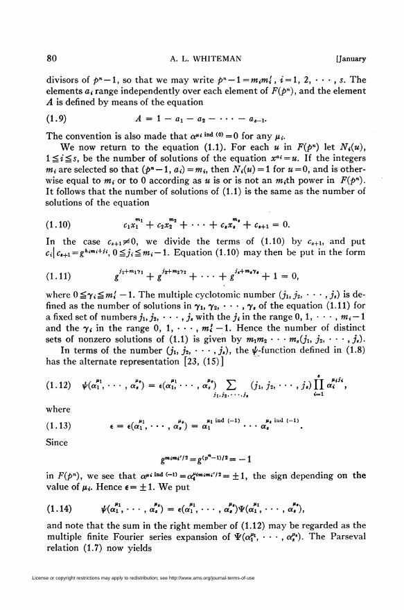
divisors of pn — 1, so that we may write pn — \ =mim'i , i = \, 2, ■ ■ ■ , s. The

elements a,- range independently over each element of Fip"), and the element

A is defined by means of the equation

(1.9) A = 1 — ai — a2 — • ■ - — a„-i.

The convention is also made that a"'ind (0) =0 for any /x,-.

We now return to the equation (1.1). For each u in Fipn) let Ni(u),

1 ¿i^s, be the number of solutions of the equation xai = u. If the integers

mi are selected so that (pn — l, ai) = mit then iV¿(«) = 1 for m =0, and is other-

wise equal to m¡ or to 0 according as u is or is not an >w¿th power in Fipn).

It follows that the number of solutions of (1.1) is the same as the number of

solutions of the equation

(1.10) ciXi + c2x22 + • • • + cex8' + c,+i = 0.

In the case cs+i9*0, we divide the terms of (1.10) by cs+i, and put

Ci\c,+i=ghimi+u, 0£ji£nti — 1. Equation (1.10) may then be put in the form

(LU) g +g +•••+« +1 = 0,

where 0^7, — wí — 1. The multiple cyclotomic number (/i,/2, • • • ,/s) is de-

fined as the number of solutions in 71, 72, ■ • • , 7« of the equation (1.11) for

a fixed set of numbersji,j2, • • • , j, with the /, in the range 0, 1, •••,».,•— 1

and the 7» in the range 0, 1, • • • , mí —1. Hence the number of distinct

sets of nonzero solutions of (1.1) is given by mim2 ■ ■ ■ ms(ji, j2, ■ ■ ■ ,js).

In terms of the number (ji, j2, ■ ■ ■ , js), the ^-function defined in (1.8)

has the alternate representation [23, (15)]

8

(1.12) 4>(d?, ■ ■ ■ , a,") = etaî,1 - - - ,a') £ 0'i- h, ' ' ' . /«) II ««' '»il.ii.---.it '=1

where

,. . ,, , fl ft. PI ind (—1) p, ind (-1)(1.13) e = e(oti , ■ • • , as ) = ai • ■ ■ as

Since

„mimi'lï = p(pn-l)/2 — —I

in F(pn), we see that a**tod (-u ■»af*»*»»'/* = +1, the sign depending on the

value of ju,. Hence e = + 1. We put

(1.14) ^(«i ,-••,«,) = «(«i , • • • , a. )Sr(ai, ■ ■ ■ , a„),

and note that the sum in the right member of (1.12) may be regarded as the

multiple finite Fourier series expansion of ^(of1, • • • , a?*). The Parseval

relation (1.7) now yields


1953] FINITE FOURIER SERIES 81

,j.)iji + ki, ■ ■ ■ ,js + ks)

Is I *(«i ■ • • . «. ) I 11 «•■Pl.Pi, ■ ■ -.P, «'"=1

We denote by F(&i, k2, ■ ■ ■ , ks) the left member of (1.15). The first part

of the present paper is concerned with the evaluation of the right member of

(1.15) (see Theorem 1). This has been carried out by Vandiver [22] in the

particular case 5 = 2. Analogous sums have been studied by Dickson [4],

Hurwitz [14], and Mordell [19]. The results have been employed to obtain

inferior and superior limits for the number of solutions of the equation (1.1)

(cf. [12]).It will be seen in several instances that our methods differ from those em-

ployed by Vandiver [22]. A major difficulty is the evaluation of the compli-

cated exponential sum p(oî\ • • • , a*") defined in (3.4) (see Theorem 2).

The remainder of the paper is taken up with the finite Fourier series ex-

pansion of the ^-function in the special case in which ai= • • • =a, (see

Theorem 3). The arithmetic sums studied by Dickson [3, (12)] and Hurwitz

[14, (30)] thus appear in a natural manner as the finite Fourier coefficients

in this expansion. In §7 we evaluate the Dickson-Hurwitz sum in the case

ßi= • • • =¡j.s^i = 0. Finally we evaluate some quadratic relations of the

Parseval type. It has been shown in another paper [25, (5.8)] that the Dick-

son-Hurwitz sums reduce to the so-called Jacobsthal sums in the particular

case w = 1, n — 1, 5 = 2. Thus Theorem 4 of the present paper may be regarded

as a far-reaching generalization of the corresponding theorem [25, Theorem 1 ]

in the theory of Jacobsthal sums.

The results of this paper may be compared with the results obtained by

Faircloth [7] and by Faircloth and Vandiver [10]. These authors discuss the

number of distinct sets of solutions of (1.1) in elements Xi, • ■ ■ , x, of Fipn).

Their methods and results for the case involving solutions in arbitrary ele-

ments are quite different from those involving solutions in nonzero elements.

The formulas are in terms of a l/'-number [10, (8)] which is equivalent to (1.8).

It may be remarked that the formulas of Faircloth and Vandiver can

be used to extend the main results of this paper to the cases in which (a)

cs+i = 0 and the x's are arbitrary elements; (b) cs+i = 0 and the x's are nonzero

elements; (c) cs+i9*0 and the x's are arbitrary elements. It turns out that the

problems involving solutions in nonzero elements are considerably more diffi-

cult than the problems involving solutions in arbitrary elements. However,

we shall not go into these questions in the present paper.

2. The \(/-iunctions. Closely related to the generalized Jacobi-Cauchy sum

(1.8) is the generalized Lagrange resolvent (cf. [23, p. 147]) defined by

(2.1) r(a") = £ a"Mrr(0),

(1.15)

llnti Z>'=i ii.it,---

(ii



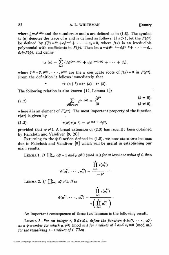
where Ç = e2rilp and the numbers a and p are defined as in (1.8). The symbol

tr (a) denotes the trace of a and is defined as follows. If «>1, let the Fipn)

be defined by fid)=6n+ci8n~1+ ■ • ■ +c„ = 0, where/(x) is an irreducible

polynomial with coefficients in Fip). Then let a = didn~1+d26n~2-\- ■ ■ ■ +d„,

diQFip), and define

n

tr (a) = Z (dit»<*-i>co + ¿20("-2>(i) + • • • + dn),i=l

where 0(1) =0, 0(2), • • • , 0(n) are the « conjugate roots of/(x)=0 in Fipn).

From the definition it follows immediately that

tr ia + b) =tr (a)+tr ib).

The following relation is also known [12, Lemma l]:

ib = 0),

ib 9* 0),(2.2) £ f***>. jf

where b is an element of Fipn). The most important property of the function

ria") is given by

(2.3) r(a")T(a-") = a" ind ^p",

provided that a"9*i. A broad extension of (2.3) has recently been obtained

by Faircloth and Vandiver [9, (9)].

Returning to the ^-function defined in (1.8), we now state two lemmas

due to Faircloth and Vandiver [9] which will be useful in establishing our

main results.

Lemma 1. If YL'-i «?' = 1 and ¡x^O imod mi) for at least one value of i, then

n *44)<*» ) =

Lemma 2. If nj=i af'^l, then

fiai , ■ ■ ■ , a, ) = -

if "' "'\fiai , - - ■ , a,) =

H r(«")

(s»r)An important consequence of these two lemmas is the following result.

Lemma 3. For an integer r, 0=r^5, define the function ^v(aîl, • • • , «?*)

as a ^/-number for which ju<^0 (mod m() for r values of i and Hi = 0 (mod mi)

for the remaining s — r values of i. Then


1953J FINITE FOURIER SERIES 83

(2.4a) .¿r-/*"" (2 = ^5,íra:, = i)!

(2.4b) Wrt = pMr~X) (íáf¿í,n¿! *Í)\

Note that r cannot equal 1 under the condition imposed in (2.4a). To

prove Lemma 3 we first note that f,(af, • • • , of*) =^r(aî1, • • • , «7"*)

is the complex conjugate of ^(«f1, • ■ ■ , of*) and that t(1) = — 1. We then

derive formulas (2.4a) and (2.4b) by applying Lemmas 1 and 2 in conjunc-

tion with (2.1) and (2.3).

We shall also make use of the function ^.(af1, • • • , a*1') whose definition

is similar to the definition of the function ^(«í1, • • ■ , of*) of Lemma 3.

From (1.13) and (1.14) it follows that |*r| 2= \xpr\2.

The case r = 0 is not covered in formulas (2.4a) and (2.4b). In this case,

however, we may establish directly the following lemma.

Lemma 4. If r = 0, then

a, ) =

P"(2.5) Mai\--- .oí")- - ((/- I)' +(-DS+1).

We have by (1.8)

(2.6) fo = ^(1, 1, • • • , 1) = X) lindernd«! . . . Jinda,-!

oí.«!,- • -.o«—1

where A is defined by (1.9). Picking out those terms in (2.6) which contain no

factor of the form l^«», we see that ^,0 = (^n_ l)»-i — NB_lt where i\7,_i de-

notes the number of solutions of the equation

(2.7) a. + a2 + ■ ■ ■ + o._i =1 (a. t*0, i - 1, 2, • • • , s - 1).

Using (2.2) together with (2.7) we get

ns_l = — X y j-f(«(«i-W""+»ri-D)P ai,a%, . . . ,a,—i-,ai^0 a

= - YJ ftr (-") YJ ftr (a^) . . . ftr (aa,-i)Í a ai,02, • • ' ,at~i\aij*0

= —(ipn - i)-i + (-i)-iir,M))

= -((#"- I)'"1 + (-!)»)•

The result stated in (2.5) now follows immediately. A proof of Lemma 4

along completely different lines is given in the thesis of Faircloth [7].



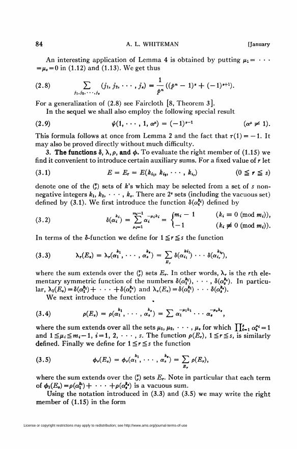
An interesting application of Lemma 4 is obtained by putting pi = • • •

=Ms = 0in (1.12) and (1.13). We get thus

(2.8) Z (/i- h ■••,/.)- ¿ ((?" - 1)' + (-l)s+1).31,32. ••■,/, ?"

For a generalization of (2.8) see Faircloth [8, Theorem 3J.

In the sequel we shall also employ the following special result

(2.9) fil,---,l,a") = i-l)^ 0*1).

This formula follows at once from Lemma 2 and the fact that t(1) = — 1. It

may also be proved directly without much difficulty.

3. The functions ô, X,p, and <f>. To evaluate the right member of (1.15) we

find it convenient to introduce certain auxiliary sums. For a fixed value of r let

(3.1) E = Er = E{kiv kh, ■ ■ ■ , kir) (Oá'ái)

denote one of the (') sets of k's which may be selected from a set of s non-

negative integers ki, k2, - - ■ , ks. There are 2s sets (including the vacuous set)

defined by (3.1). We first introduce the function 5(af0 defined by

^ -*», (nti - 1 (*, m 0 (mod «*,)),(3.2) o(c(«f ) = Is ai = \

0.-1 '— 1 (&f =zl 0 (mod mi)).

In terms of the S-function we define for 1 =r ^5 the function

(3.3) Xr(£.) = M«î*. • • • . «!') = Z «tó • ' • 5(4"),

where the sum extends over the (') sets Er. In other words, Xr is the rth ele-

mentary symmetric function of the numbers o(oi\l), • • • % °(cfy). In particu-

lar, X,(E.) =«(<#) + • • • +Ô(af) and X.(E.) =«(<#) ■ • ■ 5(o**).We next introduce the function

i*> a\ i-c\ i kl k'\ V* ~"lkl ~"'k'(3.4) p(Es) = p(ai , • • ■ , o:, ) = 2-- «i • • • a, ,

where the sum extends over all the sets pi, ¡i2, ■ • ■ , p8 for which HJ=1 of* = 1

and lá/i<á»»<— li * = !, 2, • • • , 5. The function p(Er), i^r^s, is similarly

defined. Finally we define for Igras the function

(3.5) 4>r(Es) = 4>r(a\\ ■ • • , a.') = £ p(Er),Br

where the sum extends over the (*) sets Er. Note in particular that each term

of (¡>i(Et) =p(af)+ ■ • • +p(oï*) is a vacuous sum.

Using the notation introduced in (3.3) and (3.5) we may write the right

member of (1.15) in the form



| *o(ai ,'•• ,a,)\ + X I *r(ai .•••,«.) | (Xr - *r)»••\ I2 I Y^ I .-r. / <•! '«S I2/

r=l

, P I r Í "I '*«\ I2 ,+ Is I *r(«l , • • • ■ «S ) \4

r=2

Therefore by (2.4a), (2.4b), and (2.5) we get

Theorem 1. The sum Viki, • ■ ■ , ks) defined in (1.15) is expressed by the

formula

Viki, k2, ■ ■ ■ , k.) = —- «Í- - 1)' + (-1)»+')2pin

(3.6)

+ É #»(-»Xr(£.) - Ê (>•<-« - P»<r-»)<t>riE.),r-1 r=2

w&ere Xr(£8) awd <¡>riE,) are defined in (3.3) awd (3.5) respectively.

There remains the problem of evaluating <priE,). This is accomplished

in the next section.

4. Evaluation of the p-function. Returning to the definition of the p-func-

tion in (3.4) we proceed to analyze the somewhat involved summation condi-

tion. Let m be the least common multiple of mi, m2, - - - , m,. Put w = ím,íj,

¿ = 1,2, • ■ • , s. Then we see that Uí-aO!? = 1 if and only if

(4.1) ßih + p2t2 + • • • + Pet, = 0 (mod m).

In the case where %, «21 • • • . m, are prime each to each it follows that

YLUi «í* = l if and only if p,- = 0 (mod mi), i = \, 2, • • • , s. Therefore in thiscase the sum in (3.4) is vacuous. Consequently we have proved

(4.2) PÍE,) = 0 (w, prime each to each).

Making use of (4.1) in conjunction with (3.2) we observe that (3.4) may

be written in the form

1 , , m-l

m PltPt.- ■ -.PtlPit*t> *=-0

. ! »r-K -Plki -P,k, tt-\ 2x»A(ii1f,+ -• ■+(,,«.)/»»p(E,) = — ¿^ «1 • • ' a, ¿^e

(4.3)

= -zs(«ry--a(«r')m a=o

«—» A— ku , h—k,

To evaluate the right member (4.3) we denote by 0(-Er) the number of

values of h in the range O^h^m — 1 for which A = &, (mod mi) if &<£.Er and

h^ki (mod mi) if &»(££,. In terms of the function 6(Er), (4.3) becomes

(4.4) mP(E.) = ¿ E W(».t - !)(«*, -!)•■• O«, - 1)(-1)-',


86 A. L. WHITEMAN . [January

in view of (3.1) and (3.2).

Let miEr) = [wz,,, m,-2, • ■ ■ , m,-r] be the least common multiple of a set

of r m's. In particular, m = miEs) = [mi, m2, ■ ■ ■ , m,]. For the vacuous set

Eo put w(£o) = L Related to the function 0(£r) is the function ¿(Er) which is

defined as the number of values of h in the range O^h^m — i such that

h = ki (mod mi) for each ki belonging to ET. In particular, ¿(1%) = 0(E„). For

the vacuous set E0 put /(Eo) =m. For the set £(&,-) consisting of a single k it

is clear that

tEiki) =m/mi.

To evaluate /(£■) in general we consider the system of linear congruences

(4.5) h = ¿j, (mod ?»,-,), h = &,-, (mod w,-2), ■ • • , h = kir (mod w,r),

where the numbers &,-,, Ä,-,, • • ■ , ¿,-r belong to Er and & is restricted to the

range 0 to m — \. Let d,-,-=(»»,•, m¡) denote the greatest common divisor of

mi and m¡. Then the Chinese remainder theorem (cf. [21, §5, chap. 7]) states

that the system of simultaneous congruences (4.5) is soluble if and only if

k, — kj = 0 (mod da) for every pair ki, k¡ in ET. Any solution h of this system

satisfies the congruence h = hQ (mod w(Er)), where ho is uniquely determined

(mod miEr)). Thus for 2grgiwe get the formula

Im/miEr) iki - kj = 0 (mod ¿fj); ¿,-, k¡ 6 Er),(4.6) /(£r) - \ .

lo (otherwise).

In order to express the function 0(Er) in terms of the function /(Er) we

employ a standard combinatorial argument. Let Er+q, l^q^s — r, be one

of the (j_r) sets which may be obtained by adjoining q additional k's to ET.

In accordance with this definition £r is a subset of Er+3. The problem of

evaluating 0(£r) is that of excluding from the h's counted in ¿(Er) those h's

for which h=ki (mod mi) if ki^Er. According to a general combinatorial

principle (cf. [21, theorem on p. 105]) the number of h's counted in 0(£r) is

given by the formula

BiEr) = HEr) - Z KEr+i) + Z tiEr+2) - + ■■■IA T \ Er+1 ■Br+2( • } +(-D"£<(£.)

E.

where the sum involving the sets Er+q contains ia~r) terms. In particular,

(4.7b) 0(£o) = m - Z tiEi) + £ /(£2) - E /(£8) + ••• + (-1)«/(£«).J?l E% E$

To complete the evaluation of piE,) we substitute the right member of

(4.7a) into (4.4). Our task is to pick out the coefficient of ( —l)»-r/(£r). It is

not difficult to find that this coefficient is



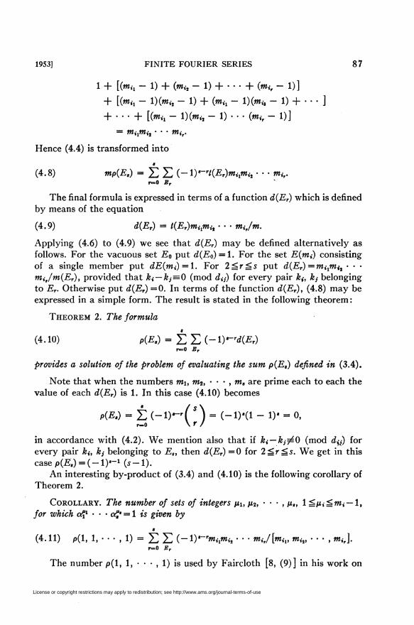
1 + [(«,, - 1) + («^ - 1) + • • • + imt, - 1)]

+ [(»,. - l)(m,-2 - 1) + (»K, - l)(w,-3 - 1) + • • • ]

+ ••• + [(»..- i)(™,2 - l)--- («<,- 1)]

= W,-,W,-2 • • • OT,r.

Hence (4.4) is transformed into

9

(4.8) mpiE,) = SI (-l)*-r/(Er)w,Iw,-2 • • • mir.r=0 Er

The final formula is expressed in terms of a function d(Er) which is defined

by means of the equation

(4.9) diET) = tiEr)mhmi, • • ■ mir/m.

Applying (4.6) to (4.9) we see that d(E,) may be defined alternatively as

follows. For the vacuous set E0 put d(E0) = l. For the set E(wz.) consisting

of a single member put ¿E(w,-)=1. For 2^r^5 put d(Er) =?w,-1w2,2 • • •

miJmiEr), provided that k{ — kj=0 (mod dtJ) for every pair £,-, k, belonging

to Er. Otherwise put d(Er) =0. In terms of the function d(Er), (4.8) may be

expressed in a simple form. The result is stated in the following theorem:

Theorem 2. The formula

(4.10) p(E8) = ¿Z(-l)'-rd(£r)r=0 Br

provides a solution of the problem of evaluating the sum piE,) defined in (3.4).

Note that when the numbers mi, m2, - - • , m, are prime each to each the

value of each d(Er) is 1. In this case (4.10) becomes

p(£.) = ¿(-i)-'(*) = (-i)*(i-i)' = o,

in accordance with (4.2). We mention also that if ki — kj^0 (mod d¡f) for

every pair ki, k¡ belonging to E„ then d(£r) =0 for 2gr^5. We get in this

casep(E3)=(-l)'-1 (5-I).

An interesting by-product of (3.4) and (4.10) is the following corollary of

Theorem 2.

Corollary. The number of sets of integers pi, p2, • • • , p„ 1 ¿ju,á»i¡-l,

for which of1 • ■ • o£* = 1 ¿5 given by

(4.11) p(l, 1, • • • , 1) = Z Z i-l)'-rmhmi2 ■ ■ ■ mir/[miv w,-2, • • • , w.-J.r=0 Er

The number p(l, 1, •• -, 1) is used by Faircloth [8, (9)] in his work on



the number of distinct sets of solutions of equations of the type (1.1).

Formula (4.11) is of importance in this connection.

As additional applications of formula (4.10) we deduce two special cases

of interest. First in the case 5 = 2 we note that mim2/[mi, m2] =di2 and thus

obtain the formula

(4.12)k¡ Jfc2 (di2 — 1

P(«l . «2 ) = <

(ki m k2 (mod du)),

(ki fá k2 (mod di2)).

The case 5 = 3 is more involved. We distinguish four essentially different

cases. First case: k\ — k2 = 0 (moddi2), k\ — k3 = 0 (moa di3) ,k2 —k3 = 0 (mod d23).

Second case: ¿i —¿2 = 0 (mod di2), k\ — &3 —0 (mod di3), k2 — k3^0 (mod d23).

Third case: &i —&2 = 0 (mod di2), £i —¿3^0 (mod du), k2 — k3^0 (mod d23).

Fourth case: &i —¿2^0 (mod di2), ki — k3féO (mod ¿13), k2 — k3f£0 (mod d23).

Formula (4.10) now reduces to

ft 4 1\ / *1 *2 *'\(4.13) p(ai , a2 , a3 ) =

mim2m3/m + 2

2 — öi2 — «13

2 — di2

2

ii diz — d2 (First case),

(Second case),

(Third case),

(Fourth case).

Other results of this nature may be deduced in a similar fashion.

5. Quadratic relations. Formulas (3.3), (3.5), (3.6) and (4.10) provide a

solution of the problem of evaluating V(ki, k2, - - - , kt).

The case 5 = 2 reduces to

(5.1)Viki, kt) = ip" - 2)2 + 6iall) + «(«?) + /S(«ï) 5(«22)

- ip"" - l)p(«i'> ot2),

where the values of the 6- and p-functions are given by (3.2) and (4.12).

Formula (5.1) leads immediately to the results of Vandiver [22, Theorem l]

mentioned in the introduction.

The case s = 3 reduces to

Viki, k2, k,) = ((/ - l)ip" - 2) + if + «(aî1) + 5(a22) + «(«?)

+ p*i6iaï)Bia?) + «(«î'Waî") + «(«ft«^))

(5.2) + p^iaMa^Siat')

— iP — 1)(p(«i . «2 ) + p(ai , a¡ ) + pia2 , a3 ))

2n n *i fc2 k3— (p — p )p(ai , a2 , a3 ),

where the values of the 5- and p-functions are given in (3.2), (4.12), and

(4.13).



We confine ourselves to two special cases of (5.2). First, in the case

ki = k2 = k3 = 0, we get after simplification

7(0, 0, 0) = (p" - Dl - 2(pn - l)3

+ (pn — l)2(wi — l)(w2 — l)(f»3 — 1) — ntim2mz/m

+ du + ¿i3 + ¿23 + 1)

+ ipn — 1)(2wiw2ot3 — mim2 — mim3 — m2m3 — mim2m3/m)

+ mim2m3.

Second, we get in the case &i —¿2^0 (mod di2), &i —¿3^0 (mod di3), k2 — k3

^0 (mod da),

V(klt k2, *,) - (p* - 1)* - 2(¿" - l)3,

provided that &i^0 (mod mi), k2^0 (mod m2), k3^0 (mod m3).

For arbitrary 5 the right member of (3.6) is a complicated expression.

However, a considerable simplification results when the numbers m,\, m2, ■ ■ ■,

m, are prime each to each. In this case we have, in view of (3.5) and (4.2),

(priai1, ■ ■ ■ , o£*)=0, i^r^s. Hence (3.6) becomes

(5.3) Viki, h, • • - , *,) - —- ((/>» - 1)* + (-1)'+1)2 + ¿ p'^KiE.)P*n r=l

provided mi, m2, • • • , m, are prime each to each.

There are two important particular cases of (5.3). In the first place,

suppose that ki = 0 (mod mi), i = l, 2, - - - , s. Then ô(af*')=>w, — 1 and

Xr(E.) is the rth elementary symmetric function of the numbers mi — 1,

m2 — 1, • • • , m, — 1. After transforming the right member of (5.3) we get the

following corollary of Theorem 1.

Corollary 1. If mi, m2, • • • , m, are prime each to each then

F(0, 0, • • • , 0) = —- Up» - 1)* + (-l)«+i)2pin

+—f-i + n(i+ («.-- i)r)Ypn \ <_1 /

In the second place, suppose that ki^O (mod mi), i=i, 2, ■ ■ ■ , s. Then

we have ô(a<*') = — 1 so thatXr(Es) = (—l)r(*). The sum in the right member of

(5.3) now becomes

¿ (-i)rf sV(r~i) = -^-^n- i)'+(-i)*+i).r=l \ r / pn

Thus we have proved

Corollary 2. If mi, m2, - - ■ , m, are prime each to each and ki^O (mod



mi), i=l, 2, ■ ■ ■ , 5, then

Vih, h, •.., kt) - —- dp» - i)« + (-i)'+1)2j)2n

(-1)«+ -^—L((#" -!)«+(-D'+1).

/>"

We conclude this section by remarking that it is not difficult to state

theorems which express the left member of

2F(0, 0, • • • , 0) - 2Viku k2,---, k.)

a

= n mi z (0'i. ■ ■ ■ ,j*) - o'i+h, ■ ■ ■ ,j,+k,))2»=1 31.32. •••.it

as the sum of squares (cf. [22, (17)]).

6. Dickson-Hurwitz sums. Let m be a. divisor of p" — 1 so that we may

write p" — i =mm'. In this and later sections the symbol (ji, j2, ■ ■ ■ , j,) de-

notes the number of distinct sets71, 72, • • • , 7», 0^7,^m' — 1, which satisfy

the equation gh+mn-}- • • • -\-g>'+m'» + l=0, for a fixed set of numbers

ii, jï, • • • > js, O^ji^m — 1. We shall expand the S^-function into a finite

Fourier series in the particular case in which ai=a2= • • • =a,=a = e2rilm. As

before we let pi, p2, - ■ - , p, denote a set of 5 non-negative integers, but we

now assume also that ju, = 1. We first prove

Theorem 3. If p denotes a non-negative integer, then the finite Fourier series

expansion of^ia""1, - • ■ , a""*-1, a") is given by

TO-l

(6.1) *(a"M, • • • , a""--i, a") = Z Dii; pi, ■ ■ ■ , p,-i)a"{,

where the finite Fourier coefficient Dii; pi, • ■ ■ , p,-i) is the Dickson-Hurwitz

sum defined by

Dii; pi, ■ • ■ , p,-i)

(6.2) = Z (lii - - " . f*-ii i — Mi/i — • • • — p.-ij.-i),31,32. ■ • -,3.-1

the numbers ji ranging independently from 0 to m — 1.

In the special case « = 1,5 = 2, Theorem 3 reduces to a result due to Dick-

son [5, (16)]. To prove (6.1) we use the fact that to every nonzero element a

in F(p") there is an element h such that gh = a. Thus we get from (1.8),

(1.13), and (1.14)

*~i■q,(aPPi, ■ ■ ■ , aw«-i, a") = Z <*" ind H IT «""*'.

Aj.Ag, • • • ,ht—i ¿=1



where the number H is defined by H— — 1 — ghl — gh2— • ■ • — gh'~l. Put

hi = my,-+/,-, OSjiúm — 1, 0^7¿ = w' —1. Then the number of solutions of the

congruence

ind i- I - ghi - ght - . . . - ghri) _(- ̂ -f . . . _|_ ,,,_!&,_! m i (mod w)

is the same as the number of solutions of the equation

— \ _ fft»Tl+3'l _ ... — «»Ti-l+ít-l = pmyt+(.i—Plh-Pr-lir-i)^

The definition of the multiple cyclotomic symbol implies that the number of

such solutions is precisely the Dickson-Hurwitz sum defined in (6.2). This

completes the proof of Theorem 3.

Putting p = 0 in (6.1) and applying Lemma 3, we obtain the result

m-l 1

(6.3) Z Dii; pi, ••• , m.-i) =-((/>"- l)«+(-l)'+1).¿=o pn

This formula was derived by Hurwitz [14, (38)] in the case n = 1, 5 = 2. It is

interesting to compare (2.8) with (6.3).

By (1.6) the finite Fourier coefficient in (6.1) is given by

1 m-l

(6.4) Dii; mi, • • • , p,-i) = — Z ^O""1, • • • . a""-1. «")«-*•.m „=o

By (1.7) the finite Parseval relation is given by

m-l

Z Dii; pi, • • • , p,-i)Dii + k; pi, • • • , m.-i)

(6.5) "v ' l m-l

= — Z I ̂ iot""1, • • ■ , a""-1, a") \2a-"k.m „=o

7. The case pi= • • • =p,_i = 0. In the special case of this section the

Dickson-Hurwitz sum (6.2) becomes

(7.1) D.ii) = Dii; 0, • • • , 0) = Z 0'i- • • • . i.-i. *)•31-32-- • -.3.-1

We shall evaluate the sum in (7.1) explicitly. Putting pi= • • • =ps_i = 0 in

(6.4) we obtainm-l

(7.2) mD.it) = ¥(1, 1, • • • , 1) + Z *(1, •••,!. *)<*-**■p=i

From (1.13), (1.14), and (2.9) we get ^(1, • • • , 1, a") = (-l)»-ia*ind <-" for

a" 9* 1. Since ind ( — 1 ) = (pn — 1 ) /2 = mm'/2 we infer easily that ind ( — 1 ) = 0

or m/2 (mod m) according as m' is even or odd. We distinguish two cases as

follows. First case: i = 0, m' even; i = m/2, m' odd. Second case: i9*0, m' even,

Í9*m¡2, m' odd. For 0=^' = *« — 1, we deduce



^ im — 1 (First case),(7.3) Z «" ind (_1)«_"< - 1

„=i I — 1 (Second case).

By Lemma 3 and (7.2), (7.3), we get after some simplification

D.ii) =

m'— iiPn - 1),_1 + (-1)*) + (-1),_1 (First case),

p*

m'— Hpn - l)"-1 + (-1)*) (Second case).

[pn

The special case 5 = 2 leads to the following well known formula due to

Mitchell [17, (2)]

[m! — 1 (First case),

(Second case).

^ im'

Z (i. 0 = \ ,,-=o Km'

8. The Parseval relation. The result (6.5) suggests the consideration of a

sum Lik; pu ■ ■ • , p„_i) defined by

m-l

(8.1) Lik; pi, ■ • • , p,-i) = Z DU; pi, • ■ ■ , p,-i)Dii + k; pu • ■ ■ , p,-i).

In the case n — \, 5 = 2 a sum equivalent to (8.1) had already been studied

by Lebesgue [16, p. 296] in 1854. The object of the present section is to

evaluate the right member of (8.1). By (6.5) we have

I m-l

iS.2) Lik; pu'" , M-i) = — Z I *(«m. • • • . a"**-1, <*") I2«""*-m M=o

In order to compute the right member of (8.2) we require some additional

notation. We put v=pi-\- • ■ • +ps-i+l and define integers /, and w< as

follows :

(/"i> m) = h, ■ ■ • , (fi,_i, m) = /,_i, iv, m) = t = t„(8.3)

m = mih = • • • = m,t,.

We emphasize that the m's thus defined are divisors of pn — 1, but are not

arbitrary divisors as in §1-5. Here the m's depend on the choice of the p's.

It is still true, however, that m = [mi, ■ ■ • , m,]. For m is a common multiple

of the numbers mi, • • ■ , m, and is therefore a multiple of their least common

multiple. If this least common multiple were not m itself, then the numbers

pi, • • • , p„_i, v would have a common prime factor. This is impossible.

We shall make use of the following lemma.

Lemma 5. Let p be a number in the range O^p^m — 1. If for O^r^s — 1, r

of the numbers ppu ■ ■ ■ , pp,-i, pv are divisible by m, and the remaining s — r

are not divisible by m, then



(8.4) | ^(a""1, ■ • • , a"!"-1, a") |2 = p«(«-r-D.

The case r=s is excluded from Lemma 5. We note, however, that all 5 of

the numbers ppi, • • • , pp,-i, pv are divisible by m if and only if p = 0. This

case is covered by Lemma 4. Lemma 5 is a consequence of Lemma 3. If

a""= 1, then exactly 5 — r + 1 of the exponents in the left member of (8.4) are

not divisible by m. This is the case covered by (2.4a). We get thus 1^1*

— pn(,-r-i)_ jf 0lP'îi then exactly s — r of the exponents in the left member of

(8.4) are not divisible by m. By (2.4b) we get again |^| *■»£»<«-«—O. In either

event we deduce Lemma 5.

We next establish the following modified version of Lemma 5:

Lemma 6. Let the integers mi, ■ ■ • , m, be defined as in (8.3). For O^r^s—1

let Er = Eimiv mi2, • ■ - , m^ be a set of r m's. If p is a number in the range

O^p^m — l for which p = 0 (mod mi) if mÊr and pÔ imodmi) if'w,-(££r,

then formula (8.4) holds.

Lemma 6 follows at once from the fact that ppt = 0 (mod m) if and only if

ju=0 (mod mi). To prove this put p,=p,;i,-. Then (p,-, m)=t{ if and only if

(pi, «*,•) = 1, and ppi=0 (mod m) if and only if ppi =0 (mod mi). The proof

is thus complete.

We now define for O^r^s

(8.5) eiEr) = Z «-**.p

where the sum extends over the values of p in the range O^p^m — 1 for

which p = 0 (mod mi) if »»,-££„ and pÔ (mod mi) if wi¿$Er. To illustrate

this definition we examine the particular case in which the p's and v are rela-

tively prime to m. If E0 is the vacuous set, then 0(EO) = m — 1 or — 1 according

as k is or is not divisible by m; if l^r^s— 1, then the sum is empty and

0(Er)=O; in the remaining case 0(ES) = 1. The number of values of p over

which the sum in (8.5) extends is, by the combinatorial principle employed

in §4, given by

m ,_ m ^ m m(8.6)-Z'-■+ Z-1-+(-l)«-r-,

m(Er) ¡¡r+l miEr+i) Er+2 miEr+2) w(£s)

where m(Er) denotes, as in §4, the least common multiple of the m's in £r.

It should be noted that the set £r in (8.6) is a subset of each of the sets

Er+q (cf. discussion after (4.6)). We are now in the position to apply Lemmas

4 and 6 to the right member of (8.2). We get thus

mLik; mi, • • • , p._i) = (1/p2") Up» - D' + (-1)'+1)2

+ Z Z p'f-^BiEr).r=0 Er



The function 0(£r) is, in many respects, analogous to the corresponding

function which appears in formula (4.7a). In order to evaluate 0(£r) we in-

troduce the auxiliary sum

(8.8) KEr) = Zfis 0(mod m(Er))

where the sum extends over the m/miEr) values of p in the range O^p^m — i

which are divisible by ?w(Er). By (8.6) we get for O^r^s.

(8.9) 0(Er) = tiEr) - Z KEr+i) + Z t(Er+2) - + •••+ (-l)^(-E.).Er + 1 -Br+2

Note in particular that (8.9) implies that 0(E„) =t(Es) = 1. We proceed to

evaluate t(Er). The values of p in the range O^p^m — 1 for which p

= 0 (mod m(Er)) may be put in the form

p=\m(Er), 0gX^w/m(Er)-l.

Thus (8.8) becomes

(8.10) tiEr) = Zexp ..„■),x \ m/miEr)/

where X runs over the integers in the range 0 ^X^wz/m(Er) — 1. The sum in

(8.10) equals zero unless X is divisible by m/miEr). Hence we have the result

(m/miEr) (* = 0 (mod «/«(£,)),(8.11) t(ET) = \

lo ik jé 0 (mod m/miEr)).

We remark that /(E0) =m if &=0 (mod m) and equals 0 if fe^O (mod m). It

is instructive to observe the analogy between (8.11) and (4.6).

There remains the problem of substituting the value of 0(Er) in (8.9)

into (8.7), and of picking out the coefficient of ( —l)r/(£r). For 0^r^5 —1 this

coefficient is

(8.12) Z i-Dk(r)pni,-k-1) = p^>-r-»ip» - Dr.

k=0 \ k /

The coefficient of

i-i)'tiE.)

is

(8.13) Z (-!)*( *V-(-*-" = —((#"" l)'+(-l)<+1).*=o \ k I p»

Introducing (8.12) and (8.13) into (8.7) we obtain the main result of this

section :



Theorem 4. If Lik; p., • • • , p,_i) is the sum defined in (8.1), then

mLik; mi, • • • , m«-i)

= _L ((r _ 1)t + (_ 1)8+i)2 + izHl ((r _ i). + (_ 1)s+i)(8.14) p2n pn

+ Z Z i-D%Er)P»^^ipn - D\

where /(£•) m defined by (8.11).

9. Special cases. When 5 = 2 the result given in Theorem 4 simplifies

considerably. We put pn — \=mm', pi=p, v=p + \, (p, m)=h, iv, m)=t2,

m=miti = m2t2. Then (8.14) becomes

mLik; p) = ip» - 2)2 + (/>« - 2) + /.«/(£„)

- Œimi)ipn - 1) - tEim2)ip» - 1).

Applying (8.11) with k=0 to (9.1) we get after a little manipulation

(9.2) ¿(0; m) = «'(i" -2) + pn- m'ih + t2).

The case k^O (mod ím) is more involved. The final formula may be ex-

pressed in the following form

m'ip»-2) iti\k,t2\k),

rn'ip" - 2) - m'h ih | k, t2\k),

m'ip" - 2) - m't2 ih\k, t2\ k),

{ rn'ip» - 2) - m'ih + t2) ih | k, h | k).

(9.3) Lik;p) =

In the case ¿1=1*2= 1 the results in (9.2) and (9.3) reduce to certain formulas

given by Hurwitz [14, (35), (36)] (w = l), and Vandiver [22, (20), (21)].

When 5 = 3 and k=0, we put (pi, m)=h, (p2, m)=t2, (pi+p2+l, m)=t3,

m = miti, m/[mi, m¡] =ti¡, and obtain

L(0; mi, Pt) = m'ip» - 2)Hp» - DiPn - 2) + 1) + p2»

- m'p»ih + t2 + t3) + m'ip» - Dih2 + h3 + t23).

For 5 arbitrary the formulas which correspond to (9.2), (9.3), and (9.4)

do not have a simple appearance. We confine our discussion to a formula

which corresponds to the first case of (9.3). Suppose that kj&0 (mod m/m(£r))

for each of the 2*-l sets £r, 0gr^5-l. Then (8.11) implies that Z(Er)=0,

0=r=5 —1, and (8.14) reduces in this case to

(9.5) Lik; pi,--- , m,_i) = ^- Up- - l)-1 + (-l)')((i* - 1)* + (~1)*+1).p n



To illustrate formula (9.5) we remark that it may be applied to the example

s = 3, p = 2ll,n = l, i» = 210, k = l, pi=14, p2 = 21.In general it does not seem possible to simplify the result in Theorem 4.

However, in the particular case in which the p's are relatively prime to m,

simpler formulas can be obtained. We put, in this case, ¿i= • • • = /„_i = l,

(y, m)=t = t„ m = mi= ■ ■ ■ =m,-i = m,t,. Returning to the formula i(£r) in

(8.11), we note that ¿(£r) = 1 for any set £r other than the vacuous E0 or the

set E(w„) whose single member is m,. The value of i(-En) is mii m\k and is 0

if m\k. The value of tEirn,) istiit\k and is 0 if t\k.

Consider next the right member of (8.14) when kj^O (mod m) and t = \.

We have in this case

Z Z i-DTWPnl-'-HPn - i)rr-0 Er

(9.6) * £(-!)'( *\p*<-r-»ip»-Dr

= _ p«'.-l) _|_ 2-1- ffpn _ 1). + (-l)rt-l),

P»

In general it is not difficult to modify the result in (9.6) appropriately to

derive the following corollary of Theorem 4.

Corollary 1. J/pi, • • -, ps-i are non-negative integers relatively prime to

m and if (pi+ • • ■ +ps_i + l, m)=t, then the value of the function

mL(k; pi, • ■ ■ , p»-i) defined in (8.1) is given as follows:

(m - t)pn(-°-l) + (t - l)/>n(*-2) (m\ k),

tpnu-v + if- DpMa~2) (t\k, m\k),

p^'-v (t\k).

We remark that an alternative proof of Corollary 1 may be deduced

directly from (8.5) and (8.7). Another special case of interest is contained in

the following corollary.

Corollary 2. Under the hypotheses of Corollary 1, the value of the sum

m-l

Z iDii; Mi, • • • , m«-i) - Dii + k; pi, - - - , p,-i))2 ik fa 0 (mod m))(_0

pinUp»- i)' + (-i)*+i)2 +

— iiP«-D° + i-D°+1)2-p¿n

h1nHP»- i)»+(-i)*+i)2

is given by



(9.7a) 2p»<-°-» ik m 0 (mod /)),

(9.7b) 2ip»<"-» - m'tp»<°-V) ik fé 0 (mod t)),

where m' is defined by the equation p»—\ =mm'.

In the case 5 = 2, w = l, / = 1 the result in (9.7a) reduces to a formula due

to Lebesgue [16, p. 298], rediscovered by Hurwitz [14, (37)], and later

generalized by Vandiver [22, (22)] to F(p»). It should be noted that (9.7a)

is a formula which gives representations of 2pn(,-1) as the sum of m squares.

Bibliography

1. H. Davenport, Note on linear fractional substitutions with large determinant, Ann. of

Math. (2) vol. 41 (1940) pp. 59-62.2. H. Davenport and H. Hasse, Die Nullstellen der Kongruenzzetafunktionen in gewissen

zyklischen Fällen, J. Reine Angew. Math. vol. 172 (1935) pp. 151-182.3. L. E. Dickson, Lower limit for the number of sets of solutions of xe+ye+ze = Q (mod p),

J. Reine Angew. Math. vol. 135 (1909) pp. 181-188.4. -, Congruences involving only eth powers, Acta Arithmetica vol. 1 (1935) pp. 161—

167.5. -, Cyclotomy and trinomial congruences, Trans. Amer. Math. Soc. vol. 37 (1935)

pp. 363-380.6. G. Eisenstein, Aufgaben und Lehrsätze, J. Reine Angew. Math. vol. 27 (1844) pp. 281-

284.

7. O. B. Faircloth, On the number of solutions of some general types of equations in a finite

field, Dissertation, University of Texas, May 1951, 36 pages. Published in Canadian Journal of

Mathematics vol. 4 (1952) pp. 343-351.8. -, Summary of new results concerning the solutions of equations in finite fields, Proc.

Nat. Acad. Sei. U. S. A. vol. 37 (1951) pp. 619-622.9. O. B. Faircloth and H. S. Vandiver, On multiplicative properties of a generalized Jacobi-

Cauchy cyclotomic sum, Proc. Nat. Acad. Sei. U. S. A. vol. 36 (1950) pp. 260-267. In Lemma 1

of this paper the condition 'V>^0 (mod mi) for any i" may be replaced by the condition

"tafáO (mod m,) for at least one value of i."

10. -, On certain diophantine equations in rings and fields, Proc. Nat. Acad. Sei.

U. S. A. vol. 38 (1952) pp. 52-57.11. H. Hasse, Bericht über neuere Untersuchungen und Probleme aus der Theorie der alge-

braischen Zahlkörper, Jber. Deutschen Math. Verein, vol. 35 (1926) pp. 1-55; vol. 36 (1927)

pp. 233-311; Ergänzungsband 6 (1930).

12. L. K. Hua and H. S. Vandiver, On the existence of solutions of certain equations in a

finite field, Proc. Nat. Acad. Sei. U. S. A. vol. 34 (1948) pp. 258-263.13. A. Hurwitz, Sur quelques applications géométriques des séries de Fourier, Ann. École

Norm. (3) vol. 19 (1902) pp. 357^108 ( = Mathematische Werke, vol. I, Basel, 1932, pp. 509-554). A simple introduction to the subject of finite Fourier series together with applications to

geometry are also given by I. J. Schoenberg, Amer. Math. Monthly vol. 57 (1950) pp. 380-404.

14. -, Ueber die Kongruenz ax'-\-bye-\-cz' = 0 (mod p), J. Reine Angew. Math. vol.

136 (1909) pp. 272-292 ( = Mathematische Werke, vol. II, Basel, 1933, pp. 430-445).15. E. Landau, Vorlesungen über Zahlentheorie, vol. 1, Leipzig, 1927.

16. V. A. Lebesgue, Demonstration de quelques formules d'un mémoire de M. Jacobi, J.

Math. Pures Appl. (1) vol. 19 (1854) pp. 289-300.17. H. H. Mitchell, On the generalized Jacobi-Kummer cyclotomic function, Trans. Amer.

Math. Soc. vol. 17 (1916) pp. 165-177.


98 A. L. WHITEMAN

18. -, On the congruence cxf + t =dy in a Galois field, Ann. of Math. (2) vol. 18 (1917)

pp. 120-131.19. L. J. Mordell, The number of solutions of some congruences in two variables, Math. Zeit,

vol. 37 (1933) pp. 193-209.20. H. A. Rademacher, The Fourier series and the functional equation of the absolute modular

invariant J(j), Amer. J. Math. vol. 61 (1939) pp. 237-248.21. J. V. Uspensky and M. A. Heaslett, Elementary number theory, New York and London,

1939.22. H. S. Vandiver, Quadratic relations involving the number of solutions of certain types of

equations in a finite field, Proc. Nat. Acad. Sei. U. S. A. vol. 35 (1949) pp. 681-685.23. -, On a generalization of a Jacobi exponential sum associated with cyclotomy, Proc.

Nat. Acad. Sei. U. S. A. vol. 36 (1950) pp. 144-151.24. A. Weil, Numbers of solutions of equations in finite fields, Bull. Amer. Math. Soc. vol.

55 (1949) pp. 497-508. For the connection with the results of Faircloth and Vandiver see

[10; 23].25. A. L. Whiteman, Cyclotomy and Jacobsthal sums, Amer. J. Math. vol. 74 (1952) pp.

89-99.

University of Southern California,

Los Angeles, Calif.


finite fourier series and equations in … fourier series and equations in finite fields by albert...

Documents