finite sample properties of bootstrap gmm for nonlinear conditional moment...

February 16, 2010 18:12 InterStat

Finite Sample Properties of Bootstrap GMM for Nonlinear

Conditional Moment Models

Rachida Ouyssea

aSchool of Economics, The University of New South Wales,Sydney, NSW 2052, Australia

()

We investigate the finite sample performance of block bootstrap tests for over-identification(J test) for nonlinear conditional models estimated using Generalized Methods of Moment(GMM). Overall, block bootstrap methods with fixed length blocks outperform the stationarybootstrap which uses a random block length. Randomizing the block length decreases thesensitivity of the distribution of the bootstrap J test and GMM estimators to the choice ofthe block size. This sensitivity diminishes with the degree of nonlinearity of the conditionalmoments. In addition, the accuracy of the block bootstrap approximation diminishes as thedimensionality of the joint test increases, especially in the tails of the distribution of the Jtest.

Keywords: Continuously-updated GMM, iterated GMM, non-overlapping and movingblocks bootstrap, stationary bootstrap, rejection probability, Q-Q-plot, Monte Carlo test.

JEL Subject Classification: 62F40; 62E17; 62G09; 91B84; 91B28; 91B25

1. Introduction

Perhaps the most popular technique for estimating conditional moment models isthe generalized method-of-moments (GMM). First introduced by Hansen [1] as analternative to maximum likelihood for the estimation of models described by condi-tional moments, GMM estimators have desirable asymptotic properties in severalcontexts. A leading example occurs in the consumption-based intertemporal asset-pricing model (C-CAPM) where the conditional moments are nonlinear functionsof the model parameters; Hansen and Singleton [2].

However, GMM estimators and the associated tests may have poor finite sampleproperties. The poor performance of the asymptotic approximation may be theresult of many reasons, two of which are the focus of this paper.

Firstly, the way the moment conditions are weighted defines two alternativeefficient estimators; the iterated GMM (IT-GMM) estimator of Hansen [1] in whichthe weighting matrix is iterated to convergence, and the continuously updatedGMM (CU-GMM) estimator of Hansen et al. [3] in which the weighting matrix isa function of the parameters of the model. Secondly, the number of conditioningvariables (instruments), used to construct the unconditional moments, determinesthe degree of over-identification of the model and the distribution of the asymptotictest. This paper pays particular attention to the finite sample bias and varianceof CU-GMM and IT-GMM and to the performance of the associated test of over-identifying restrictions (also known as the J test) defined by the GMM criterion

Tel.:+61 2 9385 3321; fax:+61 2 9313 6337.E-mail address: [email protected]

1


2

function.Tauchen [4] finds that while increasing the number of instruments reduces the

bias, IT-GMM estimators with the smallest number of instruments are the mostreliable. In addition to this bias/variance trade-off, the asymptotic chi-square testfor over-identifying restrictions tends to reject the model more often than the nom-inal level. Hansen et al. [3] find that while J test is more conservative when theweighting matrix is continuously updated, the CU-GMM fattens the distributionof the GMM estimator.

Alternative hypothesis tests and bias corrected estimators with better finite sam-ple properties are therefore of considerable interest in this context. One approachis to use the bootstrap as a simulation-based alternative to the asymptotic approx-imation. Studies of the finite sample properties of bootstrap GMM tests are scarceand limited to the case of linear models. See, for example, Hansen [5], Bond andWindmeijer [6], Lagunes [7] and Lahiri [8].

We study the finite sample properties of the bootstrap GMM inference for theclass of nonlinear conditional moment models. For dependent data, the distribu-tions of estimators and test statistics generally depend on the joint distribution ofthe observations; Leger et al. [9] and Lepage and Billard [10]. We consider nonpara-metric dependent bootstrap methods which use blocking rules to account for thetime series dependence in the sample observations. Using the C-CAPM as a labo-ratory for the Monte Carlo experiments, we compare the finite sample bias of theGMM estimators and the size distortion (i.e., the discrepancy between the nominaland the actual probability that a test rejects a true null hypothesis) of the J test forthree block bootstrap methods. The first is the non-overlapping blocks bootstrap(NOB) of Carlstein [11] which uses non-overlapping segments of the data to definethe blocks. The second is the moving blocks bootstrap (MBB) due to Kunsch [12]and Liu and Singh [13], where the blocks are defined using overlapping segmentsof the data. The bootstrap data are obtained by independent sampling with re-placement from among the blocks. The block length in both NOB and MBB isnonrandom and must grow with the sample size in order to achieve consistency.The third is the stationary bootstrap (SB) of Politis and Romano [14]. In the SB,the lengths of the resampled blocks are random and have a geometric probabilitydistribution. Politis and Romano [14] show that the bootstrap sample generatedby randomizing the block length is stationary. In the context of estimating the biasand the variance of smooth functions of the population mean, Lahiri [8, 15] findthat the MBB outperforms the NOB which in turns outperforms the SB.

The paper also explores the usefulness of the block bootstrap as a finite-samplesize-reduction for the J test when the model parameters are nearly under-identifiedand the instruments are weak.

The findings of the simulation study can be summarized in the following. Thebootstrap test based on any of the blocking methods outperforms the asymptoticχ2−approximation. In terms of approximating the size of the J test, the blockbootstrap with nonrandom block lengths is more accurate than the stationarybootstrap. The latter is the least sensitive to the choice of the block length. Further,the simulation evidence suggests that the nonlinearity in the moment functionsaffects the sensitivity of the bootstrap approximation to the blocking rule. Finally,the accuracy of the block bootstrap in approximating the tails of the distributionof J test decreases with the dimensionality of the joint tests.

The paper is organized as follows. Section two reviews the GMM estimationand its asymptotic properties. Section three defines the bootstrap methods. Sec-tion four describes the calibrated model and the Monte Carlo environment. Sectionfive presents the finite sample properties of the GMM estimators and the asymp-


3

totic test for over-identification. Section 6 discusses the statistical properties of thebootstrap tests.

We use the following notation throughout the paper: E (.|It) is the expectationof the argument conditional on some suitable information set It available at timet, E (Zt) is the unconditional expectation of Zt, E F (.) is the (unconditional) expec-tation under the probability distribution F , the indicator function Ind(A) takesthe value 1 if the statement “A” is correct and 0 otherwise, A−1 is the inverse ofA, ιm is a m-vector of ones, Im is an m×m identity matrix, diag(A) is the vectorconsisting of the diagonal elements of A, tr(A) is the sum of the diagonal elementsof A, the norm of A is ‖A‖ = (tr(A′A))1/2, A⊗B is the Kronecker product of A andB, i.e., for A = [aij ], A ⊗ B = [aijB], iid stands for ‘independent and identicallydistributed’ and, ‘vector’ means a column vector.

2. GMM for the class of conditional moment models

Models that are defined in terms of conditional moment restrictions establish thatcertain parametric functions have zero conditional mean when evaluated at thetrue parameter values. Let Ytnt=1 be an ergodic and stationary time series vectorof endogenous and exogenous random variables. The coordinates of Yt are relatedby an econometric model that establishes that the true distribution of the datasatisfies the conditional moment restrictions

E [h(Yt+1, θ0)|It] = 0, t = 1, ..., n− 1, (2.1)

for a unique value of the k-vector θ0 ∈ Θ, where Θ ⊂ Rk and h(Yt+1, θ0) is an

m−dimensional parametric function. The function h can be understood as theerrors measuring the deviation from an equilibrium condition.

Suppose that we can form an n × q matrix Z with typical row zt such thatall its elements belong to It. The q variables given by the columns of Z are calledinstrumental variables, or simply instruments. These instruments are required to be‘predetermined’ and not necessarily ‘econometrically’ exogenous. That is, currentand lagged values of Y are valid instruments.

Given the conditional moment restriction (2.1) and the additional assumptionthat the constituents of h(Yt+1, θ0) and the variables in zt have finite second mo-ments (Hansen and Singleton [2]), a family of (unconditional) population orthog-onality conditions

E [g(Xt, θ0)] = 0, (2.2)

can be constructed where Xt ≡ (Yt+1, zt), g(Xt, θ0) = h(Yt+1, θ0)⊗zt and providedthat q ×m (henceforth mq) is at least as large as k. The moment restrictions in(2.2) are also known as the estimating equations.

The generalized methods-of-moments estimation uses the sample versions of thepopulation orthogonality conditions (2.2) to construct an estimator for θ0. TheGMM estimator θ is

θ = arg minθ∈Θ

gn(X , θ)′Wngn(X , θ), (2.3)

gn(X , θ) =1n

n∑

t=1

g(Xt, θ), (2.4)


4

where Wn is a sequence of symmetric positive-definite weighting matrices whichconverge to a positive definite matrix W when n goes to infinity, Θ is a compactparameter space, Θ ⊂ R

k, and X = X1, ..., Xn. Regularity conditions for theconsistency of the GMM estimator θ in (2.3) include: (a) gn(X , θ) converges toE (g(Xt, θ)) uniformly in θ ∈ Θ, (b) E (g(Xt, θ)) 6= 0 for all θ 6= θ0, (c) E (g(Xt, θ))and gn(X , θ) are continuously differentiable and, ∂gn(X ,θ)

∂θ converges to ∂E (g(Xt,θ))∂θ . If

in addition, (d)√ngn(Y, θ0) converges in distribution to a normal distribution with

mean zero and variance Vg > 0 and, (e) the mq × k matrix G0 = ∂E (g(Xt,θ))∂θ′ |θ=θ0

has full rank k, then√n(θ− θ0) converges in distribution to a normal distribution

with mean zero and asymptotic variance

AsyV (θ) =(G′0WG0

)−1G′0WΩ0WG0

(G′0WG0

)−1, (2.5)

Ω0 = E[g(Xt, θ0)g(Xt, θ0)′

]. (2.6)

See Davidson and MacKinnon [16] and Greene [17] for a discussion of the asymp-totic properties of minimum distance estimators.

Assumption (b) is the global identification which requires that the populationmoment condition only holds at one parameter value in the entire parameter spaceΘ. In nonlinear models, it is rarely possible to derive testable conditions for globalidentification. This assumption is replaced by assumption (e), which is a localidentification condition defined in a neighborhood of θ0. It is also known as thefirst order identification condition, see Dovonon and Renault [18].

The covariance matrix of g(Xt, θ0) has the form in (2.6) because the momentfunctions h(Yt+1, θ)⊗ zt∞t=1 are martingale first differences. This is a direct im-plication of the conditional moment restriction (2.1). With the asset pricing ap-plication in mind, this moment condition is consistent with an economy whereinvestors hold assets for one period. The moment condition can be made moregeneral by considering an economy where assets are held to maturity s > 1

E [h(Yt+s, θ0)|It] = 0, t = 1, ..., n. (2.7)

The assumption of s > 1 does not affect the asymptotic properties of the GMMestimators. However in finite samples, the difficulty in accurately estimating thespectral density matrix (long run variance) of the moment functions is an additionalsource of poor finite sample performance of the asymptotic approximation. See, forexample, Burnside and Eichenbaum [19].

The optimal weight matrix W0 which minimizes (2.5) is W0 = Ω−10 . The covari-

ance matrix of the efficient GMM estimator is AsyV (θ) =(G′0Ω−1

0 G0

)−1 and isoptimal in the class of GMM estimators with this set of moment conditions.

2.1. The iterative GMM estimator

In practice, the efficient GMM estimator is unfeasible since Ω−10 is not known.

Hansen [1] shows that a consistent estimator of Ω0 is sufficient for asymptoticefficiency. If θ is a consistent estimator for θ0, then

Ωn(θ) =1n

n∑

t=1

g(Xt, θ)g(Xt, θ)′, (2.8)

is a consistent estimator for Ω0.


5

An efficient two-step GMM estimator, denoted θ(2), is based on a weight matrix

Wn(θ(1)) = Ωn

(θ(1))−1

,

where θ(1) is a consistent one-step estimator for θ0 based on a weighting matrixequal to the identity matrix.

The iterative GMM estimator IT-GMM, denoted θit, continues from the two-step estimator by reestimating the weighting matrix. For each subsequent stepl = 3, .., L, the weighting matrix is updated using Wn(θ(l−1)) = Ωn(θ(l−1))−1,where θ(l−1) is the consistent estimator when Wn = Wn(θ(l−2)) . This is repeateduntil l attains some large value L, we choose L = 15, or until convergence definedas ‖Wn(θ(l+1))−Wn(θ(l))‖ < 1E − 4.

2.2. The continuous updating GMM estimator

Instead of taking the weighting matrix as given in each iteration, Hansen et al.[3] propose an estimator in which the weighting matrix is continuously updated.Formally, the CU-GMM estimator, denoted θcu, is

θcu = arg minθgn(X , θ)′Ωn(θ)−1gn(X , θ), (2.9)

where Ωn(θ) = 1n

∑nt=1 g(Xt, θ)g(Xt, θ)′.

2.3. Wald test for over-identifying restrictions

The first order conditions for minimizing (2.3) is a system of k equations with kunknowns

∂gn(X , θ)′∂θ

Wngn(X , θ) = 0.

There are mq − k remaining linearly independent moment conditions that are notset to zero in the estimation. These must be close to zero if the model is correct. Inan over-identified model, mq > k and there may not be a parameter value θ thatsatisfies (2.2). The model and the moment restrictions are therefore testable. Thestandard test statistic for over-identifying restrictions (also called J test) is basedon the minimized GMM criterion function,

Jn(θ) = ngn(X , θ)′Ωn(θ)−1gn(X , θ). (2.10)

When the moment conditions are valid, the J test has an asymptotic chi-squareddistribution with mq − k degrees of freedom. See Hansen [1] for an exposition ofthe general theory of GMM estimation and testing. It is worth noting that theJ test statistic is a Wald test for the hypothesis, E (g(Xt, θ0)) = 0. The latteris a joint hypothesis with mq individual moment restrictions. In finite samples,the number of unconditional moments mq affects the accuracy of the chi-squaredapproximation. The finite sample size (i.e., rejection of a true null) of the J testincreases uniformly as the dimension of joint tests increases and is drastically largerthan the asymptotic size of the test. See Burnside and Eichenbaum [19].

Economic theory often provides information about m, the number of conditionalmoment restrictions. For example, the Euler equation of a decision theoretic prob-


6

lem. However, the number of instruments q is often arbitrarily determined by thepractitioner. This paper investigates whether the bootstrap can provide improvedfinite sample inference in over-identified models.

3. Bootstrap GMM

3.1. Preliminary

Let X1, X2, · · · be a sequence of stationary random variables with unknown jointprobability distribution F0 indexed by an unknown real-valued parameter θ0. Con-sider a statistic of interest, Tn(θ0), which is possibly a function of F0 through θ0,

Tn(θ0) = Tn(X , F0), (3.1)

where X = Xt, t = 1, · · ·, n is the original sample. The bootstrap uses anonparametric estimate Fn of F0 to approximate the distribution of Tn usingT ∗n = Tn(X , Fn). To obtain asymptotic refinements, bootstrap sampling must takeinto account the dependence of Xt in the population data generating process.

In an attempt to reproduce different aspects of the dependence structure of theobserved data in the bootstrap sample, different block bootstrap methods havebeen proposed in the literature. We briefly describe three of these methods.

Non-overlapping blocks bootstrap, NOB

The base sample, X , is divided into φ blocks of pre-specified length ω such thatφω = n. Denote these blocks by Bi, i = 1, 2, · · ·, φ where B1 = Xt, t = 1, · · ·, ω,B2 = Xt, t = ω + 1, · · ·, 2ω, Bs = Xt, t = ω(s − 1) + 1, · · ·, ωs, and so forth.The NOB is implemented by randomly sampling with replacement φ blocks fromBi, i = 1, 2, · · ·, φ. The selected blocks are laid end to end to form the bootstrapsample X ∗.Moving blocks bootstrap, MBB

We use the following overlapping block bootstrap procedure, which is originallyattributed to Kunsch [12]. Let I = 1, 2, ···, n−ω+1 denote the set of observationsthat can begin a block of ω observations. The construction of the bootstrap sample,Bi, i = 1, · · ·, φ, begins by random sampling from I with replacement φ times.Let Qi, i = 1, ..., φ be the random sample from I. The MBB sample consistsof the φ blocks which begin with the observations Qi, i = 1, · · ·, φ. The firstblock in the bootstrap sample is B1 = XQ1+i, i = 1, · · ·, ω, the jth block isBj = XQj+i, i = 1, · · ·, ω for j = 1, · · ·, φ. These blocks put together form thebootstrap sample, X ∗ = Bj , j = 1, · · ·, φ.Stationary bootstrap, SB

Unlike the NOB and MBB, the stationary bootstrap of Politis and Romano [14]uses a random block length to generate the bootstrap sample. Let L1, L2, · · · be asequence of iid random variables having a geometric distribution with parameterp = ω−1 ∈ (0, 1). That is, for m = 1, 2, · · ·, the probability of an event, Li = m,is (1− p)m−1p.Independent of Xi and Li, let I1, I2, · · · be a sequence of iid variables that havea discrete uniform distribution on 1, · · ·, n. The first block B1 consists of L1

observations, B1 = XI1 , · · ·, XI1+L1−1. The next sampled block B2 consists ofL2 observations, B2 = XI2 , · · ·, XI2+L2−1, and so forth. In other words, the firstobservation X∗1 is sampled randomly from X ; X∗1 = XI1 . For j = 2, · · ·, n, if the


7

(j − 1)th observation in the bootstrap sample is X∗j−1 = Xk, then

X∗j =Xk+1 with probability pXIj with probability 1− p

Blocking rule

Hall et al. [20] show that the asymptotically optimal blocking rule is ω ∼ nκ

where κ minimizes the mean-square error (MSE) of the block bootstrap estimator.They find that κ = 1

5 is optimal for estimating a double sided distribution, suchas the t − statistic, and κ = 1

4 is optimal for estimating a one-sided distribution,such as the J test for over-identification.

The three bootstrap methods have different asymptotic properties in terms ofefficiency and MSE. Politis and White [21] show that the asymptotic relative ef-ficiency of MBB relative to SB is always bounded away from zero. They arguethat although the MBB is asymptotically more efficient, it is more sensitive to thechoice of block size. Using expansions of the bias, the variance and the MSE, Lahiri[15] finds that MBB is to be preferred to NOB and that the random block lengthleads to MSE larger than those for nonrandom block length.

In this paper, a grid of values of p and ω are used to compare the three bootstrapmethods in terms of the mean and median bias, and the size of the J test. To linkthe fixed block length ω of the NOB and the MBB to the random block length ofthe stationary bootstrap, we choose ω equal to the expected block size of the SB;ω = E(Lk) and p = 1/ω = φ/n.

3.2. Bootstrap test for over-identification

Bootstrapping GMM is not standard; in over-identified models the population mo-ment conditions (2.1) do not hold exactly in the bootstrap sample. The bootstrapsample X ∗ does not satisfy the same moment conditions as the population distri-bution. The recentering proposed by Hall and Horowitz [22] replaces the bootstrapmoment functions, g(X∗t , θ), with

g∗(X∗t , θ) = g(X∗t , θ)− gn(X , θ), t = 1, · · ·, n. (3.2)

This recentering makes the J test asymptotically pivotal and preserves the higherorder refinements of the bootstrap. In this paper, we adopt this recentering of themoment functions to compute the bootstrap IT-GMM and CU-GMM estimatorsand the three bootstrap tests for over-identification.

Let g∗n(X ∗, θ) = 1n

∑nt=1 g

∗(X∗t , θ), the bootstrap GMM estimator, θ∗, solves

θ∗ = arg minθ∈Θ

g∗n(X ∗, θ)′W ∗ng∗n(X ∗, θ). (3.3)

The bootstrap CU-GMM estimator, θ∗cu, solves (3.3) for W ∗n = Ω∗n(θ)−1, where

Ω∗n(θ) =1n

n∑

t=1

g∗(X∗t , θ)g∗(X∗t , θ)

′. (3.4)

The bootstrap IT-GMM estimator, θ∗it, solves (3.3) for W ∗n = Ω∗n(θl−1)−1, whereθ(l−1) is a consistent estimator that solves (3.3) for Wn = Ω∗n(θ(l−2))−1. This is


8

iterated until convergence is achieved or a maximum number of iterations, L = 15,is reached.

Hall and Horowitz [22] propose new formulae to correct the J test for the differ-ences between the asymptotic covariances of the original sample and the bootstrapvariances. These corrections preserve the higher order expansions that produce thehigher order refinements. Andrews [23] generalizes the correction factors to thecase of MBB bootstrap. The distribution of the J test statistic is approximatedusing the following statistic,

J∗n(θ) = ng∗n(X ∗, θ)′W ∗12

n V +n W

∗ 12

n g∗n(X ∗, θ),

where V +n denotes the Moore-Penrose generalized inverse of the correction matrix

Vn,

Vn = MnW12n WnW

12n Mn, (3.5)

Mn = I − Ω− 1

2n Gn[G′nΩ−1

n Gn]−1G′nΩ− 1

2n , (3.6)

where Ωn = Ωn(θ), Gn = ∂gn(X ,θ)∂θ |

θ=θ, θ is the GMM estimator calculated using

the original sample X , and

Wn =1n

φ−1∑

i=0

ω∑

j=1

ω∑

s=1

g∗(Xiω+j , θ)g∗(Xiω+s, θ)′ (3.7)

for the non-overlapping blocks, and

Wn = φn−1(n− ω + 1)−1n−ω∑

i=0

ω∑

j=1

ω∑

s=1

g∗(Xi+j , θ)g∗(Xi+s, θ)′ (3.8)

for the overlapping blocks.For the stationary bootstrap, Vn = Imq. In the case of martingale first difference

moment functions, Wn = Ω∗n(θ) in (3.7) and the correction factor is equal to theidentity matrix, Vn = Imq. See the proof in Appendix 1.

4. The Monte Carlo environment

4.1. The calibrated model

Consider a representative consumer with intertemporally separable constant riskaversion preferences, and an economy with m assets traded in complete and fric-tionless markets. The Euler equation in the consumption capital asset pricing modelis as given in equation (2.1) with

h(Yt+1, θ) = β(ct+1)−γ ⊗Rt+1 − ιm, (4.1)

where Yt = (ct, R′t), θ = (γ, β)′, ct is the growth rate of consumption, Rt is the mdimensional vector of gross stock returns, γ is the risk aversion parameter (> 0),β is the impatience parameter, and ιm is an m× 1 vector of ones. The one period


9

gross return from holding one unit of stock j is defined as:

Rj,t+1 =Pj,t+1 +Dj,t+1

Pj,t, j = 1, · · ·,m,

where Dj,t+1 is the dividend yield on stock j from period t to t+ 1.We follow Kocherlakota [24] and consider three assets; m = 3. The Risk free Rf

which pays one unit of consumption, the market portfolio MP which pays Ct unitsof consumption in period t, and the stock market SM with dividend payoffs Dt inperiod t.

To simulate series of consumption growth and stock returns that satisfy themoment conditions (2.1) and (4.1), we use the quadrature approximation originallyintroduced by Tauchen and Hussey [25]. See also Tauchen [4, 26], Kocherlakota [24]and Wright [27].

Let y t = (log(ct), log(dt))′, where dt = Dt/Dt−1 is the dividend growth, be a

vector of jointly stationary first order Markov processes. The quadrature approx-imation fits an N state Markov chain to yt so as to approximate the first ordervector autoregression (VAR)

y t = µ+ Φy t−1 + εt, (4.2)

where εt are iid with E (εt) = 0 and V (εt) = Vε, µ = E (y t) and Φ = Φij, i, j =1, 2, is the VAR matrix of coefficients. For computational considerations, we chooseN = 8. Tauchen and Hussey [25] find that an 8−point rule generally yields accuracyclose to four digits in terms of mean-squared error. Appendix 2 provides a detaileddescription of the quadrature procedure, and a description of how the series ofassets returns Rf , MP and SM are generated using the conditional moments(4.1), and the series ct and dt.

[Table 1 about here.]

4.2. Parameter and preference setting

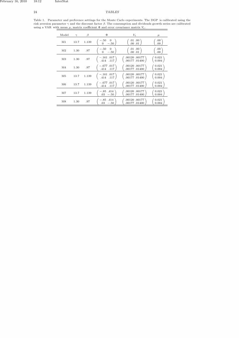
Table 1 lists the combinations of the parameters γ, β, Φ, Vε, and µ for the modelswe consider in the Monte Carlo simulations. We are particularly interested in threecharacteristics of the data generating process of yt. First, the serial correlation inthe consumption series, Φ11, and in the dividends growth series, Φ22. Second, theinteraction between log(ct) and log(dt) in the VAR determined by the parametersΦ12 and Φ21. This is also known as the Granger-Sims effect allowing for feed-back from log(dt−1) to log(ct) through Φ12, and from log(ct−1) to log(dt) throughΦ21. Third, the degree of nonlinearity in the moment function measured by themagnitude of the coefficient of relative risk aversion γ.

We consider two sets of values for θ. The first is θ1 = (1.30 0.97 )′, used inTauchen [4], and the second is θ2 = (13.7 1.139 )′ from Kocherlakota [24].

The first two models, M1 and M2, are used as benchmarks where the con-ventional asymptotic theory is expected to work well. M2 is the full rank modeldescribed in Wright [27]. It satisfies the first order identification assumption of fullrank matrix G0. Models M3 and M5, represent VAR specification as estimated byKocherlakota [24] when the VAR is fitted to U.S. annual data. These are weaklyidentified models where the matrix G0 has rank 2 but is close to being rank de-ficient, see Wright [27]. Models M4, M6 and M7 are introduced for comparativepurposes as cases of unrealistically strong serial correlation while maintaining theGranger-Sims feedback between the VAR series.


10

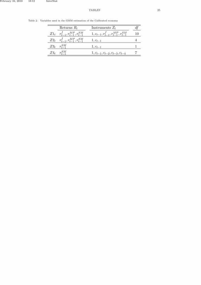
To study the effect of the degree of over-identification mq − k, we consider in-struments with small and large number of variables. In addition to a column ofones, the case of Zt = Z2t consists of the series of lagged consumption growthct−1 and the case of Zt = Z1t consists of 4 variables, ct−1 and lagged returnsRt−1 = (rft−1, r

MPt−1 , r

SMt−1 )′. In practice the market portfolio is not observable, there-

fore we omit rMPt−1 in Z3t. The case of Z4t represents a situation where the number

of instruments is increased by taking additional lags of the same variable. Weconsider two sample sizes n = 120 and n = 500.


4.3. Monte Carlo algorithm

This paper compares the rejection probability of the asymptotic and block boot-strap J test under the null data generating process (DGP). Let µ0 denote the trueDGP, µ∗ the bootstrap DGP generated by Fn, and τ an asymptotically pivotaltest statistic. The rejection probability of the bootstrap test at nominal level αunder µ0 is RP = Pµ0(τ < Q(α, µ∗)), where Q(α, µ∗) is the α quantile of τ underµ∗. Using M Monte Carlo replications, an estimate RP of this probability can beobtained,

RP =1M

M∑

s=1

Ind(τs ≥ Q∗(α, µ∗)), (4.3)

where Q∗(α, µ∗) is the α quantile of τ∗, the bootstrap statistic, under µ∗. For eachreplication, the quantity (4.3) requires the calculation of B bootstrap samples.This implies, M(B + 1) test statistic calculated for each Monte Carlo experiment.This turns out to be computationally prohibitive because of the nonlinearity of themoment conditions and the computational demand of the CU-GMM algorithm.Davidson and MacKinnon [28, 29] propose very fast methods to obtain approxi-mations to RP with the computational effort of only 2M + 1 visits to (2.3) and(3.3). See, for example, Lamarche [30], Richard [31], and Ahlgren and Antell [32]for discussions of the performance of fast bootstrap inference and applications.

For a given DGP in Table 1 and a given value of the random block probability p,the (fast bootstrap) algorithm below is implemented for the NOB, the MBB andthe SB bootstrap under both the iterated and the continuously updated GMM.We consider 18 values of p; p ∈ 0.05, 0.10, · · ·, 1 and ω = 1/p. We describe thefast bootstrap algorithm as follows.

[Figure 1 about here.]

Step 1 For s = 1, ...,M , where M = 10, 000,a) We generate a random sample of size n of consumption and dividends

growth. We use the quadrature approximation to generate returnsseries that satisfy (2.1) and use the sample data, X , to compute theGMM estimates θ(s) and the J test value J (s).

b) We generate one single bootstrap sample X ∗ and compute the boot-strap GMM estimates θ∗(s) and the bootstrap J test , J∗(s).

Step 2 At the end of Step 1, we have a sequence of sample statistics θ(s), J (s),and bootstrap statistics θ∗(s), J∗(s) for s = 1, · · ·,M .Let Q∗(α) be the α quantile of the bootstrap J test, J∗. Using the ap-proximation proposed by Davidson and MacKinnon [29], we estimate the


11

rejection probability, RP , and the error in rejection probability, ERP ,

RPA ≡1M

M∑

s=1

Ind(J (s) ≥ Q∗(α)

), (4.4)

ERP ≡ RPA − α. (4.5)

5. Finite sample properties of GMM estimators and J test

5.1. Statistical properties of J

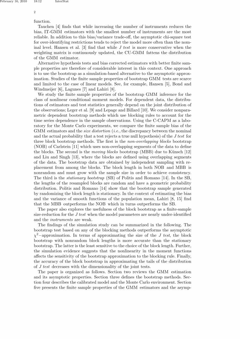
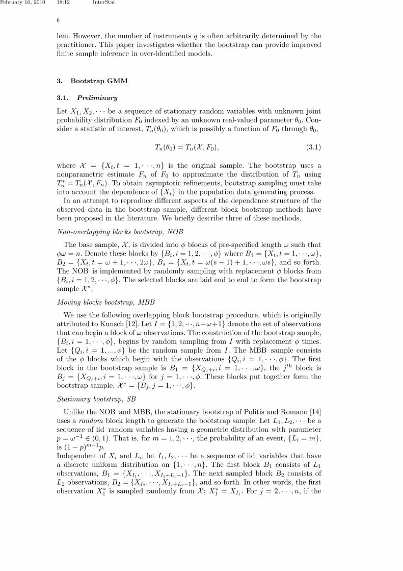
Figure 1 is a plot of the kernel density estimates for J along with the density of theasymptotic chi-squared test (χ2

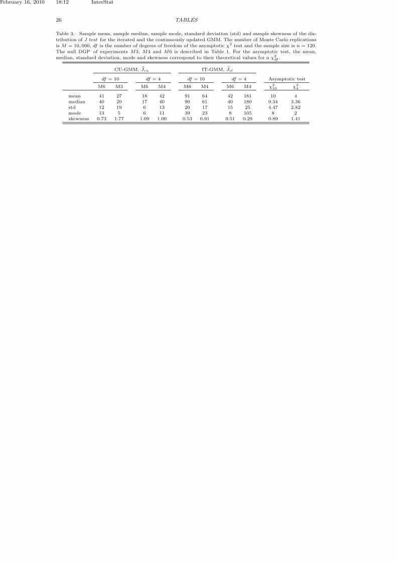
df , df = mq − k). Table 3 reports sample summarystatistics for central location (mean, median and mode), standard deviation andsample skewness for J under a selection of DGPs from Table 1.


The results support the existing evidence that the asymptotic approximationperforms very poorly in finite samples. In Table 3, regardless of the weightingmatrix used to construct the GMM criterion in (2.3), the sample mean, median andmode of J are significantly higher than those of the χ2 distribution. In addition, thedistribution of J is more dispersed and generally less skewed than the asymptoticapproximation. The kernel density estimates in Figure 1 provide further evidencefor the departure of the finite sample distribution of J test from its asymptoticapproximation. The asymptotic χ2 test suffers severe size distortion leading tospurious rejection of the C-CAPM model.

A number of interesting distributional patterns emerges from our study of theeffect of the DGP properties on the distribution of the J test. We find that at leastfour factors impact the quality of the asymptotic approximation.

First, consider Figure 1a where the distribution of CU-GMM test, Jcu, is gen-erated using the DGP in experiments M1 and M6. In these experiments, thetransmission of the dynamics between the variables in the VAR is enabled bynon-zero VAR parameters Φ12 and Φ21.

In the remainder of the paper, we use the terms Granger-Sims and transmissionchannels to indicate this interaction between lct and dt through their lagged values.In the DGP of model M1, there is no correlation between log consumption andlog dividends growth while in M6 there is positive feedback from log(ct) to log(dt)(Φ21 = 0.414). The distribution of Jcu moves further away from the χ2 as moreinteraction is introduced between the VAR variables. This result is similar to thatof Tauchen [4] who finds that introducing positive feedback from consumption todividend growth tends to raise the bias of the iterated GMM estimator.

Second, to illustrate the effect of the degree of nonlinearity, γ, in the momentfunction (4.1), Figure 1b plots the kernel density estimates of Jcu under DGPM3 (small γ0 = 1.30) and DGP M5 (large γ = 13.7). Our findings suggest thatincreased nonlinearity causes the distribution of J to shift further away from theχ2 approximation. This is consistent with Tauchen [4] finding that larger values ofγ tend to move the bias in the IT-GMM of γ downward.


Third, the weighting matrix Wn in (2.3) impacts the distribution of the over-identification test. Figure 1c plots the kernel density estimates for the IT-GMM


12

statistic, Jit, and the CU-GMM statistic, Jcu, and Table 3 reports their summarystatistics. The iterated GMM test, Jit, has significantly larger mean, median andstandard deviation than Jcu. The distribution of the continuously updated GMMis however more skewed with heavy tails.

Finally, Figure 1d shows that increasing the serial correlation in the log of con-sumption growth series (from −.161 in M3 to −.677 in M4) shifts the body of thekernel density estimate of J to the right with higher median and more skewness. InFigure 1a-1d, as the body of the kernel density shifts towards the right, the densitycurve becomes more centered and less skewed.

5.2. Statistical properties of the GMM estimators

Our analysis hereafter focuses on the continuously updated GMM estimator. Evi-dence from Monte Carlo simulations (not reported here but available upon request)suggests that the main conclusions are qualitatively valid for both the CU-GMMand IT-GMM estimators.

Table 4 presents the summary statistics for the distribution of θcu for an economycalibrated with preference parameters γ0 = 13.7 and β0 = 1.139. Panel A highlightsthe feedback effect discussed earlier. The GMM estimator under the DGP of modelM2 has the least mean and median bias for γ. Although the serial correlation inM5 is weaker, the specification introduces strong feedback from lct to dt. Theestimates are biased upward suggesting similar conclusions to those of Tauchen [4]who argues that “positive association between dividend and consumption growthtends to counteract the downward bias and may produce upward bias.”

Panel B highlights the effect of an increase in the sample size from 120 to 500.While the mean and median bias decrease marginally with the number of obser-vations, there is a significant drop in the standard errors and the overall meansquared error of the estimates of the model parameters.


It is worth noting that in addition to its poor approximation in finite samples,the asymptotic theory developed in Hansen [1] is unreliable in large samples underweak identification or weak instruments, which may be manifested in the MonteCarlo experiments.

First, models M3 and M5 in Table 1 are nearly rank deficient (Wright [27]). Ina model with nonlinear moment conditions, global identification (assumption (b))can hold without the rank condition (assumption (e)) being satisfied. Dovonon andRenault [18] derive the asymptotic properties of the J test when the parametervalue is globally identified but the matrix G0 is rank deficient. They find thatthe J test is asymptotically distributed as half and half mixture of χmq−k andχmq−k−1. Hansen [1]’s asymptotic χ2

mq−k assumes first order identification andleads to significant over-rejection rate.

Earlier, we noted the small improvement in the bias and standard errors whenthe sample size increases. This may be attributed to the slow rate of consistency,OP (n−1/4) instead of OP (n−1/2), reported by Dovonon and Renault [18].

Second, the instruments used to construct the unconditional moments (2.2), maybe weak. This means the moment restriction E [g(Xt, θ)] is uniformly close to zeroover the parameter space and does not permit to identify θ. In their analysis ofinstruments’ weakness, Antoine and Renault [33] note that the moment restrictionsvary quite substantially with the constant term as instrument while remains fairlysmall when Zt consisted of lagged consumption growth and asset returns.


13

6. Block bootstrap finite sample inference

The simulation evidence suggests that the estimates of the bootstrap rejectionprobability RPA depend on the number of over-identifying restrictions (degrees offreedom), the VAR structure (serial correlation and Granger-Sims feedback), andthe degree of nonlinearity of the moment functions (parameter γ). This is also truefor the sample mean, median, mode, standard deviation and skewness of the kerneldensity estimate of the distribution of J∗.


6.1. Bootstrap GMM inference and the number of instruments

Table 5 reports the sample measures of location, dispersion and skewness for theblock bootstrap J∗. Consider first the case where the null DGP is calibrated usingγ0 = 1.30. Panel A reports sample summary statistics when Z1 is used to con-struct the unconditional moment restrictions (2.2). The number of over-identifyingrestrictions in this case is df = 10. Panel C presents the results for the case ofZ = Z2 with smaller number of instruments and df = 4. Additional momentrestrictions that result from increasing the number of instruments improves thebootstrap approximation for the mean, the median and the mode of the distribu-tion of J . However, increasing the number of instruments almost always results inhigher standard errors.


In panels B and D of Table 5, the moment functions are highly nonlinear as in thecase of γ0 = 13.7. Additional moment restrictions in the form of additional instru-ments worsens the bootstrap approximation. In fact, the bootstrap approximationperforms better when Z = Z2. In this case, the measures of central location for J∗

are the closest to those of J .


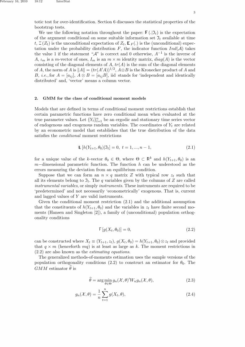
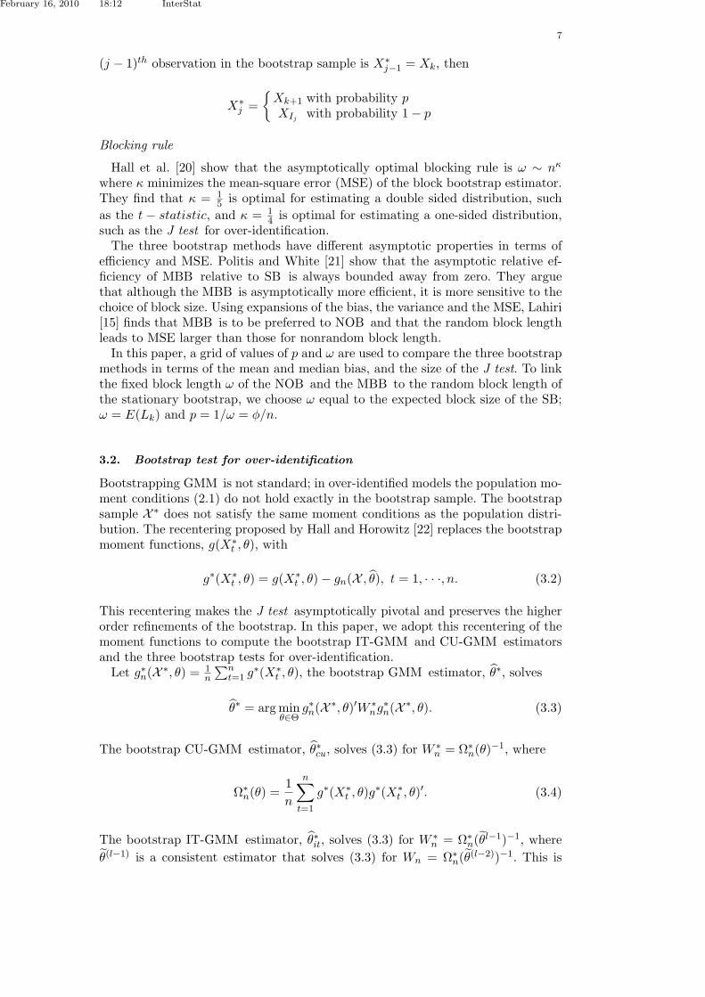
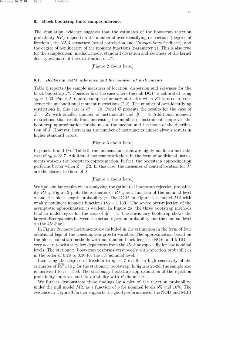
We find similar results when analyzing the estimated bootstrap rejection probabil-ity RPA. Figure 2 plots the estimates of RPA as a function of the nominal levelα and the block length probability p. The DGP in Figure 2 is model M2 withweakly nonlinear moment functions (γ0 = 1.139). The severe over-rejection of theasymptotic approximation is evident. In Figure 2a, the three bootstrap methodstend to under-reject for the case of df = 1. The stationary bootstrap shows thelargest discrepancies between the actual rejection probability and the nominal levelα (the 45-line).

In Figure 2c, more instruments are included in the estimation in the form of fouradditional lags of the consumption growth variable. The approximation based onthe block bootstrap methods with nonrandom block lengths (NOB and MBB) isvery accurate with very low departures from the 45-line especially for low nominallevels. The stationary bootstrap performs very poorly with rejection probabilitiesin the order of 0.28 to 0.30 for the 5% nominal level.

Increasing the degrees of freedom to df = 7 results in high sensitivity of theestimates of RPA to p for the stationary bootstrap. In figures 2c-2d, the sample sizeis increased to n = 500. The stationary bootstrap approximation of the rejectionprobability improves and its variability with P diminishes.

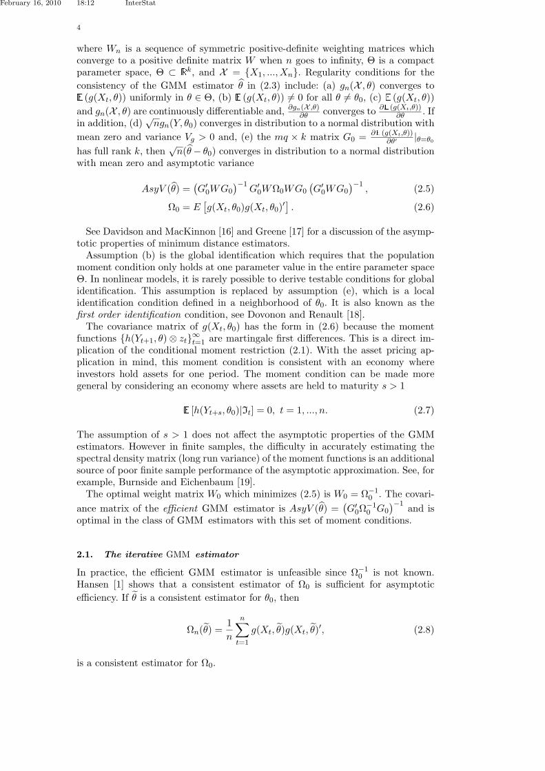
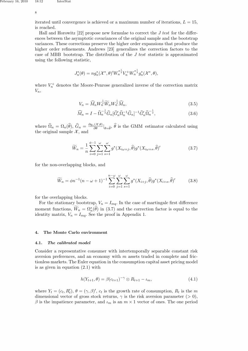
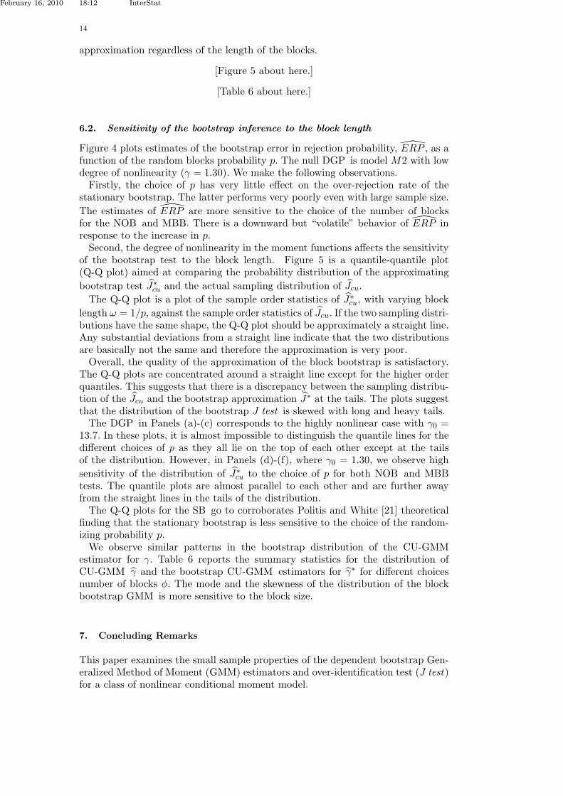
We further demonstrate these findings by a plot of the rejection probability,under the null model M2, as a function of p for nominal levels 5% and 10%. Theevidence in Figure 3 further supports the good performance of the NOB and MBB


14

approximation regardless of the length of the blocks.



6.2. Sensitivity of the bootstrap inference to the block length

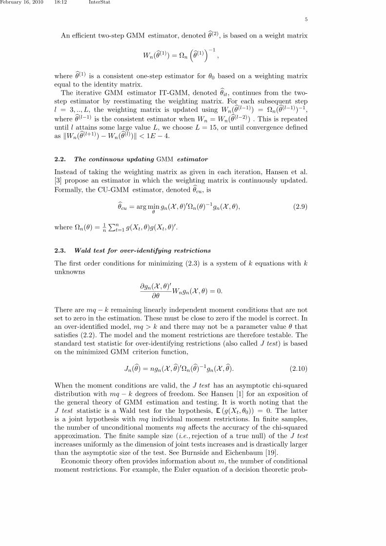
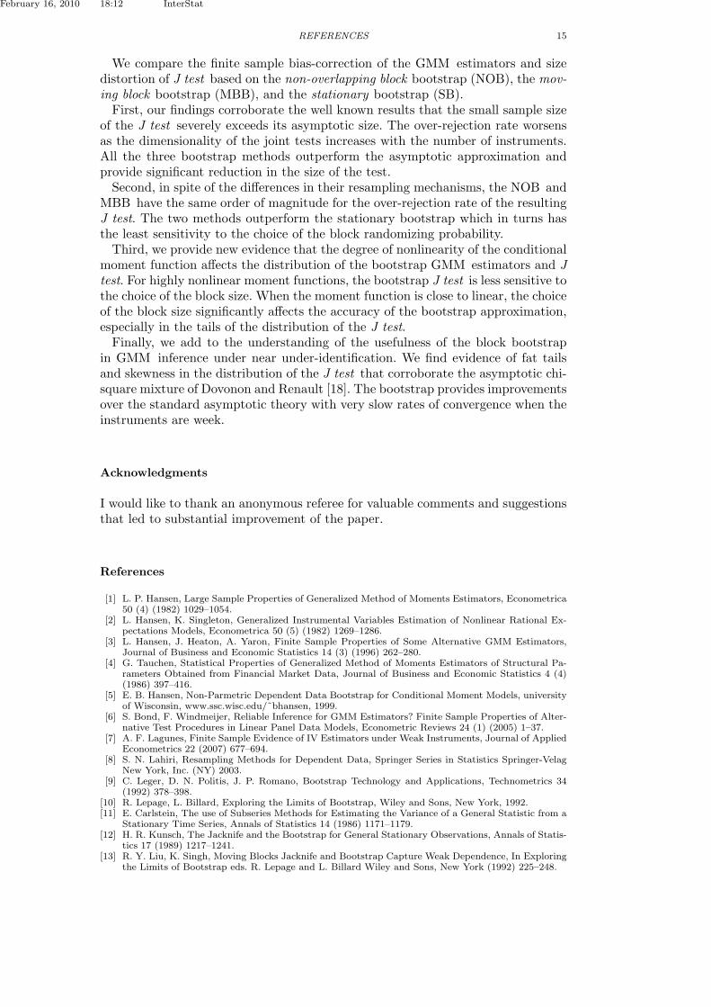
Figure 4 plots estimates of the bootstrap error in rejection probability, ERP , as afunction of the random blocks probability p. The null DGP is model M2 with lowdegree of nonlinearity (γ = 1.30). We make the following observations.

Firstly, the choice of p has very little effect on the over-rejection rate of thestationary bootstrap. The latter performs very poorly even with large sample size.The estimates of ERP are more sensitive to the choice of the number of blocksfor the NOB and MBB. There is a downward but “volatile” behavior of ERP inresponse to the increase in p.

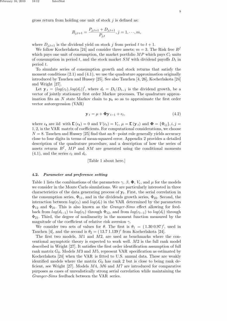
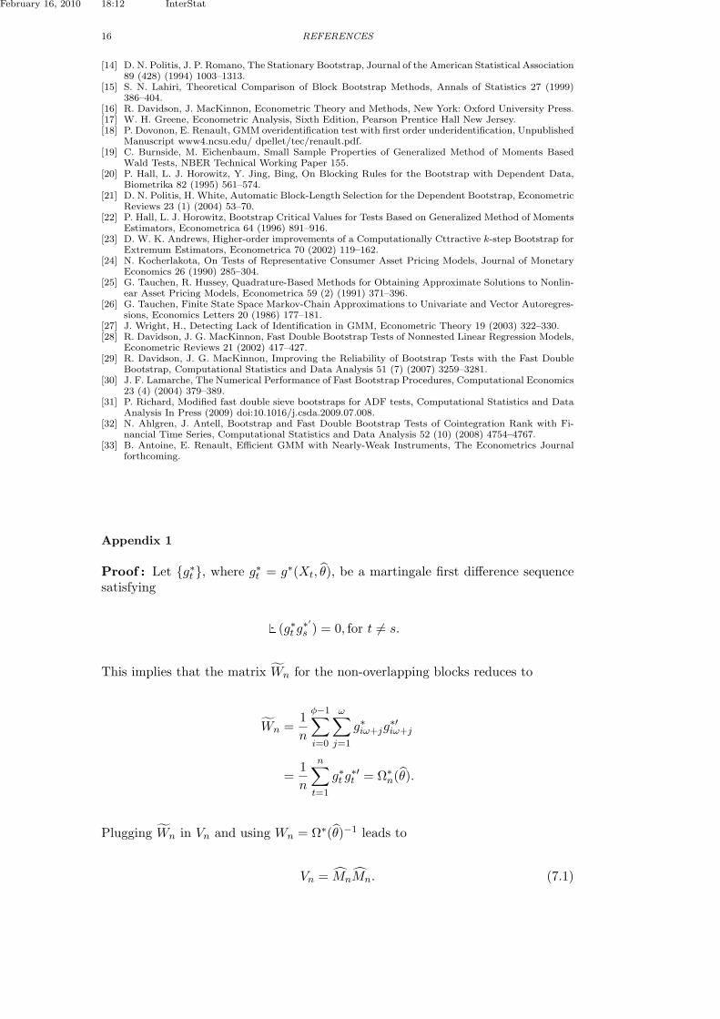
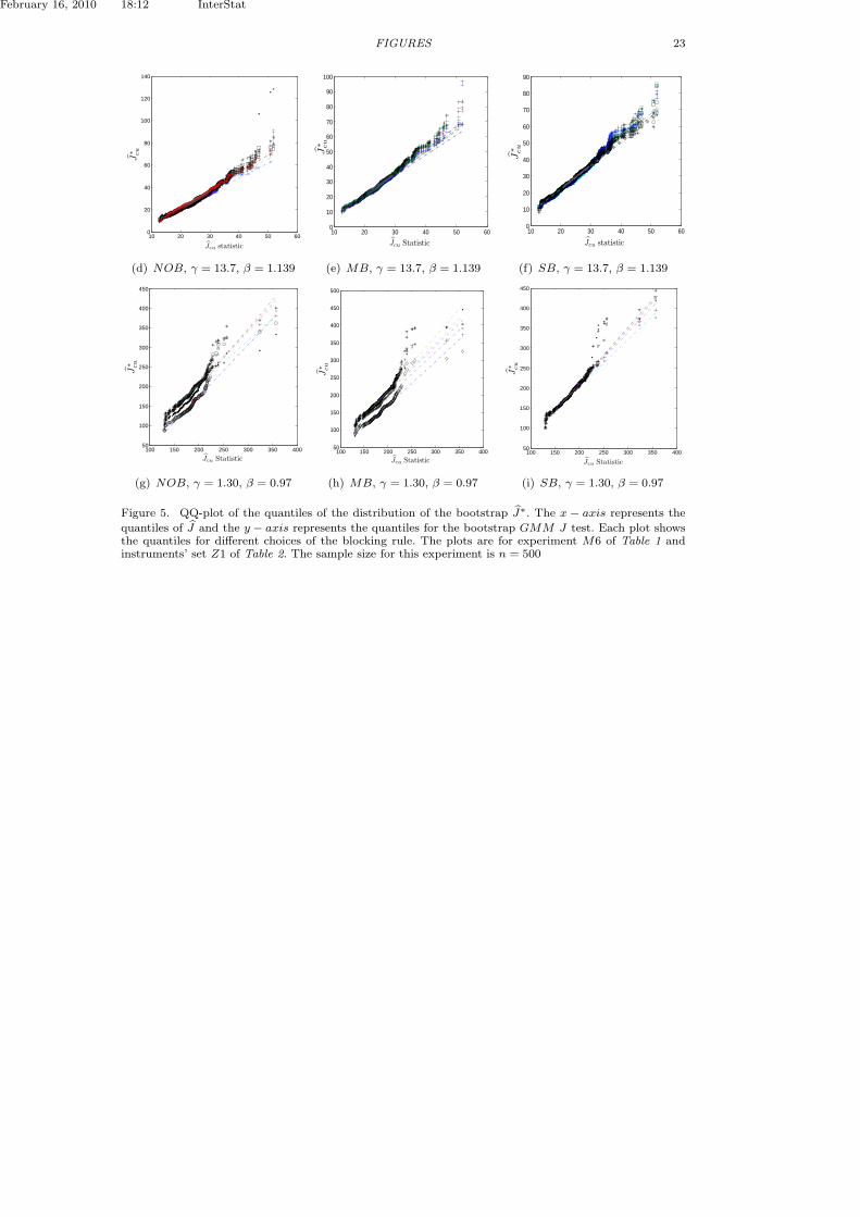
Second, the degree of nonlinearity in the moment functions affects the sensitivityof the bootstrap test to the block length. Figure 5 is a quantile-quantile plot(Q-Q plot) aimed at comparing the probability distribution of the approximatingbootstrap test J∗cu and the actual sampling distribution of Jcu.

The Q-Q plot is a plot of the sample order statistics of J∗cu, with varying blocklength ω = 1/p, against the sample order statistics of Jcu. If the two sampling distri-butions have the same shape, the Q-Q plot should be approximately a straight line.Any substantial deviations from a straight line indicate that the two distributionsare basically not the same and therefore the approximation is very poor.

Overall, the quality of the approximation of the block bootstrap is satisfactory.The Q-Q plots are concentrated around a straight line except for the higher orderquantiles. This suggests that there is a discrepancy between the sampling distribu-tion of the Jcu and the bootstrap approximation J∗ at the tails. The plots suggestthat the distribution of the bootstrap J test is skewed with long and heavy tails.

The DGP in Panels (a)-(c) corresponds to the highly nonlinear case with γ0 =13.7. In these plots, it is almost impossible to distinguish the quantile lines for thedifferent choices of p as they all lie on the top of each other except at the tailsof the distribution. However, in Panels (d)-(f), where γ0 = 1.30, we observe highsensitivity of the distribution of J∗cu to the choice of p for both NOB and MBBtests. The quantile plots are almost parallel to each other and are further awayfrom the straight lines in the tails of the distribution.

The Q-Q plots for the SB go to corroborates Politis and White [21] theoreticalfinding that the stationary bootstrap is less sensitive to the choice of the random-izing probability p.

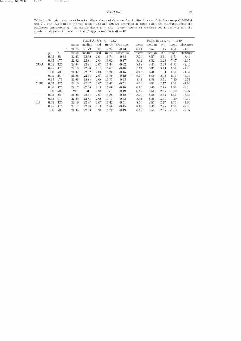
We observe similar patterns in the bootstrap distribution of the CU-GMMestimator for γ. Table 6 reports the summary statistics for the distribution ofCU-GMM γ and the bootstrap CU-GMM estimators for γ∗ for different choicesnumber of blocks φ. The mode and the skewness of the distribution of the blockbootstrap GMM is more sensitive to the block size.

7. Concluding Remarks

This paper examines the small sample properties of the dependent bootstrap Gen-eralized Method of Moment (GMM) estimators and over-identification test (J test)for a class of nonlinear conditional moment model.


REFERENCES 15

We compare the finite sample bias-correction of the GMM estimators and sizedistortion of J test based on the non-overlapping block bootstrap (NOB), the mov-ing block bootstrap (MBB), and the stationary bootstrap (SB).

First, our findings corroborate the well known results that the small sample sizeof the J test severely exceeds its asymptotic size. The over-rejection rate worsensas the dimensionality of the joint tests increases with the number of instruments.All the three bootstrap methods outperform the asymptotic approximation andprovide significant reduction in the size of the test.

Second, in spite of the differences in their resampling mechanisms, the NOB andMBB have the same order of magnitude for the over-rejection rate of the resultingJ test. The two methods outperform the stationary bootstrap which in turns hasthe least sensitivity to the choice of the block randomizing probability.

Third, we provide new evidence that the degree of nonlinearity of the conditionalmoment function affects the distribution of the bootstrap GMM estimators and Jtest. For highly nonlinear moment functions, the bootstrap J test is less sensitive tothe choice of the block size. When the moment function is close to linear, the choiceof the block size significantly affects the accuracy of the bootstrap approximation,especially in the tails of the distribution of the J test.

Finally, we add to the understanding of the usefulness of the block bootstrapin GMM inference under near under-identification. We find evidence of fat tailsand skewness in the distribution of the J test that corroborate the asymptotic chi-square mixture of Dovonon and Renault [18]. The bootstrap provides improvementsover the standard asymptotic theory with very slow rates of convergence when theinstruments are week.

Acknowledgments

I would like to thank an anonymous referee for valuable comments and suggestionsthat led to substantial improvement of the paper.

References

[1] L. P. Hansen, Large Sample Properties of Generalized Method of Moments Estimators, Econometrica50 (4) (1982) 1029–1054.

[2] L. Hansen, K. Singleton, Generalized Instrumental Variables Estimation of Nonlinear Rational Ex-pectations Models, Econometrica 50 (5) (1982) 1269–1286.

[3] L. Hansen, J. Heaton, A. Yaron, Finite Sample Properties of Some Alternative GMM Estimators,Journal of Business and Economic Statistics 14 (3) (1996) 262–280.

[4] G. Tauchen, Statistical Properties of Generalized Method of Moments Estimators of Structural Pa-rameters Obtained from Financial Market Data, Journal of Business and Economic Statistics 4 (4)(1986) 397–416.

[5] E. B. Hansen, Non-Parmetric Dependent Data Bootstrap for Conditional Moment Models, universityof Wisconsin, www.ssc.wisc.edu/˜bhansen, 1999.

[6] S. Bond, F. Windmeijer, Reliable Inference for GMM Estimators? Finite Sample Properties of Alter-native Test Procedures in Linear Panel Data Models, Econometric Reviews 24 (1) (2005) 1–37.

[7] A. F. Lagunes, Finite Sample Evidence of IV Estimators under Weak Instruments, Journal of AppliedEconometrics 22 (2007) 677–694.

[8] S. N. Lahiri, Resampling Methods for Dependent Data, Springer Series in Statistics Springer-VelagNew York, Inc. (NY) 2003.

[9] C. Leger, D. N. Politis, J. P. Romano, Bootstrap Technology and Applications, Technometrics 34(1992) 378–398.

[10] R. Lepage, L. Billard, Exploring the Limits of Bootstrap, Wiley and Sons, New York, 1992.[11] E. Carlstein, The use of Subseries Methods for Estimating the Variance of a General Statistic from a

Stationary Time Series, Annals of Statistics 14 (1986) 1171–1179.[12] H. R. Kunsch, The Jacknife and the Bootstrap for General Stationary Observations, Annals of Statis-

tics 17 (1989) 1217–1241.[13] R. Y. Liu, K. Singh, Moving Blocks Jacknife and Bootstrap Capture Weak Dependence, In Exploring

the Limits of Bootstrap eds. R. Lepage and L. Billard Wiley and Sons, New York (1992) 225–248.


16 REFERENCES

[14] D. N. Politis, J. P. Romano, The Stationary Bootstrap, Journal of the American Statistical Association89 (428) (1994) 1003–1313.

[15] S. N. Lahiri, Theoretical Comparison of Block Bootstrap Methods, Annals of Statistics 27 (1999)386–404.

[16] R. Davidson, J. MacKinnon, Econometric Theory and Methods, New York: Oxford University Press.[17] W. H. Greene, Econometric Analysis, Sixth Edition, Pearson Prentice Hall New Jersey.[18] P. Dovonon, E. Renault, GMM overidentification test with first order underidentification, Unpublished

Manuscript www4.ncsu.edu/ dpellet/tec/renault.pdf.[19] C. Burnside, M. Eichenbaum, Small Sample Properties of Generalized Method of Moments Based

Wald Tests, NBER Technical Working Paper 155.[20] P. Hall, L. J. Horowitz, Y. Jing, Bing, On Blocking Rules for the Bootstrap with Dependent Data,

Biometrika 82 (1995) 561–574.[21] D. N. Politis, H. White, Automatic Block-Length Selection for the Dependent Bootstrap, Econometric

Reviews 23 (1) (2004) 53–70.[22] P. Hall, L. J. Horowitz, Bootstrap Critical Values for Tests Based on Generalized Method of Moments

Estimators, Econometrica 64 (1996) 891–916.[23] D. W. K. Andrews, Higher-order improvements of a Computationally Cttractive k-step Bootstrap for

Extremum Estimators, Econometrica 70 (2002) 119–162.[24] N. Kocherlakota, On Tests of Representative Consumer Asset Pricing Models, Journal of Monetary

Economics 26 (1990) 285–304.[25] G. Tauchen, R. Hussey, Quadrature-Based Methods for Obtaining Approximate Solutions to Nonlin-

ear Asset Pricing Models, Econometrica 59 (2) (1991) 371–396.[26] G. Tauchen, Finite State Space Markov-Chain Approximations to Univariate and Vector Autoregres-

sions, Economics Letters 20 (1986) 177–181.[27] J. Wright, H., Detecting Lack of Identification in GMM, Econometric Theory 19 (2003) 322–330.[28] R. Davidson, J. G. MacKinnon, Fast Double Bootstrap Tests of Nonnested Linear Regression Models,

Econometric Reviews 21 (2002) 417–427.[29] R. Davidson, J. G. MacKinnon, Improving the Reliability of Bootstrap Tests with the Fast Double

Bootstrap, Computational Statistics and Data Analysis 51 (7) (2007) 3259–3281.[30] J. F. Lamarche, The Numerical Performance of Fast Bootstrap Procedures, Computational Economics

23 (4) (2004) 379–389.[31] P. Richard, Modified fast double sieve bootstraps for ADF tests, Computational Statistics and Data

Analysis In Press (2009) doi:10.1016/j.csda.2009.07.008.[32] N. Ahlgren, J. Antell, Bootstrap and Fast Double Bootstrap Tests of Cointegration Rank with Fi-

nancial Time Series, Computational Statistics and Data Analysis 52 (10) (2008) 4754–4767.[33] B. Antoine, E. Renault, Efficient GMM with Nearly-Weak Instruments, The Econometrics Journal

forthcoming.

Appendix 1

Proof : Let g∗t , where g∗t = g∗(Xt, θ), be a martingale first difference sequencesatisfying

E (g∗t g∗′s ) = 0, for t 6= s.

This implies that the matrix Wn for the non-overlapping blocks reduces to

Wn =1n

φ−1∑

i=0

ω∑

j=1

g∗iω+jg∗′iω+j

=1n

n∑

t=1

g∗t g∗′t = Ω∗n(θ).

Plugging Wn in Vn and using Wn = Ω∗(θ)−1 leads to

Vn = MnMn. (7.1)


REFERENCES 17

Let Mn = Imq − Pn where Pn = Ω− 1

2n Gn[G′nΩ−1

n Gn]−1G′nΩ− 1

2n . Pn is an idempotent

matrix, that is Pn = P ′n and Pn = PnPn. Therefore,

Vn = MnMn

= Imq − Pn + PnPn = Imq

Appendix 2: Quadrature approximation

The Euler equation for the calibrated economy can be written in terms of pricesand dividends,

Eθ

[βc−γt+1(1 + vt+1)dt+1

∣∣ It]

= vt (7.2)

where we denote by dt = DtDt−1

the dividend growth, vt = PtDt

the price-dividend

ratio and ct = Ct+1

Ctthe consumption growth.

Our economy is similar to the one described by Kocherlakota [24] with threeassets: the Risk free Rf which pays one unit of consumption, the market portfolioMP which pays Ct in period t and the stock market SM with dividend payoffs Dt

in period t. Equation (7.2) implies a conditional moment restriction for each assetj ∈ MP,SM,Rf.

The only driving random processes in the model are ct and dt, and so, conditionalon the past, Pt, or equivalently, vt is a deterministic function of ct and dt implicitlygiven by the Euler equation (7.2).

The deterministic function that gives vt as a solution to (7.2) cannot be foundin closed analytic form. The quadrature approximation uses a finite state Markovprocess to approximate the bivariate vector autoregression, and enables the ap-proximate solution to be obtained by matrix inversion.

The approximation involves fitting a 8 state Markov chain to log consumptiongrowth and log dividend growth calibrated so as to approximate the first orderVAR in (4.2).

Let c(l) and d(l), l = 1, ..., 16, denote the abscissa for the 8 − point quadraturerule. Each combination of abscissa (k, k′), k = 1, .., 8; k′ = 1, ..., 8 defines a statesj , for j = 1, ..., N , where N = 82. Let csj and dsj denote the values of c and d instate sj and let Ysj = (csj , dsj ).

The transition matrix Π for the Markov process defined by Πk,j =P(Yt+1 = ysj |Yt = ysk

)where,

Πk,j =p(ysj |ysk)S(ysk)p(ysj )

wj (7.3)

where S(x) =∑N

l=1p(ysl |x)

p(ysl )wl. The Gaussian rule defines p(x|ysk) and p(x) as den-

sity functions for the bi-variate normalsN(ysk ,Σ) andN(µ,ΣY ) respectively, whereΣY solves ΣY = ΦΣY Φ′+Σ. The weights wj are computed using a Hermite Gaussrule.

The solution to the integral in the Euler equation (7.2) is characterized by thesolution to the system of N linear equations given by the discrete approximation


18 REFERENCES

in

βN∑

j=1

Πk,j(csj )−γ(1 + vsj )dsj = vsk k = 1, .., N (7.4)

The solution exists if all the eigenvalues of the N × N matrix S defined by theelements Sk,j = βΠk,j(csj )−γ dsj lie within the unit circle. The solution is charac-terized by,

v = (IN − S)−1SιN (7.5)

where ιN is a N × 1 column vector of ones. For the market portfolio, the dividendratio is equal to dMP,sj = csj and therefore Sk,j = βΠk,j(csj )1−γ . From the seriesof the equilibrium price-dividend ratios vi, i ∈ F,MP, SM, the correspondingreturns are computed as:

rMP,sksj = csj1 + vMP,sj

vMP,sk

rSM,sksj = dsj1 + vSM,sj

vSM,sk

rF,sk = 1/

T∑

j=1

βΠk,j(csj )−γ

See, for example, Tauchen [26], Tauchen and Hussey [25] and Kocherlakota [24] forfurther details about these derivations.


FIGURES 19

0 20 40 60 80 1000

0.01

0.02

0.03

0.04

0.05

0.06

0.07

0.08

0.09

0.1

Jcu, M6, n = 120

Jcu, M5, n = 120

χ210

Jcu, M1, n = 120

(a) Granger-Sims effect, case of Z = Z1

0 20 40 60 80 1000

0.01

0.02

0.03

0.04

0.05

0.06

0.07

0.08

0.09

0.1

Jcu, M5, n = 120

Jcu, M3, n = 120

χ210

(b) Nonlinearity effect, case of Z = Z1

0 20 40 60 80 1000

0.01

0.02

0.03

0.04

0.05

0.06

0.07

0.08

0.09

0.1

χ210

Jcu, M2, n = 120

Jit, M2, n = 120

(c) Choice of weight matrix Wn, case of Z = Z1

0 10 20 30 40 500

0.02

0.04

0.06

0.08

0.1

0.12

0.14

0.16

0.18

0.2

Jcu, M4, n = 120

Jcu, M3, n = 120χ2

4

(d) Serial correlation Effect, case of Z = Z2

Figure 1. Kernel density estimate for the sampling distribution of the J test statistic, J , where Jit is

for the IT-GMM and, Jcu is for the CU-GMM. The sample size is n = 120, the number of Monte Carlosimulations is M = 10, 000. Z1 and Z2 are the instruments used in the estimation. The plots also showthe asymptotic χ2

df probability density, where df is the number of degrees of freedom.


20 FIGURES

0 0.02 0.04 0.06 0.08 0.1 0.12 0.14 0.16 0.18 0.20

0.1

0.2

0.3

0.4

0.5

0.6

0.7

0.8

Nominal Size, α

RP

A

NOB

MBB

SB

χ2df

45 − line

(a) n = 120, Z = Z3, df = 1

0 0.02 0.04 0.06 0.08 0.1 0.12 0.14 0.16 0.18 0.20

0.1

0.2

0.3

0.4

0.5

0.6

0.7

0.8

0.9

1

Nominal Size, α

RP

A

NOB

MBB

SB

45 − line

χ2df

(b) n = 120, Z = Z4, df = 7

0 0.02 0.04 0.06 0.08 0.1 0.12 0.14 0.16 0.18 0.20

0.1

0.2

0.3

0.4

0.5

0.6

0.7

Nominal Size, α

RP

A

NOB

MBB

SB

χ2df

45 − line

(c) n = 500, Z = Z3, df = 1

0 0.02 0.04 0.06 0.08 0.1 0.12 0.14 0.16 0.18 0.20

0.1

0.2

0.3

0.4

0.5

0.6

0.7

0.8

0.9

1

Nominal Size, α

RP

A

NOB

MBB

SB

χ2df

45 − line

(d) n = 500, Z = Z4, df = 7

Figure 2. Fast Bootstrap estimate of the rejection probability approximation, RPA, for the bootstrapCU-GMM J test under the null model M2. Each bootstrap method is represented by a different line-style,and each line represents a specific choice of the block length ω = 1/p, where p = 0.05, 0.10, 0.15, · · ·, 1. Therejection probability for the asymptotic J test is represented by the χ2

df line, where df is the number of

degrees of freedom.


FIGURES 21

0 0.2 0.4 0.6 0.8 10

0.01

0.02

0.03

0.04

0.05

0.06

p = 1/ω

NOB

MBB

SB

Nominal α

(a) n = 500, Z3

0.2 0.4 0.6 0.8 10

0.01

0.02

0.03

0.04

0.05

0.06

0.07

0.08

0.09

0.1

p = 1/ω

NOB

MBB

SB

Nominal , α

(b) n = 500, Z3

0 0.2 0.4 0.6 0.8 1

0.05

0.1

0.15

0.2

0.25

0.3

0.35

0.4

0.45

p = 1/ω

NOBMBBSBNominal α

(c) n = 500, Z4

0 0.2 0.4 0.6 0.8 1

0.05

0.1

0.15

0.2

0.25

0.3

0.35

0.4

0.45

0.5

0.55

p = 1/ω

NOB

MBB

SB

Nominal α

(d) n = 500, Z4

Figure 3. Bootstrap approximation for the error in rejection probability, ERP (α) for α = 0.05, Fig 3aand Fig 3c, and α = 0.10, Fig 3b and Fig 3d. The null DGP is M2 with γ0 = 1.30 and β = 0.97. Thesample size is n = 500, Z3 and Z4 are defined in Table 2.


22 FIGURES

Figure 4. Estimates of the error in the rejection probability, ERP for the bootstrap GMM test, J∗cu as a

function of the block size, ω, where ω = 1p

and nominal size α. The null model is model M2, instruments

are Z = Z4 and sample size n = 500.

(a) SB (b) MBB (c) NOB


FIGURES 23

10 20 30 40 50 600

20

40

60

80

100

120

140

Jcu statistic

J∗ cu

(d) NOB, γ = 13.7, β = 1.139

10 20 30 40 50 600

10

20

30

40

50

60

70

80

90

100

Jcu Statistic

J∗ cu

(e) MB, γ = 13.7, β = 1.139

10 20 30 40 50 600

10

20

30

40

50

60

70

80

90

Jcu statistic

J∗ cu

(f) SB, γ = 13.7, β = 1.139

100 150 200 250 300 350 40050

100

150

200

250

300

350

400

450

Jcu Statistic

J∗ cu

(g) NOB, γ = 1.30, β = 0.97

100 150 200 250 300 350 40050

100

150

200

250

300

350

400

450

500

Jcu Statistic

J∗ cu

(h) MB, γ = 1.30, β = 0.97

100 150 200 250 300 350 40050

100

150

200

250

300

350

400

450

Jcu Statistic

J∗ cu

(i) SB, γ = 1.30, β = 0.97

Figure 5. QQ-plot of the quantiles of the distribution of the bootstrap J∗. The x − axis represents the

quantiles of J and the y − axis represents the quantiles for the bootstrap GMM J test. Each plot showsthe quantiles for different choices of the blocking rule. The plots are for experiment M6 of Table 1 andinstruments’ set Z1 of Table 2. The sample size for this experiment is n = 500


24 TABLES

Table 1. Parameter and preference settings for the Monte Carlo experiments. The DGP is calibrated using the

risk aversion parameter γ and the discount factor β. The consumption and dividends growth series are calibrated

using a VAR with mean µ, matrix coefficient Φ and error covariance matrix Vε.

Model γ β Φ Vε µ

M1 13.7 1.139

(−.50 0

0 −.50

) (.01 .00.00 .01

) (.00.00

)

M2 1.30 .97

(−.50 0

0 −.50

) (.01 .00.00 .01

) (.00.00

)

M3 1.30 .97

(−.161 .017.414 .117

) (.00120 .00177.00177 .01400

) (0.0210.004

)

M4 1.30 .97

(−.677 .017.414 .117

) (.00120 .00177.00177 .01400

) (0.0210.004

)

M5 13.7 1.139

(−.161 .017.414 .117

) (.00120 .00177.00177 .01400

) (0.0210.004

)

M6 13.7 1.139

(−.677 .017.414 .117

) (.00120 .00177.00177 .01400

) (0.0210.004

)

M7 13.7 1.139

(−.85 .414.03 −.50

) (.00120 .00177.00177 .01400

) (0.0210.004

)

M8 1.30 .97

(−.85 .414.03 −.50

) (.00120 .00177.00177 .01400

) (0.0210.004

)


TABLES 25

tTable 2. Variables used in the GMM estimation of the Calibrated economy

Returns Rt Instruments Zt df

Z1t rft−1, rMPt−1 , r

SMt−1 1, ct−1, r

ft−1, r

MPt−1 , r

SMt−1 10

Z2t rft−1, rMPt−1 , r

SMt−1 1, ct−1 4

Z3t rSMt−1 1, ct−1 1

Z4t rSMt−1 1, ct−1, ct−2, ct−3, ct−4 7


26 TABLES

Table 3. Sample mean, sample median, sample mode, standard deviation (std) and sample skewness of the dis-

tribution of J test for the iterated and the continuously updated GMM. The number of Monte Carlo replications

is M = 10, 000, df is the number of degrees of freedom of the asymptotic χ2 test and the sample size is n = 120.

The null DGP of experiments M3, M4 and M6 is described in Table 1. For the asymptotic test, the mean,

median, standard deviation, mode and skewness correspond to their theoretical values for a χ2df .

CU-GMM, Jcu IT-GMM, Jit

df = 10 df = 4 df = 10 df = 4 Asymptotic test

M6 M3 M6 M4 M6 M4 M6 M4 χ210 χ2

4

mean 41 27 18 42 91 64 42 181 10 4median 40 20 17 40 90 61 40 180 9.34 3.36std 12 19 6 13 20 17 15 25 4.47 2.82mode 13 5 6 11 39 23 8 105 8 2skewness 0.73 1.77 1.09 1.00 0.53 0.91 0.51 0.29 0.89 1.41


TABLES 27

Table 4. Measures of Bias and performance for GMM estimators of γ and β. Case of Continuous updating

estimator, n = 120

A: Effect of VAR specification B: Effect of sample sizeInstruments, Z1, df = 10 Instruments, Z2, df = 4

true γ0 = 13.7, β0 = 1.139 true γ0 = 13.7, β0 = 1.139

n = 120 Model: M6

M7 M1 M5 n = 120 n = 500

γ β γ β γ β γ β γ β

mean 21.114 1.188 14.964 1.262 15.990 1.202 15.990 1.2026 15.470 1.198median 21.776 1.184 14.779 1.264 15.713 1.200 15.713 1.2004 15.437 1.199

std 2.922 0.053 1.225 0.099 1.689 0.036 1.689 0.0366 0.574 0.015RMSE 7.969 0.072 1.760 0.158 2.846 0.073 3.660 0.0636 1.801 0.059


28 TABLES

Table 5. Sample measures of location, dispersion and skewness for the distribution of the bootstrap CU-GMM

test J∗. The DGPs under the null models M3 and M4 are described in Table 1 and are calibrated using the

preference parameters θ0. The sample size is n = 120, the instruments Z1 and Z2 are described in Table 2,

and df is the number of degrees of freedom of the χ2 approximation. The number of nonrandom blocks for

NOB and MBB is φ = n/ω, where the blocks length ω is ω = 1/p and p is the stationary bootstrap probability,

p = 0.05, 0.10, ···, 1. For comparison, the last row in each Panel reports the summary statistics for the distribution

of CU-GMM test, Jcu.

Panel A: Null model is M3, Z = Z1, df = 10, θ0 = (1.30, 0.97)′

Non-overlapping blocks: NOB Moving blocks: MBB Stationary bootstrap: SBp = 1/ω φ = n/ω mean median mode std skewness mean median mode std skewness mean median mode std skewness0.05 6 40 28 5 28 1.26 42 31 3 28 1.23 48 37 6 30 1.060.15 18 43 30 2 31 1.53 45 33 8 30 1.15 48 37 4 29 1.030.25 30 45 32 5 32 2.21 46 34 5 30 1.24 48 36 7 29 0.980.35 42 46 35 4 30 1.20 46 34 3 30 1.16 47 36 5 29 1.020.45 54 46 35 5 30 1.18 47 35 8 30 1.10 48 36 7 29 1.080.55 66 47 35 3 29 1.12 47 36 4 29 1.03 48 37 7 29 0.950.65 78 47 36 7 30 1.06 47 36 5 29 1.06 49 38 6 30 1.010.75 90 47 37 4 29 1.12 47 36 3 29 0.98 48 36 7 29 0.970.85 102 48 36 4 30 1.12 48 36 6 30 1.02 47 37 8 29 0.991.00 120 48 37 7 30 1.01 48 36 2 30 0.99 48 37 6 29 0.98

Jcu 27 20 5 19 1.77

Panel B: Null model is M6, Z = Z1, df = 10, θ0 = (13.7, 1.139)′


Jcu 41 40 13 12 0.73

Panel C: Null model is M3, Z = Z2, df = 4, θ0 = (1.30, 0.97)′


Panel D: Null model is M6, Z = Z2, df = 4, θ0 = (13.7, 1.139)′


Jcu 18 17 6 6 1.09


TABLES 29

Table 6. Sample measures of location, dispersion and skewness for the distribution of the bootstrap CU-GMM

test J∗. The DGPs under the null models M3 and M6 are described in Table 1 and are calibrated using the

preference parameters θ0. The sample size is n = 500, the instruments Z1 are described in Table 2, and the

number of degrees of freedom of the χ2 approximation is df = 10.

Panel A: M6, γ0 = 13.7 Panel B: M3, γ0 = 1.139mean median std mode skewness mean median std mode skewness

γ 21.75 21.79 1.87 17.24 -0.13 8.51 8.54 1.16 1.30 -1.10p φ mean median std mode skewness mean median std mode skewness

NOB

0.05 25 22.03 22.59 2.04 16.74 -0.24 8.39 8.57 2.11 -8.71 -3.460.35 175 22.02 22.81 2.04 16.02 -0.47 8.42 8.52 2.29 -7.67 -2.150.65 325 22.04 22.81 2.07 16.44 -0.62 8.08 8.47 2.66 -8.71 -2.440.95 475 22.18 22.86 2.17 16.67 -0.48 7.91 8.32 3.13 1.30 -1.731.00 500 21.97 22.62 2.06 16.20 -0.45 8.35 8.46 1.93 1.30 -1.34

MBB

0.05 25 21.96 22.51 2.07 15.89 -0.42 8.30 8.59 2.33 1.30 -3.360.35 175 22.05 22.83 2.06 15.73 -0.53 8.41 8.59 2.51 -7.19 -0.550.65 325 22.19 22.87 2.07 16.42 -0.51 8.20 8.53 2.77 1.30 -1.900.95 475 22.17 22.96 2.16 16.56 -0.45 8.09 8.43 2.75 1.30 -2.181.00 500 22 23 1.98 17 -0.49 8.22 8.53 2.65 -7.59 -2.07

SB

0.05 25 21.96 22.51 2.07 15.89 -0.42 8.30 8.59 2.33 1.30 -3.360.35 175 22.05 22.83 2.06 15.73 -0.53 8.41 8.59 2.51 -7.19 -0.550.65 325 22.19 22.87 2.07 16.42 -0.51 8.20 8.53 2.77 1.30 -1.900.95 475 22.17 22.96 2.16 16.56 -0.45 8.09 8.43 2.75 1.30 -2.181.00 500 21.95 22.53 1.98 16.79 -0.49 8.22 8.53 2.65 -7.59 -2.07

finite sample properties of bootstrap gmm for nonlinear conditional moment...

Documents