Journal of Econometrics 32 (1986) 333-366. North-Holland

FINITE-SAMPLE PROPERTIES OF THE INSTRUMENTAL-VARIABLES ESTIMATOR FOR DYNAMIC

SIMULTANEOUS-EQUATION SUBSYSTEMS WITH ARMA DISTURBANCES *

Julia CAMPOS

Bunco Central de Venezuela, Curacus, Venezuelu

Received November 1983, final version received January 1986

Monte Carlo methods are proposed and implemented for studying the finite-sample bias, standard error and estimated asymptotic standard error of the instrumental-variables estimator (IVARMA) of incomplete dynamic simultaneous-equation systems with ARMA disturbances. A control variate is derived for constructing efficient Monte Carlo estimators of the finite-sample moments of IVARMA and response surfaces are developed to obtain approximations to the finite-sample moment functions.

1. Introduction

Full-information maximum likelihood is appealing for estimating dynamic simultaneous-equation systems in econometrics: under weak assumptions, the estimator is consistent and asymptotically efficient and utilizes all overidentify- ing restrictions in the system. However, limited-information methods may be preferable when, e.g., the sample size is small, the number of predetermined variables is large, the specification of part of the system is in question, or

computational costs are a consideration. Further, maximum-likelihood estima- tion as such may be inconsistent if the system is non-linear in its parameters and the disturbances are incorrectly assumed to be normally distributed, whereas instrumental-variables methods rely on weaker assumptions about the distribution of the disturbances. Sargan (1958,1959) derives the asymptotic properties of the instrumental-variables estimator when the errors either are

*An earlier version of this paper was presented at the European Meeting of the Econometric Society (Pisa, 1983); more detailed results appear in my Ph.D. thesis at the London School of Economics [Campos (1982)]. I wish to thank J.D. Sargan, D.F. Hendry, N.R. Ericsson, M. Knott, R. Campos. R. Chapmam and a referee for helpful advice and comments. I gratefully acknowl- edge financial support from the Venezuelan Studentship Programme Fundacibn Gran Mariscal de Ayacucho and from the Social Science Research Council to the Programmes in Quantitative Economics and in Methodology, Inference and Modelling in Econometrics at the London School of Economics. The views expressed in this paper do not necessarily reflect those of the Banco Central de Venezuela.

0304.4076/86/$3.500 1986, Elsevier Science Publishers B.V. (North-Holland)

334 J. Campos, Properties of the instrumental-vanahies estimator

independent and identically distributed or follow an autoregressive scheme: its finite-sample properties have been examined using both analytic and Monte Carlo methodologies. Campos (1986) expands upon Sargan’s results, propos- ing an instrumental-variables estimator (IVARMA) of possibly incomplete dynamic simultaneous-equation systems with autoregressive moving-average (ARMA) disturbances and deriving its asymptotic properties. As is apparent from the literature on econometric estimators, appreciable discrepancies may

exist between their finite-sample and asymptotic properties: understanding the nature of those discrepancies can aid applied econometricians in assessing the value of those estimators. This paper examines the finite-sample properties of the IVARMA estimator by using Monte Carlo methods to derive numer- ical-analytical representations of the moment functions of that estimator.

Section 2 defines the system and gives the IVARMA estimator and its asymptotic properties. Section 3 motivates the methodology developed in the following sections. In section 4, a control variate (CV) for estimating the first two moments of IVARMA is derived in order to construct efficient Monte Carlo estimators of its finite-sample moments. Sections 5, 6 and 7 derive the functional forms of response surfaces for IVARMA’s finite-sample bias, standard error and estimated asymptotic standard error. In section 8, a two-equation data-generation process with ARMA (1,l) disturbances is chosen for studying the effects of autocorrelation, dynamics and sample size on the finite-sample properties of IVARMA. For that data-generation process, the exact asymptotic variance-covariance matrix (appendices B and C) is ob- tained. Finally, section 9 gives the Monte Carlo results in the form of response surfaces and presents the efficiency gains from using Monte Carlo estimators based on the CV rather than from using naive Monte Carlo estimators.

2. The instrumental-variables estimator IVARMA

We consider instrumental-variables estimation of parameters from systems of the following kind:

E * - i.i.d.(O, 52) t=l,...,T,

where B(L), C(L), R(L) and S(L) are N X n, N X m, N X N and N X N matrices of polynomials of finite orders in the lag operator L. yr is a vector of n endogenous variables (n 1 N), z, is a vector of m exogenous variables, u, is

an N x 1 vector of ARMA errors associated with the structural equations and Ed is an N x 1 vector of innovations with E(E&) = 9. It is assumed that

J. Cumpos, Properties of the Instrumental-variables estmutor 335

det( R( L)) = 0 and det( S( L)) = 0 have their roots outside the unit circle and that the system is identified.

Assuming that there are (1 unknown parameters in the matrices of poly- nomials and denoting that vector of parameters by 8, the IVARMA esti- mator fi can be regarded as that obtained by minimizing the function A (8) = tr[d-‘(.?(e)Z*)(Z*~Z*)-‘(Z*‘E(@))] with respect to 8, where fi is a con- sistentestimatorof 0, EistheTXNmatrix(ei,...,+)‘,and Z*isa TXm* matrix of instrumental variables of rank m*. Under suitable conditions, Campos (1986) shows that

plim 8 = (3, and T'/2(& &,) - N(O,E), u

where &, is the vector of true parameter values, and

2 = plim[ QGQ’] -l,

with

Q= T-l[e(vec&')'/ae]le,(l,~Z*),

and

G=k'@(Z*'Z*/T)-'.

2 can be consistently estimated by using the same expression evaluated at the estimated values. [Cf. Bowden and Turkington (1984).]

3. Methodologies for investigating finite-sample properties of econometric estimators

The choice of an estimation method is based in part on the properties of the estimator’s finite-sample distribution. However, deriving exact distributions is

often a difficult problem, particularly if the classical assumptions (i.e., non-sto- chastic predetermined variables and normally distributed disturbances) are not satisfied. Hence, exact distributions generally have been obtained assuming that the equation has no lagged endogenous variables and that the errors are independent and normally distributed. Also, very often those exact densities are expressed in terms of multiple infinite series which may be difficult to interpret, whose convergence may be slow and which may be difficult to compute. [See Phillips (1980).]

The asymptotic distribution of an econometric estimator may not be very good as an approximation to its finite-sample distribution for some models, in some regions of the parameter space and for sample sizes often available to econometric studies of time series. Thus, in cases where the exact finite-sample

336 J. Campos, Properties of the instrumentul-variables estlmutor

distribution is intractable, analytic approximations have been derived for some estimators. See, for instance, Sargan (1976) whose derivation allows for lagged endogenous variables and in some cases for non-normal errors. However, the formulae can be very complicated because the number of terms in each of the coefficients of the Edgeworth expansion increases rapidly with the number of parameters in the model. Analytic approximations to the finite-sample mo- ments of some econometric estimators have also been obtained [see, for instance, Nagar (1959)]. Monte Carlo methods also have been used to estimate

the first two finite-sample moments of some econometric estimators. [See among others Hendry and Srba (1977).] However, there are some disad- vantages in using Monte Carlo simulation rather than purely analytic methods [see Hendry (1984)]: Monte Carlo results can be imprecise and specific. Those problems can be overcome at least in part to produce valid and fairly general results. Imprecision can be reduced by using a large number of replications and/or by variance-reduction techniques since Monte Carlo estimators with smaller standard errors can be constructed. The analysis of the simulation results by regression methods can increase the generality of the Monte Carlo study. The remainder of this section develops the theory for those techniques.

Antithetic variates and control variates provide variance-reduction tech- niques that can be used in econometrics. Both are based on the construction of a statistic which is a function of a naive (i.e., direct) Monte Carlo estimator of a parameter and of an additional estimator highly correlated with the naive one. [Antithetic variates are not considered further in this paper; see Hendry (1984).] The CV is usually defined as a statistic 8* positively correlated with the econometric estimator under study (0) and whose exact finite-sample distribution is known. However, the control variate for estimating the first two moments of the estimator fi can be defined more conveniently as an economet- ric estimator whose first two moments are known exactly and which is asymptotically equivalent to 6. Assuming’ that fi is consistent and that 8* is unbiased for S,, the knowledge of E( 8 * ) and E[ 8 * - E( 8 *)] 2 and the asymp: totic equivalence of 8* to 8 allow for decomposing the first two moments of 8 into a known term [either E( 0*) or E[8* - E(e*)]2] and an unknown term which is the expectation of terms of oP(TP’/‘). Hence, instead of simulating

expectations of terms of 0P(T-‘/2), we simulate expectations of terms of o,(T-l/*). Such Monte Carlo estimators for the bias and variance of & (the i th element of B) can be constructed as follows.

The naive Monte Carlo estimator of the bias of 6, is

&r,=J-l 5 (ej-&,), ;=1

’ Notice that consistency of e and unbiasedness of O* are not required for this result to follow for the first moment of e.

J. Campos, Properties of the instrumental-uariahl estimutor 337

where 8jj is the value of the econometric estimator of the i th parameter in the jth replication and J is the number of replications. I$~, is an unbiased estimator of the bias of 8, and has a variance of O(J-I). That variance is the variance of a term 0p(T-1/2). A Monte Carlo estimator based on the CV can

be defined by

where l?,T is the CV estimate of the ith parameter in the jth replication. A pooled estimator of the bias of 8, can be constructed as

It follows that the first two moments of the pooled estimator are

WL) = EM - 4,) and var($,,) =J-‘V(g,-8:).

That is, the pooled estimator is unbiased for the finite-sample bias of 8,; and

its variance is of the same order in the number of replications as the variance of the naive estimator, but is the variance of a term of smaller order in the econometric sample size than that of the naive estimator [i.e., o,(T-‘/~)

instead of O,( T-‘/*)1.

Similarly, a naive Monte Carlo estimator for the variance of 6, can be defined as

iJ2r=(J-1)-1 i (t9,,-8,j2=SSD,Z (say), /=I

where

Using the CV, a Monte Carlo estimator is

I//;,=(J-~)-~ i (6’,T-8;*)2 with ai* = J-’ i 8,: j=l i=l

The pooled estimator of the variance of 8; is

&;=(J-l)-l i [(8,-8)2-(B,;-@)2] +E[8,*-E(0:)]2,

j=l

33x J. Cumpos, Properties of the instrumentul-vuricrhles estimator

which is an unbiased estimator of the variance of the IVARMA estimator, and whose variance is the variance of a term of o,(T-‘) [instead of O,(T-‘) as in the case of $,,I.

The efficiency gain from using a CV can be calculated as the ratio of the variance of the naive estimator to that of the pooled estimator.

The finite-sample moments of econometric estimators, if they exist, are often unknown functions of the econometric sample size and the parameters of the data-generation process. In the experimental design literature, those functions are called response functions and the objective of the Monte Carlo study may be to estimate them, thereby obtaining numerical-analytical repre- sentations of the moment functions. Those approximating functions are re- sponse surfaces [see Hendry and Srba (1977) for a formal definition] and asymptotic theory can guide their construction by determining the order (in T) of the terms in the response surface. After estimation, the specification of the response surface can be tested. A significant difference between the error variances of the response surface and the true function, the presence of autocorrelation and heteroscedasticity in the residuals and predictive failure are all evidence of mis-specification. Below, several test statistics are used to check against specification errors. In addition to approximating the moment functions, response surfaces may usefully summarize the results and reduce the specificity of the Monte Carlo study since predictions of the response can be obtained for other points in the experimental region.

4. A control variate for the bias and standard error of IVARMA

The CV estimator is a member of the class of estimators defined by the estimator-generating equation. The estimator-generating equation of IVARMA for model (1) is given by

T-1[~Z~(e)/~e~e~](,++~1/2(8- e,) = -T-lq~A(e)/ae] lo,,

where r3++ hes on the line segment joining 8 and do. Thus, letting Q+ = plim Q and G’ = plim G, the CV estimator is defined as

e* =e,- T-12Q+G+(l,@Z*')vec~'; (2) and assuming that the process generating ( y,, z,) and Z * is ergodic, its mean is E( t9*) = B,, its variance-covariance matrix is given by E(8* - e,)( 8* - 0,)’ = T-‘2, and g - O* = o,(T-‘/~) (see appendix A). In (2), 2 is the asymptotic variance-covariance matrix (AVM) of IVARMA, Q’ and G+ can be obtained from the formulae used in calculating the AVM, and the last term involves the instruments and the disturbances, whose values are known in the Monte Carlo study. Using this CV, pooled estimators of the bias and variance of IVARMA

J. Gwnpos, Properties of the instrumentul-variables estimator 339

can be constructed and they can provide substantially more precise estimates

of the bias and the variance than the corresponding naive Monte Carlo estimators.

5. The functional form of response surfaces for the biases

To analyse the finite-sample bias of IVARMA as a function of the sample size T and the parameters of the data-generation process, the moment function HL(q, T) is estimated, where

and ‘p includes all the parameters of the complete system and those which define the data-generation process of z,. E(g, - da,) is unknown, but can be accurately estimated by the naive Monte Carlo estimator of the finite-sample bias. Hence (3) may be estimated by the response surface &irk = Hc+(cp,, T,)

+ ‘G (k = 1,. _. , K), where a variable with the subscript k denotes that variable in the k th experiment, K is the number of experiments,* HL( .) is a function approximating HG( .), and hL.+ is a composite error arising from the error in estimating E(B - t9,,,) by qii, and the error in approximating the moment function. For simplicity of notation, the subscript k is dropped.

Asymptotic theory is used in specifying the functional form of HL+( .). Because Hz+( .) IS non-stochastic, f?, is consistent for B,,, and T”“(8 - 0,) is asymptotically normal with mean zero, then terms of 0(T-‘j2) should not enter significantly in the specification of Hl:+( .), suggesting response surfaces of the form

$i, = T-‘H,,(q,, T) + A:,+, (4)

where Hc+(cp, T) = T-‘H,,(cp, T) and H,,(QJ, T) is O(1). The function H,,( .) may be specified as a Taylor-series-type function. The variables in that function are the parameters of the model and the econometric sample size; hence the regressors in the response-surface regression equation are fixed, suggesting that OLS estimation may be possible.

Because T ‘I*( 8 - t3,,) is asymptotically distributed as N(0, 2,) where 2, is the ith diagonal xement of 2, then T1/2$1r is asymptotically distributed as N(0, 2,/J). Defining the asymptotic standard error of a,, as ASE, = (2,/T)‘/* and the scaling factor p, = J’/*/( T x ASE,), (4) can be transformed to

Tp,ql, = ~,H,,(cp, T) + h,, with h,, = Tp$c+. (5)

“A Monte Carlo experiment is defined by the econometric sample size and the values of the parameters in the class of the data-generation processes considered, i.e., by the choice of (cp. T). For a given experiment, replications are obtained by generating data from different sets of random numbers, according to the data-generation process defining that experiment.

340 J. Cumpos, Properties of the instrumenrul-vuriahles estimator

The errors hi, should be approximately homoscedastic with approximately unit variance; hence estimation of (5) by OLS should be nearly efficient, provided H,,( .) is specified correctly. Hendry (1984) obtains p, as the resealing factor for the bias of his estimator, but assuming that both the number of replications and the econometric sample size are large.

A different resealing factor can be obtained by noting that

(J/E[g;- E(g;)]2)1’2[& E(e,)] ; N(O,l),

where a denotes ‘is distributed as, as J -+ co’ [see Cramer (1946, p. 364)].

E[ e, - E(e)] 2 can be consistently estimated by SSD,2 and applying Cramer’s (1946, p. 254) linear-transformation theorem,

~~[(e-e,,)-~(~~-8,,)] ;N(O,l) where P~=(J/SSD:)~‘~.

Using (3)

[see Hendry (1984, e_qs. (62)-(63))] where hl, z ~~h]~ and hit is the error arising from using $ii as an estimator of E(B, - &,,). Because (& - kJ,,> = O,( TP ‘12), HL( .) should only contain terms smaller than 0(T-‘/2) and so should the function approximating it. Assuming that the second-order mo- ments of IVARMA exist, the second resealing factor seems more appropriate than the first: the latter requires the econometric sample size to be large and we may be interested in looking at the properties of estimators for econometric

sample sizes which are too small for the asymptotic approximation to be good, whereas for the second resealing factor the number of replications should be

large and that may be chosen so by the experimenter. The pooled estimator may be used instead of the naive estimator of the

finite-sample bias and so

where

Vur, can be consistently estimated by the sample variance

J. Cumpos, Properties of the i,lstrumental-clariuhles estimator 341

Defining PT = ( J/?w,)‘/~,

~:[&E(8-4,,)] ; N(W),

and the response surface to be estimated is

where hE.* is the error arising from estimating E(8, - O,,) by the pooled estimator. As before, h; is approximately homoscedastic_ with approximately unit variance. Because H&( .) is non-stochastic and (8, - @,*) = o~(T-~/~),

terms larger than o(T-~/~) should not appear significantly in the specification of HL( .). Since pooled estimators generally have smaller standard errors than naive estimators, the response surfaces based on the former are expected to be better approximations to the bias functions than those based on the latter.

6. The functional form of response surfaces for the standard deviations

To examine the finite-sample standard deviation of IVARMA, the moment function HG(rp, T) is estimated, where

E[til-E(&)]2=H;(rp,T). (6)

E[ 8, - E( 8;)] 2 is unknown, but can be estimated by the naive estimator of the variance of #,. The right-hand side of (6) may be approximated by a response surface in much the same way that H,;( .) approximates the bias function. The following analytic results are valuable in specifying the form of that response surface.

Assuming that for an estimator 8) all the population moments up to the 21, th exist; and denoting those moments by

p,.= E[$- E(8)]‘,

and the corresponding sample central moments by

m,=J-’ f: (6,-s)’ where $=J-‘i 6,, r = 1,. . . ,2v, J=l /=I

then

J1’*(m, - PL,) ; N(O,&y - b~L,-1fiv+1 -cl; + 5’*P2Pt-1))> (7)

[see Cramer (1946, p. 365)]. Because plim,,, m, = pL, and m,, (the second

342 J. Cumpos, Properties of the instrumental-clariuhles estrmutor

sample central moment for the estimator I?,) differs from SSD,’ by terms of O,( J-l), using (7)

r~,[(SsD,2/~~,)-1] ;N(O,l) where v,= [J/(~K&)]~‘~M~,.

In a response surface with SSDf as the dependent variable, least-squares estimation may imply negative values of the predicted SSDf; hence the following logarithmic transformation is considered. By Mann and Wald’s (1943) corollary 3,

ln( SSD,2/pLL) = ( SSDf/pLl) - 1+ Op( J-l),

so

vJn( SSD,h,) ; N(O, 1).

Taking logarithms of both sides of (6), replacing E[ fiI - E( 8,)]’ by its estimator

SSDf, and resealing by n,, then

q,ln SSD,* = q,ln HL (cp, T) + hl,,

where the error h t,= q,h i,+ is approximately homoscedastic with approxi- mately unit variance. The function H:(QI, T) is non-stochastic [ HL(rp, T) = p2!] and its logarithm can be written as 5 In AZ,* + HL+(cp, T) [see Mizon and Hendry (1980)]; hence

n,ln SSD: = <s,ln ASEf + q,HL’((p, T) + hl,.

5 should tend to unity as T -+ cc and HL+(cp, T) should be o(l) if the finite-sample moment Jo*, is to tend to the asymptotic one ( ASE,2) as T --) co.

Hg’( .) can be approximated by a function H2,( .) and the response surface to be estimated is then

v,ln SSDf = <n,ln ASE? + q,H,,(rp, T) + h2,)

where the error h 2, includes h t, and the error made in approximating Hz+( . )

by H2,(. ).

A simpler resealing factor which does not depend upon estimated fourth- order moments may be obtained by assuming that the distribution of the 8,,‘s is mesokurtic, i.e., ~1~ = 3~; (e.g., the e,,‘s are normally distributed). In that case, the resealing factor is q: = (J/2)‘/* and we have

J. Cumpos, Properties of the instrumental-variables estimator 343

Note that both resealing factors TJ and n* are obtained assuming the existence of the fourth-order moment of the finite-sample distribution of IVARMA. In addition, n depends upon estimated fourth-order moments whose standard errors may be very large [compare with Hendry’s (1984) resealing factor u,/SZ], and q* requires the distribution of IVARMA to have

zero excess kurtosis.

7. The functional form of response surfaces for the expectation of the econometric estimator of the asymptotic standard error

A consistent econometric estimator of the AVM can be obtained as pointed out in section 2. Letting T. S,* be the i th diagonal element of that estimator, the following moment function is considered:

E(X) = 4%~ T). (8)

E(S,) can be estimated by the average of the S’s over replications, i.e.,

ESE, = J-’ i S;j, J=l

where S,, is S, in the jth replication. Because ESE, is the average of independent and identically distributed random variables,

[J/var(S,)]“*[EW- E(S,)] ; N(O,l),

by application of Lindeberg-Levy’s central limit theorem, provided E(S,) and var(S,) exist. The logarithmic variant to be considered is

Y,ln[ ES&/E(S)] ; N(O, 11,

where

&= [J/G(Si)]1’28(S;),

and fi(S,) [ = ESE,] and G(S,) are the sample mean and variance of S,. Since Hz( .) is non-stochastic [ Hz(cp, T) = E(S)], taking logarithms of

both sides of (8), replacing E(S) by its consistent estimator ESEi, approximat- ing Hz( .), and resealing by Ti, the response surface to be estimated is

l,ln ESEi = (5;ln ASE, + S;H,i(cp, T) + Iz,~,

where 5 should tend to unity as T + 00 and H,,(cp, T) should be o(1) if E(S)

344 J. Cumpos, Properties of the Instrumental-vunahles estimator

is to tend to the asymptotic standard error (ASE,) as T + 00. The error h,, is approximately homoscedastic with approximately unit variance.

8. The Monte Carlo model

The data in this Monte Carlo simulation were generated by a dynamic simultaneous two-equation system with ARMA(1,l) errors. The first equation was estimated by instrumental variables and analytical-numerical expressions for the first two moments of that estimator were obtained.

The data-generation process was defined by

-y1, + PY2t + 6Y,,f,-1 + YZ1r = ult,

4

(YYl, -Y,, + c Y;Z,t = uzt, i=2 (9)

%=wl,,-1+%,+~%,,-17

U2t = E2t, E, - NI(O, Q,),

with ](l - &)‘S] < 1 and Ip] < 1 for stationarity. The process generating the

exogenous variables was

z, = AZ,_1 + u,, u, - NI(O, %,)> A = d&d&, A,, X3, X4), !lO)

with ]A,] < 1 (i = 1,2,3,4) for stationarity, and E(F& = 0 for all t, s. The main purpose of this simulation was to study the effects of dynamics,

autocorrelation and econometric sample size on the bias, standard error and estimated asymptotic standard error of IVARMA; and so the parameters S, p,

$ and T were varied. The values chosen were 6 = (0.2,0.4), p = (- 0.5,0.0, OS),

$I = ( - 0.5, - 0.3,0.0,0.3,0.5) and T = (40,60,80,100). All the other parame- ters were held constant throughout the simulation, although invariance with respect to them was not proved. Their values were p = 0.5, cx = 0.4, y = y2 = y3 = y4 = 1.0, wrr = 0.23, *12 = a21 = 0.35, c+ = 1.0, where w,, is the (i, j)th element in Q, [implying that corr(.sl,, cZI) = 0.71, A = diag(0.2,0.8,0.4,0.0), and S2” = diag(0.083,0.13,0.71,1.0). [See Hendry and Harrison (1974).] The reduced-form squared multiple-correlation coefficient of y,, with

(Yt,,-1, Yl,t-29 Y2,r-15 Zll, Z2t, z3,, z4u ZL-17 EL-1) is

R2 = 1 - [(I - a/3)2var(y,,)] m1(b2~22 + 2h2 + ‘-+I>~

which for the choice of parameter values above varied from 0.49 to 0.77.

J. Cumpos. Properties of the instrumenrul-ouricrhles estimutor 345

A full factorial design was used. Experiments for which the values of p and $J placed an identification problem were excluded, so that 64 experiments were conducted [i.e., only the following (p, +) pairs were included: (-0.5, - 0.5) (-0.5, -0.3), (-0.5,O.O) (0.0, -OS), (0.0,0.5), (0.5,O.O) (0.5,0.3) and (0.5,0.5)]. The parameters (Y, p, y, 6, y2, y3 and yq are identified if y, yZ and (1 - c$) are different from zero [see Deistler and Schrader (1979)].

The number of replications J was chosen as follows: 120 for T = 40, 80 for T = 60, 60 for T = 80, and 50 for T = 100. That particular selection was made

to keep the total computational cost for the different econometric sample sizes approximately the same. Given the efficiencies of the pooled estimator (table 2) a better design might have involved relatively more replications for the smaller sample sizes. [See Aneuryn-Evans and Deaton (1980). Also, that might have even better reflected interest in the small (as opposed to large) sample properties of IVARMA.] To generate the data, pairs of pseudo-random real numbers uniformly distributed on (0,l) were obtained. Each of those pairs was transformed to obtain independent and bivariate normally distributed random numbers by Box and Muller’s (1958) procedure.

The first 30 observations were discarded to dampen the effects of setting the initial values of y,, z,, U, and Ed equal to zero. The instrumental variables used in the estimation were the predetermined variables and all those variables in the model lagged once and twice (less redundancies), so that the first three observations were lost. The exogenous variables were allowed to vary across replications and experiments. The asymptotic standard errors (ASE) were calculated as functions of the parameters of the model, using the population-

data moments (see appendix B). Control variates for the first two moments of IVARMA were used as described in sections 3 and 4.

9. Monte Carlo results

Response surface regressions were estimated with data from 64 Monte Carlo experiments as approximations to the bias and standard error functions. Eight randomly chosen experiments were retained for prediction tests.

For the biases, three types of response surfaces were estimated, each of which corresponds to a resealing factor (see section 5). The most general response surfaces were defined as low-order polynomials3 in +, p, 6 and Tpl/‘. The response surfaces for the finite-sample and estimated asymptotic standard errors were based on naive Monte Carlo estimates, the most general

‘For the first type of response surface for the bias of the i th estimator, the regressand is 7) $,,

and the regressors are: 1, 4, p, 6. +2. p2, +p, ~8, ~8, T-‘/‘, T ‘j2+, Tm’j2p, Tm’/2S, Tml/‘+‘, T “‘p’, T- “2~p, T- “2c,b6, T- ‘/‘p&, a Ii resealed by p,. For the second type of response surface, p: replaces Tp,. The remaining type of response surface is based on the pooled estimate of the

bias, with rj~, replaced by p: and &, by ICI,.

346 J. Cumpos. Properlies of the instrumentul-claricrhles estimator

response surface being a low-order polynomial4 in 9, p, 6, Tell2 and ln( ASE,“). In all cases, simpler response surfaces were estimated by imposing zero-one restrictions on some of the coefficients: in each case, those restric- tions are not rejected at the 5% level when using the appropriate F-statistic. The analysis below is based on the restricted response surfaces.

Several statistics were used to assess the goodness of the response surfaces as approximations to the moment functions. (i) The figures in parentheses are OLS estimated standard errors and the figures in square brackets are White’s (1980a) estimated standard errors. (ii) R* is the unadjusted squared multiple correlation coefficient. (iii) S2 is the residual variance and consistently esti- mates the mean square error of approximation, which itself equals the variance of the disturbances in the true function if there is no r&-specification. (iv) F8 is the Chow (1960) statistic: under the hypothesis of parameter constancy, F8 is distributed as an F(8,56 - K) where K is the number of estimated parame- ters in the response surface. (v) d is the Durbin-Watson (1950,195l) statistic. (vi) F(7) is the F-form of White’s (1980b) heteroscedasticity statistic. Under the null, F(T) is asymptotically distributed as F(~,56 - 7 - K) where r is the number of regressors involved in the calculation of the statistic. (vii) x2(56 - K)

is a x*-statistic for testing that the variance of the disturbances in the response surface equals the variance of the disturbances in the correctly specified model, the latter being unity in this Monte Carlo study [see Theil(l971, pp. 137-138)].

The value of the Durbin-Watson statistic will depend upon the order of the data. The Monte Carlo data were arranged in increasing values of the econometric sample size T, and then in increasing values of 9, p and 6, so that it might serve to detect significant terms of a higher order in those variables than those included in the response surface.

For p, 7 and 6, the two response surfaces based on the naive Monte Carlo estimates of the biases have the same functional form. The response surfaces based on the pooled estimates for p, 8 and ,?I have regressors additional to those present in the corresponding response surfaces based on the naive estimates. However, those additional regressors are highly correlated with the regressors they have in common. The test statistics do not indicate mis-specifi- cation of any of the response surfaces of 7, fi and 6. For the response surface based on the pooled estimate of the bias of_p, the error variance is significantly different from unity. For the bias of S, the Durbin-Watson statistic is inconclusive for the response surfaces based on the naive estimates. For 7, the R2 is small, but that is not surprising since only 5 of the 56 experiments used for estimation show a significant bias. The error variance is not significantly

4 The regrcssand is TJ, In SSD,* and the regressors are all those above multiplied by Tm ’ and

In ,4SE,‘, T ‘In ASE,’ and Tm 3/21n AS&*. all resealed by q,. The second resealing factor $ was used as well.

J. Campos, Properties of the instrumental-variables estimaior 341

Table I

Response surfaces based on the pooled estimator for the biases.

RegreSSOrS

and statistics B

Parameter 8,

6 Y P +

2.25 -1.64 3.64 (0.11) (0.09) (1.58) [O.lQ] [0.08] [I.461

0.17 2.45 - 8.32 13.57 (0.08) (0.30) (1.76) (2.76) [0.07] [0.31] [1.28] [2.13]

3.31 (0.24) [0.23]

- 0.67 (0.23) [0.18]

-1.00 (0.24) [0.23]

- 1.35 (0.26) [0.22]

1.33 (0.21) [O.lU]

11.46 (5.11)

[4 461

3.06 (0.28) [0.2X]

4.91 (0.30) (O.ZS]

~2.33 (0.89) [0.85]

3.19 (0.92) [0.86]

- 5.34 (0.72) [0.67]

~ 28.52 (11.54) [10.03]

83.36 (37.34) [31.90]

~3.60 16.18 (0.95) (3.27) [0.88] [2.79]

- 14.18 (3.18) [2.46]

18.32 (1.7X) [1.72]

70.27 ~ 84.89 (13.28) (19.70)

[9.27] [14.27]

- 40.16 (3.39) [3.19]

-75.X8 (23.70) [l&681

82.91 (21.30) [16.48]

R’ 0.78 0.98 0.27 0.X5 0.86 s 1.16 0.94 1.13 1.05 1.07 ~‘(56 ~ K) 67.75 43.35 65.19 55.04 58.30 G 1.31 1.13 0.82 1.15 1.60 d 2.22 1.85 2.12 2.34 1.98 F/ 0.81 (15) 0.44 (15) 1.24 (10) 0.35 (14) 0.54 (10)

J. Cumpos, Properties of the instrumenlal-variuhles estimator

Fig. 1. p: pooled and response-surface estimates of bias.

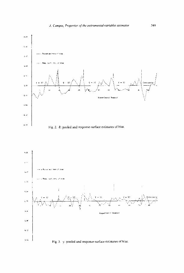
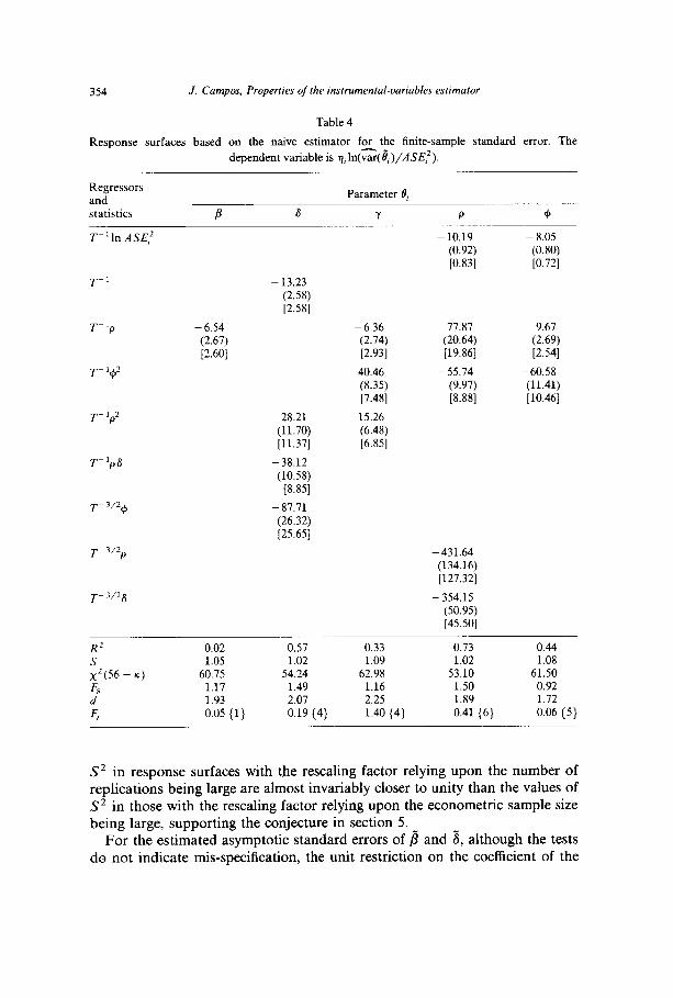
different from unity and so the unexplained variation is due to replacing the bias of 7 by its Monte Carlo estimator and not to mis-specification of the response surface. The biases are very small for 7, quite small for fi and 8, and somewhat larger for j?~ and 6; and, for all of them, the bias tends towards zero as the econometric sample size increases (see figs. l-5).

To evaluate the effects of autocorrelation and dynamics on the finite sample bias, let us consider the response surfaces based on the pooled estimates (see table 1). The estimated bias of fi is

&(/? - j3) = ,u:T-‘(2.25 + 0.17~ - l.OO@ (0.11) (0.08) (0.24) [O.lO] [0.07] [0.23]

- 1.35~~ + 1.33~8 - 0.676) (0.26) (0.21) (0.23) [0.22] [0.18] [0.18]

R2=0.78, S=1.16, Fs=1.31, d=2.22, F(r)=0.81, WI

x2(56 - K) = 67.75.

J. Cumpos, Properties of the insirumental-oariuhles estimator 349

Fig. 2. 6: pooled and response-surface estimates of bias.

Fig. 3. y: pooled and response-surface estimates of bias.

J. Cumpos, Properties of the insrrumentul-variables estimutor

Fig. 4. p: pooled and response-surface estimates of bias.

The effect of + on the bias of fi is positive for very small positive values (c$ < 0.17) and negative otherwise. The effect of p is positive for 0 < p < 8, and negative for p > 6 and for p -C 0. The effect of 6 is negative. However, the resultant bias of fi is always positive. From table 1, + positively biases 6 when C#I > 0 or + = - 0.5, having a negative effect otherwise. p positively biases 8 when p > 0 or p 5 -0.5. The effect of 6 is positive (negative) when both $J and p are negative (positive). For (p > 0 and p < 0, or + < 0 and p > 0, the effect of S is positive for values of 9 below - 2p, and negative otherwise. The resultant bias of 8 is generally negative. It is negative when + and p are both

non-positive. However, it is positive for large values of $I or p or both. It is certainly positive when C$ 2 0.2 and p 2 0.4. For $I > 0 and p < 0, the bias is positive for + and p large in absolute value (i.e., p -c -0.4 and + > 0.4). For C$ < 0 and p > 0, the bias of 8 is positive for p = 0.5 and + 5 0. The effects of Cp and p on the bias of 7 are positive (negative) if both parameters have the same (opposite) sign. The effect of 6 is positive for sample sizes below 53 and negative otherwise. For sample sizes below 77, the resultant bias of 7 is negative if + and p have opposite signs. For larger sample sizes or for + and p

having the same sign, the direction of the bias depends upon the values of the parameters. The effect of C#J on the bias of c is in the same (opposite) direction

J. Campos, Properties of the instrumental-unrrahles estlmutor 351

Fig. 5. +: pooled and response-surface estimates of bias.

as its sign, whenever T I 71 (T > 71). The effect of p is negative when p > 0, and so is the effect of 6 regardless of the values of the other parameters. When p -c 0, its effect on the bias of its own parameter is positive. The resultant bias of 7, is negative when $I < 0 and p > 0. It is also negative when + > 0 and

p 2 0.2. The bias can be positive when p < 0. The effect of p on the bias of 6 is in the same direction as its sign, as is the effect of $ for T 2 40. The effect of 6 is positive when p > 0. When p -c 0 the set of negative values of p for which 6 has a positive effect on the bias of 6, increases with the sample size. When p > 0, the resultant bias of 6 is positive for $B > 0, or $ < 0 and sample sizes below 60. When p < 0, the sign of the bias of 6 depends upon the sizes of all parameters, but the number of points (p, $I) for which the bias is positive increases with T.

The estimated standard errors of the coefficients in the response surface based on the pooled estimates of the biases are almost always smaller than those in comparable response surfaces based on the naive Monte Carlo estimates. The exception occurs when the response surface based on the pooled estimates includes extra regressors which are highly correlated with the common regressors. The average (and range) of the efficiency gains obtained by using control variates are given in table 2. An average efficiency gain of

352 J. Cumpos, Properties oj the instrumental-variuhles estimutor

Table 2

Average efficiency gains.”

Sample size T P 6 Y P 9

37 1.56 1.70 2.68 (1.06; 2.36) (1.02; 2.21) (1.77; 3.40)

57 2.08 2.35 3.82 (1.03; 2.92) (1.63; 4.61) (2.40; 6.75)

77 3.34 4.03 5.87 (1.55; 5.20) (1.70; 5.88) (2.16; 13.49)

97 4.33 4.02 6.78 (2.12; 7.48) (2.56; 6.27) (2.04; 13.55)

“The range of the efficiency gains is given in parentheses.

1.66 1.30 (0.65; 2.43) (0.85; 1.93)

2.37 1.81 (1.04; 3.48) (0.96; 3.21)

4.19 3.14 (1.74; 8.09) (1.77; 4.33)

4.40 3.88 (1.62; 6.63) (1.67; 5.75)

1.56 means that 56% more replications might be needed to obtain a naive estimate of the bias with the same standard error as the pooled estimate. At first sight, the efficiency gains may look small. However, the average comput- ing time is approximately 0.94 seconds per replication for T = 37 (most operations were done in double precision on a CDC computer), so that roughly 62 seconds of computer time would have been required to do those additional replications. As expected, the efficiency gains and saving in com- puter time are larger for larger econometric sample sizes: for instance, when T = 97 each replication takes on average 4.94 seconds of computer time but the efficiency gains are often three or larger. Table 3 gives the average (and range) of the estimated correlations between the naive and control-variate

estimates.

Table 3

Average estimated correlations between the naive and control-variate based estimates.a

Sample

size 7

37

57

77

97

P

0.66 (0.56; 0.78)

0.75 (0.57; 0.86)

0.84 (0.69; 0.90)

0.87 (0.77; 0.91)

6 Y P 9

0.68 0.79 0.70 0.58 (0.60; 0.81) (0.69; 0.85) (0.55; 0.79) (0.44; 0.72)

0.78 0.84 0.73 0.64 (0.72; 0.89) (0.77; 0.92) (0.53; 0.85) (0.38: 0.84)

0.86 0.90 0.88 0.84 (0.77; 0.91) (0.73; 0.96) (0.65; 0.94) (0.67; 0.88)

0.87 0.89 0.88 0.85 (0.81; 0.92) (0.73; 0.96) (0.77: 0.93) (0.73; 0.92)

A The range of the estimated correlations is given in parentheses.

J. Campos, Properties of the instrumentul-variables estmator 353

For the standard errors of fi, 8, 7, j? and 6, both response surfaces have the same form and their coefficients are within one standard error of each other. For 7, the variance of the disturbances is significantly different from unity in the second response surface. For /? and 6, the tests do not indicate mis-specifi- cation. For 8, fi and 6, a fair part of the variation in the estimated finite-sam- ple standard error is explained by finite-sample fluctuations. For p, R2 is low but the error variance is not significantly different from unity.

Because the response surface with the resealing factor TJ always gave an estimated error variance which was closer to unity than that obtained using q*, only the estimated variance functions based on TJ are discussed below (see table 4). As with the biases, the naive estimate of the finite-sample standard error and the response-surface estimate of the finite-sample standard error are quite close to each other and tend to the asymptotic value as the econometric sample size T increases. The estimated logarithm of the variance ratio of ,8 is

qrln[z( /?)/ASE2(fi)] = nr( - 6.54pTp1), [2.67] [2.60]

R2 = 0.02, S= 1.05, FR = 1.17, d= 1.93,

F( 7) = 0.05, x2(56 - K) = 60.75.

111

The absolute difference between the estimated finite-sample and asymptotic standard errors of p increases with p: for p > 0 (p < 0), the asymptotic standard error will be higher (lower) than the finite-sample one. From table 4, if p < 0, the difference between the two standard errors of 8 becomes more positive as p decreases and even more positive if cp < 0, cancelling in part the effect of T-‘. The resultant difference is negative for p > 0, for p 2 -0.3 and $I 2 -0.4, and for p < 0 and cp 2 0.2. The finite-sample standard error of 7 is higher than the asymptotic one if p < 0, regardless of the value of 9. For p

within [0,0.4], its effect compensates in’ part that of $. The difference is negative when p < 0.2 or p > - 0.2. Provided the asymptotic standard error is above one, the difference between the two standard errors of 5 is negative when p < 0, and for small sample sizes (T 5 50) when p > 0. Provided the asymptotic standard error of 6 is greater than unity, the difference between the two standard errors is negative when p -c 0, and when p > 0 for (p 2 0.3 or $I I -0.3. The term T-‘ln ASE2 has an indeterminate effect on the finite- sample standard errors of 6 and 4.

The two resealing factors for the naive Monte Carlo estimate of the bias (and of the standard error) did not give appreciably different results in terms of the coefficient estimates for the response surfaces. However, the values of

354 J. Campos, Properties of the instrumental-variables estimator

Table 4

Response surfaces based on the naive estimator fz the finite-sample standard error. The

dependent variable is n1 ln(var( 0,)/A SE:).

Regressors and statistics P

Parameter 0,

6 Y P +J

- 13.23 (2.58) [2.58]

- 6.54 - 6.36 (2.67) (2.74) [2.60] [2.93]

40.46 (8.35) [7.48]

28.21 15.26 (11.70) (6.48) [11.37] [6.85]

- 38.12 (10.58)

[8.85]

- 87.71 (26.32) [25.65]

- 10.19 (0.92) [0.83]

77.87 (20.64) [19.86]

- 55.74 (9.97) [8.88]

-431.64 (134.16) [127.32]

- 354.15 (50.95) [45.50]

- 8.05 (0.80) [0.72]

9.67 (2.69) [2.54]

- 60.58 (11.41) [10.46]

R2 0.02 0.57 0.33 0.73 0.44 s 1.05 1.02 1.09 1.02 1.08 x2(56 - K) 60.75 54.24 62.98 53.10 61.50 F, 1.17 1.49 1.16 1.50 0.92 d 1.93 2.07 2.25 1.89 1.72 F, 0.05 {l} 0.19 {4} 1.40 (4) 0.41 (6) 0.06 (5)

S* in response surfaces with the resealing factor relying upon the number of replications being large are almost invariably closer to unity than the values of S2 in those with the resealing factor relying upon the econometric sample size being large, supporting the conjecture in section 5.

For the estimated asymptotic standard errors of p and 8, although the tests do not indicate mis-specification, the unit restriction on the coefficient of the

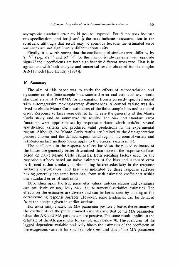
J. Cumpos, Properties of the instrumentul-vuriahles esttmator 355

asymptotic standard error could not be imposed. For y no tests indicate mis-specification; and for ,G and 6 the tests indicate autocorrelation in the residuals, although that result may be spurious because the estimated error variances are not significantly different from unity.

Finally, it is worth noting that the coefficients of similar terms differing by Tell2 (e.g., +T-’ and cpT_ 3/2 for the bias of +) always enter with opposite signs if their coefficients are both significantly different from zero. That is in agreement with both analytic and numerical results obtained for the simpler AR(l) model [see Hendry (1984)].

10. Summary

The aim of this paper was to study the effects of autocorrelation and dynamics on the finite-sample bias, standard error and estimated asymptotic standard error of IVARMA for an equation from a correctly specified model with autoregressive moving-average disturbances. A control variate was de- rived to obtain Monte Carlo estimators of the finite-sample bias and standard error. Response surfaces were defined to increase the generality of the Monte Carlo study and to summarize the results. The bias and standard error functions were approximated by response surfaces which satisfied several specification criteria and produced valid predictions in the experimental region. Although the Monte Carlo results are limited to the data-generation process chosen and the defined experimental region, the control-variate and response-surface methodologies apply to the general system in (1).

The coefficients in the response surfaces based on the pooled estimates of the biases are generally better determined than those in the response surfaces based on naive Monte Carlo estimates. Both resealing factors used for the response surfaces based on naive estimates of the bias and standard error performed rather similarly in eliminating heteroscedasticity in the response surface’s disturbances, and that was indicated by those response surfaces having generally the same functional form with estimated coefficients within one standard error of each other.

Depending upon the true parameter values, autocorrelation and dynamics can positively or negatively bias the instrumental-variables estimates. The effects on the estimates are diverse and can be better seen by looking at the corresponding response surfaces. However, some tendencies can be deduced from the analysis given in earlier sections.

For most sample sizes, the MA parameter positively biases the estimates of the coefficients of the predetermined variables and that of the MA parameter, when the AR and MA parameters are positive. The same result applies to the estimate of the AR parameter for sample sizes below 70. The coefficient of the lagged dependent variable positively biases the estimates of the coefficient of the exogenous variable for small sample sizes, and that of the MA parameter

356 J. Campos, Properties of the insirumental-uariahies estimator

when the AR parameter is positive, and negatively biases the estimates of the AR and endogenous variable coefficients. Its effect on the bias of its own estimate is also negative when the autocorrelation parameters are positive. If the AR parameter is negative, then it negatively biases the estimated coeffi- cients of the MA parameter. If the autocorrelation parameters have the same sign, then they positively bias the estimate of the coefficient of the exogenous variable and have a negative effect otherwise.

The bias of the estimate of the coefficient of the endogenous variable is positive. The estimate of the coefficient of the lagged endogenous variable is negatively biased when both the AR and the MA parameters are non-positive. However, the direction of the bias is reversed for most positive values of those parameters, and when the MA parameter is positive and the AR parameter is negative and both are large in absolute value. When the MA parameter is negative, large values of the AR parameter lead also to a positive bias. The estimate of the coefficient of the exogenous variable is biased downward when the MA and AR parameters have opposite signs and sample sizes are below 77. This bias is positive when both parameters have the same sign and are large in absolute value. The bias of the estimate of the AR parameter is negative for most positive values of that parameter. However, the estimate may become positively biased when the parameter is negative. The estimate of the MA parameter is biased upward for most sample sizes when the AR parameter is positive.

The difference between the finite-sample and the asymptotic standard errors (and between the estimated and the true asymptotic standard errors) may also be explained in terms of the autocorrelation and dynamics parameters. Some results on the direction of the error arising from using asymptotic standard errors are the following: The asymptotic standard error of the estimate of the coefficient of the endogenous variable overestimates (underestimates) the finite-sample standard error when the AR parameter is positive (negative). The finite-sample standard error of the estimate of the coefficient of the lagged dependent variable is generally overestimated. It is so when the AR parameter is positive, and when it is negative for large values (in absolute terms) of the AR and MA parameters and for most values of the MA parameter when this is positive. The standard error of the estimate of the coefficient of the exogenous variable is underestimated when the AR parameter is negative and overestimated when the MA parameter is small in absolute value. When the AR parameter is negative, the finite-sample standard error of its own estimate is overestimated by the asymptotic standard error, provided the latter is above unity. The same result is obtained for small sample sizes when the AR parameter is positive and the asymptotic standard error is above unity. Whenever the asymptotic standard error exceeds one, the finite-sample stan- dard error of the estimate of the MA parameter is overestimated if the AR parameter is negative and also when this is positive for large absolute values of

the MA parameter.

J. Campos, Properties of the Instrumental-ruriuhles estimator 357

The effect of individual parameters may compensate the effects of the others leading to small biases and/or small differences between finite-sample and asymptotic standard errors, making of IVARMA an estimator with sensible finite-sample properties for models similar to many found in applied econo- metrics.

Appendix A: A control variate for the bias and standard error of IVARMA

The control variate for the first two moments of IVARMA of the coeffi- cients in model (1) is derived assuming that the process generating (y,, zt) and the instruments Z* is ergodic. Letting f( ~9) = vet e’, the Taylor series expan- sion of (~A(8)/~~) about 0, gives

T~l(a24(e)/aeae~)l,++T1’2(8-e~)= -T-l/2(aqe)/ae)l,u,

6-w where 6++ lies on the line joining 8 and 0, and

(61A(6J)/~8)~e,,=2QG(I,@Z*‘)vecE’. 64.2)

Noting (A.l), (A.2) and the definition of ,X in section 2, define the CV estimator e* as

e*=eo-zQ+c+r1(I,8Z*‘)vecE’.

The first moment of the CV is

(A.31

E(O*) =8,-~Q+G’E[T-‘(l,c3Z*‘)vec~‘]. (A.4

Defining E, = (~,i . . . E,~)‘, the expectation on the right-hand side of (A-4) has

E( Tp ‘Z *‘E, )=E(T’~z;~,...T-~ ;,,.,,j’ r=l r=1

as its ith subvector, which is zero because zf*J and et, are uncorrelated. Hence that expectation is zero and so E(8*) = 0,.

The variance-covariance matrix of the CV is

E[(B*-8&j*-@,)‘] =BQ+G+E[(T-l~;Z*...Tpl~~Z*)’

x (T-%;z*...~-l &Z*)] G+Q+9. (AS)

358 J. Cumpos, Properties of the mstrumenrul-variables estimator

Apart from Tp2, the (i, j)th submatrix in the expectation in (A.5) is

E( Z*+;Z*) = E [i

; z;E;~.. . ; ZI*,*E., ’

t=1 t=l

i

T T

x c ZfrlE,, . . . c Zs*m*E,s s=l s=l 11 ; (A.6) and because the instruments Z* are assumed to be uncorrelated with current and future E’S and the latter are serially independent, the (h, I)th element of

that submatrix is

+ c ~E(z,*z.h)E(~,,) L<S

+ c ~E(zlC,z,*,~,.s)E(~u) f > s

T

= c E(z,*,z;)w,,= TE(z+$+ I=1

where o,, is the (i, j)th element of tie. Hence (A.6) is

E( Z*‘+Z*) = TE(z:z,+,,,

where z,! = (LX.. . z%, )‘. Thus the variance-covariance matrix of O* is

E[(B* - &)((I* -e,,)‘]

= T-‘_XQ+G+ [D @ plim( T-‘Z*‘Z*)] G’Q”z = T-‘lf.

To show that the CV and IVARMA are asymptotically equivalent, it will be proved that (8* - 8) = oP( T-lj2). Noting (A.1) (A.2) and that plim Z+’ = _X where .X++ = 2[T-l(a2d(e)/aeae’)l~++l-l,

8=e,-Z++QGT-‘(Z,@ZZ*‘)vecd. (47)

Subtracting (A.3) from (A.7),

j - e* = - [~++QG - 2Q+G+]T-l( z, c3 Z*')vec d. (A.8)

J. Cumpos, Properties of the instrumenfal-variables estimator 359

In (A.8), the term in square brackets is of o,(l), and the remaining term in that product is of OP(TW1/*) because T -‘/*(I,@Z*‘)vec~’ is O,(l). Hence (6-

0*) = o,(T-‘/*). However, note that if E’++ - 2 = Op(Tpl/*), Q - Q’ =

O,(T-‘I*) and G - G+ = O,(T-‘I*) [rather than o,(l), as assumed above], then we have the stronger result that (0 - (Z*) = O,(T-‘). This would also imply that V($li) would be the variance of a term of O,(T-‘) and V( q,,) would be the variance of a term of 0p(Tp3/2).

Appendix B: The asymptotic variance-covariance matrix of IVARMA for the first equation in the data-generation process

The AVM of IVARMA of the parameters of the first equation in the data-generation process (9) can be written as

wll [plim( T-‘( ae;/6’tZ)~,0Z*)plim( Z*‘Z*/T)-’

x plim( Tp’Z*‘( dq/dl?‘)~,o)] -l, W)

where ei is the T x 1 vector of disturbances in the first equation. The stochastic process generating the series (y,, z,) in (9) and (10) is ergodic [see Hannan (1970, p. 210)], so the probability limits in (B.l) can be written in terms of the population-data moments, the latter being calculated as functions of just the parameters of the model.

Before working out the probability limits in (B.l), consider the population- data moments as derived from the companion form f, = D*f,-i + ~7 of the

data-generation process, where f,’ = ( y;, J$_ 1, z;), 07’ = ((B; ‘( E, + SE!_ 1 -

C,u,))‘,O’, u;) and D* is a partitioned matrix whose elements DG are zero except for DTl = -B; ‘( B, - RB,), OF2 = B; ‘RB,, 05 = -B, ‘( C,A - RC,),

0; = I, and DT3 = A. The moment matrices of o,* with itself and its lagged values are E(w$$+‘) = r,, E(o$,*l,) = r2 and E(w:w:‘) = 0 for all t and s satisfying ]t - S] > 1. In those matrices, all elements are zero, except for

E( UT&,‘) = B, ‘( f12, + SO,S’ + C,s2,C;)( B, l)‘, E( o;&‘) = - B, ‘C,$,,, E(w:,w$;) = a, and E(~T,uT,‘,_~) = B;‘Sti,(B;‘)‘.

The contemporaneous population-data moment matrix M(0) = E( f,f,‘) can be obtained from the expression vet M(0) = (I - D* ~8 D*) - ’ vec( D*r; +

r,D*’ + r,). The one-period lag population-data moment matrix is M(1) = E(f,f,Yi) = D*M(O) + r,, and it can be shown by induction that

M(a)=(D*)“-‘M(1) forall ~21. (B.2)

Also M(a) = M’( - a) because of stationarity. Let us assume that the instrumental variables z: are the predetermined

variables in the system and all those variables lagged up to given orders, less

any redundant variables. That is, z: = (y,,,_,,. .., .Y~,+~,, Y~,~_~, . . . . y2,1--J2,

Zi,, . . ., Z1,,-G1,. . ., Z4,?. . .? Z4,t-G, )‘, z*=(zf,..., I;)’ and the number of

360 J. Campos, Properties of the insirumental-variables estimator

instrumental variables is m * = [.I1 +J2 + c~=,(G, + l)]. The first row in piim[T-‘( Jei/H)Z*] is plim[T-‘( ae;/@)Z*]. The first (Jr + J2) elements of that vector are of the form plim[T-lC~=,( aq,/6’/3)y,,t_i8] (j, = 1,. . . , J,; i = 1,2), and the remaining Cy=,(G, + 1) elements are of the form

plim[T-‘C~=,(a&,JaP)z,,l~g,] (g,=O ,..., G,; i=l,..., 4). From the stationarity and ergodicity of the variables in (9) and (lo), an

element corresponding to the instrument yr,+,, is

T-’ i (~~,/@)YI,,-~~ r=1 1

= E(Y,,Y~,,-~,) - @(Y,,,-,Y,,,-,,I + f (-~)kE(Y2.r-kyl,r~i,)

k=l

-P : (-~)kE(~~,~-k-lL.l,r~h)

k=l

=m,*(-j,)-pm,,(l-j,)+ f (-@4”J%(~-~,)

k=l

where mh,( a) is the (h, j)th element of the data moment matrix M(a). The algebra is similar for the elements corresponding to the instruments y2,+,,

and zi ,_-g. 1 I Using (B.2) and (C.l), those elements simplify to

dim [ T-’ JZ (~+‘JP)~i,t-j, =Pi,(ji) - PPiz(ji- 113

I=1 1 j, = 1 ,..., Jl, i= 1,2, (B.3) and

plim 1 T-’ i (~s,,/W)z,,,-, 1 =Pi+d,*(gi) - PPt+4,2(gr- l>,

t=1

g,=O,...,G,, i = 1,2,3,4, (B.4)

where ~~,(a) is the (h, j)th element of the matrix P(a) (see appendix C).

J. Cumpos, Properties of the instrumental-variables estimam 361

The second, third and fourth row in plim[T-‘( Je;/80)Z*] can be obtained in a similar way. Their elements are

Him [ T-’ i ta%/J~)Y;,t-, =Pil(jlel) -PPil(jl-2)t

t=1 1

j;= l,..., 4, i=1,2, (B-5)

plim T-l t=1 I =P,+‘l,dgi - 1) - PPi+&i - 2)?

g, = 0 >‘.., G,, i= 1,2,3,4, (B.6)

plim i

T-’ 5 (a&l,/aY)yj,,-, ‘PiS(ii) - PPiS(jr- ‘15

t=1 1 j;= l,..., 4, i=1,2. (B.7)

and

slim T-’ 5 taE~JaY)zi,~-~, =Pt+4,5tgO - PPi+d,S(gi- ‘>,

t=1 1 g,=O ,..., G,, i=1,2,3,4, (B.8)

plim T-’ i (aElJ@)x,,-i, t=1 1

j;= l,..., J., i=1,2, (B.9)

dim T-’ f (adJp)zi,t-g, t=1 1

g, = 0 ,..., Gi, i=1,2,3,4.

(B.lO)

J.E -~C

362 J. Campos, Properiies of the insirumenral-variables estimator

Using (C.3) plim[T-‘(8&;/6’$)Z*], the fifth row of plim(T-‘(a&‘aO)Z*), has elements

+Yws(“h - 1) + PPW;,(i - 1) - PW,,(j,>> (B.11)

and

j,=l,..., 4, i=1,2,

= W~+4,1(gr) - C6 + P)w,+4,1(gi- ‘) + GPw,+4,1(g,-2)

-YW,+‘&J + YW+&, - 1)

+PPwi+4,2(gr- ‘1 - Pwi+4,2(gi), (B.12)

g,=O ,..., G,, i=1,2,3,4,

where ~,,~(a) is the (h, j)th element of the matrix W(a) (see appendix C). From (B.3) to (B.12) the matrix plim[T-‘( ae;/aO)Z*] can be constructed.

The matrix plim(T-‘Z*‘Z*) can be partitioned to have M,, as its (i, j)th

element, where Ml, is the population variance-covariance matrix of the

instruments (yl, 1_ i, . .9 Yl, l-J1’ Y,, f- 17. . .? Y2, IFJ,, zw . . . 9 z~,~-~,), Ml2 is the cowiance matrix of (~l,1-1,...,~l,t-J,,~2,1-1,...,~2.,~J,,~lt,...,~1,,~GI) with (z,~,. . ., z;,,-~,) (i = 2,3,4), and M22 is the variance-covariance matrix

Of (‘it,...? ‘,,r-G ) (i = 2,3,4). Using the M;,‘s to calculate plim( T-‘Z*‘Z*), the AVM can be’obtained from (B.l).

Appendix C: The derivation of P(a) and W(a)

In the discussion below, it is assumed that ]+I < 1.

C.l. Derivation of P(a)

Let

P(a)=M(-a)+ f (-$)kM(k-a). k=l

J. Cumpos, Properties of the instrumental-vurrahles estimator 363

It can be shown that

P(a)=M(-a)+ f (-l#l)kM(k-a) k=l

+ (-~)“+‘(z+~D)-‘M(1), _ a2 1,

=M(O) + (-+)(z++D)-‘M(l), a=o, (c.1)

= (z+c#lD)-‘M(-a), a < 0.

The proof is given for a 2 1 only, since the algebra is similar for a 6 0.

u+l

P(a) =M(-a) + c (-$)kM(k-a) k=l

+ E (-c$)%(k-a). k=o+2

(c.2)

Because M(s) = D”-‘M(1) for all s 2 1, the third term on the right-hand side of (C.2) is

F (-c#M(k - a) = 5 ( -,)h+“+‘DhM(l) h=o+2 h=l

The last equality sign follows from solving for the matrix of coefficients of A ( $I), where

H(+)=Z+ f (-I$)~D~, h=l

and

Because A(+)H(+) = I, then A, = I, A, = D and A, = 0 for all s 2 2, so A(+) = (I + +D) and H($J) = (I+ +D)-‘. Hence (C.2) is

P(a)=M(-a)+ i (-$$%(k-a)+(-~)U+‘(Z+~D)-‘M(l). k=l

364 J. Campos, Properties of the instrumental-variables estimator

For a > 1, the matrix P(a) can be calculated using the following recursive formulae:

P,* = (-@34(O) and Ps*=(-+)sM(s-a)+Ps~,, a>szl,

where

P,*= 2 (-+)kM(k-u), k=s

and

P(a)=M(-n)+P:+(-+)a+l(l++D)-lM(l).

C.2. Derivation of W(u)

Let

w(u) = M(1 - u) + f k( -+)k-lM(k - u). k=2

It can be shown that

W(u)=M(l-a)+ 2 k(-+)k-1M(k-u)+(-4y k=2

x(I+c$D)-‘[(I++D)-‘+ul]M(l), ~22,

= M(0) -t- (-$)(I+ +D)-'M(1)

+ (-d(Z+W-2~M(l), u=l,

= (Z++D)-‘M(1 -a), a s 0. (C.3)

The proof is given for a 2 2,

w(u) = M(1 - u) + i k(-+yM(k - u) k=2

+ F k(-l#l)k-‘M(k-u). k=u+l

(C.4)

J. Campos, Properties of the inslrumental-variables estimator 365

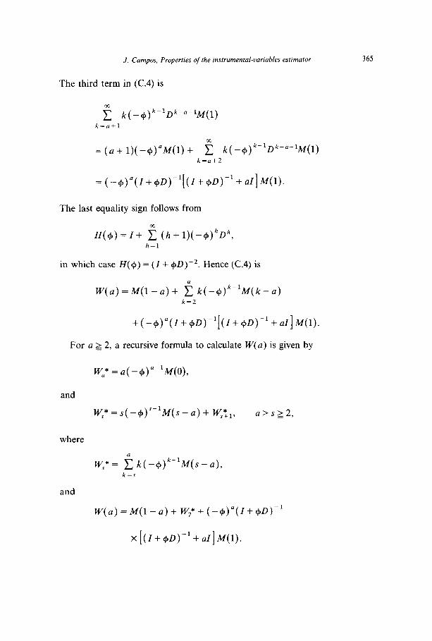
The third term in (C.4) is

E k(-$plDk-~--lM(l) k=otl

= (a + l)( -$)94(l) + E k( -Q)k-1Dk-o-94(1) k=a+2

= (-~)“(z+~D)-‘[(z+~D)-‘+al]~(1).

The last equality sign follows from

zY(c#l)=z+ f (h-tl)(-&DA, h=l

in which case II(+) = (I + I$D)-~. Hence (C.4) is

W(a)=M(l-a)+ i k(-Qp’M(k-a) k=2

+(-+)“(I+@-‘[(I+@)-‘+az]M(l).

For a 2 2, a recursive formula to calculate W(a) is given by

w,* = u( -c$)“-‘M(O),

and

w,*=s(-+)“-‘M(s-a)+ ws*+l, _ U>Sl2,

where

w,* = f k( -~)k-lM(s- a), k=s

and

W(u)=M(l-a)+ W;t+(-$)“(z+@-’

x[(z+l#Jo)-‘+uz]M(l).

366 J. Cumpos, Properties of the rnstrumentul-vurtubles esttmutor

Aneuryn-Evans. G. and A. Deaton, 1980, Testing linear versus logarithmic regression models. Review of Economic Studies 47, 275-291.

Bowden. R.J. and D.A. Turkington, 1984, Instrumental variables (Cambridge University Press, Cambridge).

Box. G.E.P. and M.E. Muller, 1958, A note on the generation of random normal deviates, Annals of Mathematical Statistics 29, 610-611.

Campos, J., 1982, Instrumental variables estimation of dynamic economic systems with autocorre- lated errors, Ph.D. thesis (London School of Economics, London).

Campos, J., 1986, Instrumental variables estimation of dynamic simultaneous systems with ARMA errors, Review of Economic Studies 53. 125-138.

Chow, G.C., 1960, Tests of equality between sets of coefficients in two linear regressions. Econometrica 28, 591-605.

Cramer, H., 1946, Mathematical methods of statistics (Princeton University Press, Princeton, NJ), Deistler, M. and J. Schrader, 1979, Linear models with autocorrelated errors: Structural identif-

ability in the absence of minimality assumptions, Econometrica 47, 4955504. Durbin, J. and G.S. Watson, 1950. Testing for serial correlation in least squares regression I,

Biometrika 37, 409-428. Durbin, J. and G.S. Watson, 1951, Testing for serial correlation in least squares regression II,

Biometrika 38, 159-178. Hannan, E.J., 1970, Multiple time series (Wiley, New York). Hendry, D.F., 1984, Monte Carlo experimentation in econometrics, Ch. 16 in: Z. Griliches and

M.D. Intriligator, eds., Handbook of econometrics. Vol. II (North-Holland, Amsterdam). Hendry, D.F. and R.W. Harrison, 1974, Monte Carlo methodology and the small sample

behaviour of ordinary and two-stage least squares, Journal of Econometrics 2, 151-174. Hendry, D.F. and F. Srba, 1977, The properties of autoregressive instrumental variables estima-

tors in dynamic systems, Econometrica 45, 9699990. Mann, H.B. and A. Wald, 1943. On stochastic limit and order relationships, Annals of Mathemati-

cal Statistics 14, 217-226. Mizon, G.E. and D.F. Hendry, 1980, An empirical application and Monte Carlo analysis of tests

of dynamic specification, Review of Economic Studies 47, 21-45. Nagar, A.L., 1959, The bias and moment matrix of the general k-class estimators of the

parameters in simultaneous equations, Econometrica 27, 575-595. Phillips, P.C.B., 1980, Finite sample theory and the distribution of alternative estimators of the

marginal propensity to consume, Review of Economic Studies 47, 183-224. Sargan, J.D., 1958, The estimation of economic relationships using instrumental variables,

Econometrica 26, 393-415. Sargan, J.D., 1959, The estimation of relationships with autocorrelated residuals by the use of

instrumental variables, Journal of the Royal Statistical Society B 21, 91-105. Sargan, J.D., 1976, Econometric estimators and the Edgeworth approximation, Econometrica 44,

421-448, and 1977, Erratum, Econometrica 45, 272. Theil, H., 1971, Principles of econometrics (Wiley, New York). White, H., 1980a, Using least squares to approximate unknown regression functions, International

Economic Review 21,149-170. White, H., 1980b, A heteroskedasticity-consistent covariance matrix estimator and a direct test for

heteroskedasticity, Econometrica 48, 817-838.