finite size e ects in integrable qfts zolt an bajnok
TRANSCRIPT

Integrability in Gauge and String Theory, 29 June - 3 July 2009, Potsdam, Germany
Finite size effects in integrable QFTsZoltan Bajnok,
Hungarian Academy of Sciences, Eotvos University, Budapest
AdS←→integrable model←→CFT
1

Integrability in Gauge and String Theory, 29 June - 3 July 2009, Potsdam, Germany
Finite size effects in integrable QFTsZoltan Bajnok,
Hungarian Academy of Sciences, Eotvos University, Budapest
AdS←→integrable model←→CFT

Integrability in Gauge and String Theory, 29 June - 3 July 2009, Potsdam, Germany
Finite size effects in integrable QFTsZoltan Bajnok,
Hungarian Academy of Sciences, Eotvos University, Budapest
AdS←→integrable model←→CFT
g
Classical string theory
Semiclassical string theory
J
1 loop perturbative gauge theory
+ string loop corrections
Nonperturbative gauge theory
Quantum String theory
S −
mat
rix
+ gauge loop corrections
Asy
mpt
otic
Bet
he A
nsat
z
Wra
ppin
g/Lu
sche
r co
rrec
tion
Finite J (volume) integrable models: (Lee-Yang, sinh-Gordon, sine-Gordon)←→AdS/CFT

Motivation: AdS/CFT
2

Motivation: AdS/CFT
g
J

Motivation: AdS/CFT
g
Classical string theory
J

Motivation: AdS/CFT
g
Classical string theory
Semiclassical string theory
J

Motivation: AdS/CFT
g
Classical string theory
Semiclassical string theory
J
+ string loop corrections
Quantum String theory

Motivation: AdS/CFT
g
Classical string theory
Semiclassical string theory
J
1 loop perturbative gauge theory
+ string loop corrections
Quantum String theory

Motivation: AdS/CFT
g
Classical string theory
Semiclassical string theory
J
1 loop perturbative gauge theory
+ string loop corrections
Nonperturbative gauge theory
Quantum String theory
+ gauge loop corrections

Motivation: AdS/CFT
g
Classical string theory
Semiclassical string theory
J
1 loop perturbative gauge theory
+ string loop corrections
Nonperturbative gauge theory
Quantum String theory
S −
mat
rix
+ gauge loop corrections

Motivation: AdS/CFT
g
Classical string theory
Semiclassical string theory
J
1 loop perturbative gauge theory
+ string loop corrections
Nonperturbative gauge theory
Quantum String theory
S −
mat
rix
+ gauge loop corrections
Asy
mpt
otic
Bet
he A
nsat
z

Motivation: AdS/CFT
g
Classical string theory
Semiclassical string theory
J
1 loop perturbative gauge theory
+ string loop corrections
Nonperturbative gauge theory
Quantum String theory
S −
mat
rix
+ gauge loop corrections
Asy
mpt
otic
Bet
he A
nsat
z
Wra
ppin
g/Lu
sche
r co
rrec
tion
Need finite J (volume) solution of the spectral problem

Plan of talk
3

Plan of talk
Classical integrable models: sine-Gordon theory0
V
2 πβ φ
AdS5
S5

Plan of talk
Classical integrable models: sine-Gordon theory0
V
2 πβ φ
AdS5
S5
Quantization of integrable models: sine-Gordon model: PCFT

Plan of talk
Classical integrable models: sine-Gordon theory0
V
2 πβ φ
AdS5
S5
Quantization of integrable models: sine-Gordon model: PCFT
Bootstrap approach to quantum integrable models: S=scalar.matrix p p
1
21
2
p
3
3
p p p
p
1
1
2
p
3
3
p p p
p2

Plan of talk
Classical integrable models: sine-Gordon theory0
V
2 πβ φ
AdS5
S5
Quantization of integrable models: sine-Gordon model: PCFT
Bootstrap approach to quantum integrable models: S=scalar.matrix p p
1
21
2
p
3
3
p p p
p
1
1
2
p
3
3
p p p
p2
Lee-Yang, sinh-Gordon, sine-Gordon↔ AdS σmodel+−
Bn
B
B B
B
Finite volume: Asymptotic Bethe Ansatz:
p
2p
n
p1
Luscher correction
Exact: groundstate TBA,
L
Re−H(R) L
L
e−H(L)R
R
Excited TBA, Y-system, NLIE...
p
p+1
Conclusion

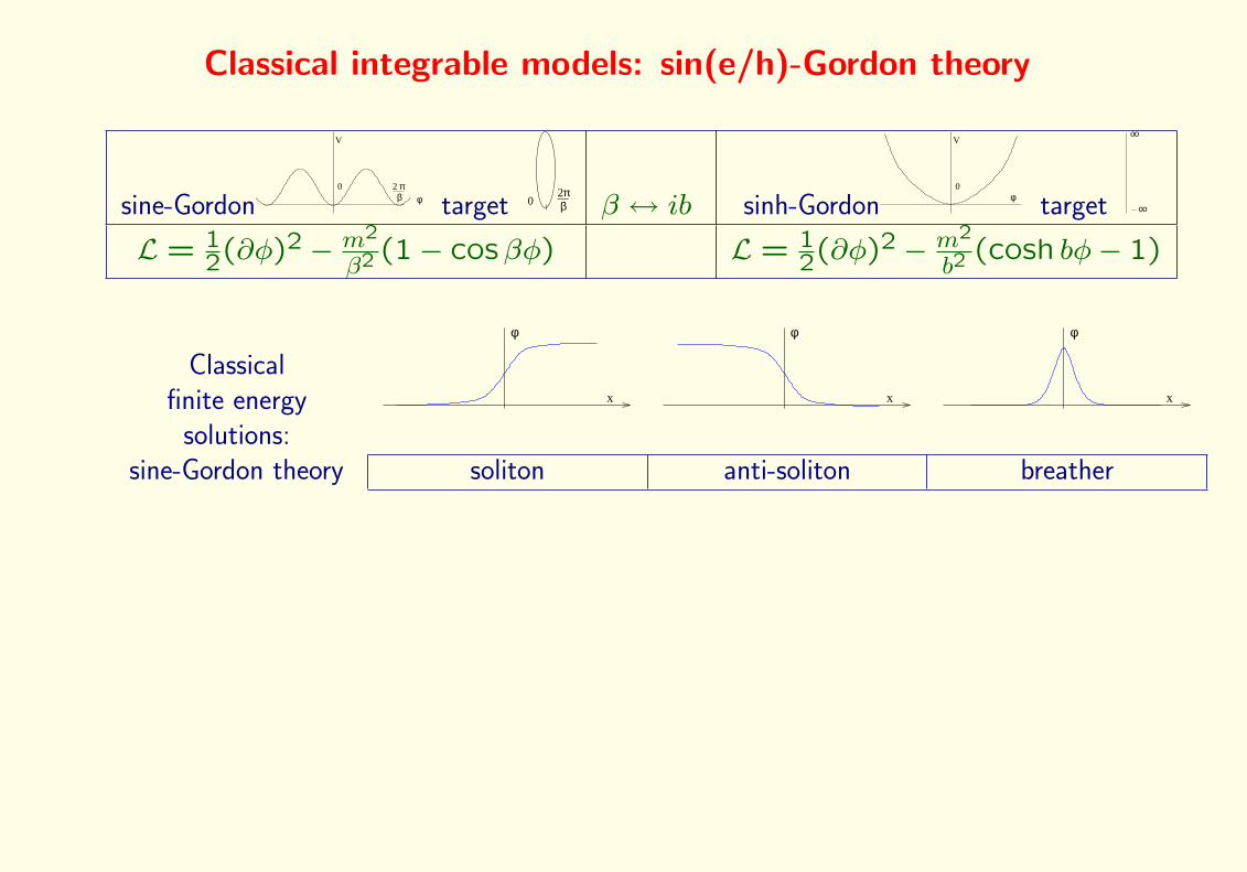
Classical integrable models: sin(e/h)-Gordon theory
sine-Gordon0
V
2 πβ φ target 0
2πβ β ↔ ib sinh-Gordon
0
V
φ target οο
οο
L = 12(∂φ)2 − m2
β2 (1− cosβφ) L = 12(∂φ)2 − m2
b2(cosh bφ− 1)
4
Classical integrable models: sin(e/h)-Gordon theory
sine-Gordon0
V
2 πβ φ target 0
2πβ β ↔ ib sinh-Gordon
0
V
φ target οο
οο
L = 12(∂φ)2 − m2
β2 (1− cosβφ) L = 12(∂φ)2 − m2
b2(cosh bφ− 1)
Classicalfinite energy
solutions:
x
φ
x
φ
x
φ
sine-Gordon theory soliton anti-soliton breather

Classical integrable models: sin(e/h)-Gordon theory
sine-Gordon0
V
2 πβ φ target 0
2πβ β ↔ ib sinh-Gordon
0
V
φ target οο
οο
L = 12(∂φ)2 − m2
β2 (1− cosβφ) L = 12(∂φ)2 − m2
b2(cosh bφ− 1)
Classicalfinite energy
solutions:
x
φ
x
φ
x
φ
sine-Gordon theory soliton anti-soliton breather
Integrability: ∂xAt − ∂tAx + [Ax, At] = 0↔ T (µ) = P exp∮A(x)νdxν
Ax(µ) = i2
(2µ β∂+ϕ
−β∂+ϕ −2µ
)At(µ) = 1
4iµ
(cosβϕ −i sinβϕi sinβϕ − cosβϕ
)T
gTg−1
conserved Q±1[ϕ] = E[ϕ]± P [ϕ] =∫ {1
2(∂±ϕ)2 + m2
β2 (1− cosβϕ)}dx
charges: Q±3[ϕ] =∫ {1
2(∂2±ϕ)2 − 1
8(∂±ϕ)4 + m2
β2 (∂±ϕ)2(1− cosβϕ)}

Classical integrable models: sin(e/h)-Gordon theory
sine-Gordon0
V
2 πβ φ target 0
2πβ β ↔ ib sinh-Gordon
0
V
φ target οο
οο
L = 12(∂φ)2 − m2
β2 (1− cosβφ) L = 12(∂φ)2 − m2
b2(cosh bφ− 1)
Classicalfinite energy
solutions:
x
φ
x
φ
x
φ
sine-Gordon theory soliton anti-soliton breather
Integrability: ∂xAt − ∂tAx + [Ax, At] = 0↔ T (µ) = P exp∮A(x)νdxν
Ax(µ) = i2
(2µ β∂+ϕ
−β∂+ϕ −2µ
)At(µ) = 1
4iµ
(cosβϕ −i sinβϕi sinβϕ − cosβϕ
)T
gTg−1
Classical factorized scattering: time delays sums up ∆T1(v1, v2, . . . , vn) =∑i∆T1(v1, vi)
Τ vvv1 2 n> > ... >
.
v Τ1
v <2< ... <vn

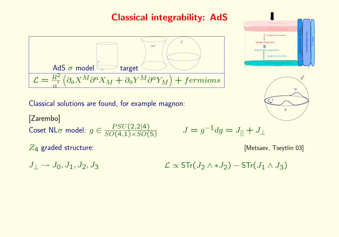
Classical integrability: AdSg
Classical string theory
Semiclassical string theory
J
1 loop perturbative gauge theory
+ string loop corrections
Nonperturbative gauge theory
Quantum String theory
S −
mat
rix
+ gauge loop corrections
Asy
mpt
otic
Bet
he A
nsat
z
Wra
ppin
g/Lu
sche
r co
rrec
tion
AdS σ modelτ
σ target
AdS5
S5
L = R2
α′(∂aXM∂aXM + ∂aYM∂aYM
)+ fermions
5

Classical integrability: AdSg
Classical string theory
Semiclassical string theory
J
1 loop perturbative gauge theory
+ string loop corrections
Nonperturbative gauge theory
Quantum String theory
S −
mat
rix
+ gauge loop corrections
Asy
mpt
otic
Bet
he A
nsat
z
Wra
ppin
g/Lu
sche
r co
rrec
tion
AdS σ modelτ
σ target
AdS5
S5
L = R2
α′(∂aXM∂aXM + ∂aYM∂aYM
)+ fermions
Classical solutions are found, for example magnon:
[Zarembo]
S5
p
−p
J
Coset NLσ model: g ∈ PSU(2,2|4)SO(4,1)×SO(5) J = g−1dg = J||+ J⊥
Z4 graded structure: [Metsaev, Tseytlin 03]
J⊥ → J0, J1, J2, J3 L ∝ STr(J2 ∧ ∗J2)− STr(J1 ∧ J3)

Classical integrability: AdSg
Classical string theory
Semiclassical string theory
J
1 loop perturbative gauge theory
+ string loop corrections
Nonperturbative gauge theory
Quantum String theory
S −
mat
rix
+ gauge loop corrections
Asy
mpt
otic
Bet
he A
nsat
z
Wra
ppin
g/Lu
sche
r co
rrec
tion
AdS σ modelτ
σ target
AdS5
S5
L = R2
α′(∂aXM∂aXM + ∂aYM∂aYM
)+ fermions
Classical solutions are found, for example magnon:
[Zarembo]
S5
p
−p
J
Coset NLσ model: g ∈ PSU(2,2|4)SO(4,1)×SO(5) J = g−1dg = J||+ J⊥
Z4 graded structure: [Metsaev, Tseytlin 03]
J⊥ → J0, J1, J2, J3L ∝ STr(J2 ∧ ∗J2)− STr(J1 ∧ J3)
Integrability from flat connection: dA−A ∧A = 0
A(µ) = J0 + µ−1J1 + (µ2 + µ−2)J2/2 + (µ2 + µ−2)J2/2 + µJ3
Conserved charges from the trace of the monodromy matrix
T (µ) = P exp∮A(x)µdxµ
T
gTg−1
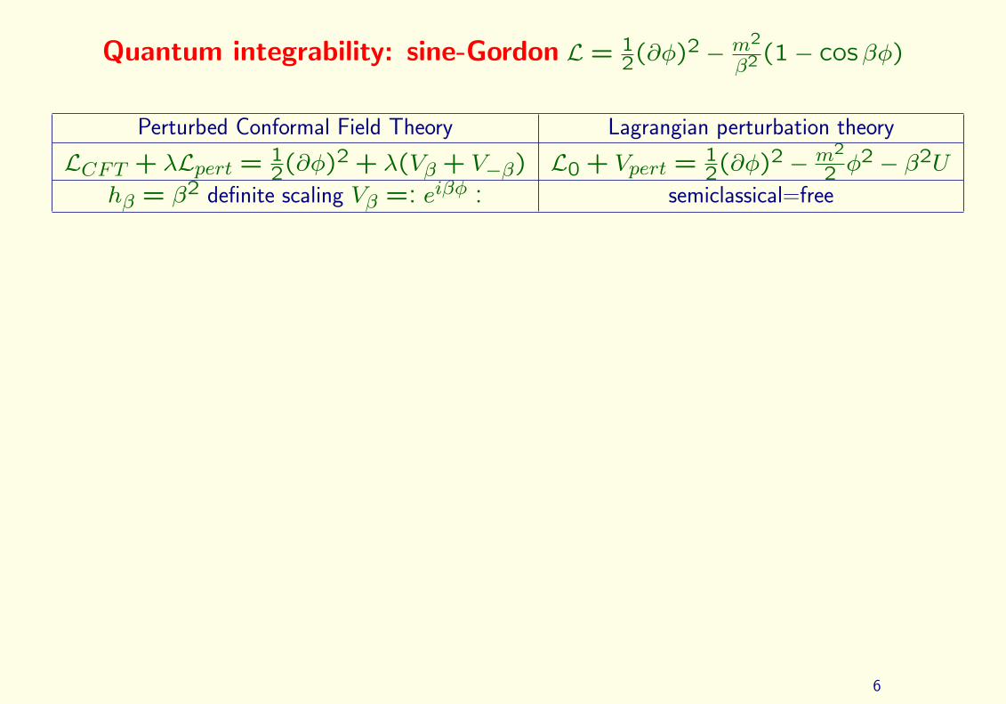
Quantum integrability: sine-Gordon L = 12(∂φ)2 − m2
β2 (1− cosβφ)
Perturbed Conformal Field Theory Lagrangian perturbation theory
LCFT + λLpert = 12(∂φ)2 + λ(Vβ + V−β) L0 + Vpert = 1
2(∂φ)2 − m2
2 φ2 − β2U
hβ = β2 definite scaling Vβ =: eiβφ : semiclassical=free
6

Quantum integrability: sine-Gordon L = 12(∂φ)2 − m2
β2 (1− cosβφ)
Perturbed Conformal Field Theory Lagrangian perturbation theory
LCFT + λLpert = 12(∂φ)2 + λ(Vβ + V−β) L0 + Vpert = 1
2(∂φ)2 − m2
2 φ2 − β2U
hβ = β2 definite scaling Vβ =: eiβφ : semiclassical=free
Quantum conservation laws [Zamolodchikov]
∂−Λ4 = 0→ ∂−Λ4 = λ∂+Θ2[λ] = 2− hβ, [Λ4] = 4,
Nonlocal symmetries Uq(sl2)
Correlators=∑loops Feynmandiagrams
Asymptotic states E(p) =√p2 +m2
S-matrix↔correlators LSZunitarity, crossing symmetry, analyticity
Bootstrap scheme
Quantum integrability: AdS no proof !
Perturbative integrability see [Zarembo]s talk and also
[Lipatov, Zarembo, Minahan, Staudacher, Beisert, Kristjansen, Bena, Polchinski, Roiban]

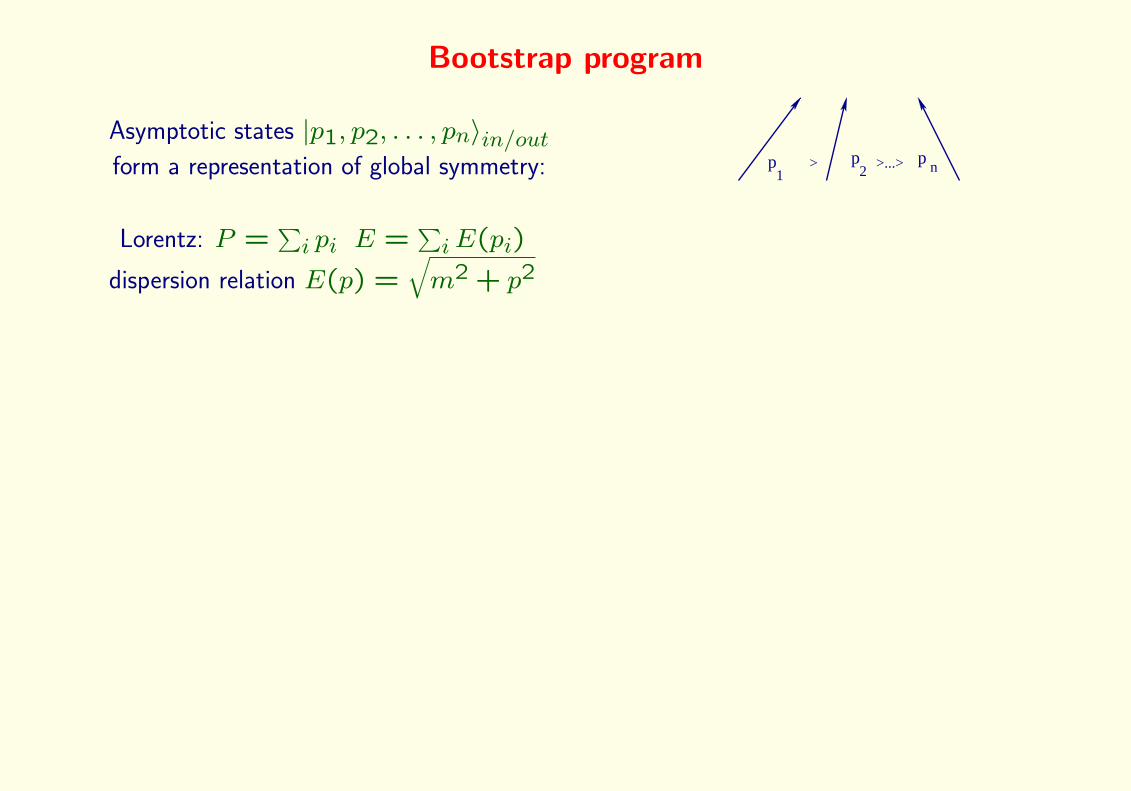
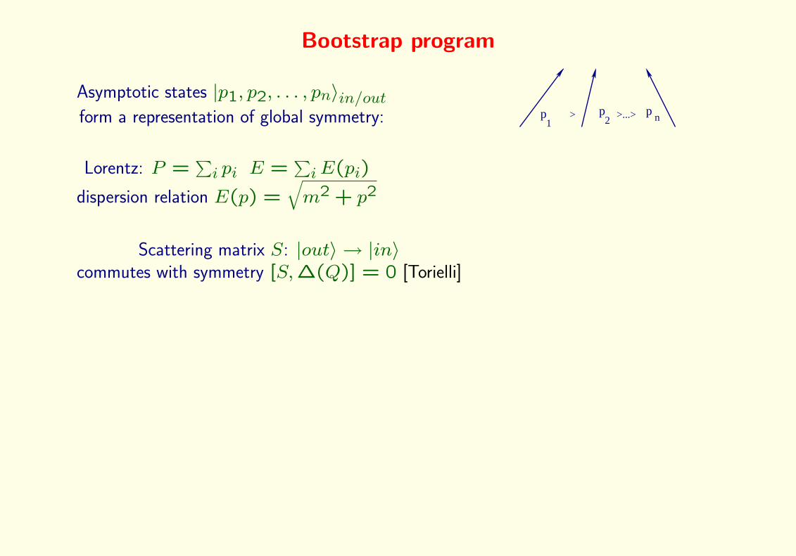
Bootstrap program
Asymptotic states |p1, p2, . . . , pn〉in/outform a representation of global symmetry: p p
21> >...> p
n
7
Bootstrap program
Asymptotic states |p1, p2, . . . , pn〉in/outform a representation of global symmetry: p p
21> >...> p
n
Lorentz: P =∑i pi E =
∑iE(pi)
dispersion relation E(p) =√m2 + p2

Bootstrap program
Asymptotic states |p1, p2, . . . , pn〉in/outform a representation of global symmetry: p p
21> >...> p
n
Lorentz: P =∑i pi E =
∑iE(pi)
dispersion relation E(p) =√m2 + p2
p p1
pn2
∆(Q)
Bootstrap program
Asymptotic states |p1, p2, . . . , pn〉in/outform a representation of global symmetry: p p
21> >...> p
n
Lorentz: P =∑i pi E =
∑iE(pi)
dispersion relation E(p) =√m2 + p2
Scattering matrix S: |out〉 → |in〉commutes with symmetry [S,∆(Q)] = 0 [Torielli]

Bootstrap program
Asymptotic states |p1, p2, . . . , pn〉in/outform a representation of global symmetry: p p
21> >...> p
n
Lorentz: P =∑i pi E =
∑iE(pi)
dispersion relation E(p) =√m2 + p2
Scattering matrix S: |out〉 → |in〉commutes with symmetry [S,∆(Q)] = 0 [Torielli]
p p
S−matrix
1
21> >...>
p’p’m
< p’2
<...<
pn
(Q)∆
(Q)∆
Higher spin concerved charge
factorization + Yang-Baxter equation
S123 = S23S13S12 = S12S13S23
p p
1
21
2
p
3
3
p p p
p
1
1
2
p
3
3
p p p
p2
S-matrix = scalar . Matrix

Bootstrap program
Asymptotic states |p1, p2, . . . , pn〉in/outform a representation of global symmetry:
p p21
> >...> pn
Lorentz: P =∑i pi E =
∑iE(pi)
dispersion relation E(p) =√m2 + p2
Scattering matrix S: |out〉 → |in〉commutes with symmetry [S,∆(Q)] = 0 [Torielli]
p p
S−matrix
1
21> >...>
p’p’m
< p’2
<...<
pn
(Q)∆
(Q)∆
Higher spin concerved charge
factorization + Yang-Baxter equation
S123 = S23S13S12 = S12S13S23p p
1
21
2
p
3
3
p p p
p
1
1
2
p
3
3
p p p
p2
S-matrix = scalar . Matrix
Unitarity S12S21 = Id
Crossing symmetry S12 = S21Maximal analyticity: all poles have physical origin→ boundstates, anomalous thresholds

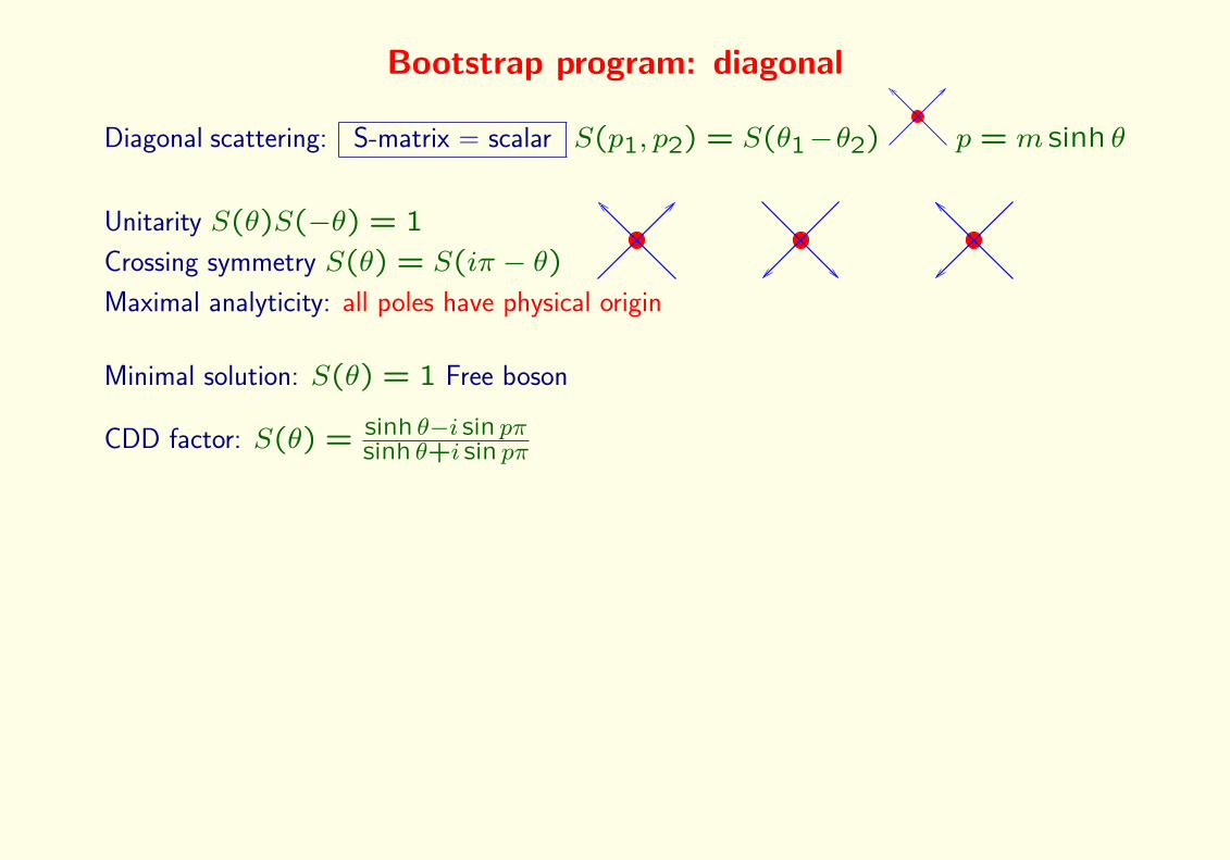
Bootstrap program: diagonal
Diagonal scattering: S-matrix = scalar S(p1, p2) = S(θ1−θ2) p = m sinh θ
8

Bootstrap program: diagonal
Diagonal scattering: S-matrix = scalar S(p1, p2) = S(θ1−θ2) p = m sinh θ
Unitarity S(θ)S(−θ) = 1
Crossing symmetry S(θ) = S(iπ − θ)
Maximal analyticity: all poles have physical origin

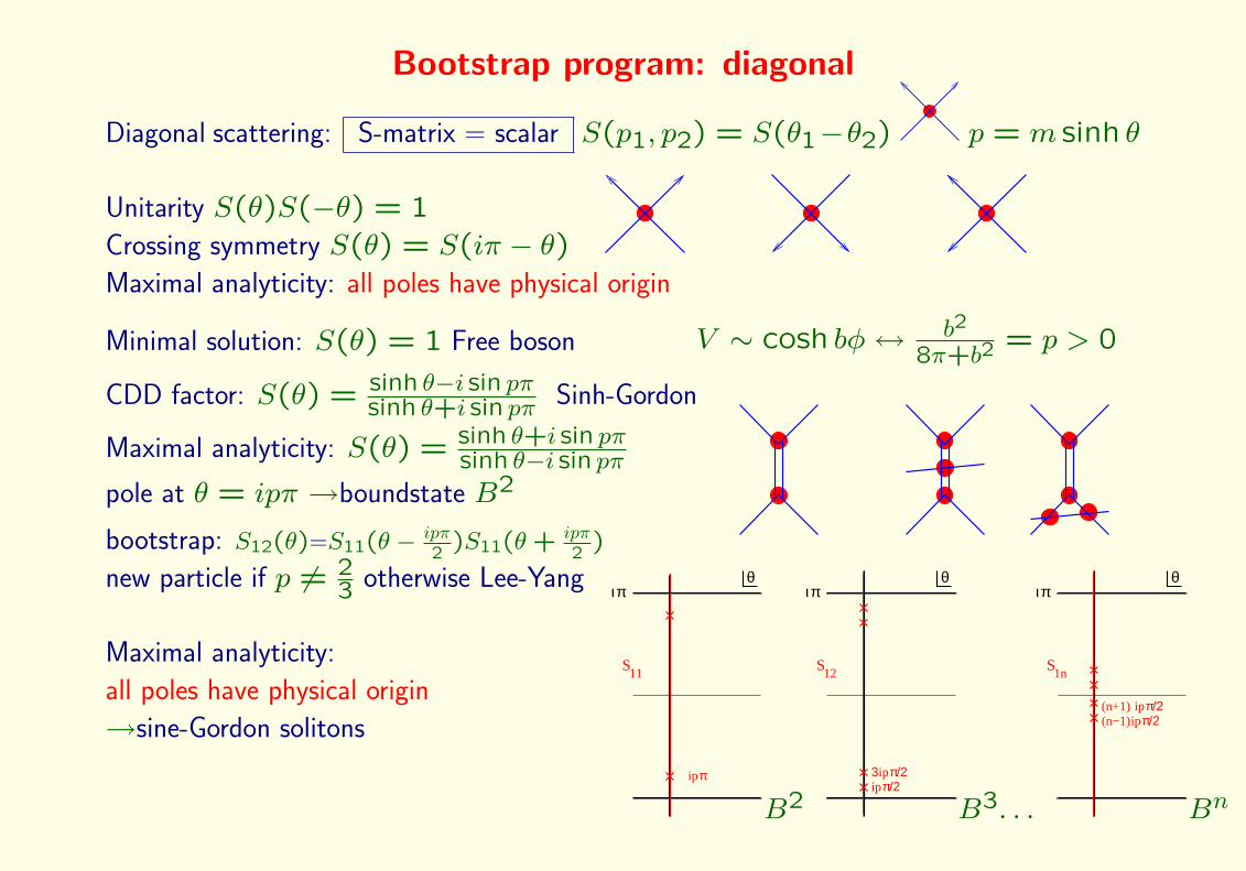
Bootstrap program: diagonal
Diagonal scattering: S-matrix = scalar S(p1, p2) = S(θ1−θ2) p = m sinh θ
Unitarity S(θ)S(−θ) = 1
Crossing symmetry S(θ) = S(iπ − θ)
Maximal analyticity: all poles have physical origin
Minimal solution: S(θ) = 1 Free boson
Bootstrap program: diagonal
Diagonal scattering: S-matrix = scalar S(p1, p2) = S(θ1−θ2) p = m sinh θ
Unitarity S(θ)S(−θ) = 1
Crossing symmetry S(θ) = S(iπ − θ)
Maximal analyticity: all poles have physical origin
Minimal solution: S(θ) = 1 Free boson
CDD factor: S(θ) = sinh θ−i sin pπsinh θ+i sin pπ

Bootstrap program: diagonal
Diagonal scattering: S-matrix = scalar S(p1, p2) = S(θ1−θ2) p = m sinh θ
Unitarity S(θ)S(−θ) = 1
Crossing symmetry S(θ) = S(iπ − θ)
Maximal analyticity: all poles have physical origin
Minimal solution: S(θ) = 1 Free boson
CDD factor: S(θ) = sinh θ−i sin pπsinh θ+i sin pπ Sinh-Gordon
V ∼ cosh bφ↔ b2
8π+b2= p > 0
Maximal analyticity: S(θ) = sinh θ+i sin pπsinh θ−i sin pπ
pole at θ = ipπ →boundstate B2
bootstrap: S12(θ)=S11(θ − ipπ2
)S11(θ + ipπ2
)
new particle if p 6= 23 otherwise Lee-Yang
Bootstrap program: diagonal
Diagonal scattering: S-matrix = scalar S(p1, p2) = S(θ1−θ2) p = m sinh θ
Unitarity S(θ)S(−θ) = 1Crossing symmetry S(θ) = S(iπ − θ)Maximal analyticity: all poles have physical origin
Minimal solution: S(θ) = 1 Free boson
CDD factor: S(θ) = sinh θ−i sin pπsinh θ+i sin pπ Sinh-Gordon
V ∼ cosh bφ↔ b2
8π+b2= p > 0
Maximal analyticity: S(θ) = sinh θ+i sin pπsinh θ−i sin pπ
pole at θ = ipπ →boundstate B2
bootstrap: S12(θ)=S11(θ − ipπ2
)S11(θ + ipπ2
)
new particle if p 6= 23 otherwise Lee-Yang
Maximal analyticity:
all poles have physical origin
→sine-Gordon solitons
θιπ
S11
ipπ
B2
θιπ
S
ipπ/23ipπ/2
12
B3. . .
θιπ
S1n
π/2ip(n+1)(n−1)ipπ/2
Bn

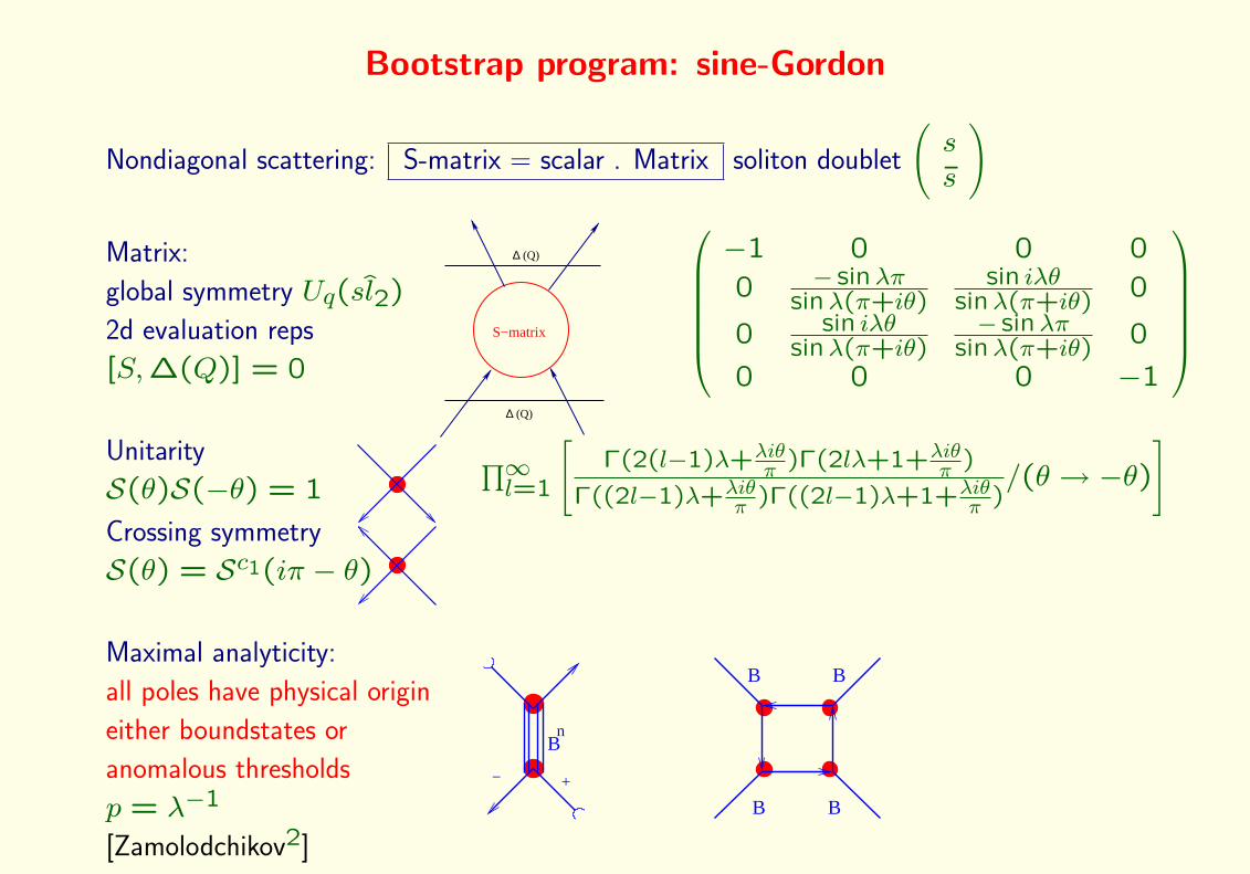
Bootstrap program: sine-Gordon
Nondiagonal scattering: S-matrix = scalar . Matrix soliton doublet
(ss
)
Matrix:
global symmetry Uq(sl2)
2d evaluation reps
[S,∆(Q)] = 0S−matrix
(Q)∆
∆ (Q)
−1 0 0 0
0 − sinλπsinλ(π+iθ)
sin iλθsinλ(π+iθ) 0
0 sin iλθsinλ(π+iθ)
− sinλπsinλ(π+iθ) 0
0 0 0 −1
9

Bootstrap program: sine-Gordon
Nondiagonal scattering: S-matrix = scalar . Matrix soliton doublet
(ss
)
Matrix:
global symmetry Uq(sl2)
2d evaluation reps
[S,∆(Q)] = 0S−matrix
(Q)∆
∆ (Q)
−1 0 0 0
0 − sinλπsinλ(π+iθ)
sin iλθsinλ(π+iθ) 0
0 sin iλθsinλ(π+iθ)
− sinλπsinλ(π+iθ) 0
0 0 0 −1
Unitarity
S(θ)S(−θ) = 1
Crossing symmetry
S(θ) = Sc1(iπ − θ)
∏∞l=1
[Γ(2(l−1)λ+λiθ
π )Γ(2lλ+1+λiθπ )
Γ((2l−1)λ+λiθπ )Γ((2l−1)λ+1+λiθ
π )/(θ → −θ)
]
Bootstrap program: sine-Gordon
Nondiagonal scattering: S-matrix = scalar . Matrix soliton doublet
(ss
)
Matrix:
global symmetry Uq(sl2)2d evaluation reps
[S,∆(Q)] = 0
S−matrix
(Q)∆
∆ (Q)
−1 0 0 0
0 − sinλπsinλ(π+iθ)
sin iλθsinλ(π+iθ) 0
0 sin iλθsinλ(π+iθ)
− sinλπsinλ(π+iθ) 0
0 0 0 −1
Unitarity
S(θ)S(−θ) = 1
Crossing symmetry
S(θ) = Sc1(iπ − θ)
∏∞l=1
[Γ(2(l−1)λ+λiθ
π )Γ(2lλ+1+λiθπ )
Γ((2l−1)λ+λiθπ )Γ((2l−1)λ+1+λiθ
π )/(θ → −θ)
]
Maximal analyticity:
all poles have physical origin
either boundstates or
anomalous thresholds
p = λ−1
[Zamolodchikov2]
+−
Bn
B
B B
B

Bootstrap program: sine-Gordon
Nondiagonal scattering: S-matrix = scalar . Matrix soliton doublet
(ss
)
Matrix:
global symmetry Uq(sl2)2d evaluation reps
[S,∆(Q)] = 0
S−matrix
(Q)∆
∆ (Q)
−1 0 0 0
0 − sinλπsinλ(π+iθ)
sin iλθsinλ(π+iθ) 0
0 sin iλθsinλ(π+iθ)
− sinλπsinλ(π+iθ) 0
0 0 0 −1
Unitarity
S(θ)S(−θ) = 1Crossing symmetry
S(θ) = Sc1(iπ − θ)
∏∞l=1
[Γ(2(l−1)λ+λiθ
π )Γ(2lλ+1+λiθπ )
Γ((2l−1)λ+λiθπ )Γ((2l−1)λ+1+λiθ
π )/(θ → −θ)
]
Maximal analyticity:
all poles have physical origin
either boundstates or
anomalous thresholds
p = λ−1
[Zamolodchikov2]
+−
Bn
B
B B
B
θιπ
S+−+−
(1−np)ιπ
...
...

Bootstrap program: AdS g
Classical string theory
Semiclassical string theory
J
1 loop perturbative gauge theory
+ string loop corrections
Nonperturbative gauge theory
Quantum String theory
S −
mat
rix
+ gauge loop corrections
Asy
mpt
otic
Bet
he A
nsat
z
Wra
ppin
g/Lu
sche
r co
rrec
tion
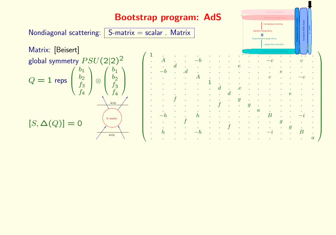
Nondiagonal scattering: S-matrix = scalar . Matrix
10

Bootstrap program: AdS g
Classical string theory
Semiclassical string theory
J
1 loop perturbative gauge theory
+ string loop corrections
Nonperturbative gauge theory
Quantum String theory
S −
mat
rix
+ gauge loop corrections
Asy
mpt
otic
Bet
he A
nsat
z
Wra
ppin
g/Lu
sche
r co
rrec
tion
Nondiagonal scattering: S-matrix = scalar . Matrix
Matrix: [Beisert]
global symmetry PSU(2|2)2
Q = 1 reps
b1
b2
f3
f4
⊗ b1
b2f3f4
[S,∆(Q)] = 0S−matrix
(Q)∆
∆ (Q)
1 . . . . . . . . . . . . . . .. A . . −b . . . . . . −c . . c .. . d . . . . . e . . . . . . .. −b . .d . . . . . . . . e . . .. . . . A . . . . . . c . . −c .. . . . . 1 . . . . . . . . . .. . . . . . d . .e . . . . . . .. . . . . . . d . . . . . e . .. . f . . . . . g . . . . . . .. . . . . . f . . g . . . . . .. . . . . . . . . . a . . . . .. −h . . h . . . . . . B . . −i .. . . f . . . . . . . . g . . .. . . . . . . f . . . . . g . .. h . . −h . . . . . . −i . . B .. . . . . . . . . . . . . . . a
Unitarity
S(z1, z2)S(z2, z1) = 1
Crossing symmetry [Janik] [Volin]
S(z1, z2) = Sc1(z2, z1 + ω2)
S1111 = u1−u2−i
u1−u2+iei2θ(z1,z2)
u = 12
cot p2E(p)
[Beisert,Eden,Staudacher]
p = 2 am(z)

Bootstrap program: AdSg
Classical string theory
Semiclassical string theory
J
1 loop perturbative gauge theory
+ string loop corrections
Nonperturbative gauge theory
Quantum String theory
S −
mat
rix
+ gauge loop corrections
Asy
mpt
otic
Bet
he A
nsat
z
Wra
ppin
g/Lu
sche
r co
rrec
tion
Nondiagonal scattering: S-matrix = scalar . Matrix
Matrix: [Beisert]
global symmetry PSU(2|2)2
Q = 1 reps
b1
b2
f3
f4
⊗ b1
b2f3f4
[S,∆(Q)] = 0S−matrix
(Q)∆
∆ (Q)
1 . . . . . . . . . . . . . . .. A . . −b . . . . . . −c . . c .. . d . . . . . e . . . . . . .. −b . .d . . . . . . . . e . . .. . . . A . . . . . . c . . −c .. . . . . 1 . . . . . . . . . .. . . . . . d . .e . . . . . . .. . . . . . . d . . . . . e . .. . f . . . . . g . . . . . . .. . . . . . f . . g . . . . . .. . . . . . . . . . a . . . . .. −h . . h . . . . . . B . . −i .. . . f . . . . . . . . g . . .. . . . . . . f . . . . . g . .. h . . −h . . . . . . −i . . B .. . . . . . . . . . . . . . . a
Unitarity
S(z1, z2)S(z2, z1) = 1Crossing symmetry [Janik] [Volin]
S(z1, z2) = Sc1(z2, z1 + ω2)
S1111 = u1−u2−i
u1−u2+iei2θ(z1,z2)
u = 12
cot p2E(p)
[Beisert,Eden,Staudacher]
p = 2 am(z)
Maximal analyticity:
boundstates atyp symrep: Q ∈ N
anomalous thresholds Physical domain?
[N.Dorey,Maldacena,Hofman,Okamura] [Frolov]1 Q
Q 1
1Q ω /2
−ω /2 ω /2
ω2
2
1 1

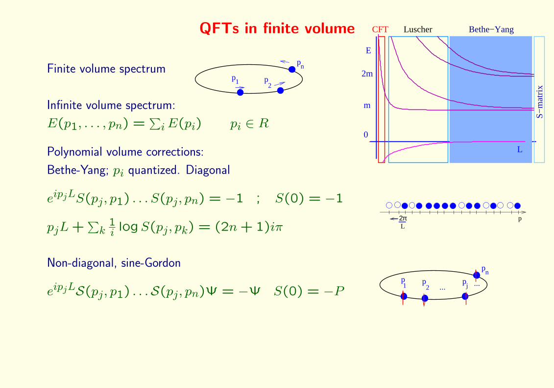
QFTs in finite volume
Finite volume spectrump
2p
n
p1
11

QFTs in finite volume
Finite volume spectrump
2p
n
p1
L
E
0
2m
m
S−
mat
rix
Bethe−YangLuscherCFT

QFTs in finite volume
Finite volume spectrump
2p
n
p1
L
E
0
2m
m
S−
mat
rix
Bethe−YangLuscherCFT

QFTs in finite volume
Finite volume spectrump
2p
n
p1
L
E
0
2m
m
S−
mat
rix
Bethe−YangLuscherCFT
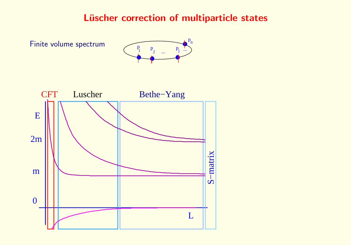
Infinite volume spectrum:
E(p1, . . . , pn) =∑iE(pi) pi ∈ R

QFTs in finite volume
Finite volume spectrump
2p
n
p1
L
E
0
2m
m
S−
mat
rix
Bethe−YangLuscherCFT
Infinite volume spectrum:
E(p1, . . . , pn) =∑iE(pi) pi ∈ R
Polynomial volume corrections:
Bethe-Yang; pi quantized. Diagonal

QFTs in finite volume
Finite volume spectrump
2p
n
p1
L
E
0
2m
m
S−
mat
rix
Bethe−YangLuscherCFT
Infinite volume spectrum:
E(p1, . . . , pn) =∑iE(pi) pi ∈ R
Polynomial volume corrections:
Bethe-Yang; pi quantized. Diagonal
eipjLS(pj, p1) . . . S(pj, pn) = −1 ; S(0) = −1
pjL+∑k
1i logS(pj, pk) = (2n+ 1)iπ
p2πL
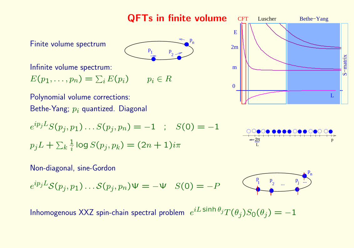
Non-diagonal, sine-Gordon
eipjLS(pj, p1) . . .S(pj, pn)Ψ = −Ψ S(0) = −Pn
1 2 j... ...p p p
p
QFTs in finite volume
Finite volume spectrump
2p
n
p1
L
E
0
2m
m
S−
mat
rix
Bethe−YangLuscherCFT
Infinite volume spectrum:
E(p1, . . . , pn) =∑iE(pi) pi ∈ R
Polynomial volume corrections:
Bethe-Yang; pi quantized. Diagonal
eipjLS(pj, p1) . . . S(pj, pn) = −1 ; S(0) = −1
pjL+∑k
1i logS(pj, pk) = (2n+ 1)iπ
p2πL
Non-diagonal, sine-Gordon
eipjLS(pj, p1) . . .S(pj, pn)Ψ = −Ψ S(0) = −Pn
1 2 j... ...p p p
p
Inhomogenous XXZ spin-chain spectral problem eiL sinh θjT (θj)S0(θj) = −1
T (θ)Q(θ) = Q(θ+iπ)T0(θ− iπ2 )+Q(θ−iπ)T0(θ+ iπ2 ) = Q++T−+Q−−T+

QFTs in finite volume
Finite volume spectrump
2p
n
p1
L
E
0
2m
m
S−
mat
rix
Bethe−YangLuscherCFT
Infinite volume spectrum:
E(p1, . . . , pn) =∑iE(pi) pi ∈ R
Polynomial volume corrections:
Bethe-Yang; pi quantized. Diagonal
eipjLS(pj, p1) . . . S(pj, pn) = −1 ; S(0) = −1
pjL+∑k
1i logS(pj, pk) = (2n+ 1)iπ
p2πL
Non-diagonal, sine-Gordon
eipjLS(pj, p1) . . .S(pj, pn)Ψ = −Ψ S(0) = −P
n
1 2 j... ...p p p
p
Inhomogenous XXZ spin-chain spectral problem eiL sinh θjT (θj)S0(θj) = −1
T (θ)Q(θ) = Q(θ+iπ)T0(θ− iπ2 )+Q(θ−iπ)T0(θ+ iπ2 ) = Q++T−+Q−−T+
Q(θ) =∏β sinh(λ(θ − wβ))
T0(θ) =∏j sinh(λ(θ − θj))
Bethe Ansatz:T0(wα−iπ2 )Q(wα+iπ)
T0(wα+iπ2 )Q(wα−iπ)
=T−0 Q
++
T+0 Q−−
|α = −1
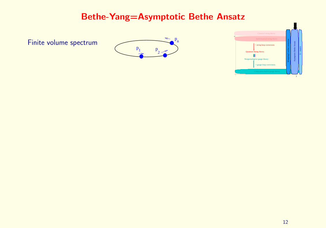
Bethe-Yang=Asymptotic Bethe Ansatz
g
Classical string theory
Semiclassical string theory
J
1 loop perturbative gauge theory
+ string loop corrections
Nonperturbative gauge theory
Quantum String theory
S −
mat
rix
+ gauge loop corrections
Asy
mpt
otic
Bet
he A
nsat
z
Wra
ppin
g/Lu
sche
r co
rrec
tion
Finite volume spectrump
2p
n
p1
12

Bethe-Yang=Asymptotic Bethe Ansatz
g
Classical string theory
Semiclassical string theory
J
1 loop perturbative gauge theory
+ string loop corrections
Nonperturbative gauge theory
Quantum String theory
S −
mat
rix
+ gauge loop corrections
Asy
mpt
otic
Bet
he A
nsat
z
Wra
ppin
g/Lu
sche
r co
rrec
tion
Finite volume spectrump
2p
n
p1
Infinite volume spectrum:
E(p1, . . . , pn) =∑iE(pi) E(p) =
√1 + (4g sin p
2)2 pi ∈ [−π, π]

Bethe-Yang=Asymptotic Bethe Ansatz
g
Classical string theory
Semiclassical string theory
J
1 loop perturbative gauge theory
+ string loop corrections
Nonperturbative gauge theory
Quantum String theory
S −
mat
rix
+ gauge loop corrections
Asy
mpt
otic
Bet
he A
nsat
z
Wra
ppin
g/Lu
sche
r co
rrec
tionFinite volume spectrum
p
2p
n
p1
Infinite volume spectrum:
E(p1, . . . , pn) =∑iE(pi) E(p) =
√1 + (4g sin p
2)2 pi ∈ [−π, π]
Polynomial volume corrections:
Asymptotic Bethe Ansatz; pi quantized, .
eipjLS(pj, p1) . . .S(pj, pn)Ψ = −Ψ S(0) = −Pn
1 2 j... ...p p p
p

Bethe-Yang=Asymptotic Bethe Ansatz
g
Classical string theory
Semiclassical string theory
J
1 loop perturbative gauge theory
+ string loop corrections
Nonperturbative gauge theory
Quantum String theory
S −
mat
rix
+ gauge loop corrections
Asy
mpt
otic
Bet
he A
nsat
z
Wra
ppin
g/Lu
sche
r co
rrec
tion
Finite volume spectrump
2p
n
p1
Infinite volume spectrum:
E(p1, . . . , pn) =∑iE(pi) E(p) =
√1 + (4g sin p
2)2 pi ∈ [−π, π]
Polynomial volume corrections:
Asymptotic Bethe Ansatz; pi quantized, .
eipjLS(pj, p1) . . .S(pj, pn)Ψ = −Ψ S(0) = −Pn
1 2 j... ...p p p
p
Inhomogenous Hubbard2 spin-chain: eiLpjS20(uj)
Q++4 (uj)
Q−−4 (uj)T (uj)T (uj) = −1

Bethe-Yang=Asymptotic Bethe Ansatz
g
Classical string theory
Semiclassical string theory
J
1 loop perturbative gauge theory
+ string loop corrections
Nonperturbative gauge theory
Quantum String theory
S −
mat
rix
+ gauge loop corrections
Asy
mpt
otic
Bet
he A
nsat
z
Wra
ppin
g/Lu
sche
r co
rrec
tionFinite volume spectrum
p
2p
n
p1
Infinite volume spectrum:
E(p1, . . . , pn) =∑iE(pi) E(p) =
√1 + (4g sin p
2)2 pi ∈ [−π, π]
Polynomial volume corrections:
Asymptotic Bethe Ansatz; pi quantized, .
eipjLS(pj, p1) . . .S(pj, pn)Ψ = −Ψ S(0) = −Pn
1 2 j... ...p p p
p
Inhomogenous Hubbard2 spin-chain: eiLpjS20(uj)
Q++4 (uj)
Q−−4 (uj)T (uj)T (uj) = −1
T (u) =B−1 B
+3 R−(+)4
B+1 B−3 R−(−)4
[Q−−2 Q+
3Q2Q
−3− R
−(−)4 Q+
3
R−(+)4 Q−3
+Q++
2 Q−1Q2Q
+1
− B+(+)4 Q−1
B+(−)4 Q+
1
][Beisert,Staudacher]
Qj(u) = −Rj(u)Bj(u) andR(±)j =
∏k
x(u)−x∓j,k√x∓j,k
B(±)j =
∏k
1
x(u)−x∓j,k√x∓j,k
[Kazakov,Gromov]

Bethe-Yang=Asymptotic Bethe Ansatz
g
Classical string theory
Semiclassical string theory
J
1 loop perturbative gauge theory
+ string loop corrections
Nonperturbative gauge theory
Quantum String theory
S −
mat
rix
+ gauge loop corrections
Asy
mpt
otic
Bet
he A
nsat
z
Wra
ppin
g/Lu
sche
r co
rrec
tionFinite volume spectrum
p
2p
n
p1
Infinite volume spectrum:
E(p1, . . . , pn) =∑iE(pi) E(p) =
√1 + (4g sin p
2)2 pi ∈ [−π, π]
Polynomial volume corrections:
Asymptotic Bethe Ansatz; pi quantized, .
eipjLS(pj, p1) . . .S(pj, pn)Ψ = −Ψ S(0) = −P
n
1 2 j... ...p p p
p
Inhomogenous Hubbard2 spin-chain: eiLpjS20(uj)
Q++4 (uj)
Q−−4 (uj)T (uj)T (uj) = −1
T (u) =B−1 B
+3 R−(+)4
B+1 B−3 R−(−)4
[Q−−2 Q+
3Q2Q
−3− R
−(−)4 Q+
3
R−(+)4 Q−3
+Q++
2 Q−1Q2Q
+1
− B+(+)4 Q−1
B+(−)4 Q+
1
][Beisert,Staudacher]
Qj(u) = −Rj(u)Bj(u) andR(±)j =
∏k
x(u)−x∓j,k√x∓j,k
B(±)j =
∏k
1
x(u)−x∓j,k√x∓j,k
[Kazakov,Gromov]
Bethe Ansatz:Q+
2 B(−)4
Q−2B(+)4
|1 = 1Q−−2 Q+
1 Q+3
Q++2 Q−1Q
−3
|2 = −1Q+
2 R(−)4
Q−2R(+)4
|3 = 1 [Frolov]

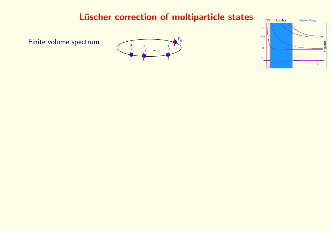
Luscher correction of multiparticle states
Finite volume spectrum n
1 2 j... ...p p p
p
13
Luscher correction of multiparticle states
Finite volume spectrum n
1 2 j... ...p p p
p
L
E
0
2m
m
S−
mat
rix
Bethe−YangLuscherCFT
Luscher correction of multiparticle states
Finite volume spectrum n
1 2 j... ...p p p
p
L
E
0
2m
m
S−
mat
rix
Bethe−YangLuscherCFT

Luscher correction of multiparticle states
Finite volume spectrum n
1 2 j... ...p p p
p
L
E
0
2m
m
S−
mat
rix
Bethe−YangLuscherCFT
Luscher originally: O(e−mL) mass correction
m(L) =√
32 m(−iRes
θ=2iπ3S)e−
√3
2 mL
−∫ dθ
2π cosh θ(S(θ + iπ2 )− 1)e−mL cosh θ

Luscher correction of multiparticle states
Finite volume spectrum n
1 2 j... ...p p p
p
L
E
0
2m
m
S−
mat
rix
Bethe−YangLuscherCFT
Luscher originally: O(e−mL) mass correction
m(L) =√
32 m(−iRes
θ=2iπ3S)e−
√3
2 mL
−∫ dθ
2π cosh θ(S(θ + iπ2 )− 1)e−mL cosh θ
Multiparticle Luscher correction [ZB,Janik]
BY: S(pj, p1) . . .S(pj, pn)Ψ = −e−ipjLΨ
T (p, p1, . . . , pn)Ψ = t(p, p1, . . . , pn,Ψ)Ψ
Modified momenta:
pjL− i log t(pj, p1, . . . , pn,Ψ) = (2n+ 1)π + Φj
Φj =∫ dq
2πddpjt(q, p1, . . . , pn,Ψ)e−LE(q)

Luscher correction of multiparticle states
Finite volume spectrumn
1 2 j... ...p p p
p
L
E
0
2m
m
S−
mat
rix
Bethe−YangLuscherCFT
Luscher originally: O(e−mL) mass correction
m(L) =√
32 m(−iRes
θ=2iπ3S)e−
√3
2 mL
−∫ dθ
2π cosh θ(S(θ + iπ2 )− 1)e−mL cosh θ
Multiparticle Luscher correction [ZB,Janik]
BY: S(pj, p1) . . .S(pj, pn)Ψ = −e−ipjLΨT (p, p1, . . . , pn)Ψ = t(p, p1, . . . , pn,Ψ)Ψ
Modified momenta:
pjL− i log t(pj, p1, . . . , pn,Ψ) = (2n+ 1)π + Φj
Φj =∫ dq
2πddpjt(q, p1, . . . , pn,Ψ)e−LE(q)
Modified energy:
E(p1, . . . , pn) =∑kE(pk + δpk)−
∫ dq2πt(q, p1, . . . , pn,Ψ)e−LE(q)

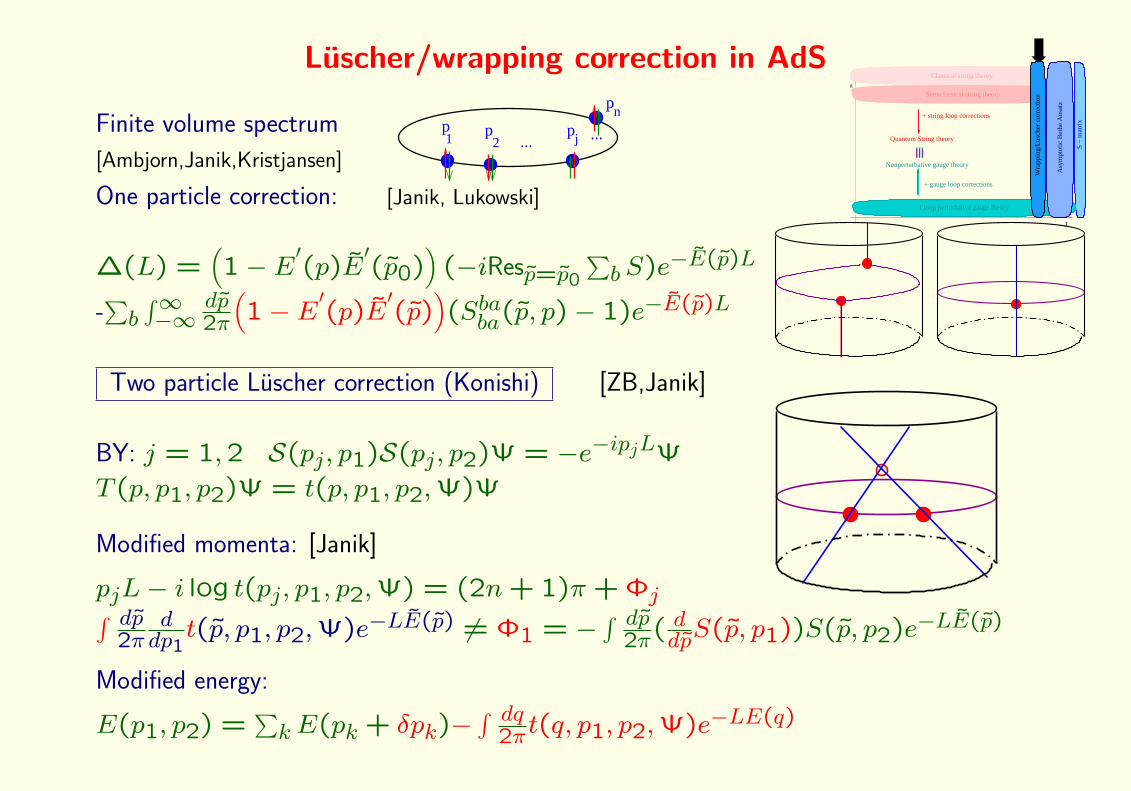
Luscher/wrapping correction in AdSg
Classical string theory
Semiclassical string theory
J
1 loop perturbative gauge theory
+ string loop corrections
Nonperturbative gauge theory
Quantum String theory
S −
mat
rix
+ gauge loop corrections
Asy
mpt
otic
Bet
he A
nsat
z
Wra
ppin
g/Lu
sche
r co
rrec
tion
Finite volume spectrum
[Ambjorn,Janik,Kristjansen]
n
1 2 j... ...p p p
p
14

Luscher/wrapping correction in AdSg
Classical string theory
Semiclassical string theory
J
1 loop perturbative gauge theory
+ string loop corrections
Nonperturbative gauge theory
Quantum String theory
S −
mat
rix
+ gauge loop corrections
Asy
mpt
otic
Bet
he A
nsat
z
Wra
ppin
g/Lu
sche
r co
rrec
tion
Finite volume spectrum
[Ambjorn,Janik,Kristjansen]
n
1 2 j... ...p p p
p
One particle correction: [Janik, Lukowski]
∆(L) =(1− E′(p)E
′(p0)
)(−iResp=p0
∑b S)e−E(p)L
-∑b∫∞−∞
dp2π
(1− E′(p)E
′(p)
)(Sbaba(p, p)− 1)e−E(p)L
Two particle Luscher correction (Konishi) [ZB,Janik]
BY: j = 1,2 S(pj, p1)S(pj, p2)Ψ = −e−ipjLΨ
T (p, p1, p2)Ψ = t(p, p1, p2,Ψ)Ψ
Modified momenta: [Janik]
pjL− i log t(pj, p1, p2,Ψ) = (2n+ 1)π + Φj∫ dp2π
ddp1
t(p, p1, p2,Ψ)e−LE(p) 6= Φ1 = −∫ dp
2π( ddpS(p, p1))S(p, p2)e−LE(p)
Modified energy:
E(p1, p2) =∑kE(pk + δpk)−
∫ dq2πt(q, p1, p2,Ψ)e−LE(q)

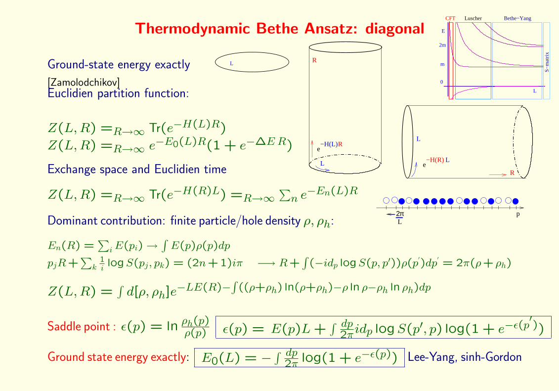
Thermodynamic Bethe Ansatz: diagonal
Ground-state energy exactly
[Zamolodchikov]
L
15

Thermodynamic Bethe Ansatz: diagonal
Ground-state energy exactly
[Zamolodchikov]
L
L
E
0
2m
m
S−
mat
rix
Bethe−YangLuscherCFT

Thermodynamic Bethe Ansatz: diagonal
Ground-state energy exactly
[Zamolodchikov]
L
L
E
0
2m
m
S−
mat
rix
Bethe−YangLuscherCFT

Thermodynamic Bethe Ansatz: diagonal
Ground-state energy exactly
[Zamolodchikov]
L
L
E
0
2m
m
S−
mat
rix
Bethe−YangLuscherCFT
Euclidien partition function:
Z(L,R) =R→∞ Tr(e−H(L)R)
Z(L,R) =R→∞ e−E0(L)R(1 + e−∆ER)
L
e−H(L)R
R

Thermodynamic Bethe Ansatz: diagonal
Ground-state energy exactly
[Zamolodchikov]
L
L
E
0
2m
m
S−
mat
rix
Bethe−YangLuscherCFT
Euclidien partition function:
Z(L,R) =R→∞ Tr(e−H(L)R)
Z(L,R) =R→∞ e−E0(L)R(1 + e−∆ER)
L
e−H(L)R
R
Exchange space and Euclidien time
Z(L,R) =R→∞ Tr(e−H(R)L) =R→∞∑n e−En(L)R
L
Re−H(R) L
Dominant contribution: finite particle/hole density ρ, ρh:p2π
L
En(R) =∑
iE(pi)→∫E(p)ρ(p)dp
pjR+∑
k1i
logS(pj, pk) = (2n+ 1)iπ −→ R+∫
(−idp logS(p, p′))ρ(p′)dp
′= 2π(ρ+ ρh)
Z(L,R) =∫d[ρ, ρh]e−LE(R)−
∫((ρ+ρh) ln(ρ+ρh)−ρ ln ρ−ρh ln ρh)dp
Thermodynamic Bethe Ansatz: diagonal
Ground-state energy exactly
[Zamolodchikov]
L
L
E
0
2m
m
S−
mat
rix
Bethe−YangLuscherCFT
Euclidien partition function:
Z(L,R) =R→∞ Tr(e−H(L)R)
Z(L,R) =R→∞ e−E0(L)R(1 + e−∆ER)L
e−H(L)R
R
Exchange space and Euclidien time
Z(L,R) =R→∞ Tr(e−H(R)L) =R→∞∑n e−En(L)R
L
Re−H(R) L
Dominant contribution: finite particle/hole density ρ, ρh:p2π
L
En(R) =∑
iE(pi)→∫E(p)ρ(p)dp
pjR+∑
k1i
logS(pj, pk) = (2n+ 1)iπ −→ R+∫
(−idp logS(p, p′))ρ(p′)dp
′= 2π(ρ+ ρh)
Z(L,R) =∫d[ρ, ρh]e−LE(R)−
∫((ρ+ρh) ln(ρ+ρh)−ρ ln ρ−ρh ln ρh)dp
Saddle point : ε(p) = ln ρh(p)ρ(p) ε(p) = E(p)L+
∫ dp2πidp logS(p′, p) log(1 + e−ε(p
′))
Ground state energy exactly: E0(L) = −∫ dp
2π log(1 + e−ε(p)) Lee-Yang, sinh-Gordon

Thermodynamic Bethe Ansatz: non-diagonal
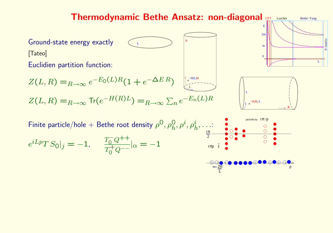
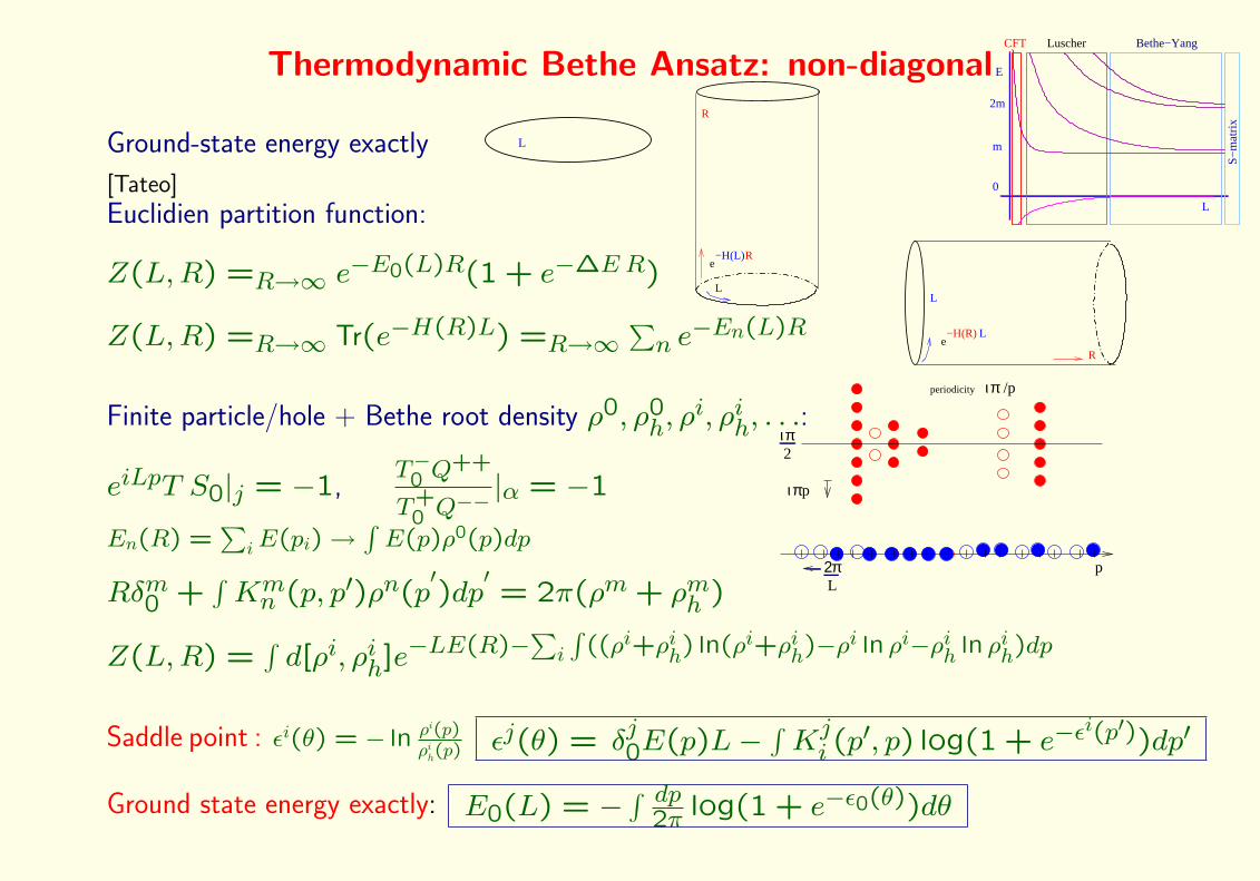
Ground-state energy exactly
[Tateo]
L
L
E
0
2m
m
S−
mat
rix
Bethe−YangLuscherCFT
Euclidien partition function:
Z(L,R) =R→∞ e−E0(L)R(1 + e−∆ER)L
e−H(L)R
R
Z(L,R) =R→∞ Tr(e−H(R)L) =R→∞∑n e−En(L)R
L
Re−H(R) L
16
Thermodynamic Bethe Ansatz: non-diagonal
Ground-state energy exactly
[Tateo]
L
L
E
0
2m
m
S−
mat
rix
Bethe−YangLuscherCFT
Euclidien partition function:
Z(L,R) =R→∞ e−E0(L)R(1 + e−∆ER)L
e−H(L)R
R
Z(L,R) =R→∞ Tr(e−H(R)L) =R→∞∑n e−En(L)R
L
Re−H(R) L
Finite particle/hole + Bethe root density ρ0, ρ0h, ρ
i, ρih, . . .:
eiLpT S0|j = −1,T−0 Q
++
T+0 Q−−
|α = −1
p2πL
ιπ2
ιπp
periodicity ιπ /p
En(R) =∑
iE(pi)→∫E(p)ρ0(p)dp
Rδm0 +∫Kmn (p, p′)ρn(p
′)dp
′= 2π(ρm + ρmh )
Z(L,R) =∫d[ρi, ρih]e−LE(R)−
∑i
∫((ρi+ρih) ln(ρi+ρih)−ρi ln ρi−ρih ln ρih)dp
Saddle point : εi(θ) = − ln ρi(p)ρih(p) εj(θ) = δ
j0E(p)L−
∫Kji (p′, p) log(1 + e−ε
i(p′))dp′
Ground state energy exactly: E0(L) = −∫ dp
2π log(1 + e−ε0(θ))dθ
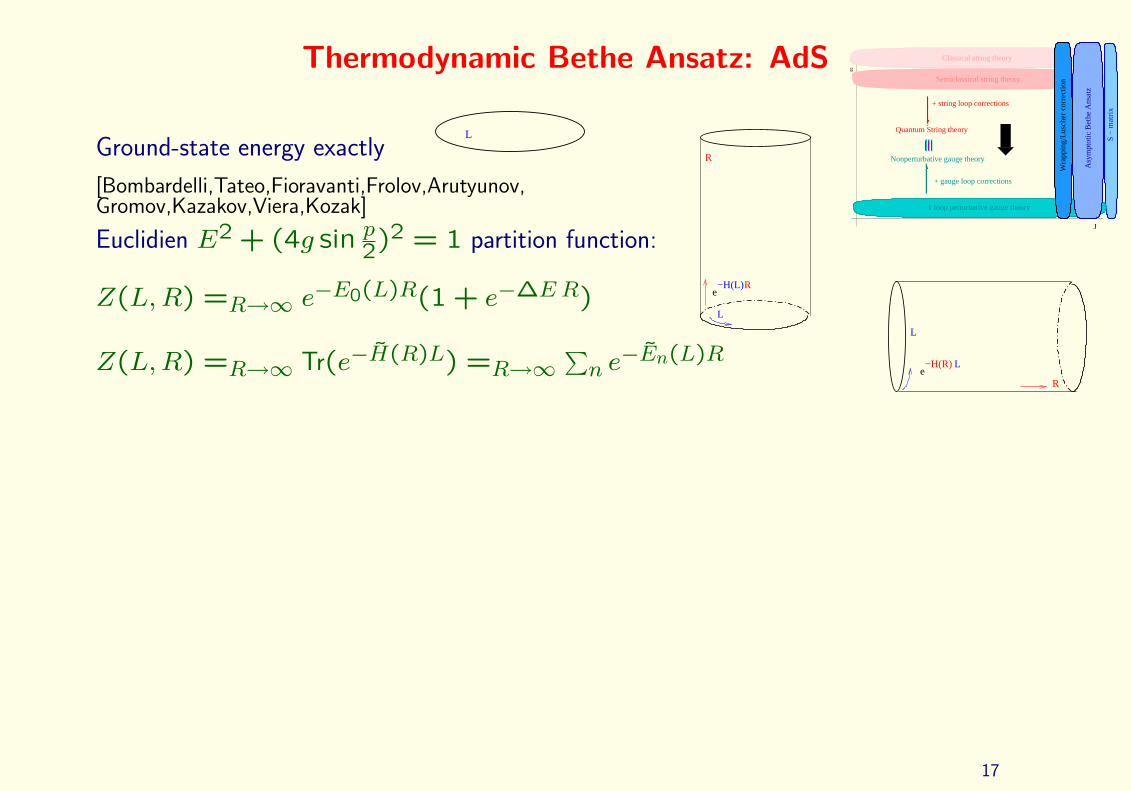
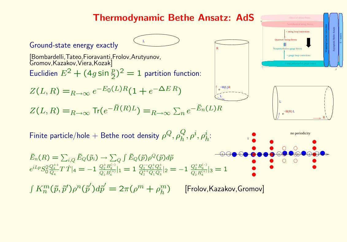
Thermodynamic Bethe Ansatz: AdS g
Classical string theory
Semiclassical string theory
J
1 loop perturbative gauge theory
+ string loop corrections
Nonperturbative gauge theory
Quantum String theory
S −
mat
rix
+ gauge loop corrections
Asy
mpt
otic
Bet
he A
nsat
z
Wra
ppin
g/Lu
sche
r co
rrec
tion
Ground-state energy exactly
[Bombardelli,Tateo,Fioravanti,Frolov,Arutyunov,Gromov,Kazakov,Viera,Kozak]
L
Euclidien E2 + (4g sin p2)2 = 1 partition function:
Z(L,R) =R→∞ e−E0(L)R(1 + e−∆ER)L
e−H(L)R
R
Z(L,R) =R→∞ Tr(e−H(R)L) =R→∞∑n e−En(L)R
L
Re−H(R) L
17

Thermodynamic Bethe Ansatz: AdS g
Classical string theory
Semiclassical string theory
J
1 loop perturbative gauge theory
+ string loop corrections
Nonperturbative gauge theory
Quantum String theory
S −
mat
rix
+ gauge loop corrections
Asy
mpt
otic
Bet
he A
nsat
z
Wra
ppin
g/Lu
sche
r co
rrec
tion
Ground-state energy exactly
[Bombardelli,Tateo,Fioravanti,Frolov,Arutyunov,Gromov,Kazakov,Viera,Kozak]
L
Euclidien E2 + (4g sin p2)2 = 1 partition function:
Z(L,R) =R→∞ e−E0(L)R(1 + e−∆ER)L
e−H(L)R
R
Z(L,R) =R→∞ Tr(e−H(R)L) =R→∞∑n e−En(L)R
L
Re−H(R) L
Finite particle/hole + Bethe root density ρQ, ρQh , ρ
i, ρih: i
no periodicity
En(R) =∑
i,Q EQ(pi)→∑
Q
∫EQ(p)ρQ(p)dp
eiLpS20Q++
4
Q−−4
T T |4 = −1 Q+2 B
(−)4
Q−2B(+)4
|1 = 1 Q−−2 Q+1 Q
+3
Q++2 Q−1Q
−3
|2 = −1 Q+2 R
(−)4
Q−2R(+)4
|3 = 1
∫Kmn (p, p′)ρn(p
′)dp
′= 2π(ρm + ρmh ) [Frolov,Kazakov,Gromov]
Z(L,R) =∫d[ρi, ρih]e−LE(R)−
∑i
∫((ρi+ρih) ln(ρi+ρih)−ρi ln ρi−ρih ln ρih)dp
Saddle point : εi(p) = − ln ρi(p)ρih(p) εj(θ) = δ
jQEQ(p)L−
∫Kji (p, p′) log(1 + e−ε
i(p′))dp′
Ground state energy exactly: E0(L) = −∑Q∫ dp
2π log(1 + e−εQ(p))dp

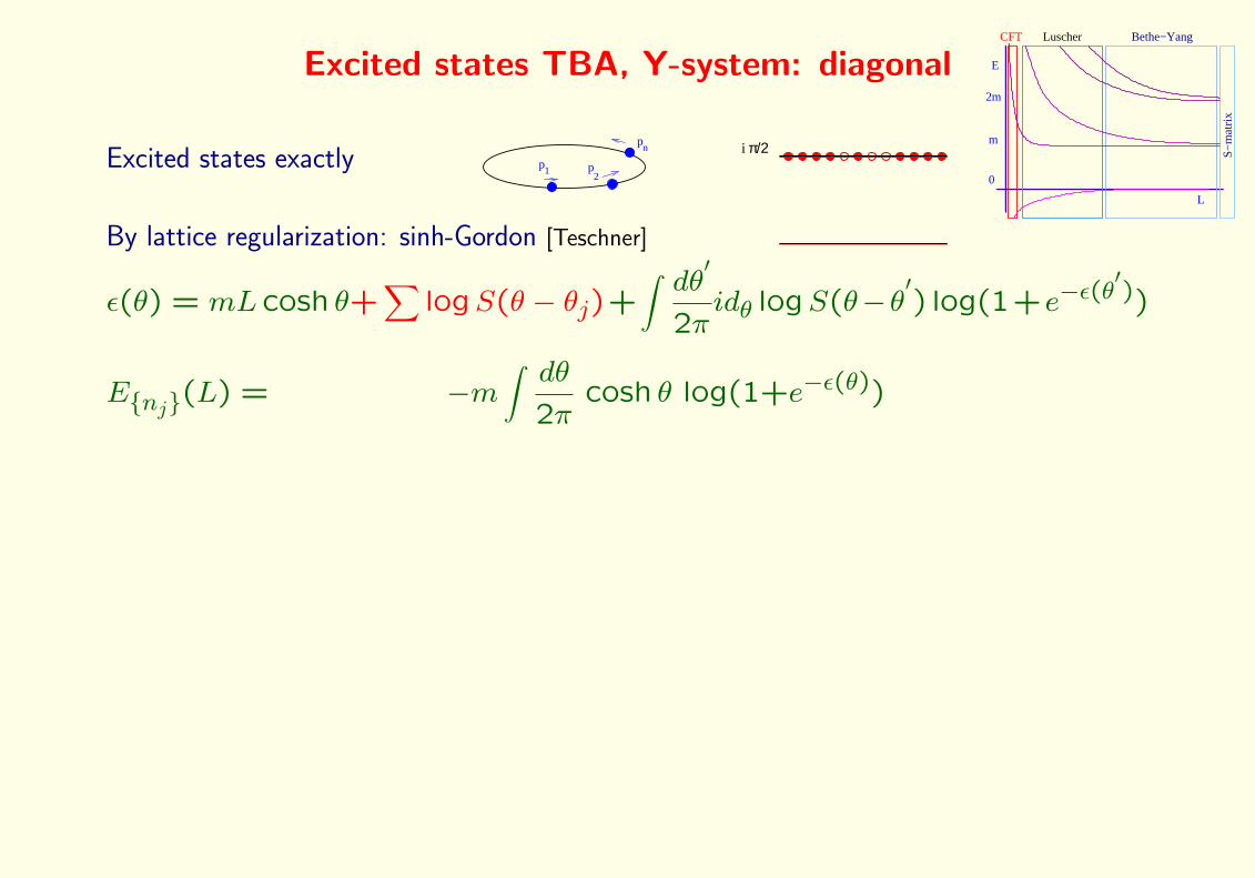
Excited states TBA, Y-system: diagonal
Excited states exactlyp
2p
n
p1
18

Excited states TBA, Y-system: diagonal
Excited states exactlyp
2p
n
p1
L
E
0
2m
m
S−
mat
rix
Bethe−YangLuscherCFT

Excited states TBA, Y-system: diagonal
Excited states exactlyp
2p
n
p1
L
E
0
2m
m
S−
mat
rix
Bethe−YangLuscherCFT
By lattice regularization: sinh-Gordon [Teschner]
i π/2
ε(θ) = mL cosh θ +∫dθ′
2πidθ logS(θ−θ
′) log(1+e−ε(θ
′))
E{nj}(L) = −m∫dθ
2πcosh θ log(1+e−ε(θ))
Excited states TBA, Y-system: diagonal
Excited states exactlyp
2p
n
p1
L
E
0
2m
m
S−
mat
rix
Bethe−YangLuscherCFT
By lattice regularization: sinh-Gordon [Teschner]
i π/2
ε(θ) = mL cosh θ+∑
logS(θ − θj)+∫dθ′
2πidθ logS(θ−θ
′) log(1+e−ε(θ
′))
E{nj}(L) = −m∫dθ
2πcosh θ log(1+e−ε(θ))

Excited states TBA, Y-system: diagonal
Excited states exactlyp
2p
n
p1
L
E
0
2m
m
S−
mat
rix
Bethe−YangLuscherCFT
By lattice regularization: sinh-Gordon [Teschner]
i π/2
ε(θ) = mL cosh θ+∑
logS(θ − θj)+∫dθ′
2πidθ logS(θ−θ
′) log(1+e−ε(θ
′))
E{nj}(L) =m
i
∑sinh θj−m
∫dθ
2πcosh θ log(1+e−ε(θ))

Excited states TBA, Y-system: diagonal
Excited states exactlyp
2p
n
p1
L
E
0
2m
m
S−
mat
rix
Bethe−YangLuscherCFT
By lattice regularization: sinh-Gordon [Teschner]
i π/2
ε(θ) = mL cosh θ+∑
logS(θ − θj)+∫dθ′
2πidθ logS(θ−θ
′) log(1+e−ε(θ
′))
E{nj}(L) =m
i
∑sinh θj−m
∫dθ
2πcosh θ log(1+e−ε(θ)) ; Y (θj) = eε(θj) = −1
By analytical continuation: Lee-Yang [P.Dorey,Tateo]
i π/6
π/6−i
ε(θ) = mL cosh θ +∫ ∞−∞
dθ′
2πidθ logS(θ−θ
′) log(1+e−ε(θ
′))
E{nj}(L) = −m∫ ∞−∞
dθ
2πcosh θ log(1 + e−ε(θ))
Luscher corrections: differ by µ term

Excited states TBA, Y-system: diagonal
Excited states exactlyp
2p
n
p1
L
E
0
2m
m
S−
mat
rix
Bethe−YangLuscherCFT
By lattice regularization: sinh-Gordon [Teschner]
i π/2
ε(θ) = mL cosh θ+∑
logS(θ − θj)+∫dθ′
2πidθ logS(θ−θ
′) log(1+e−ε(θ
′))
E{nj}(L) =m
i
∑sinh θj−m
∫dθ
2πcosh θ log(1+e−ε(θ)) ; Y (θj) = eε(θj) = −1
By analytical continuation: Lee-Yang [P.Dorey,Tateo]
i π/6
π/6−i
ε(θ) = mL cosh θ+N∑j=1
logS(θ − θj)S(θ − θ∗j)
+∫ ∞−∞
dθ′
2πidθ logS(θ−θ
′) log(1+e−ε(θ
′))
E{nj}(L) = −im∑
(sinh θj − sinh θ∗j)−m∫ ∞−∞
dθ
2πcosh θ log(1 + e−ε(θ))
Luscher corrections: differ by µ term
S(θ − iπ3 )S(θ + iπ
3 ) = S(θ)→ Y (θ + iπ3 )Y (θ − iπ
3 ) = 1 + Y (θ)
Y-system+analyticity=TBA↔ scalar . Matrix [Bazhanov,Lukyanov,Zamolodchikov]
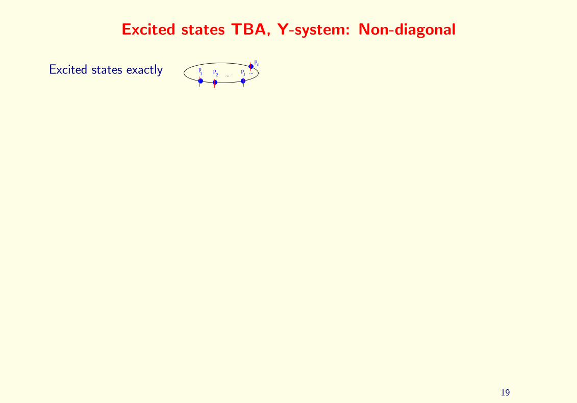
Excited states TBA, Y-system: Non-diagonal
Excited states exactlyn
1 2 j... ...p p p
p
19
Excited states TBA, Y-system: Non-diagonal
Excited states exactlyn
1 2 j... ...p p p
p
L
E
0
2m
m
S−
mat
rix
Bethe−YangLuscherCFT

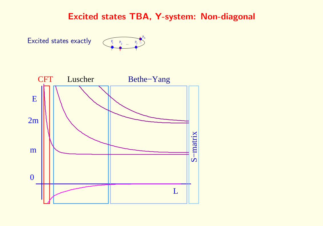
Excited states TBA, Y-system: Non-diagonal
Excited states exactlyn
1 2 j... ...p p p
p
L
E
0
2m
m
S−
mat
rix
Bethe−YangLuscherCFT

Excited states TBA, Y-system: Non-diagonal
Excited states exactlyn
1 2 j... ...p p p
p
L
E
0
2m
m
S−
mat
rix
Bethe−YangLuscherCFT
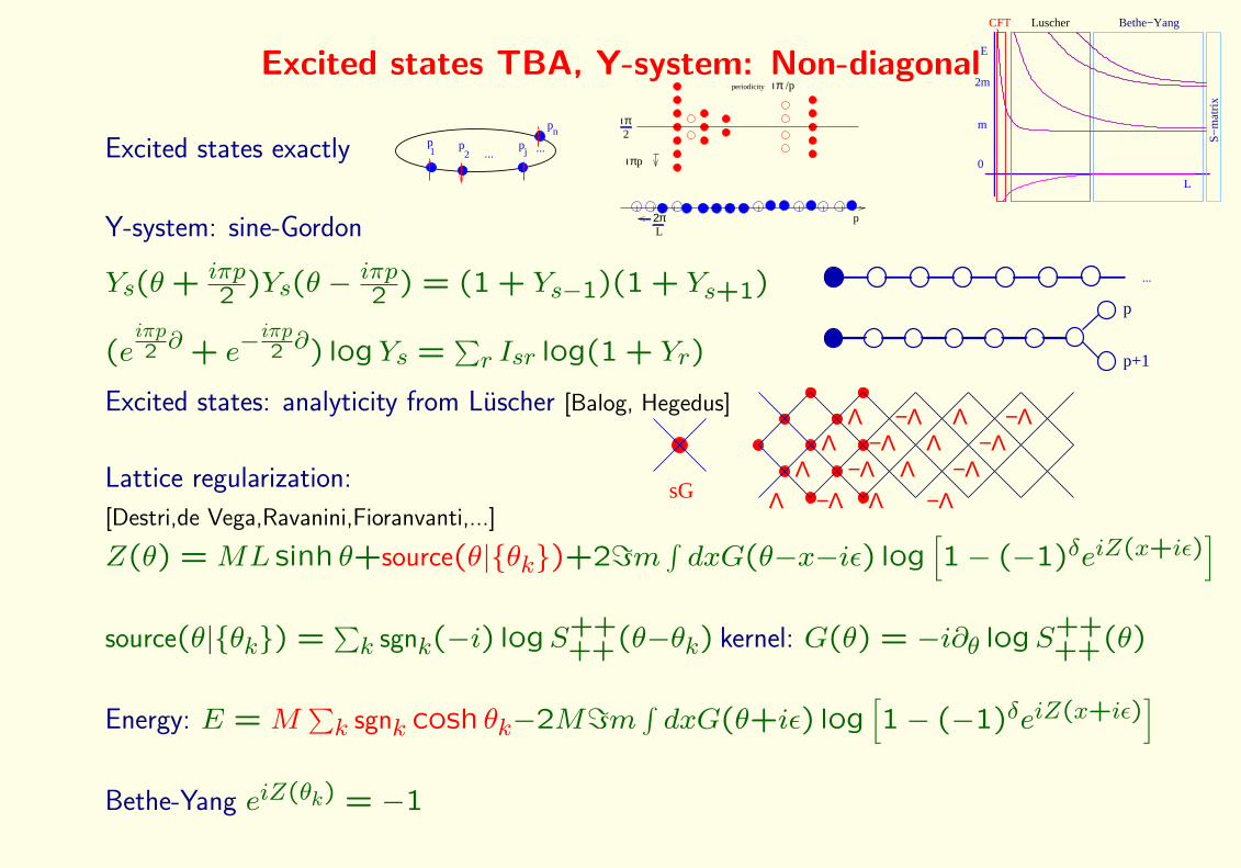
Y-system: sine-Gordon p2πL
ιπ2
ιπp
periodicity ιπ /p
Ys(θ + iπp2 )Ys(θ − iπp
2 ) = (1 + Ys−1)(1 + Ys+1)
(eiπp2 ∂ + e−
iπp2 ∂) logYs =
∑r Isr log(1 + Yr)
...
p
p+1

Excited states TBA, Y-system: Non-diagonal
Excited states exactlyn
1 2 j... ...p p p
p
L
E
0
2m
m
S−
mat
rix
Bethe−YangLuscherCFT
Y-system: sine-Gordon p2πL
ιπ2
ιπp
periodicity ιπ /p
Ys(θ + iπp2 )Ys(θ − iπp
2 ) = (1 + Ys−1)(1 + Ys+1)
(eiπp2 ∂ + e−
iπp2 ∂) logYs =
∑r Isr log(1 + Yr)
...
p
p+1
Excited states: analyticity from Luscher [Balog, Hegedus]
Lattice regularization:
[Destri,de Vega,Ravanini,Fioranvanti,...] ΛΛ
ΛΛ
ΛΛ
ΛΛ
−Λ−Λ
−Λ−Λ
−Λ−Λ
−Λ−Λ
sG
Excited states TBA, Y-system: Non-diagonal
Excited states exactlyn
1 2 j... ...p p p
p
L
E
0
2m
m
S−
mat
rix
Bethe−YangLuscherCFT
Y-system: sine-Gordon p2πL
ιπ2
ιπp
periodicity ιπ /p
Ys(θ + iπp2 )Ys(θ − iπp
2 ) = (1 + Ys−1)(1 + Ys+1)
(eiπp2 ∂ + e−
iπp2 ∂) logYs =
∑r Isr log(1 + Yr)
...
p
p+1
Excited states: analyticity from Luscher [Balog, Hegedus]
Lattice regularization:
[Destri,de Vega,Ravanini,Fioranvanti,...]Λ
ΛΛ
Λ
ΛΛ
ΛΛ
−Λ−Λ
−Λ−Λ
−Λ−Λ
−Λ−Λ
sG
Z(θ) = ML sinh θ+source(θ|{θk})+2=m∫dxG(θ−x−iε) log
[1− (−1)δeiZ(x+iε)
]source(θ|{θk}) =
∑k sgnk(−i) logS++
++(θ−θk) kernel: G(θ) = −i∂θ logS++++(θ)
Energy: E = M∑k sgnk cosh θk−2M=m
∫dxG(θ+iε) log
[1− (−1)δeiZ(x+iε)
]Bethe-Yang eiZ(θk) = −1
Excited states TBA, Y-system: AdS g
Classical string theory
Semiclassical string theory
J
1 loop perturbative gauge theory
+ string loop corrections
Nonperturbative gauge theory
Quantum String theory
S −
mat
rix
+ gauge loop corrections
Asy
mpt
otic
Bet
he A
nsat
z
Wra
ppin
g/Lu
sche
r co
rrec
tion
Excited states exactlyn
1 2 j... ...p p p
p
20

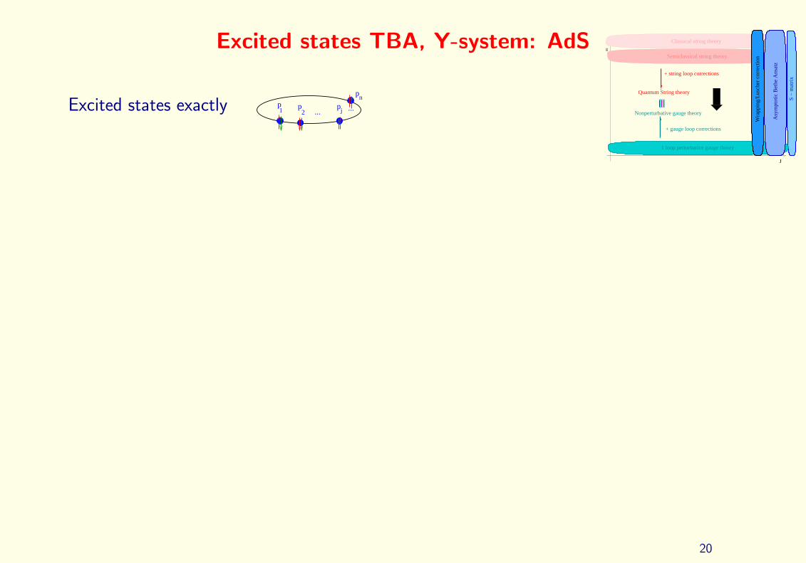
Excited states TBA, Y-system: AdS g
Classical string theory
Semiclassical string theory
J
1 loop perturbative gauge theory
+ string loop corrections
Nonperturbative gauge theory
Quantum String theory
S −
mat
rix
+ gauge loop corrections
Asy
mpt
otic
Bet
he A
nsat
z
Wra
ppin
g/Lu
sche
r co
rrec
tion
Excited states exactlyn
1 2 j... ...p p p
p
Y-system: AdS [Gromov,Kazakov,Viera]
i
no periodicity
Ya,s(θ+ i2)Ya,s(θ− i
2)Ya+1,sYa−1,s
=(1+Ya,s−1)(1+Ya,s+1)(1+Ya+1,s)(1+Ya−1,s)
Excited states: analyticity from Luscher [Gromov,Kazakov]
Assumption on analytical structure→excited state TBA [Gromov,Kazakov,Kozak,Viera]
NO µ terms!
NEEDs ANALYTICAL CHECKS: 5 loop Konishi
Cannot be the final answer→ Lattice regularization: ?

Conclusion
21

Conclusion
g
Classical string theory
Semiclassical string theory
J
1 loop perturbative gauge theory
+ string loop corrections
Nonperturbative gauge theory
Quantum String theory
S −
mat
rix
+ gauge loop corrections
Asy
mpt
otic
Bet
he A
nsat
z
Wra
ppin
g/Lu
sche
r co
rrec
tion

Conclusion
g
Classical string theory
Semiclassical string theory
J
1 loop perturbative gauge theory
+ string loop corrections
Nonperturbative gauge theory
Quantum String theory
S −
mat
rix
+ gauge loop corrections
Asy
mpt
otic
Bet
he A
nsat
z
Wra
ppin
g/Lu
sche
r co
rrec
tion

Conclusion
g
Classical string theory
Semiclassical string theory
J
1 loop perturbative gauge theory
+ string loop corrections
Nonperturbative gauge theory
Quantum String theory
S −
mat
rix
+ gauge loop corrections
Asy
mpt
otic
Bet
he A
nsat
z
Wra
ppin
g/Lu
sche
r co
rrec
tion
S-matrix = scalar . Matrix
physical sheet, explanation of all the poles
Excited states = analiticity . Y-system
Analytical structure of all excited states
lattice?
