fir filter designhcso/ee5410_10.pdf · existence of optimality theorem for fir filter design ....

H. C. So Semester A 2019-2020

FIR Filter Design Chapter Intended Learning Outcomes: (i) Understanding of the characteristics of linear-phase finite impulse response (FIR) filters (ii) Ability to design linear-phase FIR filters according to predefined specifications using the window and frequency sampling methods


Steps in Digital Filter Design 1. Specification Determination

The first step is to obtain the filter specifications or requirements which are determined by the applications. Suppose we have observations where is the signal of interest and is the additive noise. The only has low-frequency components such that for

while is of wideband such that for the whole frequency range. If our task is to find from , we can use a lowpass filter with cutoff frequency of to obtain a noise-reduced version of .


Fig.10.1: Spectra of signal and noise

The filter specification can be described by discrete-time Fourier transform (DTFT) : (10.1)

which specifies both the magnitude and phase


Fig.10.2: Ideal lowpass filter

unity gain for the whole range of

complete suppression for

step change in frequency response at


passband transition stopband

Fig.10.3: Practical

passband corresponds to where is the

passband frequency and is the passband ripple or tolerance which is the maximum allowable deviation from unity in this band


stopband corresponds to where is the stopband frequency and is the stopband ripple or tolerance which is the maximum allowable deviation from zero in this band

transition band corresponds to where there are no restrictions on in this band

2. Filter Response Calculation

We then use digital signal processing techniques to obtain a filter description in terms of transfer function or impulse response that fulfills the given specifications 3. Implementation

When or are known, the filter can then be realized in hardware or software according to a given structure


Advantages of FIR Filter

Transfer function of a causal FIR filter with length is:

(10.2)

where is the finite-duration impulse response

Phase response can be exactly linear which results in computation reduction and zero phase distortion. Note that when there is phase distortion, different frequency components of a signal will undergo different delays in the filtering process

It is always stable because for finite

Less sensitive to finite word-length effects


Efficient implementation via digital signal processors with multiply-and-add (MAC) instruction

Existence of optimality theorem for FIR filter design Linear-Phase FIR Filter

The phase response of a linear-phase filter is a linear function of the frequency :

(10.3)

where equals 0 or and is a constant which is function of the filter length.

Note that (10.3) is slightly different from that in previous chapters where the phase response complements with the magnitude response .


Here, the phase response is related to by

(10.4)

where is real and is called the amplitude response. Comparing

(10.5) where is nonnegative, we see that when is positive, the phase responses in (10.4) and (10.5) are identical but there is a phase difference of for a negative

.


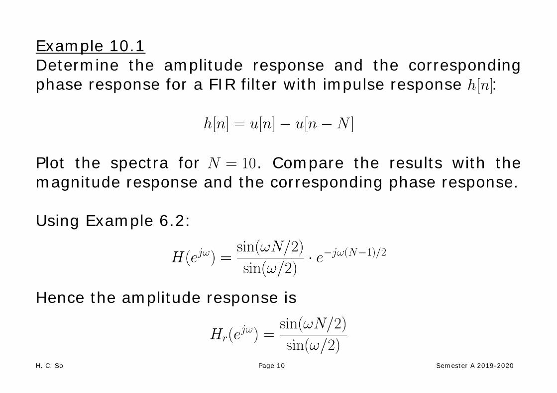
Example 10.1 Determine the amplitude response and the corresponding phase response for a FIR filter with impulse response :

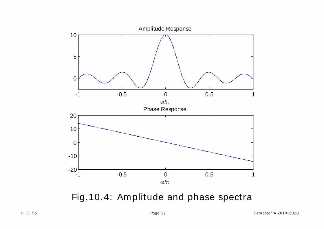
Plot the spectra for . Compare the results with the magnitude response and the corresponding phase response. Using Example 6.2:

Hence the amplitude response is


and the corresponding phase response is

On the other hand, the magnitude response and the corresponding phase response are:

and

The MATLAB program is provided as ex10_1.m.


Fig.10.4: Amplitude and phase spectra

-1 -0.5 0 0.5 1

0

5

10Amplitude Response

ω/π

-1 -0.5 0 0.5 1-20

-10

0

10

20Phase Response

ω/π


Fig.10.5: Magnitude and phase spectra

-1 -0.5 0 0.5 1

0

5

10Magnitude Response

ω/π

-1 -0.5 0 0.5 1-20

-10

0

10

20Phase Response

ω/π


For a causal linear-phase FIR filter, the impulse response is either symmetric or anti-symmetric:

(10.6) or

(10.7)

For example, when is even in (10.7):

, ,

(10.8) How many multipliers and additions are needed?


Example 10.2 Draw the block diagram using the direct form with minimum number of multiplications for the FIR filter whose impulse response is:

Following (10.8), we obtain:

The number of multiplications is reduced from to while the number of additions remains unchanged, which is 4.


Fig.10.6: Block diagram for symmetric impulse response


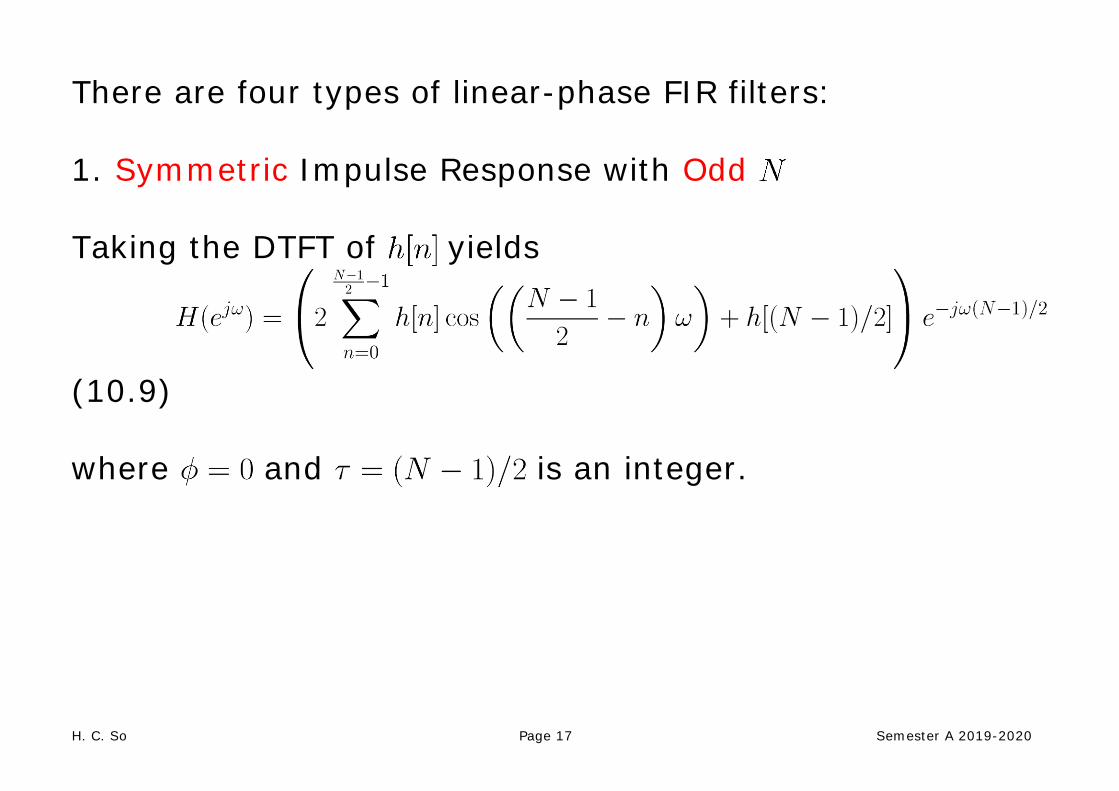
There are four types of linear-phase FIR filters: 1. Symmetric Impulse Response with Odd Taking the DTFT of yields

(10.9) where and is an integer.


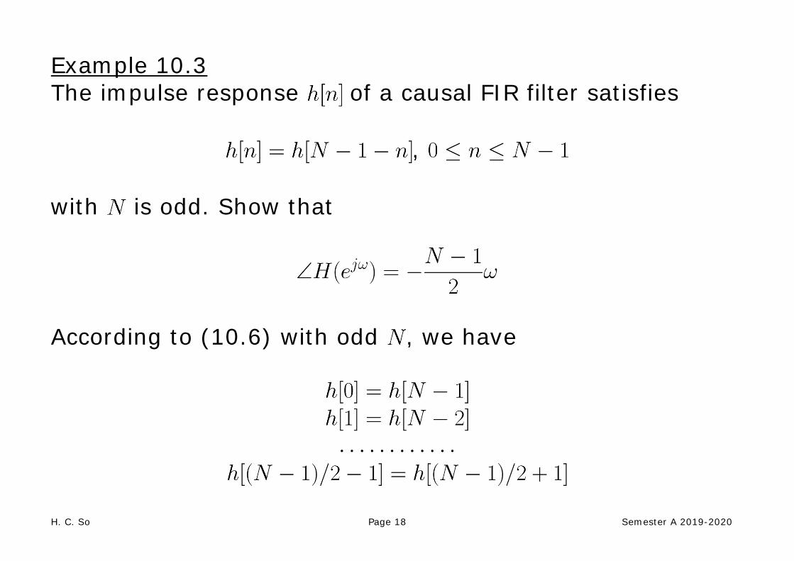
Example 10.3 The impulse response of a causal FIR filter satisfies

, with is odd. Show that

According to (10.6) with odd , we have


Hence

which validates (10.9) with .


2. Symmetric Impulse Response with Even The DTFT of is:

(10.10)

where and is not an integer. 3. Anti-symmetric Impulse Response with Odd The DTFT of is:

(10.11)


where and is an integer Note that due to anti-symmetric property 4. Anti-symmetric Impulse Response with Even Taking the DTFT of yields:

(10.12)

where and is not an integer.


Example 10.4 Consider an input sequence of length 400 such that

for and , and it is a sinusoid with frequencies and for and , respectively. Examine the filter output with the following two FIR systems: (a) with (b) with Are they linear phase filters? The MATLAB program for this example is provided as ex10_4.m.


Fig.10.7: Pulsed sinusoid with two frequencies

0 50 100 150 200 250 300 350 400-1

-0.8

-0.6

-0.4

-0.2

0

0.2

0.4

0.6

0.8

1

n

x[n]


Fig.10.8: Filter output with nonlinear-phase filter

0 50 100 150 200 250 300 350 400-2

-1.5

-1

-0.5

0

0.5

1

1.5

2

n

x[n]y[n]


Fig.10.9: Filter output with linear-phase filter

0 50 100 150 200 250 300 350 400-2

-1.5

-1

-0.5

0

0.5

1

1.5

2

n

x[n]y[n]


Example 10.5 The impulse response of a causal linear-phase FIR is:

where . Determine . Plot the amplitude and phase responses and then deduce the function of the filter. Find the expected filter output when passing an input sequence of the form through the filter. As is odd and is anti-symmetric, we apply (10.11):


Fig.10.10: Amplitude and phase responses of differentiator

-1 -0.5 0 0.5 1-4

-2

0

2

4Amplitude Response

ω/π

-1 -0.5 0 0.5 1-20

-10

0

10

20Phase Response

ω/π


The amplitude response can be approximated as:

According to the time-shifting property, the DTFT of with a time advance of 5 samples is then:

This means that the causal FIR filter has a frequency response approximately equals with a delay of 5 samples.


The system with frequency response is known as the differentiator. Recall:

Differentiating both sides with respect to yields:


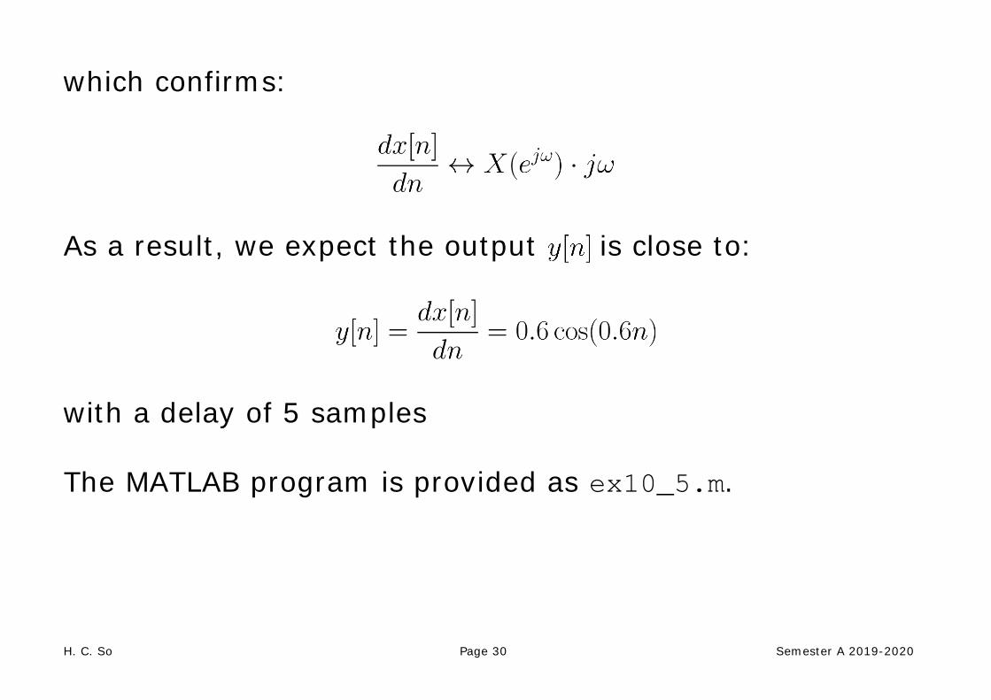
which confirms:

As a result, we expect the output is close to:

with a delay of 5 samples The MATLAB program is provided as ex10_5.m.


Fig.10.11: Differentiator output with sinusoidal input

0 10 20 30 40 50-1

-0.8

-0.6

-0.4

-0.2

0

0.2

0.4

0.6

0.8

1

n

x[n]y[n]


Window Method Based on directly approximating the desired frequency response

Ideal impulse response is calculated from inverse DTFT:

(10.13)

What are the problems in using (10.13)?


Example 10.6 Determine the impulse response of an ideal lowpass filter with a cutoff frequency of . The DTFT of the filter is:

Using Example 6.3, is:

where

Ideal filter is noncausal and its impulse response is of infinite length


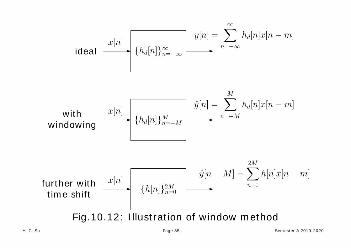
The basic idea of window method is to truncate to obtain a linear-phase and causal FIR filter via 2 steps:

Windowing

Extract a finite set of with positive and negative time indexes because the impulse response is generally symmetric or anti-symmetric around , say, { ,

} corresponding to a length of

Filter response is linear phase but is only an approximation of due to the coefficient truncation

Time Shifting

Delay by samples to obtain with to achieve causality

Filter output is received after a delay of samples


ideal

with windowing

further with time shift

Fig.10.12: Illustration of window method


Example 10.7 Use the window method to design a linear-phase and causal FIR system with 7 coefficients to approximate an ideal lowpass filter whose cutoff frequency is . From Example 10.6:

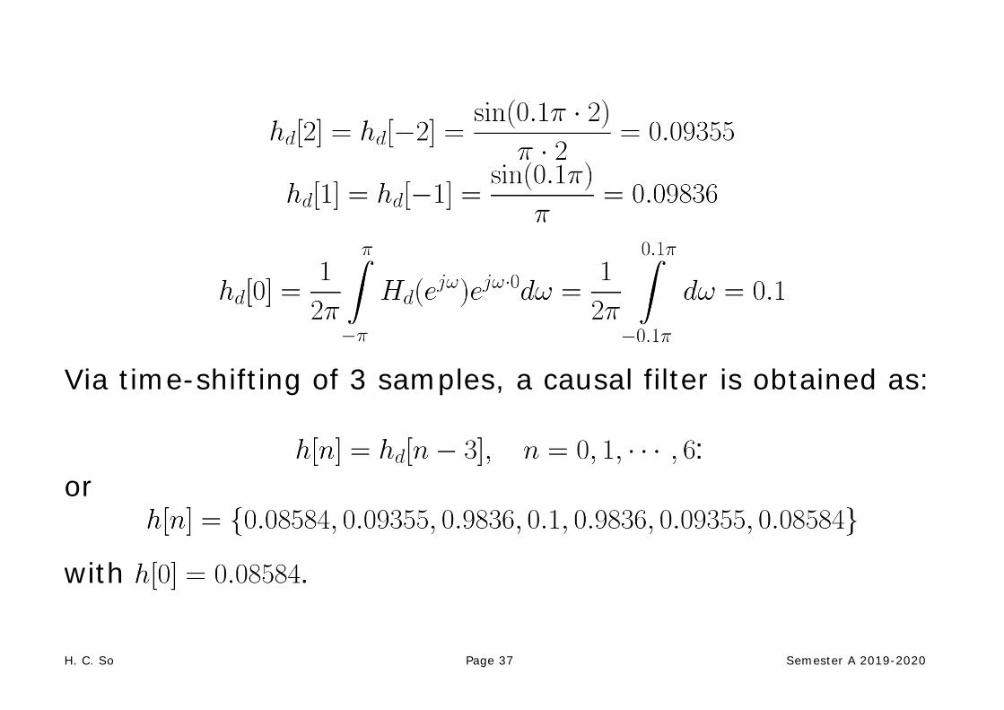
Via windowing, we extract the set of . Notice that is symmetric around at as . Their values are calculated as:


Via time-shifting of 3 samples, a causal filter is obtained as:

: or

with .


Fig.10.13: Magnitude response of lowpass filter with

0 0.2 0.4 0.6 0.8 10

0.1

0.2

0.3

0.4

0.5

0.6

0.7Magnitude Response

ω/π


Note that we can use the MATLAB command fir1(6,0.1,boxcar(7),'noscale') to produce Alternatively, we can first perform the time shifting prior to windowing As there should be a phase of where in the practical filter, we modify the desired frequency response as:

Note that multiplying in the frequency domain corresponds to a time shift of in the time domain.


The corresponding impulse response is

As the filter length is , we then perform windowing on

Substituting and yields the same FIR impulse response. Note that we can base on this approach to determine even when is an even integer


The truncation operation can be considered as multiplying by a rectangular window function:

That is,

Generally speaking, is not restricted to be rectangular and it can be any symmetric function so that the resultant filter is linear phase


Example 10.8 Use the window method to design a linear-phase and causal FIR filter of length 101 such that the sampled version of a continuous-time sinusoid with frequency of 80 Hz can pass through it with negligible attenuation while the sampled signal corresponds to a tone of frequency 120 Hz will be suppressed. The sampling frequency is 1000 Hz. Let the continuous-time sinusoids be

From (4.1), the corresponding discrete-time versions with sampling interval of s are


which gives:

and

The frequencies are and in discrete-time domain. In order to suppress while keeping , we can use a lowpass filter with cutoff frequency of , which is simply the average of the two discrete frequencies. Using Example 10.7 with and , the required filter impulse response is:


Fig.10.14: Impulse response of lowpass filter with

0 20 40 60 80 100-0.05

0

0.05

0.1

0.15

0.2

n

h[n]


Fig.10.15: Magnitude response of lowpass filter with

0 0.2 0.4 0.6 0.8 10

0.2

0.4

0.6

0.8

1

Magnitude Response

ω/π


Fig.10.16: Discrete-time tone with frequency

100 120 140 160 180 200-1

-0.8

-0.6

-0.4

-0.2

0

0.2

0.4

0.6

0.8

1

n

s

1[n]


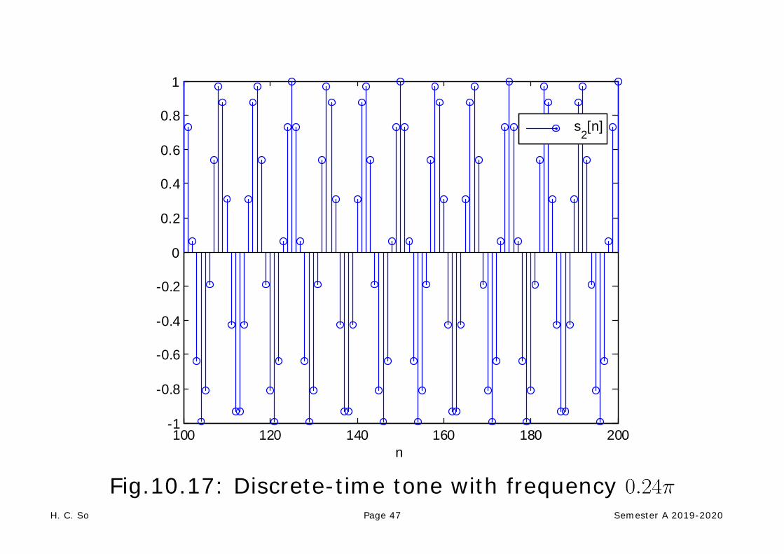
Fig.10.17: Discrete-time tone with frequency

100 120 140 160 180 200-1

-0.8

-0.6

-0.4

-0.2

0

0.2

0.4

0.6

0.8

1

n

s2[n]


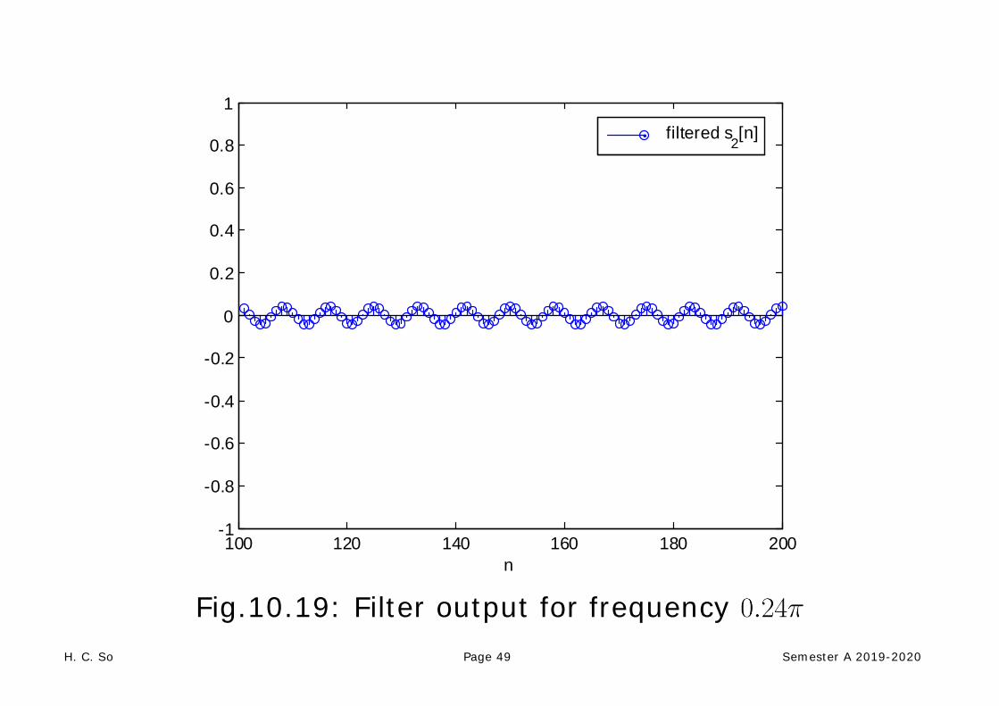
Fig.10.18: Filter output for frequency

100 120 140 160 180 200-1

-0.8

-0.6

-0.4

-0.2

0

0.2

0.4

0.6

0.8

1

n

filtered s1[n]


Fig.10.19: Filter output for frequency

100 120 140 160 180 200-1

-0.8

-0.6

-0.4

-0.2

0

0.2

0.4

0.6

0.8

1

n

filtered s2[n]


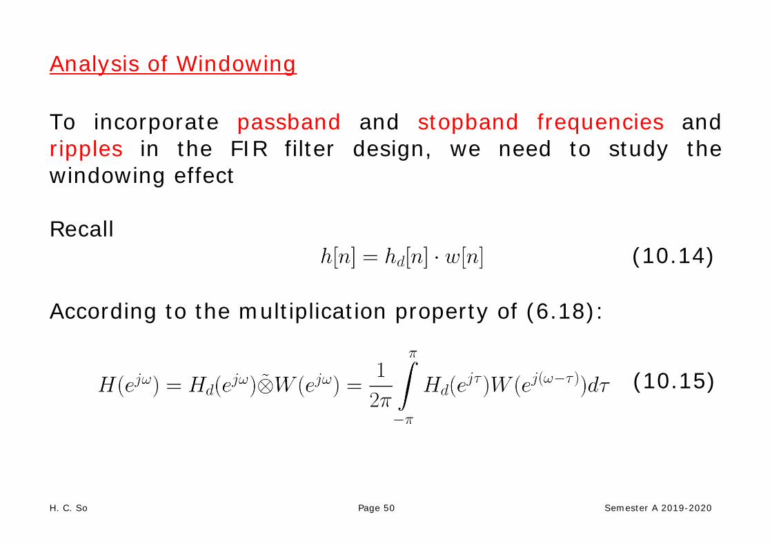
Analysis of Windowing To incorporate passband and stopband frequencies and ripples in the FIR filter design, we need to study the windowing effect Recall

(10.14) According to the multiplication property of (6.18):

(10.15)


Side lobes

Main lobewidth

Ripples

Transition

Fig.10.20: Illustration of


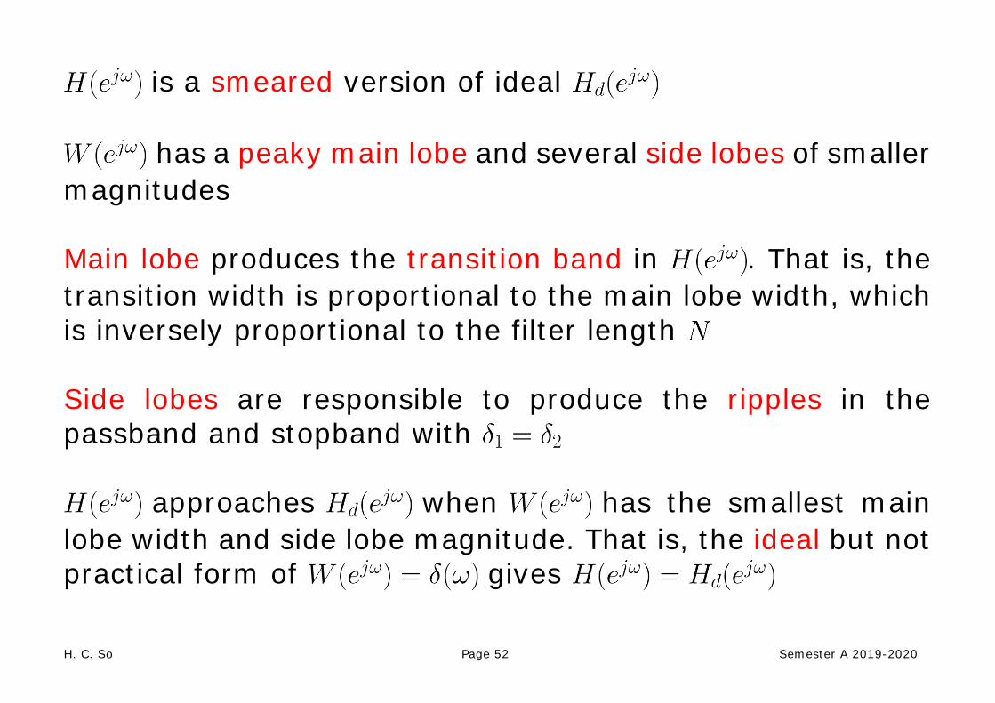
is a smeared version of ideal

has a peaky main lobe and several side lobes of smaller magnitudes Main lobe produces the transition band in . That is, the transition width is proportional to the main lobe width, which is inversely proportional to the filter length Side lobes are responsible to produce the ripples in the passband and stopband with

approaches when has the smallest main lobe width and side lobe magnitude. That is, the ideal but not practical form of gives


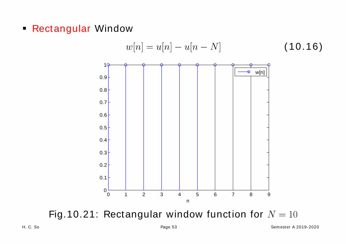
Rectangular Window

(10.16)

Fig.10.21: Rectangular window function for

0 1 2 3 4 5 6 7 8 90

0.1

0.2

0.3

0.4

0.5

0.6

0.7

0.8

0.9

1

n

w[n]


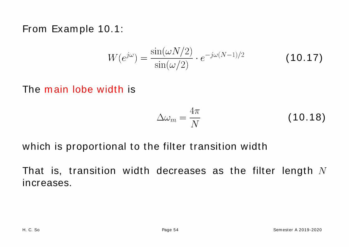
From Example 10.1:

(10.17)

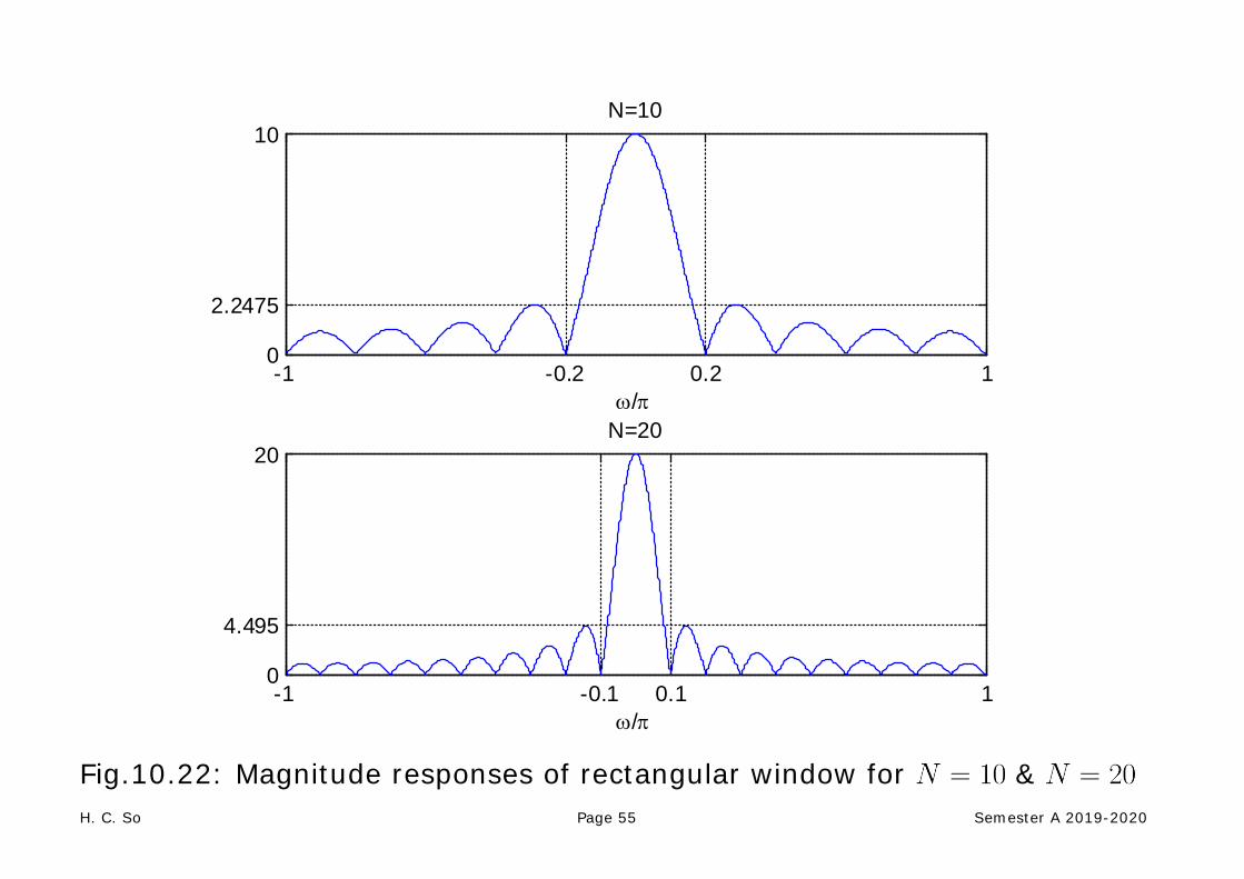
The main lobe width is

(10.18)

which is proportional to the filter transition width That is, transition width decreases as the filter length increases.


Fig.10.22: Magnitude responses of rectangular window for &

-1 -0.2 0.2 10

2.2475

10N=10

ω/π

-1 -0.1 0.1 10

4.495

20N=20

ω/π


Relative peak side lobe, , is the ratio of the peak side lobe height to main lobe height in dB:

(10.19)

A larger implies ripples with bigger magnitudes

As increases, widths of the main lobe and all side lobes decrease but their areas remain unchanged, meaning that the ripples cannot be reduced. This is known as Gibbs phenomenon due to sudden change in transition from 0 to 1 and 1 to 0. This can be removed by tapering the window smoothly to zero at each end. However, the heights of the side lobes can be diminished but at the expense of wider main lobe and hence a wider transition.


Bartlett Window

(10.20)

Fig.10.23: Bartlett window function for

0 1 2 3 4 5 6 7 8 90

0.1

0.2

0.3

0.4

0.5

0.6

0.7

0.8

0.9

n

w[n]


Hanning Window

(10.21)

Fig.10.24: Hanning window function for

0 1 2 3 4 5 6 7 8 90

0.1

0.2

0.3

0.4

0.5

0.6

0.7

0.8

0.9

1

n

w[n]


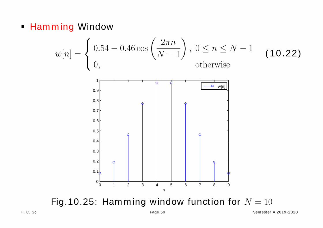
Hamming Window

(10.22)

Fig.10.25: Hamming window function for

0 1 2 3 4 5 6 7 8 90

0.1

0.2

0.3

0.4

0.5

0.6

0.7

0.8

0.9

1

n

w[n]


Blackman Window

(10.23)

Fig.10.26: Blackman window function for

0 1 2 3 4 5 6 7 8 90

0.1

0.2

0.3

0.4

0.5

0.6

0.7

0.8

0.9

1

n

w[n]


Note that by using terms for a filter length of and then discarding the end points, we can avoid zero coefficients at both ends for Bartlett, Hanning and Blackman windows.

Window (dB) Rectangular Bartlett Hanning Hamming Blackman

Table 10.1: Characteristics of window functions As a result, there is a tradeoff between transition and ripple


Example 10.9 Use the window method to design a linear-phase and causal FIR system to approximate an ideal lowpass filter whose cutoff frequency is . Try the rectangular and Bartlett window functions with filter lengths of 7, 21, 61 and 101, to investigate the frequency magnitude responses. Using Example 10.7, with the rectangular window is:

with equals 7, 21, 61 and 101 and .

Multiplying by (10.20) yields the corresponding filter coefficients for the Bartlett window.



Fig.10.27: Magnitude responses with rectangular window at different

0 0.5 10

0.5

1

N=7

ω/π0 0.5 1

0

0.5

1

N=21

ω/π

0 0.5 10

0.5

1

N=61

ω/π0 0.5 1

0

0.5

1

N=101

ω/π


Fig.10.28: Magnitude responses with Bartlett window at different

0 0.5 10

0.5

1

N=7

ω/π0 0.5 1

0

0.5

1

N=21

ω/π

0 0.5 10

0.5

1

N=61

ω/π0 0.5 1

0

0.5

1

N=101

ω/π


Example 10.10 Use the window method to find the impulse response of a linear-phase and causal FIR filter which approximates an ideal lowpass filter whose cutoff frequency is . It is required that the filter is of fourth-order and Bartlett window is employed. A fourth-order filter implies a filter length of . Using Example 10.7 with and :

To avoid zero coefficients, we set in (10.20) and extract the middle 5 values to yield with

.


As a result

with

is:

The MATLAB command fir1(4,0.25,triang(5),'noscale') can also produce . Note that if we use in (10.20), with . The resultant impulse response will be

with , indicating that the effective length is only 3


In window method, the ripple is:

And the transition width is:

with or

and They are determined from in (10.15), which is not straightforward for computation Nevertheless, by noting that (10.15) corresponds to one of the forms in (10.9)-(10.12), is easily obtained by extracting the amplitude


Step 1: Find

Step 2: Find

Step 3: Find

Step 4: Find

Fig.10.29: Steps to find passband and stopband ripples and frequencies


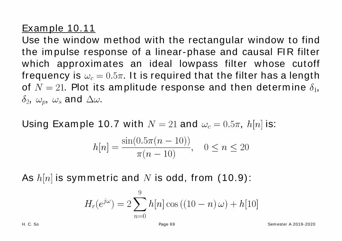
Example 10.11 Use the window method with the rectangular window to find the impulse response of a linear-phase and causal FIR filter which approximates an ideal lowpass filter whose cutoff frequency is . It is required that the filter has a length of . Plot its amplitude response and then determine ,

, , and . Using Example 10.7 with and , is:

As is symmetric and is odd, from (10.9):


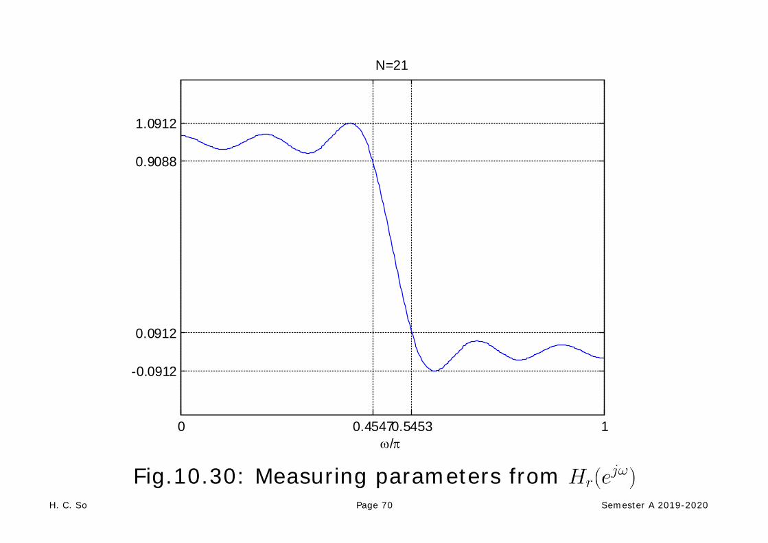
Fig.10.30: Measuring parameters from

0 0.45470.5453 1

-0.0912

0.0912

0.9088

1.0912

N=21

ω/π


We see that

Peak approximation error, , which is the ripple in dB, is:

Furthermore

and

which gives

with



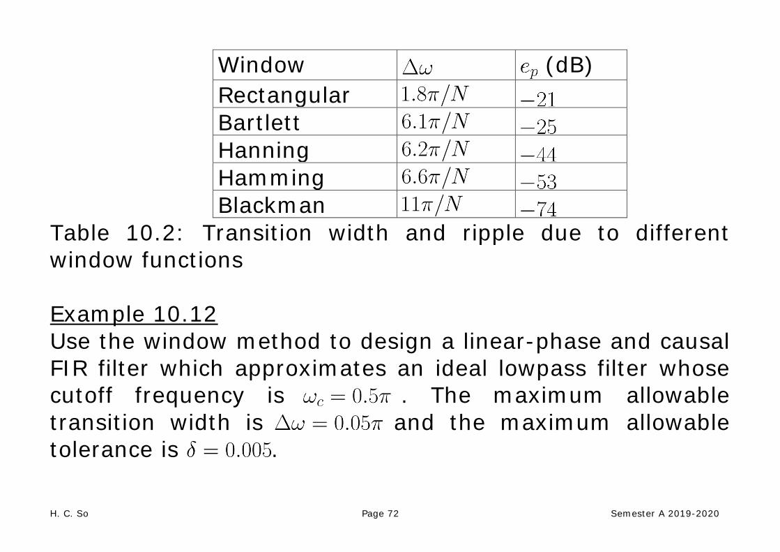
Window (dB) Rectangular Bartlett Hanning Hamming Blackman

Table 10.2: Transition width and ripple due to different window functions Example 10.12 Use the window method to design a linear-phase and causal FIR filter which approximates an ideal lowpass filter whose cutoff frequency is . The maximum allowable transition width is and the maximum allowable tolerance is .


The ripple of corresponds to:

From Table 10.2, Hamming and Blackman windows are the two candidates which can meet the ripple requirement We choose the former because it involves a shorter filter length. The required length for the Hamming window is:

Using Example 10.7 with and , the filter impulse response is:


Fig.10.31: Magnitude response with Hamming window

0 0.5 1

-53-46

0

N=132

ω/π


Fig.10.32: Amplitude response with Hamming window

0 0.2 0.4 0.6 0.8 10

0.1

0.2

0.3

0.4

0.5

0.6

0.7

0.8

0.9

1N=132

ω/π


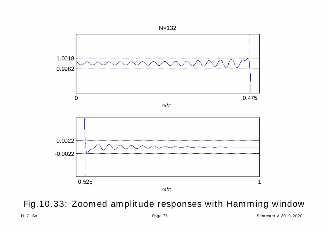
Fig.10.33: Zoomed amplitude responses with Hamming window

0 0.475

0.9982

1.0018

N=132

ω/π

0.525 1

-0.0022

0.0022

ω/π


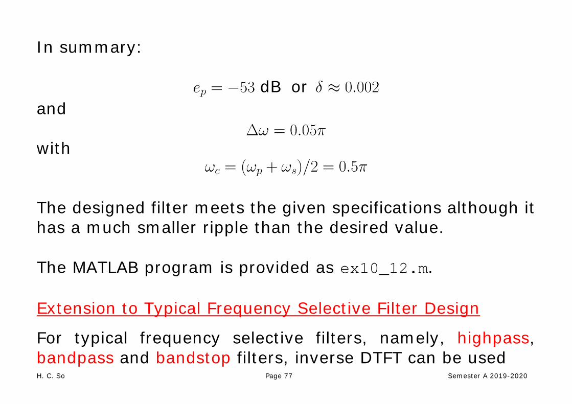
In summary:

dB or and

with

The designed filter meets the given specifications although it has a much smaller ripple than the desired value. The MATLAB program is provided as ex10_12.m. Extension to Typical Frequency Selective Filter Design

For typical frequency selective filters, namely, highpass, bandpass and bandstop filters, inverse DTFT can be used


lowpass

bandpass

highpass

bandstop

Fig.10.34: Typical frequency-selective filters


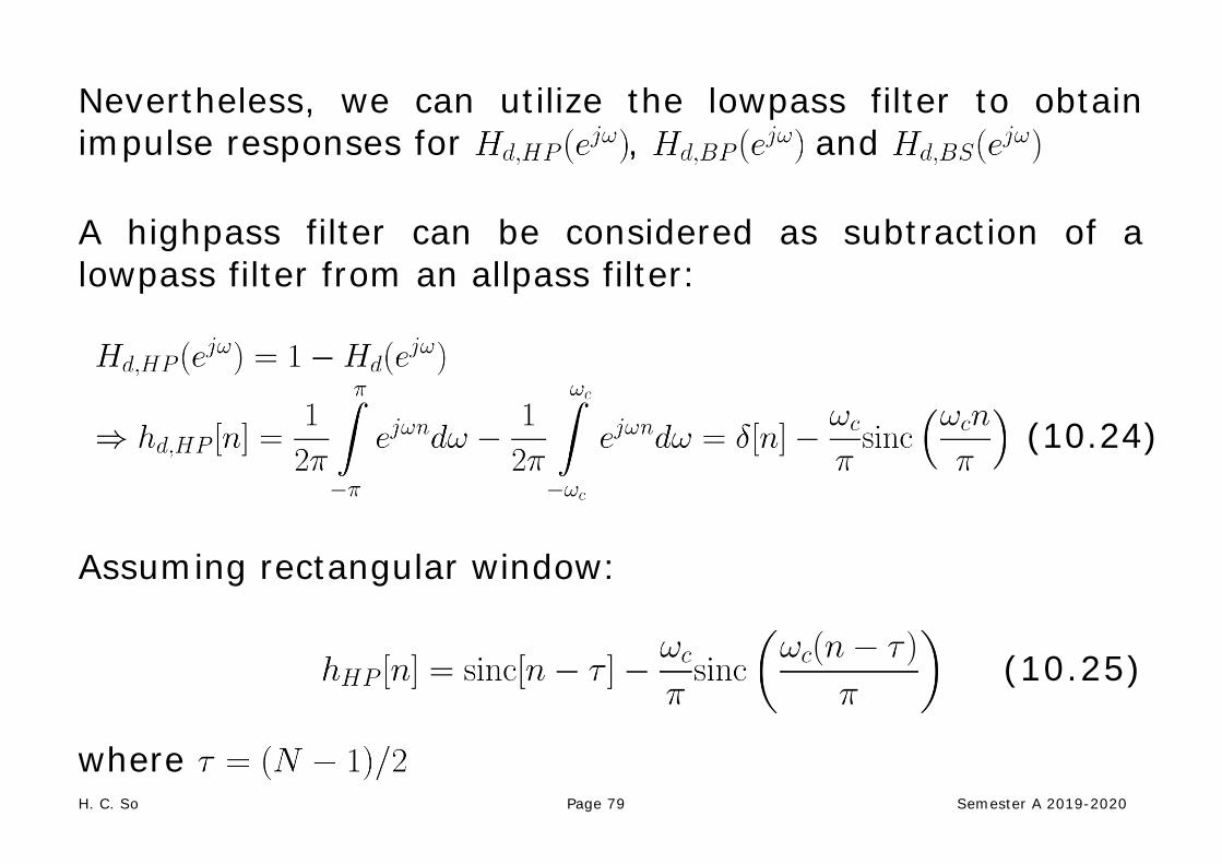
Nevertheless, we can utilize the lowpass filter to obtain impulse responses for , and A highpass filter can be considered as subtraction of a lowpass filter from an allpass filter:

(10.24)

Assuming rectangular window:

(10.25)

where


Example 10.13 Use the window method with the rectangular window to find the impulse response of a linear-phase and causal FIR filter which approximates an ideal highpass filter whose cutoff frequency is . It is required that the filter has a length of . According to (10.25) with and :

Note that we can also use the MATLAB command fir1(20,0.5,'high',boxcar(21),'noscale') to get the same result The MATLAB program is provided as ex10_13.m.


Fig.10.35: Impulse response of highpass filter with

0 5 10 15 20-0.4

-0.3

-0.2

-0.1

0

0.1

0.2

0.3

0.4

0.5

n

h[n]


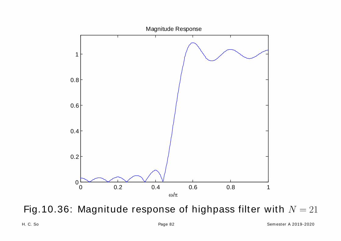
Fig.10.36: Magnitude response of highpass filter with

0 0.2 0.4 0.6 0.8 10

0.2

0.4

0.6

0.8

1

Magnitude Response

ω/π


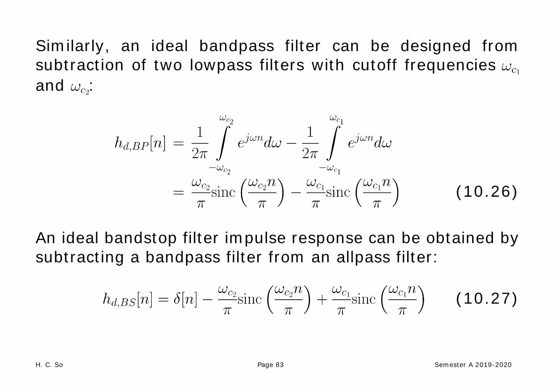
Similarly, an ideal bandpass filter can be designed from subtraction of two lowpass filters with cutoff frequencies and :

(10.26)

An ideal bandstop filter impulse response can be obtained by subtracting a bandpass filter from an allpass filter:

(10.27)


Kaiser Window A problem in typical window functions is that we cannot control the ripple Kaiser window can control both and in a nearly optimal manner and it has the form of:

(10.28)

where is the modified zero-order Bessel function. Apart from , there is which is responsible for the window shape


That is, by properly choosing and , the design specifications in terms of and can be precisely met

is computed as:

(10.29)

where is the peak approximation error and rounds up to the nearest integer is determined from:

(10.30)


Example 10.14 Use the window method with the Kaiser window to design a linear-phase and causal FIR filter which approximates an ideal lowpass filter whose cutoff frequency is . The maximum allowable transition width is and the maximum allowable tolerance is . Since

and , we then have:

and


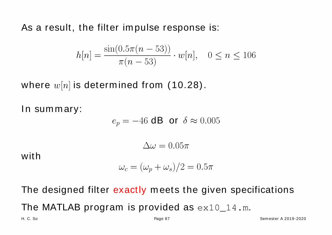
As a result, the filter impulse response is:

where is determined from (10.28). In summary:

dB or

with

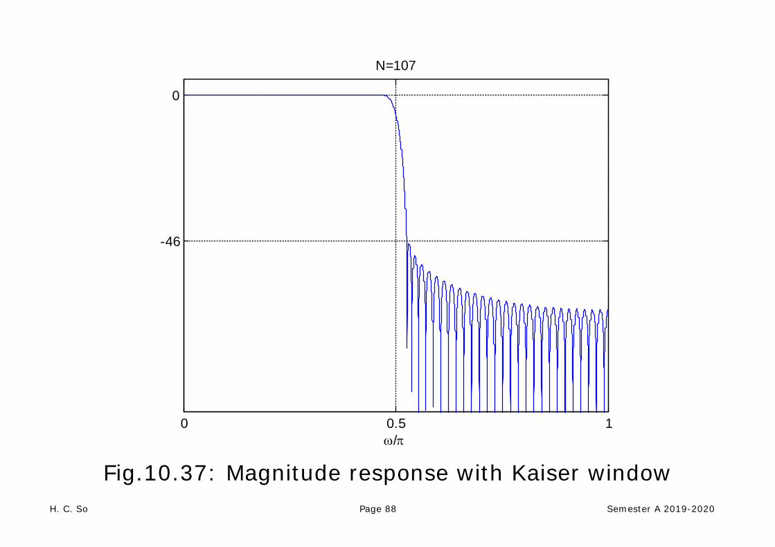
The designed filter exactly meets the given specifications



Fig.10.37: Magnitude response with Kaiser window

0 0.5 1

-46

0

N=107

ω/π


Fig.10.38: Amplitude response with Kaiser window

0 0.2 0.4 0.6 0.8 10

0.1

0.2

0.3

0.4

0.5

0.6

0.7

0.8

0.9

1N=107

ω/π


Fig.10.39: Zoomed amplitude responses with Kaiser window

0 0.475

0.9954

1.0046

N=107

ω/π

0.525 1

-0.0046

0.0046

ω/π


Frequency Sampling Method The basic idea is to utilize the discrete Fourier transform (DFT), which corresponds to samples of the desired frequency response , to produce

Recall: (10.31)

is equal to sampled at distinct frequencies between

with a uniform frequency spacing of

A causal and linear-phase filter is designed with 2 steps:

Extract uniformly-spaced samples from in the frequency range of

Compute by taking the inverse DFT of :


(10.32)

Taking transform of :

(10.33)


The filter frequency response is then:

(10.34)

From (10.33) and (7.7) together with (10.31):

(10.35) It is simple as only uniformly-spaced samples of the desired frequency response or the DFT coefficients are needed At , , equals but we cannot control the values of the remaining frequency points


It lacks flexibility in specifying the passband and stopband cutoff frequencies since placement of “1” & “0” & transition samples is constrained to integer multiples of Example 10.15 Use the frequency sampling method to design a linear-phase and causal FIR filter with a length of to approximate an ideal lowpass filter whose cutoff frequency is . From Example 10.7, the ideal frequency response with linear phase is

where and


We consider the frequency interval of :

Extracting the values of at , :

Taking the inverse DFT:



Fig.10.40: Magnitude response based on frequency sampling

0 0.2 0.4 0.6 0.8 10

0.2

0.4

0.6

0.8

1

1.2Magnitude Response

ω/π


Fig.10.41: Amplitude response based on frequency sampling

0 0.2857 0.5714 0.8571 1.1429 1.4286 1.7143

0

1

Amplitude Response

ω/π


Optimal Equiripple Method The basic idea is to evenly distribute the ripples in both passband and stopband Required filter length will be shorter than that of the

window method where its exactly meets the passband or stopband ripple specification at one frequency and is superior to it at other frequencies in the band

Allow Passband and stopband frequencies can be precisely

specified although and are implicitly implied in the window method


Fig.10.42: Illustration of optimal equiripple lowpass filter

Ripples are uniformly distributed such that reaches its maximum deviations of and more than once


The impulse response of optimal equiripple design is determined from:

(10.36)

where

(10.37) which corresponds to a minmax optimization problem

is the frequency-domain error between the desired and actual responses weighted by

is the weighting function incorporates all specification parameters, namely, , , and , into the design process


For example, in lowpass filter design, has the form of:

(10.38)

When , there is a larger weighting at the stopband. On the other hand, implies a larger weighting at the passband To solve for the minmax problem of (10.36), we can make use of the Parks-McClellan algorithm which requires iterations. The corresponding MATLAB command is firpm where the filter length parameter is also required.


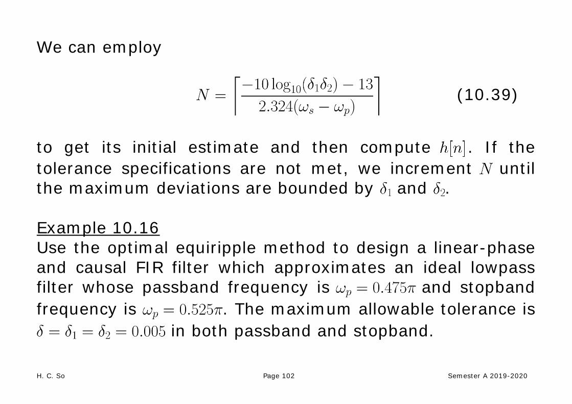
We can employ

(10.39)

to get its initial estimate and then compute . If the tolerance specifications are not met, we increment until the maximum deviations are bounded by and . Example 10.16 Use the optimal equiripple method to design a linear-phase and causal FIR filter which approximates an ideal lowpass filter whose passband frequency is and stopband frequency is . The maximum allowable tolerance is

in both passband and stopband.


According to (10.39), an initial value of is computed as:

Starting with in the Parks-McClellan algorithm, we increment its value until so that the tolerance specifications are met. The MATLAB program is provided as ex10_16.m. In summary:

dB or

,


Fig.10.43: Impulse response of optimal equiripple lowpass filter

0 10 20 30 40 50 60 70 80 90

-0.1

0

0.1

0.2

0.3

0.4

0.5N=96

n

h[n]


Fig.10.44: Magnitude response of optimal equiripple lowpass filter

0 0.5 1

-46

0

Magnitude

ω/π


Fig.10.45: Amplitude response of optimal equiripple lowpass filter

0 0.2 0.4 0.6 0.8 10

0.1

0.2

0.3

0.4

0.5

0.6

0.7

0.8

0.9

1Amplitude Response

ω/π


Fig.10.46: Zoomed amplitude responses of optimal equiripple lowpass filter

0 0.475

0.9952

1.0048

N=96

ω/π

0.525 1

-0.0048

0.0048

ω/π

fir filter designhcso/ee5410_10.pdf · existence of optimality theorem for fir filter design ....

Documents