Firm Internal Network, Environmental Regulation, and Plant Death

Jingbo Cui and GianCarlo Moschini

Working Paper 18-WP 585 October 2018

Center for Agricultural and Rural Development Iowa State University

Ames, Iowa 50011-1070 www.card.iastate.edu

Jingbo Cui is associate professor, School of Economics and Management, Wuhan University, China. E-mail: jbcui2013@gmail.com GianCarlo Moschini is professor and Pioneer Chair in Science and Technology Policy, Department of Economics, Iowa State University, Ames, Iowa. E-mail: moschini@iastate.edu This publication is available online on the CARD website: www.card.iastate.edu. Permission is granted to reproduce this information with appropriate attribution to the author and the Center for Agricultural and Rural Development, Iowa State University, Ames, Iowa 50011-1070.

Iowa State University does not discriminate on the basis of race, color, age, ethnicity, religion, national origin, pregnancy, sexual orientation, gender identity, genetic information, sex, marital status, disability, or status as a U.S. veteran. Inquiries can be directed to the Interim Assistant Director of Equal Opportunity and Compliance, 3280 Beardshear Hall, (515) 294-7612.

0

Firm Internal Network, Environmental Regulation, and Plant Death

Jingbo Cui and GianCarlo Moschini

This version: October 2, 2018

Abstract: This paper examines the role of a firm’s internal network in determining plant shutdown decisions in response to environmental regulations. Using unique plant-level data for U.S. manufacturing industries from 1990 to 2008, we find evidence that, in response to increasingly stringent environmental regulations at the county level, multi-plant firms do exercise their greater flexibility in adjusting production, relative to single-plant firms. Specifically, in regulated counties, the likelihood of a plant shutting down is higher for multi-plant firms. Moreover, we measure the firm internal network effect at the local, neighborhood, and the wider-area levels, as defined by the number of affiliated plants clustered in different regional levels. Their effects on plant closure decisions for dirty subsidiaries vary with the network level. We further decompose the neighborhood network into those in regulated and unregulated neighborhood counties, and examine how these network metrics are associated with closure decisions of dirty plants affiliated with multi-plant firms. The presence of more sibling plants residing in neighboring counties that are free from regulatory controls are associated with a higher closure probability of dirty plants in a regulated county.

Keywords: Agglomeration, Clean Air Act Amendments, Multinationals, Multi-plant firms, Network

effects

JEL Classification: F18, Q56, R11

Jingbo Cui (jbcui2013@gmail.com) is Associate Professor in School of Economics and Management, Wuhan University, China. GianCarlo Moschini (moschini@iastate.edu) is Professor and Pioneer Chair in Science and Technology Policy, Department of Economics and Center for Agricultural and Rural Development, Iowa State University. The authors thank Randy Becker and Ron Shadbegian for comments and suggestions. This paper also benefits from discussions with conference participants at 2017 AERE in Pittsburgh, and 2017 EAERE in Athens. Any remaining errors are on our own.

1

1. Introduction

Environmental regulations have long been of considerable policy interest, and remain controversial.

Supporters of regulatory controls point to significant health benefits associated with reductions in

environmental pollution, while critics blame environmental regulations for productivity drops, job

losses, and relocation of manufacturers. For both sides of the argument, a critical question relates to

how firms respond to environmental regulation. Empirical contributions in this area have sought to

quantify such response (Henderson, 1996; Becker and Henderson, 2000; List et al., 2003b). But the

existing literature has paid little attention to the role of a firm’s plant structure. Because multi-plant

firms may behave differently than single-plant firms, multi-plant firms’ decisions about relocation, in

response to regulatory controls, may impact the effectiveness of environmental regulations. They also

have the potential to play a major role in the dynamics of employment, evolution of regional

economies, and restructuring of industry. This is relevant because multi-plant firms account for a large

share of U.S. manufacturing activities—as noted by Bernard and Jensen (2007), they employ 78% of

the manufacturing workforce and produce 88% of the output. Multi-plant firms are also more likely

to have emission above the critical level that triggers the need for regulatory compliance (Becker and

Henderson, 2000).

In this paper, we follow Bernard and Jensen (2007) by focusing squarely on the probability of

plant death, and investigate a channel that was not investigated in their analysis. Specifically, we study

the impact of environmental regulation on plant death: the extent to which stringent regulation leads

“dirty” plants to exit an industry. In the process, the effects on plant closure of plant attributes, local

agglomeration, and some county characteristics are investigated as well. Second, we examine whether

multi-plant firms are more or less likely to shut down affiliated plants in response to stringent

regulatory controls. Moreover, information on existing plants affiliated with the same headquarter is

used to investigate the role of firms’ internal network. We measure internal network effects at three

different regional levels: local, neighborhood, and the wider area, and we examine how these internal

network effects interact with exposure to environmental regulations. We further decompose the

neighborhood network into those in regulated and unregulated neighboring counties, and examine

how these network measures affect closure decisions of dirty plants (relative to clean ones) affiliated

with multi-plant firms.

The particular empirical focus of this paper on the role of multi-plant firms, and their internal

structure, is motivated by the theoretical ambiguity of how differently multi-plant firms, relative to

2

single-plant firms, may respond to external pressure affecting profitability (Bernard and Jensen, 2007).

In our context, multi-plant firms may exercise their greater flexibility in different ways. The availability

of multiple plants may reduce the closure probability of a given plant because the firm may abate

pollution by reallocating production activities across plants. Alternatively, a multi-plant firm may use

plant shutdown as the margin of adjustment to comply with environmental regulation. The costs of a

plant’s closure are lessened by the ability to shift production activities (and associated jobs) from plants

in regulated areas to plants in unregulated areas. The consequences of plant closure are clearly less

draconian for multi-plant firms—closure does not imply the end of the firm. The options available to

single-plant firms in regulated areas, on the other hand, are more limited.

To carry out the empirical analysis outlined in the foregoing, we compile a unique detailed plant-

level dataset for the U.S. manufacturing sector from 1990 to 2008. To measure plants’ exposure to

environmental compliance costs, we match plant-level data with county nonattainment/attainment

designations under the Clean Air Act Amendments (CAAA) legislation of 1990. By exploiting the

spatial and time variations of the CAAA, we estimate the heterogeneous responses of multi-plant firms

and single-plant firms to county nonattainment designations. In particular, we propose a triple

difference-in-difference model with interaction among a dirty industry dummy, a county regulation

indicator, and the regional firm internal network that varies with exposure to environmental pressures.

We obtain some novel and interesting results. First, conditional on plant attributes and county

characteristics, we find that nonattainment status under the CAAA legislation leads to some exit of

dirty plants in regulated areas. Moreover, we find that multi-plant firms are more likely to close plants

in regulated counties as compared to single-plant firms. The closure probability is positively correlated

with the plant’s distance to the headquarters and the number of existing similar plants affiliated with

the same parent company. Second, with respect to firms’ internal network effects, we find that the

effects of regulation vary with the network level. At the neighborhood level, the larger the number of

affiliated plants located in counties sharing borders with the regulated county, the more likely an

affiliated dirty plant in the regulated county is to be closed. Third, when conditioning on the neighbor

network effect by its exposure to environmental pressures, we find that the presence of more sibling

plants residing in neighboring counties that are free from regulatory controls is associated with a higher

closure probability of dirty plants in regulated counties. Such internal network effects in regulated

neighboring counties are more pronounced in the post-CAAA period of 1990–1999.

This paper contributes to the empirical literature that studies the impact of environmental

regulations on firms’ site choices (Jeppesen et al., 2002; Brunnermeier and Levinson, 2004). One line

3

of studies uses region-level data to examine the effects of regulatory controls on plant births. Using

county-level data on plant birth from the U.S. Census Bureau during 1963–1992, Henderson (1996)

shows that the ground-level ozone nonattainment regulation leads to the relocation of polluting plants

from more to less polluted areas. The follow-up study by Becker and Henderson (2000) further

distinguishes the county-level plant births by corporate and nonaffiliated sectors. Whereas the former

refers to multi-plant firms, the latter indicates single-plant firms. They find a shift in plant births from

the more regulated multi-plant firms to the less regulated single-plant firms. List et al. (2003) revisit

the conjecture of a negative correlation between environmental regulation and manufacturing plant

birth. Using a county-level dataset for the State of New York from 1980 to 1990, their empirical

estimates suggest that pollution-intensive plants adversely respond to county nonattainment

designations. Using county-level data, List, McHone, and Millimet (2004) examine the heterogeneous

effects of environmental regulations on plant birth decisions for domestic and foreign plants. They

find evidence that domestic plants are responsive to environmental regulations, while foreign plants

are not. These authors also investigate the impacts of environmental regulation stringency on site

choices of relocating plants (List, McHone, and Millimet, 2003).

Another line of inquiry employs plant-level data to examine the effects of regulation stringency

on plant location choices. Levinson (1996) considers six environmental regulatory measures for single-

plant firms and branches of the 500 largest multi-plant manufacturers, and finds little evidence about

the negative impacts of stringent state-level environmental regulations on plant births. List and Co

(2000) focus on the state-level environmental regulatory effects on foreign multinational corporations’

new plant site choices from 1986 to 1993, and document a negative relationship between

environmental stringency and plant birth. Tole and Koop (2010) examine the effects of environmental

standards on plant birth decisions of gold mining multinationals across countries.

This paper also adds to the literature in empirical industrial organization that examines the role

of firm attributes in determining firms’ site choices.1 Using plant-level data from the Censuses of

Manufactures from 1987 to 1997, Bernard and Jensen (2007) find that plants affiliated with multi-

plant firms or with U.S.-based multinationals have significantly greater chances of being shutdown,

controlling for plant attributes. Similarly, Kneller et al. (2012), based on Japanese plant-level data, find

that plants belonging to multi-plant firms are more vulnerable to closure compared with similar single-

1 Related studies focus on relocation decisions of headquarters within the nation (Lovely, Rosenthal, and Sharma, 2005; Davis and Henderson, 2008; Henderson and Ono, 2008; Strauss-Kahn and Vives, 2009) and across countries (Voget, 2011).

4

plant firms. Moreover, they show that multi-plant multinationals are even more likely to shut down

their affiliated plants. By contrast, this paper aims to highlight the role of firms’ internal structure in

response to stringent environmental controls. As such, our work is also related to recent research

examining how firms spread the impacts of local shocks across regions through their internal network

of affiliated plants. Local positive investment shocks in Giroud and Mueller (2015) are measured by

the introduction of new airline routes between headquarters and affiliated plants, whereas Giroud and

Mueller (2017) study local negative employment shocks by exploiting the regional variations in house

prices during the Great Recession. In our context, the local shock of interest is the changing stringency

of environmental regulation.

The remainder of the paper is organized as follows. Section 2 briefly summarizes the CAAA

environmental regulation. Section 3 presents data sources and variables construction. Section 4

provides empirical strategy and descriptive statistics. Section 5 presents results and robustness checks.

Section 6 concludes.

2. Environmental Regulation

The CAAA of 1990 requires the U.S. Environmental Protection Agency (EPA) to classify each county

into pollutant-specific nonattainment and attainment categories, based upon the ambient

concentrations of four criteria air pollutants: SO2, CO, O3, and TSPs. Each July, the EPA officially

reclassifies the pollutant-specific nonattainment/attainment designation for every U.S. county.

The county nonattainment designation serves as an indicator of a plant’s exposure to stringent

environmental regulations. This exposure varies with both pollutant type and plant characteristics.

When a county is designated as nonattainment status for a pollutant, the state where the county is

located is required to develop a State Implementation Plan that lays out specific regulations for every

major source of the pollutant for the nonattainment county. The stringency of regulatory controls

differs between existing and new plants. Whereas the former is subject to reasonably available control

technology involving the retrofitting of existing equipment, the latter is exposed to the “lowest

achievable emission rate” (LAER), which requires the installation of the cleanest available technology.

In sharp contrast, when a county is classified into the attainment category, existing plants are not

subject to any technological standards, and new small plants are exempt from the regulation. Only the

so-called class-A new polluters, those with the potential to emit over 100 tons per year of a criteria air

pollutant, are required to comply with the “best available control technology” standard, a weaker

standard than LAER.

5

3. Data

The data pertain to the U.S. manufacturing sector from 1990 to 2008. We assemble these data from a

variety of sources. The plant-level data are from the National Establishment Time Series (NETS)

database.2 The county-level environmental regulation is obtained from the EPA. The Census Bureau

provides the County Business Pattern (CBP) data and the Business Dynamics Statistics (BDS). The

former allows us to construct county-by-industry characteristics, while the latter is used to create

measures for the industry-level entry and exit rates. The Bureau of Labor Statistics (BLS) supplies the

county-level labor force data and the industry-level Producer Price Index (PPI).3

The NETS database, developed by Walls and Associates through a joint venture with Dun and

Bradstreet, covers over 300 fields and 40 million unique business establishments on a national basis

for each year since 1990. The plant-level data in the NETS database include a handful of variables

capturing plants’ industrial activities, including the number of employees, the value of sales, an

indicator of whether or not it exports, and the four-digit SIC industry code. To keep track of each

plant, NETS assigns the Data Universal Numbering System (DUNS) number as a unique identifier.

It also provides plants’ geographic address and (re)location information including the five-digit Federal

Information Processing Standard county code, as well as the first and last year in which a plant

conducted business. More importantly, the NETS database also provides headquarters information

for each plant, specifically the headquarters’ names, DUNS numbers, and geographic locations.

To create our unique sample of plants with environmental interests, we link the NETS database

to the National Emission Inventory (NEI) of the EPA.4 The NEI database contains information

about plants that emit criteria air pollutants for all areas of the United States. We match these recorded

polluting plants with those collected in the NETS database. For each matched plant, we then find its

related plants within the NETS database through the parent company for the entire study period. We

restrict our search to those in manufacturing industries. Furthermore, we merge the plant-level data

2 NETS data have been used to study issues related to business relocation and business ownership (Rosenthal and Strange, 2003; Kolko and Neumark, 2008, 2010; Neumark, Wall, and Zhang, 2011). Neumark, Wall, and Zhang (2011) provide a detailed description of the NETS and an assessment of the quality of the NETS database along many dimensions, including measurement of employment data, capture of birth, death, and relocation, and linkages of plants to their parent company. 3 Since 2004, the industry-level data is reported on the three-digit NAICS industry level. We convert the three-digit NAICS industry to the two-digit SIC industry to make it consistent with the data prior to 2004. 4 Cui, Lapan, and Moschini (2016) discuss the details of the procedure linking the NEI and NETS databases.

6

with pollutant-specific county nonattainment designations under the CAAA legislation. The Green

Book Nonattainment Areas for Criteria Pollutants from the EPA indicates whether only part of a

county or the whole county is in nonattainment for each criteria air pollutant.5 For each of four criteria

pollutants (CO, SO2, O3, and TSPs), we assign a county to the nonattainment category if the whole

county or part of the county is designated with nonattainment status.6

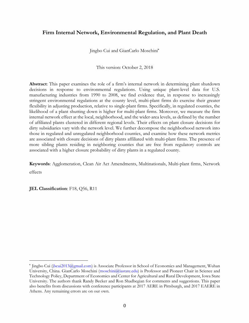
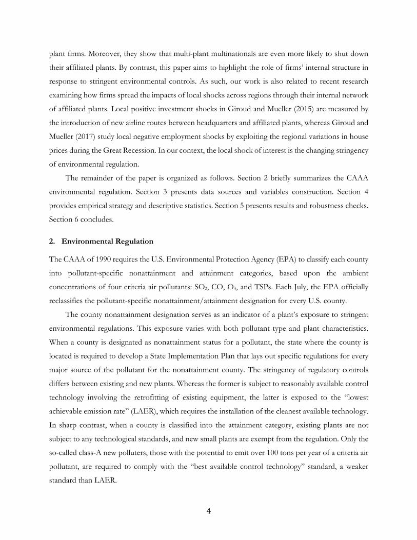
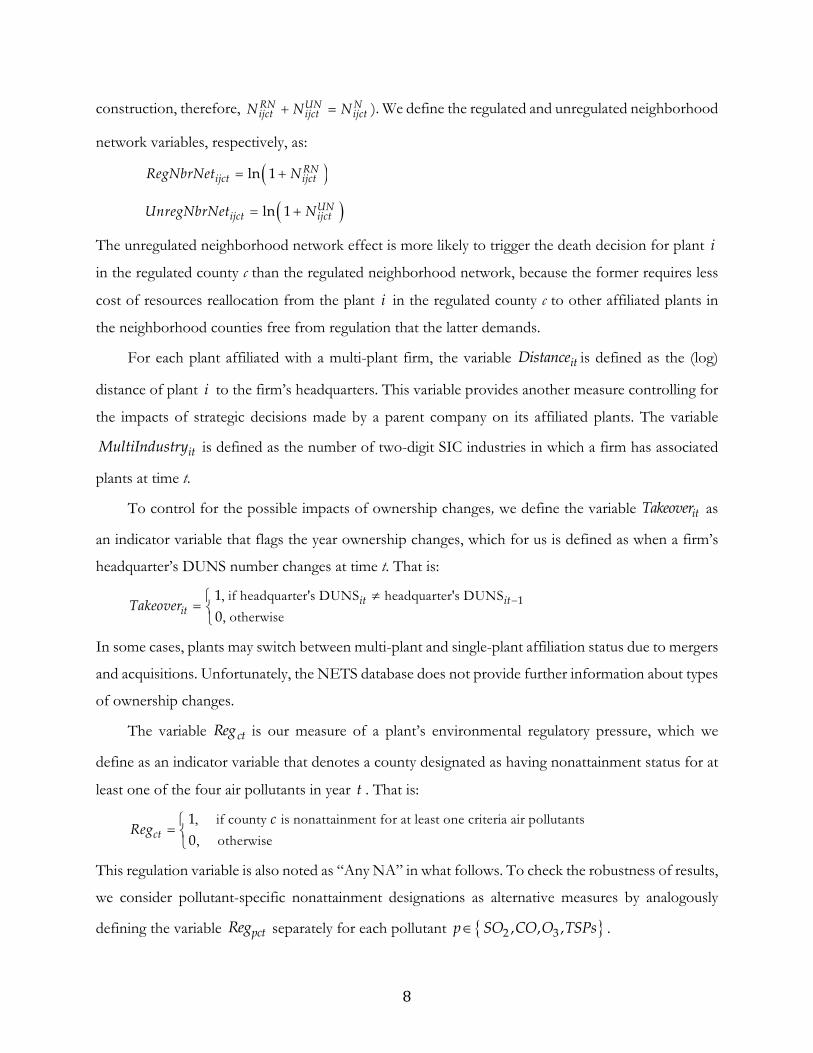
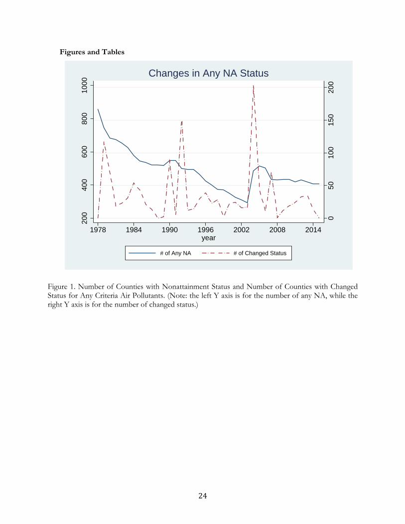
Figure 1 plots the number of counties with nonattainment status and the number of counties

with changed nonattainment status for any criteria air pollutants from 1978 to 2014.7 The data are

calculated from the EPA Green Book. The number of counties with nonattainment designations

drops steadily from over 800 in the late 1970s, when the CAAA was implemented, to around 300 in

2002. Due to the implementation of strict standards for TSPs and ground-level O3, the total number

of nonattainment counties jumps back to about 500 around 2004. Moreover, in comparison to our

sample period of 1990–2008, there exists substantial variations in county-level

nonattainment/attainment designations in both earlier and later sample periods, allowing us to identify

the effects of county-level environmental controls on plant closure decisions.

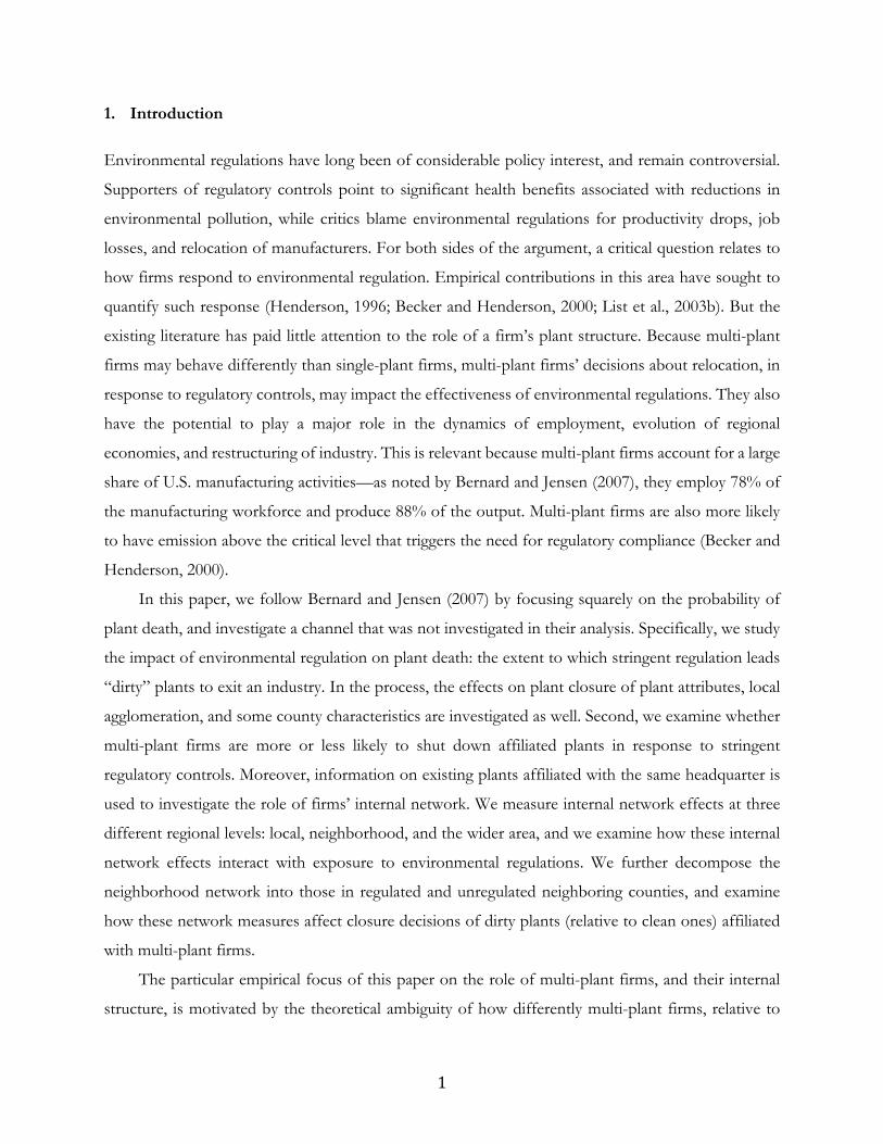
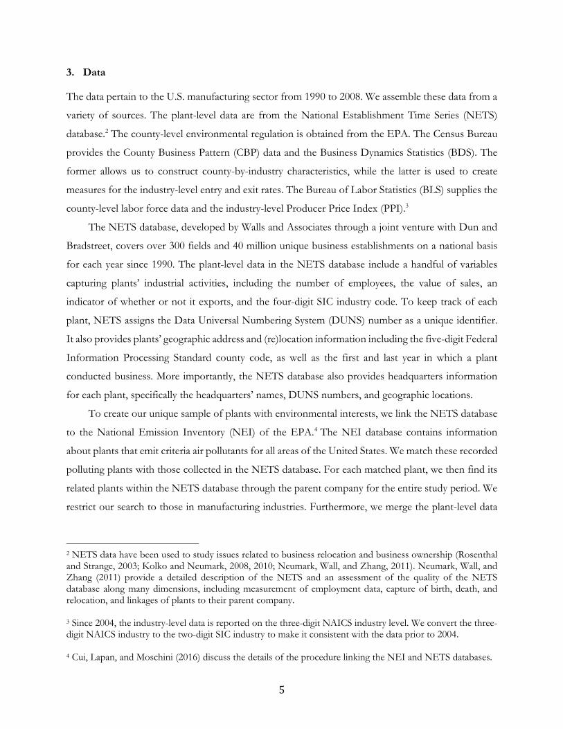
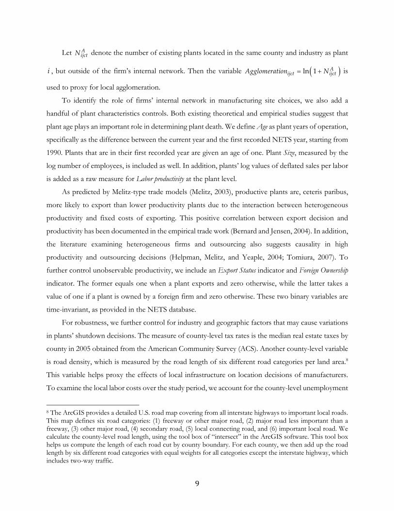
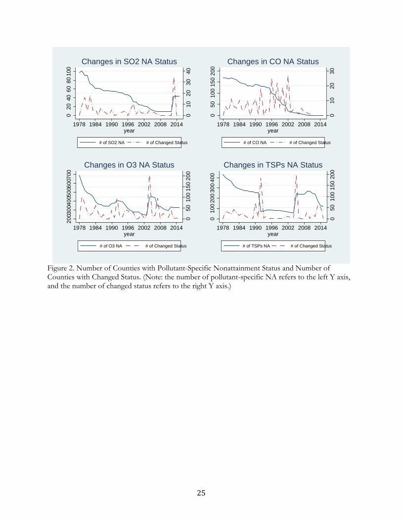
We look closely at the pollutant-specific nonattainment designations. Figure 2 decomposes the

information provided by Figure 1 for each individual pollutant. For SO2, variations in nonattainment

status are stable during the study period of 1990–2008. For CO, there are substantial variations during

the period of 1990–2002. For O3 and TSPs, significant changes in nonattainment designations mainly

occur post-CAAA (i.e., 1990–1996) and the late sample period (i.e., 2002–2008). The latter is due to

the new implementation of strict standards associated with these two pollutants.

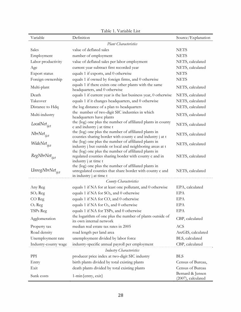
3.1 Variables

Table 1 provides a complete list and brief descriptions of variables used in this study, including the

outcome variable and other variables of interest that may be influential factors in determining plants’

site choices.

5 See http://www.epa.gov/air/oaqps/greenbk/index.html. 6 The formation of ground-level O3 is a complicated chemical process that involves Volatile Organic Compounds (VOCs) and Oxide of Nitrogen (NOx) when these two react in the presence of sunlight. We classify a county as nonattainment for O3 if it is in nonattainment for NOx and/or O3, including both one-hour and eight-hour standards. In the case of TSPs, a county is defined as TSPs-specific nonattainment when it is in nonattainment for PM10 and/or PM2.5. 7 For variations in pollutant-specific nonattainment designations at county level, see Figure 3 in the Appendix.

7

The variable Death is an indicator variable that identifies the year in which a plant shuts down. If

a plant is shut down in year 1t , the NETS database then puts t in the category of the “last year”

when business was still active. Hence, for plant i in year t this variable is defined as:

+1, if the last active year is

, otherwise

1

0it

tDeath

Multi is an indicator variable that identifies whether plant i in year t belongs to a multi-plant firm,

(i.e., if there exists at least one other plant that shares the same headquarter DUNS number) it is a

single-plant firm otherwise. Note that the multi-plant affiliation status may vary with time due to

changes in plant ownership. Hence:

, if there exists another plant with the same headquarter's DUNS number

, otherwise

1

0itMulti

To assess the effects of being associated with multi-plant firms, we create three distinct metrics

of a firm’s internal network, based upon the number of affiliated plants across regions. For a plant i

operating in industry j and located in county c , let LijctN denote the number of other plants affiliated

with the same firm that also operate in industry j and are located in county c in year t . Similarly, let

NijctN denote the number of other plants affiliated with the same firm that also operate in industry j ,

but which are located in neighboring counties (i.e., counties that share a border with county c ). Let

WijctN denote the number of other plants affiliated with the same firm that also operate in industry j

but are located outside county c and its immediate neighborhood. For single-plant firms, of course,

0L N Wijct ijct ijctN N N . Given that, we define the local network variable ijctLocalNet , the

neighborhood network variable ijctNbrNet , and the wider-area network variable ijctWideNet as:

ln 1 Lijct ijctLocalNet N

ln 1 Nijct ijctNbrNet N

ln 1 Wijct ijctWideNet N

We further distinguish the firm’s internal network in neighboring counties into regulated and

unregulated regions. Let RNijctN and UN

ijctN denote the number of neighborhood plants associated with

the same firm that are located in regulated or unregulated neighboring counties, respectively. Regulated

counties here means those designated with at least one pollutant-specific nonattainment status (by

8

construction, therefore, RN UN Nijct ijct ijctN N N ). We define the regulated and unregulated neighborhood

network variables, respectively, as:

ln 1 RNijct ijctRegNbrNet N

ln 1 UNijct ijctUnregNbrNet N

The unregulated neighborhood network effect is more likely to trigger the death decision for plant i

in the regulated county c than the regulated neighborhood network, because the former requires less

cost of resources reallocation from the plant i in the regulated county c to other affiliated plants in

the neighborhood counties free from regulation that the latter demands.

For each plant affiliated with a multi-plant firm, the variable itDistance is defined as the (log)

distance of plant i to the firm’s headquarters. This variable provides another measure controlling for

the impacts of strategic decisions made by a parent company on its affiliated plants. The variable

itMultiIndustry is defined as the number of two-digit SIC industries in which a firm has associated

plants at time t.

To control for the possible impacts of ownership changes, we define the variable itTakeover as

an indicator variable that flags the year ownership changes, which for us is defined as when a firm’s

headquarter’s DUNS number changes at time t. That is:

, if headquarter's DUNS headquarter's DUNS

, otherwise11

0it it

itTakeover

In some cases, plants may switch between multi-plant and single-plant affiliation status due to mergers

and acquisitions. Unfortunately, the NETS database does not provide further information about types

of ownership changes.

The variable ctReg is our measure of a plant’s environmental regulatory pressure, which we

define as an indicator variable that denotes a county designated as having nonattainment status for at

least one of the four air pollutants in year t . That is:

, if county is nonattainment for at least one criteria air pollutants

, otherwise

1

0ct

cReg

This regulation variable is also noted as “Any NA” in what follows. To check the robustness of results,

we consider pollutant-specific nonattainment designations as alternative measures by analogously

defining the variable pctReg separately for each pollutant 2 3, , ,p SO CO O TSPs .

9

Let AijctN denote the number of existing plants located in the same county and industry as plant

i , but outside of the firm’s internal network. Then the variable ln 1 Aijct ijctAgglomeration N is

used to proxy for local agglomeration.

To identify the role of firms’ internal network in manufacturing site choices, we also add a

handful of plant characteristics controls. Both existing theoretical and empirical studies suggest that

plant age plays an important role in determining plant death. We define Age as plant years of operation,

specifically as the difference between the current year and the first recorded NETS year, starting from

1990. Plants that are in their first recorded year are given an age of one. Plant Size, measured by the

log number of employees, is included as well. In addition, plants’ log values of deflated sales per labor

is added as a raw measure for Labor productivity at the plant level.

As predicted by Melitz-type trade models (Melitz, 2003), productive plants are, ceteris paribus,

more likely to export than lower productivity plants due to the interaction between heterogeneous

productivity and fixed costs of exporting. This positive correlation between export decision and

productivity has been documented in the empirical trade work (Bernard and Jensen, 2004). In addition,

the literature examining heterogeneous firms and outsourcing also suggests causality in high

productivity and outsourcing decisions (Helpman, Melitz, and Yeaple, 2004; Tomiura, 2007). To

further control unobservable productivity, we include an Export Status indicator and Foreign Ownership

indicator. The former equals one when a plant exports and zero otherwise, while the latter takes a

value of one if a plant is owned by a foreign firm and zero otherwise. These two binary variables are

time-invariant, as provided in the NETS database.

For robustness, we further control for industry and geographic factors that may cause variations

in plants’ shutdown decisions. The measure of county-level tax rates is the median real estate taxes by

county in 2005 obtained from the American Community Survey (ACS). Another county-level variable

is road density, which is measured by the road length of six different road categories per land area.8

This variable helps proxy the effects of local infrastructure on location decisions of manufacturers.

To examine the local labor costs over the study period, we account for the county-level unemployment

8 The ArcGIS provides a detailed U.S. road map covering from all interstate highways to important local roads. This map defines six road categories: (1) freeway or other major road, (2) major road less important than a freeway, (3) other major road, (4) secondary road, (5) local connecting road, and (6) important local road. We calculate the county-level road length, using the tool box of “intersect” in the ArcGIS software. This tool box helps us compute the length of each road cut by county boundary. For each county, we then add up the road length by six different road categories with equal weights for all categories except the interstate highway, which includes two-way traffic.

10

rate from the BLS. We also construct industry-by-county wage rate based on the ratio of annual payroll

and employment.

The magnitude of sunk entry costs is important in determining the steady-state equilibrium rate

of firm birth and death within an industry. In attempt to measure the unobserved entry costs, the

minimum of industry entry and exit rates used in Bernard and Jensen (2007) is implemented in the

regression. That is, 1 min ,jt jt jtEntryCost entryrate exitrate . The entry and exit rates computed

from the BDS are measured at the three-digit SIC industry level. Finally, to control for unobserved

industry heterogeneity, we include a full set of industry linear trends. State linear trends are also added

to absorb unobservable state characteristics varying with time.

3.2 Descriptive Statistics

Our data sample is an unbalanced panel with more than 1.2 million plant-by-year observations over

the 1990–2008 period. These observations are obtained from 153,582 unique plants affiliated with

44,069 unique headquarters.

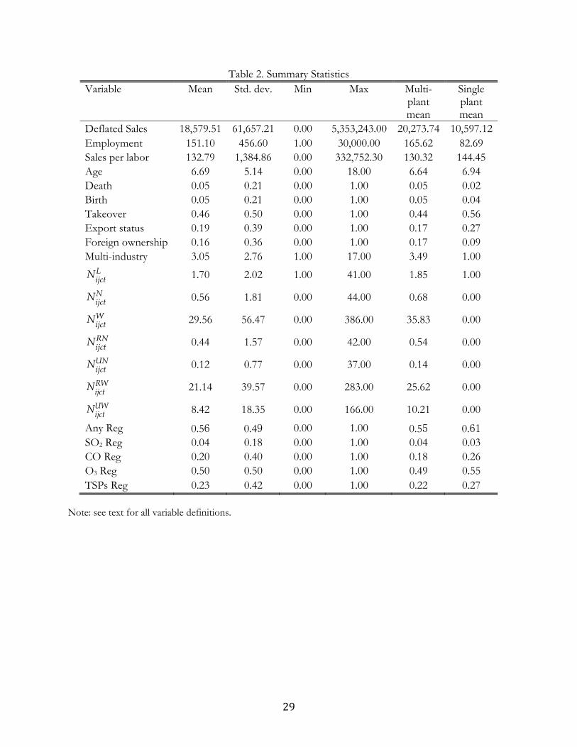
Table 2 provides summary statistics for the main variables used in the analysis. The value of sales

is deflated by the two-digit SIC industry PPI. Approximately 80% of observations are plants affiliated

with multi-plant firms, while the remaining are owned by single-plant firms. The last two columns of

Table 2 summarize the mean differences between multi-plant and single-plant status across plant

characteristics. Plants that belong to multi-plant firms are larger than those with single-plant firms in

terms of larger value of sales and more employees. However, relative to the latter, plants of multi-

plant firms have lower labor productivity measured by deflated sales per worker. When location

decisions are concerned, plants affiliated with multi-plant firms have higher death and takeover rates

than those with single-plant firms. In addition, compared with single-plant firms, multi-plant firms

have a relatively higher fraction of plants owned by foreign companies, but a lower fraction of

exporting plants. When it comes to the exposure to environmental regulations, the fraction of single-

plant firms in counties that are in nonattainment status for at least one pollutant is larger than that of

multi-plant firms residing in nonattainment counties. This result holds for all four different pollutant-

specific regulations, except SO2 nonattainment designation.

Table 3 provides mean values for plant attributes by firm structure and county nonattainment

status. For instance, plants being part of single-plant firms and located in any nonattainment counties,

on average, have 77 employees. Several interesting points arise from Table 3. First, for each type of

firm ownership, either single-plant or multi-plant, the number of plants located in nonattainment

11

counties is larger than that residing in counties free from environmental regulations. This indicates

that a substantial fraction of plants are subject to regulatory burdens. Second, plant size differs by

exposure to environmental pressures. Regardless of multi-plant status, plants residing in

nonattainment counties are younger and smaller in size (in terms of the number of employees), but

have higher labor productivity (deflated sales per worker) than those exempt from environmental

burdens. Third, regardless of multi-plant ownership, plants located in nonattainment counties have

higher death rate, but slightly lower takeover rates than those in attainment counties. When comparing

plants located in nonattainment counties, but differing in multi-plant status, multi-plant firms tend to

have larger death and takeover rates relative to similar single-plant firms. Lastly, multi-plant firms have,

on average, more subsidiaries located in nonattainment counties than in attainment counties.

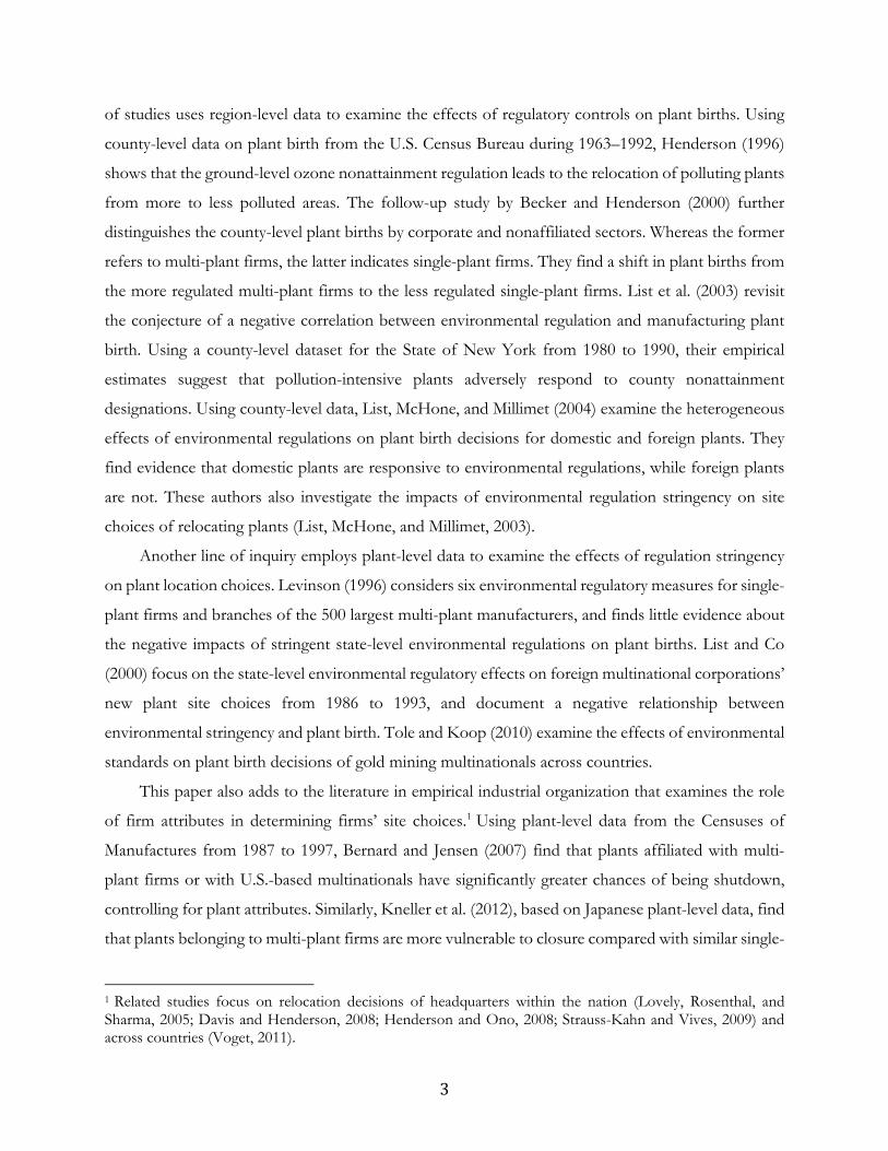
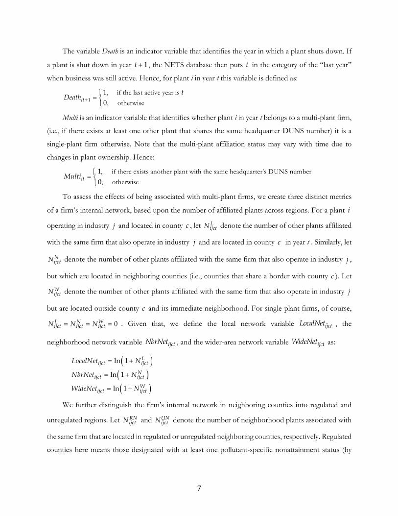
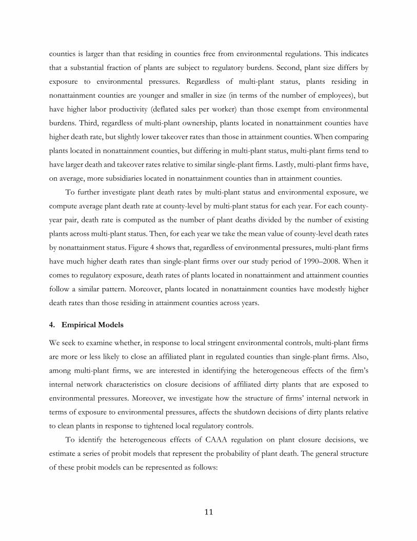
To further investigate plant death rates by multi-plant status and environmental exposure, we

compute average plant death rate at county-level by multi-plant status for each year. For each county-

year pair, death rate is computed as the number of plant deaths divided by the number of existing

plants across multi-plant status. Then, for each year we take the mean value of county-level death rates

by nonattainment status. Figure 4 shows that, regardless of environmental pressures, multi-plant firms

have much higher death rates than single-plant firms over our study period of 1990–2008. When it

comes to regulatory exposure, death rates of plants located in nonattainment and attainment counties

follow a similar pattern. Moreover, plants located in nonattainment counties have modestly higher

death rates than those residing in attainment counties across years.

4. Empirical Models

We seek to examine whether, in response to local stringent environmental controls, multi-plant firms

are more or less likely to close an affiliated plant in regulated counties than single-plant firms. Also,

among multi-plant firms, we are interested in identifying the heterogeneous effects of the firm’s

internal network characteristics on closure decisions of affiliated dirty plants that are exposed to

environmental pressures. Moreover, we investigate how the structure of firms’ internal network in

terms of exposure to environmental pressures, affects the shutdown decisions of dirty plants relative

to clean plants in response to tightened local regulatory controls.

To identify the heterogeneous effects of CAAA regulation on plant closure decisions, we

estimate a series of probit models that represent the probability of plant death. The general structure

of these probit models can be represented as follows:

12

it it it cjtProb Death X Z (1)

The outcome indicator variable itDeath was defined earlier, and ( ) denotes the cumulative

distribution function of the normal distribution. As noted earlier, i indexes a plant, j indicates the

industry of said plant, c is the county where the plant is located, and t denotes the observation year.

In equation (1), itX is a vector of regulatory and network variables that we wish to single out in our

analysis, itZ is a vector of other explanatory and control variables (including plant characteristics), and

cjt is a vector of fixed effects that control for county, industry, and time factors common to all

plants within the same county (such as county-level regulation, the measure of agglomeration

economies, and industry-by-county wage rate). The various models considered below have the

structure of equation (1) and differ in the details of the specification of the term itX .

4.1 Multi-plant vs. Single-plant Death

We explore the role of firms’ internal networks in determining plants’ responses to stringent

environmental regulations, controlling for plant, county, and industry characteristics. We test whether

a multi-plant firm, in response to tightened environmental controls, is more or less likely to shut down

its affiliated plants than a single-plant firm. Moreover, we distinguish firms’ internal network effects

with local agglomeration by utilizing the variables discussed earlier. We also consider how plant

attributes, including size, age, labor productivity, and other characteristics, are related to their

likelihood of shutting down. The county-level characteristics are also included to control for

confounding factors affecting the closure decisions of plants. The structural part of the probit model

for this analysis can be represented as

11 1 1it ct itX Reg Multi (2)

Note that because the EPA determination of nonattainment status is made in July of any given year,

our presumption is that the shutdown probability in year t is related to the status in place at the

beginning of the year (which was determined in July of year 1t ). The parameter of interest, 11 , is

the coefficient for the interaction term between the regulation variable ctReg and multi-plant

ownership dummy itMulti . This parameter captures the heterogeneous regulatory impacts on multi-

plant closure decisions relative to those with single-plant firms, controlling for local agglomeration

13

effects and county and industry characteristics.

4.2 Firm Internal Network

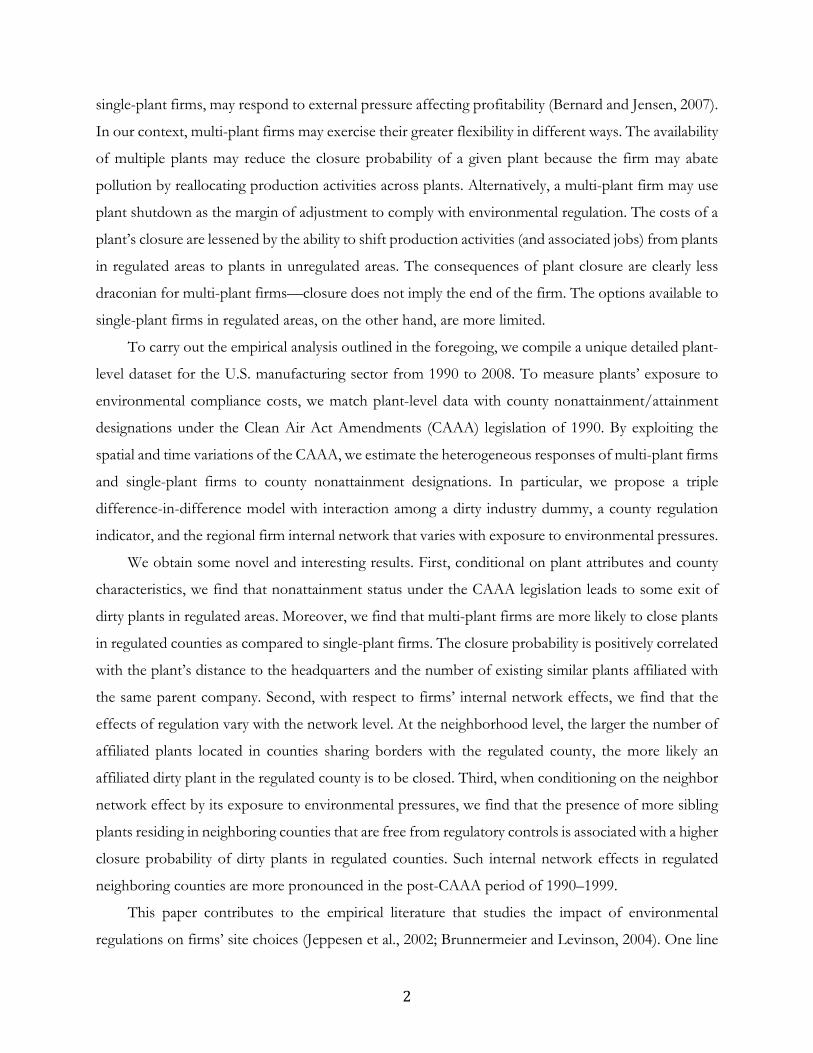
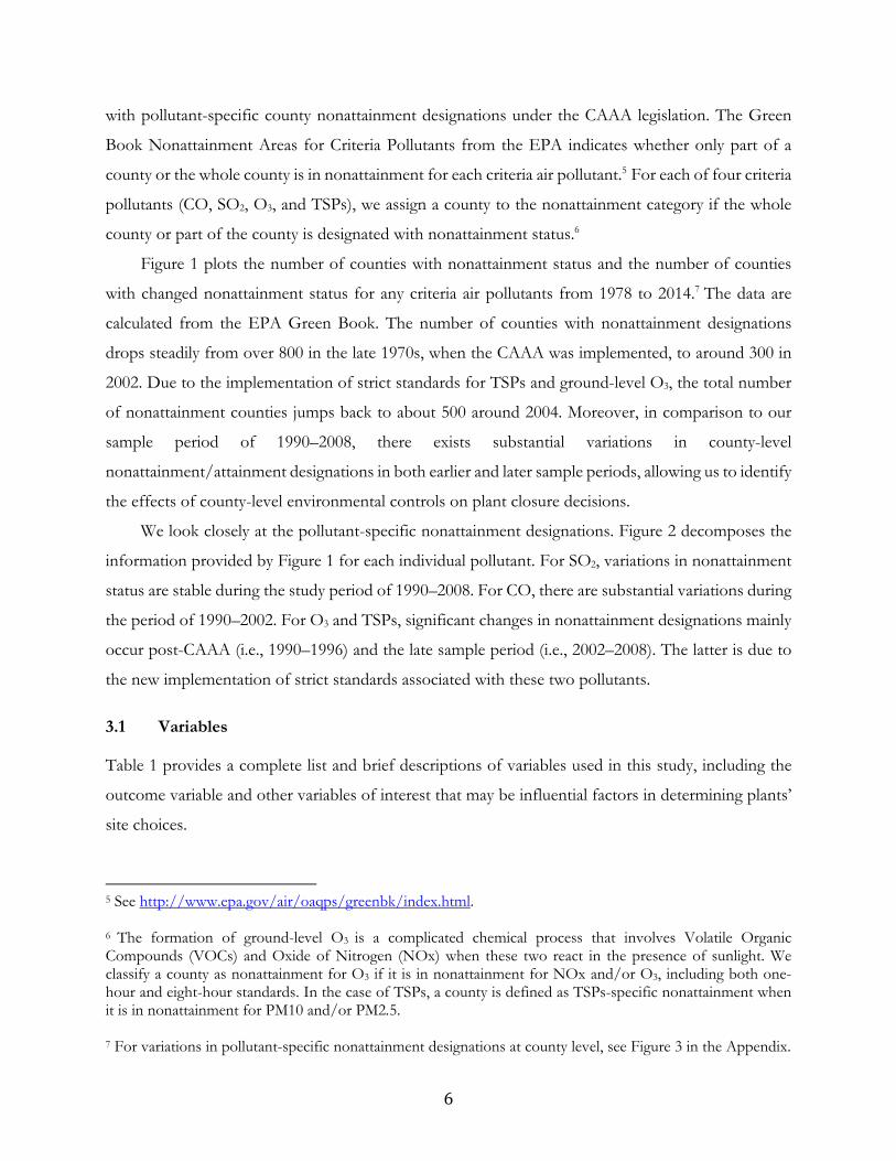
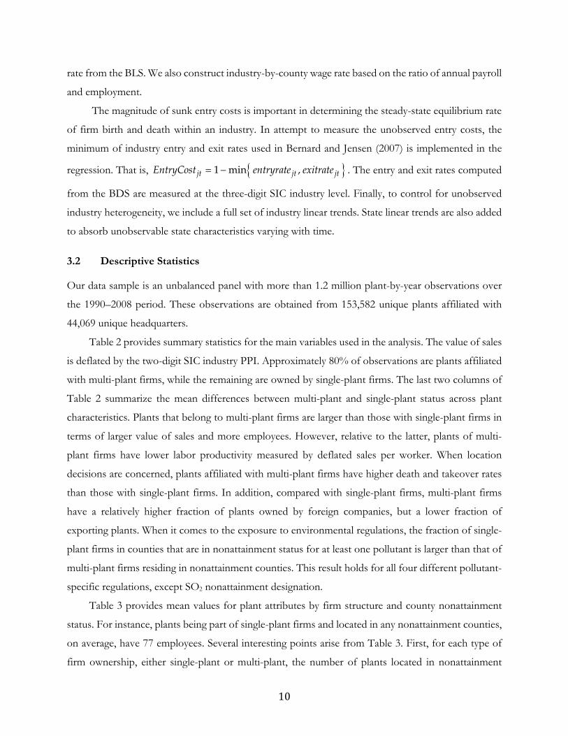
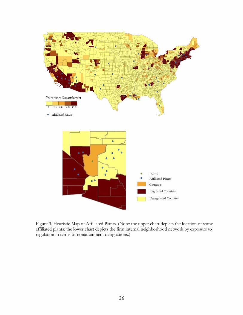
As sketched in a heuristic map in Figure 3, plants affiliated with the same parent company are located

across counties; and hence, in principle, are subject to variations in local environmental pressures.

When considering the possibility of reallocating resources from plants in regulated counties to

affiliated plants in unregulated counties, reallocation costs may vary with the distance between the

regulated plant and its affiliated plants. The distribution of sibling plants in different regional levels

may have different impacts on the probability of shutting down a plant in regulated counties and

reallocating its production resources to avoid regulatory compliance. As noted, we consider three

regional measures for firms’ internal network (local, neighborhood, and the wider area).

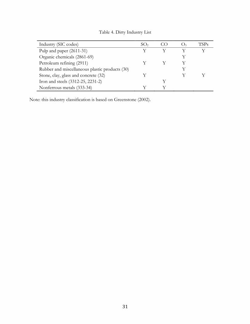
To tease out the regulatory impact on closure decisions of dirty plants, we further define dirty

plants as those in a dirty industry (i.e., industries that are known to be heavy emitters of criteria air

emissions). The classification of dirty industry is pollutant-specific and based on Greenstone (2002),

and described in Table 4. We denote jDirty as a dirty industry indicator if the industry is classified as

heavy emitters of any criteria air pollutants in the list of SO2, CO, O3, and TSPs. For each three regional

network measures, we examine the firm’s internal network effect on closure decisions for affiliated

dirty plants located in nonattainment counties by interacting the regional network variables with the

county regulatory control variable and dirty industry indicator. The county regulatory controls and

firm internal network measures are implemented in one-year lagged fashion, allowing relocation

decisions for dirty plants in the current year to respond to the stringent local environmental regulation

in the past year. Because a firm may have plants located in local, neighborhood, and wider areas, their

joint network effects may influence site choices of affiliated dirty plants in regulated counties. We add

all three network effects and their interaction terms into one specification by representing the

structural part of the probit model as follows:

+21 1 1 22 1 1

23 1 1

it j ct ijct j ct ijct

j ct ijct

X Dirty Reg LocalNet Dirty Reg NbrNet

Dirty Reg WideNet

(3)

The coefficients of interest, 21 22 23( , , ) , measure the effects of different regional networks by

comparing location responses of dirty plants with those of clean plants when both types of plants are

located in counties with strict environmental regulations. One may expect that 21 22 23( ) ,

14

indicating the heterogeneous regional firm internal network effects on closure choices of dirty plants

relative to clean plants in response to local regulatory compliance.

Next, consider a plant i that is located in a nonattainment county c, as depicted in the lower

panel of Figure 3. To avoid environmental compliance, the parent company of plant i may consider

shutting it down. The probability of shutting down plant i may be influenced by the number of

affiliated plants located in counties that share borders with county c—in particular, the number of

affiliated plants located in unregulated neighboring counties. Thus, we consider a variant specification

with the joint effects of different regional networks varying with exposure to regulations, as follows,

+

31 1 1 32 1 1

33 1 1 34 1 1

it j ct ijct j ct ijct

j ct ijct j ct ijct

X Dirty Reg RegNbrNet Dirty Reg UnregNbrNet

Dirty Reg RegWideNet Dirty Reg UnregWideNet

(4)

The coefficients 31 32 33 34( , , , ) capture how the regional firm’s internal network in regulated and

unregulated counties would affect the shutdown probability of an affiliated dirty plant relative to that

of a sibling clean plant, both of which are located in the same regulated county c. One may expect that

31 32 33 34( ) , suggesting the different effects of regional network by the variations in

environmental exposure. Moreover, one may expect 32 34( 0) , indicating that the regional

network in unregulated counties provides a potential channel of reallocating resources from dirty

plants in regulated counties to sibling plants in nearby unregulated counties. In addition, the effects of

regional firms’ internal networks on plant death declines as the distance of the network to the regulated

plant rises. The signs of 31 33( , ) , however, are ambiguous, because resource reallocation from one

dirty plant in a regulated county to its siblings in other regulated counties would not help the firm

escape from environmental compliance.

5. Results

We start by presenting results on whether multi-plant firms are more likely to close a plant than single-

plant firms in response to local environmental regulatory control. We then show how regional firms’

internal networks are involved in affecting closure decisions of dirty plants in relation to clean plants.

The effects of regional firms’ internal network interacting with exposure to environmental pressures

on plant death are presented. A series of robustness checks on model specifications, sample, and

alternative measures for firms’ internal networks are considered.

15

5.1 Multi-plant vs. Single-plant Death

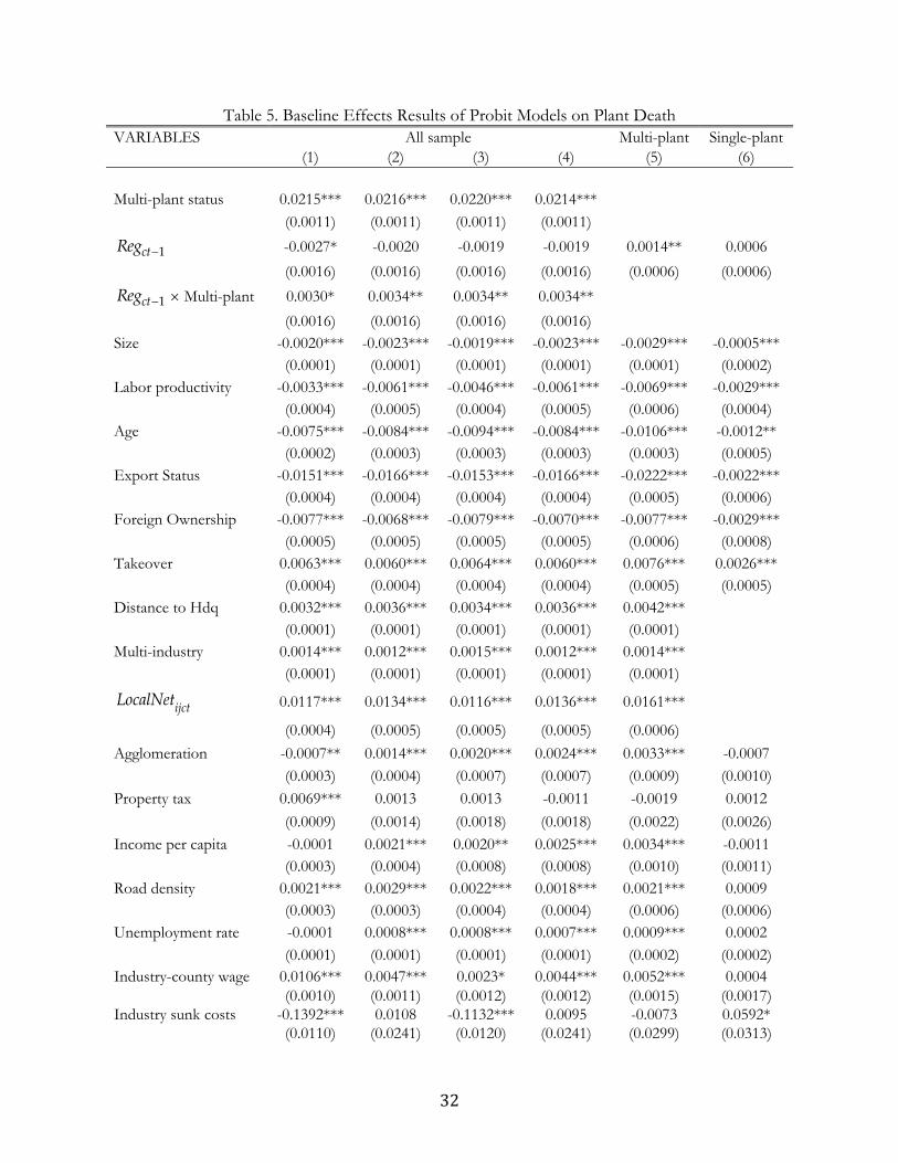
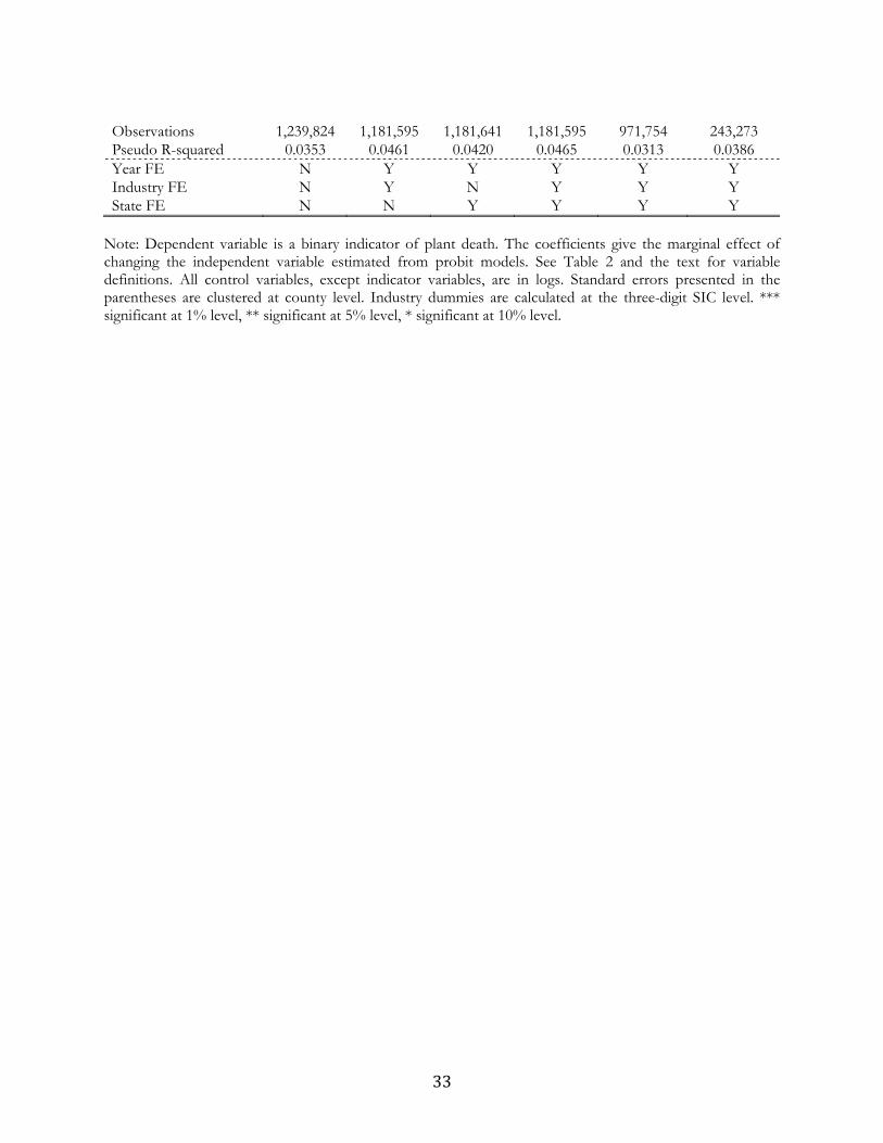
Table 5 reports estimation results for the multivariate probit models of plant death conditional on

plant and county characteristics. Whereas columns 1–4 are based on the full sample, but vary with the

choices of fixed effects as noted at the bottom of the table, the last two columns examine the sub-

samples for multi-plant and single-plant firms only, respectively. In all columns, standard errors

clustered at county level are reported in parentheses, and industry is measured by the three-digit SIC.9

The results strongly support the hypothesis that plants’ shutdown decisions are positively

associated with multi-plant status. Specifically, we find positive and statistically significant coefficients

for multi-plant affiliation status in all columns of Table 5. These estimates consistently suggest that

being affiliated with multi-plant firms significantly increases the probability of plant death at the

margin by about two percentage points. This result matches findings by Bernard and Jensen (2007),

who also conclude that multi-plant firms have greater chances of closing a plant relative to single-

plant firms, conditional on plant and county characteristics.

Moreover, we are interested in the effects of environmental regulations on plant deaths. When

splitting the data into sub-sample by multi-plant status, as shown in the last two columns of Table 5,

there are positive coefficients for the regulatory control. This positive coefficient is statistically

significant at the 1% level for the multi-plant sub-sample, while it is not statistically significant at any

conventional level for the single-plant sub-sample. The environmental controls have significant

impacts on the closure probability of plants affiliated with multi-plant firms, but not with single-plant

firms. The main focus of this paper is on the heterogeneous responses between multi-plant and single-

plant firms when both groups are subject to local regulatory controls. This heterogeneous

environmental response is captured by the coefficient for the interaction term between multi-plant

status and regulatory measure. In all columns with full sample, this coefficient is positive and

statistically significant at the 1% level. Controlling for plant attributes and county characteristics, we

find substantial differences in plant closure decisions in response to stringent regulations between

multi-plant and single-plant firms. For plants located in nonattainment counties, and hence

encountering environmental compliance, a plant that is part of a multi-plant firm has a higher

shutdown probability than a comparable single-plant firm. This finding suggests that, in compliance

with strict controls, multi-plant firms are more likely to use the plant closure margin to deal with

9 Alternative standard errors clustered at industry, county, and headquarter level are considered, but do not alter our main conclusions.

16

environmental compliance.

The effects of the firm’s internal network on plant death are examined next. We consider two

alternative measures: the (log) distant of a plant to its headquarters, and the (log) number of affiliated

plants located in the same county and in the same industry at time t. There are consistently positive

and statistically significant coefficients for these two variables across all columns in Table 5. When a

plant is located further away from its parent company, it is more likely to be shut down, as suggested

by the positive and statistically significant coefficient for the distance variable. In addition, we find

strong evidence supporting the positive effect of firms’ internal networks on plant death. The larger

the number of a firm’s affiliated plants in the same county, the higher probability an affiliated plant

would be closed. We also add a control for the number of industries that a firm’s headquarters are

involved with. This coefficient is consistently positive and statistically significant at the 1% level in all

specifications. Hence, we find that the higher the number of sub-sectors in which the headquarters

have affiliated plants, the higher the chance an affiliated plant will be closed.

When closely inspecting the relationship between plant attributes and closure likelihood, we find

negative and statistically significant coefficients for plant size, labor productivity, and age, indicating

that the probability of plant closure substantially decreases with these plant attributes. This result

implies that headquarters are more likely to shut down low-productivity and small-size plants, and that

older plants are more resilient to exiting pressure. We next consider whether exporters or multinational

firms are related to the probability of plant closure. As expected, the negative and statistically

significant coefficient shows that exporting plants have lower probability of exit (by roughly 1.6

percentage points). This result is consistent with predictions arising from the new-new trade theory

with heterogeneous firms (e.g., Melitz, 2003), showing that exporters are less likely to exit the domestic

market than their competing non-exporters. The effect of foreign ownership shows that plants owned

by foreign firms are less likely to be closed. We further examine the effects of changes in plant

ownership on plant death. As shown by the coefficient for ittakeover variable, plants experiencing

changes in ownership have higher shutdown probability. This positive coefficient is statistically

significant at the 1% level for all specifications in Table 5. The negative effect of the ownership

changes on plant closure probability is about two percentage points. One possible explanation for this

effect is that plants that have changed their ownerships are those that may behave poorly in the first

place, and hence are vulnerable to negative economic shocks.

When it comes to the effects of county characteristics on plants’ shutdown likelihood, the results

vary with the level of fixed effects included in the specification. When state or industry fixed effects

17

are present, the coefficient for local agglomeration variable is positive and statistically significant at

the 1% level, while the coefficient for local income is positive, but not significant at any conventional

levels. This piece of evidence suggests that the agglomeration effect raises plant death probability

through competition in local markets. Property tax and industry county wage rate are measures for

production costs. The estimated coefficients for these two county-level controls are positive and

statistically significant at the 1% level. This result implies that higher property tax and wage rates raise

plants’ production costs, thereby increasing the probability of death. Similarly, both the county-level

unemployment rate and road density also display positive coefficients with statistical significance at

the 1% level. The former result suggests that local unemployment rates lead to plant closure

probability, while the latter indicates that local infrastructure (perhaps surprisingly) contributes to the

exit of plants. Lastly, the industry sunk costs, measured by the entry-exit rates as in Bernard and Jensen

(2007), have negative coefficients. When the industry fixed effects are controlled to absorb the

industry-level confounding unobservable, the coefficient for the industry sunk cost does not have

statistical significance at any conventional levels, lending little support on the impacts of entry costs

on plant exit.

5.2 Regional Firm Internal Network Effects

Table 6 reports the estimated probit models for specification (3). All controls listed in column 5 of

Table 5 are included, but their coefficients are not reported in this table to save space. All columns

also include a set of year fixed effect, three-digit SIC industry linear trends and state linear trends.

Standard errors are clustered at count level.

For all three regional networks—local ( 1ijctLocalNet ), neighborhood ( 1ijctNbrNet ), and wider area

( 1ijctWideNet )—we document consistently positive impacts of regional networks interacting with the

dirty industry dummy and county regulation on plant death, as shown in columns 1–3 of Table 6.

Among all three estimated regional network effects, the neighborhood network has the largest positive

effect, which is statistically significant at the 5% level. Local and wider-area network effects, on the

other hand, are not statistically significant at conventional levels. The results are essentially unchanged

when all three regional network effects are considered simultaneously, as presented in column 4 of

Table 6. The effect that stands out is that associated with the neighborhood network. The presence

of sibling plants in neighboring counties increases the probability of a dirty plant being shutdown in a

regulated county. The local network does not exhibit the same effect: shifting resources between plants

that are subject to the same regulatory pressure does not help the firm’s environmental compliance

18

strategy.

5.3 Firm Internal Network Effects by Environmental Pressures

We further split neighborhood and wider-area networks into those in regulated areas and unregulated

areas. Table 7 provides the estimated probit models for plant death based on specification (4). In

column 1 of Table 7, we document a positive coefficient of the interaction term among the dirty

industry dummy, county regulation indicator, and neighbor network in regulated counties. This

positive effect is statistically significant at the 1% level, indicating that as more affiliated plants are

located in neighboring counties without environmental pressures, a parent company would be more

likely to close a dirty plant in the regulated county to deal with environmental compliance. Conversely,

we find little evidence of a regulated neighbor network effect. When there are some sibling plants

residing in neighboring counties also with environmental pressures, then these plants are also exposed

to environmental controls and thus are not attractive for the purpose of reallocating production

resources in order to lessen the cost of environmental compliance.

As the firm’s internal network moves to the circle outside of neighboring counties, the impact

of the regional network on plant closure is weakened. Column 2 of Table 7 shows a positive (but

insignificant) coefficient for the wider network in unregulated areas, and a negative coefficient for the

wider network in regulated areas. The latter is significant at the 1% level. Affiliated plants in

unregulated areas that are located further away from dirty plants in regulated counties have a weak or

no impact on closure decisions. Conversely, when the firm also faces environmental pressure in the

wider area, then this reduces the odds of plant closure in a given regulated county (the associated

coefficient in Table 7 is negative and statistically significant). The coefficients for the specification that

includes both neighborhood and wider area networks are reported in column 3 of Table 7. The results

are essentially the same as in columns 1 and 2.

5.4 Robustness

To check the robustness of our results, we re-conduct regression analysis based upon specification (4),

while considering different sample periods, pollutant-specific nonattainment designations, and an

alternative model specification with more controls of fixed effects.

5.4.1 Sample period

Figure 1 depicts the number of counties per year from 1978 to 2014 with changed nonattainment/

19

attainment designations. During the sample period of 1990–2008, a substantial number of counties

changed designation status during the early 1990s and the mid-2000s. The former is due to the post-

CAAA period, while the latter is because of new and strict standards for TSPs and ground-level O3

implemented around 2004. Thus, we split the whole sample period into two parts: the post-CAAA

period of 1990–1999 and the new standard period of 2000–2008. For each restricted sample period,

we re-conduct the probit model in specification (3). Table 8 reports the corresponding results. In the

post-CAAA period, as shown in columns 1–3 of Table 8, the positive effect of firms’ internal networks

on plant death in unregulated neighboring counties remains statistically significant at the 1% level.

During this period, in response to local regulatory control, headquarters are more likely to close dirty

plants and shift production to other affiliated plants in the nearby neighboring counties, which are

free from environmental regulations. Moreover, a negative and statistically significant coefficient for

firms’ internal network in wider areas without environmental pressures is again found. With more

siblings in regulated areas further away from the focal dirty plant, the likelihood of shutting down in

response to local environmental compliance declines.

In the new standard period, as shown in columns 4–6 of Table 8, coefficients of neighbor

network in unregulated counties are positive and statistically significant at the 5% level, lending

support to the conclusion that the unregulated neighbor network does impact plant death. There is

little evidence on the negative effects of the wider network in regulated areas on closure decisions of

dirty plants.

5.4.2 Pollutant-Specific Regulation

Figure 2 depicts the number of counties with changed designation status for each criteria air pollutant

under the CAAA. The pattern varies with pollutant. The changes of SO2-specific status mainly occur

in the later 1970s, and are stable during the sample period of 1990–2008. For CO, there exist

substantial changes in designations during the post-CAAA period of 1990–2002. For O3 and TSPs,

variations in designations mainly appear in the early 1990s and mid-2000s.

We consider a pollutant-specific regulation and pollutant-specific dirty industry indicator. Let

pDirty be pollutant-p-specific dirty industry dummies, following Greenstone (2002). Let 1cptReg

denote pollutant-p-specific county nonattainment status at t-1. For each pollutant p {SO2, CO, O3,

TSPs}, the following variant specification is considered:

20

+

41 1 1 42 1 1

43 1 1 44 1 1

it p cpt ijct p cpt ijct

p cpt ijct p cpt ijct

X Dirty Reg RegNbrNet Dirty Reg UnregNbrNet

Dirty Reg RegWideNet Dirty Reg UnregWideNet

(5)

where the firm’s internal network variables are defined as before.

Table 9 reports the probit model estimates on plant death during the whole sample period of

1998–2008. Columns vary with pollutant type. In response to SO2-specific regulation, the wider

network in unregulated areas raises the shutdown probability of dirty plants relative to that of clean

plants. This corresponding network effect in unregulated neighboring counties is negative but

statistically not significant. When it comes to CO- and O3-specific nonattainment designations, we

find positive coefficients for the network in unregulated neighboring counties. These positive

estimates are statistically significant at the 10% level for CO and the 1% level for O3. This finding

suggests that dirty polluters may respond to regulations by shifting resources to other affiliated plants

in the unregulated neighboring counties and then close dirty plants that are subject to CO- or O3-

specific regulatory controls. For the wide area network in regulated areas, the effect is negative and

statistically significant for O3-specific nonattainment regulation. Lastly, for TSPs the significant effect

that emerges concerns the regulated neighboring counties: the presence of sibling plants in such

counties actually reduces the shutdown probability of a dirty plant facing regulatory pressure.

5.4.3 Alternative Model Specifications

Instead of the probit model, here we estimate a linear probability model of plant death using ordinary

least square (OLS) regressions that include additional fixed effects (for the county or for the plant).

By controlling for unobserved county or plant heterogeneity, this alternative model specification

further helps tease out the causal effects for the role of the firm internal network on closure decisions

of dirty plants in response to local tough environmental controls. Table 10 presents the OLS results

of the triple interaction terms among the dirty industry dummy, one-year lagged county regulation,

and one-year lagged firm internal network.

Controlling for county or plant fixed effects, the estimated coefficients for the triple interaction

of firm internal network in unregulated neighboring counties are positive and statistically significant,

while the estimated coefficient for the triple interaction of firm internal network in regulated non-

neighboring counties are negative and statistically significant in most cases. These OLS estimates are

therefore largely consistent with those reported for the probit models.

21

6. Conclusion

In this paper we examine the role of firm structure in determining plant death in response to

increasingly stringent environmental regulation while controlling for plant attributes, headquarter

network, local agglomeration, and county characteristics. We find strong evidence of heterogeneous

responses to the stringent environmental control between multi-plant and single-plant firms. Multi-

plant firms have greater flexibility to respond to strict environmental controls. We find that plant

closure is a significant margin of adjustment for multi-plant firms. They are more likely to close

affiliated plants located in counties with stringent environmental regulations—in particular, they are

likely to shut down plants located far away from the parent company or locations with many other

similar plants in the same county. Moreover, in response to regulatory pressure, the structure of a

firm’s internal network matters. Multi-plant firms are more likely to close a plant in regulated counties

when they possess affiliated plants in counties neighboring the regulated county. This effect is mainly

driven by the firm’s internal network in unregulated neighboring counties, which is measured by the

number of affiliated plants in neighboring counties free from environmental regulations.

This paper extends our understanding on the heterogeneous regulatory impacts of environmental

regulation on firms’ production activities. Our results show that multi-plant firms do exercise their

greater flexibility in adjusting to tough environmental regulations, relative to single-plant firms.

Increasing awareness of this fact makes the design and assessment of environmental policies more

challenging. On the one hand, similar to emission leakage across borders, we may experience the

unintended consequence of emissions leakage across affiliated plants through the internal network of

multi-plant firms. On the other hand, the ability of firms to shift production activities across plants

can play a positive role by providing a cost-efficient avenue for environmental compliance, one that

can reduce emissions while minimizing the impact on production and employment. Inevitably in such

circumstances, the impacts of policy may contribute to spatial inequality, echoing concerns similar to

those arising from the impact of trade liberalization and the role of multinational firms.

22

References

Becker, R., Henderson, V., 2000. Effects of Air Quality Regulations on Polluting Industries. Journal of

Political Economy 108 (2), 379–421.

Bernard, A. B., Jensen, J. B., 2004. Why Some Firms Export. The Review of Economics and Statistics 86 (2),

561–569.

Bernard, A. B., Jensen, J. B., 2007. Firm Structure, Multinationals, and Manufacturing Plant Deaths.

The Review of Economics and Statistics 89 (2), 193–204.

Brunnermeier, S. B., Levinson, A., 2004. Examining the Evidence on Environmental Regulations and

Industry Location. The Journal of Environment & Development 13 (1), 6–41.

Cui, J., Lapan, H., Moschini, G., 2016. Productivity, Export and Environmental Performance: Air

Pollutants in the United States. American Journal of Agricultural Economics 98(2), 447-467.

Davis, J. C., Henderson, J. V., 2008. The Agglomeration of Headquarters. Regional Science and Urban

Economics 38 (5), 445–460.

Giroud, X., Mueller, H. M., 2015, Capital and Labor Reallocation within Firms, the Journal of Finance,

70(4): 1767-1804.

Giroud, X., Mueller, H. M., 2017, Firms’ Internal Networks and Local Economic Shocks, NBER

Working Paper No 23176.

Greenstone, M., 2002. The Impacts of Environmental Regulations on Industrial Activity: Evidence

from the 1970 and 1977 Clean Air Act Amendments and the Census of Manufactures. Journal of

Political Economy 110 (6), 1175–1219.

Helpman, E., Melitz, M. J., Yeaple, S. R., 2004. Export Versus FDI with Heterogeneous Firms.

American Economic Review 94 (1), 300–316.

Henderson, J. V., 1996. Effects of Air Quality Regulation. American Economic Review 86 (4), 789–813.

Henderson, J. V., Ono, Y., 2008. Where do Manufacturing Firms Locate Their Headquarters? Journal

of Urban Economics 63 (2), 431–450.

Jeppesen, T., List, J. A., Folmer, H., 2002. Environmental Regulations and New Plant Location

Decisions: Evidence from A Meta-Analysis. Journal of Regional Science 42 (1),19–49.

Kneller, R., McGowan, D., Inui, T., Matsuura, T., 2012. Closure within Multi-plant Firms: Evidence

from Japan. Review of World Economics 148 (4), 647–668.

Kolko, J., Neumark, D., 2008. Changes in the Location of Employment and Ownership: Evidence

from California. Journal of Regional Science 48 (4), 717–744.

Kolko, J., Neumark, D., 2010. Does Local Business Ownership Insulate Cities from Economic Shocks?

23

Journal of Urban Economics 67 (1), 103–115.

Levinson, A., 1996. Environmental Regulations and Manufacturers’ Location Choices: Evidence from

the Census of Manufactures. Journal of Public Economics 62 (1-2), 5–29.

List, J. A., Co, C. Y., 2000. The Effects of Environmental Regulations on Foreign Direct Investment.

Journal of Environmental Economics and Management 40 (1), 1–20.

List, J. A., McHone, W. W., Millimet, D. L., 2003. Effects of Air Quality Regulation on the Destination

Choice of Relocating Plants. Oxford Economic Papers 55 (4), 657–678.

List, J. A., McHone, W. W., Millimet, D. L., 2004. Effects of Environmental Regulation on Foreign

and Domestic Plant Births: Is There a Home Field Advantage? Journal of Urban Economics 56 (2),

303–326.

List, J. A., Millimet, D. L., Fredriksson, P. G., McHone, W. W., 2003. Effects of Environmental

Regulations on Manufacturing Plant Births: Evidence from a Propensity Score Matching

Estimator. The Review of Economics and Statistics 85 (4), 944–952.

Lovely, M. E., Rosenthal, S. S., Sharma, S., 2005. Information, Agglomeration, and the Headquarters

of U.S. Exporters. Regional Science and Urban Economics 35 (2), 167–191.

Melitz, M., 2003. The Impact of Trade on Intra-Industry Reallocations and Aggregate Industry

Productivity. Econometrica 71 (6), 1695–1725.

Neumark, D., Wall, B., Zhang, J., 2011. Do Small Businesses Create More Jobs? New Evidence for

the United States from the National Establishment Time Series. The Review of Economics and

Statistics 93 (1), 16–29.

Rosenthal, S. S., Strange, W. C., 2003. Geography, Industrial Organization, and Agglomeration. The

Review of Economics and Statistics 85 (2), 377–393.

Strauss-Kahn, V., Vives, X., 2009. Why and Where do Headquarters Move? Regional Science and Urban

Economics 39 (2), 168–186.

Tole, L., Koop, G., 2010. Do Environmental Regulations Affect the Location Decisions of

Multinational Gold Mining Firms? Journal of Economic Geography.

Tomiura, E., 2007. Foreign Outsourcing, Exporting, and FDI: A Productivity Comparison at the Firm

Level. Journal of International Economics 72 (1), 113–127.

Voget, J., 2011. Relocation of Headquarters and International Taxation. Journal of Public Economics 95

(9), 1067–1081.

24

Figures and Tables

Figure 1. Number of Counties with Nonattainment Status and Number of Counties with Changed Status for Any Criteria Air Pollutants. (Note: the left Y axis is for the number of any NA, while the right Y axis is for the number of changed status.)

050

100

150

200

200

400

600

800

1000

1978 1984 1990 1996 2002 2008 2014year

# of Any NA # of Changed Status

Changes in Any NA Status

25

Figure 2. Number of Counties with Pollutant-Specific Nonattainment Status and Number of Counties with Changed Status. (Note: the number of pollutant-specific NA refers to the left Y axis, and the number of changed status refers to the right Y axis.)

010

2030

40

020

4060

8010

0

1978 1984 1990 1996 2002 2008 2014year

# of SO2 NA # of Changed Status

Changes in SO2 NA Status

010

2030

050

100

150

200

1978 1984 1990 1996 2002 2008 2014year

# of CO NA # of Changed Status

Changes in CO NA Status

050

100

150

200

2003

0040

0500

6007

00

1978 1984 1990 1996 2002 2008 2014year

# of O3 NA # of Changed Status

Changes in O3 NA Status

050

100

150

200

010

020

030

040

0

1978 1984 1990 1996 2002 2008 2014year

# of TSPs NA # of Changed Status

Changes in TSPs NA Status

26

Figure 3. Heuristic Map of Affiliated Plants. (Note: the upper chart depicts the location of some affiliated plants; the lower chart depicts the firm internal neighborhood network by exposure to regulation in terms of nonattainment designations.)

27

Figure 4. Average County-level Plant Death Rate by Multi-Plant Status, 1990–2008. (Note: death rate is computed as the number of death plants divided by the number of existing plants by multi-plant status. Nonattainment is set for any criteria pollutants.)

28

Table 1. Variable List Variable Definition Source/Explanation Plant Characteristics

Sales value of deflated sales NETS Employment number of employment NETS Labor productivity value of deflated sales per labor employment NETS, calculated Age current year subtract first recorded year NETS, calculated Export status equals 1 if exports, and 0 otherwise NETS Foreign ownership equals 1 if owned by foreign firms, and 0 otherwise NETS

Multi-plant equals 1 if there exists one other plants with the same headquarters, and 0 otherwise

NETS, calculated

Death equals 1 if current year is the last business year, 0 otherwise NETS, calculated Takeover equals 1 if it changes headquarters, and 0 otherwise NETS, calculated Distance to Hdq the log distance of a plan to headquarters NETS, calculated

Multi-industry the number of two-digit SIC industries in which headquarters have plants

NETS, calculated

the (log) one plus the number of affiliated plants in county c and industry j at time t

NETS, calculated

the (log) one plus the number of affiliated plants in counties sharing border with county c and industry j at t

NETS, calculated

the (log) one plus the number of affiliated plants in industry j but outside or local and neighboring areas at t

NETS, calculated

the (log) one plus the number of affiliated plants in regulated counties sharing border with county c and in industry j at time t

NETS, calculated

the (log) one plus the number of affiliated plants in unregulated counties that share border with county c and in industry j at time t

NETS, calculated

County Characteristics

Any Reg equals 1 if NA for at least one pollutant, and 0 otherwise EPA, calculated SO2 Reg equals 1 if NA for SO2, and 0 otherwise EPA CO Reg equals 1 if NA for CO, and 0 otherwise EPA O3 Reg equals 1 if NA for O3, and 0 otherwise EPA TSPs Reg equals 1 if NA for TSPs, and 0 otherwise EPA

Agglomeration the logarithm of one plus the number of plants outside of its own internal network

CBP, calculated

Property tax median real estate tax rates in 2005 ACS Road density road length per land area ArcGIS, calculated Unemployment rate unemployment divided by labor force BLS, calculated Industry-county wage industry-specific annual payroll per employment CBP, calculated Industry Characteristics

PPI producer price index at two-digit SIC industry BLS Entry birth plants divided by total existing plants Census of Bureau, Exit death plants divided by total existing plants Census of Bureau

Sunk costs 1-min{entry, exit} Bernard & Jensen (2007), calculated

29

Table 2. Summary Statistics Variable Mean Std. dev. Min Max Multi-

plant mean

Single plant mean

Deflated Sales 18,579.51 61,657.21 0.00 5,353,243.00 20,273.74 10,597.12Employment 151.10 456.60 1.00 30,000.00 165.62 82.69 Sales per labor 132.79 1,384.86 0.00 332,752.30 130.32 144.45 Age 6.69 5.14 0.00 18.00 6.64 6.94 Death 0.05 0.21 0.00 1.00 0.05 0.02 Birth 0.05 0.21 0.00 1.00 0.05 0.04 Takeover 0.46 0.50 0.00 1.00 0.44 0.56 Export status 0.19 0.39 0.00 1.00 0.17 0.27 Foreign ownership 0.16 0.36 0.00 1.00 0.17 0.09 Multi-industry 3.05 2.76 1.00 17.00 3.49 1.00

1.70 2.02 1.00 41.00 1.85 1.00

0.56 1.81 0.00 44.00 0.68 0.00

29.56 56.47 0.00 386.00 35.83 0.00

0.44 1.57 0.00 42.00 0.54 0.00

0.12 0.77 0.00 37.00 0.14 0.00

21.14 39.57 0.00 283.00 25.62 0.00

8.42 18.35 0.00 166.00 10.21 0.00

Any Reg 0.56 0.49 0.00 1.00 0.55 0.61 SO2 Reg 0.04 0.18 0.00 1.00 0.04 0.03 CO Reg 0.20 0.40 0.00 1.00 0.18 0.26 O3 Reg 0.50 0.50 0.00 1.00 0.49 0.55 TSPs Reg 0.23 0.42 0.00 1.00 0.22 0.27

Note: see text for all variable definitions.

30

Table 3. Mean Value for Plant Characteristics by Firm Structure

Variable Multi-plant Single plant Any Reg = 0 Any Reg = 1 Any Reg = 0 Any Reg = 1Observations 338,069 989,772 59,705 222,123 Deflated sales 21163.99 19969.66 12240.79 10155.31 Employment 171.26 163.70 92.68 80.00 Sales per labor 124.81 132.20 141.68 145.20 Age 7.24 6.43 7.85 6.70 Death 0.051 0.055 0.018 0.017 Birth 0.050 0.050 0.042 0.038 Takeover 0.445 0.434 0.593 0.545 Export status 0.171 0.173 0.268 0.268 Foreign ownership 0.166 0.171 0.101 0.085 Multi-industry 3.475 3.492 1.000 1.000

1.742 1.884 1.000 1.000

0.560 0.720 0.000 0.000

40.104 34.371 0.000 0.000

0.208 0.649 0.000 0.000

0.352 0.071 0.000 0.000

27.742 24.896 0.000 0.000

12.361 9.476 0.000 0.000

Note: see text for all variable definitions.

31

Table 4. Dirty Industry List

Industry (SIC codes) SO2 CO O3 TSPs Pulp and paper (2611-31) Y Y Y Y Organic chemicals (2861-69) Y Petroleum refining (2911) Y Y Y Rubber and miscellaneous plastic products (30) Y Stone, clay, glass and concrete (32) Y Y Y Iron and steels (3312-25, 2231-2) Y

Nonferrous metals (333-34) Y Y

Note: this industry classification is based on Greenstone (2002).

32

Table 5. Baseline Effects Results of Probit Models on Plant Death VARIABLES All sample Multi-plant Single-plant (1) (2) (3) (4) (5) (6) Multi-plant status 0.0215*** 0.0216*** 0.0220*** 0.0214***

(0.0011) (0.0011) (0.0011) (0.0011)

1ctReg -0.0027* -0.0020 -0.0019 -0.0019 0.0014** 0.0006 (0.0016) (0.0016) (0.0016) (0.0016) (0.0006) (0.0006)

1ctReg Multi-plant 0.0030* 0.0034** 0.0034** 0.0034**

(0.0016) (0.0016) (0.0016) (0.0016)

Size -0.0020*** -0.0023*** -0.0019*** -0.0023*** -0.0029*** -0.0005*** (0.0001) (0.0001) (0.0001) (0.0001) (0.0001) (0.0002)

Labor productivity -0.0033*** -0.0061*** -0.0046*** -0.0061*** -0.0069*** -0.0029*** (0.0004) (0.0005) (0.0004) (0.0005) (0.0006) (0.0004)

Age -0.0075*** -0.0084*** -0.0094*** -0.0084*** -0.0106*** -0.0012** (0.0002) (0.0003) (0.0003) (0.0003) (0.0003) (0.0005)

Export Status -0.0151*** -0.0166*** -0.0153*** -0.0166*** -0.0222*** -0.0022*** (0.0004) (0.0004) (0.0004) (0.0004) (0.0005) (0.0006)

Foreign Ownership -0.0077*** -0.0068*** -0.0079*** -0.0070*** -0.0077*** -0.0029*** (0.0005) (0.0005) (0.0005) (0.0005) (0.0006) (0.0008)

Takeover 0.0063*** 0.0060*** 0.0064*** 0.0060*** 0.0076*** 0.0026*** (0.0004) (0.0004) (0.0004) (0.0004) (0.0005) (0.0005)

Distance to Hdq 0.0032*** 0.0036*** 0.0034*** 0.0036*** 0.0042*** (0.0001) (0.0001) (0.0001) (0.0001) (0.0001)

Multi-industry 0.0014*** 0.0012*** 0.0015*** 0.0012*** 0.0014*** (0.0001) (0.0001) (0.0001) (0.0001) (0.0001)

0.0117*** 0.0134*** 0.0116*** 0.0136*** 0.0161***

(0.0004) (0.0005) (0.0005) (0.0005) (0.0006)

Agglomeration -0.0007** 0.0014*** 0.0020*** 0.0024*** 0.0033*** -0.0007 (0.0003) (0.0004) (0.0007) (0.0007) (0.0009) (0.0010)

Property tax 0.0069*** 0.0013 0.0013 -0.0011 -0.0019 0.0012 (0.0009) (0.0014) (0.0018) (0.0018) (0.0022) (0.0026)

Income per capita -0.0001 0.0021*** 0.0020** 0.0025*** 0.0034*** -0.0011 (0.0003) (0.0004) (0.0008) (0.0008) (0.0010) (0.0011)

Road density 0.0021*** 0.0029*** 0.0022*** 0.0018*** 0.0021*** 0.0009 (0.0003) (0.0003) (0.0004) (0.0004) (0.0006) (0.0006)

Unemployment rate -0.0001 0.0008*** 0.0008*** 0.0007*** 0.0009*** 0.0002 (0.0001) (0.0001) (0.0001) (0.0001) (0.0002) (0.0002)

Industry-county wage 0.0106*** 0.0047*** 0.0023* 0.0044*** 0.0052*** 0.0004 (0.0010) (0.0011) (0.0012) (0.0012) (0.0015) (0.0017)

Industry sunk costs -0.1392*** 0.0108 -0.1132*** 0.0095 -0.0073 0.0592* (0.0110) (0.0241) (0.0120) (0.0241) (0.0299) (0.0313)

33

Observations 1,239,824 1,181,595 1,181,641 1,181,595 971,754 243,273 Pseudo R-squared 0.0353 0.0461 0.0420 0.0465 0.0313 0.0386 Year FE N Y Y Y Y Y Industry FE N Y N Y Y Y State FE N N Y Y Y Y

Note: Dependent variable is a binary indicator of plant death. The coefficients give the marginal effect of changing the independent variable estimated from probit models. See Table 2 and the text for variable definitions. All control variables, except indicator variables, are in logs. Standard errors presented in the parentheses are clustered at county level. Industry dummies are calculated at the three-digit SIC level. *** significant at 1% level, ** significant at 5% level, * significant at 10% level.

34

Table 6. Regional Firm Internal Network Effect on Plant Death

VARIABLES (1) (2) (3) (4)

jDirty × -1ctReg × 0.0130 -0.0080 (0.0314) (0.0330)

jDirty × -1ctReg × 0.0450** 0.0469* (0.0224) (0.0240)

jDirty × -1ctReg × 0.0044 0.0013 (0.0064) (0.0067)

Observations 971,754 971,754 971,754 971,754 Pseudo R-squared 0.0341 0.0341 0.0341 0.0341 Plant Control Y Y Y Y Year FE Y Y Y Y 3SIC-Industry Trend Y Y Y Y State Trend Y Y Y Y

Note: Dependent variable is a binary indicator of plant death. All controls and fixed effects in column 5 of Table 5 are included. Dirty is a dirty industry dummy for any criteria air pollutants. See text for all variable definitions. Standard errors presented in the parentheses are clustered at county level. *** significant at 1% level, ** significant at 5% level, * significant at 10% level.

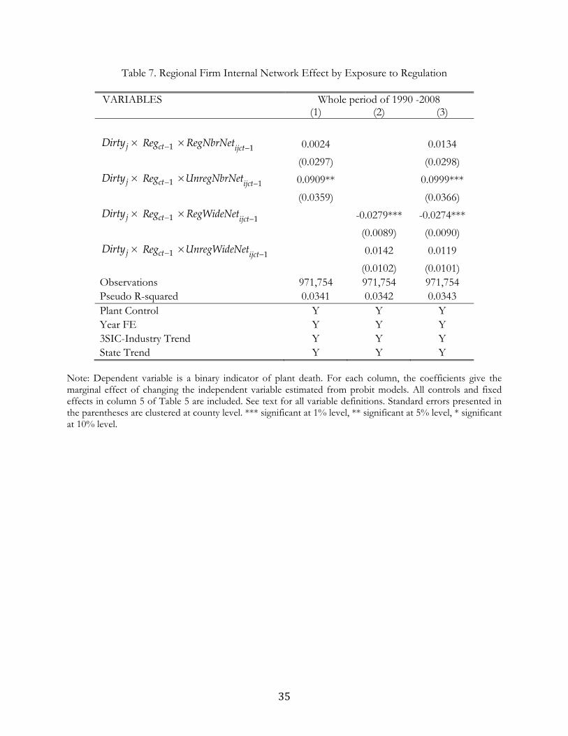
35

Table 7. Regional Firm Internal Network Effect by Exposure to Regulation

VARIABLES Whole period of 1990 -2008 (1) (2) (3)

jDirty × 1ctReg × 0.0024 0.0134 (0.0297) (0.0298)

jDirty × 1ctReg × 0.0909** 0.0999*** (0.0359) (0.0366)

jDirty × 1ctReg × -0.0279*** -0.0274*** (0.0089) (0.0090)

jDirty × 1ctReg × 0.0142 0.0119 (0.0102) (0.0101)

Observations 971,754 971,754 971,754 Pseudo R-squared 0.0341 0.0342 0.0343 Plant Control Y Y Y Year FE Y Y Y 3SIC-Industry Trend Y Y Y State Trend Y Y Y

Note: Dependent variable is a binary indicator of plant death. For each column, the coefficients give the marginal effect of changing the independent variable estimated from probit models. All controls and fixed effects in column 5 of Table 5 are included. See text for all variable definitions. Standard errors presented in the parentheses are clustered at county level. *** significant at 1% level, ** significant at 5% level, * significant at 10% level.

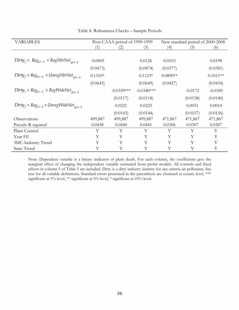
36

Table 8. Robustness Checks – Sample Periods

VARIABLES Post-CAAA period of 1990-1999 New standard period of 2000-2008 (1) (2) (3) (4) (5) (6)

jDirty × 1ctReg × -0.0005 0.0126 0.0103 0.0198 (0.0473) (0.0474) (0.0377) (0.0381)

jDirty × 1ctReg × 0.1103* 0.1123* 0.0890** 0.1011** (0.0643) (0.0649) (0.0427) (0.0434)

jDirty × 1ctReg × -0.0359*** -0.0340*** -0.0172 -0.0189 (0.0117) (0.0118) (0.0138) (0.0140)

jDirty × 1ctReg × 0.0221 0.0223 0.0051 0.0014 (0.0143) (0.0144) (0.0157) (0.0156)

Observations 499,887 499,887 499,887 471,867 471,867 471,867 Pseudo R-squared 0.0438 0.0440 0.0441 0.0306 0.0307 0.0307 Plant Control Y Y Y Y Y Y Year FE Y Y Y Y Y Y 3SIC-Industry Trend Y Y Y Y Y Y State Trend Y Y Y Y Y Y

Note: Dependent variable is a binary indicator of plant death. For each column, the coefficients give the marginal effect of changing the independent variable estimated from probit models. All controls and fixed effects in column 5 of Table 5 are included. Dirty is a dirty industry dummy for any criteria air pollutants. See text for all variable definitions. Standard errors presented in the parenthesis are clustered at county level. *** significant at 1% level, ** significant at 5% level, * significant at 10% level.

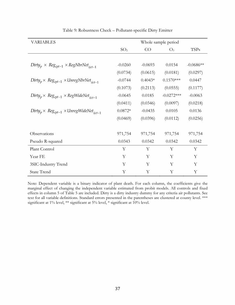
37

Table 9: Robustness Check – Pollutant-specific Dirty Emitter

VARIABLES Whole sample period SO2 CO O3 TSPs

pDirty × 1cptReg × -0.0260 -0.0693 0.0154 -0.0686** (0.0734) (0.0615) (0.0181) (0.0297)

pDirty × 1cptReg × -0.0744 0.4043* 0.1570*** 0.0447 (0.1073) (0.2113) (0.0555) (0.1177)

pDirty × 1cptReg × -0.0645 0.0185 -0.0272*** -0.0063 (0.0411) (0.0346) (0.0097) (0.0218)

pDirty × 1cptReg × 0.0872* -0.0435 0.0105 0.0136 (0.0469) (0.0396) (0.0112) (0.0256)

Observations 971,754 971,754 971,754 971,754

Pseudo R-squared 0.0343 0.0342 0.0342 0.0342

Plant Control Y Y Y Y

Year FE Y Y Y Y

3SIC-Industry Trend Y Y Y Y

State Trend Y Y Y Y

Note: Dependent variable is a binary indicator of plant death. For each column, the coefficients give the marginal effect of changing the independent variable estimated from probit models. All controls and fixed effects in column 5 of Table 5 are included. Dirty is a dirty industry dummy for any criteria air pollutants. See text for all variable definitions. Standard errors presented in the parentheses are clustered at county level. *** significant at 1% level, ** significant at 5% level, * significant at 10% level.

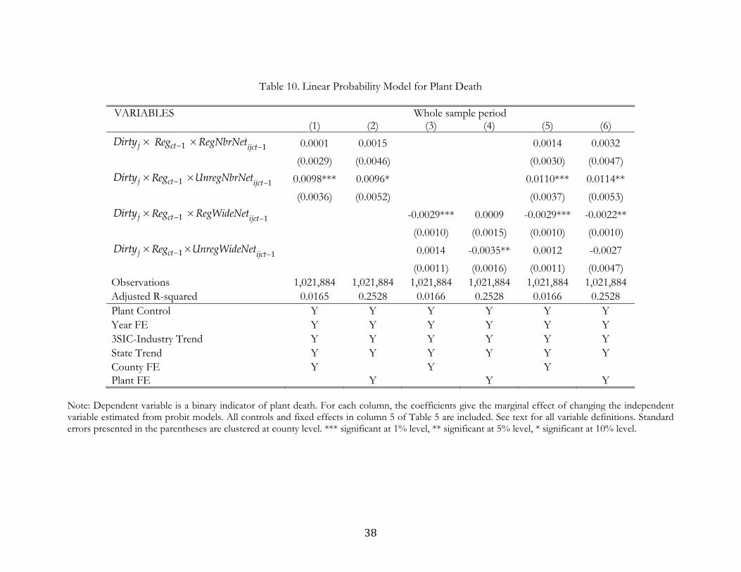
38

Table 10. Linear Probability Model for Plant Death

VARIABLES Whole sample period (1) (2) (3) (4) (5) (6)

jDirty × 1ctReg × 0.0001 0.0015 0.0014 0.0032 (0.0029) (0.0046) (0.0030) (0.0047)

jDirty × 1ctReg × 0.0098*** 0.0096* 0.0110*** 0.0114** (0.0036) (0.0052) (0.0037) (0.0053)

jDirty × 1ctReg × -0.0029*** 0.0009 -0.0029*** -0.0022** (0.0010) (0.0015) (0.0010) (0.0010)

jDirty × 1ctReg × 0.0014 -0.0035** 0.0012 -0.0027 (0.0011) (0.0016) (0.0011) (0.0047)

Observations 1,021,884 1,021,884 1,021,884 1,021,884 1,021,884 1,021,884 Adjusted R-squared 0.0165 0.2528 0.0166 0.2528 0.0166 0.2528 Plant Control Y Y Y Y Y Y Year FE Y Y Y Y Y Y 3SIC-Industry Trend Y Y Y Y Y Y State Trend Y Y Y Y Y Y County FE Y Y Y Plant FE Y Y Y

Note: Dependent variable is a binary indicator of plant death. For each column, the coefficients give the marginal effect of changing the independent variable estimated from probit models. All controls and fixed effects in column 5 of Table 5 are included. See text for all variable definitions. Standard errors presented in the parentheses are clustered at county level. *** significant at 1% level, ** significant at 5% level, * significant at 10% level.

39

Appendix

This appendix describes detailed algorithm for matching plant-level data from different sources. We

begin with polluting plants reported in the NEI database of the EPA. The NEI database contains

information about plants that emit criteria air pollutants for all areas of the United States. Since 2002,

it releases an updated version of the NEI database every three years with the latest version realeased

in 2008. Plants recorded in the NEI database emit at least one type of criteria air pollutant (i.e., CO,

SO2, TSPs, NOx, and VOCs).

Next, we match polluting plants in the NEI database with those that appear in the NETS

database, using a name and plant identifier matching algorithm. The NETS database assigns the

DUNS number to identify unique business facilities. The EPA also has information of DUNS

numbers for some polluting plants, but not all. Approximately 80% of polluting plants in the

manufacturing industry collected in the NEI database have associated DUNS numbers. However, the

EPA does not provide further information about how DUNS numbers are reported for polluting

plants and why some plants have missing DUNS numbers while others have more than one. In an

attempt to circumvent this shortcoming, we consider a pair of plants from each source as a match, if

the following series of criteria are satisfied. They must share the same DUNS number and are located

in the same county. More importantly, for each pair, we check the plant names from each source to

ensure a match. In the end, this matching procedure narrows to 18,743 unique polluting plants,

roughly half of manufacturing polluters reported in the NEI database prior to matching.

We then take these 18,743 matched polluting plants into the NETS database to search for their

related plants, which are affiliated with the same parent company (i.e., headquarters). For each plant,

the NETS reports information about its headquarters (e.g., the DUNS number, name, and location).

In addition, it tracks the headquarters’ DUNS number over the study period. Plants related to the

matched polluters that appear in the NEI database are found in the NETS database through the

headquarters’ DUNS numbers. We restrict our sample to plants in the manufacturing industry as

determined by four-digit SIC codes (between 2000 and 4000). As a consequence, we are left with

1,610,462 plant-by-year observations from 1990 to 2008, which gives us 153,582 unique plants

affiliated with 44,069 unique headquarters. Note that the number of headquarters is larger than the

number of polluting plants because, during the study period, some plants changed headquarters,

thereby bringing more headquarters and even more affiliated plants to the sample search.