Firm policies and the cross-section of CDS spreads ∗

Andrea GambaWarwick Business School

University of Warwick†

Alessio SarettoJindal School of Management

University of Texas, Dallas‡

August 7, 2013

Abstract

We solve the credit spread puzzle with a structural model of firms policies that endoge-nously replicates the empirical cross–section of credit spreads. Structural estimationof the model’s parameters reveals that the model cannot be rejected by the data, andthat endogenous investment decisions are major determinants of CDS spreads. Wealso verify that controlling for financial leverage, CDS spreads are positively related tooperating leverage, and negatively related to growth opportunities. Consistent withthe idea that growth options reduce credit risk, investments are negatively correlatedwith changes in CDS spreads.

JEL Classifications: G12, G32

∗We thank Michael Brennan, Jan Ericsson, Brent Glover, Robert Kieschnick, Ali Ozdagli, Alex Triantis,Tony Whited, and Harold Zhang for helpful comments and seminar participants at the 2012 EuropeanFinance Association, Exeter University, the First ITAM Finance Conference in Mexico City, George MasonUniversity, Georgia State University, Manchester Business School, Piraeus University Athens, University ofTexas at Austin, University of Texas at Dallas, University of Warwick, Vienna University of Economics andBusiness. We are especially thankful to Zack Liu and Ben Zhang for excellent research assistance. All errorsare our own.†Scarman Road, Coventry, UK CV4 7AL. E-mail: andrea.gamba@wbs.ac.uk‡800 West Campbell Road, Richardson, Texas 75080. E-mail: asaretto@utdallas.edu

1 Introduction

Leverage is the main determinant of credit spreads, and many structural models have been

developed to explain variation in credit spreads with variation in leverage ratios (for example,

Chen, Collin-Dufresne, and Goldstein (2009), Bhamra, Kuehn, and Strebulaev (2010), and

Chen (2010)). An important, and perhaps necessary, restriction that the econometrician

might impose on a structural model is suggested by Bhamra, Kuehn, and Strebulaev (2010),

who show that considering a sensible cross–sectional distribution of leverage is crucial even if

one is only interested in producing a model that on average generates realistic credit spreads,

leverage ratios and default frequencies, and hence solves the “credit spread puzzle” of Huang

and Huang (2003).

Realistic leverage dynamics can be reproduced only by jointly considering the financing

and investment decisions of the firm (Leary and Roberts (2005) and Hennessy and Whited

(2005)). Therefore we conjecture that investments should also be a critical part of a credit

risk model as they might help in endogenously generating a realistic cross-sectional distri-

bution of leverage.1 Moreover, considering investment decisions is also important because

it might help explain some of the variation in credit spreads. In fact, firms with the same

leverage might have different credit spreads, because they are on different investment paths

(have different growth options), and hence have different default probabilities.

In this paper, we develop a structural model of credit risk, in which heterogenous firms

react to exogenous productivity shocks by making investment and financing decisions, subject

to a number of frictions. The model therefore encompasses both dynamic capital structure

decisions as in Fischer, Heinkel, and Zechner (1989) and dynamic investments as in Zhang

(2005) and is flexible enough that it allows us to impose some cross-sectional restriction in

the estimation process. Credit risk arises in the model because of the uncertainty that the

shareholders will be willing to meet their obligations. Default is therefore an endogenous

event. Given the optimal default policy and an exogenously specified pricing kernel, we

obtain our measure of credit spread: the price (i.e., spread) of a five year credit default swap

(CDS).2

1Arnold, Wagner, and Westermann (2012) and Kuehn and Schmid (2013), include dynamic investmentsin their models in order to study the impact of asset composition (i.e., invested asset relative to growthoptions) on the riskiness of the debt. Conversely, we are interested in studying the impact that investment,through the financing gap (i.e., difference between investments and internal resources), has on the debtdecision and hence the resulting credit risk.

2While the functional form of the pricing kernel is exogenously specified, we estimate the parameters bymatching some aggregate moment conditions: the average and standard deviation of the aggregate Sharperatio, the average, standard deviation, and first difference autocorrelation of the one year real risk freerate (i.e., one year constant maturity Treasury rate). The functional form of the pricing kernel allows for

1

We estimate the parameters of the model by simulated method of moments (SMM) using

a sample of non–financial S&P 500 firms that have CDS contracts on their debt. Contin-

gent on having specified a proper set of moment conditions, SMM allows us to produce an

objective statistical test of the model. Naturally a successful structural model of credit

risk should solve the “credit spread puzzle” of Huang and Huang (2003), while allowing the

econometrician to impose a restriction on the cross-section as in Bhamra, Kuehn, and Stre-

bulaev (2010). Therefore, we specify two sets of moment conditions: first, we demand the

model to match the unconditional average book leverage, the unconditional one-year default

frequency, and the unconditional average senior secured five year CDS spread. Second, we

require the model to match the cross-sectional distribution of credit spreads, represented by

the average CDS spreads of ten decile portfolios obtained by sorting firms based on their

book leverage.

The estimation exercise is quite successful: first, the model cannot be rejected by the

data. Second, the estimation is generally able to reconcile the credit spread “puzzle” of

Huang and Huang (2003): the model generates an average credit spread very close to the

one that is empirically observed, while at the same time requiring average leverage and

default frequency that are also close to the empirical counterparts. Third, the average

cross–sectional pricing error is very small (at 6.4 basis points): the model can accurately

reproduce the average CDS of all leverage portfolio. Fourth, we find that having a dynamic

investment policy is a central requirement for the ability of the model to match the data. A

version of the model whit fixed asset is, in fact, rejected by the data and unable to overcome

another limitation of structural models that was originally highlighted by Huang and Huang

(2003) in that it cannot generate reasonable credit spreads for firms that have very low

leverage (high credit standing). Finally, we find that frictions that have been found to

be very important determinant of leverage dynamics, such as transaction costs related to

external financing, appear to play a minor role in influencing the credit risk of a firm.

The results described above, which are produced using variation in leverage as a source of

conditional information, outlines the importance of considering variation in asset dynamics

in characterizing the cross-sectional distribution of credit spreads. The past, current, and

future investment choices are expected to impact credit risk because of two key aspects

of the model. First, the exogenous productivity shocks that affect the firms exhibit mean-

reversion. This generates persistence and mean-reversion in the firm’s profitability. Second,

countercyclical risk premia. Countercyclical risk premia have been found to be an essential feature of asuccessful pricing kernel in several studies of credit spreads and equity returns. For example, Zhang (2005),Chen, Collin-Dufresne, and Goldstein (2009), Bhamra, Kuehn, and Strebulaev (2010), Gomes and Schmid(2010), and Chen (2010).

2

adjustments to the capital stock incur asymmetric costs, as for example in Hennessy and

Whited (2005) and Zhang (2005). While in good states of the world, the option to grow

(i.e., making investments in the future) is valuable to bondholders as it is indicative of future

profitability and solvency, in bad states of the world, having not realized the option to grow

is valuable to bondholders as it spares the possibly large downsizing costs.

As Hennessy and Whited (2005) suggests, investigating the impact of conditional in-

formation that is not used in the estimation procedure gives “a measure of the success of

the out–of–sample performance of the model.” Therefore, we investigate how variation in

credit spreads is associated to observable characteristics that are a direct consequence, in

the model, of dynamic choices that firms make about their asset structure. We concen-

trate on the firm’s actual production capacity and cost structure (operating leverage), on

the prospects for the future production capacity (growth options) and on the realization of

these prospects (investments). We investigate these relationships by juxtaposing a sample

of empirically observed firms to a simulated economy.

Based on our model, we expect and find, a positive relation between credit spreads and the

current production capacity and costs structure, as measured by the firm’s operating leverage,

after controlling for financial leverage. High operating leverage, due to the predominance of

fixed costs and other overheads on variable costs, makes firms particularly inflexible in bad

states of the economy. Therefore, firms with high operating leverage have high downside

cash flow risk, and consequently higher probability of not meeting their debt obligations.

We also anticipate, and find, a negative relationship between credit spreads and growth

options, after controlling for leverage. Large growth options, because of the persistence in

the profitability process, are indicative of future expected profitability and of the possibility

to expand the firm, which in turn are positively related to the future ability of the firm to

repay current debt. As the relationship between leverage and credit spreads is non–linear,

the relation between growth options and credit spreads is also stronger (more negative)

for firms with high leverage. Moreover, as the growth options are realized through an

expansion of the capital stock, the position of debt holders is improved as a consequence of

the increase in the collateral value of the debt, thus delivering a negative relationship between

changes in credit spreads and investments. Similarly, a contraction of the firm decreases

the credit standing of the firm because of the decrease in the collateral and because of the

disinvestment cost that the firm has to absorb. Furthermore, because the asset adjustment

costs are asymmetric, the amount by which disinvestments increase credit spreads is much

larger than the amount by which investments decrease credit spreads.

3

Our paper complements recent contributions in the credit risk literature in several ways.

Huang and Huang (2003) show that traditional structural models of credit risk, similar to

Merton (1974) and Leland (1994), are not able to solve the “credit spread puzzle.” Such

models, when endowed with leverage ratios and default probabilities close to those empirically

observed, cannot generate realistic credit spreads. Chen, Collin-Dufresne, and Goldstein

(2009) propose an extension of the traditional Merton (1974) framework by introducing habit

formation into a pricing kernel that provides counter-cyclical risk premia. This innovation

allows the standard Merton model, in which the capital structure is static and there is

no investment, to produce an average credit spread on corporate debt similar to the one

empirically observed in the BBB credit class, while matching the average leverage and the

average default probability of BBB firms. Bhamra, Kuehn, and Strebulaev (2010) and

Chen (2010) extend the above framework of state dependent risk premia to the case in

which firms can dynamically adjust their capital structure through issuance of new debt,

while the asset follows an exogenous stochastic process. Chen (2010) show the importance

of considering pro-cyclical recovery rates. Bhamra, Kuehn, and Strebulaev (2010) highlight

the benefit of imposing an initial cross-sectional distribution of leverage (equal to the one

that is empirically observed), and by taking advantage of the non-linear relationship between

leverage and credit spreads. Relative to these papers, we concentrate our attention on the

cash flow generating process, while retaining the variation in risk premia; we allow firms to

follow an endogenous dynamic investment strategy; and we do not require any particular

starting point of the cross-sectional distribution of leverage, but instead endogenously obtain

a realistic unconditional distribution through the investment channel.

Two very recent papers, by Arnold, Wagner, and Westermann (2012) and Kuehn and

Schmid (2013), also aim to solve the credit spread puzzle by allowing the firm to dynamically

adjust the asset in place. In particular, Arnold, Wagner, and Westermann (2012) model

a firm that can exercise an option to expand, while hypothesizing that capital structure

is static, although optimally decided at the beginning of the life of the company. Kuehn

and Schmid (2013) model a firm that can simultaneously adjust its capital structure and

the production capacity in response to fluctuations to both idiosyncratic and systematic

shocks. One main difference between Arnold, Wagner, and Westermann (2012) and our

paper is that in their paper the actual cross-section of firms is used as a starting point

for the simulated sample, while in our the distributions of leverage and asset value are

endogenously generated. Our model shares many features with the one proposed by Kuehn

and Schmid (2013). Differently from them, we make use of a very simple pricing kernel that

allows us to estimate all the parameters of the model. Differently from Arnold, Wagner,

and Westermann (2012) and Kuehn and Schmid (2013), we estimate the parameters of

4

our model by simulated method of moments and use data on an economically important

panel of firms. Most importantly, our approach highlights the importance of considering

cross-sectional restrictions, as for example in Bhamra, Kuehn, and Strebulaev (2010), when

attempting to solve the credit spread puzzle. A significant benefit of which is to provide

new insights on cross-sectional pricing relationships, as opposed to solely focusing on solving

the credit spread puzzle.

The paper has the following structure. In Section 2, we introduce the model. In

Section 3, we discuss the data. Section 4 describes the model estimation procedure. In

Section 5, we study the relationship between credit spreads and firm policies. Our concluding

remarks are presented in Section 6.

2 The Model

We propose a partial equilibrium dynamic model of corporate decisions that is characterized

by firm heterogeneity and endogenous default. The model is therefore similar, in spirit, to

that of Hennessy and Whited (2007) in the description of the firm’s decisions, and to those

of Berk, Green, and Naik (1999), Zhang (2005) and Gomes and Schmid (2010) in the choice

of a reasonably simple structure for pricing corporate securities.

In what follows, we first characterize an economy composed by heterogenous firms in

which the preferences of risk averse investors are summarized by an exogenously specified

stochastic discount factor. Then, we describe the firm’s decisions. The model is solved using

standard dynamic programming techniques and, when possible, we refer to the terminology,

notation, and results by Stokey and Lucas (1989).

2.1 The Economy

Information is revealed and decisions are made at a set of discrete dates 0, 1, . . . , t, . . ..The time horizon is infinite. The economy is composed by a utility maximizing represen-

tative agent and a fixed number of heterogenous firms that produce the same good. Firms

make dynamic investment and financing decisions, and can default on their debt obligations.

Defaulted firms are restructured and then continue operations, so as to guarantee a constant

number of firms in the economy. The agent consumes the dividends paid by the firms and

saves by investing in the financial market. We do not derive the economy equilibrium, but

instead close the economy by choosing an exogenously specified stochastic discount factor.

5

There are two sources of risk that capture variation in the firm’s productivity. The first,

zj, is of idiosyncratic nature and captures variations in productivity caused by firms’ specific

events. The sub-script j denotes that the risk is unique to firm j. Idiosyncratic shocks are

independent across firms, and have a common transition function Qz(zj, z′j). zj denotes the

current (or time–t) value of the variable, and z′j denotes the next period (or time–(t + 1))

value.

The second source of risk, x, is of aggregate nature and captures variations in productivity

caused by macroeconomics events. The aggregate risk is independent of the idiosyncratic

shocks and has transition function Qx(x, x′).

Qz and Qx are stationary and monotone Markov transition functions that satisfy the

Feller property. z and x have compact support. For convenience of exposition, we define

the state variable s = (x, z), whose transition function, Q(s, s′), is defined as the product of

Qx and Qz. Moreover, as there is no risk of confusion, we drop the index j in the rest of

the section.

2.2 Firm Policies

We assume that firm’s decisions are made to maximize shareholders’ value. An intuitive

description of the chronology of the firm’s decision problem is presented in Figure 1. At t

the two shocks s = (x, z) are realized, and the firm cash flow is determined based on current

capital stock, k, and debt, b. Immediately after that, the firm simultaneously chooses the

new set of capital, k′, and debt, b′ for the period ]t, t + 1]. This decision determines d,

the residual cash flow to shareholders, which can be positive (a dividend) or negative (an

injection of new equity).

At t, the cash flow from operations (EBITDA) depends on the idiosyncratic and aggregate

shocks, and on the current level of asset in place, k > 0:

π = π(x, z, k) = ex+zkα − fk,

where α < 1 models decreasing returns to scale and f ≥ 0 is a fixed cost parameter that

summarizes all operating expenses excluding interest on debt.3

The capital stock of the firm might change over time. The asset depreciates both

3A fixed cost proportional to capital stock is similar to what is assumed by Carlson, Fisher, and Gi-ammarino (2004), Cooper (2006), and Kuehn and Schmid (2013).

6

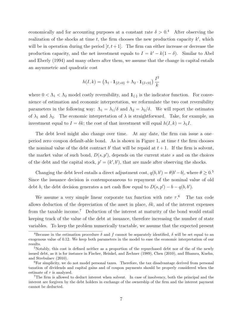
economically and for accounting purposes at a constant rate δ > 0.4 After observing the

realization of the shocks at time t, the firm chooses the new production capacity k′, which

will be in operation during the period ]t, t+ 1]. The firm can either increase or decrease the

production capacity, and the net investment equals to I = k′ − k(1 − δ). Similar to Abel

and Eberly (1994) and many others after them, we assume that the change in capital entails

an asymmetric and quadratic cost

h(I, k) =(Λ1 · 1I>0 + Λ2 · 1I<0

) I2k

where 0 < Λ1 < Λ2 model costly reversibility, and 1· is the indicator function. For conve-

nience of estimation and economic interpretation, we reformulate the two cost reversibility

parameters in the following way: Λ1 = λ1/δ and Λ2 = λ2/δ. We will report the estimates

of λ1 and λ2. The economic interpretation of λ is straightforward. Take, for example, an

investment equal to I = δk; the cost of that investment will equal h(I, k) = λ1I.

The debt level might also change over time. At any date, the firm can issue a one–

period zero–coupon default-able bond. As is shown in Figure 1, at time t the firm chooses

the nominal value of the debt contract b′ that will be repaid at t+ 1. If the firm is solvent,

the market value of such bond, D(s, p′), depends on the current state s and on the choices

of the debt and the capital stock, p′ = (k′, b′), that are made after observing the shocks.

Changing the debt level entails a direct adjustment cost, q(b, b′) = θ|b′−b|, where θ ≥ 0.5

Since the issuance decision is contemporaneous to repayment of the nominal value of old

debt b, the debt decision generates a net cash flow equal to D(s, p′)− b− q(b, b′).

We assume a very simple linear corporate tax function with rate τ .6 The tax code

allows deduction of the depreciation of the asset in place, δk, and of the interest expenses

from the taxable income.7 Deduction of the interest at maturity of the bond would entail

keeping track of the value of the debt at issuance, therefore increasing the number of state

variables. To keep the problem numerically tractable, we assume that the expected present

4Because in the estimation procedure δ and f cannot be separately identified, δ will be set equal to anexogenous value of 0.12. We keep both parameters in the model to ease the economic interpretation of ourresults.

5Notably, this cost is defined neither as a proportion of the repurchased debt nor of the of the newlyissued debt, as it is for instance in Fischer, Heinkel, and Zechner (1989), Chen (2010), and Bhamra, Kuehn,and Strebulaev (2010).

6For simplicity, we do not model personal taxes. Therefore, the tax disadvantage derived from personaltaxation of dividends and capital gains and of coupon payments should be properly considered when theestimate of τ is analyzed.

7The firm is allowed to deduct interest when solvent. In case of insolvency, both the principal and theinterest are forgiven by the debt holders in exchange of the ownership of the firm and the interest paymentcannot be deducted.

7

value of the interest payment, PI(s, p′) = b′ −D(s, p′), can be expensed when the new debt

is issued at time t. In case of linear corporate tax, and assuming knowledge of the correct

conditional default probability, this is equivalent to the standard case of deduction at t+ 1.

The after–tax cash flow from operations plus the net proceeds from the debt decision is

v = v(s, p, p′) = (1− τ)π + τδk + τPI(s, p′) +D(s, p′)− q(b, b′)− b. (1)

We incorporate insolvency on a cash flow basis as an additional element to standard

trade-off costs that are already present in our model. The firm is insolvent on a cash flow

basis, v < 0, if the after–tax cash flow from operations plus the proceeds from the new debt

issuance is lower than the value of the debt that is due. In this case, if the default option is

not exercised by shareholders, the company must raise enough new equity capital to cover

the cash shortfall and pays a proportional transaction cost ξ ≥ 0. In other words, to raise

capital for v < 0, the firm pays a cost vξ. The rationale for modeling cash flow illiquidity

stems from the fact there are some financial penalties associated with high leverage (for

example, the loss of intangible assets and the disruption of operations) which are paid by

shareholders and are hard to measure. These costs are included in our framework in a

reduced form by assuming that, in case of financial distress, the firm receives only a portion

of the capital that is injected by the shareholders.

The equity payout is therefore equal to

w = w(s, p, p′) =[v(1 + ξ · 1v<0)

]− [I + h(I, k)]

where the terms in the first square bracket represent the after–tax cash flow from operations,

inclusive of the distress cost if the firm is insolvent on a cash flow basis, and the terms in the

second square bracket represent the cash flow from investment or disinvestment. Finally,

the distribution to shareholders at t is equal to

d = d(s, p, p′) = w(1 + ϕ · 1w<0). (2)

If the distribution is positive, the firm pays a dividend to the current shareholders. If

the distribution is negative, the firm issues new shares, and d reflects the amount of equity

capital received by the company. In this case, the company incurs a proportional equity

issuance cost ϕ ≥ 0.

8

2.3 The Value of Corporate Securities

Following Berk, Green, and Naik (1999) and more recently Zhang (2005) and Gomes and

Schmid (2010), we exogenously define a pricing kernel that depends on the aggregate source

of risk, x. The associated one–period stochastic discount factor M(s, s′) defines the risk-

adjustment corresponding to a transition from the current state x to state x′. We assume

that M is a continuous function of both arguments.

The firm can issue two types of securities, debt and equity, which are both priced under

rational expectations in a perfectly efficient market.

In dynamic programming terms, the cum–dividend price of equity, S(s, p), is equal to

the sum of current distribution, d, and the present value of the expected future optimal

distributions, which is equal to the next period price S(s′, p′). Since this sum can be

negative, a limited liability provision is also included, in which case the firm is worth zero

to the shareholders:

S(s, p) = max

0,max

p′d(s, p, p′) + Es [M(s, s′)S(s′, p′)]

. (3)

The value function, S, is the solution of the functional equation (3). The ensuing

stationary optimal policy is defined as follows. The event of default is captured by the

indicator function ω = ω(s, p). If currently there is not default, the optimal investment and

financing decision is F (s, p) = (k∗, b∗).

We now turn to the evaluation of the debt contract. The payoff to debt holders at the

end of next period depends on the currently decided asset and debt, p′ = (k′, b′), the new

realization of the shocks s′, and on whether the firm is solvent or in default,

u(s′, p′) = b′(1− ω(s′, p′)) + [π′ + τδk′ + k′(1− δ)] (1− η)ω(s′, p′). (4)

The first term on the right–hand side is the payoff to debt holders in case the firm is solvent.

The second term represents the payoff in case of default. In this instance, similarly to Hen-

nessy and Whited (2007), the bondholders receive the sum of the cash flow from operations,

π′ = π(s′, k′), the depreciated book value of the asset, and the tax shield from depreciation,

all net of a proportional bankruptcy cost, η. Hence, the current value of the debt, at the

time it is issued, equals

D(s, p′) = Es [M(s, s′)u(s′, p′)] . (5)

9

One final item that needs to be evaluated is the expected present value of the interest

payment, PI(s, p′), which enters the determination of the taxable income in Equation (1),

PI(s, p′) = [b′ −D(s, p′)]Es [M(s, s′)(1− ω(s′, p′))] (6)

Because the interest is deductible only if the firm is not in default, the expectation term is

the conditional price of a default contingent claim.

In Appendix A, we prove the existence of the solution of the program given by the

Bellman operator in equation (3), subject to the constraints in equations (5) and (6). The

model is solved numerically by simultaneously finding the optimal value of S, D and PI.

We describe the numerical approach in Appendix B.

2.4 Credit Default Swap Spread

A credit default swap (CDS) is a contract whereby the protection seller pays, at default of a

given name, an amount equivalent to the protection buyer’s loss given default. The payment

is a proportion of the par value of the obligation. In exchange, the buyer periodically pays

to the seller a sequence of premium payments in arrears until the natural maturity of the

contract or until the reference name defaults, whichever happens sooner. At the inception of

the contract, the premium (i.e., CDS spread) is determined so that the sum of the expected

payments from the protection buyer equals the expected payment from the protection seller.

Let us consider a credit default swap agreement with maturity equal to T periods. The

reference entity is the issuer of an obligation with par value of one unit that can default

only at the end of each period. For notational simplicity, in this section, we revert to time

subscripts: so that st = s and st+1 = s′. Let H(st, st+1) be the price of a contingent claim

that pays $1 if state st+1 occurs and the current state is st:

H(st, st+1) = Q(st, st+1)M(st, st+1)

Let us now define the price of another contingent claim that pays $1 only if the reference

entity defaults for the first time on the obligation n periods from now as

Pn(s, p, p′) = Pn(st, pt, pt+1)

= Est[H(st+n−1, st+n)ω(st+n, pt+1)

∏n−1j=1 H(st+j−1, st+j) (1− ω(st+j, pt+1))

]and the price of a contingent claim that pays $1 if the reference entity does not default

10

within the first n periods as

Sn(s, p, p′) = Sn(st, pt, pt+1) = Est

[n∏j=1

H(st+j−1, st+j) (1− ω(st+j, pt+1))

]

Note that, in the above definitions, the firm’s policy, p′ = pt+1, does not change from one

period to the other; the only part evolving through time is the exogenous state. This is

an important point to note because, when estimating the parameters, we ask the model to

price a CDS contracts with a five year maturity. To do so we need to compute the five year

cumulative default probability, and we are therefore assuming that the firm’s choice of debt

and capital would not change with the aggregate and idiosyncratic shocks. To assure that

this assumption is not overly stringent, we will avoid the problem entirely, and repeat the

estimation procedure using a one year CDS as the reference security.

Finally, the CDS spread is

cds(s, p, p′) = (1−R)

∑Tn=1Pn(s, p, p′)∑T

n=1 (Pn(s, p, p′) + Sn(s, p, p′))(7)

where R is the recovery on the face value of a unit bond.

3 Data

The data used in the model estimation and in the rest of the analysis is assembled from

different datasets. The data used to estimate the parameters of the stochastic discount factor

model is obtained from the Federal Reserve Economic Data (FRED) Saint Louis and from

Professor Kenneth French’s website. In particular we obtain the one year constant maturity

Treasury rate and the consumer price index for all urban consumers from FRED. We obtain

the returns on a value-weighted market portfolio from Professor French. Availability of one

year constant maturity rate limits the sample to the years between 1953 and 2010.

Accounting and financial information at the firm level is obtained from the merged CRSP-

COMPUSTAT files. Default events are collected by merging several sources: Moody’s KMV,

Bloomberg, Standard and Poor’s, and FISD Mergent. These events include Chapter 7 and

Chapter 11 filings, missed payments of interest and principal, and are related to both bank

and publicly held debt.

Finally, daily time series of senior CDS spreads with a 5 year tenor are obtained from

11

Bloomberg for the period from January 2002 throughout December 2010. In order to get

spreads that are representative of the firm’s condition at the end of the fiscal year, we

compute the average of the daily mid-point quotes over the last two months of the fiscal

cycle.

In order to eliminate concerns about liquidity, we focus on firms that belong to the S&P

500 index at any point in time and that have CDS contracts with a tenor of 5 years trading

on their debt. Additionally, we eliminate from the sample utilities and firms in the financial

sector. This reduces the size of our sample to 276 unique firms and a total of 2007 firm/year

observations.

4 Model Estimation

We estimate the parameters of the model by simulated method of moments (SMM) in two

separate rounds. Details about the SMM procedure are given in Appendix D.

We specify the stochastic process of the underlying uncertainty as follows. We assume

that z follows an auto-regressive process of first order

z′ = (1− ρz)z + ρzz + σzε′z. (8)

The second source of risk, x, also follows an auto-regressive process:

x′ = (1− ρx)x+ ρxx+ σxε′x. (9)

In the above equations, for i = x, z, |ρi| < 1 and εi are i.i.d. and obtained from a truncated

standard normal distribution, so that the actual support is compact around the unconditional

average. We assume that εz are uncorrelated across firms and time and are also uncorrelated

with the aggregate shock, εx. We assume that the parameters ρz, σz, and z are the same

for all the firms in the economy. z and x denote the long term mean of idiosyncratic risk

and of macroeconomic risk, respectively, (1−ρi) is the speed of mean reversion and σi is the

conditional standard deviation. With this specification, the transition function Q satisfies

all the assumptions required for the existence of the value function (see Appendix A).

Finally, following Zhang (2005), we specify the stochastic discount factor (SDF) as

M(s, s′) = βeg(x)(x−x′), (10)

12

where the state–dependent coefficient of risk–aversion is defined as g(x) = γ1 + γ2(x − x),

with 0 < β < 1, γ1 > 0 and γ2 < 1.8

We estimate the parameters that affect the SDF and the aggregate source of risk sep-

arately from the parameters that govern the idiosyncratic source of risk and the trade-offs

within the firm. We refer to the first exercise as the SDF model estimation, and to the

second as the firm model estimation. While it would appear obvious, a simultaneous esti-

mation of all the parameters is not optimal. Risk premia most likely respond to long-term

dynamics and therefore require long time series of aggregated data to be properly calibrated.

Conversely, our panel of firms covers a relatively short span of time.

4.1 SDF Model Estimation

There are five parameters that affect the dynamic and the pricing of the aggregate source of

risk: the autocorrelation and conditional standard deviation of the aggregate state variable

x (ρx and σx), and the three parameters that govern the stochastic discount factor (β, γ1

and γ2).

We select five moments conditions that can be derived based on the functional form

of the SDF and that can be reasonably estimated from real data: the mean and standard

deviation of the market portfolio Sharpe ratio,9 the mean and standard deviation of the

one–year constant–maturity real Treasury rate, as well as the autocorrelation of one year

changes in the Treasury rate.

We present the results of the estimation in Table 1. In panel A, we report the estimated

parameters with their respective standard errors. The systematic productivity shock pa-

rameters, ρx and σx, at 0.873 and 0.010 are in line with values that have been reported in

the literature. For example, using a completely different sample and estimation procedure,

Cooley and Prescott (1995) find estimates equal to 0.860 and 0.014, respectively. Although

similarly in line with numbers that have appeared in the literature, the estimates of the

parameters of the discount factor are more difficult to interpret. A better description of the

properties of the discount factor may be obtained by comparing the five moments conditions

8Given our assumptions, the yield of a risk–free zero coupon bond is 1/Es [M(s, s′)], where Es [M(s, s′)] =

βeµ(x)+σ(x)2/2, with µ(x) = g(x)(1− ρx)(x− x) and σ(x) = g(x)σx.

9The model allows to analytically compute the Sharpe ratio for each state of the world, therefore themoments can be obtained directly from the average and standard deviation of the simulated values. Thisis not possible with empirically observed data. The average standard deviation is obtained as the ratio ofthe excess average market portfolio return to the standard deviation of the market portfolio returns in thesample. We obtain the standard deviation of the Sharpe ratio by bootstrapping the empirical sample 1,000times with replacements.

13

used to construct the objective function of the SMM. In the left column of Panel B, we report

the value of the moment condition computed from the observed empirical sample (Data),

while in the right column we report the moment conditions computed from the simulated

sample (Model). We note that the model captures very accurately the risk premia in the

economy: the observed annual market Sharpe ratio is equal to 0.428 while the correspond-

ing value on the simulated economy is equal to 0.452. Similarly the average one-year real

Treasury rate is 1.7% in the real and in the simulated economy. The model also matches

almost exactly the other moment conditions.

4.2 Firm Model Estimation

After estimating the five parameters that describe the aggregate source of risk and the

SDF, the model has 13 more parameters. Because the depreciation rate and the fixed

cost parameters could not be separately identified, we fix the depreciation rate δ at 12%

to approximate the average depreciation rate in the data, and estimate all the remaining

parameters by SMM.10

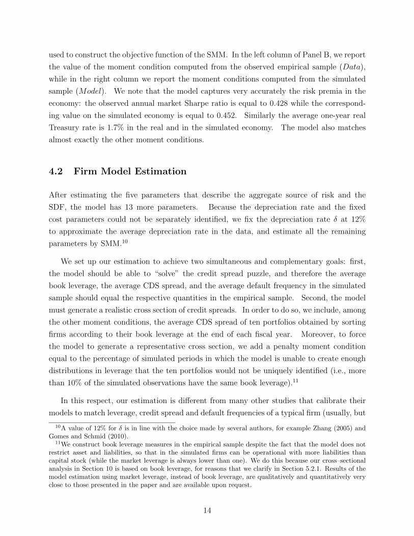
We set up our estimation to achieve two simultaneous and complementary goals: first,

the model should be able to “solve” the credit spread puzzle, and therefore the average

book leverage, the average CDS spread, and the average default frequency in the simulated

sample should equal the respective quantities in the empirical sample. Second, the model

must generate a realistic cross section of credit spreads. In order to do so, we include, among

the other moment conditions, the average CDS spread of ten portfolios obtained by sorting

firms according to their book leverage at the end of each fiscal year. Moreover, to force

the model to generate a representative cross section, we add a penalty moment condition

equal to the percentage of simulated periods in which the model is unable to create enough

distributions in leverage that the ten portfolios would not be uniquely identified (i.e., more

than 10% of the simulated observations have the same book leverage).11

In this respect, our estimation is different from many other studies that calibrate their

models to match leverage, credit spread and default frequencies of a typical firm (usually, but

10A value of 12% for δ is in line with the choice made by several authors, for example Zhang (2005) andGomes and Schmid (2010).

11We construct book leverage measures in the empirical sample despite the fact that the model does notrestrict asset and liabilities, so that in the simulated firms can be operational with more liabilities thancapital stock (while the market leverage is always lower than one). We do this because our cross–sectionalanalysis in Section 10 is based on book leverage, for reasons that we clarify in Section 5.2.1. Results of themodel estimation using market leverage, instead of book leverage, are qualitatively and quantitatively veryclose to those presented in the paper and are available upon request.

14

not exclusively, a BBB one), as for example Chen, Collin-Dufresne, and Goldstein (2009),

Chen (2010), and Kuehn and Schmid (2013). Our estimation is also different from the cal-

ibration of Bhamra, Kuehn, and Strebulaev (2010) and Arnold, Wagner, and Westermann

(2012), who impose their simulation to start from very specific points, in order to replicate

actual cross-sectional distributions of credit spreads and leverage within selected risk classes

(e.g., A, BBB, BB, B). We endogenously obtain realistic steady–state distributions of lever-

age and credit spreads that match those of a sample of real firms, for which we can observe

CDS spreads and actual default events.

4.2.1 Parameter Estimates

We present results of the estimation of the firm model in Table 2. In panel A, we report

the estimated parameters with their respective standard errors.

The autocorrelation and volatility parameters of the idiosyncratic productivity shock are

in order with what one would expect. The idiosyncratic shocks is less persistent then the

aggregate shock, 0.630 versus 0.873, and more volatile, 0.442 versus 0.010. Both parameter

estimates are statistically significant.

The estimated corporate tax rate, τ , (net of the effects of personal taxes on equity and

debt income) is 0.117 and not statistically significant. The point estimate, however, is

close to the number, 0.132, estimated by Graham (2000), and used also by Chen (2010) in

his calibration, but lower than 0.150 as in other related papers, like Bhamra, Kuehn, and

Strebulaev (2010).12

The estimated equity issuance cost, ϕ, is 0.061 and very close to the values reported by

Hennessy and Whited (2005) and Altinkilic and Hansen (2000), 0.059 and 0.051, respectively.

It is not statistically significant. The estimated debt adjustment cost parameter, θ, is 0.086

and not statistically significant. Other authors have modeled debt issuance costs as a

proportion of newly issued debt: Chen (2010) uses 0.01, Fischer, Heinkel, and Zechner

(1989), and Bhamra, Kuehn, and Strebulaev (2010) use alternatively 0.01 or 0.03. A direct

comparison to this other numbers is therefore difficult, and so is an evaluation of the relative

cost of issuing equity versus issuing debt.

The estimate for α is 0.826. In the literature there does not seem to be a very large

consensus on what the value should be. For example, Kuehn and Schmid (2013) set α

12The net tax benefit to debt estimated by Graham (2000) is 0.132 and is obtained as (1 − τD) − (1 −τC)(1− τE) = (1− 0.296)− (1− 0.350)(1− 0.120), where τE is the personal tax rate on equity flows, τD isthe personal tax rate on debt flows, and τC is the corporate tax rate.

15

to 0.65 in a model very similar to ours. However there are large bounds around those

figures: estimates for α vary between 0.30, as in Zhang (2005) to 0.75, as in Riddick and

Whited (2009).13 We obtain an estimate for the fixed cost parameter, f , equal to 0.609.

The figure is far from that used by Kuehn and Schmid (2013), 0.02 at quarterly frequency

(0.08 at annual frequency), and close to the one in Cooper (2006) who uses 0.48. Carlson,

Fisher, and Giammarino (2004) produce a much higher estimate, 1.54, although with a

different specification of the production technology. As we will discuss further the fixed cost

parameter has a key role in the ability of the model to generate a reasonable cross-sectional

distribution of leverage and credit spreads. A number as small as the one used by Kuehn

and Schmid (2013) would allow us to match average firm characteristics, as they do, but

would not allow us to generate enough dispersion in the cross section. Intuitively, this

is due to the fact that to replicate the cross-sectional characteristic of the data we need a

model with very large cash flow volatility. The three parameters most responsible for this

are σy, α and f . In our estimation, all of them are quite large. In unreported estimation

experiments, we fixed either α and/or f to the values we found in the literature, and the

fitting was extremely poor, especially on the high credit risk classes.

The estimated value of the bankruptcy cost parameter, η, is 0.499. Similar to the case

of the production function parameter, there is not a very strong consensus on what this

parameter should be. Gomes and Schmid (2010) use 0.25 (although in a specification where

the cost is proportional only to the depreciated value of the asset and there is a fixed dead

weight cost of liquidation); Hennessy and Whited (2007) estimate the parameter to be 0.104.

Glover (2012) estimates default cost parameters at the firm level (using a simpler model)

and finds an average value of 0.432, and values that range from 0.189 for lower rated firms

to 0.568 for AAA rated companies.

The estimated value of the recovery rate parameter, R, is 0.314. The estimate seems

in line with the empirical evidence presented in the literature: Glover (2012) presents an

average recovery rate equal to 0.423 based on Moody’s data; Doshi (2012) reports implied

estimates based on 5-year CDS contracts of 0.338 and 0.143, for senior and subordinated

reference obligations, respectively.

A small set of parameters does not have any direct benchmark for comparison: the invest-

ment cost parameter, λ1, is close to zero and statistically insignificant. The disinvestment

cost parameter, λ2, is estimated to be equal to 0.304, meaning that a disinvestment of 1.3

units of capital from a level of capital equal to 10 units, would cost approximately 0.420

13Gomes (2001) sets α to 0.3, Hennessy and Whited (2005) estimate a value of α equal to 0.551, whileHennessy and Whited (2007) estimate a value of 0.620. Gomes and Schmid (2010) use 0.65.

16

(30% of the disinvestment), thus leading to a cash inflow of 0.880. Finally, the distress cost

parameter, ξ, is estimated at 0.189.

It is worth pointing out that the total cost of financial distress, which plays an important

role in our paper, is not simply given by the parameter ξ, but it depends on how the firm

decides to resolve the cash short-fall. The firm has essentially two choices that are not

mutually exclusive: it can sell a portion of the asset in place (thus incurring an adjustment

cost), or it can raise equity capital (thus incurring an equity flotation cost).

Let us say that a financial loss of v < 0 is realized: if the firm chooses the first option (i.e.,

it liquidates part of the asset) the equity distribution will equal w = v(1 + ξ)− I − h(I, k),

so that the total cost of resolving the financial distress equals |v|ξ + h(I, k). If the firm

chooses the second option (i.e., raise equity), then the equity distribution becomes w =

v(ξ + ϕ+ ξϕ) < 0, and the total cost of resolving the financial distress is |v|(ξ + ξϕ).

Finally, the firm might choose to, or might have to, rely on both. In this case, the cost

of resolving financial distress is |v|(ξ +ϕ+ ξϕ) + h(I, k)(1 +ϕ) + Iϕ. In either one of those

three cases the cost of financial distress is approximately between 23% and 26% of the actual

loss.14

14To illustrate how large the impact of financial distress can be, the effect of non–linearity of the adjustmentcost with respect to the disinvestment, and the dependence of the current capital stock, assume that a firmhas a cash shortfall v = −0.1. Let’s assume that the firm may decide one of the four alternative investmentpolicies: I = 0,−0.05,−0.1,−0.15.

To begin with, assume the capital stock is low, say k = 3. If I = 0, then the actual payout will be d = −0.1and the cost −v(ξ + ϕ + ξϕ) = 0.0262, or about 26% of the cash shortfall. If I = −0.05 or I = −0.1, thecorresponding payouts will be d = v − I = −0.05 or 0 and the costs −v(ξ + ϕ+ ξϕ) + h(I, k)(1 + ϕ) + Iϕ =0.0253 and 0.0290, respectively. Finally, if the firm decides to disinvest more than needed to resolve thefinancial distress, I = −0.15, the dividend would be d = v − I = 0.05, with an associated overall cost of−vξ + h(I, k) = 0.0379. While, based on these examples, nothing can be said about the optimality of thefour policies, from a cost–minimization perspective the best is to sell asset, I = −0.05, while raising also 0.05of equity capital: this leads to an overall cost of about 25% of the cash shortfall. Thus, the examples showsthat in the model the trade-off between real and financing frictions can be non–trivial, due to the convexityof the adjustment cost function, h(I, k).

To show how the cost of resolving the financial distress is affected by the current capital stock, considerthe same example but for a larger firm, with k = 8. While the cost is independent of k if I = 0, in the othercases the cost is generally lower than for a smaller firm (k = 3). Specifically, if I = −0.05 or I = −0.1, theoverall cost −v(ξ + ϕ + ξϕ) + h(I, k)(1 + ϕ) + Iϕ = 0.0239 and 0.0234, respectively. Finally, if I = −1.5,the cost is −vξ+ h(I, k) = 0.0260. This shows that, in the model, for a larger firm, in case of insolvency ona cash flow basis, it is relatively less expensive to sell assets, at an overall cost of about 23% of the shortfall.

To fully appreciate the impact of distress costs in the model, let reconsider the above example, with k = 3,assuming that ξ = 0. In this case, holding everything else equal, for I = 0 the overall cost is 6.1% of the cashshortfall, for I = −0.05 it is 5.3%, for I = −0.1 it is 8.9%, and for I = −0.15 it is 19%. Therefore, excludingdistress costs from the model forces a much higher (and most likely unrealistic) estimates for either λ2 or ϕ.

17

4.2.2 Model Fit

In panel B of Table 2, we compare the 14 moment conditions used to construct the objective

function of the SMM: the average book leverage, the average five-year CDS spread, the

annual default frequency, the percentage of years in which the model produces enough cross-

sectional dispersion so that we are able to sort simulated observations in ten decile portfolios

(i.e., there are not more than 10% of the observations in one year that have the same book

leverage). In the left column we report the value of the moment condition computed from

the observed empirical sample (Data), while in the right column we report the moment

conditions computed from the simulated sample (Model).

Given the estimated parameters, the model is able to generate a 41.9% average book

leverage that is very close to the 43.1% observed in the data. At the same time, it produces

an average credit spread, 1.3%, and an average one-year default frequency, 0.521%, that are

also very close to the respective empirically observed quantities, 1.3% and 0.491%. The

model also produces a realistic cross section of leverage ratios almost all the times (99% of

valid sorting). The model thus achieves the first goal and is able to explain the credit-spread

puzzle.

The model is also successful on the front of generating a realistic cross section of CDS

spreads. The absolute mean pricing error of the ten leverage portfolios is equal to 6.4 basis

points, while the maximum is 12.1 basis points (the minimum is 0.1), indicating that all

portfolios are reasonably priced. Moreover, as we can observe from Figure 2, the model is

not only able to generate an upward sloping curve (higher leverage leading to higher CDS

spreads) that is in line with the empirical counterpart, but it is also able to replicate the

non-linearity between credit spreads and the highest leverage portfolios (i.e., the relation

between leverage and credit spreads is convex).

Overall, the model cannot be rejected by the data. The test of over–identifying restriction

cannot reject the null hypothesis at conventional statistical levels: the Hausman J-statistic

is equal to 4.103 with a critical value of 5.991 at the 95th confidence level (and 2 = 14 - 12

degrees of freedom).

4.2.3 Dynamic Investments versus Fixed Assets

In this section we investigate the contribution of considering dynamic investment policies to

the ability of the model to fit the data. We estimate two versions of the model in which the

firm asset is kept constant: investments are forced to be equal to the economic depreciation.

18

In the first version (Fixed Asset) of the model all firms are constrained to have the same

capital stock. In the second version (Fixed Asset Uniform) we randomly assign different

asset levels to different firms, so that firms’ capital stocks have a uniform cross–sectional

distribution in each simulated sample.

Results of the estimation exercise are presented in Table 3. In Panel A we report the

estimated parameters of the two fixed asset versions of the model and compare them to

the estimates from the basic model. In Panel B we compare the moment conditions and

report the model statistics. It is immediately obvious that the model with fixed asset has a

poor fitting: both versions are rejected by the data according to the Hausmann test. Both

versions require a higher leverage ratio to match the average credit spread, even though

they need higher bankruptcy cost and lower recovery rates, as is shown in Panel A. As

shown in Figure 3, where we display the book leverage of the ten leverage portfolios, none

of the models (the base model included) can reproduce an exact cross-sectional distribution

of leverage. All three models come relatively close in producing firms with low leverage,

but differ vastly on the opposite end, with the basic model coming the closest to producing

simulated sample that matches the right tail of the empirical leverage distribution.

The cause of the rejection by the data of the fixed asset models can be easily identified

when we consider the cross–sectional distribution of CDS spreads. As was pointed out by

Huang and Huang (2003), traditional structural models fail to be able to generate enough

credit risk for firms with very good credit rating. Similarly in our estimation exercise we

find that the model with static assets is not able to generate sufficient levels of CDS spreads

for top 30% of the firm in credit standing (low leverage firms). As a result, although the

average CDS spread is very close to average in the empirical sample, the cross–sectional

average pricing error (across all ten portfolio) is relatively large for both version of the fixed

asset model. Finally, only the version with uniformly distributed asset across firms is able

to generate enough dispersion in the simulated sample to create the ten leverage portfolios.

In summary, allowing for dynamic investments gives the model the ability to not only

match the unconditional moments, but also to generate a better cross-sectional distribution

of leverage, as suggested by Leary and Roberts (2005) and Hennessy and Whited (2005),

and credit spreads.

4.2.4 Robustness Checks: One-year CDS Contracts

In the main estimation procedure we have decided to estimate the model’s parameters using

a 5-year maturity (tenor) for the reference CDS contract. This choice is entirely driven by

19

the fact that these contracts are the most liquid and therefore guarantee a large number

of observations. A larger number of observation guarantees less noise in the estimation of

the averages and covariances of the empirical moments. Similarly, since later in the paper

we intend to cross–validate the model by running standard regressions where the dependent

variable is the CDS spread, it is important that we have as many observations as possible.

Nonetheless, the model’s underlying security is a one-year bond and, as we noted in

Section 2.4, the prices of CDS contracts are obtained by keeping fixed the firm’s policy. It

would seem natural to estimate the model’s parameters by pricing one-year CDS contracts,

as opposed to five year ones.

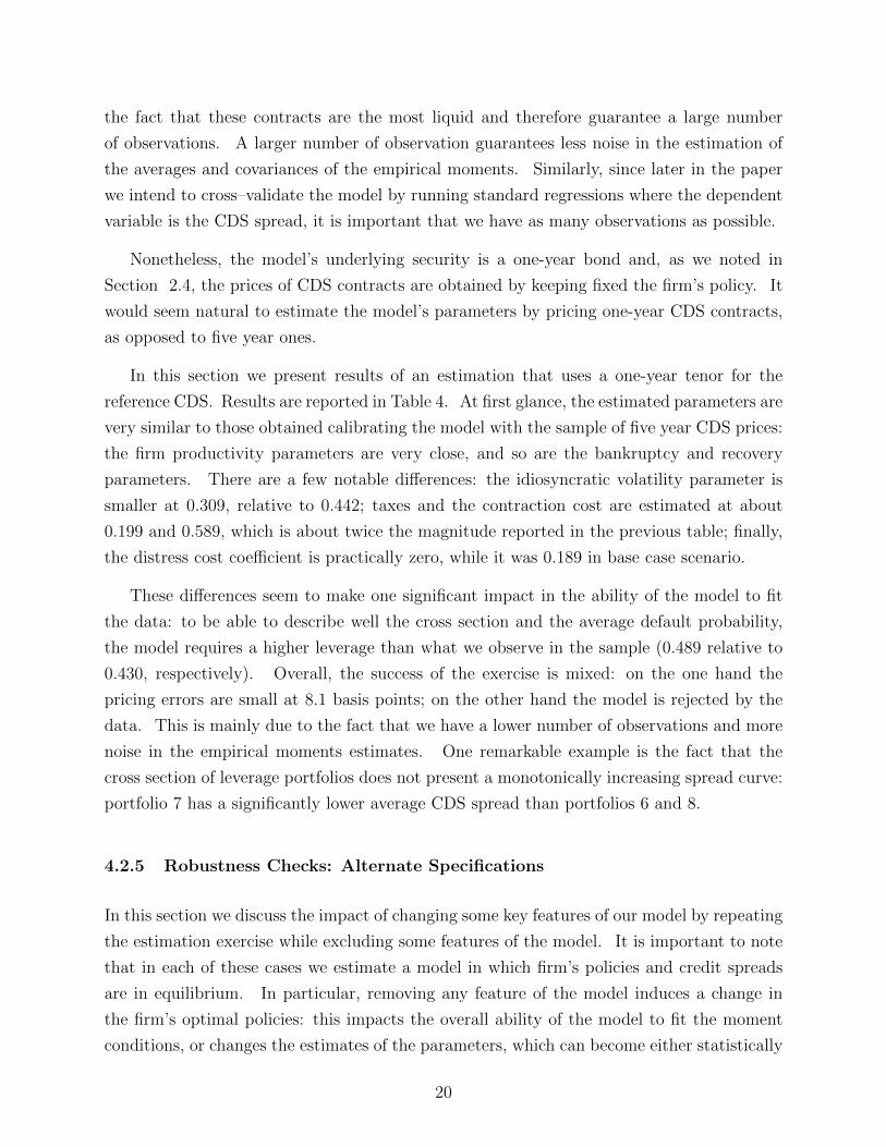
In this section we present results of an estimation that uses a one-year tenor for the

reference CDS. Results are reported in Table 4. At first glance, the estimated parameters are

very similar to those obtained calibrating the model with the sample of five year CDS prices:

the firm productivity parameters are very close, and so are the bankruptcy and recovery

parameters. There are a few notable differences: the idiosyncratic volatility parameter is

smaller at 0.309, relative to 0.442; taxes and the contraction cost are estimated at about

0.199 and 0.589, which is about twice the magnitude reported in the previous table; finally,

the distress cost coefficient is practically zero, while it was 0.189 in base case scenario.

These differences seem to make one significant impact in the ability of the model to fit

the data: to be able to describe well the cross section and the average default probability,

the model requires a higher leverage than what we observe in the sample (0.489 relative to

0.430, respectively). Overall, the success of the exercise is mixed: on the one hand the

pricing errors are small at 8.1 basis points; on the other hand the model is rejected by the

data. This is mainly due to the fact that we have a lower number of observations and more

noise in the empirical moments estimates. One remarkable example is the fact that the

cross section of leverage portfolios does not present a monotonically increasing spread curve:

portfolio 7 has a significantly lower average CDS spread than portfolios 6 and 8.

4.2.5 Robustness Checks: Alternate Specifications

In this section we discuss the impact of changing some key features of our model by repeating

the estimation exercise while excluding some features of the model. It is important to note

that in each of these cases we estimate a model in which firm’s policies and credit spreads

are in equilibrium. In particular, removing any feature of the model induces a change in

the firm’s optimal policies: this impacts the overall ability of the model to fit the moment

conditions, or changes the estimates of the parameters, which can become either statistically

20

insignificant or economically implausible.

We will focus on four key features of the model: the presence of distress costs, ξ; the

role of fixed costs, f ; the impact of real adjustment costs, λ1 and λ2; the role of financing

frictions, in the form of equity floatation costs, ϕ, and debt adjustment costs, θ. The results

of the five estimation exercises are reported in Table 5.

In the first alternate specification, we exclude financial distress costs (and therefore the

state of financial distress) by setting ξ equal to zero. The goodness of fit of this model is

lower than the base case scenario and the model is now rejected by the data: this is mainly

due to the fact that this specification produces a higher average leverage than the one found

in the data or in the base case model, and diminished ability of the model to create cross-

sectional heterogeneity. In economic terms, eliminating the financial distress cost channel

leads to the amplification of other cost channels: higher taxes (almost double) and higher

capital adjustment costs (again almost double the base case parameters). Also this is the

only variant of the model in which the debt adjustment costs appear to be statistically

significant.

The second variation on the model is given by the exclusion of fixed costs from the

determination of the firm’s cash flow, i.e., we set f equal to zero. Interestingly the ability of

the model to create cross-sectional heterogeneity is directly linked to the operating leverage.

Without fixed costs, the model is completely unable to create dispersion among firms, a

feat that is achieved in less than 8% of the simulated years. Similarly to the previous

case, after eliminating one of the principal cost component in the estimation exercise, other

costs increase: taxes, distress costs, and cost of contraction. Notably the estimation also

returns a much higher degree of autocorrelation for the idiosyncratic productivity process.

In summary, the model is rejected by the data.

In the third specification we suppress the capital adjustment costs, λ1 and λ2. Note

that the expansion costs was not economically or statistically important in the base case

scenario, so that the real change here is the elimination of the contraction cost. Regardless,

this changes the ability of the model to fit the data. The model is in fact statistically

rejected by the data, and it produces higher leverage, credit spreads and default probabilities.

Surprisingly the elimination of the contraction cost does not lead to an increase of the distress

cost (the parameter is in fact much smaller). Even more surprisingly, this leads the model

to produce higher leverage, credit spreads and default frequency.

The fourth and final alternative specification is characterized by the absence of issuance

costs, as both the equity floatation cost and the debt adjustment costs parameters are set

21

to zero. Not surprisingly, since those estimates were not statistically significant in the base

case scenario, this variant of the model is the one that comes closer to the base case.

What we learn from this exercise is that not all trade-offs are equally important in terms

of their ability to help the model to match the cross-sectional features of the data. Clearly,

the operating leverage plays a big role in this type of models. Asset adjustment costs seem

relevant only when it comes to contraction, while expansion costs do not seem to be that

crucial. Also, equity issuance costs and debt adjustment costs do not appear to be key

ingredients of a successful model. On the other hand, some of these features might be more

important for a model focused at capturing time-series dynamics (i.e., financial frictions help

explain some path dependencies that can be observed in the data).

4.2.6 Robustness Checks: Subsamples

In this section we discuss the impact of considering different aggregate economic conditions.

We repeat the estimation exercise separately for the years 2003-2006 and for the years 2007-

2010, thus separating the sample in two periods: one that contains the crisis and one that

does not. Because the performance of firms during the second period is heavily conditioned

by the economic crisis of 2007-2008, this experiment should give us a good understanding of

the ability of the model to adapt to different conditions.

We report results of these estimation in Table 6. From Panel A, we note that some

of the parameters are different across the two estimations. The autocorrelation of the

idiosyncratic productivity shock is higher in the non-crisis period while the opposite is true

for the volatility parameter. Thus, the estimation procedure is able to identify aggregate

economic conditions by adjusting the parameters of the idiosyncratic productivity shock.

On the firm front the tax-parameter is higher in the pre-crisis period, signaling a higher

benefit of holding debt when the economic environment is favorable. The parameters that

represent adjustment costs to the financing policy (through debt or equity) are instead higher

in the crisis period, as one could expect. The cost of expansion parameter is higher and

significant in the pre-crisis period. The fix cost and the distress cost parameters are also

higher in the crisis period, indicating that the firms operations appear riskier in an economic

downturn. Finally, while the bankruptcy cost remains virtually unchanged, the recovery

rate on par is much higher in the crisis period than it is in the more tranquil time.

From Panel B, we note that the overall ability of the model to match the moment con-

ditions is relatively good in both sub–periods. In both periods the model does an accurate

22

job at capturing the average leverage and credit spread. Possibly the only dimension in

which the model has difficulty reconciling the data is the default frequency: the model

over–estimates the default frequency in the crisis period by a significant amount.

Overall, in both sub-periods, the model is again not rejected by the data. This seems

particularly noteworthy given the relatively large average pricing error in the crisis-period,

when the cross section of credit spreads is particularly steep relative to leverage.

5 CDS Spreads and Firm Policies

The results described in the previous section, which are produced using variation in leverage

as a source of conditional information, outlines the importance of considering variation in

asset dynamics in characterizing the cross-sectional distribution of credit spreads. The

past, current, and future investment choices are expected to impact credit risk because of

two key aspects of the model. First, firm’s profitability, because of mean-reversion in the

productivity shocks, exhibits persistence. Second, the firm incurs asymmetric adjustment

costs to the capital stock. While in good states of the world, the option to grow (i.e., making

investments in the future) is valuable as it is indicative of future profitability and solvency,

in bad states of the world, having not realized the option to grow is valuable as it spares the

possible large downsizing costs.

Following Hennessy and Whited (2005), as an “out–of–sample” test of the model, we

study how variation in credit spreads is associated to observable characteristics that are

a direct consequence, in the model, of dynamic choices that firms make about their asset

structure. We concentrate on the firm’s actual production capacity and cost structure

(operating leverage), on the prospects for the future production capacity (growth options)

and on the realization of these prospects (investments). We investigate these relationships

by juxtaposing a sample of empirically observed firms to a simulated economy.

5.1 Operating leverage and credit spreads

In this section, we examine the relation between credit risk and operating leverage (i.e., the

volatility of cash flow related to the incidence of fixed costs). Because of restrictions in

the functional form of the production function, we adopt a particular definition of operating

23

leverage at the end of period ]t− 1, t] as the ratio of fixed production costs to EBITDA

OPL(s, p) =ex+zkα − π(s, k)

π(s, k)=

fk

π(s, k). (11)

The equivalent to equation (11) in the observed data is given by the difference between sales

and EBITDA, over EBITDA.15

While we model insolvency both from a value and a cash flow perspective, operating

leverage is an important determinant of credit risk from a cash flow perspective. Everything

else equal, large fixed costs make the firm more likely to be insolvent on a cash flow basis in

a downturn, thus reducing the firm ability to meet the debt obligations.

In Table 7 we report results of panel regressions of 5-year CDS spreads on book leverage

and operating leverage. In the first two columns, labeled Data, we report results obtained

from the empirical sample. In columns (3) and (4), labeled Model, we report results

obtained from the simulated sample. This last set of results is obtained by estimating the

regression parameters for each of the 50 simulated samples. The reported parameters are

then computed by averaging across the 50 estimations. Similarly, the standard error of

each parameter is obtained as the standard deviation of the 50 parameter estimates. All

regressions include time fixed effects. The regressions based on the Data sample also include

industry fixed effects, and have standard errors clustered at firm level.

As we can see from columns (1) and (3), controlling for book leverage, operating leverage

has a positive and statistically significant coefficient. High fixed costs, and in general a

large overhead, increase the likelihood of having insufficient funds to service the debt if a

bad scenario occurs. The estimated coefficient on the interaction term between book and

operating leverage, columns (2) and (4), is not statistically significant.

A similar perspective can be obtained from independent quartile sorting of CDS spreads

by book leverage and operating leverage. In Panel A of Table 8 we report results obtained

from the empirically observed data (Data), while in Panel B we report results for the simu-

lated sample (Model). For all the leverage quartiles, there is a positive relationship between

credit spreads and operating leverage. As evidenced in Panel A and consistent with the sign

of the interaction variable in the regression model, the relation becomes stronger for higher

leverage.

15Note that this is partly at odds with conventional definitions of operating leverage (percentage changeof sales divided by percentage change of EBITDA), which are generally estimated in a regression approach.Unavailability of a long time series for the observed data precludes us from following this traditional approach.

24

5.2 Growth options and credit spreads

In this section, we discuss the relation between credit risk and growth opportunities. In the

context of our model, this relation can be easily understood by observing Figure 4. There

are two basic mechanisms that generate growth options: persistency of firm specific shocks

and decreasing return to scale. The first mechanism can be highlighted by considering, at a

particular date, two firms with the same ratio of debt to asset in place (i.e., the same book

leverage) and the same capital stock. Let’s assume that the first firm has just observed a

positive realization while the second has observed a negative realization of the idiosyncratic

shock. The first firm has higher growth options than the second one. Because the shocks

are persistent, the option to grow is due to the fact that the firm is on a high trajectory of

the firm specific shock, and therefore expects also a positive shock in the next period. If

that shock is large enough the firm might decide to invest (the decision to invest will also

depend on the realization of the aggregate shock).

We illustrate the second mechanism also with an example. We now consider two firms

with the same leverage but different levels of capital stock (i.e., different size, as measured by

the book value of the assets). Let’s assume that both firms observe a positive idiosyncratic

shock. The future prospects of the two firms are not the same. In fact, because the

production function exhibits decreasing return to scale, the smaller firm has better future

prospects and hence more growth options.16

In summary, cross-sectional differences in growth options for firms with the same lever-

age arise because firms have different capital in place and/or because they are on different

trajectories of the firm specific shock. Because of that, some firms find themselves in a

situation in which they expect to be very profitable in the future.

The relation between credit risk and growth options can now be easily formalized. With

one period debt, investments and debt repayment are contextual (i.e., the two decision are

simultaneous). Since growth options signal the ability of the firm to make future investments

because of the expected future profitability, they also signal the expected ability of the firm

to repay current debt. Accordingly, after controlling for book leverage, the relation between

credit spread and growth options should be negative.

In Table 9 we present the estimation results of panel regressions of 5-year CDS spreads on

book leverage and market–to–book, or Q for short, ratio. In the first two columns, labeled

Data, we report results obtained from the empirical sample. In columns (3) and (4), labeled

16This effect is what is reproduced also by Carlson, Fisher, and Giammarino (2004) in their model.

25

Model, we report results obtained from the simulated sample. This last set of results is

obtained by estimating the regression parameters for each of the 50 simulated samples. The

reported parameters are then computed by averaging across the 50 estimations. Similarly,

the standard error of each parameter is obtained as the standard deviation of the 50 parame-

ter estimates. All regressions include time fixed effects. The regressions based on the Data

sample also include industry fixed effects, and have standard errors clustered at firm level.

As we can see from columns (1) and (3), controlling for book leverage, the Q–ratio has

a negative and statistically significant coefficient. While the relation between CDS spreads

and market–to–book is on average negative, it is not obviously negative for all levels of

leverage. We include an interaction term between leverage and market–to–book in columns

(2) and (4). The estimated coefficient on the interaction term suggests that the relation is

more pronounced for high leverage firms, while it is at best very weak for low leverage firms.

A similar perspective can be obtained from independent quartile sorting of CDS spreads

on book leverage and market–to–book. In Panel A of Table 10 we report results obtained

from the empirically observed data (Data), while in Panel B we report results for the simu-

lated sample (Model). The sorting procedure in the case of the simulated sample involves

first sorting in each time period of each one of the 50 simulated samples. Next, we av-

erage across time. Finally, the results reported are obtained by averaging across the 50

simulated samples. For all the leverage quartiles, there is a negative relationship between

credit spreads and market–to–book ratio. As evidenced in Panel A and consistent with the

significance of the interaction variable in the regression model, the relation becomes stronger

for higher leverage. We find a similar pattern in the simulated sample, Panel B, with the

exception of the highest leverage quartile for which the credit spread reduction is less marked

(this portfolio is not very well populated).

The model allows us to interpret the negative and statistically significant interaction term

between market to book ratio and book leverage in terms of insolvency on a cash flow basis.

A high market to book ratio proxies for a high expected future cash flow (or profitability)

and this is more beneficial for firms with more debt, in terms of their ability to meet financial

obligations. On the contrary, firms that do not have much debt, do not need high future

cash flows to meet their obligations.

The economic forces that generate the negative relation between credit spreads and

market–to–book ratios are the autocorrelation of the idiosyncratic productivity shocks and

the curvature of the production function. A higher autocorrelation coefficient and a pro-

duction function that exhibits decreasing returns to scale at a higher degree (smaller α),

26

ought to make the relation between credit spreads and market–to–book ratios stronger, thus

producing more negative regression coefficients.

In the spirit of Riddick and Whited (2009), we investigate those premises by conducting

sensitivities of the regression coefficient by estimating additional regressions of CDS spreads

on leverage and market–to–book ratios in simulated samples obtained by changing the model

parameters of interest. Each sample is obtained by simulating the model with the set of

estimated parameters reported in Table 2, but perturbing the autocorrelation of the idiosyn-

cratic shock (ρz) and the production function parameter (α) in the interval [−0.05, 0.05]

around the estimates reported in Table 2, ρz = 0.630 and α = 0.826. Because changing

the optimal parameters produces more skewed samples, we standardize all variables before

estimation. The results of these analyses, which are reported in Table 11, validate our con-

jectures: the regression coefficient on the market–to–book ratio is more negative in samples

with higher ρz and lower α.

Notably, the reported negative conditional correlation between credit spreads and market–

to–book ratios is apparently in contrast with the predictions of the theoretical models pro-

posed by Arnold, Wagner, and Westermann (2012) and the calibration results presented by

Kuehn and Schmid (2013). Although the predictions of our model line up with the empirical

evidence, some discussion is required.

In the rest of this section, we make a few considerations about some of the most troubled

economic hinges on which the relation between credit risk and growth options rests. First,

we explore two issues that make the relation between credit spreads and market to book ratio

difficult to interpret as equivalent to the relationship between growth options and credit risk:

we discuss the choice of book and market leverage as the proper control in a regression of

credit spreads on growth options. Moreover, we investigate the information content of the

market to book ratio as a proxy for growth options, and try to distinguish the value of the

options to grow from the value of the assets in place. Second, we borrow from the framework

in Arnold, Wagner, and Westermann (2012), and discuss the relative impact of distinct value

channels that affect growth options.

5.2.1 Growth options, book and market leverage

The relation between credit spreads and the market to book ratio is affected by the choice

of which leverage measure is used in the regression. For example, including (quasi) market

leverage instead of book leverage in Table 9 would lead the parameter of the market to

book ratio to switch sign (from negative to positive), as for example reported by Kuehn and

27

Schmid (2013).

Both signs are theoretically possible as the following example illustrates. Consider

two firms, denoted 1 and 2, with the same book leverage, b′1/k′1 = b′2/k

′2, and different

market to book ratio, b′1/k′1 + S1/k

′1 > b′2/k

′2 + S2/k

′2. Using the first equality, the second

condition can be rewritten S1/k′1 > S2/k

′2, which suggests that the firm with higher market

to book ratio has relatively higher equity valuation and better prospects. Since those

are negatively related to the probability that the firm has financial problems, it leads to a

negative correlation between credit spreads (risk) and market to book ratios. This is what

we find in our analysis.

Consider now two firms with the same quasi–market leverage b′1/(b′1+S1) = b′2/(b

′2+S2), or

after some manipulations S1/b′1 = S2/b

′2. The two firms have different market to book ratio,

b′1/k′1+S1/k

′1 > b′2/k

′2+S2/k

′2, or equivalently (1+S1/b

′1)b′1/k

′1 > (1+S2/b

′2)b′2/k

′2. After using

the quasi-market leverage equality, the last inequality can be rewritten as b′1/k′1 > b′2/k

′2.

What we learn is that, fixing the quasi-market leverage, the firm with higher market to

book ratio has higher book leverage and therefore higher credit risk. Therefore, controlling

for quasi-market leverage, the correlation between credit spreads and market to book ratio

should be positive. This is what Kuehn and Schmid (2013) find.

We conclude that controlling for market leverage might lead to a problematic interpre-

tation of the sign of the market to book ratio coefficient in a regression of credit spreads.

5.2.2 Market to book ratio, options to grow and asset in place

The relation between credit spreads and market to book ratio is also affected by the fact that

the market to book ratio contains information about the firm that is not directly related to

growth options. We explore this issue in this section.

In the model, a growth opportunity is the option to build additional production capacity

through investments. In order to measure the value created by growth options, we first

determine the value of the equity when the firm follows the optimal policy p∗ = (k∗, b∗) =

F (s, p) subject to the constraint that it cannot increase the production capacity. We define

Sng (equity with no–growth) as the fixed point of the following functional equation

Sng(s, p) = max 0, dng + Es [M(s, s′)Sng(s′, p′)] , (12)

where p′ = (k′, b′) = (k∗, b∗) if k∗ ≤ k, and (k′, b′) = (k, b∗) if k∗ > k. Because Sng is

obtained from S by imposing a stationary sub–optimal policy, the value of the equity in the

28

case of no-growth, Sng, is strictly less than the optimal value of the equity, S. The difference

between S and Sng has two components: the first originates from the effect of the inability

to grow (i.e., the current investment policy) on the dividend, which will be different from the

optimal dividend, d− dng. The second component originates from the effect of the inability

to grow on the continuation value, which in essence is the value of the growth opportunities

(i.e., the ability to increase k in the future).

The definition of Sng allows us to decompose the total firm value into three parts: b′+S =

b′ + Sng + (S − Sng): the value of the debt, the present value of the asset in place, Sng, and

the present value of growth opportunities, (S − Sng).

Thus, the market to book value can also be decomposed into three parts:

Q =(b′ + S)

k′=b′

k′+ PVAP + PVGO . (13)

where b′/k′ is the book leverage; PVAP is the present value of the asset in place, which

includes the option to liquidate part of the capital stock and the option to default, scaled by

the book value of asset, Sng/k′; PVGO is the present value of growth opportunities scaled

by the book value of asset, (S − Sng)/k′.

From Equation (13) we can see that the market to book ratio contains information not

only about growth options, but also about the firm’s credit riskiness. The decomposition

suggests that the use of the market to book ratio as a measure of growth options is feasible

only after netting out the effect of book leverage as a proxy for credit risk. However, even

after controlling for book leverage, there is still an issue that the negative relation between

credit spreads and the market to book ratio could be attributed to the value of the asset in

place, rather than to the growth options.

Unfortunately, this particular ambivalence cannot be resolved within the context of the

observed data, as it is impossible to exactly disentangle the value of the asset in place from the

value of the growth opportunities.17 We therefore defer to the simulated sample. Table 12

shows the estimation results of panel regressions that include as independent variables the

present value of the asset in place, PVAP, and the present value of the growth opportunities,

PVGO, as defined above. The results reported in the table suggest a negative relation of

credit spreads with PVAP (column 1), PVGO (column 2), and PVAP and PVGO together

(column 3). Interestingly, when all three are included PVAP, PVGO, and market to book

(after excluding book leverage) the sign of the coefficient in front of the market to book ratio

17Arnold, Wagner, and Westermann (2012) and Davidenko and Strebulaev (2007) includes R&D expen-diture as control for growth options in an attempt to get around the problem.

29

becomes positive (column 5), confirming that after removing PVAP and PVGO, the ratio

contains information related to the credit risk of the firm.

5.2.3 Volatility effect versus value effect

Simplifying the terms of the argument for sake of brevity (a much better description of the

following reasoning can be found in Arnold, Wagner, and Westermann (2012)), the option

to grow matters to bond holders only in downturns, because that is when their cash flows

are affected by company decisions. In a downturn, the cash flow volatility of the firm goes

up and that increases the value of the growth option. This is known as volatility effect.

At the same time, because risk premia are countercyclical, an economic downturn de-

creases the value of future cash flows. This decreases the value of the option to grow,

because the underlying asset is less valuable. This is known as value effect.

The sign of the relation between credit spreads and growth options is therefore dictated

by which one of these two effects is prevalent. Obviously, anyone of those two effects can

become prevalent depending on the model calibration.

Although in our setting these effects are not explicit, they are nevertheless at play. So one

simple reconciliation of the theoretical result proposed by Arnold, Wagner, and Westermann

(2012) and the results reported in Table 9, is that in their model’s calibration the value effect

is more prominent, while in the empirical sample that we examine, and consequently in our

model’s calibration, the volatility effect prevails.

5.3 Path dependency, investments and credit spreads

The model is characterized by path dependencies of the policies. At any period, in fact, the

firm’s optimal policies (investment, debt issuance and equity distributions) depend on the

asset and debt choices that the firm made in the previous period. Consequently, both the

firm’s leverage and the firm’s credit spread exhibit path dependency.

This particular aspect of the model has been neglected in the discussions presented in the

previous sections. We analyze it here. Path dependency in the policies has two important

consequences for our analysis of credit spreads. First current credit spreads should also

depend on past choices of debt and capital. Second, changes in credit spreads should be

associated with changes in the policies (i.e., changes in capital and changes in debt). We

analyze those two possible economic determinants of credit spreads separately.

30

In Table 13, we report panel regressions of 5-year CDS spreads on current and lagged log

levels of asset size and debt amount. In the left panel, labeled Data, we report results for the

observed data. In the right panel we report results based on the simulated economy, Model.

The results reported in Columns (2) and (5) show that, after controlling for the expectations

of future cash flows through the market to book ratio, credit spreads are negatively correlated

with the contemporaneous asset level and positively correlated with the contemporaneous

debt level. This is equivalent to what we find in Columns (1) and (4), that the credit spreads

(respectively, empirically and in the model) are positively correlated with book leverage.

Absent financing and real frictions, the new level of asset and debt would depend only

on the realized shocks. However, because adjustments are costly, the chosen levels of asset

and debt depend also on their respective lagged values. In other words, firms with the same

current leverage, b′/k′, and that are exposed to the same shocks may have different credit

spreads according to what their respective previous levels of asset and debt were. Column

(3) and (6) of Table 13 show that credit spreads are negatively related to current assets and

positively related to lagged assets. Similarly credit spreads are positively related to current

debt and negatively related to lagged debt.

In Table 14 we report regression results of changes in CDS spreads on several firm char-

acteristics. In columns (1) and (3) we consider changes in leverage. As should be expected,

changes in leverage and changes in credit spreads are positively related. In column (4) we

decompose the changes in leverage between changes in debt and changes in assets. Note

that because the adjustment costs to the asset are asymmetric (i.e., it costs more to disinvest

than it does to invest) the impact of an asset change on credit spreads is not symmetric.

The amount by which disinvestments increase credit spreads is much larger than the amount

by which investments decrease credit spreads. The investment and disinvestment coeffi-

cients are different also in column (2), confirming that investment adjustment costs are an

important determinant of the credit risk of a company.

6 Conclusion

We develop a structural model of credit risk that allows for dynamic investment and financing

policies, and that features financing and real frictions. Heterogeneity among firms generated

by endogenous investments is a central aspect of the model and it enables us to study the

cross-sectional relationship between credit risk and the economic forces that drive firms in

the economy. The model is structurally estimated to capture the empirical cross section of

31

credit spreads, an important aspect to solve the credit spread puzzle.

Our estimation exercise shows that current leverage, although important, is not the only

driver of credit risk, as this depends on a number of firm characteristics. Because firms

policies are path dependent and because exogenous productivity shocks are persistent, the

past and the future investment decisions also matter: current credit spreads are related to

current and past values of capital stock and debt, as well as the future economic prospects

of the firm (growth options). When the firm realizes the option to grow, by investing in

production capacity, its credit standing improves.

32

Appendix

A Proof of existence of the solution of the model

The proof of the existence of the solution S of the functional equation (3) (together with the

optimal policy F ), subject to the constraints for D in equations (5) and for PI (6) mostly

follows standard arguments by Stokey and Lucas (1989).

It is easy to prove that the choice set of the program in (3) is compact. As for k′, given

the current capital stock k, the firm cannot sell more than the current capital, or k′ ≥ 0,

and it makes no economic sense to invest more than k, such that π(x, z, k)− δk = 0, given

the strict concavity of the production function, and x and z are the best possible outcomes

for the systematic and the idiosyncratic shock, respectively.

Quite naturally, b′ ≥ 0. On the other hand, there is an upper bound for b′, say b, because

there is a tradeoff between the positive effect that increasing the debt has on current year

dividend (v, in equation (1), is increasing in both D and PI, and they are increasing in b′,

although at a decreasing rate), and the negative effect that it has on next year expected

dividend (v is decreasing in b), and this effect is magnified by a factor (1 + ξ) if the after–tax

cash flow is negative (which is the case if the debt is high), and by a factor 1 + φ if the net

proceed from selling capital is insufficient. So, we may conclude that the choice set for k′

and b′ is compact. Then, we have the following

Lemma 1. Under the stated conditions that the decision set is compact, Q has the Feller

property, M is continuous, and ω is almost everywhere continuous, the functions D and PI

are continuous in (s, p′).

To prove this result, we focus on D, as the same argument carries over to PI. In

particular, we have to show that D(s, p′) =∫u(s′, p′)M(s, s′)Q(s, ds′) is continuous. By

separating the two components of the payoff function u, this boils down to proving that

the function∫ω(s′, p′)M(s, s′)Q(s, ds′) is continuous in (s, p′), where ω(s′, p′) is the default

indicator function, which is bounded and is almost everywhere continuous (i.e., the set of

the discontinuity points has zero measure). If this is true, then D is continuous because it

is a linear combination of continuous functions.

For notational convenience, let define H(s, s′) = M(s, s′)Q(s, s′). Because M is con-

tinuous and the support of s and s′ is compact, M is bounded. We need to prove that

f(s, p′) =∫ω(s′, p′)H(s, ds′) is continuous. Of course, M does not create any concerns in

33

this respect, given Q has the Feller property (see Lemma 9.5 in Stokey and Lucas (1989)).

Because the state space is compact, there is a sequence (sn, p′n) converging to (s, p′). We

just need to prove that |f(sn, p′n)− f(s, p′)| converges to zero for n→∞. We observe that

|f(sn, p′n)− f(s, p′)| ≤ |f(sn, p

′n)− f(s, p′n)|+ |f(s, p′n)− f(s, p′)|. (14)

As for the second component in the right–hand–side of (14), we have

|f(s, p′n)− f(s, p′)| =∣∣∣∣∫ ω(s′, p′n)H(s, ds′)−

∫ω(s′, p′)H(s, ds′)

∣∣∣∣≤∫|ω(s′, p′n)− ω(s′, p′)|H(s, ds′).

By separating the support of s′ into the subset in which ω is continuous from the subset

in which it is discontinuous, |ω(s′, p′n)− ω(s′, p′)| converges to zero for n → ∞ when in the

first subset. In the second subset, the behavior of ω is not important because it has zero

measure.

As for the first component in (14),

|f(sn, p′n)− f(s, p′n)| =

∣∣∣∣∫ ω(s′, p′n)H(sn, ds′)−

∫ω(s′, p′n)H(s, ds′)

∣∣∣∣≤∫ω(s′, p′n) |M(sn, s

′)Q(sn, ds′)−M(s, s′)Q(s, ds′)| ≤M

∫ω(s′, p′n) |Q(sn, ds

′)−Q(s, ds′)| ,

where M is the maximum value of M .

Because Q has the Feller property, then it is continuous in the first argument. This can

be proved by contradiction: Assume that Q is discontinuous in s. Then, for an arbitrary

continuous function g, the function G(s) =∫g(s′)Q(s, ds′) would be discontinuous in s.

Therefore, |Q(sn, ds′)−Q(s, ds′)| converges to zero for n → ∞, and this concludes the

proof of the lemma.

Proposition 2. There is a unique solution S to the program in equations (3), (5), and (6).

S is increasing in s = (x, z) and k, and is decreasing in b.

To prove this proposition, define the operator T as follows:

(TS)(s, p) = max

0,max

p′d(s, p, p′) + βEs [m(s, s′)S(s′, p′)]

,

34

where we have specified M(s, s′) = βm(s, s′), with β < 1, so that the risk-free component of

the stochastic discount factor is highlighted.18

First, we will prove that if S is a continuous function on the compact set for (s, p), also

TS is continuous on the same compact set. Second, we will show that S1 ≤ S2 implies

TS1 ≤ TS2. Third, we will show that for any a ≥ 0, T (S + a) ≤ TS + βa. Then, because

the last two are the Blackwell sufficient conditions, if the operator T satisfies them it is a

contraction and the fixed point exists and is unique because the set of continuous functions

equipped with the sup-norm is a complete metric space.

We first show that (TS)(s, p) is continuous for all (s, p). From Lemma 1, both D and

PI are continuous. Therefore, v, w and d in (2) are continuous. Because the feasible set for

p′ is compact, using the Maximum Theorem (see Theorem 3.6 in Stokey and Lucas (1989))

the function

L(s, p) = maxp′d(s, p, p′) + Es [M(s, s′)S(s′, p′)] , (15)

is continuous. Because (TS)(s, p) = max 0, L(s, p), also TS is continuous.

As for monotonicity of the operator T , let S1 and S2 such that S1(s, p) ≤ S2(s, p) for all

(s, p). Then the following is straightforward:

(TS1)(s, p) = max

0,max

p′d(s, p, p′) + Es [M(s, s′)S1(s

′, p′)]

≤ max

0,max

p′d(s, p, p′) + Es [M(s, s′)S1(s

′, p′)]

= (TS2)(s, p).

Lastly, let

[T (S + a)](s, p) = max

0,max

p′d(s, p, p′) + βEs [m(s, s′) (S(s′, p′) + a)]

= max

0,max

p′d(s, p, p′) + βEs [m(s, s′)S(s′, p′)]+ βa

≤ max

0,max

p′d(s, p, p′) + βEs [m(s, s′)S(s′, p′)]

+ βa

= (TS)(s, p) + βa.

Monotonicity of S with respect to s = (x, z) is due to strict monotonicity of both π

and Q with respect to x and z. Monotonicity of S with respect to k and b is based on

18The fact that M is bounded make this assumption harmless.

35

monotonicity of d in equation (2) with respect to these variables. This concludes the proof

of the proposition.

Finally, the fact that the default indicator function, which has values in 0, 1, is dis-

continuous only in a set with zero measure can be proved by observing that the change of

value from 0 to 1 occurs where the continuous and strictly monotonic function L, defined

in equation (15), is equal to zero. L is strictly monotonic because S is monotonic, Q is

monotonic and π is strictly monotonic.

B Numerical procedure

The solution to the Bellman equation (3) with the constraints in equations (5) and (6),

and the related optimal policy is obtained by discretizing the state space of s = (x, z) and

the control variables p = (k, b). Because the stochastic process of systematic risk is quite

persistent we discretize the two exogenous processes using the numerical approach proposed

by Rouwenhorst (1995). x is discretized with 11 points and z with 11. The discretized set

of values for capital stock is kj = ku(1− d)j | j = 1, . . . , Nk, and the set of discrete debt

levels isbj = j bu

Nb| j = 1, . . . , Nb

with Nk = 25 and Nb = 21. The fixed point of the

Bellman equation, S, is found using a value function iteration algorithm, and the algorithm

is halted when the maximum change of value on S between two iteration is below the

tolerance 10−5. The simulated economy is composed of 50 different samples, characterized

by different histories of the aggregate state variable. Each sample is composed by a panel

of 300 independent firms, which are characterized by different histories of the idiosyncratic

variable. To make the simulated economy comparable to the observed data, each firm’s

history, after the first 20 periods are discarded, is composed by 10 periods. The desired

quantities are obtained by applying the optimal policy at each step. If a company defaults

at a given step, it is restarted at the steady state for k and b one step later.

C CDS spread

The CDS spread in equation (7) is calculated within our model as follows.

Defining H(s, s′) = Q(s, s′)M(s, s′), the product of the transition probability and the

stochastic discount factor, and given the state dependent default policy ω, we can define Hd,

the matrix of prices (using the discretized version of the transition function) of contingent

36

claims that pay one unit if we have a transition from a non–default state to a default state

in one period, and Hnd, the matrix of prices of contingent claim that pay one unit if there is

a transition from a non–default state to a non–default state.

Using a matrix notation, we define Pi = H i−1nd HdId and Si = H i

ndInd, where Id is a column

vector of ones with as many components as the number of default states, and Ind is a column

vector of ones with as many components as the number of non–default states. Then, the

credit spread is

cds = (1−R)

∑Ti=1Pi∑T

i=1 (Pi + Si)

D Estimation method

The model is estimated in two steps using the Simulated Method of Moments (SMM) of

Gourieroux, Monfort, and Renault (1993) and Gourieroux and Monfort (1996). First we es-

timate the parameters of the stochastic discount factor by matching some aggregate moment

conditions: the average and standard deviation of the aggregate Sharpe ratio, the average,

standard deviation, and first difference autocorrelation of the one year real risk free rate

(i.e., one year constant maturity Treasury rate). Second, we estimate the parameters of the

firm’s model by matching moments constructed on some firm level quantities.

In each step we solve a similar version of the following program

θ = arg minθGN(θ)′ WN GN(θ) , (16)

where

GN(θ) = mN −1

J

J∑j=1

mjn(θ)

and WN = [N var(mN)]−1 is the efficient weighting matrix, mN are the empirical moments

based on N observations, mjn are the simulated moments based on n observations in each

sample j. We calculate the efficient matrix var(mN) by block bootstrapping, with replace-

ment, the data 5000 times. The block bootstrap procedure draws firms first and then blocks

of at least 2 fiscal years of data.

Following Pakes and Pollard (1989), standard asymptotic arguments can be applied so

37

that for N −→∞,√N(θ − θ0)

d−→ N (0,Ω), where

Ω =

(1 +

1

J

)(Γ′ Λ−1Γ)−1,

with

Γ = plimN→∞∂GN(θ0)

∂θ,

and Λ = N avar(m(θ0)) = N avar(m(θ0)). Γ is computed by numerically differentiating

GN(θ) around θ, and Λ is approximated by N var(mN).

Because √NGN(θ0)

d−→ N(

0,

(1 +

1

J

)Λ

)we can compute a test statistic for overidentifying restrictions as

NJ

1 + JGN(θ0)

′ Λ−1 GN(θ0)d−→ χ2(#moments−#parameters).

We solve the program in (16) using the differential evolution algorithm proposed by Storn

and Price (1997). As Price, Storn, and Lampinen (2005) suggest, the algorithm is an efficient

global optimizer, and is able to avoid local minima.

38

References

Abel, A. B., and J. C. Eberly, 1994, A unified model of investment under uncertainty,American Economic Review 85, 1369–1384.

Altinkilic, O., and R. S. Hansen, 2000, Are there economies of scale in underwriting fees?evidence of rising external financing costs, Review of Financial Studies 13, 191–218.

Arnold, Marc, Alexander F. Wagner, and Ramona Westermann, 2012, Macroeconomic condi-tions, growth options and the cross–section of credit risk, Journal of Financial Economics,Forthcoming.

Berk, Jonathan B., Richard C. Green, and Vasant Naik, 1999, Optimal investment, growthoptions, and security returns, Journal of Finance 54, 1553–1607.

Bhamra, H. S., L.-A. Kuehn, and I. A. Strebulaev, 2010, The levered equity risk premiumand credit spreads: A unified framework, Review of Financial Studies 23, 645–703.

Carlson, M., A. Fisher, and R. Giammarino, 2004, Corporate investment and asset pricedynamics: Implications for the cross–section of returns, Journal of Finance 59, 2577–2603.

Chen, H., 2010, Macroeconomic conditions and the puzzle of credit spreads and capitalstructure, Journal of Finance LXV, 2171–2212.

Chen, L., P. Collin-Dufresne, and R. S. Goldstein, 2009, On the relation between the creditspread puzzle and the equity premium puzzle, Review of Financial Studies 22, 3367–3409.

Cooper, Ilan, 2006, Asset pricing implications of nonconvex adjustment costs and irreversibil-ity of investment, Journal of Finance 61, 139–170.

Davidenko, S. A., and Ilya A. Strebulaev, 2007, Strategic actions and credit spreads: Anempirical investigation, Journal of Finance 62, 2633–2671.

Doshi, Hitesh, 2012, The term structure of recovery rates, Discussion paper SSRN.

Fischer, E.O., R. Heinkel, and J. Zechner, 1989, Dynamic capital structure choice: Theoryand tests, Journal of Finance 49, 19–40.

Glover, Brent, 2012, The expected cost of default, Discussion paper SSRN.

Gomes, J. F., 2001, Financing investment, American Economic Review 91, 1263–1285.

, and L. Schmid, 2010, Levered returns, Journal of Finance LXV, 467–494.

Gourieroux, C., and A. Monfort, 1996, Simulation Based Econometric Methods (OxfordUniversity Press: Oxford, UK).

, and E. Renault, 1993, Indirect inference, Journal of Applied Econometrics 8, 85–118.

39

Graham, J. R., 2000, How big are the tax benefits of debt?, Journal of Finance 55, 1901–1941.

Hennessy, C. A., and T. Whited, 2005, Debt dynamics, Journal of Finance 60, 1129–1165.

Hennessy, C. A., and T. M. Whited, 2007, How costly is external financing? evidence froma structural estimation, Journal of Finance 62, 1705–1745.

Huang, J., and M. Huang, 2003, How much of the corporate-treasury yield spread is due tocredit risk, working paper Penn State and Stanford.

Kuehn, L.-A., and L. Schmid, 2013, Investment-based corporate bond pricing, Discussionpaper The Fuqua School of Business.

Leary, M. T., and M. R. Roberts, 2005, Do firms rebalance their capital structure?, Journalof Finance 60, 2575–2619.

Leland, H. E., 1994, Corporate debt value, bond covenants, and optimal capital structure,Journal of Finance 49, 1213–1252.

Merton, R.C., 1974, On the pricing of corporate debt: the risk structure of interest rates,Journal of Finance 29, 449–470.

Pakes, A., and D. Pollard, 1989, Simulation and the asymptotics of optimization estimators,Econometrica 57, 1027–1057.

Price, K., R. Storn, and J. Lampinen, 2005, Differential Evolution - A Practical Approachto Global Optimization (Springer: Berlin - Germany).

Riddick, L. A., and T. M. Whited, 2009, The corporate propensity to save, Journal ofFinance LXIV, 1729–1766.

Rouwenhorst, K. Geert, 1995, Asset pricing implications of equilibrium business cycle mod-els, in Thomas F. Cooley, ed.: Frontiers of Business Cycle Research . chap. 10, pp. 294–330(Princeton University Press: Princeton - NJ).

Stokey, N., and R. E. Lucas, 1989, Recursive Methods in Economic Dynamics (HarvardUniversity Press: Cambridge, MA).

Storn, R., and K. Price, 1997, Differential evolution - a simple and efficient heuristic forglobal optimization over continuous spaces, Journal of Global Optimization 11, 341–359.

Zhang, L., 2005, The value premium, Journal of Finance 60, 67–103.

Figure 1: Model time line

This figure offers an intuitive description of the chronology of the firm’s decision problem. At tthe shocks s = (x, z) are realized, and the firm cash flow is determined based on the capital stockk and the debt b, or p = (k, b). Immediately after t, the firm chooses the new set of capital anddebt, as the combination p′ = (k′, b′) that maximizes the value of the equity, given by the sum ofthe current cash flow, d, plus the continuation value.

t

(z, x)

t+ 1

(z′, x′)

firm chooses I = k′ − k(1− δ)s.t. adj. cost h(I, k)

repays b and chooses b′

s.t. adj cost q(b, b′)

dividend paid (d > 0) orequity issued (d < 0)

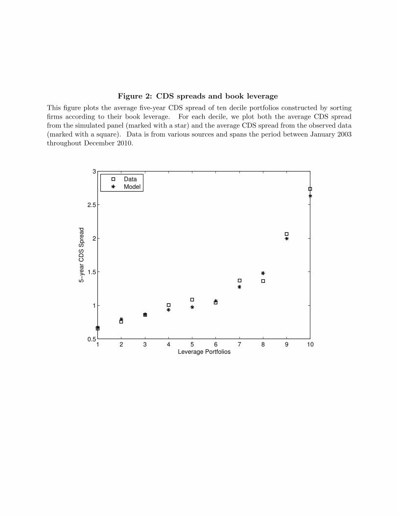
Figure 2: CDS spreads and book leverage

This figure plots the average five-year CDS spread of ten decile portfolios constructed by sortingfirms according to their book leverage. For each decile, we plot both the average CDS spreadfrom the simulated panel (marked with a star) and the average CDS spread from the observed data(marked with a square). Data is from various sources and spans the period between January 2003throughout December 2010.

1 2 3 4 5 6 7 8 9 100.5

1

1.5

2

2.5

3

Leverage Portfolios

5−

year

CD

S S

pre

ad

Data

Model

Figure 3: Book leverage portfolios

This figure plots the average book leverage of ten decile portfolios constructed by sorting firmsaccording to their book leverage. For each decile, we plot both the average leverage from theobserved data (marked with a square), the simulated panel from the base model (marked with astar) and the simulated panel from two versions of the model with fixed assets (marked with acircle and a pentagram). In the first version of the model, labeled Fixed Asset, we assign thesame initial capital to all firms in each simulated economy. In the second version of the model,labeled Fixed Asset Uniform, each firm is assigned an initial level of capital that is drowned fromthe uniform distribution across the the support of all possible levels of assets. In both cases, eachfirm is allowed to make investments equal to the annual depreciation so that, in effect, their capitalis fixed. Data is from various sources and spans the period between January 2003 throughoutDecember 2010.

1 2 3 4 5 6 7 8 9 100

0.2

0.4

0.6

0.8

1

1.2

1.4

1.6

Leverage Portfolios

Bo

ok L

eve

rag

e

Data

Base Model

Fixed Asset

Fixed Asset Uniform

Figure 4: Growth options and credit spread

At a given date we consider two firms with the same ratio of debt to asset in place (i.e., the samebook leverage). One of those two firms has just observed a positive realization of the idiosyncraticshock while the other has observed a negative realization. The first firm has growth options whilethe second does not. Because the shocks are persistent, the option to grow is due to the fact thatthe firm is on a high trajectory of the firm specific shock, and therefore expects also a positive shockin the next period. If that shock is large enough the firm will decide to invest. Therefore, sincewith one period debt the future investment, if there is one, is contextual to the repayment of the olddebt, high growth options are informative to bond-holders only because they convey informationabout future profitability. For this reason the relation between credit spread and growth optionsshould be negative, after controlling for book leverage.

t

(z, x)

t+ 1

(z′, x′)

firm chooses I ′

firm has a growth option if:k′ is small enoughz is large enough

firm repays b

and chooses b′firm repays b′

D/b′ is higher becausebondholders anticipate a large

cash flow at t+ 1

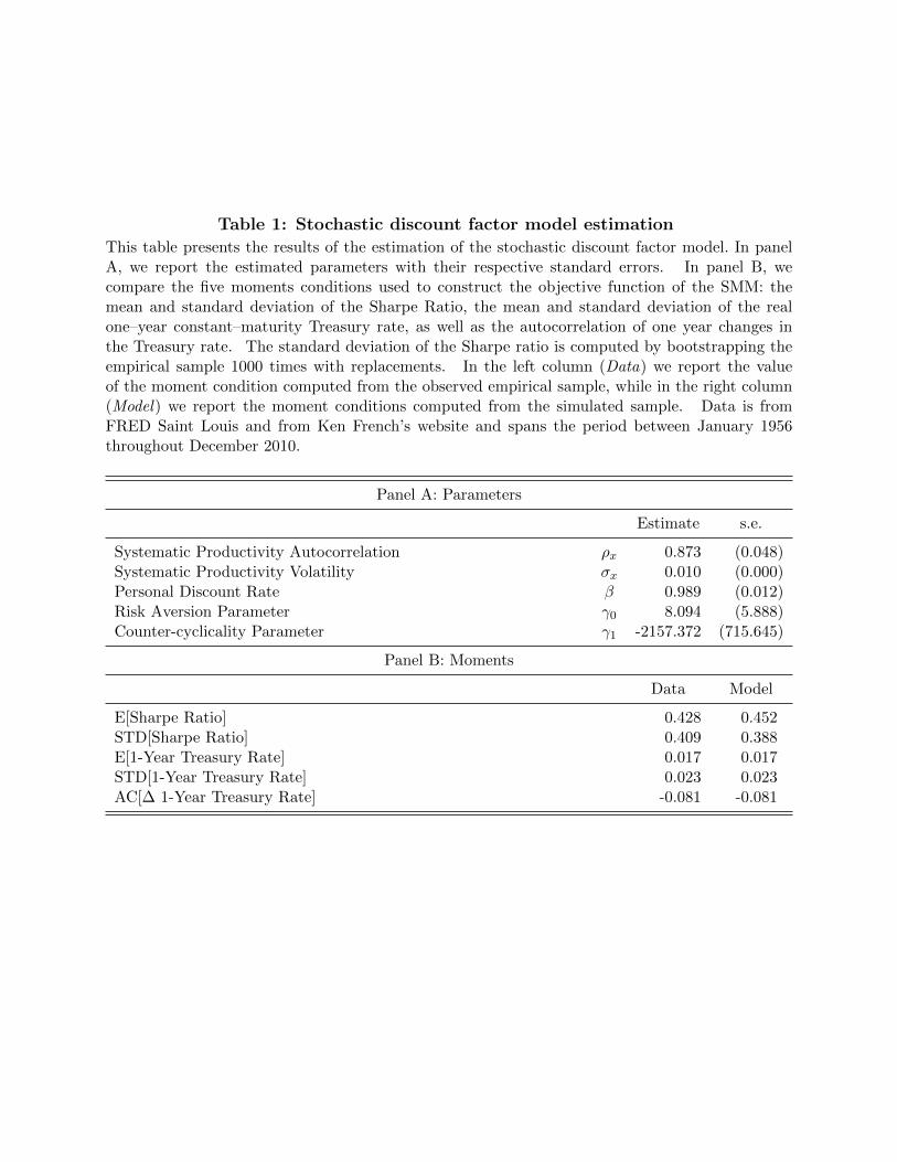
Table 1: Stochastic discount factor model estimation

This table presents the results of the estimation of the stochastic discount factor model. In panelA, we report the estimated parameters with their respective standard errors. In panel B, wecompare the five moments conditions used to construct the objective function of the SMM: themean and standard deviation of the Sharpe Ratio, the mean and standard deviation of the realone–year constant–maturity Treasury rate, as well as the autocorrelation of one year changes inthe Treasury rate. The standard deviation of the Sharpe ratio is computed by bootstrapping theempirical sample 1000 times with replacements. In the left column (Data) we report the valueof the moment condition computed from the observed empirical sample, while in the right column(Model) we report the moment conditions computed from the simulated sample. Data is fromFRED Saint Louis and from Ken French’s website and spans the period between January 1956throughout December 2010.

Panel A: Parameters

Estimate s.e.

Systematic Productivity Autocorrelation ρx 0.873 (0.048)Systematic Productivity Volatility σx 0.010 (0.000)Personal Discount Rate β 0.989 (0.012)Risk Aversion Parameter γ0 8.094 (5.888)Counter-cyclicality Parameter γ1 -2157.372 (715.645)

Panel B: Moments

Data Model

E[Sharpe Ratio] 0.428 0.452STD[Sharpe Ratio] 0.409 0.388E[1-Year Treasury Rate] 0.017 0.017STD[1-Year Treasury Rate] 0.023 0.023AC[∆ 1-Year Treasury Rate] -0.081 -0.081

Table 2: Firm model estimation

This table presents the estimation results of the firm model. In panel A, we report the 12 estimatedparameters with their respective standard errors. In panel B, we compare the 14 moments condi-tions used to construct the objective function of the SMM: the average book leverage, the averagefive-year CDS spread, the annual default frequency, the ratio of years in which the leverage sortingis valid over the total number of years, and the average five-year CDS spread of ten portfoliosconstructed by sorting firms into book leverage deciles. At the bottom of the table we reportthe 10 leverage portfolios mean absolute pricing error, the Hausman J-statistics and the respectivep-value in brackets. In the left column (Data) we report the value of the moment conditionscomputed from the observed empirical sample, while in the right column (Model) we report themoment conditions computed from the simulated sample. Data is from various sources and spansthe period between January 2003 throughout December 2010.

Panel A: Parameters

Estimate s.e.

Idiosyncratic Productivity Autocorrelation ρz 0.630 (0.292)Idiosyncratic Productivity Volatility σz 0.442 (0.199)Corporate Taxes τ 0.116 (0.224)Equity Issuance Cost ϕ 0.061 (0.101)Debt Adjustment Cost θ 0.086 (0.075)Production Function α 0.826 (0.140)Fix Cost f 0.609 (0.282)Distress Cost ξ 0.189 (0.098)Cost of Expansion λ1 0.002 (0.045)Cost of Contraction λ2 0.304 (0.157)Bankruptcy Cost η 0.499 (0.120)Recovery on Debt R 0.314 (0.126)

Panel B: Moments

Data Model

E[Book Leverage] 0.431 0.419E[5-year CDS Spread] 1.299 1.2931-year Default Frequency 0.491 0.521Valid Sortings 1.000 0.994

E[Leverage Portfolio CDS Spread]:1 Low Leverage 0.659 0.6702 0.760 0.7943 0.861 0.8664 1.007 0.9345 1.083 0.9756 1.042 1.0667 1.370 1.2768 1.360 1.4819 2.064 1.99610 High Leverage 2.738 2.631

Absolute Mean Pricing Error 0.064Hausman J-Statistic 4.103

[0.13]

Table 3: Dynamic Investment versus Fixed Asset

This table compares the estimation results of the base model (reported in Table 2) to estimationresults of two versions of the model that feature fixed asset as opposed to dynamic investment. Inthe first version of the model, labeled Fixed Asset, we assign the same initial capital to all firms ineach simulated economy. In the second version of the model, labeled Fixed Asset Uniform, eachfirm is assigned an initial level of capital that is drowned from the uniform distribution across thethe support of all possible levels of assets. In both cases, each firm is allowed to make investmentsequal to the annual depreciation so that, in effect, their capital is fixed. In Panel A we reportthe estimated parameters with t-statistics in parenthesis. In panel B, we compare the momentconditions used to construct the objective function of the SMM: the average book leverage, theaverage five-year CDS spread, the annual default frequency, the ratio of years in which the leveragesorting is valid over the total number of years. At the bottom of the table we report the 10leverage portfolios mean absolute pricing error, the Hausman J-statistics and the respective p-valuein brackets. Data is from various sources and spans the period between January 2003 throughoutDecember 2010.

Panel A: Parameters

Base Fixed FixedModel Asset Asset

Uniform

Idiosyncratic Productivity Autocorrelation ρz 0.630 0.884 0.601(0.29) (0.10) (0.03)

Idiosyncratic Productivity Volatility σz 0.442 0.399 0.144(0.20) (0.17) (0.02)

Corporate Taxes τ 0.116 0.109 0.244(0.22) (0.05) (0.08)

Equity Issuance Cost φ 0.061 0.031 0.069(0.10) (0.08) (0.09)

Debt Adjustment Cost θ 0.086 0.085 0.099(0.07) (0.12) (0.05)

Production Function α 0.826 0.790 0.836(0.14) (0.17) (0.12)

Fix Cost f 0.609 0.350 0.687(0.28) (0.16) (0.01)

Distress Cost ξ 0.189 0.003 0.009(0.10) (0.07) (0.05)

Cost of Expansion λ1 0.002(0.04)

Cost of Contraction λ2 0.304(0.16)

Bankruptcy Cost η 0.499 0.541 0.550(0.12) (0.17) (0.19)

Recovery on Debt R 0.314 0.201 0.232(0.13) (0.09) (0.11)

Panel B: Moments

Data Base Fixed FixedModel Asset Asset

Uniform

E[Book Leverage] 0.430 0.419 0.821 0.584E[5-year CDS Spread] 1.298 1.293 1.255 1.2471-year Default Frequency 0.491 0.521 0.491 0.622Valid sortings 1.000 0.994 0.073 0.977

E[Leverage Portfolio CDS Spread]:1 Low Leverage 0.657 0.670 0.061 0.0132 0.737 0.794 0.211 0.3163 0.885 0.866 0.430 0.6434 1.003 0.934 0.943 0.9625 1.077 0.975 0.773 1.2806 1.142 1.066 1.290 1.3697 1.336 1.276 1.617 1.5998 1.354 1.481 1.105 1.4499 2.036 1.996 1.616 1.68010 High Leverage 2.705 2.631 1.232 2.599

Absolute Mean Pricing Error 0.064 0.451 0.260Hausmann J-Statistic 4.103 1137.1 166.2

[0.13] [0.00] [0.00]

Table 4: Firm model estimation — 1 year CDS

This table presents the estimation results of the firm model. In panel A, we report the 12 estimatedparameters with their respective standard errors. In panel B, we compare the 14 moments condi-tions used to construct the objective function of the SMM: the average book leverage, the averageone-year CDS spread, the annual default frequency, the ratio of years in which the leverage sortingis valid over the total number of years, and the average one-year CDS spread of ten portfoliosconstructed by sorting firms into book leverage deciles. At the bottom of the table we reportthe 10 leverage portfolios mean absolute pricing error, the Hausman J-statistics and the respectivep-value in brackets. In the left column (Data) we report the value of the moment conditionscomputed from the observed empirical sample, while in the right column (Model) we report themoment conditions computed from the simulated sample. Data is from various sources and spansthe period between January 2003 throughout December 2010.

Panel A: Parameters

Estimate s.e.

Idiosyncratic Productivity Autocorrelation ρz 0.627 (0.091)Idiosyncratic Productivity Volatility σz 0.309 (0.072)Corporate Taxes τ 0.199 (0.106)Equity Issuance Cost φ 0.041 (0.131)Debt Adjustment Cost θ 0.000 (0.030)Production Function α 0.866 (0.019)Fix Cost f 0.619 (0.051)Distress Cost ξ 0.004 (0.108)Cost of Expansion λ1 0.017 (0.031)Cost of Contraction λ2 0.583 (0.176)Bankruptcy Cost η 0.547 (0.093)Recovery on Debt R 0.302 (0.324)

Panel B: Moments

Data Model

E[Book Leverage] 0.430 0.489E[1-year CDS Spread] 0.740 0.7571-year Default Frequency 0.491 0.515

E[Leverage Portfolio CDS Spread]:1 Low Leverage 0.360 0.3362 0.421 0.4493 0.551 0.5404 0.491 0.5625 0.640 0.6136 0.633 0.6687 0.862 0.7158 0.683 0.8519 1.278 1.00710 High Leverage 1.410 1.386

Absolute Mean Pricing Error 0.081Hausman J-Statistic 19.402

[0.00]

Table 5: Variants to the base-case model

This table presents the estimation results of variations of the firm model. In column (1) we reportthe parameters of the base model; in column (2) we report results of the model without financialdistress (No Diss); in column (3) we report the parameters of the model without fixed costs (NoFix); in column (4) we report the parameters of the model without adjustment costs to the capitalstock (No Adj); in column (5) we report the parameters of the model without equity issuancecost and debt adjustment costs (No Iss). In Panel A we report the estimated parameters witht-statistics in parenthesis. In panel B, we compare the moment conditions used to construct theobjective function of the SMM: the average book leverage, the average five-year CDS spread, theannual default frequency, the ratio of years in which the leverage sorting is valid over the totalnumber of years. At the bottom of the table we report the 10 leverage portfolios mean absolutepricing error, the Hausman J-statistics and the respective p-value in brackets. Data is from varioussources and spans the period between January 2003 throughout December 2010.

Panel A: Parameters

Base No Diss No Fix No Adj No Iss(1) (2) (3) (4) (5)

Idiosyncratic Productivity Autocorr. ρz 0.630 0.609 0.928 0.716 0.654(0.29) (0.07) (0.02) (0.05) (0.04)

Idiosyncratic Productivity Volatility σz 0.442 0.444 0.391 0.375 0.278(0.20) (0.07) (0.03) (0.04) (0.04)

Corporate Taxes τ 0.116 0.218 0.236 0.147 0.189(0.22) (0.08) (0.03) (0.04) (0.03)

Equity Issuance Cost ϕ 0.061 0.023 0.003 0.021(0.10) (0.05) (0.03) (0.06)

Debt Adjustment Cost θ 0.086 0.076 0.011 0.014(0.07) (0.02) (0.02) (0.02)

Production Function α 0.826 0.889 0.410 0.860 0.895(0.14) (0.04) (0.02) (0.02) (0.01)

Fix Cost f 0.609 0.559 0.533 0.651(0.28) (0.04) (0.04) (0.03)

Distress Cost ξ 0.189 0.275 0.070 0.027(0.10) (0.05) (0.04) (0.01)

Cost of Expansion λ1 0.002 0.228 0.002 0.014(0.04) (0.09) (0.02) (0.05)

Cost of Contraction λ2 0.304 0.494 0.755 0.439(0.16) (0.08) (0.05) (0.06)

Bankruptcy Cost η 0.499 0.463 0.543 0.527 0.521(0.12) (0.07) (0.04) (0.11) (0.03)

Recovery on Debt R 0.314 0.311 0.315 0.301 0.335(0.13) (0.05) (0.05) (0.06) (0.11)

Panel B: Moments

Data Base No Diss No Fix No Adj No Iss

E[Book Leverage] 0.430 0.419 0.467 0.635 0.474 0.440E[5-year CDS Spread] 1.298 1.293 1.278 0.362 1.326 1.2691-year Default Frequency 0.491 0.521 0.518 0.126 0.562 0.542Valid sortings 1.000 0.994 0.947 0.074 0.961 0.969

E[Leverage Port. CDS Spread]:1 Low Leverage 0.657 0.670 0.579 0.596 0.645 0.6372 0.737 0.794 0.765 0.313 0.801 0.8053 0.885 0.866 0.885 0.858 0.871 0.9064 1.003 0.934 0.972 1.015 0.963 0.9485 1.077 0.975 1.047 0.935 1.067 1.0246 1.142 1.066 1.145 1.286 1.225 1.0977 1.336 1.276 1.257 1.208 1.343 1.3038 1.354 1.481 1.445 1.371 1.546 1.4609 2.036 1.996 1.845 1.713 1.895 1.79010 High Leverage 2.705 2.631 2.405 1.940 2.480 2.414

Absolute Mean Pricing Error 0.064 0.083 0.204 0.079 0.094Hausman J-Statistic 4.103 26.826 2193.8 18.738 7.042

[0.13] [0.00] [0.00] [0.00] [0.13]

Table 6: Subsamples

This table presents the estimation results of the firm model in two separate sub-samples: 2003-2006 and 2007-2010 respectively. In panel A, we report the 12 estimated parameters with theirrespective standard errors. In panel B, we compare the 14 moments conditions used to constructthe objective function of the SMM: the average book leverage, the average five-year CDS spread,the annual default frequency, the ratio of years in which the leverage sorting is valid over the totalnumber of years, and the average five-year CDS spread of ten portfolios constructed by sorting firmsinto book leverage deciles. At the bottom of the table we report the 10 leverage portfolios meanabsolute pricing error, the Hausman J-statistics and the respective p-value in brackets. In thecolumns labeled Data we report the value of the moment conditions computed from the observedempirical sample, while in the columns labeled Model we report the moment conditions computedfrom the simulated sample. Data is from various sources and spans the period between January2003 throughout December 2010.

Panel A: Parameters

2003-2006 2007-2010

Idiosyncratic Productivity Autocorrelation ρz 0.741 0.601(0.08) (0.14)

Idiosyncratic Productivity Volatility σz 0.245 0.441(0.03) (0.10)

Corporate Taxes τ 0.159 0.111(0.06) (0.14)

Equity Issuance Cost φ 0.029 0.051(0.09) (0.08)

Debt Adjustment Cost θ 0.024 0.099(0.06) (0.07)

Production Function α 0.882 0.847(0.21) (0.11)

Fix Cost f 0.565 0.648(0.12) (0.03)

Distress Cost ξ 0.005 0.072(0.14) (0.15)

Cost of Expansion λ1 0.165 0.011(0.07) (0.06)

Cost of Contraction λ2 0.512 0.522(0.27) (0.15)

Bankruptcy Cost η 0.546 0.549(0.11) (0.18)

Recovery on Debt R 0.454 0.210(0.22) (0.32)

Panel B: Moments

2003-2006 2007-2010Data Model Data Model

E[Book Leverage] 0.422 0.460 0.431 0.440E[5-year CDS Spread] 0.711 0.681 1.886 1.8061-year Default Frequency 0.266 0.286 0.715 0.932Valid sortings 1.000 0.980 1.000 0.986

E[Leverage Portfolio CDS Spread]:1 Low Leverage 0.446 0.308 0.867 0.8722 0.367 0.378 1.107 1.1323 0.478 0.442 1.291 1.3304 0.509 0.514 1.497 1.5175 0.584 0.559 1.569 1.5646 0.571 0.631 1.712 1.6517 0.756 0.709 1.916 1.8868 0.815 0.831 1.892 2.1669 1.075 0.966 2.997 2.55410 High Leverage 1.414 1.312 3.996 3.152

Pricing error 0.055 0.174J-stat 3.127 4.737

[0.22] [0.09]

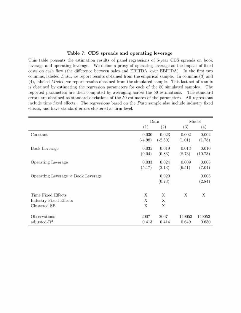
Table 7: CDS spreads and operating leverage

This table presents the estimation results of panel regressions of 5-year CDS spreads on bookleverage and operating leverage. We define a proxy of operating leverage as the impact of fixedcosts on cash flow (the difference between sales and EBITDA, over EBITDA). In the first twocolumns, labeled Data, we report results obtained from the empirical sample. In columns (3) and(4), labeled Model, we report results obtained from the simulated sample. This last set of resultsis obtained by estimating the regression parameters for each of the 50 simulated samples. Thereported parameters are then computed by averaging across the 50 estimations. The standarderrors are obtained as standard deviations of the 50 estimates of the parameters. All regressionsinclude time fixed effects. The regressions based on the Data sample also include industry fixedeffects, and have standard errors clustered at firm level.

Data Model(1) (2) (3) (4)

Constant -0.030 -0.023 0.002 0.002(-4.98) (-2.50) (1.01) (1.78)

Book Leverage 0.035 0.019 0.013 0.010(9.04) (0.83) (8.73) (10.73)

Operating Leverage 0.033 0.024 0.009 0.008(5.17) (2.13) (6.51) (7.04)

Operating Leverage × Book Leverage 0.020 0.003(0.73) (2.84)

Time Fixed Effects X X X XIndustry Fixed Effects X XClustered SE X X

Observations 2007 2007 149053 149053adjusted-R2 0.413 0.414 0.649 0.650

Table 8: CDS portfolio sorting by book leverage and operating leverage

This table reports independent quartile portfolio sorting of CDS spreads by book leverage andoperating leverage. In Panel A we report results obtained from the empirically observed data(Data), while in Panel B we report results for the simulated sample (Model). The sorting procedurein the case of the simulated sample involves first sorting in each time period of each one of the 50simulated samples. Next, we average across time. Finally, the results reported are obtained byaveraging across the 50 simulated samples.

Panel A: Data

Operating LeverageLow (2) (3) High H – L t-stat

Low Book Leverage 0.540 0.645 0.763 1.012 0.472 (3.61)(2) 0.746 0.650 0.866 1.770 1.024 (4.12)(3) 0.880 0.996 1.054 1.953 1.073 (3.77)High Book Leverage 1.850 1.586 1.820 3.398 1.548 (3.55)

Panel B: Model

Operating LeverageLow (2) (3) High H – L t-stat

Low Book Leverage 0.628 0.694 0.767 1.059 0.424 (4.72)(2) 0.757 0.777 0.965 1.615 0.858 (6.29)(3) 0.881 0.891 1.137 1.912 1.038 (6.54)High Book Leverage 1.576 1.369 2.024 2.467 1.361 (6.24)

Table 9: CDS spreads and market–to–book ratio

This table presents the estimation results of panel regressions of 5-year CDS spreads on bookleverage and market–to–book ratio, Q. In the first two columns, labeled Data, we report resultsobtained from the empirical sample. In columns (3) and (4), labeled Model, we report resultsobtained from the simulated sample. This last set of results is obtained by estimating the regressionparameters for each of the 50 simulated samples. The reported parameters are then computed byaveraging across the 50 estimations. The standard errors are obtained as standard deviations ofthe 50 estimates of the parameters. All regressions include time fixed effects. The regressionsbased on the Data sample also include industry fixed effects, and have standard errors clustered atfirm level.

Data Model(1) (2) (3) (4)

Constant 0.016 -0.030 0.018 0.013(4.33) (-4.86) (9.32) (11.76)

Book Leverage 0.034 0.102 0.031 0.033(8.94) (10.46) (11.35) (10.93)

Q -0.009 0.007 -0.005 -0.004(-8.62) (4.02) (-6.92) (-8.37)

Q × Book Leverage -0.046 -0.001(-8.79) (-4.18)

Time Fixed Effects X X X XIndustry Fixed Effects X XClustered SE X X

Observations 2007 2007 149053 149053Adjusted-R2 0.444 0.505 0.755 0.761

Table 10: CDS portfolio sorting by book leverage and market–to–book ratio

This table reports independent quartile portfolio sorting of CDS spreads by book leverage andmarket–to–book. In Panel A we report results obtained from the empirically observed data (Data),while in Panel B we report results for the simulated sample (Model). The sorting procedure inthe case of the simulated sample involves first sorting in each time period of each one of the 50simulated samples. Next, we average across time. Finally, the results reported are obtained byaveraging across the 50 simulated samples.

Panel A: Data

Market to Book RatioLow (2) (3) High H – L t-stat

Low Book Leverage 1.215 0.788 0.691 0.510 -0.706 (-2.06)(2) 1.635 1.026 0.739 0.519 -1.116 (-2.93)(3) 1.766 1.234 0.959 0.652 -1.114 (-2.75)High Book Leverage 4.068 2.450 1.404 0.668 -3.400 (-3.46)

Panel B: Model

Market to Book RatioLow (2) (3) High H – L t-stat

Low Book Leverage 0.901 0.679 0.586 0.505 -0.399 (-5.44)(2) 1.551 0.913 0.707 0.603 -1.074 (-6.90)(3) 2.201 1.279 0.925 0.748 -1.453 (-8.38)High Book Leverage 2.964 2.288 1.905 1.807 -1.112 (-7.47)

Table

11:

CD

Sand

mark

et–

to–b

ook

—se

nsi

tivit

yanaly

sis

Th

ista

ble

pre

sents

regr

essi

ons

ofC

DS

spre

ads

onle

ver

age

and

mar

ket–

to–b

ook

rati

osin

sim

ula

ted

sam

ple

s.E

ach

regre

ssio

nh

as

the

sam

esp

ecifi

cati

onas

colu

mn

3of

Tab

le9.

Eac

hsi

mu

late

dsa

mp

leis

obta

ined

by

sim

ula

tin

gth

em

od

elke

epin

gth

ese

tof

esti

mate

dp

aram

eter

sre

por

ted

inT

able

2,b

ut

per

turb

ing

the

auto

corr

elat

ion

ofth

eid

iosy

ncr

atic

shock

(ρz)

and

the

pro

du

ctio

nfu

nct

ion

para

met

er(α

)in

the

inte

rval

[−0.0

5,0.

05]

arou

nd

the

resp

ecti

veva

lues

rep

orte

din

Tab

le2,ρz

=0.

630

andα

=0.

826.

Bec

au

sech

an

gin

gth

eop

tim

al

par

amet

ers

pro

du

ces

mor

esk

ewed

sam

ple

s,w

est

and

ard

ize

all

vari

able

sb

efor

ees

tim

atio

n.

Eac

hre

port

edco

effici

ent

rep

rese

nts

the

cred

itsp

read

chan

ge,

exp

ress

edin

por

tion

ofa

stan

dar

dd

evia

tion

,th

atco

rres

pon

ds

toa

one

stan

dar

dd

evia

tion

chan

ge

inth

ele

fth

an

dsi

de

vari

able

.W

eal

sore

por

ta

coeffi

cien

tt-

stat

isti

csas

wel

las

the

t-st

atis

tic

ofa

test

onth

ediff

eren

ceb

etw

een

the

esti

mate

dre

gre

ssio

nco

effici

ents

onQ

obta

ined

from

the

orig

inal

sam

ple

and

thos

eob

tain

edfr

omth

ep

ertu

rbed

sam

ple

s.

Idio

syn

crat

icsh

ock

auto

corr

elat

ion

par

amet

erρz−

0.05

ρz−

0.0

2ρz−

0.01

ρz

ρz

+0.0

1ρz

+0.0

2ρz

+0.0

5

Book

Lev

erag

e1.

281

1.35

31.

366

1.39

11.4

43

1.4

60

1.4

22

(77.

50)

(72.

11)

(70.

71)

(66.

49)

(64.1

8)

(61.6

0)

(59.8

4)

Q-0

.666

-0.7

74-0

.778

-0.8

42-0

.849

-0.8

85

-0.8

95

(-75

.45)

(-70

.06)

(-65

.76)

(-71

.09)

(-56.0

9)

(-57.0

4)

(-69.2

3)

t-st

atd

iffer

ence

inQ

par

amet

er(-

50.4

8)(-

21.0

5)(-

23.7

1)(2

.01)

(10.4

4)

(13.7

6)

std

(CD

S)

0.00

70.

007

0.00

70.

007

0.0

07

0.0

07

0.0

07

std

(Book

Lev

erag

e)0.

335

0.35

20.

390

0.39

40.4

36

0.4

44

0.4

69

std

(Q)

1.26

51.

490

1.63

81.

773

1.8

57

2.0

05

2.4

74

Pro

du

ctio

nfu

nct

ion

par

amet

erα−

0.0

5α−

0.02

α−

0.0

1α

α+

0.0

1α

+0.0

2α

+0.0

5

Book

Lev

erag

e1.

344

1.38

41.

403

1.35

21.3

38

1.3

03

1.2

31

(74.

99)

(72.

28)

(66.

41)

(71.

72)

(74.4

6)

(88.3

0)

(79.4

2)

Q-0

.824

-0.8

14-0

.813

-0.7

87-0

.706

-0.6

48

-0.5

18

(-74

.70)

(-64

.22)

(-57

.06)

(-76

.02)

(-67.5

3)

(-82.5

7)

(-88.7

1)

t-st

atd

iffer

ence

inp

aram

eter

(9.7

2)(6

.43)

(7.0

3)(-

26.5

6)

(-46.5

7)

(-60.4

4)

std

(CD

S)

0.00

70.

007

0.00

70.

007

0.0

07

0.0

07

0.0

07

std

(Book

Lev

erag

e)0.

404

0.40

70.

410

0.37

20.3

90

0.3

61

0.3

42

std

(Q)

1.80

61.

725

1.71

31.

672

1.6

03

1.5

73

1.4

43

Table 12: CDS spreads and growth opportunities

This table presents the estimation results of panel regressions of 5-year CDS spreads on bookleverage, present value of asset in place (PV AP ), present value of growth opportunities (PV GO),and market–to–book ratio. All results are obtained by estimating the regression parameters foreach of the 50 simulated samples and subsequently averaging across the 50 estimations. Thestandard errors are obtained as standard deviations of the 50 estimates of the parameters. Allregressions include time fixed effects.

(1) (2) (3) (4) (5)

Constant 0.020 0.006 0.016 0.018 0.026(9.09) (7.06) (7.82) (9.20) (8.78)

Leverage 0.016 0.038 0.034 0.030(9.05) (12.75) (13.40) (11.51)

PVAP -0.006 -0.004 -0.011(-6.80) (-5.61) (-5.69)

PVGO -0.007 -0.006 -0.001(-7.22) (-7.92) (-2.16)

Q -0.005 0.004(-6.81) (4.12)

Time Fixed Effects X X X X X

Observations 149053 149053 149053 149053 149053Adjusted-R2 0.678 0.725 0.768 0.755 0.538

Table 13: CDS spreads and lagged asset and debt values

This table presents the estimation results of panel regressions of 5-year CDS spreads on current andlagged values of asset and debt. In the first three columns, labeled Data, we report results obtainedfrom the empirical sample. In columns (4) to (6), labeled Model, we report results obtained fromthe simulated sample. This last set of results is obtained by estimating the regression parametersfor each of the 50 simulated samples. The reported parameters are then computed by averagingacross the 50 estimations. The standard errors are obtained as standard deviations of the 50estimates of the parameters. All regressions include time fixed effects. The regressions basedon the Data sample also include industry fixed effects, and have standard errors clustered at firmlevel.

Data Model(1) (2) (3) (4) (5) (6)

Constant 0.017 0.075 0.073 0.017 0.024 0.023(4.65) (9.23) (8.98) (8.21) (5.97) (5.95)

Book Leverage 0.038 0.030(8.76) (11.02)

Q -0.010 -0.010 -0.009 -0.005 -0.002 -0.002(-8.43) (-8.67) (-7.55) (-6.42) (-2.81) (-2.76)

Current Asset -0.011 -0.020 -0.005 -0.007(-8.16) (-5.39) (-5.89) (-6.97)

Current Debt 0.007 0.007 0.009 0.014(5.85) (4.43) (8.68) (8.50)

Lag Asset 0.009 0.003(2.59) (9.88)

Lag Debt -0.000 -0.005(-0.19) (-7.38)

Time Fixed Effects X X X X X XIndustry Fixed Effects X X XClustered SE X X X

Observations 1822 1822 1566 134107 134107 133495Adjusted-R2 0.429 0.405 0.451 0.756 0.480 0.497

Table 14: Changes in CDS spreads and changes in leverage

This table presents the estimation results of panel regressions of changes in 5-year CDS spreadson changes in debt and changes in asset. In the first two columns, labeled Data, we reportresults obtained from the empirical sample. In columns (3) to (4), labeled Model, we reportresults obtained from the simulated sample. This last set of results is obtained by estimating theregression parameters for each of the 50 simulated samples. The reported parameters are thencomputed by averaging across the 50 estimations. The standard errors are obtained as standarddeviations of the 50 estimates of the parameters. All regressions include time fixed effects. Theregressions based on the Data sample also include industry fixed effects, and have standard errorsclustered at firm level.

Data Model(1) (2) (3) (4)

Constant -0.001 -0.002 -0.001 -0.001(-0.45) (-1.42) (-0.68) (-0.73)

Change in Book Leverage 0.023 0.019(2.83) (8.72)

Profitability -0.004 -0.001 -0.000 -0.001(-0.93) (-0.17) (-1.28) (-3.10)

Change in Debt 0.005 -0.002(2.98) (-4.82)

Investment -0.004 -0.003(-2.33) (-9.53)

Disinvestment 0.031 0.056(2.95) (13.82)

Time Fixed Effects X X X XIndustry Fixed Effects X XClustered SE X X

Observations 1184 1184 131386 131386Adjusted-R2 0.363 0.365 0.347 0.350