First Cut is the Deepest: On Optimal AcceptanceStrategies in Real Estate

Thomas Emmerling, Abdullah Yavas and Yildiray Yildirim ∗

Current version: August 25, 2013

Abstract

We consider the problem of a seller who faces an unknown number of offers whereeach offer is a random draw from a known distribution. The objective of the seller is tomaximize the probability that the highest offer is chosen. This is equivalent to maximizingexpected utility when one assigns preferences to rankings of offers. We identify the optimalselling strategy using the technique of Porosinski (1987) and general optimal stoppingtheory. We show that the optimal strategy is characterized by a non-increasing stochasticset of reservation prices. This is in contrast to the classical search theory models wherereservation prices are deterministic. Our analysis also provides theoretical support to theobservation that first offers in residential real estate markets should be accepted moreoften since they tend to be higher than subsequent offers.

1 Introduction

Consider the problem of a home seller who expects to receive an unknown number of offers

on her house. When an offer arrives, the seller must either accept it, in which case the search

process stops, or reject it and wait for a new offer. If the seller rejects the offer, another offer may

or may not arrive, and if a new offer arrives it might be higher or smaller than the current offer.

Furthermore, the seller is not able to go back and choose a previously rejected offer. Deciding

whether or not it is optimal to accept an offer in such an environment is a complicated task.

The standard approach in the literature has been to utilize the optimal stopping rule where the

∗Emmerling, tjemmerl@syr.edu, Whitman School of Management, Syracuse University, 721 University AveSuite 120, Syracuse, NY 13244; Yavas, ayavas@bus.wisc.edu, Wisconsin School of Business, Grainger Hall,975 University Avenue, Madison, WI, 53706; Yildirim, yildiray@syr.edu, Whitman School of Management,Syracuse University, 721 University Ave Suite 500, Syracuse, NY 13244. We thank Robert Jarrow, participantsof the April 2013 AMS Eastern Section Special Session on Financial Mathematics in Boston, MA and those inattendance for the Finance Department Seminar of the Whitman School of Management at Syracuse Universityfor valuable comments and suggestions.

seller incurs a search cost to obtain a new offer and rejects the offer if the value of continued

search exceeds the cost of search. However, most home sellers hire a broker to help them sell

their property. The broker typically incurs the search costs and conducts the search process on

behalf of the seller. If there is a successful transaction, the seller owes the broker a percentage

of the transaction price as commission. Since the commission is not a function of the number

of buyers contacted or the number of bids received, the seller is often not concerned with the

cost of obtaining another bid. In fact, the seller would rather have as many buyers contacted

and as many bids obtained as possible.

In this paper, we recognize this important aspect of the home selling process and model

the seller’s objective as maximizing the probability of accepting the highest bid. That is, the

seller’s problem is to maximize the probability that the offer she chooses is higher than the

offers she has rejected and higher than the offers she might have received if she continued the

search process. This objective is equivalent to maximizing expected utility when one assigns

preferences to rankings of offers. More specifically, the owner of the property receives Ui units

of utility if the accepted item is the i-th best of all that are offered; additionally, the units

of utility Ui are non increasing in the ranking i. Our analysis focuses upon the special case

U1 = 1, Uj = 0, j ≥ 2 with a goal of maximizing the seller’s expected utility. This corresponds to

a seller’s objective of following a strategy which accepts the highest offer (relative to all others)

with the greatest probability. Evidence from real estate markets indicates that sellers adjust

listing prices so as to maximize sale prices. Prior to further adjustments enacted to induce

offer frequency and/or distribution changes, sellers wish to pick the largest offer presented to

them. Following such a strategy, sellers are interested in how a current offer compares to both

previous and future offers. In this way, past offers can act as a reference point for judging the

attractiveness of a current offer which is reminiscent of modified expected utility theory.

The alternative preference structure and objective we analyze provides an optimal strat-

egy which closely resembles observed seller behavior of “past offer regret” within behavioral

economic theory. This suggests that our setup might be able to be embedded within modified

expected utility theory such as prospect theory. In Appendix A, we analyze this conjecture using

a simple model within our framework and show that our perspective embraces the observable

behavioral tendencies of prospect theory and yet is outside its purview.

Our model captures another important feature of the search process by making the number

2

of bids received stochastic. The seller has to decide whether to accept or reject an offer without

knowing whether another offer would arrive. This is a departure from standard search models

in the real estate literature where the seller can obtain another bid by incurring a search cost.

Modifying the standard approach to capture this realistic aspect of the seller’s problem makes

the current analysis much more complicated than the standard search models. In this paper,

we take up this challenge and derive the optimal strategy for a seller who faces an uncertain

number of buyers as well as a random bid that a buyer may offer.

In this more complicated set up, we are still able to solve for a simple optimal strategy for

the seller. A distinguishing feature of our optimal strategy is its stochastic nature. In classical

search theory, the optimal strategy is characterized by a deterministic non-increasing (in bids)

set of reservation prices which dictate levels at or above which a bid is acceptable. Within

our framework, we find that acceptable bids cannot simply be characterized as those above a

certain deterministic number. Rather, bids also need to be examined in relation to each other

when determining if a given bid should be accepted. To be more precise, the optimal decision

to accept a bid requires not only that the bid exceeds a certain threshold level, but it also

needs to be greater than all past (random) bids received. In addition, we are able to calculate

the probability of accepting the highest offer (among offers received and were to be received

if current offer rejected), estimate a confidence interval for this probability and show how it

changes as the seller rejects an offer and waits for the arrival of a new offer. We also show that

if an improvement in market conditions leads to a rise in the expected number of bids, this can

lead to a decrease as well as an increase in the probability of a sale.

The likelihood of future bids in real estate markets depends upon many factors such as

the availability of financing, prevailing interest rates, income per capita, unemployment rate,

supply of new units, property taxes etc. In our analysis, we are able to incorporate the impact

of such uncertain factors and examine their impact on the seller’s optimal strategy. Within

our framework, we also specifically incorporate anecdotal evidence that first bids on real estate

property tend to be larger than subsequent bids. A possible explanation for such a phenomenon

might be that a newly listed property attracts the attention of all the buyers in the market

whereas a property that has been listed for some time only attracts the attention of new buyers

entering the market. Another possible reason might be the signal that prospective home buyers

may infer about the quality of the property from the amount of time it spends on the market,

3

according to which the interest in the property will decline as the property stays longer (Taylor

(1999)). In contrast to the classical search model literature, we provide a solution for the

optimal selling strategy which does not rule out the presence of distributionally different first

bids from all subsequent bids. In fact, for an objective of maximizing the probability that

the seller accepts the largest of all bids offered, the optimal strategy in this non independent

and identically distributed case (non-idd) is precisely the same as the strategy for the classical

(iid) case, i.e., the reservation prices are identical in both cases. A direct consequence of this

fact is that first bids will be optimally accepted with greater likelihood if they are in fact

distributionally superior (e.g., the median of the first bid distribution exceeds the median of

subsequent bids) rather than identical. The empirical findings of Merlo and Ortalo-Magne

(2004) that more than seventy percent of the properties sell to the first potential buyer making

an offer on the property supports this prediction of our model.

The paper proceeds as follows: Section 2 provides motivation of our model as a variation

of the classical secretary problem. Section 3 discusses the model and optimal strategy for our

selling problem. Section 4 presents numerical results pertaining to the Gamma distribution for

bid sizes and the Poisson distribution for the number of bids. Here, we approximate threshold

strategies associated to the optimal selling policy and discuss distributional properties of the

optimal policy. Section 5 concludes the paper. Finally, we include an appendix containing

some technical aspects regarding the optimal policy along with numerical results when the

distribution of the bid size is either uniform or one-point distributed.

2 Background

The problem of deciding when to accept a given offer for an asset can be viewed as a variation

of what is known as the secretary problem in probability theory (see Freeman (1983)). The

standard secretary problem can be stated as follows: A fixed number of items n are to be

presented to an observer one by one in random order with all n! possible orders being equally

likely. Each item is comparable to any other and as each item is presented, the observer must

decide whether to accept it or not. If the observer accepts an item, then the process stops. If the

observer rejects the item, then the next item in the sequence is presented and the observer faces

the same choice as before. If the last item is presented, it must be accepted. The observer’s

4

aim is to find an optimal acceptance policy.

The seller of real estate faces a similar problem to this classically motivated problem. Over

time, perspective buyers present offers in sequence to purchase the property and the seller

must decide if it is acceptable or not. If the seller feels that the offer is too low (based upon

valuations, perspective future offers etc), they will reject the bid in favor of waiting for a better

offer. However, if the offer meets an appropriately determined threshold level (reservation price),

then the offer will be accepted and the property will be sold. A simple model for this problem

corresponds to the seller drawing from n independently distributed random offers in sequence

and deciding after each draw whether or not to accept the offer. When bids are observed

sequentially from a known distribution, the problem is said to have “full information”. Early

work on optimal behavior in this full information setting was carried out by Guttman (1960).

Guttman (1960) found the stopping rule yielding the largest expected payoff when there are at

most n (fixed, known) choices. Further, each independent selection was drawn from a common,

general distribution function. This analysis by Guttman (1960) served as a direct extension of

a similar analysis carried out for the uniform distribution by Moser (1956). Similar to both

Guttman (1960) and Moser (1956), our analysis to follow also seeks an optimal stopping time

except with a modified objective. In our analysis, we seek a stopping time which maximizes

the probability of accepting the largest bid. Our setting is more general than Guttman (1960)

in that we allow for a random number of bids and consider the possibility that all bids are not

identically distributed.

In our analysis to follow, we will operate exclusively within the “full information” setting

and analyze our real estate problem with a random number of bids. In order to capture both

the notion that “first offers tend to be larger than later bids” and the uncertain number of

bids a property may receive, we will suppose that the distributions of the first bid can be

different from all other bids and the number of bids is random. This setting and objective most

closely resembles the optimal stopping problem solved in Porosinski (1987). The important

difference between Porosinski (1987) and our present work is that we do not assume all bids

to be identically distributed. In what follows, we will show that calculating the optimal selling

strategy in this context is no different than in the iid setting of Porosinski (1987).

As we have mentioned, differences in bid distributions is a key feature of our model. Such

heterogeneity of bid distributions within the model presents interesting research questions re-

5

lated to estimation of bid distributions. Although this is not our focus in the present analysis,

it is worth mentioning two papers related to the estimation of bid distributions within classical

models: Tryfos (1981) and Brown and Brown (1986). Firstly, Tryfos (1981) develops a proce-

dure by which the distribution of bids may be estimated on the basis of a sample of real estate

transactions recording the asking price, the selling price and the physical characteristics of the

properties sold. Secondly, Brown and Brown (1986) develop a methodology based on order

statistics for estimating the parameters of the bid distribution which has not yet been placed

on the market.

3 Model Setup and Solution

Up through the present, the most common approach for solving the real estate selling problem

has been to utilize the job search theory. This literature was initiated by Stigler (1961) and

was subsequently developed and discussed by many including Lippman and McCall (1976),

Lancaster and Chesher (1983), van den Berg (1990) etc. Overall, the job search theory applies

optimal stopping theory to investigate how many searches an unemployed person should un-

dertake before accepting a job when search has a cost; e.g., time, lost wages. Applying this

theory to the real estate selling problem, we have the following model: Suppose offers arrive for

a real estate asset where Xn denotes the amount of the offer received at time n. For simplicity,

assume offers arrive independently and all have the same distribution which is known to the

seller. Further, search incurs a unit cost c > 0. When the seller receives an offer, she must

decide whether to accept it or wait for a better offer. The criteria for deciding whether or not

to accept an offer is determined by finding the strategy which maximizes the expected payoff

from the sale of the asset over all possible random selling times, i.e.,

supτ∈T

E[Yτ ], where

Yn = Xn − nc, n = 1, 2, . . . .

(JS)

6

An investigation into this optimal stopping problem yields an explicit optimal strategy (i.e., a

strategy which attains the optimal expected value above) of the form,

τ ∗ := min n ≥ 1 : Xn ≥ r(n),

for some calculated value r(n). In the literature, r(n) is known as the reservation price at time

n since it denotes the smallest offer that will be accepted. The optimal strategy is to accept an

offer for period n if the offer is greater than or equal to the reservation price for period n.

Our analysis to follow seeks to depart from the usual job search methodology in several

important ways. First, there is anecdotal evidence that the first offer for a real estate asset

tends to be the highest. This observation suggests that the distribution of the first offer X1 is

fundamentally different from all other offers. This lies in contrast to the classical job search

iid assumption for bids Xn, n = 1, 2, . . .. Next, it is more realistic to believe that the number

of bids that arrive for the real estate asset is not known beforehand as opposed to the usual

assumptions of a known fixed number such as N = 1, 2, . . . ,∞. For example, the number of

bids N often depends upon many factors such as: the time of year, the quality of the asset,

the state of the overall economy, the time on the market etc and is not simply available upon

payment of cost c > 0 for each additional bid. Finally, given the anecdotal evidence that first

offers tend to be largest and a clear desire of a seller to develop a strategy to exploit this, we

decide to shift the objective of the seller away from the optimal strategy which maximizes, on

average, the net payoff Yτ∗ = Xτ∗ − τ ∗c in favor of one which maximizes the probability that

the highest offer is chosen. Thus, we replace the usual objective function (JS) of the job search

model with one that emphasizes the importance of choosing the largest bid made to the seller.

As indicated earlier, this objective function for the seller is particularly more appropriate for

sellers in real estate markets who often hire a real estate broker to carry out the search process

and incur the search costs of contacting potential buyers. The primary search cost for the seller

is the brokerage commission that she has to pay, and this commission is independent of the

number of offers received and does not change depending on whether or not an offer is accepted

(whether the brokerage fee is incurred is, of course, contingent on a sale)1.

1Note that search cost c does not affect the optimal strategy of the seller when the objective is to maximizethe probability of accepting the highest bid. One could modify the objective to analyze the probability ofobtaining the highest bid net of costs. This could be examined in future work but would not be appropriate for

7

Our analysis below operates in discrete time, i.e., t = 1, 2, . . .. At each point in time, the

seller knows whether or not there is an offer and can decide to accept it or not. If the seller

turns down an offer, she cannot recall it later and it may be the last offer presented for the

property. The seller learns whether or not a particular offer was the last one to be offered

exactly one time unit after she rejected the offer. The goal for the seller is to identify a criteria

for accepting a particular offer as the selling problem evolves. Given this brief description, we

now mathematically ground this model. We assume the following conditions hold.

Assumption 1. (1) the offer bids X1 ∼ F1, Xi ∼ F, i ≥ 1 make up a sequence of indepen-

dent random variables with continuous cumulative distribution functions defined on the

probability space (Ω,F ,P); where Ω is the probability sample space, P is the probability

measure on Ω, and F is the collection of sets (σ-algebra) for which we can determine the

P-probability. Further, we assume that the support of the bid distributions are identical

for all bids. Finally, all bids is bounded from below by R > 0, i.e, Xi > R with probability

one for all i ≥ 1.

(2) the number of observations N is a random variable independent of the sequence (Xi)ni=1

with a known distribution,

P(N = n) = pn, n = 0, 1, 2, . . . ,∞∑n=0

pn = 1.

Assumption 1 captures the notion that the first bid is distributionally different from subse-

quent bids. The additional assumption that the support of each distribution is bounded from

below by R is not required for solving the objective problem stated below. We add this addi-

tional requirement in order incorporate the realistic notion of a minimally acceptable sale price.

Namely, we assume that the seller has a price R > 0 such that they will not go below when

selling the real estate. That is, R represents the price below which the seller prefers holding

the property than selling it. Hence R captures the utility that the seller will derive from the

property if the property does not get sold. Given this, offers which are below R will not even

be considered qualified bids for the sale of the real estate. For this reason, we assume bids are

bounded from below by R. Additionally, Assumption 1 allows us to consider the situation in

sellers who hire brokers and simply pay a commission upon sale.

8

which the number of bids N is a random variable with a known distribution. Notice that since

N is random, the seller faces an additional risk; if they reject any bid, they may then discover

that it was the last one, in which case the opportunity to sell the property is lost.

Notice that in Assumption 1, we still retain independence between bids. While leaving an

analysis of the non-independent case to future research, here we incorporate our motivating

observation between first bids and all others to follow through our distributional assumption

on the bids. We take the point of view that bidders do not have information about previous

bid amounts when making an offer. 2 Rather, the reality that a particular bid is not the first

bid means that it comes from a different prescribed distribution.

The goal of our analysis is to identify a criteria (or rule) used to evaluate whether a currently

presented bid should be accepted or not. An example of such a rule might be the following:

(1) Accept the first offer if it is at least as much as x1; otherwise do not accept the first offer.

(2) If we do not accept the first offer, then accept the second offer if it is at least as much as

x2; otherwise do not accept the second offer....

If this were an appropriate rule, how might xi compare to xj for i < j? If we reject an offer Xi

because Xi < xi, then this means we are expecting to observe Xj > Xi, for j > i, even if future

bids tend to be worse on average. If Xj does, indeed, satisfy Xj > Xi, should we be pickier

than before in accepting the offer? Recall that since the number of bids N is unknown, we face

the added risk that if we reject Xj, it may be last one, for which we would receive nothing at

all in the end. This suggests that we should not be pickier than we were at time i. Thus, it is

reasonable to expect that xi ≥ xj, i.e., the threshold values xi are non-increasing. Indeed,

we will find this is satisfied by the optimal criteria.

In classifying a criterion for accepting a bid, we can use stopping times. A stopping time

τ will indicate a strategy for accepting or rejecting bids since it will denote the random time

in which the criteria for acceptance has been satisfied. Hence, the goal of our analysis is to

identify the form of the optimal stopping time.

2In practice, bidders are not generally aware of previously rejected bids. It is certainly possible that theymight gather useful information such as through listing price adjustments, but we wish to model the sellingbehavior prior to such adjustments. One reason is that listing price adjustments are often made in order toalter the distribution of the overall number of bids N .

9

Let T be the set of all stopping times with respect to the information (i.e., filtration)

(Fn)∞n=1, where Fn = σ(X1, . . . , Xn, 10(N), . . . , 1n−1(N)), and 1A denotes the indicator ran-

dom variable of the event A. In other words, 1A = 1 when the outcome of the experiment is

an element of A (i.e., ω ∈ A) and 1A = 0 when it is not (i.e., ω /∈ A). In our context, the

events correspond to N = 0, N = 1, . . . , N = n − 1. Notice how information flows in

our model: At n, the seller knows all n − 1 previous bid amounts and knows whether or not

the total number of bids is equal to 0, 1, . . . , n− 1. Thus, if the seller turns down a bid at time

n − 1, then at n she knows whether or not this was the last bid to be offered. Hence, if the

seller finds out at n, after having turned down n− 1 bids, that there will be no more bids, then

she cannot sell the house.

Given the above framework, the goal for our seller is to explicitly identify a stopping time

τ ∗ ∈ T such that

P(τ ∗ ≤ N,Xτ∗ = maxX1, . . . , XN) = supτ∈T

P(τ ≤ N,Xτ = maxX1, . . . , XN). (P)

By definition, τ ∗ satisfying (P) maximizes the probability of the event that both the seller

decides to sell the property at or before the last bid arrives (τ ≤ N) and this time selling time

τ corresponds to a bid Xτ which is largest of all the possible arrival bids (max X1, . . . , XN).

Note that if the distribution of the first offer is the same as the distribution of other offers,

F1 ≡ F , then using continuity of F , (P) is without loss of generality equal to

P(τ ∗ ≤ N,Uτ∗ = maxU1, . . . , UN)

= supτ∈T

P(τ ≤ N,Uτ = maxU1, . . . , UN),(P”)

where Ui, i = 1, . . . is a uniformly distributed random variable over [0, 1]. Recall, the uniform

distribution over [0, 1] appears above since: if FX denotes the cumulative distribution function

of X, it holds that F−1X (X) ∼ Unif[0, 1].

Following Porosinski (1987), we can frame (P) as an optimal stopping problem for a partic-

ular Markov chain which, in turn, allows us to use well-established machinery (see e.g. Shiryaev

(2008)) to solve the problem. We begin with a reduction of (P) to a classically defined optimal

stopping problem of a Markov chain.

10

3.1 Reduction to classical optimal stopping

We define a stochastic process Z which will assist us in rewriting our objective function (P) as

a classical optimal stopping time problem. Let Zn := P(N ≥ n,Xn = maxX1, . . . , XN|Fn),

for n ≥ 1. We have,

Zn = P(N ≥ n,Xn = maxX1, . . . , XN|Fn)

= 1Xn=maxX1,...,Xn

∞∑m=n

P(N = m,Xn = maxXn, . . . , Xm|Fn)

= 1Xn=maxX1,...,XnWn,

where

Wn =pnπn

+∞∑

m=n+1

(pmπn

)(F (Xn))m−n, πn =

∞∑i=n

pi,

and set Z∞ := 0. In words, the above deductions separate out, when the n-th bid arrives,

the event that the current bid Xn is the maximum among the first n bids from the rest of the

conditional probability of the current bid being the maximum of all N bids. This decomposition

is useful in obtaining the optimal strategy since it effectively separates the known information

at the n-th bid (answering the question “is the n-th bid the largest of all previous bids”) from

the probability that the n-th bid is the largest going forward.

Now notice E[Zτ ] = P(τ ≤ N,Xτ = maxX1, . . . , XN). We will focus our search for an

optimal stopping time to those which correspond to possible best choices given up-to-the-present

information. Namely,

T0 = τ ∈ T : τ = n⇒ Xn = maxX1, . . . , Xn, n ∈ N.

Let

τ1 =

1 if N ≥ 1,

∞ if N = 0,

τi+1 = infn : n > τi, n ≤ N,Xn = maxX1, . . . , Xn, i ∈ N,

11

and define for i ∈ N, Yi = (τi, Xτi) if τi < ∞ and Yi = δ if τi = ∞. Here, δ is a label for the

final state. The process Y = (Yi)∞i=1 is a homogenous Markov chain with respect to (Fτi)∞i=1.

The state space of this chain is E = N× [0,M ] ∪ δ. Note that

P(Yi+1 ∈ m × [0, y]|Fτi) =m−1∑n=1

1τi=nP(τi+1 = m,Xm ≤ y|τi = n,Fn)

=

∑m−1

n=1 1τi=n(πmπn

)(F (Xn))m−n−1 (F (y)− F (Xn)) y ≥ Xn,

0 y < Xn.

Thus, the transition function for Y is

p(n, x;m, [0, y]) = P(τi+1 = m,Xm ≤ y|τi = n,Xn = x)

=

(πmπn

)(F (x))m−n−1 (F (y)− F (x)) if n+ 1 < m and x ≤ y,

0 otherwise,

p(n, x; δ) =∞∑m=n

(pmπn

)(F (x))m−n , p(δ; δ) = 1.

(1)

For any τ ∈ T0, we define a stopping time σ with respect to (Fτi)∞i=1 as follows: Set σ = i on

τ = τi <∞, i ∈ N, and set σ =∞ on τ =∞. Then,

Zτ =

Wτσ if τ <∞,

0 if τ =∞

= f0(Yσ),

where

f0(n, x) =∞∑m=n

(pmπn

)(F (x))m−n, for n ∈ N,

and f0(δ) = 0 (since Y∞ = δ by definition). Hence, we have reduced (P) to the problem of

optimally stopping a Markov chain Y with reward function f0. In other words, our problem

12

(P) can be equivalently stated as

Find the stopping time τ ∗ satisfying

E(n,x)[f0(τ ∗, Xτ∗)] = supσ≥n

E(n,x)[f0(σ,Xσ)] =: s0(n, x),(P’)

where E(n,x) denotes the expected value with respect to P(n,x)(·) = p(n, x; ·). From the general

theory of optimal stopping (see Shiryaev (2008)), it is known that s0(n, x) satisfies

s0(n, x) = maxf0(n, x), P0s0(n, x),where

P0h(e) =

∫Eh(a)Pe(da),

(2)

for a bounded function h : E→ R. If we assume that h(δ) = 0, then P0h(δ) = 0 and from (1),

we have

P0h(n, x) =∞∑

m=n+1

∫ ∞x

h(m, y)

(πmπn

)(F (x))m−n−1 dF (y).

Within this optimal stopping setup, we can now present the main theorem.

Theorem 1. If Assumption 1 holds and the monotone condition3 is satisfied, then the solution

to (P) exists and the stopping time

τ ∗ = infn : Xn = maxX1, . . . , Xn and Xn ≥ xn, (3)

is optimal for (P) where xn is the least root of the equation k(n, x) = 0 in [R,∞), for each

n ∈ N. The value k(n, x) represents the difference between the probability that the n-th bid

amount x is largest and the probability that a later bid is largest (see equation (12)).

Corollary 1. As in Theorem 1, suppose Assumption 1 holds and the monotone condition holds.

The sequence of values xi, i ≥ 1 associated to the optimal stopping time τ ∗ in equation (3) are

non-increasing.

3See Appendix B for a precise definition and the second paragraph following Corollary 1 for an intuitiveunderstanding of the monotone condition for optimal stopping. This term was coined by Chow, Robbins, andSiegmund (1971) and describes a condition for which the optimal stopping rule can be explicitly identified.

13

The details of the proofs of Theorem 1 and Corollary 1 are discussed in Appendix B. Here,

we proceed with a discussion concerning the hypotheses of the theorem and an analysis of the

form and implications of the solution strategy τ ∗.

Notice that in addition to Assumption 1, Theorem 1 requires a monotone condition to be

satisfied. The nature of the monotone condition itself is very much linked to the connectedness of

the stopping region in time (i.e., bid values for which selling is optimal). In words, connectedness

in time refers to the intuitive idea that any reasonable model of our selling problem which

identifies an optimal criteria to conclude that if the i-th bid Xi = x is large enough to accept,

then it should also conclude that Xj = x is large enough to accept if j > i, since there are

“fewer” bids left at j as opposed to i. The monotone condition enforces this intuitive behavior

to hold. In order to make sure monotonicity is satisfied, we restrict the distribution choice for

the number of bids N . Specifically, we verify in Appendix B.1 that this condition holds when

we assume Assumption 1 and suppose N has One-pointn, Uniform1, . . . , n, or Poisson(λ)

distributions. For numerical examples, we consider the case when N ∼ Poisson(λ) in our main

discussion and present results for the one-point and uniform cases in Appendix C.

The form of the optimal strategy is very similar to the strategy discussed at the beginning of

the section. Recall, τ ∗ identifies the time at which it is optimal to accept the present bid and it

involves satisfying two important criteria. The first condition is that τ ∗ can only be a time for

which Xτ∗ = maxX1, . . . , Xτ∗. In other words, if we want to maximize the probability that

we accept the largest of all bids presented, we should not accept a bid if it is smaller than any

bid already presented and rejected. This part of the criteria is a backward-observing one. Not

surprisingly, the second condition is a forward-observing one which identifies when it is optimal

to not proceed any further with bid observations. In other words, it is a criteria identifying when

the value of accepting the present bid outweighs the expected value of observing future bids.

The roots of the equations k(n, xn) = 0, namely, x1, . . . , xN make up the forward-observing

part of the optimal policy τ ∗.

The second condition appearing in the optimal strategy τ ∗ is characterized by a sequence of

threshold values (xn)∞n=1. These values demark the smallest bid amounts for which the forward-

observing criteria is satisfied. Often times, these values are also referred to as indifference

numbers since the probability of obtaining the largest bid amount with this number is equal to

the probability of obtaining the largest bid later when the best strategy is used.

14

Perhaps the best way to offer intuition for the result of Theorem 1 is to walk through the

solution in the special case when N ∼ one-pointn. This special case was completely solved

by Gilbert and Mosteller (1966). For simplicity, suppose bids arrive independently and are

uniformly distributed over the unit interval, i.e., Unif[0, 1]. Consider the situation where there

are two total bids and there is one bid yet to be presented. Further suppose that the current

value being considered is x1. Whatever the value of x1 might be, the probability that the final

bid is the largest is equal to 1 = F (x1) = 1−x1 where F (·) is the cdf of Unif[0, 1]. Additionally,

the probability that x1 is the largest of the two bids is F (x1) = x1. Thus, the value of x1 which

equates these two probabilities satisfies x1 = 1 − x1, i.e., x1 = 12. Thus, a bid value of x1 = 1

2

makes the seller indifferent between accepting x1 and waiting for the final bid. We call x1 = 12

the threshold or indifference value corresponding to the first bid X1 under the optimal policy.

With this in mind, now suppose there are three total bids, two of which have yet to be presented

and the current bid has value x1. Similar as before, we can construct an indifference relation

equating the probability that x1 is the largest of all three bids and the probability that the

largest bid is found later using the optimal strategy. The probability that x1 is the largest of

all three bids is x21 since P[X2 ≤ x1] = P[X3 ≤ x1] = x1 and each event occurs independent of

the other. Continuing, the probability that the largest is found later using the optimal strategy

can be broken up into two parts:

P[largest found later using opt. strat.] = P[X2 ≥ X3 and X2 ≥ x1] + P[X2 < x1 and X3 ≥ x1].

(4)

Notice that in the second term we have the event [X2 < x1 and X3 ≥ x1] and not [X2 <

12

and X3 ≥ x1]. Even though we determined the indifference value to be 12

for X2, we should

not necessarily accept any value satisfying X2 ≥ 12. Accepting any such value would not

maximize the probability of receiving the largest out of three bids because the first bid’s value

is already known to be x. As such, having rejected x, we should only accept X2 if it is at least

as large as x and if it is also greater than 12. This policy reduces to simply accepting X2 if

it is at least as large as x1 since we are seeking a solution to equation (4) with x1 ≥ 12. The

reason why we require x1 ≥ 12

is due to the fact that with more bids there is a greater chance

of getting the largest bid later, i.e., thresholds should decrease in time. Upon computing the

15

probabilities on the right hand side of (4), we have the following indifference equation:

x21 =

1

2(1− x2

1) + x1(1− x1),

which, in turn, implies a threshold value x1 ≈ 0.6898.

æ

æ

æ

ò

ò

0.5 1.0 1.5 2.0 2.5 3.0

0.2

0.4

0.6

0.8

1.0

ò Bid

æ Threshold

Figure 1: Thresholds and Bids Scenario. Horiz. axis=bid number; Vert. axis=bid amounts.

If we continue this reasoning when there are n = i + 1 total bids (i.e. i remaining to be

presented) and the current bid is x1, we obtain the indifference equation for the (n− i)th bid:

xi1 =i∑

j=1

(i

j

)(1

j

)xi−j1 (1− x1)j. (5)

If we let k(n − i, x) := xi −∑i

j=1

(ij

) (1j

)xi−j(1 − x)j, then we must solve k(n − i, x) = 0 for

x to determine the threshold value xn−i. The function k(n − i, ·) corresponds to the function

which appears in Theorem 1 when N has a one-point distribution, i.e., N ∼ one-pointn and

the bids (Xi) are iid uniformly distributed over [0, 1].

Remark 1. The forward-observing (xi)∞i=1 and the backward-observing condition

Xn = maxX1, . . . , Xn,

together constitute the reservation prices within this model.

Remark 2. The reservation price at each point in time is stochastic, which is a departure from

the search theory literature where the reservation price is a deterministic value.

16

Remark 3. The threshold values x1, . . . , xN are forward-observing; their values when X1 ∼

F1 6= F are identical to those obtained when Xi ∼ F for i ≥ 1. As such, the threshold values

xi, i ≥ 1 in this non idd case are the same as in the case when Xi ∼ F, i ≥ 1.

The intuition for Remark 3 is simple: The indifference equation compares the likelihood

that the present bid is the largest with the likelihood that a larger bid is optimally chosen

later. In other words, the distribution of X1 has no bearing on this calculation. Nonetheless,

as will be shown later in the paper, having a different distribution for the first bid does affect

the probability of retaining the highest bid. The reason for this is purely due to the fact that

the distribution of X1 affects the likelihood of satisfying the stochastic reservation price for the

first bid.

By the structure of the optimal stopping strategy in (3), we see that the random value of the

reservation price at each time is a direct result of the nature of our objective, i.e., maximizing

the probability of retaining the highest bid. In a standard search model of housing markets, the

reservation price at time t is deterministic and can be calculated at time zero. In contrast, in

the current model, the reservation price at time t depends upon the realization of the random

draw of the bid at time t− 1.

The non-increasing property of the threshold values (Corollary 1) in our model is in line with

the predictions of earlier search models of housing markets (e.g., Miller and Sklarz (1986); Salant

(1991); Yavas and Yang (1995); and Knight (2002)). It is also consistent with the majority

of empirical studies on the relationship between price and Time-On-the-Market (TOM) in

residential real estate markets. In their review of this literature, Sirmans, Macpherson, and

Zietz (2005) conclude that the correlation between price and Time-On-the-Market is generally

negative which, in turn, suggests a non-increasing sequence of price thresholds. This threshold

behavior is a feature of our model which incorporates an unknown number of bids and allows

first bids to be distributionally different from subsequent bids. Similarly, according to Remark

3, having a different distribution for first bids also does not impact the threshold values.

As pointed out before, the findings in Remark 2 and Remark 3 are new under two important

features of our model: a modified objective of maximizing the probability of obtaining the

largest bid and a different distribution of first bids than subsequent bids.

17

4 Model Simulation

In this section, we carry out a numerical implementation of the selling model developed in

Section 3 in order to highlight some interesting contrasts and comparisons to those of the

classical search model.

Perhaps the most distinctive feature of the model we consider is the stochastic nature of

the reservation prices. In classical search theory, reservation prices are non-increasing values

which do not change irrespective of the outcome of the experiment. In other words, if the

reservation price in classical search theory is $70 when the second bid arrives, then any offer

at or above $70 will be accepted. This is not the case in our model. Instead, even though the

threshold values are deterministic, acceptance only occurs if the bid is both at or above the

threshold and it is at least as large as the first bid. Such a criterion can only be determined on

an outcome-by-outcome basis.

A numerical implementation of our model also provides an instructive setting for examining

the optimal strategy when first bids are not probabilistically identical to subsequent bids. From

Remark 3, we know that the threshold values are identical to the iid case. A direct consequence

of this fact is that first bids will be optimally accepted with greater (resp. lower) probability

if these bids are indeed higher (resp. lower). In keeping with anecdotal evidence, we decide to

carry out a numerical implementation directly incorporating the tendency of first bids to be

larger than subsequent ones.

To begin, we will assume that the number of bids follow N ∼ Poisson(λ) and the distribution

of the bids satisfies: X1 ∼ Gamma(4, 4, 1, 70) and Xi ∼ Gamma(3, 3, 1, 70), i ≥ 2.

The probability density function for the generalized gamma distribution Gamma(α, β, γ, µ)

is proportional to

pdf of Gamma(α, β, γ, µ) ≈ (x− µ)αγ−1exp

(−(x− µβ

)γ), for x > µ, and 0 elsewhere.

Using X1 ∼ Gamma(4, 4, 1, 70), Xi ∼ Gamma(3, 3, 1, 70), i ≥ 2, we have E[X1] = 86,

Median[X1] = 84.6882, SD[X1] = 8, E[Xi] = 79, Median[Xi] = 78.0222, SD[Xi] = 3√

3 ≈

5.19615, i ≥ 2. This considers the case when the first bid is superior on average to all subsequent

bids.

18

75 80 85 90 95 100Bid Amount

0.02

0.04

0.06

0.08

PDF value

Gamma@3,3,1,70D

Gamma@4,4,1,70D

Figure 2: Probability Density functions for Gamma[4, 4, 1, 70] and Gamma[3, 3, 1, 70].

Section B.1.3 in the Appendix demonstrates that the Poisson distribution satisfies the mono-

tone assumption which allows us to apply Theorem 1 to determine the optimal policy. In the

following section, we calculate the threshold values x1, . . . xN under different parameter values

for the Poisson distribution. Threshold values in other monotone cases (one-point, uniform)

when bids come from the gamma distributions presented above are presented in Appendix C.

4.1 Threshold values: xn.

Table 1 presents the threshold numbers x1, . . . , x7 associated to the optimal policy τ ∗. For

example, when N ∼ Poisson(λ = 4), we find that x1 = 81.2804, x2 = 79.4138, . . . , x7 = 70.

These values can be calculated using a root solving numerical routine with the function k(n, x)

defined as (12) in the Appendix. More specifically, optimal decision values xn in the table were

obtained by interpolating the function k(n, ·) using 20 values equally spaced in the interval (0, 1].

The interpolation function was constructed in Mathematica using the built-in “Interpolation”

function. Once the interpolation function was constructed, the zero of this function was found

using the “FindRoot” function call in Mathematica. Finally, we send this calculated value

through the inverse of the Gamma(3, 3, 1, 70) distribution in order to obtain x1, . . . , x7 for each

row.

Entries of the table correspond to the threshold value xi corresponding to the i-th bid. Each

row corresponds to a different assumption for the parameter λ associated to the mean number

19

Table 1: Optimal Threshold Values xn: N ∼ Poisson(λ), X1 ∼ Gamma(4, 4, 1, 70), Xi ∼Gamma(3, 3, 1, 70), i ≥ 2.

λn

1 2 3 4 5 6 7

1 70 70 70 70 70 70 702 75.8466 70 70 70 70 70 703 79.2731 76.6714 73.1019 70 70 70 704 81.2804 79.4138 77.2760 74.7458 70 70 705 82.6872 81.2515 79.5906 77.7524 75.7012 72.9823 70

of bid arrivals in the model. For example, if λ = 5 for the distribution of the number of bid

arrivals N , then the threshold value for the first bid is 82.6872. Alternatively, if λ = 3, then

the threshold value for the third bid is 73.1019.

Note that 70 is the minimum value for any bid in this numerical example. Therefore, a

threshold value of 70 corresponds to an acceptance policy which only requires that the current

bid be the largest of all prior bids. It is also worth noting that when the arrival rate of offers λ

increases, without changing the distribution of valuations for the buyers, there is a significant

increase in the threshold price. As λ increases from 1 to 5, the seller’s threshold price for the

first bid arrived increases by 18% (70 vs 82.6872). This illustrates how sensitive prices can

be to a change in the number of potential buyers in the market, even when a larger number

of potential buyers do not mean more willingness of each buyer to pay a higher price for the

property. The results of Table 1 also coincide with the empirical data of Merlo and Ortalo-

Magne (2004) who report that the sale price of the house increases with the number of matches

in the transaction history of the house.

Thus, we obtain a simple decision rule for the seller. If, for instance, the arrival rate of bids

is λ = 5 (last row of Table 1) and bids are distributed according to X1 ∼ Gamma(4, 4, 1, 70),

Xi ∼ Gamma(3, 3, 1, 70), i ≥ 2, then the optimal strategy for the seller is to accept the first

bid if it exceeds 82.6872. Otherwise, reject the first offer and only accept the second offer (if it

arrives) if it both exceeds 81.2515 and it is at least as large as the first bid. Otherwise, reject

the second offer and accept the third offer (if it arrives) if it both exceeds 79.5906 and is the

largest among the three presented offers, . . . , and so on. The prediction of our model that

the threshold values decline from bid i to bid i + 1 is supported by the empirical finding in

Anenberg (2012) that most sellers adjust their listing price downwards, and only six percent of

20

list prices are changed upwards.

As shown in Table 1, the threshold values xi are deterministic. These values can be calcu-

lated before any bids arrive. However, unlike in standard search models, the reservation prices

here are not deterministic. Rather, they are stochastic because of the backwards-observing com-

ponent of the reservation price. Recall that the reservation price in the current model satisfies:

Xi ≥ xi and Xi = maxX1, . . . , Xi where Xi = maxX1, . . . , Xi is the backwards-observing

component and Xi is randomly drawn.4

4.2 Probability of Success with Optimal Strategy

The current model also allows us to calculate the probability that the seller accepts the largest

bid given she uses the optimal strategy. In what follows, we will call the event that the seller

accepts the largest bid to be offered, a ‘win’. Recalling that pn = P(N = n), the law of total

probability yields

P(win) =∞∑n=1

pn

n∑k=1

Pn(k), where

Pn(k) = P(win at k-th observation|N = n).

(6)

Since we are assumingN ∼ Poisson(λ), we know pn and only must calculate Pn(k), k = 1, . . . , n.

For this, we can use the reasoning outlined in the proof of Theorem 4 in Gilbert and Mosteller

(1966).

Let f1, f denote the probability density functions for bid X1, Xi, i ≥ 2. Note

P1(1) = 1− F1(x1),

P2(1) = P[X1 ≥ X2]− P[X1 ≥ X2, X1 < x1]

=

∫ ∞y2=R

∫ ∞y1=y2

f1(y1)f(y2)dy1dy2 −∫ x1

y2=R

∫ x1

y1=y2

f1(y1)f(y2)dy1dy2,

where R here represents the minimal acceptable bid; for example, in our numerical exercise

above we consider R = 70. In general, Pn(1) is the probability that the first draw is largest

4Note that the current model assumes no discounting. The qualitative results of the paper are not affected bythis simplifying assumption. Quantitatively, adding discounting would confound our result that the thresholdvalue decreases from one bid to the next, as discounting causes the seller to be (more) impatient.

21

minus the probability that the first draw is largest and all draws are less than x1. We now

compute P2(2). This quantity is equal to the probability that X1 is not chosen and X2 is the

largest value minus the probability that we do not take X2 and it is largest. Notice that we are

using the fact that the threshold values xi are non-increasing in i. This is shown in the proof

of Theorem 1 in Appendix B.2. Thus, we have

P2(2) = P(X1 < x1, X1 ≤ X2)− P(X2 ≥ X1, X2 < x2)

=

∫ x1

y1=R

∫ ∞y2=y1

f(y2)f1(y1)dy2dy1 −∫ x2

y1=R

∫ x2

y2=x1

f(y2)f1(y1)dy2dy1.

The same reasoning used for the probability decomposition in P2(2) can be used to calculate

Pn(k) for fixed n and k = 2, . . . , n. Indeed, Pn(k) is equal to the probability that no bid among

the first k − 1 is accepted and that the largest bid occurs at k minus the probability that we

do not take bid k and it is the largest. Table 2 provides a lower bound for the probability of

‘winning’ using the optimal strategy by calculating four terms (of the infinite sum) appearing

in equation (6). Entries in the table correspond to the probability Pn(i), where n refers to the

row and i refers to the column. For example, P3(2) is equal to 0.0946, and it indicates that

there is a 9.46% probability that the seller accepts the second bid and it is largest bid given that

there are 3 total bids. After computing Pn(k); k = 1, . . . , n;n = 1, 2, 3, 4, a lower bound for the

probability of accepting the largest bid using the optimal strategy is computed to be 0.4754.

This value appears in the first row of the second column in Table 2. This value indicates that

there is at least a 47.54% probability of accepting the largest bid using the optimal strategy. 5

Note that there is a very sharp decline in the probability of obtaining the largest bid from the

first offer to the second offer, Pn(1) versus Pn(2), once again complementing the conventional

wisdom that first bids tend to be higher than all of the bids that follow.

The algorithm provided above gives us an “exact” method for determining the probability

of success using the optimal strategy τ ∗, i.e., compute P(win using τ ∗). Notice, however, that

this calculation requires an infinite number of rows and columns with each entry coming from

5The reason we only provide a lower bound here is due to the fact that the Poisson distribution takes onall non-negative integers with non-zero probability. Table 2 includes four terms of this infinite sum whichsuffices to bolster intuition about the behavior of the optimal strategy. When N has a distribution with finitesupport, the above algorithm yields exact calculations for P(win). More specifically, Section C.1.2 and SectionC.2.2 of the appendix provide probabilities of success using this optimal strategy when N ∼ One-pointn andN ∼ Unif1, . . . , n, respectively.

22

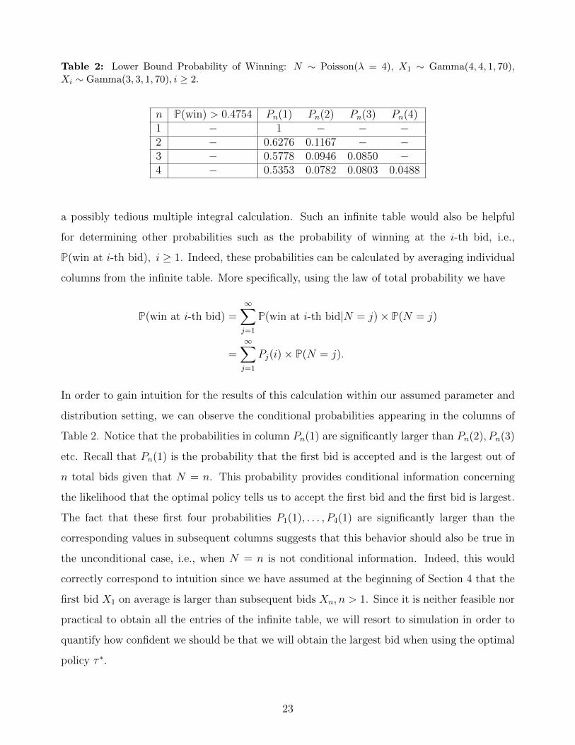
Table 2: Lower Bound Probability of Winning: N ∼ Poisson(λ = 4), X1 ∼ Gamma(4, 4, 1, 70),Xi ∼ Gamma(3, 3, 1, 70), i ≥ 2.

n P(win) > 0.4754 Pn(1) Pn(2) Pn(3) Pn(4)1 − 1 − − −2 − 0.6276 0.1167 − −3 − 0.5778 0.0946 0.0850 −4 − 0.5353 0.0782 0.0803 0.0488

a possibly tedious multiple integral calculation. Such an infinite table would also be helpful

for determining other probabilities such as the probability of winning at the i-th bid, i.e.,

P(win at i-th bid), i ≥ 1. Indeed, these probabilities can be calculated by averaging individual

columns from the infinite table. More specifically, using the law of total probability we have

P(win at i-th bid) =∞∑j=1

P(win at i-th bid|N = j)× P(N = j)

=∞∑j=1

Pj(i)× P(N = j).

In order to gain intuition for the results of this calculation within our assumed parameter and

distribution setting, we can observe the conditional probabilities appearing in the columns of

Table 2. Notice that the probabilities in column Pn(1) are significantly larger than Pn(2), Pn(3)

etc. Recall that Pn(1) is the probability that the first bid is accepted and is the largest out of

n total bids given that N = n. This probability provides conditional information concerning

the likelihood that the optimal policy tells us to accept the first bid and the first bid is largest.

The fact that these first four probabilities P1(1), . . . , P4(1) are significantly larger than the

corresponding values in subsequent columns suggests that this behavior should also be true in

the unconditional case, i.e., when N = n is not conditional information. Indeed, this would

correctly correspond to intuition since we have assumed at the beginning of Section 4 that the

first bid X1 on average is larger than subsequent bids Xn, n > 1. Since it is neither feasible nor

practical to obtain all the entries of the infinite table, we will resort to simulation in order to

quantify how confident we should be that we will obtain the largest bid when using the optimal

policy τ ∗.

23

4.2.1 Simulation

Here we discuss a monte carlo simulation of our model. We use this simulation to compare

results across different parameter assumptions for the bids. We begin with a brief description

of the simulation.

Let M be the total number of simulations. Using a random number generator, we simulate

M draws from Ni ∼ Poisson(λ), i = 1, . . .M . For each i, Ni is the number of bids in the i-th

simulation. Next, we simulate the first bid in the i-th trial: Xi,1 ∼ Gamma(4, 4, 1, 70), i =

1, . . . ,M . Finally, for each i, we simulate Ni− 1 values from Gamma(3, 3, 1, 70), At this point,

we have independently simulated all the random variables in the selling problem. Next, for

each trial, we compute τ ∗i . Note that this uses the threshold values x1, . . . , xNi which are

determined based upon Gamma(3, 3, 1, 70). Subsequently, we compute the maximum bid for

each trial, i.e., maxX1, . . . , XNi and compare this to Xτ∗i. Using this information, we can

compute the proportion of trials such that Xτ∗i= maxX1, . . . , XNi; this yields an estimate of

the probability of winning using the optimal strategy. For the j-th bid, we can compute the

proportion of trials such that τ ∗i = j and Xj is the largest of the bids in the i-th trial.

Table 3 gathers probability estimates for the overall probability of winning using τ ∗, es-

timates of the probabilities that τ ∗ = 1, 2 respectively and estimates of the probabilities of

both stopping and winning at 1, 2 respectively. We estimate these probabilities (at the 95%

confidence level) when X1 ∼ Gamma(4, 4, 1, 70), Xi ∼ Gamma(3, 3, 1, 70), i ≥ 2 and in the iid

case when Xi ∼ Gamma(3, 3, 1, 70), i ≥ 1. Additionally, we take N ∼ Poisson(λ = 4).

Table 3: Probability Estimates (m = 103 simulations): N ∼ Poisson(λ = 4), Xi ∼Gamma(3, 3, 1, 70), i ≥ 2.

P(win) P(τ∗ = 1) P(τ∗ = 2) P(1st is largest, τ∗ = 1) P(2nd is largest, τ∗ = 2)X1 ∼ Gamma(4, 4, 1, 70) 0.6960 0.6750 0.1310 0.5490 0.0770non-iid case (0.6675, 0.7245) (0.6460, 0.7040) (0.1101, 0.1519) (0.5182, 0.5798) (0.0605, 0.0935)X1 ∼ Gamma(3, 3, 1, 70) 0.5380 0.2810 0.297 0.1960 0.15iid case (0.5071, 0.5689) (0.2531, 0.3089) (0.2687, 0.3253) (0.1714, 0.2206) (0.1279, 0.1721)

Entries in the table correspond to estimates of the probability appearing in the associated

column. The first row considers the case when the first bid arrives using a different distribution

than subsequent bids. The entry corresponding to the first column in this row is the estimated

probability ≈ 69% that the seller chooses the largest of all bids offered while using the optimal

24

strategy. The corresponding entries in the second and third columns display the estimates of

the probabilities ≈ 67.5%, 13.1% that the optimal strategy tells the seller to accept the first and

second bid respectively. Finally the fourth and fifth columns present the probability estimates

≈ 54.9%, 7.7% that the optimal strategy tells the seller to accept the first or second bid and it

is, in fact, the largest of all presented bids. The second row presents the probability estimates

when all bids come from the same distribution, i.e., the iid case. Intervals below estimates are

95% confidence intervals.

The results in Table 3 comply with intuition. We find that the probability of accepting the

largest bid using the optimal strategy is approximately 69%. Compare this to the lower bound

47.54% we determined in Table 2. We note that this is substantially larger than the iid case

where the probability is approximately 53%.

Remark 4. From Table 3, we see that if, on average, the first bid is larger than subsequent

bids, then the optimal strategy produces a greater likelihood of success. This is primarily due

to the fact that the threshold x1 does not change across the non-iid and iid cases. Thus, larger

than average first bids increases the likelihood that the seller both accepts the first bid and the

first bid is the largest of all bids. This is demonstrated in the fifth column of the table; compare

54.9% non-iid and 19.6% iid.

Table 3 also shows the impact that the optimal strategy has on the likelihood of success

across the two cases. More specifically, in the non-iid case, the probability of the event that

the optimal strategy indicates to accept an offer and it is, in fact, the largest of all bids is

significantly larger for the first bid relative to the second bid. This implies that the seller has

much greater confidence that the accepted bid is the largest bid when τ ∗ = 1 than when τ ∗ = 2.

This makes good intuitive sense in the non-iid case since the first bid is, on average, larger but

it is also interestingly true in the iid case; compare 19.6% and 15%.

This result of our theoretical model is in line with the empirical result of Merlo and Ortalo-

Magne (2004) who report that approximately 72% of all the transactions in their data set occur

within the first match, and only 10% of all sales occur after three or more matches. Note also

from Table 3 that the probability of accepting the first bid in our model is much closer to the

72% probability reported in Merlo and Ortalo-Magne (2004) for the non-iid case than for the

iid case, hence providing support for the property of our model that the distribution of the first

25

bid is different from the distribution of the subsequent bids.

4.3 Likelihood of a Sale

In this paper, we incorporate into a real estate selling model the realistic risk facing the seller

that if she rejects a current offer, there may be no future offers to entertain. Notice, if N ∼

Pois(λ), then there is a positive probability that time-on-the-market is infinite since P(N =

0) = e−λ > 0. As such, there is a nonzero possibility that the seller may not have any bids to

entertain. Within such a modeling framework, the expected time-on-the-market is unhelpful

information since it is infinite. Instead, we consider the likelihood that the asset is sold, i.e.,

P(τ ∗ <∞). This gives us the probability that the seller is offered a bid for the real estate asset

and she accepts it at some point.

Using the optimal strategy we have identified, we calculate the probability that a sale occurs

for alternative arrival rate of offers. An increase in the number of offers might be caused by a

change in mortgage rates, GDP, supply of new units, or property taxes. Sample estimates and

95% confidence intervals of the probability of a sale under different arrival rates are reported

in Table 4.

Table 4: Sample values for P(τ∗ < ∞), m = 104 simulations: N ∼ Poisson(λ), X1 ∼Gamma(4, 4, 1, 70), Xi ∼ Gamma(3, 3, 1, 70), i ≥ 2. We use z97.5 since m = 104 is large and σ isthe unbiased sample standard deviation.

λ P(τ ∗ <∞) 95% Confidence Interval: τ ∗ ± z97.5σ/√m

1 0.6323 (0.622849,0.641751)2 0.8315 (0.824163,0.838837)3 0.8342 (0.82691,0.84149)4 0.8167 (0.809116,0.824284)5 0.7963 (0.788406, 0.804194)

Table 4 shows an interesting trade off when it comes to the probability of a sale and the

arrival rate of bids.

Remark 5. A higher number of bids can cause a decrease as well as an increase in the proba-

bility of a sale.

26

Prior to viewing the results, one might be inclined to believe that the probability of a sale

occurring must be higher for a higher average number of bids. Surprisingly, this intuition is not

necessarily true. Indeed, Table 4 highlight the delicate balance between the mean number of bids

λ and the seller’s optimal threshold acceptance values. Notice that when the average number

of bids increases from λ = 2 to λ = 3, the first three threshold values for the seller increase

from 75.8466, 70, 70 to 79.2731, 76.6714, 73.1019, respectively. Knowledge of a higher average

number of bids induces higher threshold values. These higher thresholds, in turn, decrease the

likelihood of a sale taking place. This serves as an explanation for a lower sale probability in

light of an increase in average number of bids, e.g., compare λ = 3; P(τ ∗ < ∞) = 0.8342 with

λ = 4; P(τ ∗ <∞) = 0.8167.

5 Conclusion

In this paper, we have analyzed the problem of a seller who seeks to maximize the probability

of accepting the largest bid. The bids are random draws from a known distribution and the

seller has to decide after each draw whether or not to accept the bid or wait for the arrival of

a new bid.

Our contribution to the existing literature is two-fold. One is that we recognize that in

many markets the seller has to decide whether to accept or reject a bid without knowing

whether another bid would arrive. This is a departure from standard search models where the

seller can always obtain another bid by incurring a search cost. The other contribution of our

paper is that we consider the possibility that the first bid is distributionally different from all

subsequent bids. This property of our model captures anecdotal evidence that first bids on real

estate property tend to be larger than subsequent bids.

In this more complicated set up, we are able to solve for a simple optimal strategy for the

seller. A distinguishing feature of our optimal strategy is its stochastic nature. In classical search

theory, the optimal strategy is characterized by a deterministic non-increasing set of reservation

prices. Within our framework, reservation prices are no longer deterministic. Rather, the

optimal decision to accept a bid requires not only that the bid exceeds a certain threshold level,

but it also needs to be greater than all past (random) bids received. In addition, we are able

to calculate the probability of accepting the highest bid, estimate a confidence interval for this

27

probability and show how it changes as the seller rejects a bid and waits for the arrival of a

new bid. We also show than an improvement in market conditions that leads to a rise in the

expected number of bids can lead to a decrease as well as to an increase in the probability of a

sale.

28

A Appendix: Embedding within Prospect Theory?

Suppose there are three sequential offers for an asset which arrive independently and are uni-

formly distributed over the unit interval, i.e.,

Xi ∼ Unif[0, 1], i = 1, 2, 3.

Within this setup, we determine that the threshold values are x1 = 0.6898, x2 = 0.5, x3 = 0.

The optimal policy is

τ ∗ = infn : Xn = maxX1, . . . , Xn and Xn ≥ xn.

In words, the seller accepts the first offer which is both the largest of what has been previously

offered and is at least as large as the threshold. Let yi denote a realization of the i-th offer. If

the first offer y1 is rejected (i.e., y1 < x1), then any smaller second offer (i.e., y2 < y1) will also

be rejected even if y2 exceeds the required threshold (i.e., y2 ≥ x2). This represents a “past

offer regret” in which the seller makes a decision not to sell because it represents a loss relative

to what they could have sold the property at if they accepted the first offer. See Figure 3 for a

æ

æ

æ

ò

ò

ò

0.5 1.0 1.5 2.0 2.5 3.0

0.2

0.4

0.6

0.8

1.0

Bid_Amount

ò Bid

æ Threshold

Figure 3: Second bid is not accepted since it represents a “loss”.

visual illustration of this policy.

In order to see if we can embed our analysis within prospect theory, we consider the following

situation: Suppose the first offer y1 has been rejected and the seller must decide whether or not

to accept the second offer y2. We seek a modified utility function (i.e., monotonically increasing,

convex for losses, concave for gains etc) which satisfies the conditions of our optimal policy.

The three conditions that U(·) must satisfy are:

29

1. E[U(X3 − y1)] ≥ U(y2 − y1), for any y2 ≤ y1,

2. E[U(X3 − y2)] ≥ U(y2 − y1), for any y1 < y2 and y2 < 0.5.

3. E[U(X3 − y2)] ≤ U(y2 − y1), for any y1 < y2 and y2 ≥ 0.5.

In words, condition (1) says that the seller always prefers to wait for the third bid if the second

offer is lower than the first offer. The value X3− y1 represents the gain/loss of taking the third

offer when y1 ≥ y2. Condition (2) states that the seller always prefers to wait for the third bid

when the second offer does not exceed the threshold x2 = 0.5 even when there is a guaranteed

perceived gain y2 > y1. The value X3 − y2 represents the gain/loss of taking the third offer

when y1 < y2. Finally, condition (3) states that the seller prefers to accept y2 for the property

(with perceived gain of y2 > y1) when it meets or exceeds the threshold x2 = 0.5 and is larger

than the first offer y1.

Since (1) needs to hold for any y2 ≤ y1, we must require that U(z) = −∞ for z < 0. If

this property of U(·) did not hold, then we could always find y2 close enough to y1 such that

E[U(X3 − y1)]− U(y2 − y1) < 0. Intuitively, the restriction U(z) = −∞ for z < 0 corresponds

to infinite loss aversion for the seller since it is optimal for the seller to never sell if there’s a

loss. Next, notice that condition (2) requires E[U(X3 − y2)] > 0 when y1 < y2 < 0.5. But since

U(z) = −∞ for z < 0 and P[X3 − y2 < 0] > 0, it must hold that E[U(X3 − y2)] = −∞, a

contradiction. Thus, we cannot find a function U(·) such that we can embed our model within

prospect theory.

B Appendix: Technical Discussion Regarding Optimal

Policy

The purpose of this section is to provide technical details sufficient for determining the optimal

policy to our problem. It follows Porosinski (1987) and culminates in Theorem 1 in Section 3).

Find the stopping time τ ∗ satisfying

E(n,x)[f0(τ ∗, Xτ∗)] = supσ≥n

E(n,x)[f0(σ,Xσ)] =: s0(n, x),(P’)

30

where E(n,x) denotes the expected value with respect to P(n,x)(·) = p(n, x; ·). From the general

theory of optimal stopping (e.g. Shiryaev (1979)), it is known that s0(n, x) satisfies

s0(n, x) = maxf0(n, x), P0s0(n, x),where

P0h(e) =

∫Eh(a)Pe(da),

(7)

for a bounded function h : E→ R. If we assume that h(δ) = 0, then P0h(δ) = 0 and from (1),

we have

P0h(n, x) =∞∑

m=n+1

∫ ∞x

h(m, y)

(πmπn

)(F (x))m−n−1 dF (y).

Definition 1. The set 4 := e ∈ E : s0(e) = f0(e) is known as the stopping set.

Again, from general theory of optimal stopping, we know that the stopping time τ0 :=

infn ∈ N : Yn ∈ 4 is optimal only if τ0 < ∞ almost surely, i.e., with probability one. Note

that since our Markov chain attains the state δ almost surely (note f0(δ) = 0 = s0(δ)), we can

conclude that τ0 is optimal for (P’). Thus, an investigation into the stopping set 4 will lead to

an understanding of the optimal strategy. To simplify notation, let

f(n, x) = πnf0(n, x) =∞∑m=n

pm(F (x))m−n,

s(n, x) = πns0(n, x).

Transforming (2), we have

s(n, x) = maxf(n, x), Ps(n, x), (8)

where

Ps(n, x) =∞∑

m=n+1

∫ ∞x

s(m, y) (F (x))m−n−1 dF (y).

31

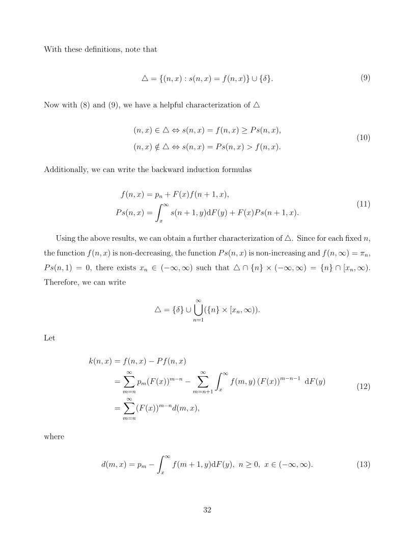
With these definitions, note that

4 = (n, x) : s(n, x) = f(n, x) ∪ δ. (9)

Now with (8) and (9), we have a helpful characterization of 4

(n, x) ∈ 4 ⇔ s(n, x) = f(n, x) ≥ Ps(n, x),

(n, x) /∈ 4 ⇔ s(n, x) = Ps(n, x) > f(n, x).(10)

Additionally, we can write the backward induction formulas

f(n, x) = pn + F (x)f(n+ 1, x),

Ps(n, x) =

∫ ∞x

s(n+ 1, y)dF (y) + F (x)Ps(n+ 1, x).(11)

Using the above results, we can obtain a further characterization of4. Since for each fixed n,

the function f(n, x) is non-decreasing, the function Ps(n, x) is non-increasing and f(n,∞) = πn,

Ps(n, 1) = 0, there exists xn ∈ (−∞,∞) such that 4 ∩ n × (−∞,∞) = n ∩ [xn,∞).

Therefore, we can write

4 = δ ∪∞⋃n=1

(n × [xn,∞)).

Let

k(n, x) = f(n, x)− Pf(n, x)

=∞∑m=n

pm(F (x))m−n −∞∑

m=n+1

∫ ∞x

f(m, y) (F (x))m−n−1 dF (y)

=∞∑m=n

(F (x))m−nd(m,x),

(12)

where

d(m,x) = pm −∫ ∞x

f(m+ 1, y)dF (y), n ≥ 0, x ∈ (−∞,∞). (13)

32

Notice that k(n, x) ≥ 0 for (n, x) ∈ 4. In what follows, shall see that the values of c(n, x) are

an important determinant of the structure of 4. Given the relationship between k(n, x) and

d(n, x), an understanding of the structure of d(n, x) will assist in the characterization of 4. We

can begin an investigation into the function d(n, x) by understanding its interaction with 4

when fixing one of its parameters. Indeed, for fixed x ∈ (−∞,∞), consider the x-cross section

4(x) := n ∈ N : (n, x) ∈ 4.

Definition 2. Letting d(−1, x) := −1, we say that (d(n, x))∞n=−1 changes sign at the point m

if d(m,x) ≥ 0 and d(m− 1, x) < 0 (i.e., an up-crossing).

If we consider situations when, for each fixed x ∈ (−∞,∞), the number of sign changes of

(d(n, x))∞n=−1 equals 1, we are then able to relate the optimal stopping time for (P’) to the first

entrance time of the Markov chain Y into a closed subset in E. Instances when (d(n, x))∞n=−1

changes sign only once are referred to as monotone cases. Below, we consider three distributions

with the monotone property and prove the optimal strategy for the seller.

B.1 Monotone Cases

B.1.1 One-Point Distribution.

In this situation, we suppose P(N = n) = 1. Then, d(k, x) < 0 for k < n, d(n, x) > 0 and

d(k, x) = 0 for k > n. Thus, (d(k, x))∞k=−1 changes sign exactly once.

B.1.2 The Uniform Distribution on 1, 2, . . . , n.

Note that in this case, d(0, x) < 0, d(n, x) = 1/n, d(k, x) = 0 for k > n and the sequence

(d(k, x))nk=1 is increasing since for 1 ≤ k ≤ n,

d(k, x) =1

n

(1−

∫ ∞x

n∑i=k+1

[F (y)]i−(k+1)dF (y)

)=

1

n

1−∫ ∞x

n−(k+1)∑i=0

[F (y)]idF (y)

.

Thus, (d(k, x))∞k=−1 changes sign exactly once.

33

B.1.3 Poisson Distribution with parameter λ.

For 1 ≤ k ≤ n, we have

d(k, x) =λk

k!e−λ −

∫ ∞x

∞∑i=k+1

λi

i!e−λ[F (y)]i−(k+1)dF (y).

If we assume that F is absolutely continuous, then using integration by parts (to obtain the

second equality below) we have

d(k, x) =λk

k!e−λ −

∫ ∞x

∞∑i=k+1

λi

i!e−λ[F (y)]i−(k+1)dF (y)

=λk

k!e−λ −

∞∑i=k+1

λi

i!e−λ

1

i− k(1− [F (x)]i−k)

=λk

k!e−λ(1− a(k, x)), where

a(k, x) :=∞∑i=1

λik!

(i+ k)!i(1− [F (x)]i).

Since a(k, x) is a decreasing function of k for fixed x, we can conclude that (d(k, x))∞k=−1 changes

sign exactly once.

B.2 Optimal Stopping under Monotone Case

The following lemma presented in Porosinski (1987) provides a solution to our problem and

will be instrumental in proving Theorem 1 of our paper.

Lemma 1. Let Y = (Yn)∞n=1 be a homogeneous Markov chain on (Ω,F ,P) with state space

(E,P) and let p(e;B) = P(Yn+1 ∈ B|Yn = e) for B ∈ B. Let f0 : E→ R be a bounded function.

Let

Γ := e ∈ E : f0(e) ≥ P0f0(e),

σΓ := infn : Yn ∈ Γ,

where P0 is defined in (2). If

(i) p(e; Γ) = 1 for e ∈ Γ,

34

(ii) σΓ <∞ almost surely,

then σΓ is an optimal stopping time for Y with reward f0.

We are now in a position to prove the optimal strategy of Theorem 1 for our paper.

Theorem. If Assumption 1 holds and the sequence (d(k, n))∞k=−1 changes sign once for each

fixed x, then the solution to (P) exists and the stopping time

τ ∗ = infn : Xn = maxX1, . . . , Xn and Xn ≥ xn, (14)

is optimal for (P) where xn is the least root of the equation k(n, x) = 0 in [R,∞), for each

n ∈ N. Moreover, the sequence (xn)∞n=1.

Proof. This proof proceeds as in the proof of Theorem 2 in Porosinski (1987) but we include

it here for completeness. Note that Γ = e ∈ E : f0(e) ≥ P0f0(e) and (n, x) ∈ Γ is equivalent

to k(n, x) ≥ 0. Suppose that d(n, x) ≥ 0. Then d(n, y) ≥ 0 for y ≥ x because d(n, x) is

a non-decreasing function (see (13)) for n fixed. Using the monotone property, the sequence

d(h, y), for each y, changes sign at most once which implies that d(h, y) ≥ 0 for h ≥ n and

y ≥ x. Then, by (12) k(h, x) ≥ 0, i.e., (h, x) ∈ Γ for h ≥ n and y ≥ x. Hence, k(h, y) ≥ 0 or

equivalently (h, y) ∈ Γ for h ≥ n and y ≥ x.

Now we show that k(n, x) ≥ 0 implies k(n, y) ≥ 0 for y ≥ x. Let k(n, x) ≥ 0. Since

k(n,∞) = πn ≥ 0, there exists an x such that k(n, x) ≥ 0. Now suppose there exists y > x

such that k(n, y) < 0. Then, it must be the case that d(n, y) < 0 (since (n, y) ∈ Γ otherwise as

shown above) and hence d(n, x) < 0 also, since d(n, ·) is non-decreasing.

Let d(m,x) < 0 for m = n, . . . , n+ s and d(n+ s+ 1, x) ≥ 0 for some s ≥ 0. From (12), we

know that

k(n, x) = d(n, x) + F (x)k(n+ 1, x). (15)

Since k(n, x) ≥ 0 and d(n, x) < 0, we know from above that k(n + 1, x) > 0. Repeating this

iteratively for values k(n+ 2, x), . . . , k(n+ s, x), we obtain

k(n+ s, x) = d(n+ s, x) + F (x)d(n+ s+ 1, x) + (F (x))2d(n+ s+ 2, x) + · · · > 0.

35

Recall that d(h, y) is a nondecreasing function for each h. Additionally, d(h, x) ≥ 0 for h ≥

n+ s+ 1 (notice this uses the monotonicity assumption here). Hence,

0 < k(n+ s, x) ≤ k(n+ s, y),

k(n+ s− 1, x) ≤ d(n+ s− 1, x) + xk(n+ s, y) ≤ k(n+ s− 1, y).

Now repeating this operation several times yields k(n, x) ≤ k(n, y) which is a contradiction to

our supposition that k(n, y) < 0. Thus, we have k(n, x) ≥ 0 for x ≤ xn and k(n, x) < 0 for

x < xn where xn = infx : k(n, x) ≥ 0. Since δ ∈ Γ, we can conclude that Γ has the form

Γ = δ ∪∞⋃n=1

n × [xn,∞).

We now show that (xn)∞n=1 is non-increasing. It suffices to show that (n, x) ∈ Γ implies

(n + 1, x) ∈ Γ for each n ∈ N and x ∈ [R,∞). Assume that k(n, x) ≥ 0. If d(n, x) ≥ 0, then

d(n + 1, x) ≥ 0 also and thus (n + 1, x) ∈ Γ. If d(n, x) < 0, then from (15), we have that

k(n+ 1, x) > 0 and hence (n+ 1, x) ∈ Γ. Therefore, (xn)∞n=1 is non-increasing.

Now, since (xn)∞n=1 is non-increasing along with the fact that our Markov chain Y “goes to

the right and upward” we know that assumption (i) of Lemma 1 holds. Additionally, since Y

attains the state δ almost surely, we also know that assumption (ii) of Lemma 1 holds. Thus,

we can apply the lemma and the proof concludes.

C Appendix: Numerical Results: One-point and Uni-

form total bids

In our paper, we examined optimal strategy under the assumption that the number of bids

was Poisson distributed. Here, we characterize the optimal strategy τ ∗ and the probability of

accepting the largest bid offer when: N ∼ One-pointn and N ∼ Uniform1, . . . , n.

36

C.1 One-point distributed total bids

C.1.1 Threshold values: xn

Here, we suppose that P[N = n] = 1. From Section B.1.1, we can apply Theorem ?? and

calculate the optimal threshold offer, 1 ≤ k ≤ n using dk = F−1(bk), where bk := un−(k−1)

and ui is the threshold for the i-th bid when the bids are uniformly distributed. Gilbert and

Mosteller (1966) provide approximations for bi (which is independent of n) for which we use to

obtain values in Table 5 below. Note that dk = xn−(k−1), k = 1, . . . , n.

Table 5: Optimal Decision Offers: N ∼ One point(n), X1 ∼ Gamma(4, 4, 1, 70), Xi ∼Gamma(3, 3, 1, 70), i ≥ 2.

k 1 2 3 4 5 6 7 8 9 10

dk 70 78.0222 80.6765 82.2927 83.4513 84.3524 85.0884 85.7097 86.2468 86.71960

According to Table 5, we only accept a bid Xn if it is at least as big as both dn and what has

already been presented. Note that we only accept a bid Xk if it is at least as big as both dn−k+1

and what has already been presented. For example, when presented with the second-to-last

bid (i.e., Xn−1 has been presented) the optimal threshold value is d2 = 78.0222. Thus, we only

accept Xn−1 if it is at least the median of the distribution of the final bid Xn. Notice that the

distribution F1 plays no role in determining d2.

C.1.2 Probability of accepting the largest bid

Here, we use equation (6) to obtain in Table 6 the probability of accepting the largest bid when

the number of bids is known with certainty to be n = 1, 2, 3, and 4.

Table 6: Probability of Winning: N ∼ One− point(n), X1 ∼ Gamma(4, 4, 1, 70), Xi ∼Gamma(3, 3, 1, 70), i ≥ 2.

n P(win) Pn(1) Pn(2) Pn(3) Pn(4)1 1 1 − − −2 0.8311 0.7331 0.0980 − −3 0.7637 0.5946 0.0968 0.0723 −4 0.7247 0.5113 0.0806 0.0792 0.0537

37

C.2 Uniformly distributed total bids

C.2.1 Threshold values: xn

Here, we consider the case when the number of bids N is uniformly distributed on 1, 2, . . . , n,

i.e., pk = 1/n for k = 1, 2, . . . , n. From Section B.1.2, we can apply Theorem 1 and calculate

the optimal threshold offer.

Table 7: Optimal Decision Offers dn: N ∼ Uniform(1, 2, . . . , n), X1 ∼ Gamma(4, 4, 1, 70), Xi ∼Gamma(3, 3, 1, 70), i ≥ 2.

k 1 2 3 4 5 6 7 8 9 10

dk 70 70 75.6291 77.5764 78.9053 79.9153 80.73 81.4111 81.996 82.5108

Again, we can calculate the optimal threshold offer, 1 ≤ k ≤ n using dk = F−1(bk), where

bk := un−(k−1) and ui is the threshold for the i-th bid when the bids are uniformly distributed.

Porosinski (1987) page 305 shows that bk is independent of n. As in the one-point distribution

case, we only accept a bid Xk if it is at least as big as both dn−k+1 and what has already

been presented. Notice that when at most one bid remains (i.e., Xn−1 has been presented) the

optimal threshold value is d2 = 70. This may seem counterintuitive at first but is true due

to the fact that, when N is uniformly distributed, there is a possibility that N equals n − 1,

i.e., Xn−1 may be the last bid presented. For a given value of Xn−1, say x, the event that x is

the largest of the bids can result from there being no future bids or it can result from it being

larger than the final bid (if there is one). This effectively lowers the threshold below its value

when N has a one-point distribution.

C.2.2 Probability of accepting the largest bid

Here, we use equation (6) to obtain in Table 8 the probability of accepting the largest bid when

the number of bids is uniformly distributed between 1 and n with n = 1, 2, 3, and 4.

38

Table 8: Probability of Winning: N ∼ Uniform(1, 2, . . . , n), X1 ∼ Gamma(4, 4, 1, 70), Xi ∼Gamma(3, 3, 1, 70), i ≥ 2.

n P(win) Pn(1) Pn(2) Pn(3) Pn(4)1 1 1 − − −2 0.8895 0.7790 0 − −3 0.8240 0.6591 0.0262 0.0077 −4 0.7784 0.5797 0.0396 0.0133 0.0088

References

Anenberg, Elliot, 2012, Information frictions and housing market dynamics, Working paper,

Board of Governors of the Federal Reserve System (US).

Brown, Keith C, and Deborah J Brown, 1986, Using order statistics to estimate real estate bid

distributions, Management science 32, 289–297.

Chow, Y. S., Herbert Robbins, and David Siegmund, 1971, Great expectations: the theory of

optimal stopping. Houghton Mifflin Co.

Freeman, PR, 1983, The secretary problem and its extensions: A review, International Statis-

tical Review/Revue Internationale de Statistique pp. 189–206.

Gilbert, John P., and Frederick Mosteller, 1966, Recognizing the maximum of a sequence, J.

Amer. Statist. Assoc. 61, 35–73.

Guttman, Irwin, 1960, On a problem of L. Moser, Canad. Math. Bull. 3, 35–39.

Knight, John R, 2002, Listing price, time on market, and ultimate selling price: Causes and

effects of listing price changes, Real estate economics 30, 213–237.

Lancaster, Tony, and Andrew Chesher, 1983, An Econometric Analysis of Reservation Wages,

Econometrica 51, 1661–76.

Lippman, Steven A, and John J McCall, 1976, The Economics of Job Search: A Survey,

Economic Inquiry 14, 347–68.

39

Merlo, Antonio, and Francois Ortalo-Magne, 2004, Bargaining over residential real estate: evi-

dence from England, Journal of Urban Economics 56, 192–216.

Miller, Norman G, and Michael A Sklarz, 1986, A Note On Leaning Indicators Of Housing

Market Price Trends, Journal of Real Estate Research 1, 99–109.

Moser, Leo, 1956, On a Problem of Cayley, Scripta Mathematica 22, 289–292.

Porosinski, Zdzis law, 1987, The full-information best choice problem with a random number of

observations, Stochastic Process. Appl. 24, 293–307.

Salant, Stephen W, 1991, For sale by owner: When to use a broker and how to price the house,

The Journal of Real Estate Finance and Economics 4, 157–173.

Shiryaev, A. N., 2008, Optimal stopping rules. vol. 8 of Stochastic Modelling and Applied Prob-

ability. Springer-Verlag.

Sirmans, Stacy G, David A Macpherson, and Emily N Zietz, 2005, The composition of hedonic

pricing models, Journal of Real Estate Literature 13, 1–44.

Stigler, George J., 1961, The Economics of Information, Journal of Political Economy 69, 213.

Taylor, Curtis R, 1999, Time-on-the-Market as a Sign of Quality, The Review of Economic

Studies 66, 555–578.

Tryfos, Peter, 1981, On the Estimation of Bid Distributions in Real Estate Markets, Manage-

ment Science 27, 587–601.

van den Berg, Gerard J, 1990, Nonstationarity in Job Search Theory, Review of Economic

Studies 57, 255–77.

Yavas, Abdullah, and Shiawee Yang, 1995, The strategic role of listing price in marketing real

estate: theory and evidence, Real Estate Economics 23, 347–368.

40