first-order and second-order statistical analysis of 3d and 2d

First-order and Second-order Statistical Analysis of 3D and2D Image Structure

S Kalkan†, F Worgotter† and N Kruger‡

† Bernstein Centre for Computational Neuroscience, University of Gottingen, Germany‡ Cognitive Vision Group, University of Southern Denmark, Denmark

E-mail: sinan,[email protected], [email protected]

Abstract. In the first part of this paper, we analyze the relation between local imagestructures (i.e., homogeneous, edge-like, corner-like or texture-like structures) and theunderlying local 3D structure (represented in terms of continuous surfaces and differentkinds of 3D discontinuities) using range data with real-world color images. We find thathomogeneous image structures correspond to continuous surfaces, and discontinuities aremainly formed by edge-like or corner-like structures, which we discuss regarding potentialcomputer vision applications and existing assumptions about the 3D world.

In the second part, we utilize the measurements developed in the first part to investigatehow the depth at homogeneous image structures is related to the depth of neighbor edges. Forthis, we first extract the local 3D structure of regularly sampled points, and then, analyze thecoplanarity relation between these local 3D structures. We show that the likelihood to find acertain depth at a homogeneous image patch depends on the distance between the image patchand a neighbor edge. We find that this dependence is higher when there is a second neighboredge which is coplanar with the first neighbor edge. These results allow deriving statisticallybased prediction models for depth interpolation on homogeneous image structures.

Author Posting. (c) Taylor & Francis, 2007.This is the author’s version of the work. It is posted here by permission of Taylor &Francis for personal use, not for redistribution. The definitive version was publishedin Network: Computation in Neural Systems, Volume 18 Issue 2, January 2007.doi:10.1080/09548980701580444 (http://dx.doi.org/10.1080/09548980701580444)

First-order and Second-order Statistical Analysis of 3D and 2D Image Structure 2

1. Introduction

Depth estimation relies on the extraction of 3D structure from 2D images which is realized bya set of inverse problems including structure from motion, stereo vision, shape from shading,linear perspective, texture gradients and occlusion [Bruce et al., 2003]. In methods whichmake use of multiple views (i.e., stereo and structure from motion), correspondences betweendifferent 2D views of the scene are required. In contrast, monocular or pictorial cues suchas shape from shading, texture gradients or linear perspective use statistical and geometricalrelations within one image to make statements about the underlying 3D structure.

Many surfaces have only weak texture or no texture at all, and as a consequence, thecorrespondence problem is very hard or not at all resolvable for these surfaces. Nevertheless,humans are able to reconstruct the 3D information for these surfaces, too. This gives riseto the assumption that in the human visual system, an interpolation process is realised that,starting with the local analysis of edges, corners and textures, computes depth also in areaswhere correspondences cannot easily be found.

Processing of depth in the human visual system starts with the processing of localimage structures (such as edge-like structures, corner-like structures and textures) in V1[Hubel and Wiesel, 1969, Gallant et al., 1994, Lee et al., 1998]. These structures (called 2Dstructures in the rest of the paper) are utilized in stereo vision, depth from motion, depth fromtexture gradients and other depth cues, which are localized in different parts of the brain,starting from V1 and involving V2, V3, V4 and MT (see, e.g., [Sereno et al., 2002]).

There exists good evidence that depth cues which are not directly based oncorrespondences evolve rather late in the development of the human visual system.For example, pictorial depth cues are made use of only after approximately 6 months[Kellman and Arterberry, 1998]. This indicates that experience may play an important role inthe development of these cues, i.e., that we have to understand depth perception as a statisticallearning problem [Knill and Richards, 1996, Rao et al., 2002, Purves and Lotto, 2002]. Astep towards such an understanding is the investigation and use of the statistical relationsbetween the local 2D structures and the underlying 3D structure for each of these depth cues[Knill and Richards, 1996, Rao et al., 2002, Purves and Lotto, 2002].

With the notion that the human visual system is adapted to the statistics ofthe environment [Brunswik and Kamiya, 1953, Knill and Richards, 1996, Krueger, 1998,Olshausen and Field, 1996, Rao et al., 2002, Purves and Lotto, 2002, Simoncelli, 2003] andits successful applications to grouping, object recognition and stereo [Elder and Goldberg, 2002,Elder et al., 2003, Pugeault et al., 2004, Zhu, 1999], the analysis and the usage of natural im-age statistics have become an important focus of vision research. Moreover, with the advancesin technology, it has been also possible to analyze the 3D world using 3D range scanners[Howe and Purves, 2004, Huang et al., 2000, Potetz and Lee, 2003, Yang and Purves, 2003].

In this paper, we analyze first-order and second-order relations‡ between 2D and 3D

‡ In this paper, a relation is first-order if it involves two entities and an event between them. Analogously, arelation is second-order if there are three entities and (at least) two events between them.


structures extracted from chromatic 3D range data§. For the first-order analysis, we investigatethe relation between local 2D structures (i.e., homogeneous, edge-like, corner-like or texture-like structures) and the underlying local 3D structure. As for the second-order analysis, weinvestigate the relation between the depth at homogeneous 2D structures and the depth at thebounding edges.

There have been only a few studies that have analyzed the 3D world from range data[Howe and Purves, 2004, Huang et al., 2000, Potetz and Lee, 2003, Yang and Purves, 2003],and these works have only been first-order. In [Yang and Purves, 2003], the distribution ofroughness, size, distance, 3D orientation, curvature and independent components of surfaceswas analyzed. Their major conclusions were: (1) local 3D patches tend to be saddle-like,and (2) natural scene geometry is quite regular and less complex than luminance images.In [Huang et al., 2000], the distribution of 3D points was analyzed using co-occurrencestatistics and 2D and 3D joint distributions of Haar filter reactions. They showed thatrange images are much simpler to analyze than optical images and that a 3D scene iscomposed of piecewise smooth regions. In [Potetz and Lee, 2003], the correlation betweenlight intensities of the image data and the corresponding range data as well as surfaceconvexity were investigated. They could justify the event that brighter objects are closerto the viewer, which is used by shape from shading algorithms in estimating depth. In[Howe and Purves, 2002, Howe and Purves, 2004], range image statistics were analyzed forexplanation of several visual illusions.

Our first-order analysis differs from these works. For 2D local image patches, existingstudies have only considered light intensity. As for 3D local patches, the most complexconsidered representation has been the curvature of the local 3D patch. In this work, however,we create a higher-order representation of the 2D local image patches and the 3D localpatches; we represent 2D local image patches using homogeneous, edge-like, corner-like ortexture-like structures, and 3D local patches using continuous surfaces and different kinds of3D discontinuities. By this, we relate established local 2D structures to their underlying 3Dstructures.

For the first-order analysis, we compute the conditional likelihood P (3D Structure | 2D Structure),by creating 2D and 3D representations of the local structure. Using this likelihood, we quan-tify some assumptions made by the studies that reconstruct the 3D world from dense rangedata. For example, we will show that the depth distribution varies significantly for differentvisual features, and we will quantify already established inter-dependencies such as ’no newsis good news’ [Grimson, 1983]. This work also supports the understanding of how intrinsicproperties of 2D–3D relations can be used for the reconstruction of depth, for example, byusing statistical priors in the formalisation of depth cues.

For the second-order analysis, given two proximate co-planar edges, we computethe ’likelihood field’ of finding co-planar surface patches which project as homogeneous2D structures in the 2D image. This likelihood field is similar to the ’associationfield’ [Field et al., 1993] which is a likelihood field also based on natural image statistics.

§ In this paper, chromatic 3D range data means range data which has associated real-world color information.The color information is acquired using a digital camera which is calibrated with the range scanner.


The ’likelihood field’ which we compute provides important information about (1) thepredictability of depth at homogeneous 2D structures using the depth available at the boundingedges and (2) the relative complexity of 3D geometric structure compared to the complexityof local 2D structures.

The paper is organized as follows: In sections 2 and 3, we define the types of local 2Dstructures and local 3D structures and how we extract them for our analysis. In section 4, weanalyze the relation between the local 2D and 3D structures, and discuss the results. In section5, we present our methods for analyzing the second-order relation between the homogeneous2D structures and bounding edge structures, and discuss the results. Finally, we conclude thepaper in section 6 with a discussion.

2. Local 2D Structures

Figure 1. How a set of 54 patches map to the different areas of the intrinsic dimensionalitytriangle. Some examples from these patches are also shown. The horizontal and verticalaxes of the triangle denote the contrast and the orientation variances of the image patches,respectively.

We distinguish between the following local 2D structures (examples of each structure isgiven in figure 1):

• Homogeneous 2D structures: Homogeneous 2D structures are signals of uniformintensities, and they are not much made use of in the human visual system because retinalganglion cells give only weak sustained responses and adapt quickly at homogeneousintensities [Bruce et al., 2003].

• Edge–like 2D structures: Edges are low-level structures which constitute theboundaries between homogeneous or texture-like signals. Detection of edge-like


structures in the human visual system starts with orientation sensitive cells in V1[Hubel and Wiesel, 1969], and biological and machine vision systems depend on theirreliable extraction and utilization [Marr, 1982, Koenderink and Dorn, 1982].

• Corner-like 2D structures: Corners‖ are image patches where two or more edge-likestructures with significantly different orientations intersect (see, e.g., [Guzman, 1968,Rubin, 2001] for their importance in vision). It has been suggested that the humanvisual system makes use of them for different tasks like recovery of surface occlusion[Guzman, 1968, Rubin, 2001] and shape interpretation [Malik, 1987].

• Texture-like 2D structures: Although there is not a widely-agreed definition, textures areoften defined as signals which consist of repetitive, random or directional structures (fortheir analysis, extraction and importance in vision, see e.g., [Tuceryan and Jain, 1998]).Our world consists of textures on many surfaces, and the fact that we can reliablyreconstruct the 3D structure from any textured environment indicates that human visualsystem makes use of and is very good at the analysis and the utilization of textures.In this paper, we define texture as 2D structures which have low spectral energy and a lotof orientation variance (see figure 1 and section 2.1).

It is locally hard to distinguish between these ’ideal’ cases, and there are 2D structuresthat carry mixed properties of these ’ideal’ cases. The classification of the features outlinedabove is a discrete one. However, a discrete classification may cause problems as the inherentproperties of the ”mixed” structures are lost in the discretization process. Instead, in this paper,we make use of a continuous scheme which is based on the concept of intrinsic dimensionality(see section 2.1 for more details).

2.1. Detection of Local 2D Structures

In image processing, intrinsic dimensionality (iD) was introduced by [Zetzsche and Barth, 1990]and was used to formalize a discrete distinction between edge-like and junction-like struc-tures. This corresponds to a classical interpretation of local 2D structures in computer vision.

Homogeneous, edge-like and junction-like structures are respectively classified by iD asintrinsically zero dimensional (i0D), intrinsically one dimensional (i1D) and intrinsically twodimensional (i2D).

When looking at the spectral representation of a local image patch (see figure 2(a,b)), wesee that the energy of an i0D signal is concentrated in the origin (figure 2(b)-top), the energyof an i1D signal is concentrated along a line (figure 2(b)-middle) while the energy of an i2Dsignal varies in more than one dimension (figure 2(b)-bottom).

It has been shown in [Felsberg and Kruger, 2003, Kruger and Felsberg, 2003] that thestructure of the iD can be understood as a triangle that is spanned by two measures: originvariance (i.e., contrast) and line variance. Origin variance describes the deviation of the energyfrom a concentration at the origin while line variance describes the deviation from a linestructure (see figure 2(b) and 2(c)); in other words, origin variance measures non-homogeneity

‖ In this paper, for the sake of simplicity, junctions are called corners, too.


(a) (b)

ci1D

1

1i2D

i1D00i0D

P

Origin Variance(Contrast)

Lin

e V

aria

nce

c

ci2D

i0D

(c)

i0D i1D

i2D

00 10.5

1

0.5

Origin Variance

Lin

e V

aria

nce

(Contrast)

(d)

Figure 2. Illustration of iD (Sub-figures (a,b) taken from [Felsberg and Kruger, 2003]). (a)Three image patches for three different intrinsic dimensions. (b) The 2D spatial frequencyspectra of the local patches in (a), from top to bottom: i0D, i1D, i2D. (c) The topology ofiD. Origin variance is variance from a point, i.e., the origin. Line variance is variance froma line, measuring the junction-ness of the signal. ciND for N = 0, 1, 2 stands for confidencefor being i0D, i1D and i2D, respectively. Confidences for an arbitrary point P is shown in thefigure which reflect the areas of the sub-triangles defined by P and the corners of the triangle.(d) The decision areas for local 2D structures.

of the signal whereas the line variance measures the junctionness. The corners of the trianglethen correspond to the ’ideal’ cases of iD. The surface of the triangle corresponds to signalsthat carry aspects of the three ’ideal’ cases, and the distance from the corners of the triangleindicates the similarity (or dissimilarity) to ideal i0D, i1D and i2D signals.

The triangular structure of the intrinsic dimension is counter-intuitive, in the first place,since it realizes a two-dimensional topology in contrast to a linear one-dimensional structurethat is expressed in the discrete counting 0, 1 and 2. As shown in [Kruger and Felsberg, 2003,Felsberg and Kruger, 2003], this triangular interpretation allows for a continuous formulationof iD in terms of 3 confidences assigned to each discrete case. This is achieved by firstcomputing two measurements of origin and line variance which define a point in the triangle(see figure 2(c)). The bary-centric coordinates (see, e.g., [Coxeter, 1969]) of this point in the


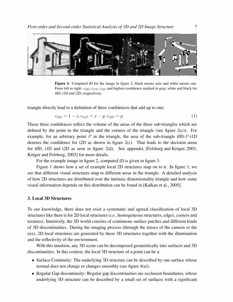
Figure 3. Computed iD for the image in figure 2, black means zero and white means one.From left to right: ci0D, ci1D, ci2D and highest confidence marked in gray, white and black fori0D, i1D and i2D, respectively.

triangle directly lead to a definition of three confidences that add up to one:

ci0D = 1− x, ci1D = x− y, ci2D = y. (1)

These three confidences reflect the volume of the areas of the three sub-triangles which aredefined by the point in the triangle and the corners of the triangle (see figure 2(c)). Forexample, for an arbitrary point P in the triangle, the area of the sub-triangle i0D-P -i1Ddenotes the confidence for i2D as shown in figure 2(c). That leads to the decision areasfor i0D, i1D and i2D as seen in figure 2(d). See appendix [Felsberg and Kruger, 2003,Kruger and Felsberg, 2003] for more details.

For the example image in figure 2, computed iD is given in figure 3.Figure 1 shows how a set of example local 2D structures map on to it. In figure 1, we

see that different visual structures map to different areas in the triangle. A detailed analysisof how 2D structures are distributed over the intrinsic dimensionality triangle and how somevisual information depends on this distribution can be found in [Kalkan et al., 2005].

3. Local 3D Structures

To our knowledge, there does not exist a systematic and agreed classification of local 3Dstructures like there is for 2D local structures (i.e., homogeneous structures, edges, corners andtextures). Intuitively, the 3D world consists of continuous surface patches and different kindsof 3D discontinuities. During the imaging process (through the lenses of the camera or theeye), 2D local structures are generated by these 3D structures together with the illuminationand the reflectivity of the environment.

With this intuition, any 3D scene can be decomposed geometrically into surfaces and 3Ddiscontinuities. In this context, the local 3D structure of a point can be a:

• Surface Continuity: The underlying 3D structure can be described by one surface whosenormal does not change or changes smoothly (see figure 4(a)).

• Regular Gap discontinuity: Regular gap discontinuities are occlusion boundaries, whoseunderlying 3D structure can be described by a small set of surfaces with a significant


d)

b)

c)

e)

a)

f)g)

h)

i)

j)

Figure 4. Illustration of the types of 3D discontinuities. (a) 2D image. (b) Continuity. (c)Orientation discontinuity. (d) Gap discontinuity. (e) Irregular gap discontinuity. (f)-(j) Therange images corresponding to (a)-(e). Note that the range images are scaled independentlyfor better visibility.


Figure 5. 10 of the 20 3D data sets used in the analysis. The points without range informationare marked in blue. The gray image shows the range data of the top-left scene. The horizontaland the vertical resolutions of the scenes respectively have the following ranges: [512-2048]and [390-2290]. The average resolution of the scenes is 1140x1001.

depth difference. The 2D and 3D views of an example gap discontinuity are shown infigure 4(d).

• Irregular Gap discontinuity: The underlying 3D structure shows high depth-variationthat can not be described by two or three surfaces. An example of an irregular gapdiscontinuity is shown in figure 4(e).

• Orientation Discontinuity: The underlying 3D structure can be described by two surfaceswith significantly different 3D orientations that meet at the center of the patch. This typeof discontinuity is produced by a change in 3D orientation rather than a gap betweensurfaces. An example for this type of discontinuity is shown in figure 4(c).

One interesting example is 3D corners of, for example, a cube. 3D corners would beclassified as regular gap discontinuities or orientation discontinuities, depending on the view.If the image patch includes parts of the background objects, then there is a gap discontinuity,and the 3D corner would be classified as a gap discontinuity. If, however, the camera centersthe corner so that all the adjacent edges of the cube are visible and no parts of other objectsare visible, then the 3D corner would be an orientation discontinuity.

3.1. Detection of Local 3D Structures

In this subsection, we define our measures for the three kinds of discontinuities that wedescribed above; namely, gap discontinuity, irregular gap discontinuity and orientationdiscontinuity. The measures for gap discontinuity, irregular gap discontinuity and orientationdiscontinuity of a patch P will be denoted by µGD(P ), µIGD(P ) and µOD(P ), respectively.The reader who is not interested in the technical details can jump directly to section 4.


3D discontinuities are detected in studies which involve range data processing, usingdifferent methods and under different names like two-dimensional discontinuous edge,jump edge or depth discontinuity for gap discontinuity; and, two-dimensional corner edge,crease edge or surface discontinuity for orientation discontinuity [Bolle and Vemuri, 1991,Hoover et al., 1996, Shirai, 1987].

In our analysis, we used chromatic range data of outdoor scenes which were obtainedfrom RIEGL UK Ltd. (http://www.riegl.co.uk/). There were 20 scenes in total, 10of which are shown in figure 5. The range of an object which does not reflect the laser beamback to the scanner or is out of the range of the scanner cannot be measured. These pointsare marked with blue in figure 5 and are not processed in our analysis. The horizontal andthe vertical resolutions of the scenes respectively have the following ranges: [512-2048] and[390-2290]. The average resolution of the scenes is 1140x1001.

3.1.1. Measure for Gap Discontinuity: µGD

Gap discontinuities can be measured or detected in a similar way than edges in 2D images;edge detection processes RGB-coded 2D images while for a gap discontinuity, one needs toprocess XYZ-coded 2D images ¶. In other words, gap discontinuities can be measured ordetected by taking the second order derivative of XYZ values [Shirai, 1987].

Measurement of a gap discontinuity is expected to operate on both the horizontal and thevertical axes of the 2D image; that is, it should be a two dimensional function. The alternativeis to discard the topology and do an ’edge-detection’ in sorted XYZ values, i.e., to operateas a one-dimensional function. Although we are not aware of a systematic comparison ofthe alternatives, for our analysis and for our data, the topology-discarding gap discontinuitymeasurement captured the underlying 3D structure better (of course, qualitatively, i.e., byvisual inspection). Therefore, we have adopted the topology-discarding gap discontinuitymeasurement in the rest of the paper.

For an image patch P of size N ×N , let,

X = ascending sort(Xi | i ∈ P),Y = ascending sort(Yi | i ∈ P), (2)

Z = ascending sort(Zi | i ∈ P),

and also, for i = 1, .., (N ×N − 2),

X∆ = | (Xi+2 −Xi+1)− (Xi+1 −Xi) | ,Y∆ = | (Yi+2 − Yi+1)− (Yi+1 − Yi) | , (3)

Z∆ = | (Zi+2 −Zi+1)− (Zi+1 −Zi) | ,

where Xi,Yi,Zi represents 3D coordinates of pixel i. Equation 3 takes the absolute value ofthe [+1, −2, +1] operator.

The sets X∆,Y∆ and Z∆ are the measurements of the jumps (i.e., second orderdifferentials) in the sets X ,Y and Z , respectively. A gap discontinuity can be defined simply

¶ Note that XYZ and RGB coordinate systems are not the same. However, detection of gap discontinuity inXYZ coordinates can be assumed to be a special case of edge detection in RGB coordinates.


Figure 6. Example histograms and the number of clusters that the function ψ(S) computes.ψ(S) finds one cluster in the left histogram and two clusters in the right histogram. Redline marks the threshold value of the function. X axis denotes the values for 3D orientationdifferences.

as a measure of these jumps in these sets. In other words:

µGD(P ) =h(X∆) + h(Y∆) + h(Z∆)

3, (4)

where the function h : S → [0, 1] over the set S measures the homogeneity of its argumentset (in terms of its ’peakiness’) and is defined as follows:

h(S) =1

#(S)×

∑i∈S

si

max(S), (5)

where #(S) is the number of the elements of S, and si is the ith element of the set S. Notethat as a homogeneous set (i.e., a non-gap discontinuity) S produces a high h(S) value, a gapdiscontinuity causes a low µGD value. Figure 8(c) shows the performance of µGD on one ofour scenes shown in figure 5.

It is known that derivatives like in equations 2 and 3 are sensitive to noise. Gaussian-based functions could be employed instead. In this paper, we chose simple derivatives fortheir faster computation times, and instead employed a more robust processing stage (i.e.,analyzing the uniformity of the distribution of derivatives) to make the measurement morerobust to noise. As shown in figure 8(c), this method can capture the underlying 3D structurewell.

3.1.2. Measure for Orientation Discontinuity: µOD

The orientation discontinuity of a patch P can be detected or measured by taking the 3Dorientation difference between the surfaces that meet in P . If the size of the patch P issmall enough, the surfaces can be, in practice, approximated by 2-pixel wide unit planes+.The histogram of the 3D orientation differences between every pair of unit planes forms onecluster for continuous surfaces and two clusters for orientation discontinuities.

For an image patch P of size N × N pixels, the orientation discontinuity measure is+ Note that using bigger planes have the disadvantage of losing accuracy in positioning which is very crucialfor the current analysis.


defined as:

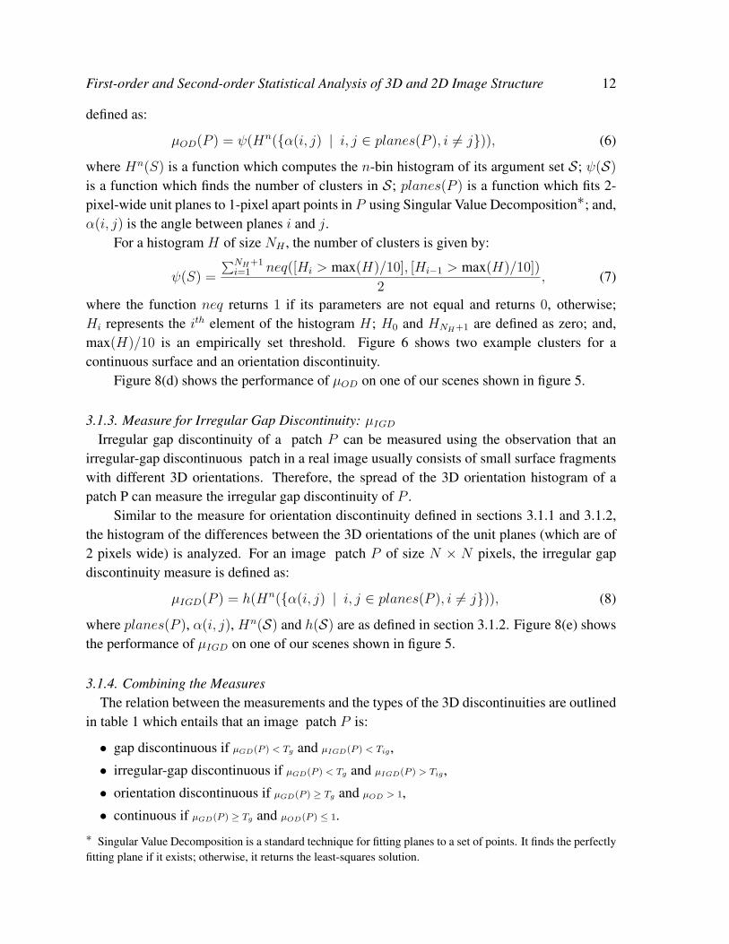
µOD(P ) = ψ(Hn(α(i, j) | i, j ∈ planes(P ), i 6= j)), (6)

where Hn(S) is a function which computes the n-bin histogram of its argument set S; ψ(S)

is a function which finds the number of clusters in S; planes(P ) is a function which fits 2-pixel-wide unit planes to 1-pixel apart points in P using Singular Value Decomposition∗; and,α(i, j) is the angle between planes i and j.

For a histogram H of size NH , the number of clusters is given by:

ψ(S) =

∑NH+1i=1 neq([Hi > max(H)/10], [Hi−1 > max(H)/10])

2, (7)

where the function neq returns 1 if its parameters are not equal and returns 0, otherwise;Hi represents the ith element of the histogram H; H0 and HNH+1 are defined as zero; and,max(H)/10 is an empirically set threshold. Figure 6 shows two example clusters for acontinuous surface and an orientation discontinuity.

Figure 8(d) shows the performance of µOD on one of our scenes shown in figure 5.

3.1.3. Measure for Irregular Gap Discontinuity: µIGD

Irregular gap discontinuity of a patch P can be measured using the observation that anirregular-gap discontinuous patch in a real image usually consists of small surface fragmentswith different 3D orientations. Therefore, the spread of the 3D orientation histogram of apatch P can measure the irregular gap discontinuity of P .

Similar to the measure for orientation discontinuity defined in sections 3.1.1 and 3.1.2,the histogram of the differences between the 3D orientations of the unit planes (which are of2 pixels wide) is analyzed. For an image patch P of size N × N pixels, the irregular gapdiscontinuity measure is defined as:

µIGD(P ) = h(Hn(α(i, j) | i, j ∈ planes(P ), i 6= j)), (8)

where planes(P ), α(i, j), Hn(S) and h(S) are as defined in section 3.1.2. Figure 8(e) showsthe performance of µIGD on one of our scenes shown in figure 5.

3.1.4. Combining the MeasuresThe relation between the measurements and the types of the 3D discontinuities are outlined

in table 1 which entails that an image patch P is:

• gap discontinuous if µGD(P ) < Tg and µIGD(P ) < Tig,

• irregular-gap discontinuous if µGD(P ) < Tg and µIGD(P ) > Tig,

• orientation discontinuous if µGD(P ) ≥ Tg and µOD > 1,

• continuous if µGD(P ) ≥ Tg and µOD(P ) ≤ 1.∗ Singular Value Decomposition is a standard technique for fitting planes to a set of points. It finds the perfectlyfitting plane if it exists; otherwise, it returns the least-squares solution.


c c c c c

cc c c c

0 32 64

0

32

640 32 64

0

32

640 32 64

0

32

640 32 64

0

32

640 32 64

0

32

64

0 32 64

0

32

640 32 64

0

32

640 32 64

0

32

640 32 64

0

32

640 32 64

0

32

64

b)

a)

c)

d)

d = 0 m d = 0.02 md = 0.01 m d = 0.03 m d = 0.04 m

a = 117 deg.a = 180 deg. a = 90 deg.a = 153 deg.a = 171 deg.

Figure 7. Results of the combined measures on artificial data. The camera and the rangescanner are denoted by c. (a) Gap discontinuity tests. There are two planes which are separatedby a distance d where d= 0, 0.01, 0.02, 0.03, 0.04 meters. (b) The detected discontinuities.Dark blue marks the boundary points where the measures are not applicable. Blue andorange respectively correspond to detected continuities and gap discontinuities. (c) Orientationdiscontinuity tests. There are two planes which are connected but separated with an angle awhere a=180, 171, 153, 117, 90 degrees. (d) The detected discontinuities. Dark blue marksthe boundary points where the measures are not applicable. Blue and green respectivelycorrespond to detected continuities and orientation discontinuities.

For our analysis, N , where NxN is the size of the patches, is set to 10 pixels. Bigger valuesfor N means larger support region for the measures, in which case different kinds of 3Ddiscontinuities might interfere in the patch. On the other hand, using smaller values wouldmake the measures very sensitive to noise. Other thresholds Tg and Tig are respectively setto 0.4 and 0.6. These values are empirically determined by testing the measures over a largeset of samples. Different values for these thresholds may result in wrong classifications oflocal 3D structures and may lead to different results than presented in this paper. Similarly,the number of bins, n, in Hn is empirically determined as 20.

Figure 7 shows the performance of the measures on two artificial scenes, one for gapdiscontinuity and one for orientation discontinuity for a set of depth and angle differencesbetween planes. In the figure, the detected discontinuity type is shown for each pixel. We seethat gap discontinuity can be detected reliable even if the gap difference is low. The sensitivityof the orientation discontinuity measure is around 160 degrees. However, the sensitivity of


a) b)

d)c) e)

Figure 8. The 3D and 2D information for one of the scenes shown in figure 5. Darkblue marks the points without range data. (a) 3D discontinuity. Blue: continuous surfaces,light blue: orientation discontinuities, orange: gap discontinuities and brown: irregular gapdiscontinuities. (b) Intrinsic Dimensionality. Homogeneous patches, edge-like and corner-like structures are encoded in colors brown, yellow and light blue, respectively. (c) Gapdiscontinuity measure µGD. (d) Orientation discontinuity measure µOD. (e) Irregular gapdiscontinuity measure µIGD.

Dis. Type µGD µIGD µOD

Continuity High value Don’t care 1

Gap Dis. Low value Low value Don’t careIrregular Gap Dis. Low value High value Don’t careOrientation Dis. High value Don’t care > 1

Table 1. The relation between the measurements and the types of the 3D discontinuities.

the measures would be different in real scenes due to the noise in the range data.For a real example scene from figure 5, the detected discontinuities are shown in figure

8(a). We see that the underlying 3D structure of the scene is reflected in figure 8(a).An interesting example is smoothly curved surfaces. Such a surface would not produce

jumps in equation 3 (since it is smooth), and therefore produce a high µGD value. Similarly,µOD would be 1 since there would be no peaks in the distribution of orientation differences. Inother words, a curved surface would be classified as a continuity by the measures introducedabove.

Note that this categorical combination of the measures appears to be against the


motivation that has been provided for the classification of local 2D structures where we hadadvocated a continuous approach. There are two reasons: (1) With continuous 3D measures,the dimensionality of the results would be four (origin variance, line variance, a 3D measureand the normalized frequency of the signals), which is difficult to visualize and analyze. Infact, the number of triangles that had to be shown in figure 9 would be 12, and it would bevery difficult to interpret all the triangles together. (2) It has been argued by several studies[Huang et al., 2000, Yang and Purves, 2003] that range images are much simpler and lesscomplex to analyze than 2D images. This suggests that it might be safer to have a categoricalclassification for range images.

4. First-order Statistics: Analysis of the Relation Between Local 3D and 2D Structure

In this section, we analyze the relation between local 2D structures and local 3D structure;namely, the likelihood of observing a 3D structure given the corresponding 2D structure (i.e.,P (3D Structure | 2D Structure)).

4.1. Results and Discussion

For each pixel of the scene (except where range data is not available), we computed the 3Ddiscontinuity type and the intrinsic dimensionality. Figures 8(a) and (b) show the imageswhere the 3D discontinuity and the intrinsic dimensionality of each pixel are marked withdifferent colors.

Having the 3D discontinuity type and the information about the local 2D structure ofeach point, we wanted to analyze what the likely underlying 3D structure is for a givenlocal 2D structure; that is, the conditional likelihood P (3D Discontinuity | 2D Structure).Using the available 3D discontinuity type and the information about the local 2D structure,other measurements or correlations between the range data and the image data could also becomputed in a further study.

P (3D Discontinuity | 2D Structure) is shown in figure 9. Note that the four triangles infigures 9(a), 9(b), 9(c) and 9(d) add up to one for all points of the triangle.

In figure 10, maximum likelihood estimates (MLE) of local 3D structures given local 2Dstructures are provided. Figure 10(a) shows the MLE from the distributions in figure 9. Dueto high likelihoods, gap discontinuities and continuities are the most likely estimates givenlocal 2D structures. Figure 10(b) shows the MLE from the normalized distributions: i.e., eachtriangle in figure 9 is normalized within itself so that its maximum likelihood is 1. This waywe can see the mostly likely local 2D structures for different local 3D structures.

• Figure 9(a) shows that homogeneous 2D structures are very likely to be formed by 3Dcontinuities as the likelihood P (Continuity | 2D Structure) is very high (bigger than 0.85)for the area where homogeneous 2D structures exist (marked with H in figure 9(a)). Thisobservation is confirmed in the MLE estimates of figure 10.Many surface reconstruction studies make use of a basic assumption that there is asmooth surface between any two points in the 3D world, if there is no contrast difference


0 0.5 10

0.5

1

0

0.1

0.2

0.3

0.4

0.5

0.6

0.7

0.8

0.9

1

0 0.5 10

0.5

1

0

0.1

0.2

0.3

0.4

0.5

0.6

0.7

0.8

0.9

1

0 0.5 10

0.5

1

0

0.05

0.1

0.15

0.2

0.25

0.3

0.35

0.4

0 0.5 10

0.5

1

0

0.01

0.02

0.03

0.04

0.05

0.06

0.07

0.08

0.09

0.1

Contrast Contrast

Ori

enta

tion

Var

ianc

e

Ori

enta

tion

Var

ianc

eO

rien

tatio

n V

aria

nce

Ori

enta

tion

Var

ianc

ea) Continuity b) Gap Discontinuity

c) Irregular Gap Discontinuity d) Orientation Discontinuity

Contrast Contrast

H

T

C

E H

T

C

E

H

T

C

EH

T

C

E

Figure 9. P (3D Discontinuity | 2D Structure). The schematic insets indi-cate the locations of the different types of 2D structures inside the triangle foreasy reference (the letters C, E, H, T represent corner-like, edge-like, homo-geneous and texture-like structures). (a) P (Continuity | 2D Structure). (b)P (Gap Discontinuity | 2D Structure). (c) P (Irregular Gap Discontinuity | 2D Structure). (d)P (Orientation Discontinuity | 2D Structure).

between these points in the image. This assumption has been first called as ’no news isgood news’ in [Grimson, 1983]. Figure 9(a) quantifies ’no news is good news’ and showsfor which structures and to what extent it holds: In addition to the fact that no news isin fact good news, figure 9(a) shows that news, especially texture-like structures andedge-like structures, can also be good news (see below). Homogeneous 2D structurescannot be used for depth extraction by correspondence-based methods, and only weakor no information from these structures is processed by the cortex. Unfortunately, thevast majority of local image structure is of this type (see, e.g., [Kalkan et al., 2005]).On the other hand, homogeneous structures indicate ’no change’ in depth which is theunderlying assumption of interpolation algorithms.


(a) (b)

Figure 10. Maximum likelihood estimates of local 3D structures given local 2D structures.Numbers 1, 2, 3 and 4 represent continuity, gap discontinuity, orientation discontinuity andirregular gap discontinuity, respectively. (a) Raw maximum likelihood estimates. Note thatthe estimates are dominated by continuities and gap discontinuities. (b) Maximum likelihoodestimates from normalized likelihood distributions: the triangles provided in figure 9 arenormalized within themselves so that the maximum likelihood of P (X | 2D Structure) is 1 forX being continuity, gap discontinuity, irregular gap discontinuity and orientation discontinuity.

• Edges are considered as important sources of information for object recognition andreliable correspondence finding. Approximately 10% of local 2D structures are of thattype (see, e.g., [Kalkan et al., 2005]). Figures 9(a), (b) and (d) together with the MLEestimates in figure 10 show that most of the edges are very likely to be formed bycontinuous surfaces or gap discontinuities. Looking at the decision areas for differentlocal 2D structures shown in figure 2(d), we see that the edges formed by continuoussurfaces are mostly low-contrast edges (figure 9(a)); i.e., the origin variance is close to0.5. Little percentage of the edges are formed by orientation discontinuities (figure 9(d)).

• Figures 9(a) and (b) show that well-defined corner-like structures are formed by eithergap discontinuities or continuities.

• Figures 9(d) and 10 show that textures also are very likely to be formed by surfacecontinuities and irregular gap discontinuities.Finding correspondences becomes more difficult with the lack or repetitiveness ofthe local structure. The estimates of the correspondences at texture-like structuresare naturally less reliable. In this sense, the likelihood that certain textures areformed by continuous surfaces (shown in figure 9(a)) can be used to model stereomatching functions that include interpolation as well as information about possiblecorrespondences based on the local image information.It is remarkable that local 2D structures mapping to different sub-regions in the triangle

are formed by rather different 3D structures. This clearly indicates that these different 2Dstructures should be used in different ways for surface reconstruction.


(a) (b) (c)

Figure 11. Illustration of the relation between the depth of homogeneous 2D structures andthe bounding edges. (a) In the case of the cube, the depth of homogeneous image area andthe bounding edges are related. However, in the case of round surfaces, (b) the depth ofhomogeneous 2D structures may not be related to the depth of the bounding edges. (c) In thecase of a cylinder, we see both cases of the relation as illustrated in (a) and (b).

5. Second-Order Statistics: Analysis of Co-planarity between 3D Edges andContinuous Patches

As already mentioned in section 1, it is not possible to extract depth at homogeneous 2Dstructures (in the rest of the paper, a homogeneous 2D structure that corresponds to a 3Dcontinuity will be called a mono) using methods that make use of multiple views for 3Dreconstruction. In this section, by making use of the ground truth range data, we investigateco-planarity relations between the depth at homogeneous 2D structures and the edges thatbound them. This relation is illustrated for a few examples in figure 11.

For the analysis, we used the chromatic range data set that we also used for the first-orderanalysis in section 4. Samples from the dataset are displayed in figure 5.

In the following subsection, we explain how we analyze the relation. The results arepresented and discussed in section 5.2.

5.1. Methods

This subsection provides the procedural details of how the analysis is performed.The analysis is performed in three stages: First, local 2D and 3D representations of the

scene are extracted from the chromatic range data. Second, a data set is constructed out ofeach pair of edge features, associating the monos that are likely to be coplanar to those edgesto them (see section 5.1.2 for what we mean by relevance). Third, the coplanarity between themonos and the edge features that they are associated to are investigated. An overview of theanalysis process is sketched in figure 12, which roughly lists the steps involved.

5.1.1. RepresentationUsing the 2D image and the associated 3D range data, a representation of the scene is

created in terms of local compository 2D and 3D features denoted by π. In this process,first, 2D features are extracted from the image information, and at the locations of these 2Dfeatures, 3D features are computed. The complementary information from the 2D and 3D


Investigate the coplanarity

edges and the monosrelations between pairs of

Analysis

Representation

Data Collection

Representation

RepresentationLocal 2D

Local 3D

3DDiscontinuity

Go over everyproximate pair of

edge features

Associate the"interesting" monos

to each pair

Figure 12. Overview of the analysis process. First, local 2D and 3D representations of thescene are extracted from the chromatic range data. Second, a data set is constructed out of eachpair of edge features, associating the monos that are likely to be coplanar (i.e., ”interesting”)to them (see section 5.1.2 for what we mean by relevance). Third, the coplanarity between themonos and the edge features that they are associated to are investigated.

features are then merged at each valid position, where validity is only defined by havingenough range data to extract a 3D representation.

For homogeneous and edge-like structures, different representations are needed due todifferent underlying structures. For this reason, we have two different definitions of π denotedrespectively by πe (for edge-like structures) and πm (for monos) and formulated as:

πm = (X3D,X2D, c,p), (9)

πe = (X3D,X2D, φ2D, c1, c2,p1,p2), (10)

where X3D and X2D denote 3D and 2D positions of the 3D entity; φ2D is the 2D orientationof the 3D entity; c1 and c2 are the 2D color representation of the surfaces of the 3D entity; c

represents the color of πm; p1 and p2 are the planes that represent the surfaces that meet atthe 3D entity; and p represents the plane of πm (see figure 13). Note that πm does not haveany 2D orientation information (because it is undefined for homogeneous structures), and πe

has two color and plane representations to the ’left’ and ’right’ of the edge.The process of creating the representation of a scene is illustrated in figure 13.In our analysis, the entities are regularly sampled from the 2D information. The sampling

size is 10 pixels. See [Kruger et al., 2003, Kruger and Worgotter, 2005] for details.Extraction of the planar representation requires knowledge about the type of local 3D

structure of the 3D entity (see figure 13). Namely, if the 3D entity is a continuous surface,then only one plane needs to be extracted; if the 3D entity is an orientation discontinuity, thenthere will be two planes for extraction; if the 3D entity is a gap discontinuity, then there willalso be two planes for extraction.

In the case of a continuous surface, a single plane is fitted to the set of 3D points inthe 3D entity in question. For orientation discontinuous 3D structures, extraction of theplanar representation is not straight-forward. For these structures, our approach was to fit


2D image Range image Discont. image

Local 2D Representation Local 3D Representation

OROR

c1, c2

φ2D

c

p

p1,p2

πm = (X3D,X2D, c,p)

πe = (X3D,X2D, φ2D, c1, c2,p1,p2)

Figure 13. Illustration of the representation of a 3D entity. From the 2D and 3D information,local 2D and 3D representation is extracted.

unit-planes− to the 3D points of the 3D entity and find the two clusters in these planes usingk-means clustering of the 3D orientations of the small planes. Then, one plane is fitted foreach of the two clusters, producing the bi-fold planar representation of the 3D entity.

Color representation is extracted in a similar way. If the image patch is a homogeneousstructure, then the average color of the pixels in the patch is taken to be the colorrepresentation. If the image patch is edge-like, then it has two colors separated by the linewhich goes through the center of the image patch and which has the 2D orientation of theimage patch. In this case, the averages of the colors of the different sides of the edge definethe color representation in terms of c1 and c2. If the image patch is corner-like, the colorrepresentation becomes undefined.

5.1.2. Collecting the Data SetIn our analysis, we form pairs out of πes that are close enough (see below), and for each

pair, we check whether monos in the scene are coplanar to the elements of the pair or not.As there are plenty of monos in the scene, we only consider a subset of monos for each pairof πe that we suspect to be relevant to the analysis because otherwise, the analysis becomescomputationally intractable. The situation is illustrated in figure 14(a). In this figure, two πe

and three regions are shown; however, only one of these regions (i.e., region A) is likely tohave coplanar monos (e.g., see figure 11(a)). This assumption is based on the observation of− By unit-planes, we mean planes that are fitted to the 3D points that are 1-pixel apart in the 2D image.


50px

10px

Region A

Intersection Point (IP)

Region B

Region C

a)

e)

b)

c)

d)

100px

Intersection Point (IP)

πe

1

πe

2

(X2D)′2

f2 = (X2D)1

f1 = (X2D)′1

(X2D)2πe

2

πe

1

Figure 14. (a) Given a pair of edge features, coplanarity relation can be investigated forhomogeneous image patches inside regions A, B and C. However, due to computationalintractability reasons, this paper is concerned in making the analysis only in region A (seethe text for more details). (b)-(d) A few different configurations of edge features that mightbe encountered in the analysis. The difficult part of the investigation is to make thesedifferent configurations comparable, which can be achieved by fitting a shape (like square,rectangle, circle, parallelogram, ellipse) to these configurations. (e) The ellipse, among thealternative shapes (i.e., square, rectangle, circle, parallelogram) turns out to describe thedifferent configurations shown in (b)-(d) better. For this reason, ellipse is for analyzingcoplanarity relations in the rest of the paper. See the text for details on how the parameters ofthe ellipse are set.

how objects are formed in the real world: objects have boundaries which consists of edge-likestructures who bound surfaces, or image areas, of the object. The image area that is boundedby a pair of edge-like structures is likely to be the area that has the normals of both structures.For convex surfaces of the objects, the area that is bounded belongs to the object; however, inthe case of concave surfaces, the area covered may also be from other objects, and the extentof the effect of this is part of the analysis.

Let P denote the set of pairs of proximate πes whose normals intersect. P can be defined


as:

P =(πe

1, πe2) | ∀πe

1, πe2, π

e1 ∈ Ω(πe

2), I(⊥ (πe1),⊥ (πe

2)), (11)

where Ω(πe) is the N-pixel-2D-neighborhood of πeo; ⊥ (πe) is the 2D line orthogonal to the2D orientation of πe, i.e., the normal of πe; and, I(l1, l2) is true if the lines l1 and l2 intersect.We have taken N to be 100.

It turns out that there are a lot of different configurations possible for a pair of edgefeatures based on relative position and orientation, which are illustrated for a few cases infigure 14(b)-(d). The difficult part of the investigation is to be able to compare these differentconfigurations. One way to achieve this is to fit a shape to region A which can normalize thecoplanarity relations by its size in order to make them comparable (see section 5.2 for moreinformation).

The possible shapes would be square, rectangle, parallelogram, circle and ellipse.Among the alternatives, it turns out that an ellipse (1) is computationally cheap and (2) fits todifferent configurations of π1 and π2 under different orientations and distances without leavingregion A much. Figure 14(e) demonstrates the ellipse generated by an example pair of edgesin figure 14(a). The center of the ellipse is at the intersection of the normals of the edges,which we call the intersection point (IP) in the rest of the paper.

The parameters of an ellipse are composed of two focus points f1, f2 and the minor axisb. In our analysis, the more distant 3D edge determines the foci of the ellipse (and, hence,the major axis), and the other 3D edge determines the length of the minor axis. Alternatively,the ellipse can be constructed by minimizing an energy functional which optimizes the areaof the ellipse inside region A and going through the features π1 and π2. However, for the sakeof speed issues, the ellipse is constructed without optimization.

See appendix A.1 for details on how we determine the parameters of the ellipse.For each pair of edges in P , the region to analyze coplanarity is determined by

intersecting the normals of the edges. Then, the monos inside the ellipse are associated tothe pair of edges.

Note that a πe has two planes that represent the underlying 3D structure. When πesbecome associated to monos, only one plane, the one that points into the ellipse, remainsrelevant. Let πse denote the semi-representation of πe which can be defined as:

πse = (X3D,X2D, c,p). (12)

Note that πse is equivalent to the definition of πm in equation 10.Let T denote the data set which stores P and the associated monos which can be

formulated as:

T = (πse1 , π

se2 , π

m) | (πe1, π

e2) ∈ P , πm ∈ Sm, πm ∈ E(πe

1, πe2), (13)

where Sm is the set of all πm.A pair of πes and the set of monos associated to them are illustrated in figure 15. The

figure shows the edges and the monos (together with ellipse) in 2D and 3D.

o In other words, the Euclidean image distance between the structures should be less than N.


(a) (b)

(c) (d)

Figure 15. Illustration of a pair of πe and the set of monos associated to them. (a) The inputscene. A pair of edges (marked in blue) and the associated monos (marked in green) with anellipse (drawn in black) around them shown on the input image. See (c) for a zoomed version.(b) The 3D representation of the scene in our 3D visualization software. This representationis created from the range data corresponding to (a) and is explained in the text. (c) The partof the input image from (a) where the edges, the monos and the ellipse are better visible. (d)A part of the 3D representation (from (b)) corresponding to the pair of edges and the monosin (c) is displayed in detail where the edges are shown with blue margins; the monos with theedges are shown in green (all monos are coplanar with the edges). The 3D entities are drawnin rectangles because of the high computational complexity for drawing circles.

5.1.3. Definition of coplanarityTwo entities are coplanar if they are on the same plane. Coplanarity of edge features and

monos is equivalent to coplanarity of two planar patches: two planar patches A and B arecoplanar if (1) they are parallel and (2) the planar distance between them is zero.

See appendix A.2 for more information.

5.2. Results and Discussions

The data set T defined in equation 13 consists of pairs of πe1, πe

2 and the associated monos.Using this set, we compute the likelihood that a mono is coplanar with πe

1and/or πe2 against a

distance measure.The results of our analysis are shown in figures 16 and 18 and 19.In figure 16(b), the likelihood of the coplanarity of a mono against the distance to πe

1 orπe

2 is shown. This likelihood can be denoted formally as P (cop(πm, πe1 & πe

2) | dN(πm, πe))

where cop(πm, πe1 & πe

2) is defined as cop(πe1, π

e2) ∧ cop(πm, πe), and πe is either πe

1 or πe2.


0 0.25 0.5 0.75 10

0.1

0.2

0.3

0.4

0.5

0.6

0.7

0.8

0.9

1P( cop(πm, πe) | d(πm, πe))

dN

(πm, πe)

0 0.25 0.5 0.75 10

0.5

1

1.5

2

2.5

3

3.5x 10

5 # of πm

dN

(πm, πe)

(a)

0 0.25 0.5 0.75 10

0.1

0.2

0.3

0.4

0.5

0.6

0.7

0.8

0.9

1

P( cop(πm, πe1 & πe

2) | d(πm, πe))

dN

(πm, πe)

0 0.25 0.5 0.75 10

0.5

1

1.5

2

2.5

3

3.5x 10

5 # of πm

dN

(πm, πe)

(b)

Figure 16. Likelihood distribution of coplanarity of monos. In each sub-figure, left-plotshows the likelihood distribution whereas right-plot shows the frequency distribution. (a) Thelikelihood of the coplanarity of a mono with πe

1 or πe2 against the distance to πe

1 or πe2. This is

the unconstrained case; i.e., the case where there is no information about the coplanarity of πe1

and πe2. (b) The likelihood of the coplanarity of a mono with πe

1 and πe2 against the distance to

πe1 or πe

2.

0 0.25 0.5 0.75 1 0

0.2

0.4

0.6

0.8

1P(cop(πm, πe) | d(πm, πe)

dN

(πm, πe)

(a)

0 0.25 0.5 0.75 1 0

0.2

0.4

0.6

0.8

1

P(cop(πm, πe1&πe

2) | d(πm, πe)

dN

(πm, πe)

(b)

Figure 17. Likelihoods from figures 16(a) and 16(b) with a more strict coplanarity relation(namely, we set the thresholds Tp and Td to 10 degrees and 0.2, respectively. See Appendixfor more information about these thresholds). (a) Figure 16(a) with more strict coplanarityrelation. (b) Figure 16(b) with more strict coplanarity relation.

The normalized distance measure] dN(πm, πe) is defined as:

dN(πm, πe) =d(πm, πe)

2√d(πe

1, IP )2 + d(πe2, IP )2

, (14)

] In the following plots, the distance means the Euclidean distance in the image domain.


0 0.125 0.25 0.375 0.50

0.1

0.2

0.3

0.4

0.5

0.6

0.7

0.8

P( cop(πm, πe1&πe

2) | d(πm, IP))

dN

(πm, IP)

0 0.125 0.25 0.375 0.50

2

4

6

8

10x 10

4 # of πm

dN

(πm, IP)

Figure 18. The likelihood of the coplanarity of a mono against the distance to IP . Left-plotshows the likelihood distribution whereas right-plot shows the frequency distribution.

0 0.25 0.5 0.75 10

0.25

0.5

0.75

1

P( cop(πm, πe1 & πe

2) | d

N(πm, πe

1), d

N(πm, πe

2))

dN

(πm, πe1)

d N(π

m, π

e 2)

0

0.2

0.4

0.6

0.8

0 0.25 0.5 0.75 10

0.25

0.5

0.75

1# of πm

dN

(πm, πe1)

d N(π

m, π

e 2)

0

500

1000

1500

2000

2500

3000

3500

Figure 19. The likelihood of the coplanarity of a mono against the distance to πe1 and πe

2. Left-plot shows the likelihood distribution whereas right-plot shows the frequency distribution.

where πe is either πe1 or πe

2, and IP is the intersection point of πe1 and πe

2. We see in figure16(b) that the likelihood decreases when a mono is more distant from an edge. However,when the distance measure gets closer to one, the likelihood increases again. This is because,when a mono gets away from either πe

1 or πe2, it gets closer to the other πe.

In figure 16(a), we see the unconstrained case of figure 16(b); i.e., the case wherethere is no information about the coplanarity of πe

1 and πe2; namely, the likelihood

P (cop(πm, πe) | dN(πm, πe)) where πe is either πe1 or πe

2. The comparison with figure 16(b)shows that the existence of another edge in the neighborhood increases the likelihood offinding coplanar structures. As there is no other coplanar edge in the neighborhood, thelikelihood does not increase when the distance is close to one (compare with figure 16(b)).

It is intuitive to expect symmetries in figure 16. However, as (1) the roles of πe1 and πe

2

in the ellipse are fixed, and (2) one πe is guaranteed to be on the major axis, and the other πe

may or may not be on the minor axis, the symmetry is not observable in figure 16.To see the effect of the coplanarity relation on the results, we reproduced figures 16(a)

and 16(b) with a more strict coplanarity relation (namely, we set the thresholds Tp and Td to


10 degrees and 0.2, respectively. See Appendix for more information about these thresholds).The results with more constrained coplanarity relation are shown in figure 17. Although thelikelihood changes quantitatively, the figure shows the qualitative behaviours that have beenobserved with the standard thresholds. Moreover, we cross-checked the results for subsets ofthe original dataset (results not provided here) and confirmed the same qualitative results.

In figure 18, the likelihood of the coplanarity of a mono against the distance to IP (i.e.,P (cop(πm, πe

1 & πe2) | dN(πm, IP ))) is shown. We see in the figure that the likelihood shows

a flat distribution against the distance to IP.In figure 19, the likelihood of the coplanarity of a mono against the distance to πe

1 and πe2

(i.e., P (cop(πm, πe1 & πe

2) | dN(πm, πe1), dN(πm, πe

2))) is shown. We see that when πm is closeto πe

1 or πe2, it is more likely to be coplanar with πe

1 and πe2 than when it is equidistant to both

edges. The reason is that, when πm moves away from an equidistant point, it becomes closerto the other edge, in which case the likelihood increases as shown in figure 16(b).

The results, especially figures 16(b) and 16(a) confirm the importance of the relationillustrated in figure 11(a).

6. Discussion

6.1. Summary of the findings

Section 4.1 analyzed the likelihood P (3D Structure | 2D Structure). In this section, weconfirm and quantify the assumptions used in several surface interpolation studies. Our mainfindings from this section are as follows:

• As expected, homogeneous 2D structures are formed by continuous surfaces.

• Surprisingly, considerable amount of edges and texture-like structures are likely to beformed by continuous surfaces too. However, we confirm the expectation that gapdiscontinuities and orientation discontinuities are likely to be the underlying 3D structurefor edge-like structures. As for texture-like structures, they may also be formed byirregular gap discontinuities.

• Corner-like structures, on the other hand, are mainly formed by gap discontinuities.

In section 5.2, we investigated the predictability of depth at homogeneous 2D structures.We confirm the basic assumption that closer entities are very likely to be coplanar. Moreover,we provide results showing that this likelihood increases if there are more edge features in theneighborhood.

6.2. Interpretation of the findings

Existing psychophysical experiments (see, e.g., [Anderson et al., 2002, Collett, 1985]), com-putational theories (see, e.g., [Barrow and Tenenbaum, 1981, Grimson, 1982, Terzopoulos, 1988])and the observation that humans can perceive depth at weakly textured areas suggest that inthe human visual system, an interpolation process is realized that, starting with the local


analysis of edges, corners and textures, computes depth also in areas where correspondencescannot easily be found.

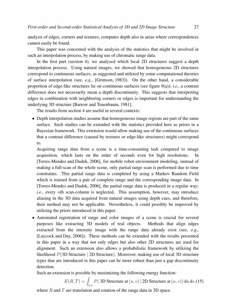
This paper was concerned with the analysis of the statistics that might be involved insuch an interpolation process, by making use of chromatic range data.

In the first part (section 4), we analyzed which local 2D structures suggest a depthinterpolation process. Using natural images, we showed that homogeneous 2D structurescorrespond to continuous surfaces, as suggested and utilized by some computational theoriesof surface interpolation (see, e.g., [Grimson, 1983]). On the other hand, a considerableproportion of edge-like structures lie on continuous surfaces (see figure 9(a)); i.e., a contrastdifference does not necessarily mean a depth discontinuity. This suggests that interpretingedges in combination with neighboring corners or edges is important for understanding theunderlying 3D structure [Barrow and Tenenbaum, 1981].

The results from section 4 are useful in several contexts:

• Depth interpolation studies assume that homogeneous image regions are part of the samesurface. Such studies can be extended with the statistics provided here as priors in aBayesian framework. This extension would allow making use of the continuous surfacesthat a contrast difference (caused by textures or edge-like structures) might correspondto.Acquiring range data from a scene is a time-consuming task compared to imageacquisition, which lasts on the order of seconds even for high resolutions. In[Torres-Mendez and Dudek, 2006], for mobile robot environment modeling, instead ofmaking a full-scan of the whole scene, only partial range scan is performed due to timeconstraints. This partial range data is completed by using a Markov Random Fieldwhich is trained from a pair of complete range and the corresponding image data. In[Torres-Mendez and Dudek, 2006], the partial range data is produced in a regular way;i.e., every nth scan-column is neglected. This assumption, however, may introducealiasing in the 3D data acquired from natural images using depth cues, and therefore,their method may not be applicable. Nevertheless, it could possibly be improved byutilizing the priors introduced in this paper.

• Automated registration of range and color images of a scene is crucial for severalpurposes like extracting 3D models of real objects. Methods that align edgesextracted from the intensity image with the range data already exist (see, e.g.,[Laycock and Day, 2006]). These methods can be extended with the results presentedin this paper in a way that not only edges but also other 2D structures are used foralignment. Such an extension also allows a probabilistic framework by utilizing thelikelihood P (3D Structure | 2D Structure). Moreover, making use of local 3D structuretypes that are introduced in this paper can be more robust than just a gap discontinuitydetection.Such an extension is possible by maximizing the following energy function:

E(R, T ) =∫

u,vP ( 3D Structure at (u, v) | 2D Structure at (u, v)) du dv,(15)

where R and T are translation and rotation of the range data in 3D space.


In the second part (section 5), we analyzed whether depth at homogeneous 2D structuresis related to the depth of edge-like structures in the neighborhood. Such an analysis isimportant for understanding the possible mechanisms that could underlie depth interpolationprocesses. Our findings show that an edge feature provides significant evidence for makingdepth prediction at a homogeneous image patch that is in the neighborhood. Moreover, theexistence of a second edge feature in its neighborhood which is not collinear with the firstedge feature increases the likelihood of the prediction.

Using second order relations and higher order features for representing the 2D image and3D range data, we produce confirming results that the range images are simpler to analyzecompared to 2D images (see, [Huang et al., 2000, Yang and Purves, 2003]).

By extracting a more complex representation than existing range-data analysis studies,we could point to the intrinsic properties of the 3D world and its relation to the image data.This analysis is important because (1) it may be that the human visual system is adaptedto the statistics of the environment [Brunswik and Kamiya, 1953, Knill and Richards, 1996,Krueger, 1998, Olshausen and Field, 1996, Purves and Lotto, 2002, Rao et al., 2002], and (2)it may be used in several computer vision applications (for example, depth estimation)in a similar way as in [Elder and Goldberg, 2002, Elder et al., 2003, Pugeault et al., 2004,Zhu, 1999].

In our current work, the likelihood distributions are being used for estimating the 3Ddepth at homogeneous 2D structures from the depth of bounding edge-like structures.

6.3. Limitations of the current work

The first limitation is due to the type of scenes that have been used; i.e., scenes of man-madeenvironments which also included trees. Alternative scenes could include pure forest scenesor scenes taken from an environment with totally round objects. However, we believe that ourdataset captures the general properties of the scenes that a human being encounters in dailylife.

Different scenes might produce quantitatively different but qualitatively similar results.For example, forest scenes would produce much more irregular gap discontinuities than thecurrent scenes; however, our conclusions regarding the link between textures and irregular gapdiscontinuities would still hold. Moreover, coplanarity relations would be harder to predict forsuch scenes since (depending on the scale) surface continuities are harder to find; however, ona bigger scale, some forest scenes are likely to produce the same qualitative results presentedin this paper because of piecewise planar leaves which are separated by gap discontinuities.

It should be noted that acquisition of range data with color images is very hard for forestscenes since the color image of the scene is taken after the scene is scanned with the scanner.During this period, the leaves and the trees may move (due to wind etc.), making the rangeand the color data inconsistent. In office environments, a similar problem arises: due to lateralseparation between the digital camera and range scanner, there is the parallax problem, whichagain produces inconsistent range-color association. For an office environment, a small-scalerange scanner needs to be used.


The statistics presented in this paper can be extended by analyzing forest scenes, officescenes etc. independently. The comparison of such independent analyses should provide moreinsights into the relations that this paper have investigated but we believe that the qualitativeconclusions of this paper would still hold.

It would be interesting to see the results presented in the paper by changing the measurefor surface continuity so that it can separate planar and curved surfaces. We believe that sucha change would effect only the second part of the paper.

7. Acknowledgements

We would like to thank RIEGL UK Ltd. for providing us with 3D range data, andNicolas Pugeault for his comments on the text. This work is supported by the European-funded DRIVSCO project, and an extension of two conference publications of the authors:[Kalkan et al., 2006, Kalkan et al., 2007].

Appendix

A.1. Parameters of an ellipse

Let us denote the position of two 3D edges πe1, π

e2 by (X2D)1 and (X2D)2 respectively. The

vectors between the 3D edges and IP (let us call l1 and l2) can be defined as:

l1 = ((X2D)1 − IP ),

l2 = ((X2D)2 − IP ). (16)

Having defined l1 and l2, the ellipse E(πe1, π

e2) is as follows:

E(πe1, π

e2) =

f1 = (X2D)1, f2 = (X2D)′1, b = |l2| if |l1| > |l2|,f1 = (X2D)2, f2 = (X2D)′2, b = |l1| otherwise.

(17)

where (X2D)′ is symmetrical with X2D around the intersection point and on the line definedby X2D and IP (as shown in figure 14(e)).

A.2. Definition of coplanarity

Let πs denote either a semi-edge πse or a mono πm. Two πs are coplanar iff they are on thesame plane. When it comes to measuring coplanarity, two criteria need to be tested:

(i) Angular criterion: For two πs to be coplanar, the angular difference between theorientation of the planes that represent them should be less than a threshold. A situationis illustrated in figure 20(a) where angular criterion holds but the planes are not coplanar.

(ii) Distance-based criterion: For two πs to be coplanar, the distance between the center ofthe first πs and the plane defined by the other πs should be less than a threshold. Infigure 20(b), B and C are at the same distance to the plane P which is the plane definedby the planar patch A. However, C is more distant to the center of A than B, and in thispaper, we treat that C is more coplanar to A than B is to A. The reason for this can be


B

A

(a)

d

A

B

C

P

d

(b)

Figure 20. Criteria for coplanarity of two planes. (a) According to the angular-differencecriterion of coplanarity, entities A and B will be measured as coplanar although they are ondifferent planes. In (b), P is the plane defined by entity A. According to the distance-basedcoplanarity definition, entities B and C have the same measure of coplanarity. However, entityC which is more distant to entity A should have a higher measure of coplanarity than entity Balthough they have the same distance to plane P (see the text).

clarified with an example: Assume that A, B and C are all parallel, and that the planarand the Euclidean distances between A and B are both D units, and between A and C arerespectively D and n × D. It is straightforward to see that although B and C have thesame planar distances to A, for n >> 1, C should have a higher coplanarity measure.

It is sufficient to combine these two criteria as follows:

cop(πs1, π

s2) = α(pπs

1 , pπs2) < Tp AND

d(pπs1 , πs

2)/d(πs1, π

s2) < Td, (18)

where pπs is the plane associated to πs; α(p1,p2) is the angle between the orientations of p1

and p2; and, d(., .) is the Euclidean distance between two entities.In our analysis, we have empirically chosen Tp and Td as 20 degrees and 0.5, respectively.

Again, like the parameters set in section 3.1.4, these values are determined by testing thecoplanarity measure over different samples. Tp is the limit for angular separation betweentwo planar patches. Bigger values would relax the coplanarity measure, and vice versa. Td

restricts the distances between the patches; in analogy to Tp, Td can be used to relax thecoplanarity measure. As shown in figure 17 for a stricter coplanarity definition (with Tp andTd set to 10 degrees and 0.2), different values for these thresholds would quantitatively butnot qualitatively change the results presented in section 5.

References

[Anderson et al., 2002] Anderson, B. L., Singh, M., and Fleming, R. W. (March 2002). The interpolation ofobject and surface structure. Cognitive Psychology, 44:148–190(43).

[Barrow and Tenenbaum, 1981] Barrow, H. G. and Tenenbaum, J. M. (1981). Interpreting line drawings asthree-dimensional surfaces. Artificial Intelligence, 17:75–116.

[Bolle and Vemuri, 1991] Bolle, R. M. and Vemuri, B. C. (1991). On three-dimensional surface reconstructionmethods. IEEE Transactions on Pattern Analysis and Machine Intelligence, 13(1):1–13.


[Bruce et al., 2003] Bruce, V., Green, P. R., and Georgeson, M. A. (2003). Visual Perception: Physiology,Psychology and Ecology. Psychology Press, 4th edition.

[Brunswik and Kamiya, 1953] Brunswik, E. and Kamiya, J. (1953). Ecological cue–validity of ’proximity’ andof other Gestalt factors. American Journal of Psychologie, LXVI:20–32.

[Collett, 1985] Collett, T. S. (1985). Extrapolating and Interpolating Surfaces in Depth. Royal Society ofLondon Proceedings Series B, 224:43–56.

[Coxeter, 1969] Coxeter, H. (1969). Introduction to Geometry (2nd ed.). Wiley & Sons.[Elder and Goldberg, 2002] Elder, H. and Goldberg, R. (2002). Ecological statistics of gestalt laws for the

perceptual organization of contours. Journal of Vision, 2(4):324–353.[Elder et al., 2003] Elder, J. H., Krupnik, A., and Johnston, L. A. (2003). Contour grouping with prior models.

IEEE Transactions on Pattern Analysis and Machine Intelligence, 25(25):1–14.[Felsberg and Kruger, 2003] Felsberg, M. and Kruger, N. (2003). A probablistic definition of intrinsic

dimensionality for images. Pattern Recognition, 24th DAGM Symposium.[Field et al., 1993] Field, D. J., Hayes, A., and Hess, R. F. (1993). Contour integration by the human visual

system: evidence for a local ”association field”. Vision Research, 33(2):173–193.[Gallant et al., 1994] Gallant, J. L., Essen, D. C. V., and Nothdurft, H. C. (1994). Early Vision and Beyond,

chapter : Two-dimensional and three-dimensional texture processing in visual cortex of the macaquemonkey, pages 89–98. MA: MIT Press.

[Grimson, 1982] Grimson, W. E. L. (1982). A Computational Theory of Visual Surface Interpolation. RoyalSociety of London Philosophical Transactions Series B, 298:395–427.

[Grimson, 1983] Grimson, W. E. L. (1983). Surface consistency constraints in vision. Computer Vision,Graphics and Image Processing, 24(1):28–51.

[Guzman, 1968] Guzman, A. (1968). Decomposition of a visual scene into three-dimensional bodies. AFIPSFall Joint Conference Proceedings, 33:291–304.

[Hoover et al., 1996] Hoover, A., Jean-Baptiste, G., Jiang, X., Flynn, P. J., Bunke, H., Goldgof, D. B., Bowyer,K., Eggert, D. W., Fitzgibbon, A., and Fisher, R. B. (1996). An experimental comparison of range imagesegmentation algorithms. IEEE Transactions on Pattern Analysis and Machine Intelligence, 18(7):673–689.

[Howe and Purves, 2002] Howe, C. Q. and Purves, D. (2002). Range image statistics can explain the anomalousperception of length. PNAS, 99(20):13184–13188.

[Howe and Purves, 2004] Howe, C. Q. and Purves, D. (2004). Size contrast and assimilation explained by thestatistics of natural scene geometry. Journal of Cognitive Neuroscience, 16(1):90–102.

[Huang et al., 2000] Huang, J., Lee, A. B., and Mumford, D. (2000). Statistics of range images. CVPR,1(1):1324–1331.

[Hubel and Wiesel, 1969] Hubel, D. and Wiesel, T. (1969). Anatomical demonstration of columns in themonkey striate cortex. Nature, 221:747–750.

[Kalkan et al., 2005] Kalkan, S., Calow, D., Worgotter, F., Lappe, M., and Kruger, N. (2005). Local imagestructures and optic flow estimation. Network: Computation in Neural Systems, 16(4):341–356.

[Kalkan et al., 2006] Kalkan, S., Worgotter, F., and Kruger, N. (2006). Statistical analysis of local 3d structurein 2d images. CVPR, 1:1114–1121.

[Kalkan et al., 2007] Kalkan, S., Worgotter, F., and Kruger, N. (2007). Statistical analysis of second-orderrelations of 3d structures. Int. Conference on Computer Vision Theory and Applications (VISAPP).

[Kellman and Arterberry, 1998] Kellman, P. and Arterberry, M., editors (1998). The Cradle of Knowledge.MIT-Press.

[Knill and Richards, 1996] Knill, D. C. and Richards, W., editors (1996). Perception as bayesian inference.Cambridge: Cambridge University Press.

[Koenderink and Dorn, 1982] Koenderink, J. and Dorn, A. (1982). The shape of smooth objects and the waycontours end. Perception, 11:129—173.

[Krueger, 1998] Krueger, N. (1998). Collinearity and parallelism are statistically significant second orderrelations of complex cell responses. Neural Processing Letters, 8(2):117–129.

[Kruger and Felsberg, 2003] Kruger, N. and Felsberg, M. (2003). A continuous formulation of intrinsic


dimension. Proceedings of the British Machine Vision Conference.[Kruger et al., 2003] Kruger, N., Lappe, M., and Worgotter, F. (2003). Biologically motivated multi-modal

processing of visual primitives. Proc. the AISB 2003 Symposium on Biologically inspired Machine Vision,Theory and Application, Wales, pages 53–59.

[Kruger and Worgotter, 2005] Kruger, N. and Worgotter, F. (2005). Multi-modal primitives as functionalmodels of hyper-columns and their use for contextual integration. Proc. 1st Int. Symposium on Brain,Vision and Artificial Intelligence, Naples, Italy, Lecture Notes in Computer Science, Springer, LNCS 3704,pages 157–166.

[Laycock and Day, 2006] Laycock, R. G. and Day, A. M. (2006). Image registration in a coarse three-dimensional virtual environment. Computer Graphics Forum, 25(1):69–82.

[Lee et al., 1998] Lee, T. S., Mumford, D., Romero, R., and Lamme, V. A. F. (1998). The role of the primaryvisual cortex in higher level vision. Vision Research, 38:2429–2454.

[Malik, 1987] Malik, J. (1987). Interpreting line drawings of curved objects. International Journal of ComputerVision, 1:73–103.

[Marr, 1982] Marr, D. (1982). Vision: A computational investigation into the human representation andprocessing of visual information. Freeman.

[Olshausen and Field, 1996] Olshausen, B. and Field, D. (1996). Natural image statistics and efficient coding.Network, 7:333–339.

[Potetz and Lee, 2003] Potetz, B. and Lee, T. S. (2003). Statistical correlations between two-dimensionalimages and three-dimensional structures in natural scenes. Journal of the Optical Society of America,20(7):1292–1303.

[Pugeault et al., 2004] Pugeault, N., Kruger, N., and Worgotter, F. (2004). A non-local stereo similaritybased on collinear groups. Proceedings of the Fourth International ICSC Symposium on Engineering ofIntelligent Systems.

[Purves and Lotto, 2002] Purves, D. and Lotto, B., editors (2002). Why we see what we do: an empirical theoryof vision. Sunderland, MA: Sinauer Associates.

[Rao et al., 2002] Rao, R. P. N., Olshausen, B. A., and Lewicki, M. S., editors (2002). Probabilistic models ofthe brain. MA: MIT Press.

[Rubin, 2001] Rubin, N. (2001). The role of junctions in surface completion and contour matching. Perception,30:339–366.

[Sereno et al., 2002] Sereno, M. E., Trinath, T., Augath, M., and Logothetis, N. K. (2002). Three-dimensionalshape representation in monkey cortex. Neuron, 33(4):635–652.

[Shirai, 1987] Shirai, Y. (1987). Three-dimensional computer vision. Springer-Verlag New York, Inc.[Simoncelli, 2003] Simoncelli, E. P. (2003). Vision and the statistics of the visual environment. Current

Opinion in Neurobiology, 13(2):144–149.[Terzopoulos, 1988] Terzopoulos, D. (1988). The computation of visible-surface representations. IEEE Trans.

Pattern Anal. Mach. Intell., 10(4):417–438.[Torres-Mendez and Dudek, 2006] Torres-Mendez, L. A. and Dudek, G. (2006). Statistics of visual and partial

depth data for mobile robot environment modeling. Mexican International Conference on ArtificialIntelligence (MICAI).

[Tuceryan and Jain, 1998] Tuceryan, M. and Jain, N. K. (1998). Texture analysis. The Handbook of PatternRecognition and Computer Vision (2nd Edition), pages 207–248.

[Yang and Purves, 2003] Yang, Z. and Purves, D. (2003). Image/source statistics of surfaces in natural scenes.Network: Computation in Neural Systems, 14:371–390.

[Zetzsche and Barth, 1990] Zetzsche, C. and Barth, E. (1990). Fundamental limits of linear filters in the visualprocessing of two dimensional signals. Vision Research, 30(7):1111–1117.

[Zhu, 1999] Zhu, S. C. (1999). Embedding gestalt laws in markov random fields. IEEE Transactions on PatternAnalysis and Machine Intelligence, 21(11):1170–1187.

first-order and second-order statistical analysis of 3d and 2d

Documents