first order lagrangians and path integral quantization for ... · first order lagrangians and path...
TRANSCRIPT
Advanced Studies in Theoretical PhysicsVol. 10, 2016, no. 4, 173 - 200
HIKARI Ltd, www.m-hikari.comhttp://dx.doi.org/10.12988/astp.2016.512115
First Order Lagrangians and Path Integral
Quantization for Hubbard Operators
O.P. Zandron and P.A. Turner
Facultad de Ciencias Exactas Ingenierıa y AgrimensuraUniversidad Nacional de Rosario
Av. Pellegrini 250, Rosario, Argentina
Copyright c© 2016 O.P. Zandron and P.A. Turner. This article is distributed under the
Creative Commons Attribution License, which permits unrestricted use, distribution, and
reproduction in any medium, provided the original work is properly cited.
Abstract
In the present work a path-integral formalism in which the Hub-bard X-operators are used as dynamic field variables is analyzed. Thesame formalism to the t-J model case is also discussed. Moreover, andby means of arguments coming from the Faddeev-Jackiw symplecticmethod, a family of first-order Lagrangians for the t-J model is con-structed, and it is shown how the corresponding correlation generatingfunctional can be mapped into the slave fermion or slave boson repre-sentation. Since the Faddeev-Jackiw symplectic Lagrangian formalismas well as from the Hamiltonian Dirac method, it can be shown thatit is not possible to define a classical dynamics consistent with the fullalgebra of the Hubbard X-operators. So, and in order to satisfy theHubbard X-operators commutation rules, it is possible to determinethe number of constraint that must be included in a classical dynamicalmodel. It is clear that the constraint conditions must be introducedin the classical Lagrangian formulation. Finally, in order to define thepropagation of fermions and bosons, we discuss two alternative ways totreat the fermionic and bosonic sector in the path-integral formalismfor the t-J model.
Keywords: Hubbard model, t-J model, slave-particle, path-integral

174 O.P. Zandron and P.A. Turner
1 Introduction
As was mentioned, in this paper the application the path integral formalism,technique used in field theory, was analyzed for different models with the Hub-bard X-operators [1]-[3] and since different approaches.
The Hubbard X-operators give an adequate framework in which the elemen-tary excitations in solids can be explained. Also they are used when electroniccorrelations are taken into account, scenery in which High-Tc superconductiv-ity occurs. In describing the behavior of strongly correlated electron systems,the study of the supersymmetric generalizations of the Hubbard model, it isof great interest. The Hubbard models based on the superalgebras spl(2,1),osp(2,2) or SU(2,2) have been formulated since several approaches. For exam-ple, the superalgebra spl(2,1) could be useful to study the model in the limitof infinite on-site repulsion, and with infinite-range hopping between all sites.There are many other reasons of great interest to study the Hubbard operatorsalgebra.
We define the algebra of the Hubbard X-operators as:a) The commutation rules:
[Xαβi , Xγδ
j ]± = δij (δβγXαδi ± δαδXγβ
i ) . (1)
b) The completeness condition:
X++i + X−−i = I . (2)
c) The multiplication rules for a given site:
Xαβi Xγδ
i = δβγ Xαδi . (3)
We consider, for simplicity, the case in which the indices α and β only canbe + and −. So, the Hubbard X-operators are boson-like operators of thealgebra SU(2). The spin s = 1/2 is naturally contained in this case. It iseasy to show that the equations (3) are not all independent, and so the fullinformation contained in the algebra can be recovered from the equations (1)and (2), and the following three independent equations:
X−+X++ − X−+ = 0 . (4)
X+−X−− − X+− = 0 . (5)
X+−X−+ − X++ = 0 . (6)
Summarizing, the full algebra is equivalent to the commutation rules (1),the completeness condition (2), and the three conditions (4), (5) and (6).

First order Lagrangians and path integral quantization ... 175
At the same time, a many body theory constructed by using the Hub-bard operators as field variables, requires the application of techniques used inquantum field theories. From this point of view, where the field operators areneither usual fermion nor bosons, is necessary to formulate the Wick theorem[4].
Another way to attach the problem is via the path-integral formulation. Asuitable path-integral formulation must be independent of a given representa-tion, and must be written in terms of an effective action with a well-defineddynamics. This point of view also is adopted in quantum field theories.
There are countless works where the classical and quantum Lagrangiandynamics for the SU(2) bosonic algebra, and the perturbative formalism bymeans of the path-intergral techniques was discussed.
Particularly, the well-known t-J model is model most important to explainthe phenomenology of high-Tc superconductivity, where the Hubbard opera-tors are boson-like one, a suitable representation for the spin 1/2 Heisenbergmodel. In this model, in which spin and charge are degrees of freedom, theHubbard X-operators satisfies the graded algebra spl(2,1). Thus, the t-J modelis quite natural to treat the electronic correlation effects.
The path-integral formalism applied to the t-J model described in terms ofa first-order Lagrangian can be useful, since these techniques are powerful inquantum field theory as well as in solid state physics.
On the other hand, many of these problems were treated in the frameworkof the decoupled slave-particle representations. The most important represen-tations are, the slave boson and the slave fermion. The first one privileges thefermion dynamics, and therefore seems to be more right to describe a Fermiliquid state. The second, the slave-fermion representation, seems to give agood response when the system is closed to the antiferromagnetic.
To understand the physics of the high-Tc superconductors it is importantto solve how to go from one representation to the other, being that in high-Tcsuperconductors, both the Fermi liquid and the magnetic order states seem tobe present.
In addition, one of the main problems appearing in these models is de-fine the dynamics of fermions in the constrained Hilbert space, with a doubleoccupancy of lattice sites, for which it is also useful the slave-particles repre-sentation.
The slave-particle models possess a local gauge invariance which is de-stroyed in the mean field approximation. This gauge invariance has associateda first-class constraint which is difficult to handle in the path-integral formal-ism. Another form to attack the problem would be using generalized coherentstates in the framework of the functional integral formalism.
Our approach was the construction by using the Faddeev-Jackiw symplec-tic Lagrangian method [5] of a family of first-order Lagrangians constrained,
176 O.P. Zandron and P.A. Turner
in the supersymmetric version. In this point of view any decoupling is used,but the field variables are directly the Hubbard X-operators which verify thesuperalgebra spl(2,1). In this way, we always work with the real physical exci-tations. Subsequently, and by using path-integral techniques, the correlationgenerating functional and the effective Lagrangian were constructed.
As mentioned above, one of the interesting problems in this constrainedsystem, is to study the fermionic sector when the double occupancy of latticesites is excluded. In particular, the role of the fermionic constraints and thefermionic dynamics in the constrained Hilbert space is a crucial problem.
One of the main purposes of the present paper is to go into the discussion ofthe different alternatives to define the fermionic propagator in the t-J model.To this end, the study of the fermionic propagation and different alternativesare analyzed. By working inside the path-integral and integrating out the twodelta functions on the fermionic constraints, we show that there is another’sways to obtain fermionic propagation.
Other interesting point is to check the formalism obtained by means of theslave-particle representations, as the path-integral expression for the partitionfunction, written in terms of the Hubbard operators, can be mapped in thepartition function coming from the slave-fermion representation.
By last, it is possible to show that exist a new family of first-order con-strained Lagrangians written in terms of the Hubbard X operators by followingthe Faddeev-Jackiw symplectic method. These Lagrangians are able to repro-duce the Hubbard X-operators commutation rules verifying the graded algebraspl(2,1), and can be mapped into the slave-boson representation.
2 Preliminary: Classical Lagrangian model
One of the possible approaches to study the quantization of spin systems inwhich the Hubbard operator algebra provides an appropriate framework is toconsider the constrained systems from the point of view of coherent state phasepath integration. Also the Dirac’s Hamiltonian method is frequently used, inparticular when slave boson or fermion representation is studied.
By writing a family of first-order classical Lagrangian directly in terms ofthe Hubbard operators, the main purpose is to obtain information about thekind and the number of constraints present in these models. In this way it ispossible to obtain a response about how many information can be introducedat the classical level. This approach requires the introduction of a suitableset of constraints, and to this purpose it is useful to use the Faddeev-JackiwLagrangian method [5]-[7]. Are introduced some definitions and key equations.
The Faddeev-Jackiw symplectic quantization method is formulated on ac-tions only containing first-order time-derivatives. The most general first-order

First order Lagrangians and path integral quantization ... 177
Lagrangian is specified in terms of two arbitrary functionals Ka(µa) (free) and
V 0 (interaction), given by:
L(µa, µa) = µaKa(µ
a)− V 0(µ) . (7)
The functionals Ka(µa) are the components of the canonical one-form
K(µ) = Ka(µ) dµa and the functional V 0(µ) is the symplectic potential. Thecompound index a runs in of the complete set of variables that defines theconfiguration space.
The Euler-Lagrange equations of motion obtained from (7) are:
∑b
Mabµb − ∂ V 0
∂ µa= 0 . (8)
The elements of the symplectic matrix Mab(µ) are the components of thesympletic two-form M(µ) = dK(µ). The exterior derivative of the canonicalone-form K(µ) is written as:
Mab =∂ Kb
∂ µa− ∂ Ka
∂ µb. (9)
If the symplectic matrix Mab is non-singular, from the equations of motion(8) result:
µa = (Mab)−1 ∂ V
0
∂ µb. (10)
As the symplectic potential is just the Hamiltonian of the system, theequation (10) is written:
µa = [µa, V ] =[µa, µb
] ∂ V 0
∂ µb, (11)
where: [µa, µb
]= (Mab)
−1 , (12)
are the generalized brackets defined in the Faddeev-Jackiw symplectic for-malism. It is easy to show that the elements (Mab)
−1 of the inverse of thesymplectic matrix Mab correspond to the Dirac brackets of the theory [8].
Transition to the quantum theory is realized by replacing classical fields byquantum field operators acting on the Hilbert space. Therefore, the predictionsof both Faddeev-Jackiw and Dirac methods are equivalents.
Furthermore, when the matrix Mab is singular, the constraints appear asalgebraic relations and they are necessary to maintain the consistency of thefield equations of motion. So, there exist m (m < n) left (or right) zero-modes

178 O.P. Zandron and P.A. Turner
va, (c = 1, ...,m; a = 1, ..., n) of the supermatrix Mab, where each va is acolumn vector with n + m entries vac . So the zero-modes verify the followingequation:
∑a
vacMab = 0 . (13)
From the equations of motion (8) we see that the quantities Ωa are the trueconstraints in the Faddeev-Jackiw symplectic formalism, given by:
Ωa = via∂ V 0
∂ ϕi= 0 . (14)
The constraints are written in the symplectic part of the Lagrangian bymeans of Lagrange multipliers as follows:
L(1) = ϕi ai(ϕ) + ξa Ωa − V (1) , (15)
where the new symplectic potential is definition as V (1) = V 0|Ω = 0. Thepartition µa = (ϕi, ξa) and Ka = (ai,Ωa) can be defined, and the compoundindices a, b run the set a = (i, α) and b = (j, β).
In each iterative procedure the configuration space is enlarged. The sym-plectic matrix is modified. If no new constraints are found the iterative pro-cedure is finished.
All the examples in which the field variables are the components of thespin operators, the starting point is to consider first-order Lagrangians. Thesame idea can be applied in the t-J model when it is written in slave boson orfermion representation [9].
We apply the Faddeev-Jackiw formalism to a dynamical model with Hub-bard operators. The Faddeev-Jackiw is a formalism suitable to study this kindof dynamical systems in which the constraints play a crucial role. So, we as-sume that the first-order classical Lagrangian as functional of the Hubbardoperators, written as:
L = aαβ(X) Xαβ −H(X)− λa Ωa . (16)
Considering the usual procedure, in the equation (16), the Hamiltonian ofthe Heisenberg model, λa is an adequate set of Lagrange multipliers whichallows the introduction of the constraints in the Lagrangian formalism. Ωa(X)is a set of unknown constraints, initially considered ad hoc in the Lagrangian.Both the constraints Ωa(X) as well as the range of the index a must be deter-mined by consistency. The coefficients aαβ(X) = a∗βα(X) are found in such away that the algebra for the Hubbard operators must be verified.
From (16), we see that the initial set of dynamical symplectic variables isdefined by (Xαβ, λa) and the symplectic potential V 0 is given by:

First order Lagrangians and path integral quantization ... 179
V 0 = H(X) + λa Ωa . (17)
The symplectic matrix (9) obtained from the Lagrangian (16) is singular,so, the constraints are obtained by using the equation (14), and they read:
Ωa =∂ V 0
∂ λa, (18)
and the first-iterated Lagrangian writes:
L(1) = aαβ(X) Xαβ + ξa Ωa −H(X) . (19)
The symplectic matrix to (19) is:
Mab =
(∂ aγδ∂ Xαβ − ∂ aαβ
∂ Xγδ∂ Ωb∂ Xαβ
− ∂ Ωa∂ Xγδ 0
), (20)
where a = (αβ), A and b = (γδ), B. At this point should be determinedwhich, and how many constraints can be deduced from the algorithm of themethod with the purpose to obtain a non-singular symplectic matrix. To thisend its inverse should be computed. By equating each elements of the inverseof the symplectic matrix, to each one of the commutations rules (1), differentialequations on the coeffients aαβ(X) and on the constraints Ωa are obtained.
As it can be seen, the dimension of the symplectic matrix (20) is (4 +a), where a enumerates the constraints. Mab is antisymmetric. From theproperties of this matrix we can conclude:
i) If a > 4 or odd, the symplectic matrix is singular.
ii) For a = 4 the symplectic matrix can be invertible, but it is not possibleto obtain the commutation rules (1). The commutators obtained by usingequation (12) vanish, independently of the value of the coefficients aαβ(X).
If the number of constraints equals the number of fields there is no dy-namics. So, it is not possible by means of Lagrange multipliers to enforcethe constraint (2) together with the three conditions (4)-(6). Consequently,we must resign the introduction in a classical first-order Lagrangian of thecomplete information contained in the algebra (1) to (3).
Then, the unique possibility is to have only two constraints. The equation(2) must be imposed accounting their physical meaning, it avoid at quantumlevel the configuration with doubly occupied sites.
The remaining constraint can not be any one of that given in (4)-(6), be-cause the commutators (1) can not be recovered. Therefore, we can expect

180 O.P. Zandron and P.A. Turner
that the remaining constraint can be provided naturally by consistency, whenthe symplectic method is used.
We assume an arbitrary constraint Ω = Ω(X+−, X−+, u), where u =X++ − X−−. This assumption is not a restriction because, by the complete-ness condition, the sum (X++ + X−−) is equal to one. Of requirement thatthe matrix elements of the inverse of (20) must be equal to each one of theHubbard commutation rules (1), and by solving the differential equation onthis constraint the solution we find is:
Ω = X+−X−+ +1
4u2 − β = 0 , (21)
where β is an arbitrary constant.
The constraint (21) is not an imposition but appears naturally from ourmethod. This is the unique possible constraint in order to satisfy the com-mutation rules and the completeness condition. In equation (21) there is lessdynamical information than the contained in the three equations (4)-(6).
The fact that the path integral for this kind of fields represents the systemin some limit of the operatorial approach allows the discussion.
Now, follow determine the functions aαβ(X) in the Lagrangian (19). Thetwo constraints Ωa to consider are given in equations (2) and (21). Once thesymplectic matrix (20) is constructed its inverse can be computed. To deter-mine Ωa we must take into account the equation (12) and the commutationrules (1), by consistency the following differential equation is found:
2
[∂ a+−
∂ u− ∂ au∂ X+−
]X+− − 2
[∂ a−+
∂ u− ∂ au∂ X−+
]X−+
+
[∂ a−+
∂ X+− −∂ a+−
∂ X−+
]u = i , (22)
where au = 12
(a++ − a−−).
We assume that the coefficients a+−, a−+ and au can be written as productsof arbitrary functions of the u variable by polynomials of the X+− and X−+
variables. We look for a particular family of solutions by taking first-orderpolynomials in the X+− and X−+ variables, so:
a+− = f(u)[a+ bX+− + cX−+
], (23)
a−+ = a∗+− = f ∗(u)[a∗ + b∗X−+ + c∗X+−
], (24)
au = h(u)[p+ qX+− + rX−+
], (25)

First order Lagrangians and path integral quantization ... 181
where a, b, c, p, q and r are arbitrary ones.
Introducing (23)-(25) in (22), by straightforward computation we find:
ph(u) = (ph(u))∗ , (26)
qh(u) = (rh(u))∗ , (27)
qh(u) = adf
du, (28)
cf(u)− c∗f ∗(u) = 2i Im cf = 2iu+ α
4β − u2, (29)
being b = 0 and α an arbitrary integration constant.So, the equations (23)-(25) for the Lagrangian coefficients and (26)-(29),
determine a family of Lagrangians compatible with (1), (2) and (21).In equations (24) and (29) we can choose c = i, and without loss of gen-
erality, two different families of solutions are obtained. The function f(u)is:
f(u) =u+ α
4β − u2. (30)
i) If a = 0 the solution reads:
a+− = iu+ α
4β − u2X−+ , (31)
a−+ = −i u+ α
4β − u2X+− , (32)
au =1
2
(a++ − a−−
)= h(u) , (33)
where h(u) is an arbitrary real function which also can be taken equal to zero.
ii) If a 6= 0 the solution reads:
a+− =u+ α
4β − u2
(1 + i X−+
). (34)
a−+ =u+ α
4β − u2
(1− i X+−
). (35)
au =1
2(a++ − a−−) = h(u)
(1 +X+− +X−+
). (36)

182 O.P. Zandron and P.A. Turner
where in this second case h(u) verifies the equation (28).The two different families of solutions (31)-(33) and (34)-(36) take into
account the majority of the significant cases.
3 First-Order Lagrangian of t-J Model
One usual approach to study the quantization problem in the t-J model isthe path-integral representation, both the slave-fermion and the slave-bosonrepresentations [10]. Here the real excitations are forced to be decoupled,and the constrained Dirac theory is necessary. Exists a discrepancy betweenthe results of the slave-boson and the X-operator approaches, therefore, isimportant try this situation, since the Hubbard X-operators are treated asindivisible objects [11]. Another way, is try the model without any decouplingassumption, and to study the system from the point of view of the coherentstate phase path-integration [12]-[13]. In this case, the Lagrangian dynamicsgenerated by the graded algebra spl(2,1) is constructed, so, the four quanti-ties (X++, X−−, X+−, X−+) are boson-like operators and the four quantities(X0+, X0−, X+0, X−0) are fermion-like.
The Lagrangian (16) for the t-J model explicitly reads:
L = a++ X++ + a−− X−−
+ a+− X+− + a−+ X−+
+ a+0 X+0 + a−0 X
−0
+ a0+ X0+ + a0− X0− − V 0 . (37)
We define au = 12
(a++ − a−−) and av = 12
(a++ + a−−), by calling u =X++ −X−− and v = X++ +X−−, the Lagrangian (37) is written:
L = a+− X+− + a−+ X−+ + au u+ av v
+ a0+ X0+ + a0− X0− + a+0 X
+0 + a−0 X−0 − V 0 . (38)
In the general case of the graded algebra spl(2,1) the symplectic superma-trix Mab can be constructed straightforward. Mab is singular, and one iterationis necessary to obtain an invertible supermatrix. Due that there are only fourbosonic fields, only two bosonic constraints are possible.
The t-J model case is given by seven homogeneous differential equations.Such a system has two bosonic solutions, and the constraints writes:
Ω1 = X++ +X−− + ρ− 1 = 0 , (39)

First order Lagrangians and path integral quantization ... 183
Ω2 = X+−X−+ +1
4u2 −
(1− 1
2v)2
+ ρ = 0 , (40)
where ρ is defined by:
ρ = X0+X+0 +X0−X−0 . (41)
It is important to notice that in the present case the constraint (39) solvesthe difierential equations system, if and only if the following fermionic con-straints hold:
Ξ1 = X0+X−− −X0−X−+ = 0 , (42)
Ξ2 = X+0X−− −X−0X+− = 0 , (43)
Ξ3 = X0+X+− −X0−X++ = 0 , (44)
Ξ4 = X+0X−+ −X−0X++ = 0 . (45)
The four fermionic constraints (42)-(45), are also solutions of the differentialequations system. As it can be seen only two of the fermionic constraints mustbe considered as independent. In fact, from (44) and (45), and using the (40),it is easy to show that the (42) and (43) can be recovered.
In consequence, in the t-J model there are two bosonic constraints given by(39) and (40), and two fermionic constraints given by (44) and (45). So, thesymmetric non-singular ordinary bosonic submatrix Dff also results a 6 × 6dimensional square matrix, and the symplectic supermatrix has dimension12× 12.
In the spinless fermion case, and in the t-J model, the completeness con-dition (2) is also obtained as one of the bosonic constraints, idem to (39). In(39) ρ is identified with the hole density, proportional to the number of holesX00, a function of the fermion-like operators. We remember that such a con-dition has an important physical meaning, and it must be imposed to avoid atquantum level the configuration with double occupancy at each site. Clearlythen, that in our approach the completeness condition appears as necessaryby consistency.
As it has done previously, the next step is to determine the Lagrangian coef-
ficients functions aαβ appearing in the equation (38), by using Mab
(M bc
)−1=
δca, and solving the system of partial differential equations on such coefficients.
184 O.P. Zandron and P.A. Turner
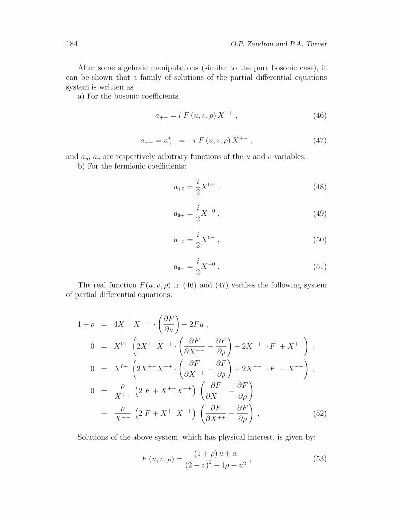
After some algebraic manipulations (similar to the pure bosonic case), itcan be shown that a family of solutions of the partial differential equationssystem is written as:
a) For the bosonic coefficients:
a+− = i F (u, v, ρ)X−+ , (46)
a−+ = a∗+− = −i F (u, v, ρ)X+− , (47)
and au, av are respectively arbitrary functions of the u and v variables.b) For the fermionic coefficients:
a+0 =i
2X0+ , (48)
a0+ =i
2X+0 , (49)
a−0 =i
2X0− , (50)
a0− =i
2X−0 . (51)
The real function F (u, v, ρ) in (46) and (47) verifies the following systemof partial differential equations:
1 + ρ = 4X+−X−+ ·(∂F
∂u
)− 2Fu ,
0 = X0+
(2X+−X−+ ·
(∂F
∂X−−− ∂F
∂ρ
)+ 2X++ · F +X++
),
0 = X0+
(2X+−X−+ ·
(∂F
∂X++− ∂F
∂ρ
)+ 2X−− · F −X−−
),
0 =ρ
X++
(2 F +X+−X−+
) ( ∂F
∂X−−− ∂F
∂ρ
)
+ρ
X−−
(2 F +X+−X−+
) ( ∂F
∂X++− ∂F
∂ρ
), (52)
Solutions of the above system, which has physical interest, is given by:
F (u, v, ρ) =(1 + ρ)u+ α
(2− v)2 − 4ρ− u2, (53)

First order Lagrangians and path integral quantization ... 185
being α an arbitrary and non-trivial integration constant. In the bosonic limitwhen ρ = 0 and v = 1 it results:
F (u) =u+ α
1− u2, (54)
it recovers the solution for the pure bosonic case [14]-[17].For simplicity, we choose a particular family of solutions by taking au =
av = 0 and α = −1, so the Lagrangian (38) is written as:
L(X, X) = i∑i
ui (1 + ρi)− 1
(2− vi)2 − (4ρi + u2i )
(X−+i X+−
i −X+−i X−+
i
)+
i
2
∑i,σ
(Xσ0i X
0σi +X0σ
i Xσ0i
)−Ht−J(X) , (55)
where σ takes the values + and −, and the site index i was added. In (55) theHamiltonian for the t-J model in terms of the Hubbard operators is given by:
Ht−J(X) =∑i,j,σ
tij(Xσ0i X
0σj
)+
1
4
∑i,j,σ,γ
Jij(Xσγi Xγσ
j
)− 1
4
∑i,j,σ,η
Jij(Xσηi Xση
j
). (56)
4 Spinless Fermion Representation
The treatment of the spinless fermion model is useful for to understand how thealgorithm is applied when boson-like and fermion-like Hubbard X-operatorsare present, and to show that the path-integral representation produces anadequate generating correlation functional of the model.
Our purpose is to construct a family of classical first-order Lagrangianswritten in terms of the Hubbard X-operators whose graded quantum Diracbrackets between field variables are given by (1). This approach shows howthe constraint structure and the number of constraints present are provided bythe symplectic Faddeev-Jackiw quantum method. We assume that the classicalfirst-order Lagrangian, idem (16), can be written as:
L = aαβ(X)Xαβ − V 0 . (57)
In the Faddeev-Jackiw language the symplectic potential V 0 is defined by:
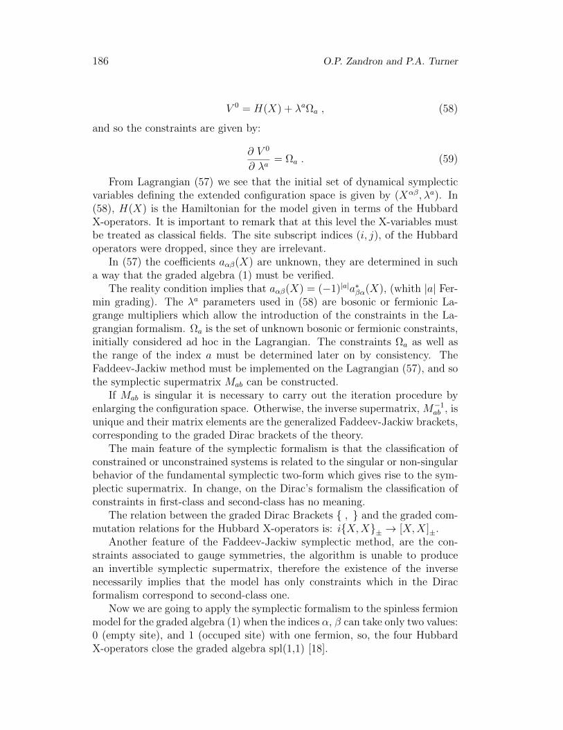
186 O.P. Zandron and P.A. Turner
V 0 = H(X) + λaΩa , (58)
and so the constraints are given by:
∂ V 0
∂ λa= Ωa . (59)
From Lagrangian (57) we see that the initial set of dynamical symplecticvariables defining the extended configuration space is given by (Xαβ, λa). In(58), H(X) is the Hamiltonian for the model given in terms of the HubbardX-operators. It is important to remark that at this level the X-variables mustbe treated as classical fields. The site subscript indices (i, j), of the Hubbardoperators were dropped, since they are irrelevant.
In (57) the coefficients aαβ(X) are unknown, they are determined in sucha way that the graded algebra (1) must be verified.
The reality condition implies that aαβ(X) = (−1)|a|a∗βα(X), (whith |a| Fer-min grading). The λa parameters used in (58) are bosonic or fermionic La-grange multipliers which allow the introduction of the constraints in the La-grangian formalism. Ωa is the set of unknown bosonic or fermionic constraints,initially considered ad hoc in the Lagrangian. The constraints Ωa as well asthe range of the index a must be determined later on by consistency. TheFaddeev-Jackiw method must be implemented on the Lagrangian (57), and sothe symplectic supermatrix Mab can be constructed.
If Mab is singular it is necessary to carry out the iteration procedure byenlarging the configuration space. Otherwise, the inverse supermatrix, M−1
ab , isunique and their matrix elements are the generalized Faddeev-Jackiw brackets,corresponding to the graded Dirac brackets of the theory.
The main feature of the symplectic formalism is that the classification ofconstrained or unconstrained systems is related to the singular or non-singularbehavior of the fundamental symplectic two-form which gives rise to the sym-plectic supermatrix. In change, on the Dirac’s formalism the classification ofconstraints in first-class and second-class has no meaning.
The relation between the graded Dirac Brackets , and the graded com-mutation relations for the Hubbard X-operators is: iX,X± → [X,X]±.
Another feature of the Faddeev-Jackiw symplectic method, are the con-straints associated to gauge symmetries, the algorithm is unable to producean invertible symplectic supermatrix, therefore the existence of the inversenecessarily implies that the model has only constraints which in the Diracformalism correspond to second-class one.
Now we are going to apply the symplectic formalism to the spinless fermionmodel for the graded algebra (1) when the indices α, β can take only two values:0 (empty site), and 1 (occuped site) with one fermion, so, the four HubbardX-operators close the graded algebra spl(1,1) [18].
First order Lagrangians and path integral quantization ... 187
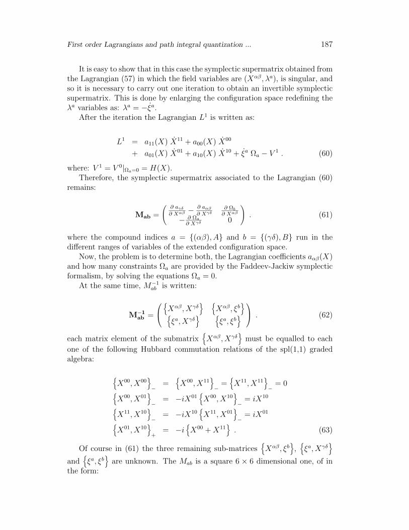
It is easy to show that in this case the symplectic supermatrix obtained fromthe Lagrangian (57) in which the field variables are (Xαβ, λa), is singular, andso it is necessary to carry out one iteration to obtain an invertible symplecticsupermatrix. This is done by enlarging the configuration space redefining theλa variables as: λa = −ξa.
After the iteration the Lagrangian L1 is written as:
L1 = a11(X) X11 + a00(X) X00
+ a01(X) X01 + a10(X) X10 + ξa Ωa − V 1 . (60)
where: V 1 = V 0|Ωa=0 = H(X).Therefore, the symplectic supermatrix associated to the Lagrangian (60)
remains:
Mab =
(∂ aγδ∂ Xαβ − ∂ aαβ
∂ Xγδ∂ Ωb∂ Xαβ
− ∂ Ωa∂ Xγδ 0
). (61)
where the compound indices a = (αβ), A and b = (γδ), B run in thedifferent ranges of variables of the extended configuration space.
Now, the problem is to determine both, the Lagrangian coefficients aαβ(X)and how many constraints Ωa are provided by the Faddeev-Jackiw symplecticformalism, by solving the equations Ωa = 0.
At the same time, M−1ab is written:
M−1ab =
Xαβ, Xγδ
Xαβ, ξb
ξa, Xγδ
ξa, ξb
. (62)
each matrix element of the submatrixXαβ, Xγδ
must be equalled to each
one of the following Hubbard commutation relations of the spl(1,1) gradedalgebra:
X00, X00
−
=X00, X11
−
=X11, X11
−
= 0X00, X01
−
= −iX01X00, X10
−
= iX10X11, X10
−
= −iX10X11, X01
−
= iX01X01, X10
+
= −iX00 +X11
. (63)
Of course in (61) the three remaining sub-matricesXαβ, ξb
,ξa, Xγδ
and
ξa, ξb
are unknown. The Mab is a square 6 × 6 dimensional one, of in
the form:

188 O.P. Zandron and P.A. Turner
Mab =(Abb Bbf
Cfb Dff
). (64)
whose Bose-Bose parts Abb and Fermi-Fermi parts Dff are even elementsof the Grassmann algebra and whose Bose-Fermi parts Bbf and Fermi-Boseparts Cfb are odd elements. The inverse M−1
ab exists if and only if Abb and Dff
have an inverse [19]. The Bose-Bose part Abb is an ordinary non-singular 4× 4dimensional matrix and the Fermi-Fermi part Dff is an ordinary non-singular
2 × 2 dimensional matrix. By using the equation Mab
(M bc
)−1= δca, and
taking into account the equation:(M bc
)−1= −i(−1)|εb| [b, c]± , (65)
where |εb| is the Fermi grading of the variable b, differential equations on theLagrangian coefficients aαβ and on the constraints Ωa are obtained.
The system of four homogeneous differential equations on the constraintsΩa can be written:
i(−1)|εαβ |(|a|+1) ∂ Ωa
∂ Xαβ
[Xαβ, Xγδ
]±
= 0 , (66)
where |εαβ| and |a| are the Fermi grading of the Hubbard operators and of theconstraints respectively.
Solving the differential equations system (66), two bosonic solutions arefound. So, the associated constraints read:
Ω1 = X00 +X11 − 1 = 0 , (67)
Ω2 = X11 +X01X10 − 1 = 0 , (68)
Alleged the invertibility of the supermatrix (61), necessarily the constraints(67) and (68) are second-class, as really occurs.
On the other hand, by solving the remaining system of the differentialequations on the Lagrangian coefficients aαβ, the values are:
a00 =1
2X11, a11 = −1
2X00, a10 =
i
2X01, a01 =
i
2X10 , (69)
The constraint (67) provided by the Faddeev-Jackiw symplectic formal-ism is the completeness condition (2), which is necessary due to the ban thedouble occupancy at each site.
Consequently, from the Lagrangian (57), the coefficients given in (69) andthe bosonic constraints (67) and (68), it is possible to prove that the gradedalgebra spl(1.1) given in (63) is recovered.
First order Lagrangians and path integral quantization ... 189
Now, we can to write the generating functional correlation by using thepath-integral approach of Faddeev-Senjanovich [20]-[21]. Thus, the spinlessfermion model initially partition function can be written as:
Z =∫
DXδ(X01X10 +X11 − 1
)δ(X11 +X00 − 1
)exp
(i∫
L(X, X
)dt),
(70)where the Lagrangian L(X, X) is:
L =1
2
(X11X00 −X00X11
)+i
2
(X01X10 +X10X01
)−H(X) . (71)
In (70) the superdeterminant of the supermatrix with structed was omittedfrom the constraints field because it is independent and can be included in thepath-integral normalization factor.
By integrating out the bosonic variablesX11 andX00, the partition function(70) is:
Z =∫
DX10DX01 exp(i∫
Leff(X, X
)dt), (72)
where:
Leff(X, X
)=i
2
(X01X10 +X10X01
)−H(X)|Ωa=0 . (73)
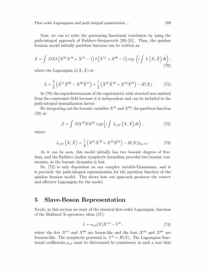
As it can be seen, this model initially has two bosonic degrees of free-dom, and the Faddeev-Jackiw symplectic formalism provides two bosonic con-straints, so the bosonic dynamics is lost.
So, (72) is only dependent on one complex variable-Grassmann, and itis precisely the path-integral representation for the partition function of thespinless fermion model. This shows how our approach produces the correctand effective Lagrangian for the model.
5 Slave-Boson Representation
Newly, in this section we start of the classical first-order Lagrangian, functionof the Hubbard X-operators, idem (57):
L = aαβ(X)Xαβ − V 0 . (74)
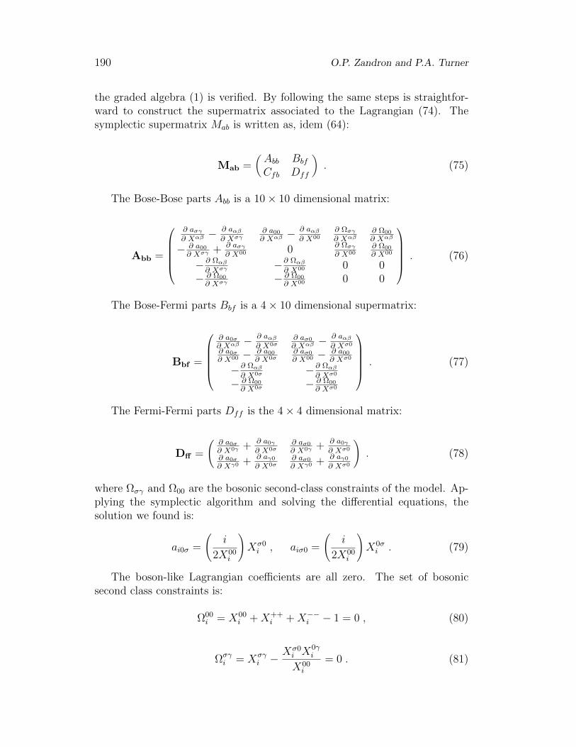
where the five Xσγ and X00 are boson-like and the four Xσ0 and X0σ arefermion-like. The symplectic potential is: V 0 = H(X). The Lagrangian func-tional coefficients aαβ must be determined by consistency in such a way that
190 O.P. Zandron and P.A. Turner
the graded algebra (1) is verified. By following the same steps is straightfor-ward to construct the supermatrix associated to the Lagrangian (74). Thesymplectic supermatrix Mab is written as, idem (64):
Mab =(Abb Bbf
Cfb Dff
). (75)
The Bose-Bose parts Abb is a 10× 10 dimensional matrix:
Abb =
∂ aσγ∂ Xαβ − ∂ aαβ
∂ Xσγ∂ a00∂ Xαβ − ∂ aαβ
∂ X00
∂ Ωσγ∂ Xαβ
∂ Ω00
∂ Xαβ
− ∂ a00∂ Xσγ + ∂ aσγ
∂ X00 0 ∂ Ωσγ∂ X00
∂ Ω00
∂ X00
− ∂ Ωαβ∂ Xσγ −∂ Ωαβ
∂ X00 0 0− ∂ Ω00
∂ Xσγ − ∂ Ω00
∂ X00 0 0
. (76)
The Bose-Fermi parts Bbf is a 4× 10 dimensional supermatrix:
Bbf =
∂ a0σ∂ Xαβ − ∂ aαβ
∂ X0σ∂ aσ0∂ Xαβ − ∂ aαβ
∂ Xσ0
∂ a0σ∂ X00 − ∂ a00
∂ X0σ∂ aσ0∂ X00 − ∂ a00
∂ Xσ0
− ∂ Ωαβ∂ X0σ − ∂ Ωαβ
∂ Xσ0
− ∂ Ω00
∂ X0σ − ∂ Ω00
∂ Xσ0
. (77)
The Fermi-Fermi parts Dff is the 4× 4 dimensional matrix:
Dff =
(∂ a0σ∂ X0γ + ∂ a0γ
∂ X0σ∂ aσ0∂ X0γ + ∂ a0γ
∂ Xσ0
∂ a0σ∂ Xγ0 + ∂ aγ0
∂ X0σ∂ aσ0∂ Xγ0 + ∂ aγ0
∂ Xσ0
). (78)
where Ωσγ and Ω00 are the bosonic second-class constraints of the model. Ap-plying the symplectic algorithm and solving the differential equations, thesolution we found is:
ai0σ =
(i
2X00i
)Xσ0i , aiσ0 =
(i
2X00i
)X0σi . (79)
The boson-like Lagrangian coefficients are all zero. The set of bosonicsecond class constraints is:
Ω00i = X00
i +X++i +X−−i − 1 = 0 , (80)
Ωσγi = Xσγ
i −Xσ0i X
0γi
X00i
= 0 . (81)
First order Lagrangians and path integral quantization ... 191
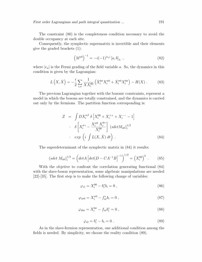
The constraint (80) is the completeness condition necessary to avoid thedouble occupancy at each site.
Consequently, the symplectic supermatrix is invertible and their elementsgive the graded brackets (1):(
Mab)−1
= −i(−1)|εa| [a, b]± , (82)
where |εa| is the Fermi grading of the field variable a. So, the dynamics in thiscondition is given by the Lagrangian:
L(X, X
)= − i
2
∑i,σ
1
XX00i
(X0σi X
σ0i + Xσ0
i X0σi
)−H(X) . (83)
The previous Lagrangian together with the bosonic constraints, represent amodel in which the bosons are totally constrained, and the dynamics is carriedout only by the fermions. The partition function corresponding is:
Z =∫DXαβ
i δ[X00i +X++
i +X−−i − 1]
· δ
[Xσγi −
Xσ0i X0γ
i
X00i
](sdetMab)
1/2i
· exp(i∫L(X, X) dt
). (84)
The superdeterminant of the symplectic matrix in (84) it results:
(sdet Mab)1/2i =
(detA
[det(D − CA−1B
]−1)1/2
=(X00i
)2. (85)
With the objetive to confront the correlation generating functional (84)with the slave-boson representation, some algebraic manipulations are needed[22]-[35]. The first step is to make the following change of variables:
ϕi1 = X00i − b∗i bi = 0 , (86)
ϕiσ0 = Xσ0i − f ∗iσbi = 0 , (87)
ϕi0σ = X0σi − fiσb∗i = 0 , (88)
ϕi2 = b∗i − bi = 0 . (89)
As in the slave-fermion representation, one additional condition among thefields is needed. By simplicity, we choose the reality condition (89).

192 O.P. Zandron and P.A. Turner
The super Jacobian Ji of the transformation (86)-(89) is:
Ji = −b∗i + bi
(b∗i bi)2 . (90)
Now, by introducing in the equation (84) the unity:
1 =∫
Df ∗iσ Dfiσ Db∗i Dbi Ji δ
(Xσ0i − f ∗iσ bi
)δ(X0σi − fiσ b∗i
)· δ
(b∗i bi −X00
i
)δ (b∗i − bi) . (91)
Integrating out all the fields, is possible to show that the partition functionZ takes the form:
Z =∫Db∗i Dbi Df
∗iσ Dfiσ δ (Ωi) δ (φi) (b∗i + bi)
· exp(i∫L(b∗, b, f ∗σ , fσ) dt
), (92)
where Ωi and ϕi are the first-class constraint and the gauge fixing conditionappearing in the partition function of the slave-boson representation. Theyrespectively read:
Ωi = b∗i bi +∑iσ
f ∗iσ fiσ − 1 = 0 , (93)
φi = i (bi − b∗i ) = 0 . (94)
We note that the factor (b+ b∗) in the equation (92) is precisely the valueof the det [Ωi, ϕi]D of the gauge theories with first-class constraints. TheLagrangian in (92) is given by:
L(b∗, b, f ∗σ , fσ) =1
2i∑i
(b∗i bi − b∗i bi
)+
1
2i∑iσ
(f ∗iσ fiσ − f ∗iσ fiσ
)−H . (95)
From our approach, with the Hubbard X-operators and without any decou-pling, the Lagrangian (83) is obtained. The functional (84) is mapped into thesolution provided by the slave-boson representation. It is important to notethat the new path-integral (84) in terms of the Hubbard X-operators was de-veloped. We see how a second-class constrained model written in terms of theHubbard X-operators in terms of the decoupled slave-particle representations,is transformed in a constrained system. The local gauge symmetry is evident.We think that the equation (84) with the Lagrangian (83) can be useful forregimes where the system is close to a Fermi liquid state.
First order Lagrangians and path integral quantization ... 193
6 Path-Integral Representation
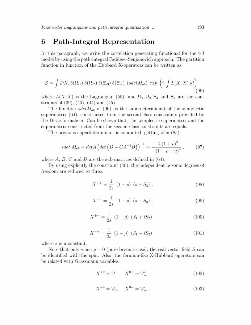
In this paragraph, we write the correlation generating functional for the t-Jmodel by using the path-integral Faddeev-Senjanovich approach. The partitionfunction in function of the Hubbard X-operators can be written as:
Z =∫DXi δ(Ωi1) δ(Ωi2) δ(Ξi3) δ(Ξi4) (sdetMab) exp
(i∫L(X, X) dt
),
(96)where L(X, X) is the Lagrangian (55), and Ω1,Ω2,Ξ3 and Ξ4 are the con-straints of (39), (40), (44) and (45).
The function sdetMab of (96), is the superdeterminant of the symplecticsupermatrix (64), constructed from the second-class constraints provided bythe Dirac formalism. Can be shown that, the symplectic supermatrix and thesupermatrix constructed from the second-class constraints are equals.
The previous superdeterminant is computed, getting iden (85):
sdet Mab = detA(det
(D − CA−1B
))−1= − 4 (1 + ρ)2
(1− ρ+ u)2 , (97)
where A, B, C and D are the sub-matrices defined in (64).By using explicitly the constraint (40), the independent bosonic degrees of
freedom are reduced to three:
X++ =1
2s(1− ρ) (s+ S3) , (98)
X−− =1
2s(1− ρ) (s− S3) , (99)
X+− =1
2s(1− ρ) (S1 + iS2) , (100)
X−+ =1
2s(1− ρ) (S1 − iS2) , (101)
where s is a constant.Note that only when ρ = 0 (pure bosonic case), the real vector field S can
be identified with the spin. Also, the fermion-like X-Hubbard operators canbe related with Grassmann variables:
X+0 = Ψ− X0+ = Ψ∗− , (102)
X−0 = Ψ+ X0− = Ψ∗+ , (103)

194 O.P. Zandron and P.A. Turner
where now ρ = Ψ∗+Ψ+ + Ψ∗−Ψ− and accounting the fermionic constraints (42)-(45) it results (1− ρ) (1 + ρ) = 1.
The remaining bosonic constraint (40) as function of the real vector fieldvariable S writes:
Ω2 = S21 + S2
2 + S23 − s = 0 , (104)
and, the two fermionic constraints (44) and (45) can be written:
Ξ3 = Ψ∗− (S1 + iS2)−Ψ∗+ (s+ S3) = 0 , (105)
Ξ4 = Ψ− (S1 − iS2)−Ψ+ (s+ S3) = 0 . (106)
Unless of a total time derivative the Lagrangian (55) in terms of these newfields is:
L =1
2s
∑i
(Si2Si1 − Si1Si2
)s+ Si3
+ i∑iσ
(Ψiσ Ψ∗iσ
)−Ht−J . (107)
The Ht−J of (107) written in term of S and the component spinors (102)and (103), is:
Ht−J =∑ijσ
tij Ψ∗jσ Ψiσ
+∑ij
Jij8s2
(1− ρi) (1− ρj)(Si1Sj1 + Si2Sj2 + Si3Sj3 − s2
)(108)
Finally, we note that the fermionic constraints (42)-(45), in matrix nota-tion, are:
Ξ∗ = Ψ∗ (sI + S · σ) = 0 , (109)
Ξ = (sI + S · σ) Ψ = 0 , (110)
where σ are the Pauli matrices, and the two-component spinor Ψ = (−Ψ+,Ψ−),this constraints are those used in the framework of the coherent state repre-sentation.
By using the integral representation for the delta functions, (96) can bewritten in an alternative way, the delta functions is: δ(Φ) =
∫Dχ exp (i
∫χ Φ dt),
where the quantities χ are suitable bosonic or fermionic Lagrange multipliers.So, the functional (96) takes the form:

First order Lagrangians and path integral quantization ... 195
Z =∫DXi D(λ1
i ) D(λ2i ) D(ξi) D(ξ∗i ) (sdetMab) exp
(i∫Leff (X, X) dt
).
(111)The Leff (X, X) in (111) is defined by:
Leff (X, X) = L(X, X) +∑i
λ1i
(X++i +X−−i + ρi − 1
)+
∑i
λ2i
(X+−i X−+
i +1
4u2i −
(1− 1
2vi
)2
+ ρi
)+
(X0+i X+−
i −X0−i X++
i
)ξi
+ ξ∗i(X+0i X−+
i −X−0i X++
i
), (112)
where L(X, X) was given in (55).In (112) the parameters λa with (a = 1, 2) and ξ are respectively bosonic
and fermionic Lagrange multipliers. The sdetMab in terms of the S and thetwo component spinor Ψ results:
sdet Mab = − 4s2(1 + ρ)2
(1− ρ)2(s+ S3)2. (113)
The exponentiation of the superdeterminant is realized by introducing theFaddeev-Popov ghosts in the effective Lagrangian. Consequently, the func-tional sdetMab is:
sdet M =∫
DC exp i(Ca
1 Mab Cb2
), (114)
where DC = Πa DCa2 DC
a1 and Ca
A (A = 1, 2) denote commuting as well asanti-commuting ghosts. Using the transformations (98)-(103), (111) is:
Z =∫DSi1 DSi2 DSi3 DΨiσ DΨ∗iσ Dλ
2i Dξi Dξ
∗i
· (sdetMab)∂X
∂Sexp
(i∫Leff (X, X) dt
), (115)
where the quantity ∂X/∂S is the super Jacobian of the transformation. Thefield is:
∂X
∂S= −i (1− ρ)3
2s3. (116)
The Leff in (115), in terms of the new variables is:
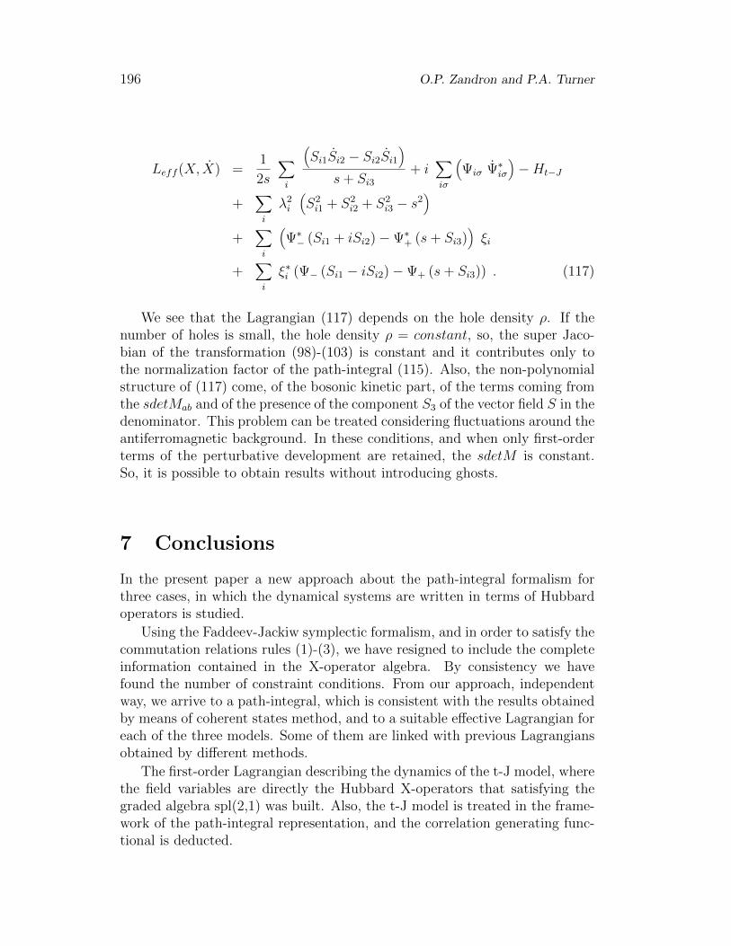
196 O.P. Zandron and P.A. Turner
Leff (X, X) =1
2s
∑i
(Si1Si2 − Si2Si1
)s+ Si3
+ i∑iσ
(Ψiσ Ψ∗iσ
)−Ht−J
+∑i
λ2i
(S2i1 + S2
i2 + S2i3 − s2
)+
∑i
(Ψ∗− (Si1 + iSi2)−Ψ∗+ (s+ Si3)
)ξi
+∑i
ξ∗i (Ψ− (Si1 − iSi2)−Ψ+ (s+ Si3)) . (117)
We see that the Lagrangian (117) depends on the hole density ρ. If thenumber of holes is small, the hole density ρ = constant, so, the super Jaco-bian of the transformation (98)-(103) is constant and it contributes only tothe normalization factor of the path-integral (115). Also, the non-polynomialstructure of (117) come, of the bosonic kinetic part, of the terms coming fromthe sdetMab and of the presence of the component S3 of the vector field S in thedenominator. This problem can be treated considering fluctuations around theantiferromagnetic background. In these conditions, and when only first-orderterms of the perturbative development are retained, the sdetM is constant.So, it is possible to obtain results without introducing ghosts.
7 Conclusions
In the present paper a new approach about the path-integral formalism forthree cases, in which the dynamical systems are written in terms of Hubbardoperators is studied.
Using the Faddeev-Jackiw symplectic formalism, and in order to satisfy thecommutation relations rules (1)-(3), we have resigned to include the completeinformation contained in the X-operator algebra. By consistency we havefound the number of constraint conditions. From our approach, independentway, we arrive to a path-integral, which is consistent with the results obtainedby means of coherent states method, and to a suitable effective Lagrangian foreach of the three models. Some of them are linked with previous Lagrangiansobtained by different methods.
The first-order Lagrangian describing the dynamics of the t-J model, wherethe field variables are directly the Hubbard X-operators that satisfying thegraded algebra spl(2,1) was built. Also, the t-J model is treated in the frame-work of the path-integral representation, and the correlation generating func-tional is deducted.

First order Lagrangians and path integral quantization ... 197
Using the supersymmetric version of the Faddeev-Jackiw formalism, sam-ple that it is possible to find a family of first-order Lagrangian able to repro-duce at classical level the generalized Faddeev-Jackiw brackets or graded Diracbrackets of the t-J model. When the transition is realized in a canonical quan-tum formalism, the graded quantum Dirac brackets are precisely the gradedcommutators of the Hubbard X-operators algebra, and in both cases, for thespinless fermion model as well as for the t-J model, the unique possible set ofconstraints is naturally provided by the symplectic Faddeev-Jackiw method.
By last, the pure bosonic case in a classical Lagrangian formalism was an-alyzed. In this case, it is not possible to introduce the full Hubbard algebraby means of constraints. So, in a path-integral formulation it cannot be in-troduced the complete information of the algebra, namely, the commutationrules, the completeness condition and the multiplication rules for the opera-tors. The Heisenberg model treated under Lagrangian formalism only admitstwo second-class constraints, the completeness condition and the non-linearconstraint. It can be shown that the presence of such constraint is consistentwith the quantization of a spin system in the limit of large spin, or equivalentlyfor magnetic order state.
A similar situation occurs when the Hubbard X-operators closes the gradedalgebra spl(2,1), the t-J model described in terms of a first-order Lagrangiansupports two possible solutions: the first solution is the family of first-orderLagrangians together with the set of second-class constraints, two are bosonicsand two are fermionics. In particular the constraint (80) is the completenesscondition. So, the path-integral formalism is mapped into the decoupled slave-fermion representation, in this case, our correlation generating functional (70)privilege the magnon dynamics of the system with a strong feature of magneticorder state. The second solution, is the new set of second-class constraints,in this case all the constraints are bosonic, and (80) is again the complete-ness condition. In this situation the bosons are totally constrained, and thedynamics is carried out only by the fermions. The path-integral formalismcorresponds to the situation of the slave-boson representation, therefore, inour correlation generating functional (84) the fermion dynamics with a strongfeature of Fermi liquid, is privileged.
We conclude that once the set of second class-constraints is chosen, differentLagrangians are obtained, and we can insure that each one contains differentphysics. Worthwhile to remark that both of them Lagrangian formalism areindependent of the dimension of the lattice. Moreover, as it was seen in allthe cases the completeness condition appears as necessary. The completenesscondition involve an important physical meaning, such condition avoids at thequantum level the double occupancy at each lattice site.
198 O.P. Zandron and P.A. Turner
References
[1] J. Hubbard, Electron Correlations in Narrow Energy Bands, Proc. R. Soc.A, 276 (1963), 238-257. http://dx.doi.org/10.1098/rspa.1963.0204
[2] J. Hubbard, Electron Correlations in Narrow Energy Bands II. The de-generate band case, Proc. R. Soc. A, 277 (1964), 237-259.http://dx.doi.org/10.1098/rspa.1964.0019
[3] J. Hubbard, Electron Correlations in Narrow Energy Bands III. An Im-proved Solution, Proc. R. Soc. A, 284 (1964), 401-419.http://dx.doi.org/10.1098/rspa.1964.0190
[4] A. Izyumov and N. Skryabin, Statistical Mechanics of Magnetically Or-dered Systems, Consultants Bureau, New York, 1988.
[5] L.D. Faddeev and R. Jackiw, Hamiltonian reduction of unconstrained andconstrained systems, Phys. Rev. Lett., 60 (1988), 1692-1694.http://dx.doi.org/10.1103/physrevlett.60.1692
[6] J. Barcelos Neto and C. Wotzasek, Faddeev-Jackiw quantization and con-straints, Int. Jour. Mod. Phys. A, 7 (1992), 4981-5003.http://dx.doi.org/10.1142/s0217751x9200226x
[7] H. Montani and C. Wotzasek, Faddeev-Jackiw quantization of non-Abelian systems, Mod. Phys. Lett. A, 8 (1993), 3387-3396.http://dx.doi.org/10.1142/s0217732393003810
[8] P.A.M. Dirac, Lectures on Quantum Mechanics, Yeshiva University Press,New York, 1964.
[9] J.C. Le Guillou and E. Ragoucy, Slave-particle quantization and sum rulesin the t-J model, Phys. Rev. B, 52 (1995), 2403-2414.http://dx.doi.org/10.1103/physrevb.52.2403
[10] A. Izyumov, Strongly correlated electrons: the t-J model, Physics-Uspekhi, 40 (1997), 445-476.http://dx.doi.org/10.1070/pu1997v040n05abeh000234
[11] A. Greco and R. Zeyher, Superconducting instabilities in the tt’ Hub-bard model in the large-N limit, Europhys. Lett., 35 (1996), 115-120.http://dx.doi.org/10.1209/epl/i1996-00541-0
[12] P.B. Wiegmann, Superconductivity in strongly correlated electronic sys-tems and confinement versus deconfinement phenomenon, Phys. Rev.Lett., 60 (1988), 821-824. http://dx.doi.org/10.1103/physrevlett.60.821
First order Lagrangians and path integral quantization ... 199
[13] P.B. Wiegmann, Extrinsic geometry of superstrings, Nucl. Phys. B, 323(1989), 330-336. http://dx.doi.org/10.1016/0550-3213(89)90145-4
[14] A. Jevicki and N. Papanicolau, Semi-classical spectrum of the continuousHeisenberg spin chain, Ann. Phys., 120 (1979), 107-128.http://dx.doi.org/10.1016/0003-4916(79)90283-5
[15] M.W. Kirson, A Dynamical Supersymmetry in the Hubbard Model, Phys.Rev. Lett., 78 (1997), 4241-4244.http://dx.doi.org/10.1103/physrevlett.78.4241
[16] J. Govaerts, Hamiltonian reduction of first-order actions, Int. Jour. Mod.Phys. A, 5 (1990), 3625-3640.http://dx.doi.org/10.1142/s0217751x90001574
[17] A. Foussats, C. Repetto, O.P. Zandron and O.S. Zandron, Supersymmet-ric anyons in the Faddeev-Jackiw quantization picture, Ann. Phys., 268(1998), 225-245. http://dx.doi.org/10.1006/aphy.1998.5823
[18] D. Foster, Decoupling of holes in the t-J model at J=2t from spl(2,1)symmetry, Zeitschrift fur Physik B Condensed Matter, 82 (1991), 329-334. http://dx.doi.org/10.1007/bf01357174
[19] P. Van Nieuwenhuizen, Supergravity, Phys. Rep., 68 (1981), 189-389.http://dx.doi.org/10.1016/0370-1573(81)90157-5
[20] L.D. Faddeev, The Feynman integral for singular Lagrangians, Theor.Math. Phys., 1 (1970), 1-13. http://dx.doi.org/10.1007/bf01028566
[21] P. Senjanovic, Path integral quantization of field theories with second-class constraints, Ann. Phys., 100 (1976), 227-261.http://dx.doi.org/10.1016/0003-4916(76)90062-2
[22] A. Angelucci, Effective lattice actions for correlated electrons, PhysicalReview B, 51 (1995), 11580-11583.http://dx.doi.org/10.1103/physrevb.51.11580
[23] A.J. Bracken, M.D. Gould, J.R. Links and Y.Z. Zhang, New supersym-metric and exactly solvable model of correlated electrons, Phys. Rev. Lett.,74 (1995), 2768-2771. http://dx.doi.org/10.1103/physrevlett.74.2768
[24] Z. Maassarani, U q osp(2,2) lattice models, J. Phys. A, 28 (1995), 1305-1323. http://dx.doi.org/10.1088/0305-4470/28/5/017
[25] M.J. Martins and P.B. Ramos, Solution of a supersymmetric model ofcorrelated electrons, Physical Review B, 56 (1997), 6376-6379.http://dx.doi.org/10.1103/physrevb.56.6376
200 O.P. Zandron and P.A. Turner
[26] S. Sarkar, The supersymmetric t-J model in one dimension, Journal ofPhysics A, 24 (1991), 1137-1151.http://dx.doi.org/10.1088/0305-4470/24/5/026
[27] A. Angelucci and R. Link, Graded Holstein-Primakoff transformationsand the semiclassical limit of strongly correlated electron systems, Phys.Rev. B, 46 (1992), 3089-3094.http://dx.doi.org/10.1103/physrevb.46.3089
[28] A. Forster and M. Karowski, Algebraic properties of the Bethe ansatz foran spl(2,1) supersymmetric t-J model, Nucl. Phys B, 396 (1993), 611-638.http://dx.doi.org/10.1016/0550-3213(93)90665-c
[29] T.K. Ng and C.H. Cheng, Supersymmetry in models with strong on-siteCoulomb repulsion, application to t-J model, HKUST, Kowloon, HongKong, 1998.
[30] G. Baskaran, Z. Zou and P.W. Anderson, The resonating valencebond state and high-Tc superconductivity - A mean field theory, SolidState Commun., 63 (1987), 973-976. http://dx.doi.org/10.1016/0038-1098(87)90642-9
[31] G. Kotliar and J. Liu, Superexchange mechanism and d-wave supercon-ductivity, Phys. Rev. B, 38 (1988), 5142-5145.http://dx.doi.org/10.1103/physrevb.38.5142
[32] C. Jayaprakash, H.R. Krishnamurthy and S. Sarker, Mean-field theory forthe t-J model, Phys. Rev. B, 40 (1989), 2610-2613.http://dx.doi.org/10.1103/physrevb.40.2610
[33] C.L. Kane, P.A. Lee, T.K. Ng, B. Chakraborty and N. Read, Mean-fieldtheory of the spiral phases of a doped anti-ferromagnet, Phys. Rev. B, 41(1990), 2653-2656. http://dx.doi.org/10.1103/physrevb.41.2653
[34] J.R. Klauder, Coherent State Quantization of Constraint Systems, Ann.Phys., 254 (1997), 419-453. http://dx.doi.org/10.1006/aphy.1996.5647
[35] E. Tungler and T. Kopp, Functional integrals for Hubbard operators andprojection methods for strong interaction, Preprint Institut fur Theorieder Kondensierten Materie, Universitat Karlsruhe (1999).
Received: January 9, 2016; Published: April 19, 2016