first-principles thermal conductivity of deuterium for

First-PrinciPles thermal conductivity oF deuterium For inertial conFinement Fusion aPPlications

LLE Review, Volume 137 81

IntroductionAs a grand challenge to harvest the “ultimate” energy source in a controlled fashion, inertial confinement fusion (ICF)1 has been actively pursued for decades using both indirect-drive2,3

and direct-drive4–6 configurations. Understanding and design-ing ICF capsule implosions rely on simulations using multi-physics radiation–hydrodynamics codes, in which each piece of the physics models must be accurate. According to the ICF ignition criterion,7,8 the minimum laser energy required for ignition scales as

,E V

P590

3 10100kJ Mbar

0.8.

.1 9

7 6 6

Limp

a# #

##- a

-

_ f fi p p (1)

where the implosion velocity Vimp is in cm/s, Pa is the ablation pressure in Mbar, and the DT shell’s adiabat a is convention-ally defined as a = P/PF, the ratio of plasma pressure to the Fermi-degeneracy pressure (PF). This scaling law indicates that the lower the shell adiabat, the less energy needed for igni-tion. For lower-a implosions, however, the DT shell is in the regime in which strong coupling and degeneracy plasma effects are important and must be taken into account for meaningful implosion modeling.

The determination of accurate plasma properties is also very important for understanding low-adiabat (a # 2) ICF implosions. Precise knowledge of the static and dynamic properties of ICF target materials, including ablators and the deuterium–tritium (DT) fuel, is required under high-energy-density conditions. For instance, the equation of state (EOS) of the target materials determines how much compression can be attained under external pressures generated by x-ray/laser ablations.9 For this exact reason, state-of-the-art EOS experiments and calculations have been performed for ICF-relevant materials10–16 over the past few years. The theoretical approaches have employed first-principles methods such as the path-integral Monte Carlo (PIMC),17 coupled electron–ion Monte Carlo (CEIMC),18 and quantum molecular dynamics

First-Principles Thermal Conductivity of Deuterium for Inertial Confinement Fusion Applications

(QMD)19 based on the finite-temperature density-functional theory. Besides static EOS information, the dynamic transport properties of relevant materials are in high demand for accurate ICF simulations. Transport and optical properties (thermal and electrical conductivities) of DT and ablators not only affect the thermal conduction, but also determine the radiation transport in the imploding shell.

Soon after the introduction of the ICF concept1 in 1972, studies followed to determine the most-appropriate models for thermal conductivity of strongly coupled and degenerate plas-mas in the high-density, low-temperature regime.20 The Spitzer model21 of thermal conductivity l, formulated in the 1950s for ideal plasmas, breaks down in this regime since the Coulomb logarithm22–26 for electron–ion collisions becomes negative. Brysk et al.20 suggested in the 1970s that the Hubbard model27 of degenerate plasma be “bridged” with the Spitzer model.21 In the 1980s, Lee and More28 applied Krook’s model to the Boltzman equation and derived a set of transport coefficients, including l. Meanwhile, Ichimaru and colleagues29 developed the so-called “Ichimaru model” of thermal conductivity for fully ionized plasmas using the linear response theory. In addi-tion, the average-atom model30 and its improved versions have been used to numerically calculate l for materials of interest to ICF and astrophysics, with tools such as the PURGATORIO package31 and the SCAALP model.32 As a result of recent progress in the first-principles method of quantum molecular dynamics,33–37 these various thermal-conductivity models of hydrogen/DT have been tested against QMD calculations.38–43 For ICF stagnation plasma conditions near peak compression, the pioneering QMD calculations by Recoules et al.38 have shown an orders-of-magnitude increase in l for the coupled and degenerate regimes when compared with the extensively used Lee–More model28 for a corresponding deuterium density of tD - 160 g/cm3.

These recent studies have motivated us to investigate how the more-accurate results of thermal conductivity l derived from QMD calculations could affect the hydrodynamic pre-


LLE Review, Volume 13782

dictions of ICF implosions. Apparently, the change in l for ablator materials40 (CH, Be, or C) can enhance heat flow into the cold shell from the hot coronal plasma. This may modify the mass ablation rate, thereby altering the implosion velocity. Data over a wide range of density and temperature condi-tions do not currently exist from QMD calculations of l for ICF ablator materials. The effects of updated ablator thermal conductivities on ICF target performance are left for future studies. Here, we focus on how the QMD-calculated l of DT fuel might affect ICF simulations. Recently, Lambert et al.39 extended their original QMD calculations of lDT for three dif-ferent densities of tDT = 25, 200, and 400 g/cm3. They argued that the variation of lDT can change the thermodynamical path to ignition by modifying the ablation process at the boundary between the hot core and the dense cold shell. Under similar circumstances, Wang et al.43 also computed lDT for several other high-density points of tDT = 200 to 600 g/cm3, using the QMD simulation package ABINIT.44 They briefly discussed the effect of l variations on hydrodynamic simulations based solely on their high-density QMD results.

As we have shown previously,45 an imploding DT shell undergoes a wide range of densities from tDT - 1.0 g/cm3 at the shock transit stage and tDT - 5.0 to 10.0 g/cm3 during in-flight shell acceleration, up to tDT $ 300 g/cm3 at stagnation (i.e., at peak compression). To cover all the relevant density points in ICF, we have performed QMD calculations of the thermal conductivity l through the usual Kubo–Greenwood formula-tion46 by spanning deuterium densities from t - 1.0 g/cm3 to t - 673.5 g/cm3 at temperatures varying from T = 5000 K to T = 8,000,000 K. We have compared the calculated lQMD with the following “hydrid” thermal-conductivity model currently used in our hydrocode LILAC:47

.

. .

, .ln

m Z e

k T

Z

Z

f T

20 2

1 0 24

0 095 0 24

1

/ / /

LILAC 4

3 2 7 2 5 2

e eff

B

eff

eff

LMLM

##

#

# #

lr

tK

= +

+_ `

`

i j

j7 A

(2)

In this hybrid model of lLILAC, the Spitzer prefactor is used in combination with the replacement of the Spitzer Coulomb logarithm by that of Lee and More, [lnK]LM. In addition, the Lee–More degeneracy correction function fLM(t,T) has been adopted in the following form:

,,

. .

.,

f T T

T

Z

Z

151 200

3

0 095 0 24

1 0 24

5 3

2

LMF

eff

eff

#

##

tr

= +

+

+

` f

`

j p

j> H

(3)

where TF = ( 2/2mekB)(3r2ne)2/3 is the Fermi temperature of

the electrons in a fully ionized plasma, kB is the Boltzmann constant, and me and ne are the mass and number density of electrons. The effective charge of ions is defined as Z Z Z2

eff = averaging over the species (Zeff = 1 for fully ionized DT plasmas). In general, our QMD results showed a factor-of-3 to 10 enhancement in lQMD over lLILAC within the ICF-relevant density and temperature ranges.

To test the effects of lQMD on ICF implosions, we have fit-ted the calculated lQMD with a fifth-order polynomial function of the coupling parameter C = 1/(rSkBT) and the degeneracy parameter i = T/TF. The Wigner–Seitz radius rS is related to the electron number density .n r3 4 3

e Sr= _ i The fitted formula of lQMD is then applied in LILAC to simulate a variety of cryogenic DT implosions on OMEGA as well as direct-drive designs at the National Ignition Facility (NIF). Compared with simulations using lLILAC, we found variations of up to +20% in the target-performance predictions using the more-accurate lQMD. The lower the adiabat of imploding shells, the stronger the coupling and degeneracy effects of lQMD.

This article is organized as follows: The QMD method is described briefly in the next section, which also examines other methods and experiments on deuterium plasma properties; the calculated lQMD of deuterium for a wide range of density and temperature points is presented and compared with lLILAC; the lQMD effects on ICF implosion dynamics are discussed in detail, followed, in the final section, by the summary.

The Quantum Molecular Dynamics MethodWe have used the QMD method for simulating warm, dense

deuterium plasmas. Since the QMD procedures have been well documented elsewhere,34,48–50 we present only a brief descrip-tion of its basics. The Vienna ab-initio Simulation Package (VASP)51,52 has been employed within the isokinetic ensemble (number of particles, volume, and temperature constant). VASP is based on the finite-temperature density-functional theory (FTDFT). Specifically, the electrons are treated quantum mechanically by plane-wave FTDFT calculations using the



Perdew-Burke-Ernzerhof generalized gradient approximation (GGA) for the exchange-correlation term. The electron–ion interaction was modeled by either a projector argumented wave (PAW) pseudopotential53 or the pure Coulombic potential. The system was assumed to be in local thermodynamic equilibrium with equal electron and ion temperatures (Te = Ti). The ion temperature was kept constant by simple velocity scaling.

A periodically replicated cubic cell was used with equal numbers of electrons and deuterium ions. The plasma density and the number of D atoms determined the volume of the cell. For the present simulations of densities below tD = 15.7 g/cm3, we employed 128 atoms and the PAW pseudopotential. For high densities (tD $ 15.7 g/cm3), a varying number of atoms (N = 216 to 1000) were used and incorporated with the pure Coulombic potential.54 For each molecular dynamics (MD) step, a set of electronic state functions for each k point was self-consistently determined for an ionic configuration. Then, the ions were moved classically with a velocity Verlet algorithm according to the combined ionic and electronic forces. Repeat-ing the two steps propagated the system in time, resulting in a set of self-consistent ion trajectories and electronic state functions. These trajectories provide a consistent set of static, dynamical, and optical properties of the deuterium plasmas.

All of our QMD calculations employed only a C-point (k = 0) sampling of the first Brillouin zone in the cubic cell; such a sampling has been shown to produce properties of suf-ficient accuracy in this regime.39,43 For low-density points, a tight PAW pseudopotential was used with a maximum energy cutoff of Emax = 700 eV to avoid core overlap. The Coulombic potential for high-density points had a cutoff energy varying from Emax = 1000 eV to Emax = 8000 eV. A large number of energy bands Nb (up to 3500) were included to ensure high accuracy (the lowest population down to a level of 10–5). To benchmark our current QMD calculations, we first compare the EOS results with previous PIMC calculations11 for a deuterium density of tD = 5.4 g/cm3. Both the QMD calculation using PAW pseudopotential and the PIMC simulation used 128 atoms in the cell. The total pressure is a sum of the electronic pres-sure (averaging over the MD times) and the classical ionic pressure; the internal energy is referenced to the ground-state energy (E0 = –15.9 eV) of a D2 molecule. The EOS results shown in Fig. 137.63 demonstrated excellent agreement within the overlapping temperature range where both methods are valid. In addition, we have also performed convergence tests of QMD calculations by using the Coulombic potential and more atoms (N = 343) for this density. The results are plotted

by green open circles in Fig. 137.63, which are almost identical to the PAW calculations.

To calculate the electron thermal conductivity of a plasma, we consider the linear response of the plasma to an electric field E and a temperature gradient dT, which induce the electric current je and the heat flux jq:

,eL T

L Tej E11

12e -

d= f p (4)

Figure 137.63The equation-of-state comparison between quantum molecular dynamics (QMD) and path-integral Monte Carlo (PIMC) calculations for deuterium density at t = 5.4 g/cm3: (a) pressure versus temperature and (b) internal energy versus temperature. PAW: projector-argumented wave.

TC11061JR

(a)

103

102

101

Pres

sure

(M

bar)

10–1 101100 102

300

200

400

500

100

0

Ene

rgy

(eV

/ato

m)

(b)

Temperature (eV)

QMD (PAW)PIMCQMD (Coulombic)

QMD (PAW)PIMCQMD (Coulombic)



.eL T

L Tej E21

22q -

d= f p (5)

For plasmas having no electric current (je = 0), the above equa-tions in combination with the definition of jq = –ldT give the thermal conductivity

T L L

L122

11

122

-l = f p (6)

with the Onsager coefficients given by Lij. In the absence of temperature gradient (dT = 0), Eq. (4) reduces to Ohm’s law with the electrical conductivity of v = L11. The frequency-dependent Onsager coefficients can be calculated using the Kubo–Greenwood formalism:46

,

LVm

e

E EH E E

3

2

2

F D,

ij

i j

mn mnm n

m ni j

m n

2

42

2

e

#

-

- - - '

~~

r

d ~

=

+

- -

-+

``

f `

jj

p j

/

(7)

where V is the atomic volume, Em(En) is the energy of the mth (nth) state, and H is the enthalpy (per atom) of the system. The quantity of Fmn is the difference between the Fermi–Dirac distributions for the involved states m and n at temperature T. The velocity dipole matrix elements Dmn can be computed from the VASP wave functions. In practical calculations, the

d function in Eq. (7) is approximated by a Gaussian function of width DE (-0.1 to 0.5 eV). In addition, Lij / Lij(0) is used in Eq. (6). The resulting l was averaged over at least ten snapshots of uncorrelated configurations along the MD trajectories. The determination of l required, for convergence, a much larger number of energy bands (+3#) than for the MD simulation.

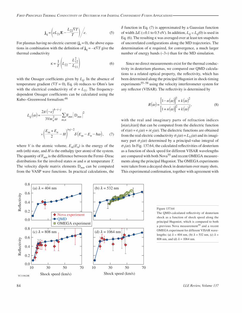
Since no direct measurements exist for the thermal conduc-tivity in deuterium plasmas, we compared our QMD calcula-tions to a related optical property, the reflectivity, which has been determined along the principal Hugoniot in shock-timing experiments55–58 using the velocity interferometer system for any reflector (VISAR). The reflectivity is determined by

,Rn k

n k

1

12 2

2 2-

~~ ~

~ ~=

+ +

+`

` `` `

jj jj j

99

CC

(8)

with the real and imaginary parts of refraction indices [n(~),k(~)] that can be computed from the dielectric function of e(~) = e1(~) + ie2(~). The dielectric functions are obtained from the real electric conductivity v1(~) = L11(~) and its imagi-nary part v2(~) determined by a principal-value integral of v1(~). In Fig. 137.64, the calculated reflectivities of deuterium as a function of shock speed for different VISAR wavelengths are compared with both Nova55 and recent OMEGA measure-ments along the principal Hugoniot. The OMEGA experiments were taken from a decayed shock in deuterium over many shots. This experimental confirmation, together with agreement with

TC11062JR

(a) m = 404 nm (b) m = 532 nm

0.2

0.4

0.6

0.8

0.0

Re�

ectiv

ity

0.2

0.4

0.6

0.8

0.0

Re�

ectiv

ity

3010 50 70

Shock speed (km/s) Shock speed (km/s)

3010 50 70

(c) m = 808 nm (d) m = 1064 nm

Nova experimentQMDOMEGA experiment

Figure 137.64The QMD-calculated reflectivity of deuterium shock as a function of shock speed along the principal Hugoniot, which is compared to both a previous Nova measurement55 and a recent OMEGA experiment for different VISAR wave-lengths: (a) m = 404 nm, (b) m = 532 nm, (c) m = 808 nm, and (d) m = 1064 nm.



other first-principle results,59 lends credence to the L11 coeffi-cients produced in this study and, in turn, to the other similarly calculated Onsager coefficients that determine l.

Thermal Conductivity of Deuterium for a Wide Range of Densities and Temperatures

The QMD calculations of deuterium thermal conductivity have been performed for a wide range of densities [t = 1.0 to 673.5 g/cm3], at temperatures varying from T = 5000 K to T = 8,000,000 K. For each density point, the lQMD calculations have been performed to the highest temperature approaching T - TF. (Tabulated results of lQMD are found in the Supple-mentary Material, p. 92.) To test the effects of lQMD on ICF implosions, we have fitted the lQMD results to the following function (in a similar format of lLILAC):

.

. .,

ln

m Z e

k T

Z

Z

20 2

1 0 24

0 095 0 24 1

/ / /

4

3 2 7 2 5 2

QMDe eff

B

eff

eff

QMD

#

##

#

lr

K

=

+

+

_

`_

i

ji

(9)

with the same Spitzer prefactor as used in lLILAC and Zeff = 1. The generalized QMD Coulomb logarithm has the following form:

.ln exp ln lnii

ii

i0

1

5

QMD a a b iK C= + +=

_ _ _i i i: D* 4/ (10)

This fifth-order polynomial function of coupling and degen-eracy parameters (C,i) has been fitted to the lQMD data using multivariable least-squares fitting. To make lQMD converge to lLILAC at the ideal plasma conditions (C % 1 and i & 1), we have added the high-temperature points of lLILAC into the data set for the global fitting. The resulting fitting parameters are:

.

.

.

.

.

.

.

.

.

.

.

E

E

E

E

E

E

E

0 74015

0 18146

6 39644 004

1 47954 003

1 23362 004

2 58107 005

0 86155

0 10570

6 75783 003

1 69007 004

3 49201 004

0

1

2

3

4

5

1

2

3

4

5

-

-

-

-

- -

- -

-

- -

- -

-

a

a

a

a

a

a

b

b

b

b

b

=

=

= +

= +

=

=

= +

=

=

=

= +

(11)

The fit results of (lnK)QMD are plotted in Figs. 137.65(a) and 137.65(b) as a function of ln(C) and ln(i), respectively. Overall,

Figure 137.65The generalized Coulomb logarithm, derived from QMD-calculated thermal conductivities for different densities and temperatures, is fitted with the poly-nomial function [Eq. (10)] of (a) the coupling parameter (C) and (b) the degeneracy parameter (i). The values of lnK at high temperatures [i.e., log(lnK) > 0] are converged to the standard LILAC values.

TC11063JR

0

4

–4

–8

log

(lnΛ

)

0 4–4

log (Γ)

(b)(a)

–8 0 4–4

log (i)

–8

QMDFitting



the global fitting with the above parameters gives only a small error of +5%.

Comparisons of lQMD with lLILAC are plotted in Figs. 137.66 and 137.67 for deuterium densities of t = 2.5, 10.0, 43.1, and 199.6 g/cm3. The green dashed lines represent the thermal con-

ductivity currently used in our hydrocode LILAC, while the blue solid triangles represent the QMD results. The red solid line is the QMD fit discussed above. We observe that lQMD is higher than lLILAC by a factor of 3 to 10 in the coupled and degenerate regimes (C > 1, i < 1). The QMD-fit line merges into lLILAC at a high-T regime (T > 10 TF), as expected.

TC11064JR

(a)

102

The

rmal

con

duct

ivity

l (

W/m

/K)

10–1 101

Temperature (eV)

100 102 103

(b)

Temperature (eV)

103

104

105

106

102

103

104

105

106

10–1 101100 102 103

107

LILACQMD �ttingQMD

TC11065JR

(a)

104

100 102

Temperature (eV)

101 103

(b)

Temperature (eV)

105

106

107

108

105

106

107

108

101 104102 103

109

The

rmal

con

duct

ivity

l (

W/m

/K)

LILACQMD �ttingQMD

Figure 137.66The thermal conductivities from first-principles QMD calculations, the QMD-fitting formula [Eq. (10)], and the hybrid model used in LILAC are plotted as a function of temperature for deuterium densities of (a) t = 2.5 g/cm2 and (b) t = 10.0 g/cm2.

Figure 137.67The thermal conductivities from first-principles QMD calculations, the QMD-fitting formula [Eq. (10)], and the hybrid model used in LILAC are plotted as a function of temperature for deuterium densities of (a) t = 43.1 g/cm2 and (b) t = 199.6 g/cm2.



Effects of lQMD on ICF ImplosionsTo test how the QMD-predicted thermal conductivity of DT

affects ICF implosions, we have incorporated the lQMD fit into our one-dimensional (1-D) radiation-hydrocode LILAC. The hydrodynamic simulations employed the flux-limited thermal conduction model60–63 with a flux limiter of f = 0.06. Two cryo-genic DT target implosions on OMEGA and three NIF direct-drive designs have been examined. These ICF implosions span a wide range of implosion velocities and adiabats. The adiabat (a) characterizes the plasma degeneracy degree of the imploding DT shell: the lower the adiabat, the more degenerate the DT plasma.

First, we show simulations of two cryogenic DT implosions on OMEGA in Figs. 137.68 and 137.69. A typical OMEGA cryogenic DT target has a diameter of +860 nm, which consists of a plastic ablator with a thickness of 8 to 11 nm and a layer of 45 to 65 nm of DT ice. In Fig. 137.68(a), the laser pulse has a relatively high first picket, which sets up the DT shell in a high adiabat of a - 4. The density and ion temperature profiles at the peak compression are plotted in Fig. 137.68(b). The blue dashed line represents the case of using standard lLILAC in the simulation, while the red solid line represents the lQMD simu-lation. Figure 137.68(b) shows that there is little change in the target performance for this high-adiabat implosion. In the end, the neutron yields are predicted to be 3.32 # 1014 (lLILAC) and 3.24 # 1014 (lQMD) for the two cases.

Predictions for the low-adiabat (a - 2.2) implosion are shown in Fig. 137.69. Figure 137.69(a) plots the laser pulse used for this OMEGA implosion. The in-flight plasma conditions are illustrated in Fig. 137.69(b) at t = 2.7 ns, just before stagnation, in which the mass density and electron temperature are drawn as a function of the target radius. Noticeable differences in electron-temperature profiles are seen for the two cases using lQMD and lLILAC; the peak density changed slightly when lQMD was used. These differences can affect the target performance at stagnation (t = 2.84 ns), as shown by Fig. 137.69(c). Finally, Fig. 137.69(d) indicates that the neutron yield is +6% lower in the lQMD simulation than for lLILAC. Table 137.VI summarizes the comparison of other quantities for the two simulations. The neutron-averaged compression tR and Ti are hardly changed, but the peak density and neutron yield vary by +6%.

Figure 137.68(a) The laser pulse shape used for a high-adiabat (a = 4) cryogenic DT implosion on OMEGA (the z = 868.8-nm capsule consists of 47 nm of DT ice with an 8.4-nm-thick plastic ablator); (b) comparisons of the density and ion-temperature profiles at peak compression for the two hydrodynamic runs using lLILAC (blue dashed lines) and lQMD (red solid lines), respectively. Very little difference is seen in target performance for the two thermal-conductivity models used for such a high-adiabat implosion. Green arrows indicate the vertical axis that applies to each curve.

TC11066JR

(a)

10

Las

er in

tens

ity (

W/c

m2 )

(×

1014

)

0 1

Time (ns)

2 0 2010 30 40

150

100

200

50

0

Den

sity

(g/

cm3 )

Ti (

keV

)

(b)

Radius (nm)

8

6

4

2

0 0

4

6

2

lLILAClQMD

Table 137.VI: Comparison of an OMEGA implosion (a - 2.2) predicted using lLILAC versus lQMD.

lLILAC lQMD

GtRHn 298 mg/cm2 296 mg/cm2

GTiHn 4.66 keV 4.64 keV

GPHn 197 Gbar 194 Gbar

GtHpeak 380.8 g/cm3 361.7 g/cm3

Yield 5.34 # 1014 5.05 # 1014



Figure 137.69(a) The laser pulse shape used for a low-adiabat (a = 2.2) cryogenic DT implosion on OMEGA (the z = 860.6-nm capsule consists of 49 nm of DT ice with an 8.3-nm-thick plastic ablator). [(b),(c)] Comparisons of the density and temperature profiles at the beginning of the deceleration phase and at peak compression, respectively, for the two hydrodynamic simulations using lLILAC (blue dashed lines) and lQMD (red solid lines). (d) The neutron yields as a function of time are plotted for the two cases. A modest variation (+6%) in target performance is seen in such low-adiabat OMEGA implosions, when lQMD is compared to the hybrid LILAC model.

TC11067JR

(a)

2

6

8

10

0

4

8

12

16

0

Las

er in

tens

ity (

W/c

m2 )

(×

1014

)

4

1 2 3

Time (ns) Radius (nm)

0 40 60 80 100

Den

sity

(g/

cm3 )

40

60

80

20

Te

(eV

)

(d)

100

200

300

400

0

4.5

5.0

5.5

6.0

4.0

Den

sity

(g/

cm3 )

10 20 30

Radius (nm) Time (ns)

0 2.6 2.8 3.0

Neu

tron

yie

ld (

×10

14)

6

4

2

0

Ti (

keV

)

lLILAClQMD

(c)(c)

(b)(b)

Next we discuss the lQMD effects on three different direct-drive–ignition designs for the NIF. These NIF designs have slightly different target sizes varying from z = 3294 nm to z = 3460 nm. The thickness of the DT-ice layer changes from d = 125 nm to d = 220 nm; all targets have a plastic ablator at somewhat different thicknesses of 22 to 30 nm. We discuss the lQMD effects on the performance of three NIF designs from a mid-adiabat (a = 3.2) implosion to a very low adiabat (a = 1.7) design. Figure 137.70 shows first the mid-adiabat (a = 3.2) design: (a) the triple-picket pulse shape (total energy of 1.5 MJ) and (b) the density and ion-temperature profiles at the bang time (t = 13.78 ns, i.e., the time for peak neutron production). Similar to what was seen in Fig. 137.68, only small differences between lQMD and lLILAC simulations are observed for this mid-adiabat NIF design. The comparison of target performance is summarized in Table 137.VII, in which the differences in neutron-averaged tR, Ti, pressure GPHn, hot-spot radius Rhs, hot-spot convergence ratio Chs, neutron yield, and gain are all within +2%.

Table 137.VII: Comparison of a mid-adiabat (a = 3.2) NIF design simulated with lLILAC versus lQMD.

lLILAC lQMD

GtRHn 0.654 g/cm2 0.655 g/cm2




Rhs 91.4 nm 91.3 nm

Chs 18.9 18.9

Yield 6.45 # 1018 6.33 # 1018

Gain 12.1 11.8

Figure 137.71 illustrates the simulation results for a slightly lower adiabat (a - 2.5), high-convergence NIF design. Similar to Fig. 137.69 for the a = 2.2 OMEGA implosion, Figs. 137.71(a)–137.71(d) plot (a) the pulse shape (total energy of 1.6 MJ),



TC11068JR

(a)8

6

4

2

0

Las

er in

tens

ity (

W/c

m2 )

(×

1014

)

Ti (

keV

)

0 6

Time (ns)

3 9 12 0 100 100 20050

300

200

100

0

15

10

20

5

0

Den

sity

(g/

cm3 )

(b)

Radius (nm)

lLILAClQMD

TC11069JR

(a)

2

6

8

0

4

8

12

16

0

Las

er in

tens

ity(W

/cm

2 ) (

×10

14) 10

4

2 4 6 8 10Time (ns) Radius (nm)

0 220 260 300

Den

sity

(g/

cm3 )

40

60

80

Te

(eV

)(d)

100

200

300

0

6.0

6.5

7.0

5.5

Den

sity

(g/

cm3 ) 400

500

50 100 150


0 9 10 11

Neu

tron

yie

ld (

×10

18)30

20

10

0

Ti (

keV

)

lLILAClQMD

(b)(b)

(c)(c)

Figure 137.70Similar to Fig. 137.68 but for a NIF-scale implosion: (a) The laser pulse shape for a mid-adiabat (a = 3.2), 1.5-MJ direct-drive NIF design (the z = 3460-nm capsule consists of 220 nm of DT ice with a 30-nm-thick plastic ablator); (b) comparisons of the density and ion-temperature profiles at the peak compression for the two hydrodynamic runs using lLILAC (blue dashed lines) and lQMD (red solid lines), respectively. The effects of using different l are small for such mid-adiabat designs.

Figure 137.71Tests on a high-implosion-velocity NIF design: (a) The laser pulse shape (a = 2.5) has a total energy of 1.6 MJ (the z = 3294-nm capsule consists of 125 nm of DT ice with a 22-nm-thick plastic ablator). Panels (b) and (c) compare the density and temperature profiles at the beginning of the deceleration phase and at peak compression, respectively, for the two hydrodynamic simulations using lLILAC (blue dashed lines) and lQMD (red solid lines). The neutron yields as a function of time are plotted in panel (d) for the two cases. The use of lQMD modestly changes the 1-D prediction of implosion performance (+6%).



(b) the in-flight density and electron-temperature profiles at t = 8.6 ns, (c) the bang-time density and ion-temperature profiles at t = 8.91 ns, and (d) the final neutron yield. Again, some slight differences in the electron temperature at the back surface of the shell can be seen in Fig. 137.71(b). The observables predicted by the two hydrodynamic simulations using lQMD in contrast to lLILAC are summarized in Table 137.VIII. Overall, a level of +6% increase in target performance is seen in the lQMD simula-tion when compared to the standard lLILAC case.

Table 137.VIII: Comparison of a low-adiabat (a = 2.5) NIF design simulated with lLILAC versus lQMD.

lLILAC lQMD

GtRHn 0.646 g/cm2 0.661 g/cm2




Rhs 56.2 nm 53.8 nm

Chs 29.3 30.6

Yield 6.3 # 1018 6.7 # 1018

Gain 11.1 11.7

We further analyze the implosion dynamics of the NIF design shown in Fig. 137.71. The noticeable t/Te differences at the back of the shell illustrated by Fig. 137.71(b) must come from the different shock dynamics in early stages of the implosion. To further explore the differences, in Fig. 137.72 we have plotted the DT plasma conditions at the shock transit stage. In Fig. 137.72(a), the density and temperature profiles are displayed for a snapshot at t = 4.0 ns. To clearly see the differences, we have plotted these profiles as a function of the simulation Lagrangian cell number. At this snapshot, the first shock [dashed circle in Fig. 137.63(a)] has propagated to near the back surface (at the 150th cell) of the DT ice layer. An interesting difference between two simulations can be clearly seen at the first shock front (near the 165th cell), in which the temperature front (at the 175th cell) predicted by the lLILAC simulation does not follow the density front of the shock. This occurs because the standard lLILAC significantly underesti-mates the thermal conductivity by an order of magnitude, for the shocked-DT plasma condition of tDT - 1 g/cm2 and Te - 1 to 2 eV. The reduced thermal conductivity in lLILAC decreases the heat flow behind the shock front. On the contrary, the lQMD simulation (red solid lines) indicates the same shock-front loca-tion for both density and temperature, as expected. Differences in both density and temperature are also seen after the second

TC11070JR

(a)

0.4

0.8

1.2

0.0

Den

sity

(g/

cm3 )

0.4

0.8

1.2

0.0

Den

sity

(g/

cm3 )

Cell number

150 200 250 300

lLILAClQMD

150 250200

4

2

6

8

0

Te

(eV

)

4

2

6

8

0

Te

(eV

)

(b)

Cell number

Figure 137.72The predicted shock conditions during the shock transit stage in the DT ice, for the NIF design plotted in Fig. 137.71. The density and electron temperature are plotted as a function of the Lagrangian cell numbers for times at (a) t = 4.0 ns and (b) t = 4.8 ns. Again, the two cases of using lLILAC (blue dashed lines) and lQMD (red solid lines) are compared. The dashed circle highlights the first shock.

shock [near the 260th cell shown in Fig. 137.72(a)]. The lLILAC simulation predicts more “artificial” fluctuations in density and temperature after the second shock. Figure 137.72(b) shows another snapshot at t = 4.8 ns, when the first shock breaks out at the back of the DT ice layer into the DT gas. A large difference in electron-temperature profile is observed for the two simula-tions: the instant heat conduction in the lQMD case results in



the immediate heating up of the releasing back surface, which is in contrast to the delayed heating in the lLILAC simulation. These different shock dynamics at the early stage of implosion cause the observable density–temperature variations late in the implosion, plotted in Fig. 137.71(b). This is the major contribu-tion responsible for the final difference in target performance, which is discussed below.

Finally, the very low adiabat (a - 1.7) NIF design is exam-ined in Fig. 137.73 and Table 137.IX. The implosion is designed to be driven by a 1.2-MJ pulse shape shown in Fig. 137.73(a), which has a ramping and low-intensity main pulse to avoid possible preheat from two-plasmon-decay–induced hot elec-trons.64,65 The implosion velocity for this design is about 3.3 # 107 cm/s. Since the adiabat is so low that the DT-plasma conditions for the in-flight shell lie deeply within the more-degenerate and coupled regime, where lQMD is much higher than lLILAC, the effects of using lQMD are dramatically increased when compared to the higher-adiabat implosions discussed above. From Table 137.IX and Fig. 137.73, an +20% variation in target performance (yield and gain) is observed in

TC11071JR

(a)

2

6

8

0

2

4

8

10

0

Las

er in

tens

ity(W

/cm

2 ) (

×10

14)

64

5 10 150 350 400 450 500 550

Den

sity

(g/

cm3 )

20

30

40

50

10

(d)

100

200

300

0

7

8

9

5

Den

sity

(g/

cm3 )

6

400

500

50 100 150 2000 14 15 1613 17

Neu

tron

yie

ld (

×10

18)20

15

10

5

0

Ti (

keV

)

(c)(c)

(b)(b)

Time (ns) Radius (nm)


Te

(eV

)

lLILAClQMD

Figure 137.73Similar to Fig. 137.71 but for a relatively lower adiabat (a = 1.7) and lower implosion velocity (Vimp = 3.3 # 107 cm/s) NIF design: (a) The laser pulse shape has a total energy of 1.2 MJ and the z = 3420-nm capsule consists of 180 nm of DT ice with a 30-nm-thick plastic ablator. [(b),(c)] Comparison of the density and temperature profiles at the beginning of the deceleration phase and at the peak compression, respectively. (d) Comparison of the neutron yields for the two cases, which shows an ~20% variation in the 1-D predictions of target performance using lLILAC and lQMD.

Table 137.IX: Comparison of a very low adiabat (a = 1.7) NIF design simulated with lLILAC versus lQMD.

lLILAC lQMD

GtRHn 0.679 g/cm2 0.69 g/cm2




Rhs 80.9 nm 79.3 nm

Chs 21.1 21.6

Yield 7.07 # 1018 8.41 # 1018

Gain 16.6 19.7

the predictions of the two cases. Figure 137.73(b) shows that the simulation using lQMD predicts a lower electron-temperature profile for the back of the shell (R - 420 nm). This results in a larger peak density of the shell and higher Ti at the bang time for the lQMD case, illustrated by Fig. 137.73(c), thereby leading to more neutron yields and gain.



To test the conventional speculation that lQMD affects mainly the hot-spot formation, we performed a “hybrid” simu-lation for this design by switching lQMD to the standard lLILAC during the target deceleration phase and burn (t > 13.6 ns). This hybrid simulation gives a total neutron yield of 9.29 # 1018

and a gain of 21.8. Comparing with the full lQMD simulation results (Y = 8.41 # 1018 and G = 19.7), the variation is modest with respect to the change from the full lLILAC simulation to the full lQMD case. This indicates that the major part of the lQMD effects on target performance comes from the shock dynamics during the early stage of the implosion, although the use of lQMD moderately decreases the target performance during the hot-spot formation.

SummaryFor inertial confinement fusion applications, we have per-

formed first-principles calculations of deuterium thermal con-ductivity in a wide range of densities and temperatures, using the quantum molecular dynamics method. For the density and temperature conditions in an imploding DT shell, the QMD-calculated thermal conductivity lQMD is higher by a factor of 3 to 10 than the hybrid Spitzer–Lee–More model lLILAC currently adopted in our hydrocodes. To test its effects on ICF implosions, we have fitted lQMD to a fifth-order polynomial function of C and i and incorporated this fit into our hydro-codes. The hydrodynamic simulations of both OMEGA cryo-genic DT implosions and direct-drive NIF designs have been performed using lQMD. Compared with the standard simulation results using lLILAC, we found the ICF implosion performance predicted by lQMD could vary by as much as +20%. The lower the adiabat of the DT shell, the more the effects of lQMD are observed. Analyses of the implosion dynamics have identi-fied that the shock-dynamic differences at an early stage of the implosion, predicted differently by lQMD versus lLILAC, predominantly contribute to the final variations of implosion performance (neutron yield and target gain). This is in con-trast to the previous speculation that lQMD might affect ICF mainly during the hot-spot formation. The thermal conductivi-ties of deuterium reported here, together with the established FPEOS tables11,45 and opacity tables (future work) from such first-principles calculations, could provide complete physical information of fusion fuel at high-energy-density conditions for accurate ICF hydrodynamic simulations. The same strategy also applies for building self-consistent tables of ICF-relevant ablator materials. These efforts could increase the predictive capability of hydrodynamic modeling of ICF implosions.

Supplementary Material

Table 137.X: The thermal-conductivity (lQMD) table of deuterium for a wide range of densities.

Temperature T (K) lQMD (W/m/K)

t = 1.000 g/cm3 (rS = 1.753 bohr)

5,000 59.87!4.93

10,000 127.3!10.3

15,625 202.1!13.2

31,250 451.6!18.7

62,500 1199.6!49.6

95,250 2227.5!90.3

125,000 3281.4!139.0

181,825 6041.6!144.3

250,000 10491.2!203.1

t = 1.963 g/cm3 (rS = 1.4 bohr)

5,000 239.77!21.7

10,000 374.07!34.46

15,625 492.57!43.67

31,250 (1.00!0.04) # 103

62,500 (2.17!0.09) # 103

95,250 (3.68!0.21) # 103

125,000 (5.17!0.25) # 103

181,825 (8.41!0.37) # 103

250,000 (1.30!0.02) # 104

400,000 (2.32!0.02) # 104

t = 2.452 g/cm3 (rS = 1.3 bohr)

5,000 345.5!39.5

10,000 499.2!47.6

15,625 676.5!41.6

31,250 (1.21!0.08) # 103

62,500 (2.74!0.11) # 103

95,250 (4.38!0.18) # 103

125,000 (6.26!0.29) # 103

181,825 (1.00!0.04) # 104

250,000 (1.53!0.04) # 104

400,000 (2.79!0.05) # 104



Table 137.X (continued).


t = 3.118 g/cm3 (rS = 1.2 bohr)

5,000 472.5!54.6

10,000 745.7!76.2

15,625 953.7!72.2

31,250 (1.61!0.10) # 103

62,500 (3.55!0.20) # 103

95,250 (5.53!0.25) # 103

125,000 (7.61!0.30) # 103

181,825 (1.24!0.04) # 104

250,000 (1.85!0.05) # 104

400,000 (3.47!0.08) # 104

t = 4.048 g/cm3 (rS = 1.1 bohr)

5,000 778.8!83.3

10,000 (1.03!0.08) # 103

15,625 (1.36!0.12) # 103

31,250 (2.12!0.05) # 103

62,500 (4.48!0.22) # 103

95,250 (7.17!0.28) # 103

125,000 (9.75!0.52) # 103

181,825 (1.51!0.06) # 104

250,000 (2.32!0.08) # 104

400,000 (4.36!0.12) # 104

t = 5.388 g/cm3 (rS = 1.0 bohr)

5,000 (1.19!0.17) # 103

10,000 (1.41!0.15) # 103

15,625 (1.84!0.27) # 103

31,250 (2.76!0.32) # 103

62,500 (5.60!0.25) # 103

95,250 (9.33!0.42) # 103

125,000 (1.27!0.06) # 104

181,825 (2.01!0.06) # 104

250,000 (2.91!0.11) # 104

400,000 (5.53!0.17) # 104

500,000 (9.48!0.13) # 104



t = 7.391 g/cm3 (rS = 0.9 bohr)

5,000 (2.00!0.37) # 103

10,000 (2.24!0.21) # 103

15,625 (2.67!0.28) # 103

31,250 (4.14!0.33) # 103

62,500 (7.59!0.59) # 103

95,250 (1.30!0.07) # 104

125,000 (1.75!0.10) # 104

181,825 (2.61!0.08) # 104

250,000 (3.80!0.17) # 104

400,000 (6.94!0.23) # 104

500,000 (9.52!0.33) # 104

t = 10.000 g/cm3 (rS = 0.814 bohr)

5,000 (3.01!0.48) # 103

10,000 (3.34!0.55) # 103

15,625 (3.77!0.43) # 103

31,250 (5.74!0.46) # 103

62,500 (9.65!0.69) # 103

95,250 (1.66!0.12) # 104

125,000 (2.32!0.13) # 104

181,825 (3.40!0.19) # 104

250,000 (4.78!0.29) # 104

400,000 (8.37!0.32) # 104

500,000 (1.24!0.04) # 105

t = 15.709 g/cm3 (rS = 0.8 bohr)

10,000 (7.29!0.70) # 103

15,625 (7.57!0.80) # 103

31,250 (1.20!0.09) # 104

62,500 (1.99!0.11) # 104

95,250 (2.78!0.17) # 104

125,000 (3.50!0.17) # 104

181,825 (5.24!0.21) # 104

250,000 (7.50!0.33) # 104

400,000 (1.34!0.05) # 105

500,000 (1.80!0.04) # 105

1,000,000 (3.79!0.11) # 105





t = 24.945 g/cm3 (rS = 0.6 bohr)

15,625 (1.49!0.15) # 104

31,250 (1.71!0.13) # 104

62,500 (3.18!0.21) # 104

95,250 (4.24!0.27) # 104

125,000 (5.31!0.27) # 104

181,825 (7.06!0.49) # 104

250,000 (9.95!0.35) # 104

400,000 (1.68!0.07) # 105

500,000 (2.19!0.11) # 105

1000,000 (5.63!0.21) # 105

t = 43.105 g/cm3 (rS = 0.5 bohr)

31,250 (3.09!0.33) # 104

62,500 (5.14!0.40) # 104

95,250 (7.36!0.78) # 104

125,000 (8.82!0.64) # 104

181,825 (1.17!0.08) # 105

250,000 (1.44!0.15) # 105

400,000 (2.46!0.08) # 105

500,000 (3.14!0.24) # 105

1,000,000 (7.62!0.28) # 105

t = 84.190 g/cm3 (rS = 0.4 bohr)

31,250 (7.72!0.98) # 104

62,500 (7.52!0.64) # 104

95,250 (1.21!0.15) # 105

125,000 (1.64!0.17) # 105

181,825 (2.03!0.27) # 105

250,000 (2.65!0.33) # 105

400,000 (3.74!0.35) # 105

500,000 (4.66!0.24) # 105

1,000,000 (1.15!0.06) # 106

2,000,000 (3.12!0.05) # 106



t = 199.561 g/cm3 (rS = 0.3 bohr)

125,000 (4.93!0.21) # 105

181,825 (6.18!0.24) # 105

250,000 (8.19!0.20) # 105

400,000 (1.25!0.05) # 106

500,000 (1.52!0.06) # 106

1,000,000 (2.86!0.09) # 106

2,000,000 (6.38!0.09) # 106

4,000,000 (1.57!0.10) # 107

t = 673.518 g/cm3 (rS = 0.2 bohr)

250,000 (2.43!0.17) # 106

400,000 (3.18!0.24) # 106

500,000 (3.76!0.26) # 106

1,000,000 (7.34!0.35) # 106

2,000,000 (1.44!0.07) # 107

4,000,000 (3.33!0.06) # 107

8,000,000 (8.92!0.08) # 107

ACKNOWLEDGMENTThis material is based on work supported by the Department of

Energy National Nuclear Security Administration under Award Number DE-NA0001944, the University of Rochester, and the New York State Energy Research and Development Authority. This work was also supported by Scientific Campaign 10 at the Los Alamos National Laboratory, operated by Los Alamos National Security, LLC for the National Nuclear Security Admin-istration of the U.S. Department of Energy under Contract No. DE-AC52-06NA25396. The support of DOE does not constitute an endorsement by DOE of the views expressed in this article. SXH acknowledges the advice from Prof. G. Kresse on the Coulombic potential for high-density VASP simulations.

REFERENCES

1. J. Nuckolls et al., Nature 239, 139 (1972); S. Atzeni and J. Meyer-ter-Vehn, The Physics of Inertial Fusion: Beam Plasma Interaction, Hydrodynam-ics, Hot Dense Matter, International Series of Monographs on Physics (Clarendon Press, Oxford, 2004).

2. J. D. Lindl, Phys. Plasmas 2, 3933 (1995).

3. C. Cherfils-Clérouin et al., J. Phys.: Conf. Ser. 244, 022009 (2010).



4. R. L. McCrory, R. Betti, T. R. Boehly, D. T. Casey, T. J. B. Collins, R. S. Craxton, J. A. Delettrez, D. H. Edgell, R. Epstein, J.A. Frenje, D. H. Froula, M. Gatu-Johnson, V. Yu. Glebov, V. N. Goncharov, D. R. Harding, M. Hohenberger, S. X. Hu, I. V. Igumenshchev, T. J. Kessler, J. P. Knauer, C.K. Li, J. A. Marozas, F. J. Marshall, P. W. McKenty, D. D. Meyerhofer, D. T. Michel, J. F. Myatt, P. M. Nilson, S. J. Padalino, R.D. Petrasso, P. B. Radha, S. P. Regan, T. C. Sangster, F. H. Séguin, W. Seka, R. W. Short, A. Shvydky, S. Skupsky, J. M. Soures, C. Stoeckl, W. Theobald, B. Yaakobi, and J. D. Zuegel, Nucl. Fusion 53, 113021 (2013).

5. D. D. Meyerhofer, R. L. McCrory, R. Betti, T. R. Boehly, D. T. Casey, T. J. B. Collins, R. S. Craxton, J. A. Delettrez, D. H. Edgell, R. Epstein, K. A. Fletcher, J. A. Frenje, Y. Yu. Glebov, V. N. Goncharov, D. R. Harding, S. X. Hu, I. V. Igumenshchev, J. P. Knauer, C. K. Li, J. A. Marozas, F. J. Marshall, P. W. McKenty, P. M. Nilson, S. P. Padalino, R. D. Petrasso, P. B. Radha, S. P. Regan, T. C. Sangster, F. H. Séguin, W. Seka, R. W. Short, D. Shvarts, S. Skupsky, J. M. Soures, C. Stoeckl, W. Theobald, and B. Yaakobi, Nucl. Fusion 51, 053010 (2011).

6. V. N. Goncharov, T. C. Sangster, T. R. Boehly, S. X. Hu, I. V. Igumenshchev, F. J. Marshall, R. L. McCrory, D. D. Meyerhofer, P. B. Radha, W. Seka, S. Skupsky, C. Stoeckl, D. T. Casey, J. A. Frenje, and R. D. Petrasso, Phys. Rev. Lett. 104, 165001 (2010).

7. M. C. Herrmann, M. Tabak, and J. D. Lindl, Nucl. Fusion 41, 99 (2001).

8. C. D. Zhou and R. Betti, Phys. Plasmas 15, 102707 (2008).

9. S. X. Hu, V. A. Smalyuk, V. N. Goncharov, J. P. Knauer, P. B. Radha, I. V. Igumenshchev, J. A. Marozas, C. Stoeckl, B. Yaakobi, D. Shvarts, T. C. Sangster, P. W. McKenty, D. D. Meyerhofer, S. Skupsky, and R. L. McCrory, Phys. Rev. Lett. 100, 185003 (2008).

10. J. Clérouin and J.-F. Dufrêche, Phys. Rev. E 64, 066406 (2001); L. Caillabet, S. Mazevet, and P. Loubeyre, Phys. Rev. B 83, 094101 (2011).

11. S. X. Hu, B. Militzer, V. N. Goncharov, and S. Skupsky, Phys. Rev. B 84, 224109 (2011).

12. M. A. Morales et al., High Energy Density Phys. 8, 5 (2012).

13. S. Hamel, L. X. Benedict, P. M. Celliers, M. A. Barrios, T. R. Boehly, G. W. Collins, T. Döppner, J. H. Eggert, D. R. Farley, D. G. Hicks, J. L. Kline, A. Lazicki, S. LePape, A. J. Mackinnon, J. D. Moody, H. F. Robey, E. Schwegler, and P. A. Sterne, Phys. Rev. B 86, 094113 (2012); P. Loubeyre, S. Brygoo, J. Eggert, P. M. Celliers, D. K. Spaulding, J. R. Rygg, T. R. Boehly, G. W. Collins, and R. Jeanloz, Phys. Rev. B 86, 144115 (2012).

14. J. Vorberger, D. O. Gericke, and W. D. Kraeft, High Energy Density Phys. 9, 448 (2013).

15. C. Wang and P. Zhang, Phys. Plasmas 20, 092703 (2013).

16. V. V. Karasiev et al., Phys. Rev. B 88, 161108 (2013).

17. B. Militzer and D. M. Ceperley, Phys. Rev. Lett. 85, 1890 (2000); B. Militzer et al., Phys. Rev. Lett. 87, 275502 (2001).

18. J. M. McMahon et al., Rev. Mod. Phys. 84, 1607 (2012).

19. L. Collins et al., Phys. Rev. E 52, 6202 (1995).

20. H. Brysk, P. M. Campbell, and P. Hammerling, Plasma Phys. 17, 473 (1975).

21. L. Spitzer, Jr. and R. Härm, Phys. Rev. 89, 977 (1953).

22. J. Daligault and G. Dimonte, Phys. Rev. E 79, 056403 (2009).

23. L. X. Benedict et al., Phys. Rev. Lett. 102, 205004 (2009).

24. B. Xu and S. X. Hu, Phys. Rev. E 84, 016408 (2011).

25. L. X. Benedict et al., Phys. Rev. E 86, 046406 (2012).

26. C. Blancard, J. Clérouin, and G. Faussurier, High Energy Density Phys. 9, 247 (2013).

27. W. B. Hubbard, Astrophys. J. 146, 858 (1966).

28. Y. T. Lee and R. M. More, Phys. Fluids 27, 1273 (1984).

29. S. Ichimaru and S. Tanaka, Phys. Rev. A 32, 1790 (1985); H. Kitamura and S. Ichimaru, Phys. Rev. E 51, 6004 (1995).

30. D. A. Liberman, Phys. Rev. B 20, 4981 (1979).

31. B. Wilson et al., J. Quant. Spectrosc. Radiat. Transf. 99, 658 (2006).

32. G. Faussurier et al., Phys. Plasmas 17, 052707 (2010); J. Clérouin et al., Phys. Rev. E 82, 046402 (2010).

33. J. G. Clérouin and S. Bernard, Phys. Rev. E 56, 3534 (1997).

34. L. A. Collins et al., Phys. Rev. B 63, 184110 (2001).

35. M. P. Desjarlais, Phys. Rev. B 68, 064204 (2003).

36. S. A. Bonev, B. Militzer, and G. Galli, Phys. Rev. B 69, 014101 (2004).

37. J. D. Kress et al., Phys. Rev. E 82, 036404 (2010).

38. V. Recoules et al., Phys. Rev. Lett. 102, 075002 (2009).

39. F. Lambert et al., Phys. Plasmas 18, 056306 (2011).

40. D. E. Hanson et al., Phys. Plasmas 18, 082704 (2011).

41. B. Holst, M. French, and R. Redmer, Phys. Rev. B 83, 235120 (2011).

42. C. E. Starrett et al., Phys. Plasmas 19, 102709 (2012).

43. C. Wang et al., Phys. Rev. E 88, 013106 (2013).

44. For details of the ABINIT code, please refer to http://www.abinit.org/.

45. S. X. Hu, B. Militzer, V. N. Goncharov, and S. Skupsky, Phys. Rev. Lett. 104, 235003 (2010).



46. R. Kubo, J. Phys. Soc. Jpn. 12, 570 (1957); D. A. Greenwood, Proc. Phys. Soc. Lond. 71, 585 (1958).

47. J. Delettrez, R. Epstein, M. C. Richardson, P. A. Jaanimagi, and B. L. Henke, Phys. Rev. A 36, 3926 (1987).

48. I. Kwon, J. D. Kress, and L. A. Collins, Phys. Rev. B 50, 9118 (1994).

49. M. P. Desjarlais, J. D. Kress, and L. A. Collins, Phys. Rev. E 66, 025401 (2002).

50. B. Holst, R. Redmer, and M. P. Desjarlais, Phys. Rev. B 77, 184201 (2008).

51. G. Kresse and J. Hafner, Phys. Rev. B 47, 558 (1993).

52. G. Kresse and J. Hafner, Phys. Rev. B 49, 14,251 (1994); G. Kresse and J. Furthmüller, Phys. Rev. B 54, 11,169 (1996).

53. G. Kresse and D. Joubert, Phys. Rev. B 59, 1758 (1999).

54. G. Kresse, University of Vienna, private communication (2013).

55. P. M. Celliers et al., Phys. Rev. Lett. 84, 5564 (2000).

56. T. R. Boehly, D. H. Munro, P. M. Celliers, R. E. Olson, D. G. Hicks, V. N. Goncharov, G. W. Collins, H. F. Robey, S. X. Hu, J. A. Marozas, T. C. Sangster, O. L. Landen, and D. D. Meyerhofer, Phys. Plasmas 16, 056302 (2009).

57. T. R. Boehly, V. N. Goncharov, W. Seka, S. X. Hu, J. A. Marozas, D. D. Meyerhofer, P. M. Celliers, D. G. Hicks, M. A. Barrios, D. Fratanduono, and G. W. Collins, Phys. Plasmas 18, 092706 (2011).

58. T. R. Boehly, V. N. Goncharov, W. Seka, M. A. Barrios, P. M. Celliers, D. G. Hicks, G. W. Collins, S. X. Hu, J. A. Marozas, and D. D. Meyerhofer, Phys. Rev. Lett. 106, 195005 (2011).

59. L. A. Collins, J. D. Kress, and D. E. Hanson, Phys. Rev. B 85, 233101 (2012).

60. R. C. Malone, R. L. McCrory, and R. L. Morse, Phys. Rev. Lett. 34, 721 (1975).

61. S. X. Hu, V. Smalyuk, V. N. Goncharov, S. Skupsky, T. C. Sangster, D. D. Meyerhofer, and D. Shvarts, Phys. Rev. Lett. 101, 055002 (2008).

62. S. X. Hu, P. B. Radha, J. A. Marozas, R. Betti, T. J. B. Collins, R. S. Craxton, J. A. Delettrez, D. H. Edgell, R. Epstein, V. N. Goncharov, I. V. Igumenshchev, F. J. Marshall, R. L. McCrory, D. D. Meyerhofer, S. P. Regan, T. C. Sangster, S. Skupsky, V. A. Smalyuk, Y. Elbaz, and D. Shvarts, Phys. Plasmas 16, 112706 (2009).

63. S. X. Hu, V. N. Goncharov, P. B. Radha, J. A. Marozas, S. Skupsky, T. R. Boehly, T. C. Sangster, D. D. Meyerhofer, and R. L. McCrory, Phys. Plasmas 17, 102706 (2010).

64. D. H. Froula, B. Yaakobi, S. X. Hu, P.-Y. Chang, R. S. Craxton, D. H. Edgell, R. Follett, D. T. Michel, J. F. Myatt, W. Seka, R. W. Short, A. Solodov, and C. Stoeckl, Phys. Rev. Lett. 108, 165003 (2012).

65. S. X. Hu, D. T. Michel, D. H. Edgell, D. H. Froula, R. K. Follett, V. N. Goncharov, J. F. Myatt, S. Skupsky, and B. Yaakobi, Phys. Plasmas 20, 032704 (2013).

first-principles thermal conductivity of deuterium for

Documents