WP/16/230

Fiscal Discipline and Exchange Rates: Does Politics Matter?

by Joao Tovar Jalles, Carlos Mulas-Granados, and José Tavares

2

© 2016 International Monetary Fund WP/16/230

IMF Working Paper

Fiscal Affairs Department

Fiscal Discipline and Exchange Rates: Does Politics Matter?1

Prepared by Joao Tovar Jalles, Carlos Mulas-Granados, and José Tavares

Authorized for distribution by Catherine Pattillo

November 2016

Abstract

JEL Classification Numbers: H11, H62, H63

Keywords: Fiscal discipline; Deficit; Political Economy; Exchange Rates

Author’s E-Mail Address: JJalles@imf.org; CMulasGranados@imf.org; JTavares@novasbe.pt

1 We are grateful to Vitor Gaspar, Sanjeev Gupta and Ben Clements for useful comments and suggestions. Participants of the FAD Seminar Series also contributed with valuable discussions. We also thank Jaime Marques Pereira, Michela Schena and Carolina Correa Caro for excellent research assistance. The opinions expressed herein are those of the authors and do not necessarily reflect those of the authors’ employers. J. Jalles and C. Mulas-Granados are with the International Monetary Fund. J. Tavares is with the New University of Lisbon.

This Working Paper should not be reported as representing the views of the IMF. The views expressed in this Working Paper are those of the author(s) and do not necessarily represent those of the IMF or IMF policy. Working Papers describe research in progress by the author(s) and are published to elicit comments and to further debate.

We look at the effect of exchange rate regimes on fiscal discipline, taking into account the effect of underlying political conditions. We present a model where strong politics (defined as policymakers facing longer political horizon and higher cohesion) are associated with better fiscal performance, but fixed exchange rates may revert this result and lead to less fiscal discipline. We confirm these hypotheses through regression analysis performed on a panel sample covering 79 countries from 1975 to 2012. Our empirical results also show that the positive effect of strong politics on fiscal discipline is not enough to counter the negative impact of being at/moving to fixed exchange rates. Finally, we use the synthetic control method to illustrate how the transition from flexible to fully fixed exchange rate under the Euro impacted negatively fiscal discipline in European countries. Our results are robust to a number of important sensitivity checks, including different estimators, alternative proxies for fiscal discipline, and sub-sample analysis.

3

Contents Page

I. Introduction _____________________________________________________________________________________ 4 

II. Literature Review: Exchange Rate Regimes and Fiscal Discipline _______________________________ 6 

III. Theoretical Framework _________________________________________________________________________ 8 

IV. Empirical Analysis _____________________________________________________________________________ 12 

V. Robustness Checks ____________________________________________________________________________ 17 

VI. Case Study: Fiscal Discipline and Fixed Exchange Rates in the Eurozone _____________________ 22 

VII. Conclusion ___________________________________________________________________________________ 25 

References ________________________________________________________________________________________ 29  FIGURES 1. Political Horizon and Indebtedness __________________________________________________________________ 11 2. Political Cohesion and Indebtedness ________________________________________________________________ 11 3. Primary Balance, Exchange Rates, and Political Conditions __________________________________________ 14 4. Synthetic Control Analysis, Euro-11 _________________________________________________________________ 24  TABLES 1. Summary of Political Composite Variables and Descriptive Statistics _______________________________ 13 2. Factor Loadings and Uniqueness ____________________________________________________________________ 14 3. Baseline, Fixed Effects Regressions __________________________________________________________________ 16 4. Interaction Terms, Fixed Effects Regressions ________________________________________________________ 17 5. Sensitivity to Alternative Estimators _________________________________________________________________ 18 6. Endogeneity: Instrumental Variables ________________________________________________________________ 19 7. Discretionary Fiscal Consolidations as Proxy for Fiscal Discipline: Logit Estimations ________________ 21 8. Robustness to Alternative Definition of ER Regime _________________________________________________ 22  APPENDICES 1. Robustness __________________________________________________________________________________________ 26 2. Synthetic Control Methodology _____________________________________________________________________ 27  APPENDIX TABLES A1. Robustness to Alternative Measures of Fiscal Discipline ___________________________________________ 26 

4

I. INTRODUCTION

The issue of what type of exchange rate regime is better for fiscal discipline has a long tradition in macroeconomics. Traditionally, the view that fixed exchange rate regimes could be associated with increased fiscal discipline was widely accepted. However, more recent theoretical models, together with mixed empirical evidence, have paved the way to an alternative policy view according to which flexible exchange rate regimes are also compatible with healthy public finances.2 In parallel, we have witnessed many countries moving from fixed to flexible exchange rates in the last two decades.3 On the economic front, two opposing views are at stake: the first considers a fixed peg as a provider of credible discipline and associates fixed exchange rates with enhanced fiscal restraint; the second defends that flexible rates induce better fiscal performance instead because they expose the costly economic consequences of fiscal profligacy and do not allow policy-makers to hide the deterioration of fiscal balances behind a loss of domestic reserves.

The empirical evidence that examines the relationship between fiscal discipline and exchange rate regimes is mixed. Gavin and Perotti (1998) uncover an association between fixed-exchange rate regimes and public deficits in Latin American economies, but they don’t find similar evidence for developed, industrialized economies. Fatàs and Rose (2001) find that, while adherence to a common currency area is not associated with increased fiscal discipline, adoption of a currency boards is. Tornell and Velasco (1995, 1998) and Sun (2003) present evidence of the effects of fixed exchange rate regimes on fiscal discipline. Their evidence is limited to a specific set of countries – notably the CFA zone in Africa and the pegged currency union in the Caribbean. In sum, there are divergent empirical results as to the relationship between exchange rate regimes and fiscal discipline.

In our view, these mixed findings stem from the fact that the literature has mostly neglected the importance of the political context in which fiscal policy decisions are made. On the political front, we propose that there are two dimensions affecting fiscal policy decisions that must be taken into account. First, the electoral calendar, which involves a clear timing dimension which directly impacts the policy maker’s horizon; and second, the degree of cohesion or political fragmentation that policy-makers enjoy - or not - within the government coalition structures or the legislature. In other words, considering the underlying political conditions - both in terms of electoral timing and political cohesion - under which fiscal policy choices are made is crucial to properly understand how alternative exchange rate regimes interact with fiscal outcomes. In this paper we examine the question of how 2 For instance, the 1990’s witnessed a series of crises in emerging market economies, as well as European countries under the Exchange Rate Mechanism (ERM), that suggested financial openness, monetary independence, and pegs were incompatible. In the case of emerging economies, the experience suggested the only options were either strong currency pegs or floating exchange rate regimes. 3 As reviewed in Bordo (2003), exchange rate regime choice evolved considerably over the last century. In the early twentieth century adopting the gold standard – and, thus, a hard peg, seemed the obvious policy choice, followed by most advanced economies. Today the policy choice became the opposite, though equally “obvious”. All developed economies, with the exception of Eurozone countries among themselves, have adopted flexible exchange rates. Developing countries, with some exceptions, seem more or less constrained to follow the prevailing policy view, and mimic – if not follow, developed countries actions.

5

politics affects the interaction between currency regime and fiscal discipline using the broadest possible sample yet available.

Determining whether fixed or flexible exchange rates are better for enhanced fiscal discipline in the presence of different political conditions, is important for several reasons. First, the exchange rate regime may affect the incentives to use deficits with electoral motives (Tanzi and Schuknecht, 1997), or limit the sustainability of fiscal adjustments (Lane and Perotti, 2003; and Lambertini and Tavares, 2005). Second, if flexible exchange rates are associated with closer public scrutiny of policymakers and this in turn encourages fiscal discipline, shifting to a flexible regime may be a “low cost” institutional fix to a recurrent issue. This is particularly important in countries where credible economic and political institutions do not exist or incapable of monitoring fiscal authorities. A flexible exchange rate regime can in these cases be seen as a substitute, albeit imperfect, for the harder task of building better institutions. Third, as the experience of the Eurozone during the sovereign debt crises testifies, hard and credible pegs, even in advanced economies, are not necessarily associated with fiscal restraint. Here too, one of the determinants of the fiscal stance may be the quality of institutions ensuring accountability and transparency at the national level. Finally, many of the developing countries adopting fixed pegs are small open economies, vulnerable to considerable exogenous shocks, so that determining how internal politics affects the relationship between fixing the exchange rate and fiscal performance becomes a key issue.4

Our results show that, in general, policy makers that take decisions under fixed exchange rate regimes are associated with less fiscal discipline. When political conditions are taken into account, strong political environments help improve fiscal discipline, especially under flexible exchange rate regimes. In other words, policy makers that don’t face immediate elections and who can operate without political fragmentation are associated with better fiscal performance, especially when they operate within a flexible exchange rate regime.

The remainder of the paper is organized as follows. Section II reviews the literature. Section III presents a generic model illustrating the mechanisms by which political conditions (in terms of political horizon and cohesion) affect the relationship between exchange rate regimes and fiscal discipline. Section IV describes the data and presents our main results. Section V provides several robustness exercises. Section VI discusses the case of fiscal discipline in the euro-area using synthetic control analysis. Finally, section VII summarizes the main findings and concludes.

4 Duttagupta and Tolosa (2006) explore the sample of small economies in the Caribbean, while Tornell and Velasco (1995) present evidence for the CFA Franc community in Africa.

6

II. LITERATURE REVIEW: EXCHANGE RATE REGIMES AND FISCAL DISCIPLINE

The Traditional Argument The traditional argument holds that fixed exchange rates encourage fiscal discipline. This argument is steeped in a long tradition, going back to at least a century ago5, according to which adhering to a specie standard, or a stable currency, would be associated with sound money and predictable policies that would keep inflation under control and lead to fiscal restraint. The idea is that lax fiscal policies could eventually lead to a collapse of the peg, which is a very costly scenario (Giavazzi and Pagano, 1988; Frankel and others, 1991). This traditional argument emphasizes how anticipation of the harsh economic impact of defaulting from a fixed-exchange rate regime disciplines policymakers today and lead to sound fiscal policy.

In most theoretical setups, the fiscal and monetary policymakers care for both government expenditure and inflation, either because they just do, or because there is some sort of fiscal dominance.6 The usual trade-off is in place, whereby larger government transfers today or tomorrow translate into higher inflation either today or tomorrow. In a sense, what makes default inevitable in some instances of fixed rates and fiscal laxity is that the central bank eventually abandons the peg to avoid a hyperinflation and/or deeper output decline. In other words, the monetary authority has access only to a limited commitment technology, where the limitation is a limitation in time.7 The Dynamic Approach Several authors have challenged the traditional argument and suggested, instead, that a fixed exchange-rate regime may actually induce fiscal indiscipline (Tornell and Velasco, 1995, 1998; Sun, 2003; and Duttagupta and Tolosa, 2006). In the presence of impatient policy-makers that heavily discount the future, the fact that the economic cost of fiscal indiscipline and default takes time to occur leads policy-makers to spend more today.8 Where the traditional argument did not consider the relevance of time and how policy-makers discount the future, Tornell and Velasco (1995, 1998) showed that if the economic costs of fiscal indiscipline were sufficiently delayed, then a fixed exchange rate regime would not limit the policy-maker’s tendency to overspend. In their setup, policymakers completely discount the future and thus, under fixed exchange rates, they run reserves down through higher current spending. On the other

5 See Bordo (2003) for a review on exchange rate regime adoption. 6 Fiscal dominance occurs when monetary policy and inflation goals become hostage of fiscal policy dynamics. 7 Limited commitment can be interpreted as a response to the need to keep government solvency, an optimal response given the cost of commitment, or both. The likelihood of this happening relates to what was termed “fiscal dominance.” 8 For this intertemporal choice to be available to the policymaker, it is important that she either has sufficient reserves or access to credit. Otherwise, deficits would immediately lead to a currency depreciation.

7

hand, flexible exchange rates would bring immediate economic punishment to fiscal laxity through currency depreciation and higher inflation.9 Sun (2003) developed a dynamic model integrating the traditional argument and Tornell and Velasco’s dynamic counterargument, showing how each one overemphasizes part of the story. According to her, the economic costs of fiscal indiscipline exist under both exchange-rate regimes. While in the short-run fixed exchange rates shelter policy-makers from the consequences of lax fiscal policies, a higher future punishment, or a more balanced consideration of the future can induce fiscal discipline under fixed rates. However, given the temporally uneven structure of incentives under fixed exchange rate regimes, there is more of an incentive for lower expenditures under flexible exchange rate regimes.10

Political Economy Dimensions: Horizon and Cohesion

In our view, existing models focus on the economic costs of fiscal indiscipline, but they do not carefully spell out the political dimension. In particular, when these models discuss the time horizon of policy makers, they refer to how long it takes them to face economic disaster as a result of a fiscal crisis that would force their countries to abandon the currency peg. We think that in this time horizon, policy-makers also take into account the distance to elections and the amount of time that they have been in government. This is because politicians are office-seekers rather than policy-seekers, and their prime objective is to maximize their probabilities of staying in power.11 In addition, policy-makers are forced to take into consideration the degree of political fragmentation they face when designing budget measures to be approved by parliament. In this context, we propose the introduction of an explicit electoral component in the policy-maker’s time horizon defined by Tornell and Velasco (1995, 1998) and Sun (2003). In addition, we also propose the inclusion of a new political dimension, namely the degree of political cohesion. The two components of the revised theoretical framework can be summarized as follows:

Political Horizon – This dimension takes into account the time the policy-makers have before

forthcoming elections - or regime change, in autocratic regimes. Politicians facing longer horizons have less of an incentive to overspend and thus associate with more fiscal discipline.

Political Cohesion: This dimension takes into account the number of political actors participating in budgetary decisions, which typically exhibit conflicting budgetary demands. These actors could be parties in government - or in opposition-, interest groups or, more generally, veto players. Politicians that operate in more cohesive political environments are

9 Tornell and Velasco (1995, 1998) do not explicitly consider the trade-off between present and future punishment in fixed and flexible regimes, as they completely discount the future in the former case, and do not explicitly consider the future in the case of flexible rates. 10 Duttagupta and Tolosa (2006) suggest a comparative model of fiscal policy for countries that either go alone or are integrated in a currency union. 11 In political science, political parties are seen as primarily office-seeking or policy-seeking parties. Office-seeking parties maximize their control over political office benefits, while policy-seeking parties maximize their impact on public policy (for further analysis on this issue, see Muller and Strom, 1999).

8

likely to be subject to less stringent spending demands and be associated with tighter fiscal discipline.

In this framework, strong politics—a long horizon for the policy-maker and a high cohesion of the political body—add credibility to a flexible exchange rate system, leading to fiscal discipline. The next section spells out these hypotheses formally in an illustrative model.

III. THEORETICAL FRAMEWORK

Consider an economy where there are two periods and three economic agents: a monetary authority, which decides the exchange rate; and two political players with authority over public spending. The central bank cares about the nominal exchange rate, E1, which it desires to be close to a target exchange rate, E*, in both periods. It also cares for output, Y, which it wishes to be as close as possible to a target level, Y*. This target level can be interpreted as potential output or some other desired reference level of output. The expression for the central bank’s loss function would be:

∗ ∗ ∗ ∗ ∗ ∗ ∗ ∗ ∗ (1) where is the discount factor of the central banker, and weighs the losses stemming from deviations in the exchange rate relative to losses from deviations in output. > 1, so that, given the central bank’s nature, deviations in the exchange rate are weighed more heavily than deviations in output. Output and are the weighted sum of the output of the two political constituencies, where the weights and sum up to 1. These weights accommodate a possible differentiated response of the central bank to the two political players.12 The central bank’s loss function would then become:

12∗ ∙ , ∙ ,

∗ ∗ ∗

∗ ∗ ∙ , ∙ ,∗ ∗ ∗ (2)

where , and , stand respectively for the output of constituencies 1 and 2 in period 1, and , and

, for their output in period 2. The fiscal players care only about their constituency’s output, and the higher it is the better for them. Consequently, the loss function of constituency 1 is represented by:

ln , ∗ ln , (3)

12 Note that the central bank cares about both keeping the exchange rate stable and not having deep drops in output. Because higher borrowing levels by fiscal authorities would have a greater output cost, the central bank would thus react to debt increases by gradually accommodating them through currency depreciation.

9

where , and , have been defined before, and is the policymakers’ discount factor, which may be different than . The parameter is a proxy for political horizon, so that its value is smaller the shorter the time horizon of the policymakers due to proximity of elections or other political factors (such as having been for a long time already in office). Output in period 1 and 2 positively depends on the exchange rate, respectively and . The policymakers vie for transfers to their constituencies, , and , which increase output. However, these transfers have to be paid for in period 2, so that D = + . Debt is fully repaid in period 2, and the debt burden is shared among the two constituencies according to weights and =1-

, each greater than 0 and smaller than 1. Thus, output in periods 1 and 2 can be summarized as:

,∗

,∗ (4)

,

∗ ∙

,∗ ∙ (5)

In period 0, before the start of the game, the monetary authority sets a fixed exchange rate . We do not endogenize the choice of the exchange rate in period 0. In period 1 the two political players engage in a fiscal game whereby each decides the degree of transfers that goes to their own constituency. The deterrent to spending “too much” in period 1 is the fact that transfers, which increase utility in period 1, also increase debt which will have to be fully repaid in period 2 and thus decrease utility in period 2. How much each fiscal policymaker engages in transfers today depends on the amount of future debt that they will have to repay in the future. In period 2, as the central bank cares for output as well as for the exchange rate, it will default on the exchange rate. But the extent to which the central bank will accommodate fiscal profligacy depends on , and the policymakers take that factor into consideration. There are two key political economy parameters that affect the degree of indebtedness. The first factor affecting indebtedness is the political Horizon, that is, the extent to which the fiscal policymakers value the future. This is related to electoral and other incentives that may make the policymaker less responsive to the future consequences of indebtedness. When the political horizon is longer, policymakers value the decrease in utility tomorrow due to debt repayment relatively more than the current increase in utility, driven by transfers. And the second factor affecting indebtedness is the degree of political Cohesion, which is a function of the share of debt to be repaid by each fiscal actor in period 2. When each political actor is responsible for 50 percent of debt repayment, the political system is more cohesive, and both policymakers behave responsibly in fiscal terms. We now solve the model by backward induction. We first determine what is the rate of devaluation chosen in period 2, by the central banker, for each level of indebtedness. In other words, in period 2 the central bank decides how much debt to accommodate through devaluation. As a result, the central bank’s reaction function to debt accumulation is the following:

10

∗ ∗ ∗ ∙ ∙ (6)

As expected, the higher the debt incurred in period 1 by the policymakers, the higher the exchange rate depreciation by the central bank, in period 2. Also as expected, the combination of parameters associated with D shows that the accommodation is less than one for one, as > 1, and ( ∙

∙ ) generally smaller than 1. The higher that is, the more averse is the central bank to exchange rate deviations the less it accommodates debt. Further, as increases to infinity, tends to E* and there is no debt accommodation whatsoever. This is the case of a fully credible and unchangeable fixed exchange rate. Working backwards, in period 1 the policymakers take into consideration the behaviour of the central bank and each constituency’s share of the debt burden to decide how much transfers to mobilize. Total transfers - and thus debt, one period later – are given by the intersection of two fiscal reaction functions where each constituency’s level of transfers depends on the others’, as below:

∗ ∙ ∗ ∗

∗ ∙ ∙∙

∗

(7)

∗ ∙ ∗ ∗

∗ ∙ ∙∙

∗

(8)

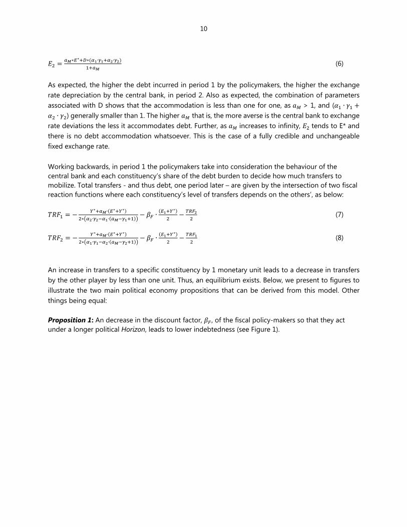
An increase in transfers to a specific constituency by 1 monetary unit leads to a decrease in transfers by the other player by less than one unit. Thus, an equilibrium exists. Below, we present to figures to illustrate the two main political economy propositions that can be derived from this model. Other things being equal: Proposition 1: An decrease in the discount factor, , of the fiscal policy-makers so that they act under a longer political Horizon, leads to lower indebtedness (see Figure 1).

11

Figure 1. Political Horizon and Indebtedness

Note: A lower discount of the future (i.e., higher political Horizon) leads to lower indebtedness (i.e., more fiscal discipline).

Proposition 2: An increase in political Cohesion, expressed by a more even distribution of the debt burden between political constituencies, leads to a decrease in public debt (see Figure 2).

Figure 2. Political Cohesion and Indebtedness

Note: A higher level of burden sharing (i.e., higher political Cohesion) leads lower indebtedness (i.e., more fiscal discipline).

0

2

4

6

8

10

12

14

16

18

20

0 5 10 15 20

TR

F (

1)

TRF (2)

Transfers of Player 1(Initial Discount)

Transfers of Player 2(Initial Discount)

Transfers of Player 1(Lower Discount)

Transfers of Player 2(Lower Discount)

0

2

4

6

8

10

12

14

16

18

20

0 5 10 15 20

TR

F (

1)

TRF (2)

Transfers of Player 1(Equal Payment)

Transfers of Player 2(Equal Payment)

Transfers of Player 1(Unequal Payment)

Transfers of Player 2(Unequal Payment)

12

IV. EMPIRICAL ANALYSIS

Data Description To test the propositions above, we use an unbalanced panel of 79 countries, including 31 advanced countries and 48 emerging and low income economies, between the years of 1975 and 2012, to estimate the following specification:

itititititittiit POLERPOLERFD )*(' (9)

where itFD is our proxy for fiscal discipline, given by the primary balance, measured in percent of

GDP;13 itER is a dummy variable taking the value 1 when a country is under a fixed exchange rate

regime and 0 if under a flexible exchange rate regime;14 it' , which is a vector of control variables

expected to affect the fiscal policy stance comprised of: the real GDP growth rate, trade openness (exports plus imports as share of GDP), terms of trade, log of total reserves, in USD, private credit, in

percent of % GDP, and CPI inflation rate.15 The parameters ti , are country and time effects and aim

at capturing unobserved heterogeneity across countries and time-unvarying factors. it is a white

noise iid disturbance term satisfying standard assumptions of zero mean and constant variance. Finally,

itPOL accounts for political factors, which will be constructed using Principal Component Analysis -

hereafter PCA, to obtain the common factor(s) of each block of variables comprising two components we termed Horizon and Cohesion. These are defined as follows:

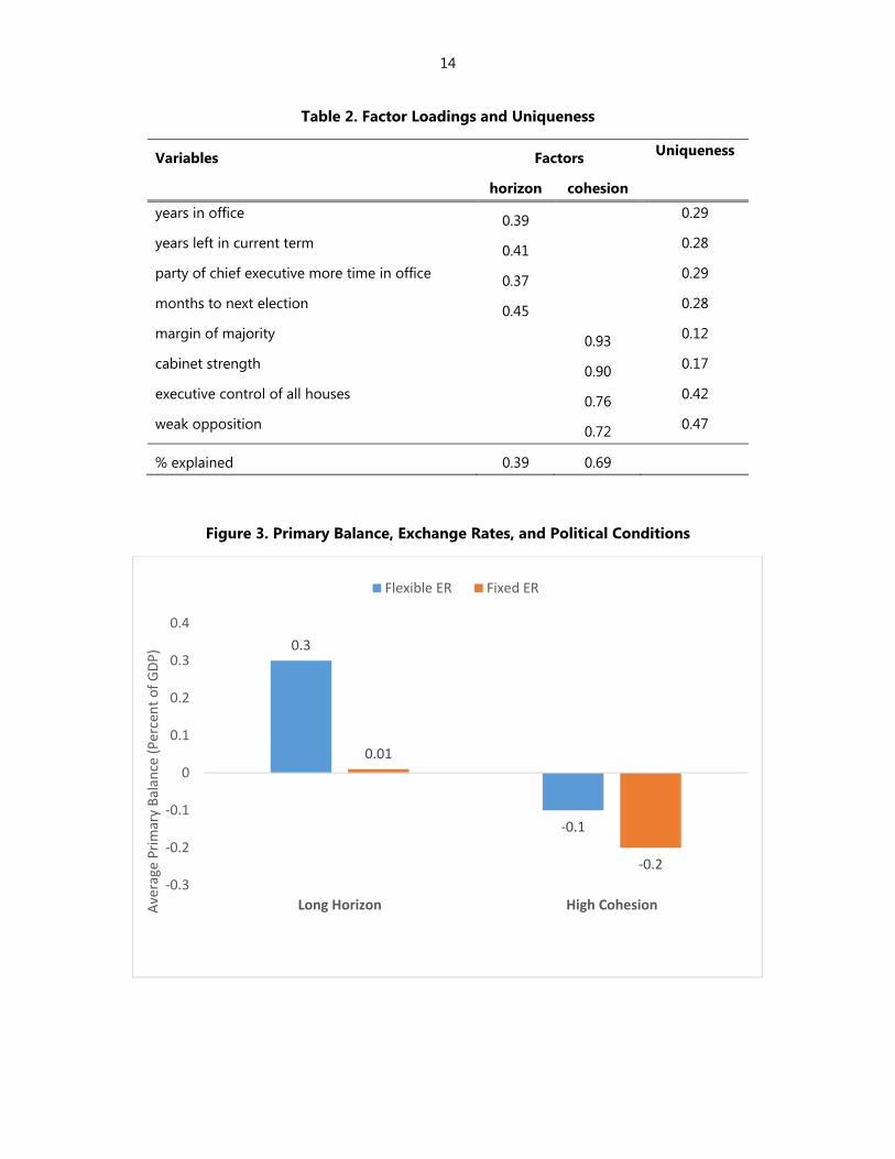
Political Horizon: a longer political horizon is associated with less years in office, more years left in current term, a party of chief executive with a long tradition in office, more months to next election.16 Only the first principal component is retained.17

Political Cohesion: a stronger political cohesion is associated with a high margin of the parliamentary majority supporting the cabinet, low cabinet fragmentation, executive control of all houses, and a weak opposition. Only the first principal component is retained.

13 Source: IMF’s International Financial Statistics. 14 We use the classification of exchange rate regimes provided by Reinhart and Rogoff’s (2004) and generate a dummy variable that takes value 1 (fixed exchange rate) if the country/year observation has any value between 1 and 8 in the Reinhart and Rogoff’s classification, and takes value zero otherwise – original Reinhart and Rogoff’s values of 9 to 15. We also test the robustness of our results by generating another dummy variable that uses Coarse’s classification from the IMF. 15 This is in line with Duttagupta and Tolosa (2006). 16 This latter indicator refers to actual months left to next election, ex-post facto, after the fact, while the variable “more years left in current term” is observed ex-ante. Both are informative. 17 A likelihood ratio (LR) test was used to examine the “sphericity” case, allowing for sampling variability in the correlations. This test comfortably rejects sphericity at the 1% level. The first factor explains almost 40% of the variance in the standardized data (see Table 2).

13

Horizon and Cohesion variables are each represented by one factor composed of four underlying variables.18 The resulting principal components indices are described in Table 1, while Table 2 lists the corresponding factor loadings.19 We can interpret the principal components by focusing on the factor loadings and the uniqueness of each variable.20 As regards political Horizon, uniqueness is relatively low for all variables, which implies that the factor retained spans the original variables adequately. As to political Cohesion, the factor appears to describe mostly the margin of majority and cabinet strength. In principle, both factors should enter with positive coefficients in the regressions.

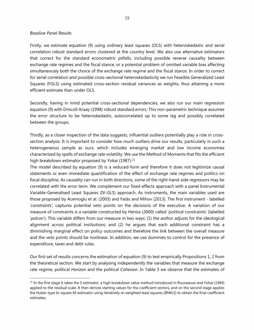
A first look at the data shows that in line with the findings of Tornell and Velasco (1995) and Sun (2003), fiscal discipline is lower under fixed exchange regimes than under flexible ones (see Figure 3). Also, stylized facts seem to confirm the propositions of the theoretical model presented above: in contexts of long political Horizon, the average primary surplus was only 0.01 percent of GDP under fixed exchange rate regimes and it reached up to 0.3 percent of GDP under flexible exchange rates. These differences were smaller in contexts of high political Cohesion. In this case, the average primary deficit was -0.2 percent of GDP under fixed exchange rates and slightly better, at -0.1 percent of GDP.

Table 1. Summary of Political Composite Variables and Descriptive Statistics Concept Average Standard deviation Variables

Horizon 0 1 years in office

years left in current term

party of chief executive more time in office

months to next election

Cohesion 0 1 margin of majority

cabinet strength

executive control of all houses

weak opposition

18 The sources for each component variable are the Database on Political Institutions (DPI, 2015). 19 PCA is based on the classical covariance matrix, which is sensitive to outliers. Here we conduct a robust estimation of the covariance matrix. A well suited method is the Minimum Covariance Determinant (MCD) that considers all subsets containing h % of the observations and estimates the variance of the mean on the data of the subset associated with the smallest covariance matrix determinant. Specifically, we implement the Rousseeuw and Van Driessen's (1999) algorithm. When we computed the same indices with the MCD version, we obtained similar results, suggesting that outliers are not driving our factor analysis. 20 Uniqueness of a variable is the share of its variance that is not accounted by all the factors.

14

Table 2. Factor Loadings and Uniqueness

Variables Factors Uniqueness

horizon cohesion

years in office 0.39 0.29

years left in current term 0.41 0.28

party of chief executive more time in office 0.37 0.29

months to next election 0.45 0.28

margin of majority 0.93 0.12

cabinet strength 0.90 0.17

executive control of all houses 0.76 0.42

weak opposition 0.72 0.47

% explained 0.39 0.69

Figure 3. Primary Balance, Exchange Rates, and Political Conditions

0.3

-0.1

0.01

-0.2

-0.3

-0.2

-0.1

0

0.1

0.2

0.3

0.4

Long Horizon High CohesionAve

rage

Pri

mar

y B

alan

ce (

Per

cen

t o

f G

DP

)

Flexible ER Fixed ER

15

Baseline Panel Results Firstly, we estimate equation (9) using ordinary least squares (OLS) with heteroskedastic and serial correlation robust standard errors clustered at the country level. We also use alternative estimators that correct for the standard econometric pitfalls, including possible reverse causality between exchange rate regimes and the fiscal stance, or a potential problem of omitted variable bias affecting simultaneously both the choice of the exchange rate regime and the fiscal stance. In order to correct for serial correlation and possible cross-sectional heteroskedasticity we run Feasible Generalized Least Squares (FGLS) using estimated cross-section residual variances as weights, thus attaining a more efficient estimate than under OLS. Secondly, having in mind potential cross-sectional dependencies, we also run our main regression equation (9) with Driscoll-Kraay (1998) robust standard errors. This non-parametric technique assumes the error structure to be heteroskedastic, autocorrelated up to some lag and possibly correlated between the groups. Thirdly, as a closer inspection of the data suggests, influential outliers potentially play a role in cross-section analysis. It is important to consider how much outliers drive our results, particularly in such a heterogeneous sample as ours, which includes emerging market and low income economies characterized by spells of exchange rate volatility. We use the Method of Moments that fits the efficient high breakdown estimator proposed by Yokai (1987).21 The model described by equation (9) is a reduced-form and therefore it does not legitimize causal statements or even immediate quantification of the effect of exchange rate regimes and politics on fiscal discipline. As causality can run in both directions, some of the right-hand-side regressors may be correlated with the error term. We complement our fixed-effects approach with a panel Instrumental Variable-Generalised Least Squares (IV-GLS) approach. As instruments, the main variables used are those proposed by Acemoglu et al. (2003) and Fatàs and Mihov (2013). The first instrument - labelled ‘constraints’, captures potential veto points on the decisions of the executive. A variation of our measure of constraints is a variable constructed by Henisz (2000) called ‘political constraints’ (labelled ‘polcon’). This variable differs from our measure in two ways: (1) the author adjusts for the ideological alignment across political institutions; and (2) he argues that each additional constraint has a diminishing marginal effect on policy outcomes and therefore the link between the overall measure and the veto points should be nonlinear. In addition, we use dummies to control for the presence of expenditure, taxes and debt rules. Our first set of results concerns the estimation of equation (9) to test empirically Propositions 1, 2 from the theoretical section. We start by analysing independently the variables that measure the exchange rate regime, political Horizon and the political Cohesion. In Table 3 we observe that the estimates of

21 In the first stage it takes the S estimator, a high breakdown value method introduced in Rousseeuw and Yohai (1984) applied to the residual scale. It then derives starting values for the coefficient vectors, and on the second stage applies the Huber-type bi-square M-estimator using iteratively re-weighted least squares (IRWLS) to obtain the final coefficient estimates.

16

the coefficient associated with the fixed exchange rate regime is always negative and almost always statistically significant at conventional levels. These results are in line with the latest findings in the empirical literature: being in or moving to a fixed exchange rate regime is associated with less fiscal discipline. Also, theoretical Propositions 1 and 2 are confirmed empirically as well. A longer political Horizon and more political Cohesion are both associated with a higher primary balance and more fiscal discipline. The rest of the controls are usually statistically significant and with the expected sign: higher GDP growth, higher inflation, higher reserves, better terms of trade and trade and financial openness are all associated with higher fiscal discipline.22

Table 3. Baseline, Fixed Effects Regressions Specification (1) (2) (3) (4) (5) (6) (7) Fixed ER -0.432** -0.412** -0.366* -0.388* -0.406* -0.472** -0.370 (0.180) (0.192) (0.219) (0.230) (0.215) (0.226) (0.234) Growth 0.087*** 0.098*** 0.116*** 0.100*** 0.116*** 0.135*** 0.145*** (0.019) (0.020) (0.021) (0.024) (0.020) (0.022) (0.023) Trade Openness 0.017*** 0.015*** 0.021*** 0.019*** 0.021*** 0.012* 0.012* (0.005) (0.005) (0.006) (0.006) (0.006) (0.006) (0.007) Terms Of Trade 0.017*** 0.018*** 0.020*** 0.028*** 0.016*** 0.016*** 0.018*** (0.003) (0.003) (0.004) (0.004) (0.004) (0.005) (0.005) Reserves 0.438*** 0.410*** 0.451*** 0.398*** 0.271*** 0.217** 0.226** (0.093) (0.093) (0.108) (0.101) (0.099) (0.102) (0.107) Inflation 0.034*** 0.024** 0.030*** 0.027*** (0.011) (0.011) (0.010) (0.010) Financial Openness

0.017*

(0.009) Credit 0.045*** (0.013) Horizon 0.346*** 0.310*** (0.096) (0.116) Cohesion 0.241* 0.241 (0.142) (0.164) Observations 2,404 2,216 1,888 1,779 1,808 1,560 1,456 R-squared 0.442 0.456 0.476 0.471 0.486 0.478 0.478

Note: Estimation with country and time effects (omitted for reasons of parsimony). Robust standard errors clustered at the country level in parenthesis. Constant term estimated by omitted. *, **, *** denote statistical significance at the 1, 5 and 10 percent levels, respectively.

In Table 4 we include two interaction terms between the dummy variable for fixed exchange rate regimes and the two variables that measure political Horizon and Cohesion. Again, we obtain a statistically significant and negative estimate of the coefficient on fixed exchange rate regimes and positive coefficients for both political indicators. Interestingly, the interaction terms between the key variables are negative suggesting that the positive effect of politics (longer Horizon or higher Cohesion) on the degree of fiscal discipline are particularly relevant for flexible exchange rate regimes. In other words, it is in flexible exchange rate settings that politics seems to matter most.

22 For reasons of parsimony, for the remainder of the paper we refrain from commenting on the controls.

17

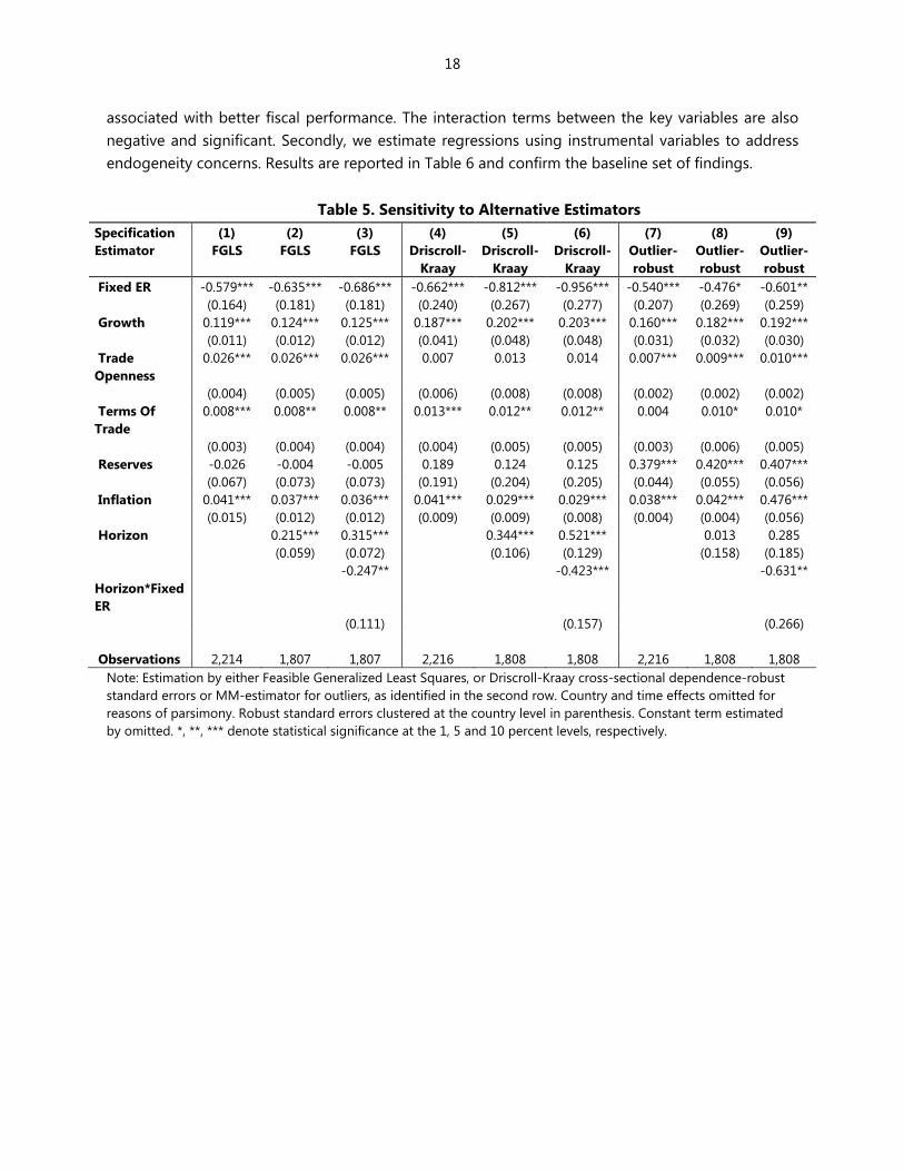
Note that these results shed light on the questions that motivate this paper. In line with our model´s prediction, both exchange rates and politics matter for fiscal discipline. In line with our model’s prediction, flexible (not fixed) exchange rates, and strong politics (long horizon and high cohesion) are both associated with better fiscal positions. The exchange rate regime seems to be quantitatively more important than the underlying political conditions. When considered together, strong politics attenuate the damaging effects of fixed rates on fiscal discipline, but are insufficient to reverse fiscal profligacy. Moreover, the positive effects of longer political horizon and more political cohesion on fiscal performance are amplified under flexible exchange rate regimes.

Table 4. Interaction Terms, Fixed Effects Regressions

Specification (1) (2) (3) (4) (5) (6) Fixed ER -0.637*** -0.826*** -0.720*** -0.547** -0.696*** -0.589** (0.208) (0.236) (0.263) (0.214) (0.262) (0.267) Growth 0.111*** 0.126*** 0.135*** 0.117*** 0.135*** 0.145*** (0.020) (0.022) (0.023) (0.020) (0.022) (0.023) Trade Openness 0.025*** 0.014** 0.016** 0.022*** 0.011* 0.012* (0.006) (0.006) (0.007) (0.006) (0.006) (0.007) Terms Of Trade 0.016*** 0.017*** 0.019*** 0.016*** 0.016*** 0.018*** (0.003) (0.005) (0.005) (0.004) (0.005) (0.005) Reserves 0.260*** 0.208** 0.214** 0.273*** 0.207** 0.224** (0.095) (0.098) (0.103) (0.099) (0.102) (0.107) Horizon 0.534*** 0.451*** 0.519*** 0.433*** (0.114) (0.144) (0.117) (0.148) Horizon*Fixed ER -0.435*** -0.308 -0.417** -0.278 (0.167) (0.225) (0.171) (0.233) Cohesion 0.370** 0.288 0.364** 0.296 (0.169) (0.181) (0.175) (0.181) Cohesion*Fixed ER -0.397* -0.178 -0.343 -0.146 (0.231) (0.287) (0.259) (0.294) Inflation 0.024** 0.029*** 0.027*** (0.010) (0.010) (0.010) Observations 1,904 1,655 1,534 1,808 1,560 1,456 R-squared 0.485 0.470 0.472 0.488 0.478 0.479

Note: Estimation with country and time effects (omitted for reasons of parsimony). Robust standard errors clustered at the country level in parenthesis. Constant term estimated by omitted. *, **, *** denote statistical significance at the 1, 5 and 10 percent levels, respectively.

V. ROBUSTNESS CHECKS

Sensitivity to alternative estimators, outliers and endogeneity To test the robustness of our baseline results, we perform a series of robustness checks. First, we re-estimate equation (9) using FGLS, Driscroll-Kraay cross-sectional dependence-robust standard errors and also the MM-estimator to check for outliers. Results in Table 5 show again that fixed exchange rates are associated with less fiscal discipline, while a longer Horizon (and higher Cohesion 23 is

23 Results for Cohesion are available from the authors upon request.

18

associated with better fiscal performance. The interaction terms between the key variables are also negative and significant. Secondly, we estimate regressions using instrumental variables to address endogeneity concerns. Results are reported in Table 6 and confirm the baseline set of findings.

Table 5. Sensitivity to Alternative Estimators

Specification (1) (2) (3) (4) (5) (6) (7) (8) (9) Estimator FGLS FGLS FGLS Driscroll-

Kraay Driscroll-

Kraay Driscroll-

Kraay Outlier-robust

Outlier-robust

Outlier-robust

Fixed ER -0.579*** -0.635*** -0.686*** -0.662*** -0.812*** -0.956*** -0.540*** -0.476* -0.601** (0.164) (0.181) (0.181) (0.240) (0.267) (0.277) (0.207) (0.269) (0.259) Growth 0.119*** 0.124*** 0.125*** 0.187*** 0.202*** 0.203*** 0.160*** 0.182*** 0.192*** (0.011) (0.012) (0.012) (0.041) (0.048) (0.048) (0.031) (0.032) (0.030) Trade Openness

0.026*** 0.026*** 0.026*** 0.007 0.013 0.014 0.007*** 0.009*** 0.010***

(0.004) (0.005) (0.005) (0.006) (0.008) (0.008) (0.002) (0.002) (0.002) Terms Of Trade

0.008*** 0.008** 0.008** 0.013*** 0.012** 0.012** 0.004 0.010* 0.010*

(0.003) (0.004) (0.004) (0.004) (0.005) (0.005) (0.003) (0.006) (0.005) Reserves -0.026 -0.004 -0.005 0.189 0.124 0.125 0.379*** 0.420*** 0.407*** (0.067) (0.073) (0.073) (0.191) (0.204) (0.205) (0.044) (0.055) (0.056) Inflation 0.041*** 0.037*** 0.036*** 0.041*** 0.029*** 0.029*** 0.038*** 0.042*** 0.476*** (0.015) (0.012) (0.012) (0.009) (0.009) (0.008) (0.004) (0.004) (0.056) Horizon 0.215*** 0.315*** 0.344*** 0.521*** 0.013 0.285 (0.059) (0.072) (0.106) (0.129) (0.158) (0.185) Horizon*Fixed ER

-0.247** -0.423*** -0.631**

(0.111) (0.157) (0.266) Observations 2,214 1,807 1,807 2,216 1,808 1,808 2,216 1,808 1,808

Note: Estimation by either Feasible Generalized Least Squares, or Driscroll-Kraay cross-sectional dependence-robust standard errors or MM-estimator for outliers, as identified in the second row. Country and time effects omitted for reasons of parsimony. Robust standard errors clustered at the country level in parenthesis. Constant term estimated by omitted. *, **, *** denote statistical significance at the 1, 5 and 10 percent levels, respectively.

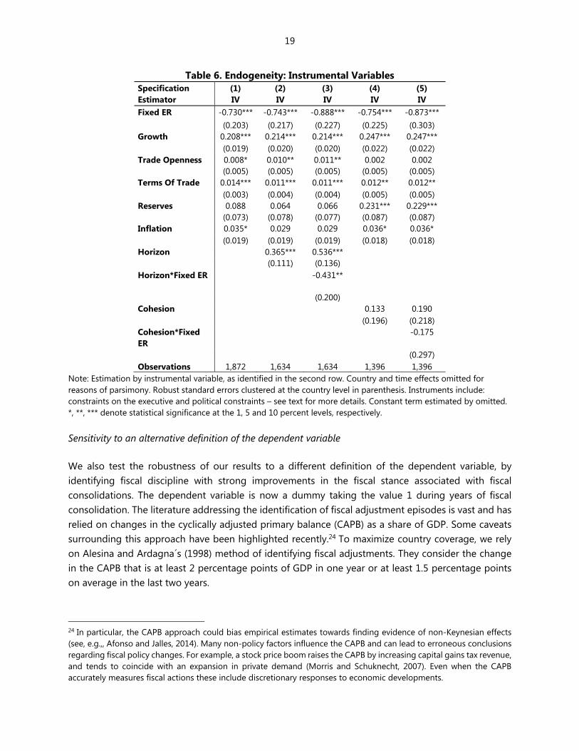
19

Table 6. Endogeneity: Instrumental Variables Specification (1) (2) (3) (4) (5) Estimator IV IV IV IV IV Fixed ER -0.730*** -0.743*** -0.888*** -0.754*** -0.873*** (0.203) (0.217) (0.227) (0.225) (0.303) Growth 0.208*** 0.214*** 0.214*** 0.247*** 0.247*** (0.019) (0.020) (0.020) (0.022) (0.022) Trade Openness 0.008* 0.010** 0.011** 0.002 0.002 (0.005) (0.005) (0.005) (0.005) (0.005) Terms Of Trade 0.014*** 0.011*** 0.011*** 0.012** 0.012** (0.003) (0.004) (0.004) (0.005) (0.005) Reserves 0.088 0.064 0.066 0.231*** 0.229*** (0.073) (0.078) (0.077) (0.087) (0.087) Inflation 0.035* 0.029 0.029 0.036* 0.036* (0.019) (0.019) (0.019) (0.018) (0.018) Horizon 0.365*** 0.536*** (0.111) (0.136) Horizon*Fixed ER -0.431**

(0.200) Cohesion 0.133 0.190 (0.196) (0.218) Cohesion*Fixed ER

-0.175

(0.297) Observations 1,872 1,634 1,634 1,396 1,396

Note: Estimation by instrumental variable, as identified in the second row. Country and time effects omitted for reasons of parsimony. Robust standard errors clustered at the country level in parenthesis. Instruments include: constraints on the executive and political constraints – see text for more details. Constant term estimated by omitted. *, **, *** denote statistical significance at the 1, 5 and 10 percent levels, respectively. Sensitivity to an alternative definition of the dependent variable

We also test the robustness of our results to a different definition of the dependent variable, by identifying fiscal discipline with strong improvements in the fiscal stance associated with fiscal consolidations. The dependent variable is now a dummy taking the value 1 during years of fiscal consolidation. The literature addressing the identification of fiscal adjustment episodes is vast and has relied on changes in the cyclically adjusted primary balance (CAPB) as a share of GDP. Some caveats surrounding this approach have been highlighted recently.24 To maximize country coverage, we rely on Alesina and Ardagna´s (1998) method of identifying fiscal adjustments. They consider the change in the CAPB that is at least 2 percentage points of GDP in one year or at least 1.5 percentage points on average in the last two years.

24 In particular, the CAPB approach could bias empirical estimates towards finding evidence of non-Keynesian effects (see, e.g.,, Afonso and Jalles, 2014). Many non-policy factors influence the CAPB and can lead to erroneous conclusions regarding fiscal policy changes. For example, a stock price boom raises the CAPB by increasing capital gains tax revenue, and tends to coincide with an expansion in private demand (Morris and Schuknecht, 2007). Even when the CAPB accurately measures fiscal actions these include discretionary responses to economic developments.

20

Since we now have a dependent variable that is expressed in binary terms, we employ a logistic regression to estimate equation (1). More precisely, we estimate the following model:25 Prob(FD 1|ER,X ) ( ' ),i ER POL X (10)

where , , , are vectors of the parameters to be estimated and (.) is the logistic function.26

Given that we rely on panel data, the structural model can be written as:

*it

*it it

FD ' ,

FD 1 if FD 0, and 0 otherwise.

i it itER POL

X (11)

with i = 1, …, 78; t = 1980, …, 2013; i captures the unobserved individual effects; and it is the error

term. We take the analysis one step further and also assume that a fiscal adjustment is successful (SU) if the improvement in the cyclically adjusted primary budget balances for two consecutive years is at least η-times the standard deviation of the cyclically adjusted primary budget balance in the full panel (see Afonso and Jalles, 2012):

1

0

1,

0,

t ii

if b

otherwise

(12)

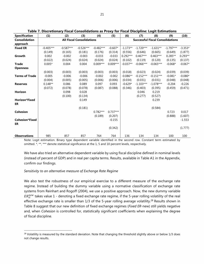
In our analysis we use a threshold value of η=1. Our results suggest that fixed exchange rate regimes decrease the likelihood of a given government engaging in a fiscal consolidation.27 More importantly, the likelihood is even smaller if we restrict our sample to successful fiscal episodes, as shown by the higher magnitude - in absolute value, of the estimated coefficients in columns 6 to 10. The Horizon of the policy-makers is never relevant, in line with results in Alesina, Perotti and Tavares (1998), which find that engaging in fiscal adjustments does not increase the likelihood of cabinet turnover. In this setting, political Cohesion becomes statistically irrelevant, as the interaction term between Cohesion and exchange rate regime loses statistical significance.

25 For details on this binary choice model see, for example, Greene (2012, Ch. 17). 26 As probit models do not render themselves well to the fixed-effects treatment due to the incidental parameter problem (Wooldridge, 2002, Ch. 15, p. 484), we estimate a logit model with fixed-effects. 27 As a robustness check to Alesina and Ardagna’s (1998) method we employed alternatively Giavazzi and Pagano’s (1996). They propose using the cumulative changes in the CAPB that are at least 5, 4, 3 percentage points of GDP in respectively 4, 3 or 2 years, or 3 percentage points in one year. Results, available upon request, did not qualitatively change.

21

Table 7. Discretionary Fiscal Consolidations as Proxy for Fiscal Discipline: Logit Estimations

Specification (1) (2) (3) (4) (5) (6) (7) (8) (9) (10) Consolidation approach

All Fiscal Consolidations Successful Fiscal Consolidations

Fixed ER -0.405*** -0.587*** -0.526*** -0.482*** -0.607* -1.173** -1.720*** -1.631** -1.797*** -3.353* (0.149) (0.165) (0.181) (0.176) (0.314) (0.556) (0.646) (0.665) (0.649) (1.877)Growth 0.002 -0.002 -0.003 -0.033 -0.033 0.292*** 0.467*** 0.463*** 0.285** 0.293** (0.022) (0.024) (0.024) (0.024) (0.024) (0.102) (0.119) (0.120) (0.135) (0.137)Trade Openness

0.005* 0.004 0.004 0.009*** 0.009*** -0.037** -0.066*** -0.065*** -0.068* -0.067*

(0.003) (0.003) (0.003) (0.003) (0.003) (0.018) (0.023) (0.024) (0.039) (0.039)Terms of Trade -0.005 -0.006 -0.006 -0.002 -0.002 -0.086** -0.152*** -0.151*** -0.081* -0.080* (0.004) (0.005) (0.005) (0.006) (0.006) (0.034) (0.031) (0.031) (0.048) (0.048)Reserves 0.148** 0.086 0.089 0.097 0.093 -0.629* -1.103*** -1.078*** -0.204 -0.226 (0.072) (0.078) (0.078) (0.087) (0.088) (0.346) (0.403) (0.395) (0.459) (0.471)Horizon 0.098 0.028 0.046 0.219 (0.100) (0.134) (0.277) (0.527) Horizon*Fixed ER

0.149 0.239

(0.181) (0.584) Cohesion 0.782*** 0.737*** 0.723 0.017 (0.189) (0.207) (0.888) (1.607)Cohesion*Fixed ER

-0.155 -1.553

(0.342) (1.777) Observations 985 857 857 764 764 136 134 134 100 100

Note: Logit estimation. Binary type dependent variable identified in the second row. Constant term estimated by omitted. *, **, *** denote statistical significance at the 1, 5 and 10 percent levels, respectively. We have also tried an alternative dependent variable by using fiscal discipline defined in nominal levels (instead of percent of GDP) and in real per capita terms. Results, available in Table A1 in the Appendix, confirm our findings.

Sensitivity to an alternative measure of Exchange Rate Regime

We also test the robustness of our empirical exercise to a different measure of the exchange rate regime. Instead of building the dummy variable using a normative classification of exchange rate systems from Reinhart and Rogoff (2004), we use a positive approach. Now, the new dummy variable

takes value 1 - denoting a fixed exchange rate regime, if the 5-year rolling volatility of the real effective exchange rate is smaller than 1/3 of the 5-year rolling average volatility.28 Results shown in Table 8 suggest that our new definition of fixed exchange regimes (Fixed ER-new) still yields negative and, when Cohesion is controlled for, statistically significant coefficients when explaining the degree of fiscal discipline.

28 Volatility is measured by the standard deviation. Note that changing the threshold slightly above or below 1/3 does not change results.

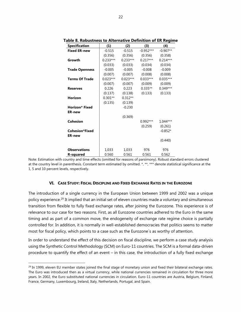
22

Table 8. Robustness to Alternative Definition of ER Regime Specification (1) (2) (3) (4) Fixed ER-new -0.515 -0.515 -0.952*** -0.907** (0.356) (0.356) (0.356) (0.358) Growth 0.233*** 0.233*** 0.217*** 0.214*** (0.033) (0.033) (0.034) (0.034) Trade Openness -0.005 -0.005 -0.008 -0.009 (0.007) (0.007) (0.008) (0.008) Terms Of Trade 0.023*** 0.023*** 0.033*** 0.035*** (0.007) (0.007) (0.009) (0.009) Reserves 0.226 0.223 0.335** 0.349*** (0.137) (0.138) (0.133) (0.133) Horizon 0.301** 0.312** (0.135) (0.139) Horizon* Fixed ER-new

-0.230

(0.369) Cohesion 0.992*** 1.044*** (0.259) (0.261) Cohesion*Fixed ER-new

-0.852*

(0.440) Observations 1,033 1,033 976 976 R-squared 0.560 0.561 0.561 0.562

Note: Estimation with country and time effects (omitted for reasons of parsimony). Robust standard errors clustered at the country level in parenthesis. Constant term estimated by omitted. *, **, *** denote statistical significance at the 1, 5 and 10 percent levels, respectively.

VI. CASE STUDY: FISCAL DISCIPLINE AND FIXED EXCHANGE RATES IN THE EUROZONE

The introduction of a single currency in the European Union between 1999 and 2002 was a unique policy experience.29 It implied that an initial set of eleven countries made a voluntary and simultaneous transition from flexible to fully fixed exchange rates, after joining the Eurozone. This experience is of relevance to our case for two reasons. First, as all Eurozone countries adhered to the Euro in the same timing and as part of a common move, the endogeneity of exchange rate regime choice is partially controlled for. In addition, it is normally in well-established democracies that politics seems to matter most for fiscal policy, which points to a case such as the Eurozone´s as worthy of attention.

In order to understand the effect of this decision on fiscal discipline, we perform a case study analysis using the Synthetic Control Methodology (SCM) on Euro-11 countries. The SCM is a formal data-driven procedure to quantify the effect of an event – in this case, the introduction of a fully fixed exchange

29 In 1999, eleven EU member states joined the final stage of monetary union and fixed their bilateral exchange rates. The Euro was introduced then as a virtual currency, while national currencies remained in circulation for three more years. In 2002, the Euro substituted national currencies in circulation. Euro-11 countries are Austria, Belgium, Finland, France, Germany, Luxembourg, Ireland, Italy, Netherlands, Portugal, and Spain.

23

rate in the Eurozone, on an outcome variable – here, the primary budget balance. The method relies on the creation of an artificial counterfactual that mimics the primary budget balance before the introduction of the single currency, using data on a set of variables from the years prior to the event, and then comparing the actual outcomes and with the counterfactual for the years after the event.30

The counterfactual – synthetic unit – is constructed as a weighted average of the primary budget balance in countries that have similar characteristics to the country under consideration but subsequently unaffected by the event.31 Country weights are chosen to minimize the distance between the country under consideration and its counterfactual in terms of the primary balance variable and its predictors (Abadie and others, 2010). The effect of an event is obtained as the difference between the outcome variable for the country in question and the weighted average of the outcome variable for the synthetic control group.

Figure 4 plots a number of important results from the SCM exercise which confirm our theoretical predictions and the main empirical results. The first chart in Figure 5 shows that, in the aftermath of moving to fixed exchange rates, Euro-11 maintained a lower primary balance than its synthetic counterfactual. In addition, Figure 5 shows results for four countries with extreme scores in terms of political Horizon and Cohesion vis-à-vis the principal component’s average value (PCA). Countries with high relative scores in at least one of the two political dimensions, such as Austria (higher-than-average horizon) or Portugal (higher-than-average cohesion), even if they experienced less fiscal discipline after joining the Eurozone they display a narrower distance with their synthetic counterfactuals. On the contrary, countries with lower-than-average scores in both political dimensions – such as Belgium-, saw their distance to the counterfactual increase. Finally, countries with higher-than-average scores both in terms of political horizon and cohesion (Spain) managed to improve fiscal discipline way above their synthetic counterfactual, proving that strong politics partially compensates from the negative fiscal effect of moving to fixed exchange rates.32

30 See Appendix 2 for more details. 31 These control countries included in the synthetic unit are, in our case, OECD member countries other than those under analysis (Euro-11). We also exclude transition economies. See Appendix 2. 32 In the case of Spain, we replicated the analysis using structural balance concept, to control for the potential effect on the primary balance stemming from the real estate bubble that increased fiscal revenues considerably during the late nineties. Results remain unchanged: while Spain could have adjusted further, it still performed better after the introduction of the euro.

24

Figure 4. Synthetic Control Analysis, Euro-11

25

VII. CONCLUSION

In this paper we present both theoretical and empirical evidence showing that, contrary to the traditional argument, flexible (not fixed) exchange rate regimes are associated with more fiscal discipline. The fiscal implications of exchange rate regime choice do not occur in a vacuum, but within a specific political context. By bringing politics into the picture, this paper contributes to the literature by carefully uncovering how the exchange rate regime interacts with the political context to affect fiscal policy outcomes. Our results draw on the longest and widest cross-section of country experiences available. We find that strong political environments characterized by long Horizon and high Cohesion among policy-makers (i.e., where elections are not imminent and where there is little political fragmentation) are associated with better fiscal performance.33 Our results offer important policy lessons from the point of view of fiscal policy making. First, if policymakers operate in weak political contexts, flexible exchange rates are the preferred option as they are best suited to secure enhanced fiscal discipline. Second, the virtuous effect of flexible exchange rates on fiscal discipline can be maximized by strong political environments, characterized by long political horizon and high political cohesion. Third, in mixed political contexts policy-makers face a difficult choice as moving to a fixed exchange rate regime may negatively impact fiscal performance in a way that political institutions are unable to attenuate.

33 In a recent paper making use of a laboratory experiment, Battaglini, Nunnari and Palfrey (2016) find evidence that more inclusive requirements for fiscal decision and more vulnerability to shocks (which we can equate to longer horizons) are associated with lower debt accumulation.

26

APPENDIX 1. ROBUSTNESS

Table A1. Robustness to Alternative Measures of Fiscal Discipline

Specification (1) (2) (3) (4) (5) (6) (7) (8) (9) (10) Dep. Variable Nominal Primary Balance Real Primary Balance per capita Fixed ER -0.926*** -0.385 -0.424 -0.618* -0.233 -0.881*** -0.369 -0.411 -0.603* -0.206 (0.316) (0.301) (0.338) (0.393) (0.369) (0.313) (0.298) (0.335) (0.389) (0.366) Growth -0.006 0.030 0.030 0.042 0.041 -0.005 0.030 0.030 0.043 0.042 (0.034) (0.029) (0.029) (0.036) (0.036) (0.034) (0.029) (0.029) (0.035) (0.036) Trade Openness -0.034*** -0.022*** -0.022*** -0.039*** -0.038*** -0.034*** -0.022*** -0.022*** -0.039*** -0.038*** (0.007) (0.006) (0.006) (0.010) (0.010) (0.007) (0.006) (0.006) (0.010) (0.010) Terms Of Trade -0.006 -0.002 -0.002 -0.008 -0.008 -0.006 -0.002 -0.002 -0.008 -0.008 (0.006) (0.004) (0.004) (0.006) (0.006) (0.006) (0.004) (0.004) (0.006) (0.006) Reserves 0.625*** 0.460*** 0.462*** 0.832*** 0.840*** 0.592*** 0.427*** 0.429*** 0.813*** 0.821*** (0.138) (0.114) (0.114) (0.152) (0.152) (0.137) (0.113) (0.113) (0.150) (0.151) Horizon -0.154 -0.121 -0.149 -0.114 (0.104) (0.140) (0.104) (0.139) Horizon*Fixed ER -0.088 -0.093 (0.202) (0.201) Cohesion 0.909*** 0.746** 0.943*** 0.775** (0.291) (0.307) (0.288) (0.304) Cohesion*Fixed ER

0.566 0.584

(0.387) (0.383) Observations 1,121 896 896 800 800 1,121 896 896 800 800 R-squared 0.740 0.762 0.762 0.737 0.738 0.741 0.756 0.756 0.736 0.737

Note: Dependent variable identified in second row. Estimation with country and time effects (omitted for reasons of parsimony). Robust standard errors clustered at the country level in parenthesis. Constant term estimated by omitted. *, **, *** denote statistical significance at the 1, 5 and 10 percent levels, respectively.

27

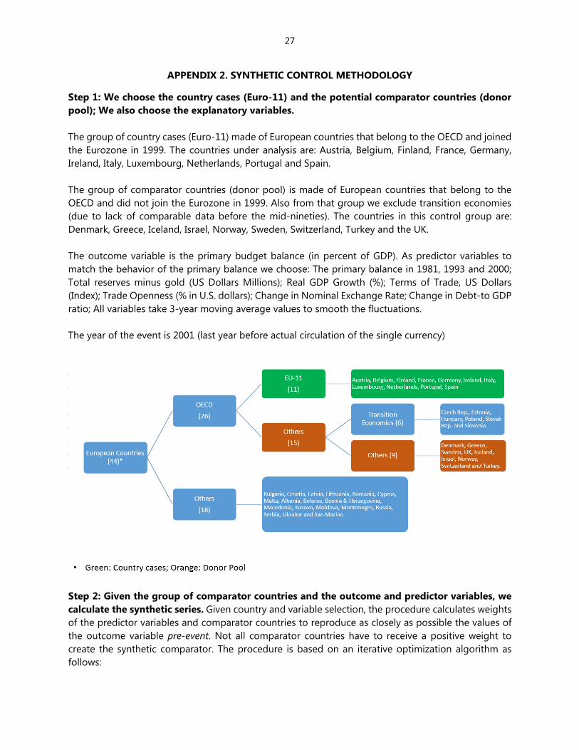
APPENDIX 2. SYNTHETIC CONTROL METHODOLOGY

Step 1: We choose the country cases (Euro-11) and the potential comparator countries (donor pool); We also choose the explanatory variables. The group of country cases (Euro-11) made of European countries that belong to the OECD and joined the Eurozone in 1999. The countries under analysis are: Austria, Belgium, Finland, France, Germany, Ireland, Italy, Luxembourg, Netherlands, Portugal and Spain. The group of comparator countries (donor pool) is made of European countries that belong to the OECD and did not join the Eurozone in 1999. Also from that group we exclude transition economies (due to lack of comparable data before the mid-nineties). The countries in this control group are: Denmark, Greece, Iceland, Israel, Norway, Sweden, Switzerland, Turkey and the UK. The outcome variable is the primary budget balance (in percent of GDP). As predictor variables to match the behavior of the primary balance we choose: The primary balance in 1981, 1993 and 2000; Total reserves minus gold (US Dollars Millions); Real GDP Growth (%); Terms of Trade, US Dollars (Index); Trade Openness (% in U.S. dollars); Change in Nominal Exchange Rate; Change in Debt-to GDP ratio; All variables take 3-year moving average values to smooth the fluctuations. The year of the event is 2001 (last year before actual circulation of the single currency)

Step 2: Given the group of comparator countries and the outcome and predictor variables, we calculate the synthetic series. Given country and variable selection, the procedure calculates weights of the predictor variables and comparator countries to reproduce as closely as possible the values of the outcome variable pre-event. Not all comparator countries have to receive a positive weight to create the synthetic comparator. The procedure is based on an iterative optimization algorithm as follows:

28

Start from some initial vector of weights of the predictor variables V, choose the vector ∗ of country weights to minimize a distance ‖ ‖ where and are matrices of predictor variables for the unit of interest and its comparator units, respectively, subject to weight constraints (weights have to be between 0 and 1). In particular, ∗ minimizes

‖ ‖ ′ 1

Once the country weights are chosen, the variable weight ∗ is chosen among all positive

definite and diagonal matrices such that the mean square prediction error (MSPE) of the outcome variable is minimized over pre-event periods. In particular:

∗ min∈

∗ ′ ∗ 2

where and are matrices of the outcome variable for the unit of interest and its comparator units, respectively. The resulting ∗ is used as input to (1) for the next round of optimization.

This iterative process continues until both ∗ and ∗ converge. In summary, the synthetic series are constructed by solving a nested optimization problem that minimizes (2) for given

∗ given by (1) (Abadie and others, 2011).

Using the weights thus obtained, we then use the synthetic comparator to create a counterfactual path of the outcome variable post-event.

Step 3: Compare actual post-event outcome variable series with the synthetic comparator. The difference between the two series is the estimated impact of the event (assuming that all other factors potentially affecting the variable of interest have been controlled for successfully).

29

REFERENCES

Abadie, A., A. Diamond, and J. Hainmueller, (2010), “Synthetic Control Methods for Comparative Case Studies: Estimating the Effect of California's Tobacco Control Program,” Journal of the American Statistical Association, 105 (490): pp. 493-505

Acemoglu, Daron, Simon Johnson, James Robinson, and Y. Thaicharoen (2003), “Institutional causes, macroeconomic symptoms: volatility, crises and growth,” Journal of Monetary Economics 50, pp. 49-123.

Afonso, A. and Jalles, J. T. (2012), “Measuring the Success of Fiscal Consolidations”, Applied Financial Economics, Vol. 22(13)

Afonso, A. and Jalles, J. T. (2014), “Assessing Fiscal Episodes”, Economic Modelling, Vol. 37, pp. 255-270

Alesina, A., Ardagna, S. (1998). “Tales of Fiscal Contractions,” Economic Policy, 27, 487-545.

Alesina, A., Perotti, R., and J. Tavares (1998), “The Political Economy of Fiscal Adjustments”, Brookings Papers in Political Economy, Vol. 1, pp. 197-266.

Battaglini, M., Nunnari, S., and T. R. Palfrey (2016), “The Political Economy of Public Debt: A Laboratory Study”, CEPR Discussion Paper n. 11357

Bordo, M. (2003), “Exchange Rate Regime Choice in Historical Perspective”, NBER Working Paper 9654

Bowsher, C. (2002): “On Testing Over-identifying Restrictions in Dynamic Panel Data Models,” Economic Letters, 77(2), 211—220.

Duttagupta, R., and G. Tolosa, 2006, “Fiscal Discipline and Exchange Rate Regimes: Evidence from the Caribbean,” IMF Working Paper, 06/119, (Washington D.C.: International Monetary Fund).

Fatás, A. and A. K. Rose (2001) Do monetary handcuffs restrain Leviathan? Fiscal policy in extreme exchange rate regimes, IMF Staff Papers, 47, 40-61.

Fatás, A., and I. Mihov 2013. “Policy Volatility, Institutions and Economic Growth.” Review of Economics and Statistics 95 (2): 362–76.

Frankel, J., M. Goldstein, and P. Masson (1991), “Characteristics of a Successful Exchange Rate System”; IMF occasional paper Nº82.

Gavin, M., and R. Perotti. 1997. "Fiscal Policy in Latin America." In NBER Macroeconomics Annual 1997, edited by Ben S. Bernanke and Julio Rotemberg. MIT Press.

Giavazzi, F. and M. Pagano (1988), “The Advantage of Tying One’s hands: EMS Discipline and Central Bank Credibility”; European Economic Review, June.

Giavazzi, F., Pagano, M. (1996). “Non-Keynesian Effects of Fiscal Policy Changes: International Evidence and the Swedish Experience,” Swedish Economic Policy Review, 3 (1), 67-103.

Lambertini, L., and Tavares, J. (2005), “Exchange Rates and Fiscal Adjustments: Evidence from the OECD and Implications for the EMU”, BEJM Contributions in Macroeconomics.

Lane, P., and Perotti, R. (2003), “The Importance of Composition of Fiscal Policy: Evidence from Different Exchange Rate Regimes”, Journal of Public Economics, Vol. 87, pp. 2253–2279.

30

Morris, R. and L. Schuknecht, 2007, “Structural Balances and Asset Windfalls: The Role of Asset Prices Revisited,” ECB Working Paper No. 737.

Muller, Wolfgang C. and Strom K. (eds.), 1999, Policy, Office or Votes? How Political Parties in Western Europe Make Hard Decisions. Cambridge: Cambridge University Press.

Reinhart, C. M. and K. S. Rogoff, 2004, “The Modern History of Exchange Rate Arrangements: A Reinterpretation,” The Quarterly Journal of Economics, vol. 119(1), pp. 1-48.

Roodman, D. (2009): “A Note on the Theme of Too Many Instruments,” Oxford Bulletin of Economics and Statistics, 71(1), 135—58.

Rousseeuw, P. J. and K. Van Driessen (1999). A fast algorithm for the minimum covariance determinant estimator. Technometrics 41, 212—223.

Rousseeuw, P.J. and Yohai, V. (1984), “Robust Regression by Means of S estimators”, in Robust and Nonlinear Time Series Analysis, edited by J. Franke, W. Härdle, and R.D. Martin, Lecture Notes in Statistics 26, Springer Verlag, New York, 256-274.

Sun, Y. (2003), “Do Fixed Exchange Rates Induce More Fiscal Discipline?”, IMF Working Paper N 03/78.

Tanzi V. and L. Schuknecht [1997]: Reconsidering the fiscal role of government: The international perspective, American Economic Review, 87, 164-172.

Tornell, A. and A. Velasco (1995), “Fiscal discipline and the choice of exchange rate regime”, European Economic Review, 39, 759-770.

Tornell, A. and A. Velasco (1998), “Fiscal Discipline and the Choice of a Nominal Anchor in Stabilization”, Journal of International Economics, Vol. 46, pp. 30.

Wooldridge, J.M. (2002), Econometric Analysis of Cross Section and Panel Data. MIT Press: Cambridge, MA.

Yohai, V. J. (1987), “High Breakdown-Point and High Efficiency Robust Estimates for Regression”, The Annals of Statistics, 15, 642-656.