Fiscal Foresight and Information Flows

Eric M. Leeper, Todd B. Walker, and Shu-Chun Susan Yang

WP/12/153

© 2012 International Monetary Fund WP/12/153

IMF Working Paper

Research Department

Fiscal Foresight and Information Flows*

Prepared by Eric M. Leeper, Todd B. Walker, and Shu-Chun Susan Yang

Authorized for distribution by Andrew Berg

June 2012

Abstract

News—or foresight—about future economic fundamentals can create rational expectations equilibria with non-fundamental representations that pose substantial challenges to econometric efforts to recover the structural shocks to which economic agents react. Using tax policies as a leading example of foresight, simple theory makes transparent the economic behavior and information structures that generate non-fundamental equilibria. Econometric analyses that fail to model foresight will obtain biased estimates of output multipliers for taxes; biases are quantitatively important when two canonical theoretical models are taken as data generating processes. Both the nature of equilibria and the inferences about the effects of anticipated tax changes hinge critically on hypothesized information flows. Different methods for extracting or hypothesizing the information flows are discussed and shown to bealternative techniques for resolving a non-uniqueness problem endemic to moving average representations.

JEL Classification Numbers:C5, E62, H30

Keywords: news, anticipated taxes, non-fundamental representation, identified VARs

Author’s E-Mail Address:eleeper@indiana.edu; walkertb@indiana.edu; syang@imf.org

* Department of Economics, Indiana University, Monash University and NBER, eleeper@indiana.edu; Department of Economics, Indiana University, walkertb@indiana.edu; International Monetary Fund, SYang@imf.org. Walker acknowledges support from NSF grant SES-0962221. Yang thanks Academia Sinica for support in the early stages of this research. We also acknowledge comments by Troy Davig, Mike Dotsey, Jesús Fernández-Villaverde, Dale Henderson, Beth Klee, Karel Mertens, Jim Nason, Ricardo Nunes, Valerie Ramey, Morten Ravn, Chris Sims, and participants at many conferences and presentations. Joonyoung Hur provided excellent research assistance. We are particularly grateful to Harald Uhlig and four anonymous referees for helpful comments.

This Working Paper should not be reported as representing the views of the IMF. The views expressed in this Working Paper are those of the author(s) and do not necessarily represent those of the IMF or IMF policy. Working Papers describe research in progress by the author(s) and are published to elicit comments and to further debate.

Contents Page I. Introduction ..........................................................................................................................3 II. Analytical Example ..............................................................................................................5

A. The Econometrics of Foresight ......................................................................................7 B. Generalizations ............................................................................................................12

III. Quantitative Importance of Foresight ................................................................................14 A. Modeling Information Flows .......................................................................................15 B. Model Descriptions ......................................................................................................17 C. Information Flows and Estimation Bias ......................................................................18

IV. Solving the Problem ...........................................................................................................20 A. An Organizing Principle ..............................................................................................21 B. Lines of Attack .............................................................................................................22

1. The Narrative Approach ........................................................................................22 2. Conditioning on Asset Prices .................................................................................24 3. Direct Estimation of DSGE Model ........................................................................27

V. Concluding Remarks ..........................................................................................................27

References ................................................................................................................................58 Tables 1. Information Flow Processes ..............................................................................................18 2. Output Multipliers for a Labor Tax Change .....................................................................20

Figures 1. Responses of Capital to Tax Increase ................................................................................10

Appendices I. Simulations Details ............................................................................................................29 II. Testing Economic Theory ..................................................................................................36 III. Municipal Bonds and Fiscal Foresight: Additional Results ..............................................38 IV. Assessing the Ex-Ante Approach ......................................................................................49

2

3

I. INTRODUCTION

A venerable tradition, often traced to Pigou (1927), ascribes a significant role in aggregate

fluctuations to economic decision makers’ responses to expectations about not-yet-realized

economic fundamentals. That tradition finds voice in a recent surge of interest in the

economic consequences of news—or foresight. Recent work explores how news affects the

predictions of standard theories, seeks evidence of the impacts of news in time series data,

and estimates dynamic stochastic general equilibrium models to quantify the relative

importance of anticipated and unanticipated “shocks” to fundamentals.

Existing work typically posits a particular stochastic process for news, grounded in neither

theory nor empirics. That process determines the economy’s information flows and, in a

rational expectations equilibrium, agents’ expectations. Given the prominent role of

expectations in the news literature, it is remarkable that existing work does not systematically

examine how the specification of information flows affects the nature of equilibrium and the

connection of theory to data. This paper addresses that gap.

For several reasons we focus on how to identify and quantify the impacts of foreseen

“shocks” to taxes. First, few economic phenomena provide economic agents with such clear

signals about how important margins will change in the future: foresight is intrinsic to tax

policy. Second, an institutional structure governs information flows about taxes: the process

of changing taxes entails two kinds of lags—the inside lag, between when new tax law is

initially proposed and when it is passed, and the outside lag, between when the legislation is

signed into law and when it is implemented. That institutional structure informs the nature of

tax information flows. Third, differential U.S. tax treatment of municipal and treasury bonds

leads to a direct measure of tax news that offers a potential solution to modeling tax

foresight. Such measures are scarce for news about nonpolicy fundamentals like total factor

productivity. Despite the paper’s focus on taxes, one of its key messages—that hypothesized

information flows are critical to determining the impacts of news—extends immediately to

other contexts.1

Fiscal foresight poses a challenge to econometric analyses of fiscal policy because it

generates an equilibrium with a non-fundamental moving average representation.

Information sets of economic agents and the econometrician can be misaligned, with agents

basing their choices on more information than the econometrician possesses. Structural

shocks to tax policy, then, cannot be recovered from current and past fiscal data, a central

assumption of conventional econometric methods. Instead, conventional methods can lead

1In addition to taxes, studies have examined news about a wide range of fundamentals, including total factor

and investment-specific productivity [Beaudry and Portier (2006), Christiano, Ilut, Motto, and Rostagno (2008),

Jaimovich and Rebelo (2009), Schmitt-Grohe and Uribe (2008), Fujiwara, Hirose, and Shintani (2011)];

government military spending run ups [Fisher and Peters (2010), Ramey (2011)]; phased-in governmentinfrastructure spending [Leeper, Walker, and Yang (2010)]; announcements of interest-rate paths by

inflation-targeting central banks [Blattner, Catenaro, Ehrmann, Strauch, and Turunen (2008), Laseen and

Svensson (2011)]. All of these applications lend themselves to the analysis that we conduct.

4

the econometrician to label as “tax shocks” objects that are linear combinations of all the

exogenous disturbances at various leads and lags.2

This paper builds on and extends Hansen and Sargent’s (1991b) general characterization of

the implications of environments in which the history of innovations in a vector

autoregression does not equal the history of information that agents observe. We go beyond

treating invertibility as a 0–1 proposition by assessing the quantitative importance of failing

to model foresight in two workhorse macroeconomic models. We offer a compelling

economic example—tax foresight—that makes clear that non-fundamentalness and its

consequences affect answers to substantive macroeconomic questions. Most importantly, we

ground non-fundamentalness in economic theory, which points towards empirical lines of

attack. Both Hansen and Sargent (1991b) and Fernandez-Villaverde, Rubio-Ramırez,

Sargent, and Watson (2007) have been read primarily as cautionary notes, in large part

because they point to a serious problem, but not to a way forward.

No consensus exists on how to handle tax foresight, a fact that is underscored by the diverse

empirical findings in the literature. Research concludes that an anticipated cut in taxes may

have little or no effect [Poterba (1988), Blanchard and Perotti (2002), Romer and Romer

(2010)], may be mildly expansionary in the short run [Mountford and Uhlig (2009)], or may

be strongly contractionary in the short run [House and Shapiro (2006), Mertens and Ravn

(2011)]. By using different measures of tax news and different methodologies, these studies

implicitly posit different tax information flows, which, as we show, can produce strikingly

different inferences about the effects of anticipated tax changes.

The paper has three parts:

1. A simple analytical example makes precise how foresight and optimizing behavior

create equilibria with non-fundamental moving average representations. The example

makes the source of non-fundamentalness transparent: it arises as a natural by-product

of the fact that agents’ optimal intertemporal decisions discount future tax obligations.

Although private agents discount tax rates in the usual way, they discount recent tax

news more heavily than past news because with foresight the recent news informs

about taxes in the more distant future. The econometrician, in contrast, discounts in the

usual way, down weighting older news relative to recent news. Agents and the

econometrician employ different discounting patterns because the econometrician’s

information set lags the agents’.

2. Simple analytics reveal the source of non-fundamentalness, but do not shed light on

whether it matters in practice. Using two canonical dynamic stochastic general

equilibrium models—Chari, Kehoe and McGrattan’s (2008) real business cycle model

and Smets and Wouters’ (2003; 2007) new Keynesian model—as data generating

2Issues associated with non-fundamentalness were pointed out in the rational expectations econometrics

literature by Hansen and Sargent (1980, 1991b) and Lippi and Reichlin (1993, 1994) and recently emphasized

by Fernandez-Villaverde, Rubio-Ramırez, Sargent, and Watson (2007). Leeper (1989) and Yang (2005)

examine the issues in the context of tax foresight.

5

processes, we quantify the inference errors an econometrician might make by failing to

model foresight. We tie those errors to alternative, empirically motivated specifications

of tax news processes—information flows that distinguish between the “inside” and

“outside” lags associated with tax policies. Estimates of tax multipliers can be off by

hundreds of percent and even be of the wrong sign. Biases can be positive or negative,

but the econometrician tends to underestimate the effects of foresight over longer

horizons.

3. We discuss several lines of attack that offer a way forward in dealing with

non-fundamental equilibria. We show that seemingly unrelated approaches—the

narrative approaches of Ramey (2011) and Romer and Romer (2010) and the dynamic

stochastic general equilibrium approach of Schmitt-Grohe and Uribe (2008)—are

solving the problems associated with foresight in a similar fashion: by expanding the

information set of the econometrician in order to resolve a non-uniqueness problem

endemic to moving average representations.

II. ANALYTICAL EXAMPLE

This section introduces fiscal foresight into a simple economic environment where the

econometric issues can be exposited analytically. Results and conclusions reached in the

simple exposition extend to more general setups, as section B discusses.

Consider a standard growth model with a representative household that maximizes expected

log utility, E0

∑∞t=0 β

t log(Ct), subject to Ct +Kt + Tt ≤ (1− τt)AtKαt−1, where Ct, Kt, Yt,

Tt, and τt denote time-t consumption, capital, output, lump-sum taxes, and the income tax

rate respectively, and At is an exogenous technology shock. As usual, 0 < α < 1 and

0 < β < 1. The government sets the tax rate according to a time-invariant rule and adjusts

lump-sum transfers to satisfy the constraint, Tt = τtYt. Government spending is identically

zero. We assume complete depreciation of capital. Labor is supplied inelastically which, as

section C shows, understates the problems that foresight creates.

The equilibrium conditions are well known and given by

1

Ct= αβEt

[

(1− τt+1)1

Ct+1

Yt+1

Kt

]

(1)

Ct +Kt = Yt = AtKαt−1 (2)

Let A and τ denote the steady state values of technology and the tax rate. The steady state

capital stock is K = [αβ(1− τ )A]1/(1−α). Let lower case letters denote percentage deviations

from steady state values, kt = log(Kt)− log(K), at = log(At)− log(A), and

τt = log(τt)− log(τ ). Log linearizing (1)–(2) yields an equilibrium that is characterized by a

6

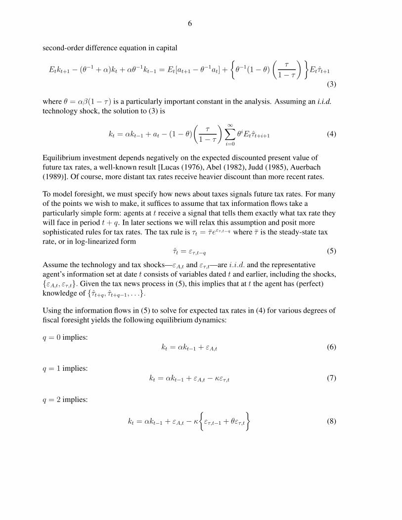
second-order difference equation in capital

Etkt+1 − (θ−1 + α)kt + αθ−1kt−1 = Et[at+1 − θ−1at] +

θ−1(1− θ)(

τ

1− τ

)

Etτt+1

(3)

where θ = αβ(1− τ ) is a particularly important constant in the analysis. Assuming an i.i.d.

technology shock, the solution to (3) is

kt = αkt−1 + at − (1− θ)(

τ

1− τ

) ∞∑

i=0

θiEtτt+i+1 (4)

Equilibrium investment depends negatively on the expected discounted present value of

future tax rates, a well-known result [Lucas (1976), Abel (1982), Judd (1985), Auerbach

(1989)]. Of course, more distant tax rates receive heavier discount than more recent rates.

To model foresight, we must specify how news about taxes signals future tax rates. For many

of the points we wish to make, it suffices to assume that tax information flows take a

particularly simple form: agents at t receive a signal that tells them exactly what tax rate they

will face in period t+ q. In later sections we will relax this assumption and posit more

sophisticated rules for tax rates. The tax rule is τt = τ eετ,t−q where τ is the steady-state tax

rate, or in log-linearized form

τt = ετ,t−q (5)

Assume the technology and tax shocks—εA,t and ετ,t—are i.i.d. and the representative

agent’s information set at date t consists of variables dated t and earlier, including the shocks,

εA,t, ετ,t. Given the tax news process in (5), this implies that at t the agent has (perfect)

knowledge of τt+q, τt+q−1, . . ..

Using the information flows in (5) to solve for expected tax rates in (4) for various degrees of

fiscal foresight yields the following equilibrium dynamics:

q = 0 implies:

kt = αkt−1 + εA,t (6)

q = 1 implies:

kt = αkt−1 + εA,t − κετ,t (7)

q = 2 implies:

kt = αkt−1 + εA,t − κ

ετ,t−1 + θετ,t

(8)

7

q = 3 implies:

kt = αkt−1 + εA,t − κ

ετ,t−2 + θετ,t−1 + θ2ετ,t

(9)

where κ = (1− θ)(τ/(1− τ )).

If there is no foresight, q = 0, we get the usual result that i.i.d. shocks to tax rates have no

effect on capital accumulation. When there is some degree of tax foresight (q > 0), rational

agents will adjust capital contemporaneously to yield the unusual result that even serially

uncorrelated tax hikes reduce capital accumulation. Fiscal foresight manifests in the

additional moving average terms present in the equilibrium representation, with the number

of moving average terms increasing in the foresight horizon.

A striking, though seemingly perverse, implication of (8) and (9) is that more recent news is

discounted (by θ = αβ(1− τ ) < 1) relative to older news. This is because with two-quarter

foresight, ετ,t−1 affects τt+1, while ετ,t affects τt+2, so the news that affects tax rates farther

into the future receives the heaviest discount. While tax rates are discounted in the usual way,

tax news is discounted in reverse order. This difference in discounting between tax rates and

tax news stems from optimizing behavior and underlies the econometric problems that

foresight creates.

A. The Econometrics of Foresight

The moving average terms that foresight produces pose challenges for econometric inference.

Conventional econometric analyses, such as those using identified vector autoregressions

(VARs), can draw erroneous conclusions. Errors arise because models with foresight may

imply that the information set of private agents is larger than the econometrician’s.

An econometrician who estimates an identified VAR seeks to condition on the same

information set as the economic agents in order to recover the structural shocks ετ,t−j∞j=0.

Typically, this is achieved by conditioning the VAR estimates on current and past

observables. Consider the univariate case of conditioning on current and past capital,

kt−j∞j=0, and suppose that agents have two quarters of foresight. Using lag operators (i.e.,

Lsxt = xt−s), (8) may be written as

(1− αL)kt = −κ(L+ θ)ετ,t (10)

Will the econometrician’s conditioning set, current and past capital, span the same space as

the agents’ current and past structural shocks?3 The answer depends on whether ετ,t−j∞j=0

3More specifically, the information sets are equivalent if the the Hilbert space generated by kt−j∞j=0 is

equivalent (in mean-square norm) to the Hilbert space generated by ετ,t−j∞j=0.

8

is fundamental for kt−j∞j=0, using the terminology of Rozanov (1967). Fundamentalness

requires the equilibrium process to be invertible in current and past kt, so that

[1− αL

1 + θ−1L

]

kt

is a convergent sequence. If |θ| > 1, this condition holds and kt−j∞j=0 spans the same space

as ετ,t−j∞j=0. But a unique saddlepath solution requires |θ| < 1. Therefore, ετ,t−j∞j=0 is

not fundamental for kt−j∞j=0.

To determine the econometrician’s information set, we derive the Wold representation for ktfrom the one-step-ahead forecast errors associated with predicting kt conditional only on its

past values.

This representation emerges from flipping the root of the moving average representation from

inside the unit circle to outside the unit circle using the Blaschke factor, [(L+ θ)/(1 + θL)][see Hansen and Sargent (1991b) or Lippi and Reichlin (1994)]. The Wold representation for

capital is

(1− αL)kt = −κ(L+ θ)

[1 + θL

L + θ

]

︸ ︷︷ ︸

[L+ θ

1 + θL

]

ετ,t︸ ︷︷ ︸

= −κ(1 + θL) ε∗τ,t

= −κ

θε∗τ,t−1 + ε∗τ,t

(11)

By observing current and past capital, the econometrician recovers current and past ε∗τ , rather

than the news that private agents observe, current and past ετ . The econometrician’s

innovations are the statistical shocks associated with estimating the autoregressive

representation; those shocks represent information that is mostly “old news” to the agents of

the economy. Fundamental shocks map into the econometrician’s shocks as

ε∗τ,t =

[L+ θ

1 + θL

]

ετ,t = (L + θ)∞∑

j=0

−θjετ,t−j

= θετ,t + (1− θ2)ετ,t−1 − θ(1− θ2)ετ,t−2 + θ2(1− θ2)ετ,t−3 + · · · (12)

This mapping shows that what the econometrician recovers as the tax innovation at time t,ε∗τ,t, is actually a discounted sum of the tax news observed by the agents at date t and earlier.

An econometrician who ignores foresight will discount the innovations incorrectly. In the

econometrician’s representation, yesterday’s innovation has less effect than today’s

innovation, as the terms θε∗τ,t−1 + ε∗τ,t in (11) show. Agents with foresight, in contrast,

discount news according to ετ,t−1 + θετ,t, as in (8), because yesterday’s news has a larger

effect on capital accumulation than today’s news. Differences in discounting patterns applied

by the econometrician and the agents lead to a variety of econometric problems.

9

By not modeling foresight, the econometrician has conditioned on a smaller information set.

The extent to which private agents condition on information that is not captured by current

and past variables in the econometrician’s information set determines the error associated

with the VAR. This error can be mapped directly into the θ parameter that governs the

non-invertibility of the equilibrium moving-average representation. The variance of the

one-step-ahead forecast error for the agent is

E[(kt+1 − E[kt+1|εt])2] = E

[(−κ(L+ θ)

1− αL ετ,t+1 − L−1[−κ(L+ θ)

1− αL + κθ]ετ,t

)2]

= (κθ)2σ2τ (13)

where εt denotes current and past ε. For the econometrician’s information set, the variance of

the forecast error is

E[(kt+1 − E[kt+1|kt])2] = E

[(−κ(L+ θ)

1− αL ετ,t+1 − L−1[−κ(1 + θL)

1− αL + κ]

[L + θ

1 + θL

]

ετ,t

)2]

= κ2σ2τ (14)

The ratio of (13) to (14) is θ2. As θ2 approaches unity (zero), the difference between the

agent’s and econometrician’s information sets gets smaller (larger). If θ is greater than or

equal to 1, the representation for capital becomes fundamental with respect to ετ,t and the

variances of the forecast errors in (13) and (14) coincide.

To examine the importance of the information discrepancies in this model, we plot impulse

response functions conditioning on the agents’ and econometrician’s information sets.

Impulse response functions are widely used to convey how agents respond to innovations, but

response functions based on the econometrician’s information set will not capture these

responses. Consider the impulse response functions generated by (8) and (11). Figure 1a

plots the responses of capital assuming two quarters of foresight (with

α = 0.36, β = 0.99, τ = 0.25, σ2τ = 1). With foresight, agents know exactly when the

innovation in fiscal policy translates into changes in the tax rate. This creates the sharp

decline in capital one quarter after the news arrives and before the tax rate changes, as the

dotted-dashed line indicates. The econometrician’s VAR, though, discounts the innovations

incorrectly and reports that the biggest decline in capital occurs on impact, suggesting that

foresight does not exist (solid line). The difference between the response functions can be

quite dramatic, especially at short horizons.

Figure 1a shows that the econometrician will infer that the tax shock is unanticipated. Of

course, not all shocks that affect fiscal policy are known several quarters in advance.

Consider a tax rate process, τt = euτ,t + ετ,t−q, that allows for both anticipated (ετ ) and

unanticipated (euτ ) shocks at time t. If these shocks are orthogonal at all leads and lags, then

the equilibrium dynamics of (3) will not change because i.i.d. tax shocks will not alter the

dynamics of capital. An econometrician who does not account for foresight will attribute all

of the dynamics associated with the anticipated component of the tax rate to the

unanticipated component. This suggests that researchers interested in the dynamic effects of

10

0 1 2 3 4 5 6 7 8−0.35

−0.3

−0.25

−0.2

−0.15

−0.1

−0.05

0

Agent

Econometrician

Figure 1a: Response of K with q = 2

0 1 2 3 4 5 6

−0.25

−0.2

−0.15

−0.1

−0.05

0

0.05

0.1

Agent

Econometrician

↑ σ2a = 1

← σ2a = 0.01

Figure 1b: Response of K for VAR (τt, kt)′

Figure 1. Responses of Capital to Tax Increase with α = 0.36, β = 0.99, τ = 0.25. Figure

1a plots the response of (13) and (14). Figure 1b plots the response to the VAR (τt, kt)′. Both

figures assume two quarters of foresight.

fiscal policy—whether the interest is in anticipated or unanticipated changes in policy—must

explicitly account for foresight to avoid spurious conclusions.

Conditioning on more variables will not always lead to better inference. In the case of

two-quarter foresight, suppose the econometrician estimates a VAR that includes the tax rate

and the capital stock as observables

[τtkt

]

=

[L2 0

−κ(L+θ)1−αL

11−αL

] [ετ,tεA,t

]

xt = H(L)εt (15)

A necessary condition for εt to be a fundamental for xt is that the determinant of H(z) be

analytic with no zeros inside the unit circle. Foresight creates a zero inside the unit circle (at

z = 0), implying that the information set generated by xt,xt−1,xt−2, ... is smaller than the

information set generated by εt, εt−1, εt−2, ....

The Wold representation for (15) is obtained by finding Blaschke matrices B(L) and

orthonormal matrices W , W that do not alter the covariance generating function of xt, but

“flip” the zeros outside of the unit circle. To do this we seek a B(L), W , and W that satisfy

B(L)B(L−1)′ = I and WW ′ = I , W W ′ = I , and produce innovations that span the space

generated by xt,xt−1,xt−2, .... The first step in the algorithm is to evaluate H(L) at L = 0,

and postmultiply by W so as to put the zeros in the first column of the product matrix

[Townsend (1983, appendix A)]. Remaining columns of W can be constructed from a

Gram-Schmidt orthogonalization procedure. The orthonormalW matrix ensures that the

representation remains causal, preserving the assumption that the econometrician does not

11

observe future values of the variables. Postmultiplying by B(L) flips the zero outside of the

unit circle. With two zeros inside the unit circle for (15), repeat this algorithm (find an

orthonormal matrix W that aligns the zeros in the first column, etc.). Proceeding in this

fashion delivers the representation

[τtkt

]

=

[L2 0

−k(L+θ)1−αL

11−αL

]

WB(L)WB(L)

︸ ︷︷ ︸

B(L−1)W ′B(L−1)W ′

[ετ,tεA,t

]

︸ ︷︷ ︸

xt = H∗(L) ε∗t (16)

where

W =

1√1+(θκ)2

−κθ√1+(θκ)2

κθ√1+(θκ)2

1√1+(θκ)2

, W =

[∆(1 + κ2θ2) −∆κ

∆κ ∆(1 + κ2θ2)

]

,B(L) =

[L−1 00 1

]

and ∆ = [(1 + κ2θ2)2 + κ2]−1/2.

Now the econometric problems are more severe. First, the econometrician who proceeds with

VAR analysis using (16) will likely obtain an impulse response function in which foresight

does not appear to exist in the data. Figure 1b depicts the response of capital to a tax increase

for the agent (dotted-dashed line) and econometrician as the variance of the technology shock

decreases from 1 to 0.01. Conditioning on the econometrician’s information set, the path of

capital is flat when σ2a = σ2

τ = 1. In theory, unanticipated i.i.d. capital tax shocks have no

effect on the economy, so based on the flat response of capital, an econometrician will infer

that the effects of fiscal policy are limited to unanticipated components only. By not

modeling foresight, the econometrician achieves a “self-fulfilling prophesy” and wrongly

concludes that foresight is not an issue.4

Second, as the variance of the tax shock increases relative to the technology shock, the errors

associated with foresight become more pronounced. Figure 1b shows that the initial response

of capital to a one-standard-deviation increase in the tax shock increases from 0 to 0.12 as σ2a

decreases from 1 to 0.01, so that an anticipated tax increase could be estimated to have no

effect or a positive effect on capital and output.

Existing empirical work reports a diverse set of inferences about the effects of an anticipated

tax increase on output. Figures 1a and 1b demonstrate that even this simple model can deliver

diverse results that depend on the underlying information flows.

4With this simple form of foresight, an econometrician who estimates a VAR in (τt+q , kt) will recover the true

shocks. But more sophisticated information flows, as in later sections, or empirically plausible tax rules, as inLeeper, Plante, and Traum (2010), preclude that easy fix.

12

Finally, all conditional statistics reported by the econometrician will be misspecified.

Consider the variance decompositions that Hansen and Sargent (1991b) emphasize. Let

E(xt − E∗t−jxt)(xt − E∗

t−jxt)′ =

j−1∑

k=0

H∗k Σ∗ H′∗

k

denote the j-step ahead prediction error variance associated with the econometrician’s

information set, where Σ∗ is the variance-covariance matrix associated with (ε∗τ,t, ε∗A,t)

′. Like

impulse response functions, variance decompositions are derived using conditional

expectations, so the discrepancy in the information sets implies that the coefficients

generated by H∗(L) will misallocate the variance across the structural shocks.5 Figure 1b

suggests that the econometrician will treat the tax shock as nearly i.i.d. and infer that none of

the variation in capital (and hence output) can be attributed to tax innovations; all of the

variation will be attributed to the technology shock. This inference holds even if, in fact, the

tax shock explained nearly all of the variation in capital (for example, when the variance of

the technology shock, σ2A, is arbitrarily small).

Further implications of foresight appear in the appendix, where we show that Granger

causality tests and tests of economic theory, such as tests of present value restrictions, will be

misspecified in the presence of foresight. Errors associated with ignoring foresight can be

quite large.

B. Generalizations

The previous example assumes an i.i.d. tax shock, but the difficulties associated with

foresight extend to more general setups. Suppose the stationary tax rate follows

τt = C(L)Lqετ,t, where C(L) is a polynomial in the lag operator L and q is the degree of

foresight. The only restriction placed on C(L) is that the corresponding coefficients are

square summable, which allows for any serial correlation pattern. Agents guess that the law

of motion for capital is given by a square summable linear combination of tax and technology

shocks, kt = F (L)ετ,t +G(L)εa,t, as Whiteman (1983) shows. Focusing on tax shocks only

and substituting this guess into the difference equation for capital in (3) yields

θL−1[F (L)− F0]ετ,t − (1 + αθ)F (L)ετ,t + αLF (L)ετ,t =

(1− θ)(

τ

1− τ

)

Et+1τt+1

where the Wiener-Kolmogorov formula is used to take expectations (i.e.,

Etxt+1 = L−1[D(L)−D0]εx,t), and θ = αβ(1− τ ). Uniqueness of the rational expectations

equilibrium requires |θ| < 1, where the equilibrium F (L)ετ,t for q degrees of foresight is

5This result holds even though the statistical shocks of the VAR remain uncorrelated. Orthogonality of the

Blaschke and W matrices (B(L)B(L−1) = I and WW ′ = WW ′ = I) implies that the unconditional second

moments of the VAR system remain the same, but the conditional moments will be different.

13

given by

F (L)ετ,t = −[κ[LqC(L)− θqC(θ)]

(1− αL)(L − θ)

]

ετ,t (17)

This equation makes plain how foresight impinges on optimal capital accumulation for any

choice of C(L). Whenever q ≥ 2, the equilibrium contains moving average components even

when C(L) is purely autoregressive. This representation suggests that it is straightforward to

construct impulse response functions that take a wide range of shapes (including

hump-shaped), for which the dynamic equation for capital continues to be non-invertible in

current and past kt. For example, setting C(L) = (1− ρ1L− ρ2L2)−1 and assuming two

quarters of foresight (q = 2) implies that the tax shocks ετ t are non-fundamental for kt if

θ < (1 + ρ1)−1. Because the condition for a non-fundamental moving average representation

is independent of ρ2, impulse response functions of non-fundamental moving average

representations can adopt many forms.

The logic that leads foresight to produce equilibria with non-fundamental moving-average

representations extends to a large class of models. Consider the generic multivariate rational

expectations model

Γ0yt = Γ1yt−1 + Ψzt + Πηt (18)

where yt is an n × 1 vector of endogenous variables, zt is an m× 1 vector of exogenous

random shocks, η is a k × 1 vector of expectation errors, which satisfy Etηt+1 = 0 for all t.Γ0 and Γ1 are n× n coefficient matrices, along with Ψ (n×m) and Π (n× k). Klein (2000)

and Sims (2002) use a generalized Schur decomposition of Γ0 and Γ1 to show that there exist

matrices such that Q′ΛZ ′ = Γ0, Q′ΩZ ′ = Γ1, Q′Q = Z ′Z = In×n, where Λ and Ω are

upper-triangular. The ratios of the diagonal elements of Ω and Λ, ωii/λii, are the generalized

eigenvalues. Defining wt = Z ′yt and pre-multiplying (18) by Q, yields the decomposition

[Λ11 Λ12

0 Λ22

][w1,t

w2,t

]

=

[Ω11 Ω12

0 Ω22

][w1,t−1

w2,t−1

]

+

[Q1

Q2

]

(Ψzt + Πηt) (19)

The system is partitioned so that the generalized eigenvalues imply an explosive path for w2,t.

Analogous to (4), w2,t must be solved forward to ensure stability of the system. Sims shows

that the forward solution of (18) is

yt = Θ1yt−1 + Θ0zt + ΘyΘz

∞∑

s=1

Θs−1f Etzt+s (20)

where Θf = Ω−122 Λ22 is the inverse of the unstable eigenvalues, and Θz = Ω−1

22 Q2Ψ. Θf is the

multivariate analog to θ in the simple analytical example and satisfies∑∞

j=0 tr ΘfΘ′

f <∞.6

6Mertens and Ravn (2010) derive this restriction in a real business cycle model with one unstable eigenvalue

and refer to Θf as the “anticipation rate” because it is the rate at which news or foresight is discounted. In line

with our findings, they argue that this relationship between the anticipation rate and unstable eigenvalues is a

robust feature of models with foresight.

14

If the structural shocks, zt, are i.i.d. and agents do not have foresight, then the last term in

(20) drops out of the solution and the equilibrium has a VAR representation. In this case,

conditioning on the control and state variables, yt, allows a VAR to recover the structural

shocks. But when agents have foresight, the equilibrium representation becomes a VARMA

with the MA coefficients Θf . Suppose the structural shocks are given by zt = εt−q, and

agents have foresight—at date t they observe ε’s dated t and earlier, then the equilibrium is

yt = Θ1yt−1 + Θ0εt−q + ΘyΘz[εt−q+1 + Θf εt−q+2 + · · ·+ Θq−1f εt]. (21)

As in the univariate case, the fiscal variables in (20), zt+s, are discounted in the usual way,

but the news innovations in (21), εt−q, are discounted perversely, with more recent news

discounted the heaviest. This is why models with foresight are more likely to deliver

non-fundamental equilibrium representations.

The yt vector contains endogenous variables, which, like capital in the simple analytical

model of section II, are typically forward looking. We established in the Wold representation

(15) that simply adding forward-looking variables to the VAR does not always resolve the

noninvertibility. In rational expectations models, variables like capital and consumption

respond contemporaneously to news about future tax rates, but (21) shows that the

contemporaneous response of these variables will be muted by the discount factor Θq−1f .

Most of the adjustment in variables to news occurs at future dates (in periods t+ q), rather

than contemporaneously (at t). To derive a fundamental VARMA representation, we need to

augment (21) with a variable whose representation does not suffer from the perverse

discounting. That variable’s largest response to news will occur contemporaneously and

news will be discounted in the usual way, as in (20). This makes the moving average part of

(21) invertible, ensuring the econometrician’s information set is consistent with the agents’.

The extent to which foresight leads to econometric errors depends on the underlying structure

of the economy and the nature of information flows. The next section examines this issue in

two canonical macro models.

III. QUANTITATIVE IMPORTANCE OF FORESIGHT

The information flows specification in (5) was chosen for its analytical convenience, not for

its plausibility. To assess the quantitative importance of foresight, this section generalizes

those flows to capture actual news processes and embeds the generalized specification in two

empirically motivated DSGE models. We show how the nature of information flows affects

the inference errors an econometrician can make by not modeling foresight. Quantitative

importance is summarized by dynamic tax multipliers, comparing those estimated by an

econometrician who fits an identified VAR to the true tax multipliers.

15

A. Modeling Information Flows

Rich information flows characterize the arrival and accumulation of news about tax changes,

but generally fall into two periods: between initial proposal and final enactment—or

rejection—of a new tax law (“inside lag”) and between enactment and when the law takes

effect (“outside lag”).7 During the inside lag, information and expectations evolve about the

likelihood and the precise form of proposed legislation. Sources of information that mark the

beginning of the inside lag can be formal—a president’s State of the Union speech—or

informal—a politician’s campaign pledges. And this early information may be confirmed or

contravened by subsequent actions.8 Outside lags arise whenever there is a delay between the

legislation’s passage and its implementation, as when tax changes are phased in. The two

types of lags differ in important ways. During the inside lag, anticipated taxes are uncertain;

news arrives regularly and induces agents to update their expectations. Agents are solving a

dynamic signal extraction problem in an attempt to decipher noise from news. During the

outside lag, the tax law has been adopted, no more news arrives, and agents have perfect

foresight about future tax rates.

Examples clarify the nature of information flows. The Economic Recovery Tax Act of 1981,

enacted in August 1981, phased in tax reductions through the beginning of 1984 to yield an

outside lag of 10 quarters. In announcing his candidacy for president in November 1979,

Ronald Reagan made clear that he intended to substantially lower taxes: “The key to

restoring the health of the economy lies in cutting taxes” [Reagan (1979)]. News about future

taxes then arrived throughout 1980, evolving with Reagan’s prospects of winning office. An

additional six months passed between President Reagan’s formal call for tax relief in

February 1981 and the legislation’s enactment. The inside lag associated with this tax change

is, arguably, five or more quarters, with the weights agents place on the bits of news changing

over time. Taken together, the two lags imply a foresight period of about four years.

Adjustments to Social Security taxes can entail extraordinarily long lags. The National

Commission on Social Security Reform was established in December 1981 to recommend

solutions to the System’s short- and long-term solvency problems. Its recommendations,

reported in January 1983, formed the basis for the Social Security Amendments of 1983,

which were enacted in April 1983. The Amendments phased in payroll tax increases

beginning in 1984 and extending to 1990. Although their inside lag may have been only a

few quarters, the Amendments’ outside lag is over six years. Other changes in Social

Security taxes had comparably long lags.

To model these intricacies, we generalize (5) with a specification of information flows about

tax rates that is flexible enough to capture both inside and outside lags. For labor taxes, we

7These labels date back to Friedman (1948), where we combine the “recognition” and “decision” lags to forminside lags and our outside lags refer to how long it takes legislation to change tax rates.

8Announcing their candidacies, both Ronald Reagan and George W. Bush made clear their intentions to cut

taxes, well over a year before they took office and formally proposed tax cuts. George H. W. Bush, in contrast,

pledged in his announcement speech, “I am not going to raise your taxes—period.” That was two-and-a-half

years before he called for a tax increase. See http://www.4president.org for these speeches.

16

posit

τLt = ρτLt−1 +

J∑

j=0

φj[σLεLτ,t−j + ξσKεKτ,t−j

](22)

where τLt is the labor tax rate, ξ permits labor and capital tax rates to be correlated, and the

ε’s are serially uncorrelated. We posit the best-case scenario for econometricians in that the

tax processes are exogenous: in this case, identification is straightforward in the absence of

foresight, ensuring that all errors arise solely from foresight.

As before, the sequence of innovations, εLτ,t−j, εKτ,t−j∞j=0, enter the agent’s information set

directly. We interpret the moving-average coefficients as weights, imposing that∑

j φj = 1.

Modeling information flows as moving average processes captures the idea that from quarter

to quarter news about taxes evolves randomly, and generalizes the “perfect foresight”

information structure. To see this more clearly, set J = 2, ξ = 0, ρ = 0, and σL = 1, so the

tax rule becomes

τLt = θεt + (1− θ)εt−1

where θ ∈ (0, 1). If θ = 0, then agents have perfect foresight because they observe τLt+1

perfectly. If θ = 1, then agents have no foresight and receive news only about the

contemporaneous tax rate. As θ moves smoothly from 1 to 0, agents receive more news about

next period’s tax rate.

Specification (22) embeds many of the information flows that appear in theoretical studies of

foresight, including Christiano, Ilut, Motto, and Rostagno (2008), Jaimovich and Rebelo

(2009), and Fujiwara, Hirose, and Shintani (2011) in the context of technology news; Ramey

(2011) for government spending news; Yang (2005) and Mertens and Ravn (2011) with

regard to tax news, and Schmitt-Grohe and Uribe (2008) for news about a variety of

variables. These studies set φj = 0 for all j except for φq = 1, where q is the period of

foresight.9 These specifications imply that once the news arrives, agents have q periods of

perfect foresight about the object being modeled. This may be an adequate assumption about

information flows that stem from outside lags, but they miss altogether the inside lags. Inside

lags are periods when agents are learning about how the future may play out. Tax policies

develop over time, from initial informal proposals to formal proposals, all the way through

the legislative process. The φj coefficients in (22) reflect how agents update their views about

taxes during the inside lags. Values of the φj’s describe how information flows differ from

period to period.

9Some studies allow the news shocks, εt−j , to be drawn from distinct distributions for each j, and set φj = 1for each relevant j [Schmitt-Grohe and Uribe (2008), Fujiwara, Hirose, and Shintani (2011), and Mertens andRavn (2011)]. The j = 0 shock is unanticipated, while the j > 0 shocks are anticipated given information at

time t.

17

B. Model Descriptions

We study a real business cycle model—closely related to Chari, Kehoe, and McGrattan

(2008)—and a new Keynesian model—similar to those in Smets and Wouters (2003,

2007)—but add distorting tax rates on capital and labor income. These models are

workhorses in the macroeconomics literature so we provide only brief descriptions here. The

appendix describes the models and estimation strategies thoroughly.

In the real business cycle (RBC) model, a representative agent maximizes time-separable

discounted utility over consumption and leisure. The agent supplies labor and capital to a

representative firm, which produces output according to a Cobb-Douglas technology. The

government chooses a set of fiscal variables to satisfy the flow budget constraint,

Gt + Zt = τLt wtlt + τKt rKt kt−1, where Gt is government consumption, and Zt is transfers.

Log-linearized government consumption policy follows an AR(1) process and lump-sum

transfers adjust to balance the government budget constraint each period.

Tax legislation adjusts labor and capital taxes following (22) and its analog for capital tax

rates. Yang (2005) estimates the correlation between tax rates at 0.5, implying the value of ξ.Since changes in individual income tax rates affect both labor income taxes and part of

capital income taxes, the two tax shocks are often correlated.

The new Keynesian (NK) model extends the RBC model to incorporate real and nominal

rigidities that have been shown to help fit macroeconomic data. It also models fiscal

financing by allowing spending to adjust to stabilize government debt. The NK model adds

external habit formation, differentiated labor types, a monopolistically competitive

intermediate goods sector, variable capital utilization, wage and price rigidities, and a

monetary authority that follows a Taylor-type rule for setting nominal interest rates. Tax

policies obey (22) and government spending policies follow the process

Xt = ρXXt−1 + γX sBt−1 + σXε

Xt , X ∈ G, Z (23)

where sBt−1 ≡ Bt−1

Yt−1is the debt-output ratio and γX < 0.

We estimate the NK model using Bayesian methods and U.S. quarterly data from 1984 to

2007. To conduct simulations, we fix parameters at the mode of the posterior distributions

(see table 1 in the appendix). For the RBC model, the structural parameters are calibrated to

the values used in the literature and standard deviations of the shocks are set to the values

estimated in the NK model. By calibrating one model to well known values and estimating

the other model, we aim to demonstrate that our findings are not dependent on whether

parameters are calibrated or estimated.

18

Process Lags Description Coefficients

I Inside 6 qtrs, smooth news φj = 16

, j = 1, 2, . . . , 6φ0 = φ7 = φ8 = 0

II Inside 6 qtrs, concentrated news φ1 = φ2 = φ3 = 0.05,φ4 = 0.25φ5 = φ6 = 0.3, φ0 = φ7 = φ8 = 0

III Outside 8-qtr phase-in φj = 0 j 6= 8φ8 = 1

IV Outside 2-qtr phase-in φj = 0, j 6= 2φ2 = 1

Table 1. Information Flow Processes. Coefficient settings in tax rule (22).

C. Information Flows and Estimation Bias

The Romers’ (2007; 2010) narrative analysis and Yang’s (2009) timeline of outside lags

associated with federal tax changes reveal two critical features of information flows about

taxes. First, the foresight horizon varies considerably from one piece of tax legislation to the

next. Second, most tax changes entail substantial inside and outside lags. The generalized

specification (22) can model these features of information flows; simple specifications like

(5) cannot.

We examine the implications of four alternative information flows in the two DSGE models.

The alternatives reflect the diversity of information flows that previous authors have

documented. With a maximum length of tax foresight of eight quarters, the four information

processes we employ appear in table 1.

Processes I and II model inside lags that differ in the intensity of information flows. In I, the

flows are smooth, so news over the previous six quarters receives equal weight. Tax laws that

make steady progress through the legislature and get implemented with little delay create

flows like I. Process II concentrates the news on lags four through six, with small weight on

recent news. Tax changes implemented with a lag of about one year, with only slight changes

in details in the periods immediately before implementation, generate flows like II.

The outside lags in processes III and IV closely resemble the information flows that other

authors posit [for example, Mertens and Ravn (2011), and Forni, Gambetti, and Sala (2011)].

These processes imply that agents have eight-quarter (III) or two-quarter (IV) perfect

foresight about tax changes. Perfect foresight precludes any further changes in legislation, so

these processes are exclusively about implementation delays or phased-in tax changes.10

Table 2 summarizes the actual and estimated output multipliers associated with a typical tax

change in the RBC and NK models. In this exercise, the agent knows the information process

and observes the actual εt’s. The econometrician, on the other hand, bases inference on a set

10Ideally, information flows would encompass both inside and outside lags, but such flows would take us outside

of a linear structure. For example, one could posit the flows for the inside lag and then, conditional on

legislation having been enacted, switch to the outside lag specification, a process that is inherently nonlinear.

19

of observables. We construct the innovations representation based on the econometrician’s

conditioning set and use the Kalman filter to back out the econometrician’s inferences about

the responses of output and taxes to a shock to the tax rate. For the RBC model, the

econometrician conditions on the labor tax rate, income tax revenue, output, and investment;

the conditioning set for the NK model adds government consumption, private consumption,

labor, government debt, inflation, and the nominal interest rate. Thus, the estimated VAR

contains several “forward-looking” variables. As a robustness check, we examined many

combinations of alternative conditioning variables and found results that are consistent with

those in table 2. We report biases as estimated less actual multipliers and biases as a

percentage of the actual multipliers. In the absence of foresight, the bias is always zero.

Several general findings emerge from the table. Biases can be very large—hundreds of

percent—and can change sign over time across both models. In both models, the biggest

errors arise from outside lags—information processes III and IV—which are the information

flows most frequently posited in work on foresight. Inside lags with moving-average

terms—processes I and II—produce smaller, though still sizeable errors. Information process

III, in which agents have two years of perfect foresight about tax rates, generates the largest

inference errors in both models. It also confounds dynamics: the econometrician estimates

that the strongest effect is contemporaneous, while the largest impact actually occurs two or

three years later, depending on the model.

In the RBC model, actual multipliers change sign—positive in the foresight period and

negative later—but estimated multipliers are uniformly negative. Frictions in the NK model

propagate errors, making short-/long-run distinctions less pronounced.11 In the frictionless

RBC model, biases dissipate over time.

A consistent finding across the two models is that for horizons of eight quarters and beyond,

the econometrician underestimates the multiplier. The lone exception is the NK model under

information process I. The discounting of the tax innovations that appears in (4) and (20)

explains this result. An agent with q quarters of foresight discounts the innovations so that

the ετ,t−q shock receives little discount relative to shocks dated t through t− q − 1. As in the

analytical model, this perverse discounting occurs because ετ,t−q informs about the

contemporaneous tax rate, τt, while shocks dated t through t− q − 1 inform about future tax

rates. An econometrician, who does not observe the true innovations, applies the

conventional discounting to the innovations in her information set, as in (11). This makes the

econometrician’s impulse response functions die out faster than the true impulse response

functions to yield the underestimates.

These findings establish two key points. First, failure to model fiscal foresight can produce

quantitatively important errors of inference in the canonical models used for macroeconomic

policy analysis. Second, the precise nature of information flows about news matters for the

pattern of inference errors. Getting the information flows “right” poses a substantial

challenge to DSGE modelers. We turn now to empirical approaches designed to address the

errors associated with foresight.

11This echoes Leeper and Walker’s (2011) results for foresight about technology.

20

Real Business Cycle Model

Info Process 0 qtr 4 qtrs 8 qtrs 12 qtrs 20 qtrs peak (qtr)

I actual 0.19 −1.14 −1.48 −1.11 −0.65 −1.71 (6)estimated −0.31 −1.35 −1.27 −0.97 −0.59 −1.57 (5)bias −0.50 −0.21 0.20 0.14 0.06% bias −263% −19% 14% 12% 8%

II actual 0.15 −0.54 −1.40 −1.05 −0.61 −1.62 (6)estimated −0.56 −1.46 −1.19 −0.91 −0.55 −1.48 (2)bias −0.71 −0.92 0.21 0.14 0.06% bias −473% −169% 15% 13% 9%

III actual 0.09 0.16 −1.51 −1.12 −0.64 −1.51 (8)estimated −1.44 −1.09 −0.82 −0.64 −0.39 −1.44 (0)bias −1.54 −1.24 0.69 0.49 0.25% bias −1641% −784% 46% 43% 39%

IV actual 0.16 −1.34 −1.00 −0.76 −0.45 −1.56 (2)estimated −1.41 −1.06 −0.81 −0.62 −0.38 −1.41 (0)bias −1.57 0.28 0.20 0.14 0.07% bias −962% 21% 20% 18% 16%

New Keynesian Model

Info Process 0 qrt 4 qtrs 8 qtrs 12 qtrs 20 qtrs peak (qtr)

I actual −0.08 −0.36 −0.48 −0.43 −0.24 −0.48 (8)estimated −0.07 −0.44 −0.57 −0.51 −0.28 −0.57 (8)bias 0.01 −0.09 −0.09 −0.08 −0.04% bias 11% −24% −20% −18% −18%

II actual −0.06 −0.27 −0.43 −0.40 −0.23 −0.43 (9)estimated −0.09 −0.37 −0.42 −0.37 −0.19 −0.42 (7)bias −0.03 −0.10 0.00 0.04 0.04% bias −51% −37% 1% 9% 19%

III actual −0.03 −0.12 −0.32 −0.37 −0.26 −0.37 (12)estimated −0.14 −0.10 −0.08 −0.06 −0.01 −0.14 (0)bias −0.11 0.01 0.24 0.32 0.25% bias −340% 13% 76% 85% 95%

IV actual −0.06 −0.30 −0.33 −0.28 −0.14 −0.33 (7)estimated −0.15 −0.24 −0.26 −0.22 −0.11 −0.26 (7)bias −0.08 0.07 0.07 0.06 0.04% bias −128% 22% 22% 22% 25%

Table 2. Output Multipliers for a Labor Tax Change, Correlated with a Capital Tax Change.

Multipliers are output responses scaled by the peak response of revenues, converted to dollars,

as in Blanchard and Perotti (2002). Agent knows the information process and observes the

actual εt’s. Econometrician bases inference on a set of observable variables, as described in

text. Biases equal estimated less actual multipliers.

IV. SOLVING THE PROBLEM

This section unifies the empirical lines of attack that appear in the literature to deal with the

econometric problems associated with foresight. We show how seemingly diverse

approaches—for example, the narrative methods of Romer and Romer (2010) and Ramey

(2011) and the dynamic stochastic general equilibrium approaches of Fujiwara, Hirose, and

Shintani (2011) and Schmitt-Grohe and Uribe (2008)—are closely related attempts to solve

the problems caused by foresight. Each approach aims to resolve a non-uniqueness problem

intrinsic to moving average representations. We briefly discuss three lines of attack.12

12Detailed calculations in support of the discussion in this section appear in the appendix.

21

A. An Organizing Principle

Moving average representations are not unique for two distinct reasons that Hansen and

Sargent (1991a) emphasize. Understanding the reasons for non-uniqueness provides a useful

way to characterization solutions to the problems that foresight creates. Consider the Wold

representation for the n× 1 vector stochastic process xt

xt =∞∑

j=0

H∗j ε

∗t−j (24)

where∑∞

j=0 tr H∗jH

∗′

j <∞ and ε∗t is an n-dimensional white noise process defined as the

innovation in predicting xt linearly from its semi-infinite past (ε∗t ≡ xt − P [xt|xt−1]).

Two transformations are observationally equivalent to (24). The first comes from multiplying

by a nonsingular matrix U ,

xt =∞∑

j=0

(H∗jU

−1)(Uε∗t−j) (25)

where the innovation is now defined as Uε∗t and H∗

jU−1 represents the altered impulse

responses. If U is nonsingular, then the new innovations process spans the same space as xt

and the information content of Uε∗t is identical to that of ε

∗t . This is the type of

non-uniqueness that Sims (1980) describes. Researchers confront this non-uniqueness with

different orthogonalization schemes that rotate the covariance matrix through recursive

orderings [Sims (1980)], short-run restrictions [Bernanke (1986), Sims (1986)], long-run

restrictions [Blanchard and Quah (1989)], a combination of short and long-run restrictions

[Galı (1999)], or sign restrictions [Faust (1998), Canova (2002), Uhlig (2005)].

Foresight produces a second type of non-uniqueness. It is also observationally equivalent to

(24), and is described by the non-fundamental representation

xt =∞∑

j=0

Hjεt−j (26)

where now εt−j∞j=0 spans a larger space than xt−j∞j=0, and H(L) satisfies

H∗(z)Eε∗t ε

∗′

t H∗(z−1)′ = H(z)Eεtε

′tH(z−1)′.

where H(z) denotes the z-transform [see, Sargent (1979)]. Under the typical assumption that

agents observe the structural shocks εt directly, while the econometrician observes only xt,

models with sufficient foresight belong to this class of non-fundamental representations. The

covariance generating functions of H(L)εt and H∗(L)ε∗t are identical, but only H∗(L)possesses an invertible representation in xt. Letting A(L) = H∗(L)−1, the typical VAR

22

methodology delivers

xt = A−10 [A1xt−1 + A2xt−2 + · · ·+ ε

∗t ]. (27)

Identifying A−10 in the usual way recovers the shocks ε

∗t , but not the structural shocks, εt, that

agents observe; the econometrician conditions on a smaller information set than do agents.

Hansen and Sargent’s non-uniqueness point sends a clear message: to identify structural

shocks in a vector autoregression, both types of non-uniqueness must be confronted.

Confronting the non-uniqueness in (25) does not solve the non-uniqueness of representation

(26), and vice versa. A large literature focuses on the non-uniqueness associated with (25).

Identifying (26), though, receives less attention and requires the econometrician to condition

on the same information set as the agents they are modeling.

B. Lines of Attack

Casting the problem as resolving the two distinct forms of non-uniqueness sheds light on

three approaches that appear in the empirical macro literature. One line of attack estimates

conventional VARs, identified in a variety of creative ways to isolate anticipated effects, and

then examines the impacts of foresight [Sims (1988), Blanchard and Perotti (2002), Yang

(2007), Mountford and Uhlig (2009), Beaudry and Portier (2006), Fisher and Peters (2010),

Barsky and Sims (2011)]. For example, Beaudry and Portier (2006) and Fisher and Peters

(2010) condition on stock prices to capture news about expected changes in technology and

government spending, respectively. Barsky and Sims (2011) identify news about productivity

as the shock that is orthogonal to current utilization-adjusted productivity that best explains

future variations in adjusted productivity.

A second line of attack argues that conventional VARs cannot adequately measure the

impacts of foreseen changes in fiscal policy and pursues a narrative approach that introduces

new information to aid identification [Ramey and Shapiro (1998), Edelberg, Eichenbaum,

and Fisher (1999), Burnside, Eichenbaum, and Fisher (2004), Ramey (2011), Romer and

Romer (2010)]. A third approach uses standard methods to estimate a model with foresight.

To execute these methods, Schmitt-Grohe and Uribe (2008) and Fujiwara, Hirose, and

Shintani (2011) make very particular assumptions about the information flows that give rise

to foresight about technology and government spending. The tradeoff is that the modeler

must be explicit about the role of information in the economy. Each line of attack tries to

align agents’ and the econometrician’s information sets to address the second type of

non-uniqueness that (26) describes.

1. The Narrative Approach

Narrative approaches to fiscal policy—pioneered by Ramey and Shapiro (1998), Romer and

Romer (2010), Ramey (2011), and Mertens and Ravn (2011)—expands the econometrician’s

information set by using fresh data sources to identify fiscal news. For example, Ramey

23

(2011) derives a direct measure of spending news by culling from Business Week dates when

there were significant increases in the expected present value of military spending. To the

extent that this fiscal news is triggered by non-economic factors, it may be treated as

exogenous for inferring the impacts of news on macroeconomic time series. Ramey

augments the econometrician’s usual information set by adding this news to fiscal VARs and

infers that anticipated expansions in federal government spending reduce most measures of

consumption and real wages, a strikingly non-Keynesian finding.

Recognizing the intrinsic endogeneity of tax policy decisions, Romer and Romer (2010)

compile a data series on the forecasted revenue consequences of federal tax changes since

World War II. Romer and Romer identify as “exogenous” those revenue changes that were a

response to concerns about long-run economic growth or about the state of government debt.

Using this measure of tax news, Mertens and Ravn (2011) apply a timing convention to

distinguish between unanticipated and anticipated news. They append tax news as exogenous

regressors to a VAR with a time trend

Xt = A +Bt+ C(L)Xt−1 +D(L)T ut + F (L)T at,0 +K∑

i=1

GiTat,i + et (28)

where X is a vector of macro time series, D(L)T ut + F (L)T at,0 reflects dependence on current

past unanticipated and anticipated news, and∑K

i=1GiTat,i yields the impacts of known, but

not-yet-implemented tax changes. Mertens and Ravn obtain provocative results: anticipated

tax cuts induce sharp economic slowdowns during the period of foresight, and may even

produce recessions.

Narrative approaches face two criticisms. First, theoretical and empirical models often do not

line up in their treatments of information flows. Romer and Romer (2007, 2010) base their

tax-shock series on narrative sources that report both enacted and proposed tax changes, but

Mertens and Ravn’s (2011) theory treats all anticipated tax changes as stemming from

outside lags. The Romers also limit themselves to actions that actually change tax liabilities,

so their data series excludes proposals that do not reach fruition, while news specifications

like those in section III allow for revisions in expectations when proposals fail. Ramey’s

(2009a; 2011) narrative analysis identifies a number of instances where the news about major

military build ups arrived well before any explicit legislative actions were taken, which are

clear examples of inside lags. But Ramey’s (2009b) theoretical specification posits a military

spending rule as an autoregressive process with a news shock lagged two periods, capturing

only the outside lag. This misalignment of information flows loosens the connection between

theory and empirics and muddies the interpretations of empirical findings.

Second, empirical implementations of narrative news variables typically treat news as

exogenous. Stock and Watson (2012) observe that, more precisely, narrative measures are

instruments for exogenous shocks. Their dynamic factor analysis uncovers some unsettling

characteristics of the fiscal news series derived by Romer and Romer (2010), Fisher and

Peters (2010), and Ramey (2011). First, the fiscal instruments are weak, suggesting they are

24

only weakly correlated with the underlying fiscal news shocks.13 Second, the Romer-Romer

tax series is highly correlated (0.93) with the Fisher-Peters government spending series,

making it difficult to interpret the two shocks as distinct fiscal actions. Finally, all three fiscal

news measures are highly correlated with monetary policy shocks, raising doubts about the

efficacy of identifying one type of macro policy independently of the other.14

2. Conditioning on Asset Prices

If asset markets are efficient, the information contained in asset prices should coincide with

all available information to agents and adding asset prices to a VAR should help align the

information sets of the econometrician and agent. With respect to fiscal foresight, there is an

asset class that is particularly useful for isolating news about future tax shocks. In the United

States, municipal bonds are exempt from federal taxes and the differential tax treatment of

municipal and treasury bonds can help identify news about tax changes.15 If YMt is the yield

on a municipal bond at t and Yt is the yield on a taxable bond, and assuming the bonds have

the same term to maturity, callability, market risk, credit risk, and so forth, then an “implicit

tax rate” is given by τ It = 1− YMt /Yt. This is the tax rate at which investors are indifferent

between tax-exempt and taxable bonds. With forward-looking bond traders, the implicit tax

rate predicts subsequent movements in individual tax rates: if investors expect individual tax

rates to rise (fall), they drive up (down) yields on taxable bonds until they are indifferent

between taxable and nontaxable bonds.16

More precisely, a newly issued tax-exempt bond with maturity T , a par value of $1, and

per-period coupon payments CM , will sell at par if

1 =CM

∑Tt=1(1 +Rτ

t )t+

1

(1 +RτT )T

, (29)

where Rτt is the after-tax nominal interest rate for payments made in period t. No-arbitrage

conditions imply that an identical taxable bond paying coupon C , and selling at par satisfies

1 =

∑Tt=1C(1− τ et )

∑Tt=1(1 +Rτ

t )t

+1

(1 +RτT )T

, (30)

where τ et is the future tax rate expected to hold in period t.

13Weak instrument may also be a sign of endogeneity problems.

14Of course, Stock and Watson’s findings are conditional on the variables they include in their factor model and

on the labels they choose to attach to the six factors they isolate.

15Depending on the type of bond, municipal bonds can also be exempt from the Alternative Minimum Tax, state,

and local taxes. Ang, Bhansali, and Xing (2010) describe the municipal bond market.

16There is a large literature demonstrating the ability of the municipal bond market to forecast changes in fiscalpolicy [Poterba (1989), Fortune (1996), Park (1997a), Kueng (2011)].

25

Bonds that sell at par have a yield-to-maturity that equals the coupon payments, so the

implicit tax rate is τ IT = 1− CM/C . Subtracting (III.2) from (III.1) and solving for CM/Cgives

τ IT =T∑

t=1

ωtτet , (31)

where ωt = δt/∑T

t=1 δt and δt = (1 +Rτt )

−t. The current implicit tax rate is a weighted

average of discounted expected future tax rates from t = 1 to T and should respond

immediately to news about anticipated future tax changes.

Equation (III.3) reveals the advantages of using municipal bond spreads to capture

information flows about pending tax changes. First, there is no need to specify a priori the

period of foresight. Under efficient markets, the implicit tax rate reflects the extent to which

agents do or do not have foresight. Second, there is no need to specify a functional form for

information flows. In section III, we modeled information flows as one of several possible

information processes. We would have to conduct a similar sensitivity analysis if we were

estimating a DSGE model. Using the implicit tax rate avoids taking an a priori stand on the

nature of information flows. Finally, conditioning on the implicit tax rate resolves the

non-uniqueness associated with moving-average representation (26). Like the capital

accumulation equation in section II, the implicit tax rate depends on the discounted future

path of taxes. Unlike the capital equation, the yield curve of municipal bonds isolates the

about taxes at different horizons.17

Employing exactly the identification scheme and data set of Blanchard and Perotti (2002)

(BP), we ask how augmenting the econometrician’s information set with a direct measure of

tax news affects inferences.18 To conserve space, we report the data construction and

estimation procedure in Leeper, Walker, and Yang (2011) and the appendix. We find that

municipal bonds respond to news about tax policy and that implicit tax rates are

Granger-causally prior relative to the information sets in the fiscal VAR system that

Blanchard and Perotti (2002) estimate.

Adding implicit tax rates dramatically changes the VAR results of BP: anticipated tax

increases raise output substantially for about three years before output begins to decline.

This contrasts sharply to the anemic response of output to an anticipated tax shock in BP

(Figure III, p. 1343), which led them to conclude, “there is not much evidence of an effect of

anticipated tax changes on output [p. 1353].” The difference in the results can be attributed to

how fiscal foresight is identified. By conditioning on one- and five-year municipal bond yield

17As an oversimplified example, suppose that agents have two quarters of foresight and the econometrician has

access to the implicit tax rate with maturities of one and two quarters. The one-quarter implicit tax rate

identifies one-quarter news, while the difference between the implicit tax rates identifies two-quarter news.

18We do the same exercise for Mountford and Uhlig (2009). While the results are not as striking as for BP, wedo find that conditioning on implicit tax rates qualitatively alters the findings of Mountford-Uhlig. For example,

investment multipliers, which Mountford-Uhlig estimated to be zero, become significantly positive. See Leeper,

Walker, and Yang (2011) and the appendix for more details.

26

spreads, we allow for a much longer foresight horizon than the BP approach, which assumes

agents have only one-quarter of foresight. These differences underscore the importance of

modeling information flows.

Our finding that news of higher taxes increases economic activity over much of the

anticipation period echoes results from two very different methodologies. In a case study,

House and Shapiro (2006) argue that the phased-in tax reductions enacted by the 2001

Economic Growth and Tax Relief Reconciliation Act played a significant role in creating the

unusually slow recovery from the 2001 recession. By feeding the legislated paths of marginal

tax rates on labor and capital into an RBC model, the authors generate a path of equilibrium

GDP that declines in response to an anticipated tax reduction. Our results are also consistent

with Mertens and Ravn (2011) whose augmented VAR, (28), implies that an anticipated tax

increase induces a boom in output whose amplitude and duration increase with the period of

foresight. In contrast to our approach with muni-treasury spreads, Mertens and Ravn must

specify a priori the period of foresight and maintain that anticipated taxes are

exogenous—assumptions that are critical to the quantitative effects they obtain. Nonetheless,

the qualitative effects closely resemble our results.

There are obvious limitations to using municipal bonds as a measure of anticipated tax

changes. First, fiscal news must be separated from other factors that influence municipal

bonds (callability, liquidity risk, default risk, etc.), factors whose influence can be controlled

for and limited by using high-quality municipal bond data. Leeper, Richter, and Walker

(2011) show how to construct a risk-adjusted implicit tax rate based on the methodology of

Fortune (1996). They argue that for AAA-rated municipal bonds, the risk adjustment is not

substantial. Using state municipal bonds, Kueng (2011) shows that default risk and liquidity

factors are nearly negligible for maturities of longer horizons and that municipal bonds

contain substantial news about pending tax changes. Second, the marginal investor may be

high-income households and not representative of the typical taxpayer. Kueng (2011)

provides supporting evidence but argues that it does not invalidate using municipal bonds to

back out news about pending tax changes for other tax brackets because the economic

response to tax news depends on the path of expected taxes, not the level. If municipal bonds

provide an accurate indication of this path, the levels are irrelevant. Third, municipal bonds

respond to changes in individual income taxes only. While this is true, often changes to the

tax code (personal, corporate, etc.) occur simultaneously, so municipal bonds may not

accurate indicate how corporate taxes change, but they will can indicate when corporate taxes

will change. Finally, municipal bonds are an asset that is unique to the United States, which

limits the implementability of this approach.

3. Direct Estimation of DSGE Model

A third approach uses standard econometric methods, such as An and Schorfheide (2007), to

estimate a DSGE model in which agents have foresight about shocks that hit the economy.

Specifying the entire structure of the economy, including the information sets of the agents,

yields a likelihood function that contains sufficient information to overcome the

27

non-uniqueness of section A. In models with foresight, the likelihood will be an vector

ARMA process similar to the equilibrium processes of section II. When estimating the model

directly (via maximum likelihood or Bayesian techniques), one does not need to put the

equilibrium into VAR form and therefore the invertibility of the moving average process is

irrelevant. By defining the information sets explicitly, it is no longer critical whether the MA

representation is fundamental or non-fundamental because the likelihood function can

distinguish between the two.

This benefit comes at a cost. Modelers must make very particular assumptions about the

information flows that give rise to foresight about technology, government spending, taxes,

and so forth. Solutions are conditional on the specified information flows, aspects of the

economic structure about which economists rarely have well developed prior beliefs or direct

empirical evidence.19 For example, in models with foresight, the length of foresight (the q in

section III) and the strength of foresight (the MA coefficients, θ, in section III) must be

specified prior to estimation. As shown in table 2, the dynamic properties of the equilibria

can vary dramatically conditional on the news process.

Leeper and Walker (2011) argue that the information sets specified to achieve identification

in this regard are chosen largely arbitrarily, grounded in neither theory nor empirics.

Alternative, equally plausible processes for news, can deliver strikingly different equilibrium

dynamics. Surprisingly, despite the centrality of information structures to the burgeoning

news literature, there has been essentially no exploration of alternative, equally plausible,

assumptions about how information about critical economic variables flows to agents.

V. CONCLUDING REMARKS

We have shown how foresight introduces econometric difficulties that complicate the

interpretation of conventional econometric analyses. Foresight, of any type, can introduce

non-fundamental moving average terms into the linear equilibrium process, changing the

mapping between the true news that agents observe and the “shocks” that the econometrician

identifies. Many of the econometric techniques in macroeconomists’ toolboxes can be

distorted by empirical methods that do not adequately estimate the non-invertible moving

average components of equilibrium time series. Section II uses simple analytics to describe

the nature of the problem. Section III demonstrates that failing to model foresight can

produce quantitatively important inference errors in data generated by models now in wide

use for macro policy analysis. Section IV explains that existing empirical methods to handle

foresight aim to resolve the same non-uniqueness, but in different ways.

This paper focuses on tax policy as a particularly relevant and tangible form of foresight.

There is little doubt that agents know and react to tax changes before they are implemented.

But the econometric difficulties that fiscal foresight creates are entirely general: they emerge

19That the assumptions about information flows matter to inferences from estimated DSGE models is shown intwo versions of the same paper that differ in information flow specifications and yield different inferences about

the relative importance of various shocks [Schmitt-Grohe and Uribe (2008, 2011)].

28

anytime agents respond to news about future realizations of fundamentals. Although the

problem is general, we suspect the solution is not. A general solution, if one exists, lies in the

future.

Foresight poses a challenging mix of structural and measurement problems. Hypothesized

information flows that are uninformed by observations and information sets that are

unrestricted by theory are unlikely to resolve the foresight problem. Answers lie in blending

theory with measurement.

29 APPENDIX I

APPENDIX I. SIMULATIONS DETAILS

A. Specifications of Models

For the quantitative results reported in section 3, we augment a prototype RBC model

(similar to the one in Chari, Kehoe, and McGrattan (2008)) and a standard New Keynesian

model (similar to those in Smets and Wouters (2003, 2007)) with distorting taxes levied on

capital and labor income. Agents in the models have foresight over tax policy changes. This

appendix describes the models and the calibration/estimation strategy. Except for the

parameters that characterize the information flow processes in the tax rules, the parameters in

the RBC model are calibrated to the values commonly used in the literature, and the NK

model is calibrated to the posterior mode of an estimated New Keynesian model, fit to U.S.

quarterly data from 1984 to 2007.

1. RBC Model

The representative agent maximizes utility

Et

∞∑

t=0

βt [log ct + φ log (1− lt)]

over consumption ct and labor lt, where β is the discount factor and φ is the preference

weight on leisure. The agent’s budget constraint is

ct + kt − (1− δ) kt−1 =(1− τLt

)wtlt +

(1− τKt

)rKt kt−1 + zt, where kt is capital, wt is the

wage rate, rKt is the real rate of return on capital, zt is government transfers, and δ is the

capital depreciation rate.

The representative firm produces output using the technology yt = uat kαt−1l

1−αt , where yt is

output and uat is total factor productivity, which follows the exogenous process

lnuat = ρa lnuat−1 + σaεat and εat ∼ N(0, 1). The firm chooses capital and labor to maximize

profit: yt − rKt kt−1 −wtlt.

Let capital letters denote aggregate quantities. Each period the government chooses a set of

fiscal variables to satisfy its budget constraint, Gt + Zt = τLt wtLt + τKt rKt Kt−1, where Gt is

government consumption. The goods market clearing condition is Yt = Ct + It +Gt, where

It = Kt − (1− δ)Kt−1 is investment.

Capital and labor tax rates follow the policy rules described by (22) and its capital tax analog.

30 APPENDIX I

2. New Keynesian Model

The NK model expands the RBC model to incorporate a variety of real and nominal frictions.

The economy is populated by a continuum of households, indexed by j ∈ [0, 1]. Each

household maximizes expected utility,

Et

∞∑

t=0

βtubt

[

(ct(j)− hCt−1)1−γ − 1

1− γ − lt(j)1+κ

1 + κ

]

where ubt is a general preference shock that follows the process ln(ubt) = ρb ln(ubt−1) + σbεbt .

We assume external habits that depend on aggregate consumption last period, Ct−1. As in

Erceg, Henderson, and Levin (2000), each household supplies unique labor inputs. A

state-contingent claim xt sold at a price of qt exists to eliminate the income differentials due

to differentiated labor. The household’s flow budget constraint (dropping index j) in units of

goods is

(1−τLt )Wt

Ptlt+(1−τKt )

RKt vtkt−1

Pt+Rt−1bt−1 + xt−1

πt+zt+dt = ct+it+bt+qtxt+Ψ(vt) kt−1

where Wt is the nominal wage rate, Pt is the general price level, and πt ≡ Pt

Pt−1is the inflation

rate. The model has variable capital utilization with the utilization rate vt; in the steady state,

v = 1. Varying the utilization rate involves a cost Ψ(vt) kt−1, where Ψ is an increasing,

convex function with Ψ(1) = 0. We define the utilization cost parameter ψ such that1−ψψ

= Ψ′′(1)Ψ′(1)

. The nominal rental rate for effective capital, vtkt−1, is RKt . it is investment

inclusive of adjustment costs. Capital evolves as kt = (1− δ)kt−1 +[

1− s(ui

titit−1

)]

× it,where s(·) is the adjustment cost function for investment; in the steady state,

s(1) = s′ (1) = 0, and s′′ (1) ≡ s > 0. Adjustment costs are subject to an investment shock,

uit, which follows the process ln(uit) = ρi ln(uit−1) + σiεit. Finally, each household owns an

equal share of all intermediate goods producing firms and receives dividends, dt.

Wages are rigid. A perfectly competitive labor packer purchases the differentiated labor

inputs and assembles them to form composite labor service, Lt, using the technology

Lt =[∫ 1

0lt (j)

11+ηw

t dj]1+ηw

t

, where ηwt denotes wage markups and is assumed to follow the

process ln(ηwt ) = ρw ln(ηwt−1) + σwεwt . The aggregate wage is Wt =

[∫ 1

0Wt (j)

1ηwt dj

]ηwt

.

Each period household j receives a signal to reset its nominal wage with a probability

1− ωw. Those who cannot reoptimize instead index their wages to past inflation according to

Wt (j) = Wt−1 (j)πχw

t−1.

Prices are rigid. A perfectly competitive final goods producer uses a continuum of

intermediate goods (yt(i), i ∈ [0, 1]) to produce the final good, Yt, using the technology[∫ 1

0yt(i)

1

1+ηpt di

]1+ηpt

≥ Yt. ηpt is the price markup for intermediate goods and follows the

process ln(ηpt ) = ρp ln(ηpt−1) + σpεpt . Intermediate goods producers are monopolistic

31 APPENDIX I

competitors in the product market. Firm i produces with the technology

yt = uat (vtkt−1)α(lt)

1−α, where uat is the total factor productivity, following the process

ln(uat ) = ρa ln(uat−1) + σaεat . Analogous to households’ wage decisions, a monopolistically

competitive intermediate firm faces a probability 1− ωp that is will be able to reset its

optimal price. Firms that cannot reoptimize index their prices to past inflation according to

pt(i) = pt−1(i)πχp

t−1. The goods market clearing condition is Yt = Ct + It +Gt +Ψ(vt)Kt−1.

The monetary authority obeys a rule that sets the nominal interest rate

Rt = ρrRt−1 + (1− ρr)(

φππt + φyYt

)

+ φdy

(

Yt − Yt−1

)

+ σmεmt

Fiscal policy evolves according to the rules in (22). The flow budget constraint of the

government is Bt + τKtRK

t

PtvtKt−1 + τLt

Wt

PtLt = Rt−1Bt−1

πt+Gt + Zt.

B. Calibration and Estimation

The RBC model is calibrated to values in the literature (largely following those in Chari,

Kehoe, and McGrattan (2008)): β = 0.99, φ = 1.6 implying a steady-state labor share of

0.32, α = 0.36, GY

= 0.2, and δ = 0.025. The steady-state capital and labor tax rates are set at

their sample means in the U.S. data from 1984 to 2007. The standard deviations of the

technology, transfer, and capital and labor tax shocks are calibrated to the estimated posterior

modes for the same shocks in the NK model to be described next (see table 3).

We estimate most of the parameters in the NK model using Bayesian methods, assuming

agents have no foresight over taxes. In the exercises, the model parameters are fixed at the

posterior modes that table 3 reports.

The NK model is log-linearized and solved by Sims’s (2002) method. Models have no

growth; data are detrended with a linear trend, as in Smets and Wouters (2003). The sample

period, 1984-2007, is selected because monetary policy is widely believed to follow a Taylor

rule [Taylor (1993)]. The estimation uses ten observables: real consumption, investment,

labor, wage rate, the nominal interest rate, inflation, capital tax revenues, labor tax revenues,

the sum of real government consumption and investment, and government transfers.

Government data include all federal, state, and local levels. Section C below describes the

data.

Several parameters, which are known to be difficult to estimate from the data, are calibrated.

The discount factor β is set to 0.99, implying an annual steady-state real interest rate of 4

percent. The capital income share in output is α = 0.36. The quarterly depreciation rate

δ = 0.025. The steady-state elasticity of substitution in the goods and labor markets ( 1+ηp

ηp ,1+ηw

ηw ) are assumed to be 8, which implies the steady-state markups in the product and labor

markets are approximately 14 percent, consistent with evidence that the average price

markup of U.S. firms is between 5-15 percent [Basu and Fernald (1995)]. Steady state (gross)

32 APPENDIX I

inflation is assumed to be 1. Other calibrated parameters are steady-state fiscal variables,

which are set to their sample means. Steady-state ratios of government spending and debt to

output come from their sample means: GY

= 0.17 and sb = 1.58 (debt to quarterly output),

where output is the sum of consumption, investment, and government spending. The

steady-state capital and labor income tax rates are computed based on Jones’s (2002)

definition: τK = 0.36 and τL = 0.24. When estimating the model, the correlation parameter

of capital and labor tax shocks ξ is assumed to be zero. The simulation results in table 2

assumes ξ = 0.26, implying a correlation of 0.5 between capital and labor tax shocks as

estimated by Yang (2005).

We assume that parameters are drawn independently and restrict the parameter space to

deliver a unique rational expectations equilibrium. Our priors follow closely the priors used

in Smets and Wouters (2007) for most of the shared parameters (see table 3). Priors for the

debt financing parameters (γg and γz) are guided by their implied dynamics. When γg and γzare too high, macro variables oscillate because the government overreacts to stabilize debt.

On the other hand, when the parameters are too small, a solution does not exist when

monetary policy is active (in the sense of Leeper (1991)). Priors for γg and γz have

independent normal distributions with means of 0.15 and standard deviations of 0.05.

To search for the posterior mode, the log-posterior function is minimized by Christopher

Sims’s minimization routine, csminwel. We initiate the mode search from different points,

and multiple modes do not appear to be a concern. Table 3 summarizes our estimation results

and compares them with the estimates by Smets and Wouters (2007) over a similar sample

period. For structural and monetary policy parameters, most of our estimates are comparable

to theirs.

C. Data Description

This section describes the data for estimating the NK model and the municipal and treasury

bonds data used in section 3.

1. Data for Estimating the New Keynesian Model

Unless otherwise noted, data are from the National Income and Product Accounts Tables

released by the Bureau of Economic Analysis.20 All data in levels are nominal values. To

convert nominal values to real per capita values, we deflate by the deflator for personal

consumption expenditures (Table 1.1.9, line 2) and a population index (described below).

Consumption. Consumption, C , is defined as total personal consumption expenditures

(Table 1.1.5, line 2).

20Further information on data construction appears in Traum and Yang (2010).

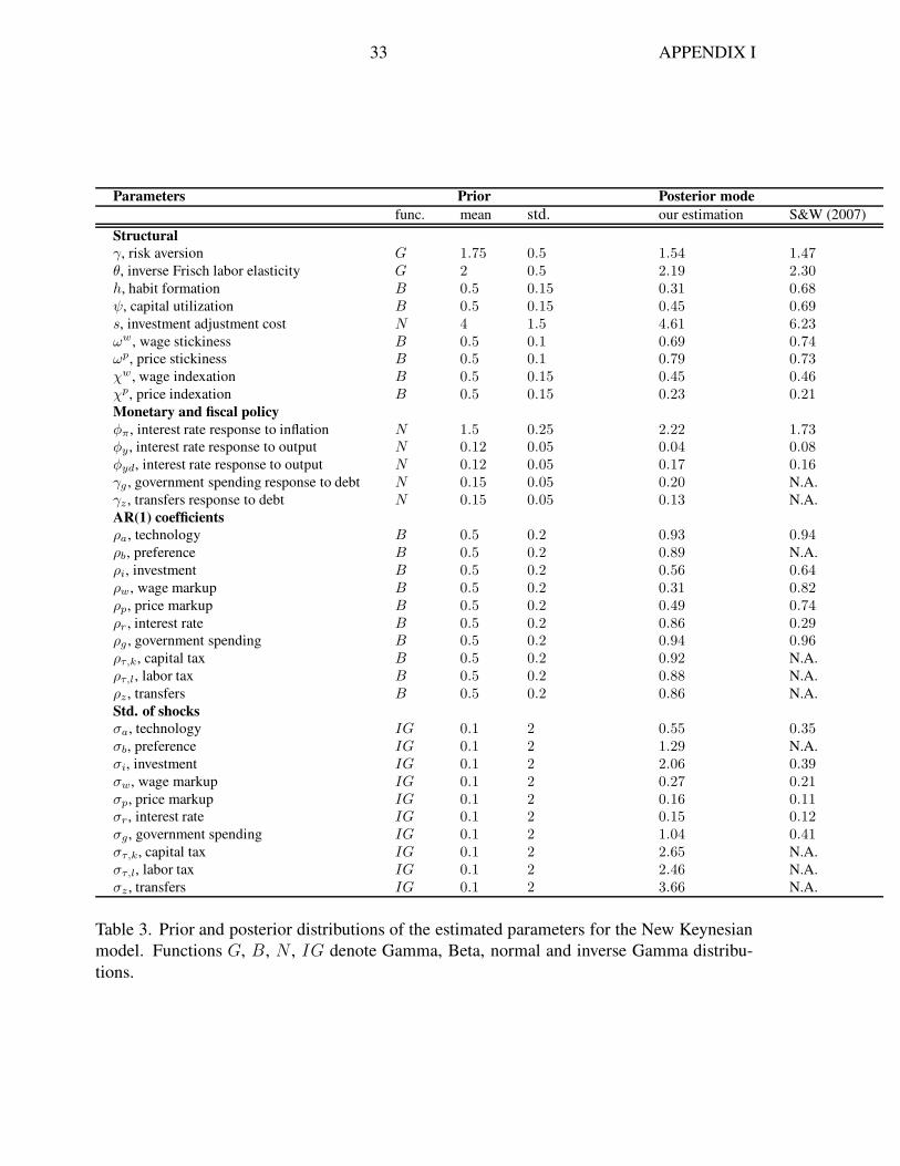
33 APPENDIX I

Parameters Prior Posterior mode

func. mean std. our estimation S&W (2007)

Structural

γ, risk aversion G 1.75 0.5 1.54 1.47θ, inverse Frisch labor elasticity G 2 0.5 2.19 2.30h, habit formation B 0.5 0.15 0.31 0.68ψ, capital utilization B 0.5 0.15 0.45 0.69s, investment adjustment cost N 4 1.5 4.61 6.23ωw, wage stickiness B 0.5 0.1 0.69 0.74ωp, price stickiness B 0.5 0.1 0.79 0.73χw, wage indexation B 0.5 0.15 0.45 0.46χp, price indexation B 0.5 0.15 0.23 0.21Monetary and fiscal policy

φπ, interest rate response to inflation N 1.5 0.25 2.22 1.73φy , interest rate response to output N 0.12 0.05 0.04 0.08φyd, interest rate response to output N 0.12 0.05 0.17 0.16γg , government spending response to debt N 0.15 0.05 0.20 N.A.

γz , transfers response to debt N 0.15 0.05 0.13 N.A.

AR(1) coefficients

ρa, technology B 0.5 0.2 0.93 0.94ρb, preference B 0.5 0.2 0.89 N.A.

ρi, investment B 0.5 0.2 0.56 0.64ρw, wage markup B 0.5 0.2 0.31 0.82ρp, price markup B 0.5 0.2 0.49 0.74ρr , interest rate B 0.5 0.2 0.86 0.29ρg , government spending B 0.5 0.2 0.94 0.96ρτ,k, capital tax B 0.5 0.2 0.92 N.A.

ρτ,l, labor tax B 0.5 0.2 0.88 N.A.

ρz , transfers B 0.5 0.2 0.86 N.A.

Std. of shocks

σa, technology IG 0.1 2 0.55 0.35σb, preference IG 0.1 2 1.29 N.A.

σi, investment IG 0.1 2 2.06 0.39σw, wage markup IG 0.1 2 0.27 0.21σp, price markup IG 0.1 2 0.16 0.11σr, interest rate IG 0.1 2 0.15 0.12σg, government spending IG 0.1 2 1.04 0.41στ,k, capital tax IG 0.1 2 2.65 N.A.

στ,l, labor tax IG 0.1 2 2.46 N.A.

σz , transfers IG 0.1 2 3.66 N.A.

Table 3. Prior and posterior distributions of the estimated parameters for the New Keynesian

model. Functions G, B, N , IG denote Gamma, Beta, normal and inverse Gamma distribu-

tions.

34 APPENDIX I

Investment. Investment, I , is defined as gross private domestic investment (Table 1.1.5, line

7).

Capital and Labor Tax Revenues. Following Jones (2002), the average personal income tax

rate is

τ p =IT

W + PRI/2 + CI

where IT is personal current tax revenues (Table 3.1, line 3),W is wage and salary accruals

(Table 1.12 line 3), PRI is proprietors’ income (Table 1.12, line 9), and CI is capital income.

Capital income is defined as rental income (Table 1.12, line 12), corporate profits (Table 1.12,

line 13), interest income (Table 1.12 line 18), and PRI/2.

Labor income tax revenue, T l, is

τ p(W + PRI/2) + CSI

where CSI is contributions for government social insurance (Table 3.1, line 7). Capital

income tax revenue, T k is

τ pCI + CT

where CT is taxes on corporate income (Table 3.1, line 5) and PT is property taxes (Table

3.3, line 8).

Government Consumption and Investment. Government consumption is defined as

government consumption expenditure (Table 3.1, line 16), government investment for defense

(Table 3.9.5, line 13), and government net purchases of non-produced assets (Table 3.1, line

37), minus government consumption of fixed capital (Table 3.1, line 38). Government

investment is defined as government investment for non-defense (Table 3.9.5, line 18).

Transfers. Transfers, Z, are defined as net current transfers, net capital transfers, and

subsidies (Table 3.1, line 25), minus the tax residual. Net current transfers are defined as

current transfer payments (Table 3.1, line 17) minus current transfer receipts (Table 3.1, line

11). Net capital transfers are defined as capital transfer payments (Table 3.1, line 36) minus

capital transfer receipts (Table 3.1, line 32). The tax residual is defined as current tax receipts

(Table 3.1, line 2), contributions for government social insurance (Table 3.1, line 7), income

receipts on assets (Table 3.1, line 8), and the current surplus of government enterprises (Table

3.1, line 14), minus total tax revenues (the sum of labor, capital, and consumption tax

revenues, where consumption tax revenues are taxes on production and imports (Table 3.1,

line 4) less property taxes (Table 3.3, line 8).

Hours Worked. Hours worked are constructed from the following variables:

H the index for nonfarm business, all persons, average weekly hours duration, 1992 = 100,

seasonally adjusted (from the Department of Labor).

35 APPENDIX I

Emp civilian employment for sixteen years and over, measured in thousands, seasonally

adjusted (from the Department of Labor, Bureau of Labor Statistics, CE16OV). The

series is transformed into an index where 1992Q3 = 100.

Hours worked are defined as

N =H ∗ Emp

100

Wage Rate. The wage rate is defined as the index for hourly compensation for nonfarm

business, all persons, 1992 = 100, seasonally adjusted (from the U.S. Department of Labor).

Inflation. The gross inflation rate is defined using the GDP deflator for personal

consumption expenditures (Table 1.1.4, line 2).

Interest Rate. The nominal interest rate is defined as the average of daily figures of the

Federal Funds Rate (from the Board of Governors of the Federal Reserve System).

Definitions of Observable Variables

The observable per capita variable X is defined from the real level data x

X = ln

(x

Popindex

)

∗ 100

where

Popindex index of Pop, constructed such that 1992Q3 = 1;

Pop Civilian noninstitutional population in thousands, ages 16 years and over, seasonally

adjusted (from the Bureau of Labor Statistics).

x = consumption, investment, hours worked, the sum of government consumption and

investment, capital tax revenues, labor tax revenues, and transfers. The real wage rate is

defined in the same way, except that it is not divided by the total population.

36 APPENDIX II

2. Municipal and Treasury Bonds Data.

Yields to maturity from 1954M1 to 1994M12 on tax-exempt prime-grade general obligation

municipal bonds come from Salomon Brothers, Analytical Record of Yields and Yield

Spreads. Salomon Brothers’ municipal data are collected on bonds of various maturity

lengths on the first of each month and based on estimates of the yields of new issues sold at

face value. Yields on similarly rated (AAA) municipal bonds from 1994-2006 are obtained

from Bloomberg’s Municipal Fair Market Bond Index. Market yields on

constant-maturity-adjusted, non-inflation-indexed U.S. Treasury securities from 1955-2006

come from the Federal Reserve’s Statistical Release on Selected Interest Rates. These yields

reflect the average of the weekly values within each month, which are interpolated from the

daily yield curve.

APPENDIX II. TESTING ECONOMIC THEORY

A. Testing Present-Value Constraints

An extension of the econometric implications is that tests of economic theory will also be

misspecified. One important example pertaining to fiscal policy is the testing of the

government’s present-value constraint, which links the value of government debt to the

expected discounted value of future primary surpluses. A widely-used approach to test

present-value restrictions estimates a VAR with debt and surpluses and then tests for the

cross-equation restrictions that the present-value condition imposes on the model [Campbell

and Shiller (1987)]. As we have shown, fiscal foresight implies the VAR obtained by the

econometrician will not yield the true dynamics and hence will not impose the correct

cross-equation restrictions in testing the present value condition.

To see how foresight will lead to type I error in present-value tests, consider an endowment

economy with lump sum taxes, a constant equilibrium real interest rate, and one-quarter

foresight with respect to innovations in surpluses (receipts less expenditures net of interest

payments on the government’s debt). Taking expectations conditional on information at time

t− 1 of the government’s flow budget constraint yields

E(bt|Ωt−1) = β−1bt−1 −E(st|Ωt−1), (A.1)

where st is the primary surplus, bt is one-period debt outstanding, and β−1 = (1 + r) is the

constant gross rate of return between time t and t+ 1. Fiscal sustainability is ensured by a

policy rule that makes future surpluses rise with debt. Two exogenous disturbances—for

revenues and spending—drive surpluses and agents have one period of foresight over both

components of the surpluses. The policy rule is

st = γbt−1 +ε1,t−1

1− ρ1L+

ε2,t−1

1− ρ2L(A.2)

37 APPENDIX II

where γ is set to ensure that the agent’s transversality condition for debt is satisfied and

0 < ρ1, ρ2 < 1 determine the serial correlation properties of the driving processes. The

expectations are taken with respect to the agents’ information set, which is assumed to be,

Ωt−1 = ε1,t−j, ε2,t−j∞j=1. If this process holds for t = 0, 1, ...T , then imposing the

transversality condition on government debt,

limN→∞

βNE(bt+N |Ωt−1) = 0

implies the present-value restriction that the current value of outstanding debt equals future

discounted surpluses,

bt =∞∑

j=1

βjE(st+j |Ωt−1) (A.3)

Following Hansen, Roberds, and Sargent (1991) and Roberds (1991), the cross-equation

restrictions that satisfy (A.3) are given by

[stbt

]

=

[

LA(L) LC(L)β[L2A(L)−β2A(β)]

L−ββ[L2C(L)−β2C(β)]

L−β

][ε1,t

ε2,t

]

yt = P(L)vt (A.4)

where A(L) = β−1−γ(1−ρ1L)(1−γL)

, and C(L) = β−1−γ(1−ρ2L)(1−γL)

. Two observations spring from

(A.4). First, foresight implies that (A.4) is not an invertible representation (due to the zero at

L = 0). Second, the cross-equation restrictions imposed on the moving-average

representation are nonlinear.

In light of the second observation, Campbell and Shiller (1987) derive the present-value

restrictions on the VAR representation instead of the moving-average representation. This

simplification makes the present-value constraint easy to test, as it amounts to restrictions on

the coefficients of the VAR. Denote the invertible representation of (A.4) by P∗(L) and write

the corresponding VAR of (A.4) as

[stbt

]

= A∗−10 A∗

1(L)

[st−1

bt−1

]

+ A∗−10

[ε∗1tε∗2t

]

=

[a11 a12

a21 a22

] [st−1

bt−1

]

+

[w1t

w2t

]

yt = A∗yt−1 + wt (A.5)

Note that A∗(L) = P(L)∗−1, implying that the coefficients of the VAR will not yield the

correct cross-equation restrictions implied by (A.4) when there is foresight. Campbell and

Shiller (1987) show that the restrictions on the VAR coefficients implied by the present-value

38 APPENDIX III

constraint are given by

a11 + a21 = 0, a22 + a12 = β−1 (A.6)

With foresight, however, the restrictions given by (A.6) will not hold even though the

present-value constraint is satisfied. The VAR estimates give

a11 + a21 =ηρ1ρ2βA(β)C(β)

ρ2C(β)− ρ1A(β), a22 + a12 =

A(β)ηρ2ρ1(C(β)− A(β))

β(ρ2C(β)− ρ1A(β))

where η = (1 + [A(β)C(β)]2)−1/2. Therefore, the econometrician will incorrectly reject the

null hypothesis that the present-value constraint holds.

B. Tests of Granger Causality

Sargent (1981) calls for Granger (1969)-Sims (1972) causality tests to play a key role in

helping the econometrician determine which variables properly belong in agents’ information

sets. For example, causality tests are commonly used to justify treating variables as

exogenous for purposes of inference. Causality tests, however, are misspecified if agents

have fiscal foresight.21 To see this more clearly, return to the analytical model of section 2

with one quarter of foresight and an i.i.d. tax rule. The (true) moving-average representation,

on the left, and the (econometrician’s) fundamental representation, on the right, in the

variables (τt, kt)′ are given by

[τtkt

]

=

[L 0

− κ1−αL

11−αL

] [ετ,tεA,t

]

=

[δ −κδL0 [δ(1− αL)]−1

][δ(ετ,t−1 + κεA,t−1)δ(−ετ,t + κεA,t)

]

xt = D(L)εt =D∗(L)ε∗t (A.7)

where δ = (1 + κ2)−1/2. Note that the zero appearing in the true MA will appear in the

opposite off-diagonal in the econometrician’s representation. By theorem 1 of Sims (1972),

the econometrician’s representation implies that τ fails to Granger-cause k; in fact, τ lies in a

proper subspace of k, and hence k fails to Granger-cause τ . By not modeling foresight, the

econometrician effectively reverses the Granger-causal ordering of the true dynamics.

APPENDIX III. MUNICIPAL BONDS AND FISCAL FORESIGHT: ADDITIONAL

RESULTS

We now offer a new method to capture the information flows associated with news about

future tax changes in an estimated VAR that builds on Poterba (1989). Identification takes

21Leeper (1990) shows that fiscal foresight can imply that money growth Granger-causes deficits in an

equilibrium in which deficits are systematically monetized.

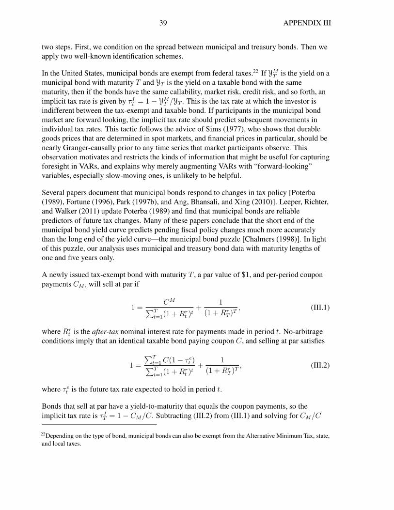
39 APPENDIX III

two steps. First, we condition on the spread between municipal and treasury bonds. Then we

apply two well-known identification schemes.

In the United States, municipal bonds are exempt from federal taxes.22 If YMT is the yield on a

municipal bond with maturity T and YT is the yield on a taxable bond with the same

maturity, then if the bonds have the same callability, market risk, credit risk, and so forth, an

implicit tax rate is given by τ IT = 1− YMT /YT . This is the tax rate at which the investor is

indifferent between the tax-exempt and taxable bond. If participants in the municipal bond

market are forward looking, the implicit tax rate should predict subsequent movements in

individual tax rates. This tactic follows the advice of Sims (1977), who shows that durable

goods prices that are determined in spot markets, and financial prices in particular, should be

nearly Granger-causally prior to any time series that market participants observe. This

observation motivates and restricts the kinds of information that might be useful for capturing

foresight in VARs, and explains why merely augmenting VARs with “forward-looking”

variables, especially slow-moving ones, is unlikely to be helpful.

Several papers document that municipal bonds respond to changes in tax policy [Poterba

(1989), Fortune (1996), Park (1997b), and Ang, Bhansali, and Xing (2010)]. Leeper, Richter,

and Walker (2011) update Poterba (1989) and find that municipal bonds are reliable

predictors of future tax changes. Many of these papers conclude that the short end of the

municipal bond yield curve predicts pending fiscal policy changes much more accurately

than the long end of the yield curve—the municipal bond puzzle [Chalmers (1998)]. In light

of this puzzle, our analysis uses municipal and treasury bond data with maturity lengths of

one and five years only.

A newly issued tax-exempt bond with maturity T , a par value of $1, and per-period coupon

payments CM , will sell at par if

1 =CM

∑Tt=1(1 +Rτ

t )t+

1

(1 +RτT )T

, (III.1)

where Rτt is the after-tax nominal interest rate for payments made in period t. No-arbitrage

conditions imply that an identical taxable bond paying coupon C , and selling at par satisfies

1 =

∑Tt=1C(1− τ et )

∑Tt=1(1 +Rτ

t )t

+1

(1 +RτT )T

, (III.2)

where τ et is the future tax rate expected to hold in period t.

Bonds that sell at par have a yield-to-maturity that equals the coupon payments, so the

implicit tax rate is τ IT = 1− CM/C . Subtracting (III.2) from (III.1) and solving for CM/C

22Depending on the type of bond, municipal bonds can also be exempt from the Alternative Minimum Tax, state,

and local taxes.

40 APPENDIX III

gives

τ IT =T∑

t=1

ωtτet , (III.3)

where ωt = δt/∑T

t=1 δt and δt = (1 +Rτt )

−t. The current implicit tax rate is a weighted

average of discounted expected future tax rates from t = 1 to T and should respond

immediately to news about anticipated future tax changes.

Equation (III.3) makes plain the advantages of using municipal bond spreads to capture

information flows about pending tax changes. First, there is no need to specify a priori the

period of foresight. Assuming market efficiency, the implicit tax rate reveals the extent to

which agents do or do not have foresight. Second, there is no need to specify a functional

form for information flows. In the previous section, we modeled information flows as coming

from one of several possible information processes. We would have to conduct a similar

sensitivity analysis if we were estimating a DSGE model. Using the implicit tax rate avoids

taking an a priori stand on the nature of information flows.

We turn to two prominent identification strategies that have acknowledged foresight in the

fiscal VAR literature—Blanchard and Perotti (2002) (BP) and Mountford and Uhlig (2009)

(MU). We derive conditions under which these identification schemes capture the true

information flows. We then augment each identification strategy by conditioning on implicit

tax rates and argue that this additional step alleviates the problems associated with foresight.

1. Blanchard and Perotti (2002)

BP estimate a quarterly VAR in output, y, government revenues net of transfers (including

interest payments), τ , and government spending (government consumption plus government

investment), g. The data are logarithms of real, per capita variables. We allow for both a

deterministic trend (quadratic in logs) and a stochastic trend (unit root with drift), as BP do.

Tests overwhelmingly support the causal priority of the implicit tax rate series in BP’s VAR

system. A test of whether lags of other variables help to predict spreads, given past

information on spreads, yields χ2 statistics with significance levels of 0.23 (deterministic

detrending) and 0.34 (stochastic detrending).23

23Forni and Gambetti (2010) and its references contain detailed discussion of tests for “informationalsufficiency” of a VAR. According to their criteria, our test satisfies a necessary but not sufficient condition for

fundamentalness. Sufficiency requires testing the null of no Granger causality against the principal components

from a factor model that contains a large set of macroeconomic data. For reasons discussed in the conclusion we

avoid using a factor model framework.

41 APPENDIX III

Write the reduced-form residuals from this VAR as

uτt =aτyuyt + bτge

∗gt + e∗τt

ugt =agyuyt + bgτe

∗τt + e∗gt

uyt =cyτuτt + cygu

gt + e∗yt

(III.4)

If agents have sufficient foresight, as BP themselves note and section 3 above documents, the

BP VAR will be misspecified and will result in biased inference. To account for such bias, we

let e∗gt , e∗τt , and e∗yt denote the shocks associated with the VAR representation. We

differentiate these shocks from the structural shocks available to the agents of the economy

(which we denote egt , eτt , and eyt ).

24

Section VIII of BP derives a mapping from the e∗t shocks to the shocks observed by the

agents, et, that follows from augmenting the VAR as

τt = a1yt + A11(L)τt−1 + A12(L)yt−1 + e∗τt (III.5)

yt = c0Et(τt+1) + c1τt + A21(L)τt−1 + A22(L)yt−1 + e∗yt (III.6)

where now output at date t responds to expected taxes at t+ 1. When agents have foresight, it

is likely that output will depend not only on current and lagged taxes but also on expected

taxes. BP show how the innovation in (III.5) led one quarter, e∗τt+1, can be used to instrument

for the expectational effects in (III.6). For this instrumental variables approach to be valid,

two stringent assumptions must hold. First, agents must have exactly one quarter of

foresight—no more, no less. Second, the innovation, e∗τt , in (III.5) cannot be correlated with

other shocks in the VAR.

Neither assumption is likely to hold in practice. As the previous section argues, the length of

foresight is likely to be much longer than one quarter and it varies substantially over time.

The BP identification scheme cannot handle more than one quarter of foresight because that

would require an implausible lag in the discretionary response of fiscal policy. With one

quarter of foresight, the BP identification requires no discretionary response of fiscal policy

to output realizations both this quarter and last quarter. Amending (III.6) with Etτt+2, which

allows for two quarters of foresight, requires that there is no discretionary response of fiscal

policy to output for three quarters, and so on. If agents have more than one quarter of

foresight, it is also very likely that the innovation e∗τt in (III.5) will be correlated with other

shocks in the VAR. The innovation from the VAR in that example is a convolution of the tax

and technology shocks. This suggests that the instrument used by BP to account for foresight

will be only weakly correlated with the explanatory variable.

24To confront the non-uniqueness described in section 4, BP identify the et shocks by arguing that legislative

lags ensure that there can be no within-quarter adjustment of fiscal policy to unexpected changes in GDP, other

than “automatic effects of activity on taxes and spending under existing fiscal policy rules.” Automatic effectsoperate through parameters aτy and agy , which are elasticities of tax revenues and government purchases with

respect to output. BP then show that once aτy and agy are calibrated to 2.08 and 0, respectively, uτt − aτyu

yt

and ugt − agyu

yt can be used as instruments in estimating cyτ and cyg. The final two parameters are set to either

bτg = 0 and bgτ 6= 0 or vice versa to triangularize the fiscal sector.

42 APPENDIX III

Now augment BP’s VAR system with data on the spread, s, between municipal bonds and

treasury bonds (the implicit tax rate)

uτt =aτyuyt + aτsu

st + bτge

gt + eτt

ugt =agyuyt + agsu

st + bgτe

τt + egt

uyt =cyτuτt + cygu

gt + eyt

ust =csτuτt + csgu

gt + csyu

yt + est

(III.7)

By conditioning on the implicit tax rate, the econometrician no longer needs to use the

innovation e∗τt as an instrument for the expectation in (III.6). An efficient municipal bond

market makes the implicit tax rate equivalent to the expectation in (III.6), as (III.3) makes

clear. This relaxes the stringent assumptions that BP’s identification of foresight requires;

conditioning on the municipal bond spread posits that the innovations in (III.7) are the true

structural shocks (i.e., that the observables augmented with the implicit tax rate spans the

space of the shocks observed by the agents), and all that is left to achieve identification is a

rotation of the covariance matrix. We make the reasonable assumption that news contained in

interest-rate spreads has no direct impact on current output, tax revenues, and spending. This

assumption sets both aτs and ags to zero and implies that the relationship between the

reduced-form and structural innovations for the tax and spending shocks of (III.7) are

identical to those of (III.4). We can now apply BP’s identification of these shocks. We also

identify the “news” shock, est , (again following the lead of BP) by using the reduced-form

shocks and parameters as instruments to estimate csτ , csg, and csy.25 To facilitate comparison,

we use the same data and follow the same detrending procedures as BP. We refer the reader

to Section III of BP for a more detailed discussion of the data and empirical approach.

Figure 2 plots the estimated mean responses to an unanticipated tax revenue shock (panels C

and D) and to a shock to the implicit tax rate (panels A and B), with one-standard deviation

bands computed by Monte Carlo simulations based on 500 replications. Solid lines represent

the deterministic-trend model and dashed lines the stochastic-trend VAR. Following BP, we

transform the original impulse responses to report the dollar response of each variable to a

dollar shock in the fiscal variables. We use the tax revenue data to transform the implicit tax

rate so that the impulse response is interpreted as a dollar shock to anticipated tax revenue.

Panels B and D of the figure condition on a five-year implicit tax rate, implying that agents

have a maximum of five years of foresight, but results are robust to implicit tax rates with

maturity less than five years.

Panel C is identical to BP’s figure III and shows that the response of output to a surprise tax

increase is negative and significant. The heavy solid line in panel C is BP’s

instrumental-variable estimate of the effect of foresight (figure VI in BP). That solid line

represents the “upper bound” on the anticipatory effects of foresight, according to BP. As the

figure shows, identifying foresight using their approach generates a positive response on

impact, in contrast to the negative response from the VAR that ignores foresight altogether.

25More specifically, uτt − atyu

yt , u

gt − agyu

yt , and u

yt − cyτu

τt − cygu

gt are used as instruments for csτ , csg and

csy , respectively.

43 APPENDIX III

4 8 12 16 20

−0.2

−0.1

0

0.1

0.2

0.3

4 8 12 16 20−0.5

0

0.5

1

1.5

4 8 12 16 20−2

−1.5

−1

−0.5

0

0.5

4 8 12 16 20−4

−2

0

2

4

Deterministic

Stochastic

BP estimated effects of foresight

Panel C: Output to Tax Revenue Shock

BP Figure III and anticipated effects

Panel D: Implicit Tax to Tax Revenue Shock

Panel A: Output to Implicit Tax Shock Panel B: Revenues to Implicit Tax Shock

Figure 2. Estimated mean responses for deterministic trend (solid lines) and stochastic trend

(dashed lines) to a positive tax revenue shock (panels C, D) and positive implicit tax rate shock

(panels A, B) with one-standard-deviation bands.

44 APPENDIX III

Beyond the impact period, BP’s methodology does not, however, deliver responses that are

statistically different from the VAR that ignores foresight. This result leads BP to conclude,

“there is not much evidence of an effect of anticipated tax changes on output [p. 1353].”

Panel A contrasts sharply with BP’s findings: output rises substantially and significantly after

an increase in the implicit tax rate. The anticipatory effects of fiscal foresight last well beyond

the initial quarter and, in the short run, anticipated increases in tax rates are expansionary.

Our approach generates markedly different results from BP primarily because the implicit tax

rate provides flexible information about the degree of foresight. BP’s identification permits

only one quarter of foresight, while ours allows a maximum of five years. This is an example

of the kind of a priori restriction on information flows that can drive inferences about

foresight. Panels B and D of the figure corroborate the plausibility of our identification by

showing that tax revenues respond positively and significantly to a positive innovation in the

implicit tax rate, as theory suggests. Further corroboration of the identification comes from

the fact that the implicit tax rate does not respond significantly to innovations in taxes, which

theory also predicts (panel D).

0 qtr 4 qtrs 8 qtrs 12 qtrs 20 qtrs

Panel A: Blanchard-Perotti, Deterministic Trend

GDP (BP) −0.69∗ −0.74∗ −0.72∗ −0.42∗ −0.22GDP (U) −0.84∗ −1.15∗ −0.95∗ −0.36 −0.06GDP (A) 0.03 0.19∗ 0.13∗ −0.02 −0.10∗

Panel B: Blanchard-Perotti, Stochastic Trend

GDP (BP) −0.70∗ −1.07∗ −1.32∗ −1.30∗ −1.29∗

GDP (U) −0.71∗ −1.15∗ −1.39∗ −1.34∗ −1.33∗

GDP (A) 0.04 0.17∗ 0.18∗ 0.18∗ 0.17∗

Panel C: Mountford-Uhlig, Output Multipliers

GDP (MU) −0.29∗ −0.79∗ −1.23∗ −1.61∗ −0.60GDP (U) −0.27 −1.04∗ −1.64∗ −1.81∗ −1.05GDP (A) −0.10∗ 0.04∗ 0.09 0.02 0.03

Panel D: Mountford-Uhlig, Investment Multipliers

INV (MU) −0.19 −0.27∗ −0.38 −0.46 −0.14INV (U) −0.23 −0.31∗ −0.50∗ −0.42 −0.27INV (A) 0.03 0.12∗ 0.14∗ 0.10 0.09

Table 4. Output and Investment Multipliers for an Implicit Tax Shock (A) and Tax Revenue

Shock (U). An asterisk indicates zero is outside of the region between the two one-standard

deviation bands. BP denotes the numbers from the VAR without municipal bonds.

Panels A and B of table 4 report estimated output multipliers for the estimated VAR. The

table also records results from BP’s table III for comparison. The primary difference between

the BP multipliers and ours is that we allow for the anticipatory effect that arises from

foresight—the inside and outside lags. The row labeled GDP (A) is the multiplier associated

with an innovation in the implicit tax rate arising from an anticipated increase in tax rates.

45 APPENDIX III

The row labeled GDP (U) is the multiplier associated with an innovation in the tax revenue

shock, identified as the effect of an unanticipated tax cut.

Several features stand out. First, for the majority of the horizon and both detrending methods,

the output multiplier for the implicit tax rate is positive, so higher anticipated taxes raise

output in the short run. With the lone exception of the 1- and 12-quarter multipliers, all

multipliers in the anticipatory horizon have one-standard deviation error bands that do not

cross zero. The peak positive responses are 0.19 at 4 quarters (deterministic trend model) and

0.18 (stochastic trend model). Second, the multipliers associated with the implicit tax rate are

much smaller in absolute value than those from the tax revenue shock. This suggests that

agents probably do not have perfect foresight, on average. Perfect foresight would imply

movements in macro aggregates that are about the same magnitude as for unanticipated

shocks (assuming identical variances). The relatively muted response of output to a shock in

the implicit tax rate suggests that more intricate information flows than perfect foresight (e.g.,

moving-average processes for news) are probably at work. Implicit tax rates capture this kind

of subtlety. Finally, unanticipated tax hikes have substantially larger effects in the VAR that

includes the implicit tax rate than in the BP specification, particularly for the deterministic

trend. For example, the one-standard deviation error bands on the 4-quarter multiplier are

−1.64 and −0.65, which nearly exclude the BP estimate of−0.74. This is consistent with the

numerical evidence presented in section 3, where the econometrician consistently

underestimates the multiplier.

Our finding that news of higher taxes increases economic activity over much of the

anticipation period, as figure 2 depicts, echoes results from two very different methodologies.

In a case study, House and Shapiro (2006) argue that the phased-in tax reductions enacted by

the 2001 Economic Growth and Tax Relief Reconciliation Act played a significant role in

creating the unusually slow recovery from the 2001 recession. By feeding the legislated paths

of marginal tax rates on labor and capital into an RBC model, the authors generate a path of

equilibrium GDP that shares qualitative features with panel A of figure 2.

Mertens and Ravn (2011) augment a VAR with Romer and Romer’s (2010) anticipated tax

liabilities series, which they treat as strictly exogenous in the VAR. Mertens and Ravn append

to each equation of the VAR a distributed lag of q periods in future tax liabilities. They

estimate that an anticipated tax increase induces a boom in output whose amplitude and

duration increase with the period of foresight q. In contrast to our approach with

muni-treasury spreads, Mertens and Ravn must specify a priori the period of foresight and

maintain that anticipated taxes are exogenous—assumptions that are critical to the

quantitative effects they obtain. Nonetheless, the qualitative effects closely resemble those in

panel A of our figure.

Despite their different methodologies, House-Shapiro and Mertens-Ravn share a common

economic explanation for their findings, which also applies to the RBC model in section 3.

Anticipated tax changes generate wealth effects that kick in immediately—upon arrival of the

news—but the substitution effects, which operate on critical economic margins, do not affect

behavior until the tax rates have changed. In a conventional model, expected tax increases

46 APPENDIX III

reduce wealth, which induces agents to work harder, increasing employment and output

immediately.

Anticipated tax changes have sharply different macroeconomic impacts in our model, which

includes a direct measure of tax news and a flexible specification of foresight, than in the

instrumental variables, tightly circumscribed approach that BP take. These differences

underscore the importance of modeling information flows.

2. Mountford and Uhlig (2009)

Mountford and Uhlig (2009) impose restrictions directly on the shape of the impulse

responses of the VAR to identify economic shocks, following the work of Faust (1998),

Canova and Pina (2000), Uhlig (2005), and Canova and Pappa (2007). Like BP, MU identify

two fiscal policy shocks—a government spending shock and a government revenue shock.

They define a fiscal shock as a positive reaction of the respective fiscal variable for four

consecutive periods, including the impact response. This is to ensure that only substantial

movements in fiscal variables are counted as “shocks.” Fiscal shocks are required to be

orthogonal to business cycle shocks and monetary policy shocks. Business cycle shocks are

defined as a shock which jointly moves output, consumption, nonresidential investment and

government revenue in the same direction for four quarters following the shock.26 A

monetary policy shock is defined as a shock that moves interest rates up and reserves and

prices down for four quarters after the shock.

Like with most identification schemes, this one intends to identify rotations of the covariance

matrix. Caldara and Kamps (2010) and Caldara (2011) show that the sign restriction

approach of MU can be reinterpreted as pinning down the elasticities associated with the BP

system (III.4). And like BP, MU acknowledge the importance of foresight and impose

additional restrictions to account for it. MU argue that anticipated fiscal policy changes can

be identified by imposing zero restrictions on the responses of fiscal variables over the period

of fiscal foresight, reflecting the idea that the isolated policy shock is news about a change in

future, but not current, policy variables.

Under what conditions will the MU identification scheme deliver correct inference? As the

analytical section shows, fiscal foresight does not imply a zero response of all fiscal variables

over the foresight period. The various fiscal rules considered in the previous section suggest

that this is an exceptional situation. In the special case where the tax rate is exogenous and

follows the simple rule

τt = euτ,t + ετ,t−q (III.8)

26To select among the many rotations consistent with this definition of the business cycle shock, MU impose the

criterion that substantial movements in output, consumption, nonresidential investment and government revenue

must be attributed to business cycle shocks.

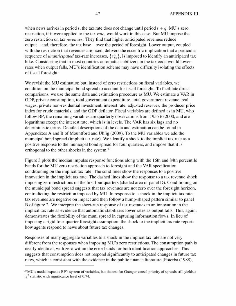
47 APPENDIX III

when news arrives in period t, the tax rate does not change until period t+ q. MU’s zero

restriction, if it were applied to the tax rate, would work in this case. But MU impose the

zero restriction on tax revenues. They find that higher anticipated revenues reduce

output—and, therefore, the tax base—over the period of foresight. Lower output, coupled

with the restriction that revenues are fixed, delivers the eccentric implication that a particular

sequence of unanticipated tax-rate increases, euτ,t, is imposed to identify an anticipated tax

hike. Considering that in most countries automatic stabilizers in the tax code would lower

rates when output falls, MU’s identification scheme may have difficulty isolating the effects

of fiscal foresight.

We revisit the MU estimation but, instead of zero restrictions on fiscal variables, we

condition on the municipal bond spread to account for fiscal foresight. To facilitate direct

comparisons, we use the same data and estimation procedure as MU. We estimate a VAR in

GDP, private consumption, total government expenditure, total government revenue, real

wages, private non-residential investment, interest rate, adjusted reserves, the producer price

index for crude materials, and the GDP deflator. Fiscal variables are defined as in MU, who

follow BP; the remaining variables are quarterly observations from 1955 to 2000, and are

logarithms except the interest rate, which is in levels. The VAR has six lags and no

deterministic terms. Detailed descriptions of the data and estimation can be found in

Appendixes A and B of Mountford and Uhlig (2009). To the MU variables we add the

municipal bond spread (implicit tax rate). We identify a shock to the implicit tax rate as a

positive response to the municipal bond spread for four quarters, and impose that it is

orthogonal to the other shocks in the system.27

Figure 3 plots the median impulse response functions along with the 16th and 84th percentile

bands for the MU zero restriction approach to foresight and the VAR specification

conditioning on the implicit tax rate. The solid lines show the responses to a positive

innovation in the implicit tax rate. The dashed lines show the response to a tax revenue shock

imposing zero restrictions on the first four quarters (shaded area of panel D). Conditioning on

the municipal bond spread suggests that tax revenues are not zero over the foresight horizon,

contradicting the restriction imposed by MU. In response to a shock in the implicit tax rate,

tax revenues are negative on impact and then follow a hump-shaped pattern similar to panel

B of figure 2. We interpret the short-run response of tax revenues to an innovation in the

implicit tax rate as evidence that automatic stabilizers lower rates as output falls. This, again,

demonstrates the flexibility of the muni spread in capturing information flows. In lieu of

imposing a rigid four-quarter foresight assumption, the shock to the implicit tax rate reports

how agents respond to news about future tax changes.

Responses of many aggregate variables to a shock in the implicit tax rate are not very

different from the responses when imposing MU’s zero restrictions. The consumption path is

nearly identical, with zero within the error bands for both identification approaches. This

suggests that consumption does not respond significantly to anticipated changes in future tax

rates, which is consistent with the evidence in the public finance literature [Poterba (1988),

27MU’s model expands BP’s system of variables, but the test for Granger-causal priority of spreads still yields a

χ2 statistic with significance level of 0.74.

48 APPENDIX III

0 5 10 15 20

−0.6

−0.4

−0.2

0

0.2

0.4

0.6

0.8

0 5 10 15 20

−0.6

−0.4

−0.2

0

0.2

0.4

0.6

0.8

0 5 10 15 20

−2

−1

0

1

2

3

0 5 10 15 20

−1

0

1

2

3

Panel A: Output Panel B: Consumption

Panel C: Non-residential Investment Panel D: Tax Revenues

Figure 3. Estimated median responses with 16th and 84th percentile bands for MU VAR

specification to a positive tax revenue shock (dashed lines) and MU VAR with muni spread to

a positive implicit tax rate shock (solid lines).

49 APPENDIX IV

Parker (1999), Souleles (1999, 2002)]. However, unlike the conclusions reached in those

papers, we do not take this as evidence of the lack of foresight. Many of the aggregate

variables respond in significant ways to the news in implicit tax rates. For example, the path

of non-residential fixed investment mimics the hump-shaped response of tax revenues. An

anticipated increase in tax rates produces a positive and significant response of investment for

several quarters, which contrasts to the negative or zero response generated by imposing

MU’s zero restrictions.

Effects of anticipated taxes in figure 3 are consistent with economic theory. Mertens and

Ravn (2011) emphasize the distinction between consumption of durables and nondurables in

understanding the impacts of anticipated tax changes. In their empirical and theoretical

analyses, Mertens and Ravn find that, while foresight can have a significant effect on durable

consumption, nondurables are less likely to move in response to anticipated changes in tax

rates.28 Auerbach (1989) emphasizes the role of investment adjustment costs when

examining the dynamic effects of anticipated taxes on investment. That investment responds

positively and significantly over many quarters suggests that investment adjustment costs

may be low: if adjustment costs were high, firms would begin to decrease investment

immediately in response to an anticipated tax increase. Finally, counter to the results found in

the BP specification, panel A shows that output responds negatively to an anticipated tax

increase in both identification schemes. One explanation for the differences across BP and

MU can be attributed to the particular rotation of the covariance matrix implemented by MU.

Caldara and Kamps (2008) map the elasticities estimated by BP in (III.4) into the implied

elasticities from imposing the MU sign restrictions. They find that MU impose a much higher

within-quarter elasticity of net taxes with respect to output. The higher elasticity will drive

down the response of output to an implicit tax rate shock.

Panels C and D of table 4 report estimates of the output and investment impact multipliers to

an innovation in the tax revenue shock (U), the implicit tax rate (A) and the tax revenue

shock in the original MU specification. As was the case with the BP identification, the

estimated effects of an anticipated tax decline are smaller than the effects of unanticipated

shocks. Also similar, the MU identification underestimates the size of the multipliers. For

example, at the eight-quarter horizon, the MU estimate of the median output multiplier falls

around the 20th percentile of the posterior for the tax revenue shock estimated from the

expanded VAR. Table 4 makes clear that accounting for foresight changes the estimated

output and investment multipliers associated with tax shocks.

APPENDIX IV. ASSESSING THE EX-ANTE APPROACH

We share the view of the ex-ante approach that, in the presence of fiscal foresight,

conventional fiscal VARs misalign the information sets of economic agents and the

econometrician. In the context of the model in section 2, conventional VARs estimate

28They reconcile this empirical finding with theory by assuming habit formation in consumption andcomplementarity in consumption goods, which smooth out the wealth effects during the period of foresight.

50 APPENDIX IV

systems in current and past values of capital (or output) and revenues. Fiscal foresight implies

that those systems are not invertible and do not adequately capture the fiscal news to which

agents respond. When tax rates are exogenous, as in the simple example, information sets are

correctly aligned by including future tax rates in the VAR. This results in a VAR system in

kt, τt+q and now the fundamental representation is invertible. The ex-ante approach

essentially applies this principle by seeking instruments for expected future tax obligations.

The discussion in section 2 make this interpretation more precise. Although non-invertibility

of the moving average representation implies there is no autoregressive representation in

which the true fiscal news is a function of current and past endogenous variables, there is an

autoregressive representation in the fiscal news and future endogenous variables. The ex-ante

approach uses forecasts of revenue changes associated with tax legislation to instrument for

the information agents possess about future taxes. To infer the effects of anticipated taxes on

output, the ex-ante approach regresses output against forecasted revenue changes, among

other variables, and interprets the estimated coefficients causally. To assess the ex-ante

approach, we examine the quality of instruments employed.

Of course, tax rates are not exogenous. They are the outgrowth of a complex set of economic

and political decisions. Recognizing the intrinsic endogeneity of tax policy decisions, Romer

and Romer (2010, 2007) use a narrative method to compile data series that decompose the

forecasted revenue consequences of federal tax changes into “endogenous” and “exogenous”

components. Mertens and Ravn (2010) use the Romers’ compiled data series. They

generalize the Romers’ empirical work and lay out an intricate DSGE model to interpret their

estimates of the impacts of anticipated and unanticipated changes in taxes. Whereas the

Romers find only weak evidence that private agents react to anticipated tax changes, Mertens

and Ravn obtain provocative and striking results reminiscient of Branson, Fraga, and

Johnson’s (1986) argument about the Reagan tax cuts: anticipated tax cuts induce sharp

economic slowdowns during the period of fiscal foresight, and may even produce recessions.

In this section we use a standard real business cycle model with proportional capital and

labor tax rates to simulate equilibrium data, including forecasted revenue changes induced by

anticipated and unanticipated tax disturbances. We then run regressions using simulated data

and compare the estimated effects of foreseen changes in tax rates to the true effects of fiscal

foresight. Because the simulated data and revenue forecasts are generated by a single

coherent model, if the ex-ante approach is efficacious, the regressions should recover the true

effects almost exactly.

Before we can proceed with this test of the ex-ante method, we first must embed the narrative

identification scheme in a formal theoretical model.

A. Formalizing the Narrative Identification

The Romers distinguish between “endogenous” changes in taxes—ones induced by short-run

countercyclical concerns and those undertaken because government spending was

changing—and “exogenous” changes in taxes—those that are responses to the state of

51 APPENDIX IV

government debt or to concerns about long-run economic growth. To avoid confusion with

other definitions, we shall refer to these as “RR endogenous” and “RR exogenous”

components of tax policy behavior.

We specify a tax rule that includes the various motivations for tax changes that the Romers

consider and embeds both anticipated and unanticipated shocks to taxes. Alternative

parametric specifications of policy coincide with different formalizations of the narrative

identification scheme. Our message is that the performance of the ex-ante approach hinges

critically on the precise formalization attributed to the narrative identification.

To reflect the distinction the Romers draw between “endogenous” countercyclical concerns

and “exogenous” long-run concerns, it is convenient to decompose output into business

cycle, yCt , and trend, yTt , components. A rule for tax rates that embeds this multiplicity of

motivations for tax changes is given by

τt = ρ(L)τt−1 +P∑

j=−P

µCj EtyCt+j +

M∑

j=−M

βjEtgt+j

︸ ︷︷ ︸

“RR endogenous”

+P∑

j=−P

µTj EtyTt+j +

N∑

j=−N

γjEtsBt+j−1 + ετ,t−q + euτ,t

︸ ︷︷ ︸

“RR exogenous”

(IV.1)

The fiscal authority’s choice of the current tax rate is permitted to respond systematically to

current, past, and expected fluctuations in output at both business cycle and trend frequencies

and to current, past, and expected changes in government spending (gt+j) and government

indebtedness as measured by the debt-to-output ratio (sBt+j−1). The rule also embeds an

unanticipated shock, euτ,t, and “news” about the tax rate that arrived q periods in the past,

ετ,t−q. Both of these shocks are assumed to be unrelated to economic conditions.29

To study the Romers’ identification, we simplify (IV.1) by restricting the “RR endogenous”

component and the feedback from trend output movements in the “RR exogenous”

component. We also specialize the timing of the response to the state of government debt to

coincide with the period of foresight, q, and allow only one lag of the tax rate to enter,

ρ(L) = ρ. This simplifies (IV.1), written in terms of its anticipated and unanticipated parts, to

τt = ρτt−1 + µCyt + ξt−q + euτ,t (IV.2)

where

ξt−q = µT yt−q−1 + γsBt−q−1 + ετ,t−q (IV.3)

is the fiscal foresight, which stems from both systematic responses of taxes to past economic

and fiscal conditions and exogenous news about tax legislation. By simplifying the tax rule to

29Although in their papers the Romers do not explicitly interpret tax legislation as containing shock components,

in private communication David Romer confirmed that this interpretation is not inconsistent with their views.

52 APPENDIX IV

restrict the sources of feedback from the economy to expected future tax rates, we are likely

to bias our results in favor of the ex-ante narrative approach.

It might seem like a stretch to model the response of tax policy to concerns about long-run

economic growth as we do in the definition of ξt−q . But several large tax bills that Romer and

Romer (2007) label as long-run, “exogenous” tax changes could easily be categorized as

“endogenous” responses to short-term economic conditions. Stein (1996) documents that

President Kennedy was prompted to change his position on a tax cut by the stalled recovery

in 1962 and 1963 from the 1960-1961 recession.30 The Economic Recovery Act of 1981

signed by President Reagan is widely regarded as driven by philosophical considerations.

But the supply-side promise to stimulate growth without triggering inflation, is arguably an

endogenous reaction to the stagflation of the 1970s and early 1980s. The Romers classify two

recent tax cut bills signed by President Bush—part of the Economic Growth and Tax Relief

Reconciliation Act of 2001 and the Working Families Tax Relief Act of 2003—as long-run

“exogenous” events. The Economic Report of the President (2002, p. 44) argues, “The

President laid a strong foundation for growth in 2001 with the Economic Growth and Tax

Relief Reconciliation Act. This package provides a powerful stimulus for future growth....”

But the tax cut bills enacted in 2001, 2002, and 2003 were also clearly linked to the recession

in 2001 and its subsequent “jobless” recovery. Congressional Quarterly Press (2006)

documents that in the case of the 2003 tax cut, President “Bush continued to insist that tax

cuts were the best way to deal with both the budget deficit and the slow pace of job creation”

[p. 42]. Evidently there is no sharp distinction between tax cuts motivated by countercyclical

considerations and those driven by a desire to boost economic growth in the long run.

We have specified a rule for future tax rates, but the Romers and Mertens and Ravn employ

forecasts of tax revenues. We simulate the model to generate data and model-generated

forecasts of revenue changes due to both the unanticipated, euτ,t, and anticipated, ετ,t−q,exogenous disturbances to capital and labor tax rates. Although the Romers estimate

single-equation regressions, we reproduce the slightly more general estimated VARs that

Mertens and Ravn use to report the dynamic impacts of the two kinds of tax shock.

Specifically, we estimate

Xt = A + CXt−1 +24∑

i=0

DiTut−i +

24∑

i=0

FiTat−i +

6∑

i=1

GiTat+i + ut, (IV.4)

where Xt is a data vector that includes output, consumption, investment, and hours worked,

Xt = [lnyt, ln ct, ln it, ln lt]′

. T ut is revenue changes divided by output due to the

unanticipated tax shock and T at+i is the out-of-sample forecast of revenue changes for

anticipated tax policy divided by output.31 Forecasts are conditional on information at t, for

30The unemployment rate fell from 6.7 percent in October, 1961 to 5.5 percent in March, 1962 and then leveled

off for the remainder of 1962. Output growth was slower than in the previous year. Stein (1996) writes that theproposal to cut taxes “was a delayed response to a chronic condition after hopes of a spontaneous recovery were

dimmed” [p. 408].

31The Romers’ data set scales revenues by actual future output, which treats a function of future shock

realizations as a regressor in (IV.4). We follow their procedure in the simulations.

53 APPENDIX IV

each date in the simulated data. Since the DSGE model we use to generate data has separate

exogenous shocks for capital and labor tax rates, estimation of (IV.4) is done separately for

the two taxes; therefore, to estimate the effects of an anticipated capital tax cut, T ut and T at in

(IV.4) are associated with capital tax changes, and vice versa for labor taxes.32

Romer and Romer and Mertens and Ravn share the critical maintained assumption that

forecasted revenue changes are the exogenous news about taxes. This assumption explains

why the system in (IV.4) does not include an equation that describes the evolution of

revenues or government debt over time. Implicitly in Romer and Romer and explicitly in

Mertens and Ravn’s theoretical model, lump-sum transfers are assumed to adjust to keep the

government solvent. But this Ricardian assumption conflicts with the way that “RR

exogenous” changes in taxes are constructed: as the rule in (IV.1) makes clear, that

constructed measure includes legislative actions that are a response to budget deficits or the

state of government indebtedness.

B. Simulation Results

Revenue forecasts provide an important input to fiscal decisions by policy makers at both the

federal and the state levels. Large fluctuations in tax bases make revenues notoriously

difficult to forecast accurately. One way to mimic the difficulties inherent in forecasting

revenues is to add measurement error that is unrelated to economic fundamentals. An

alternative, more economically grounded method, is simply to build into the theory multiple

sources of uncertainty. In addition to unanticipated and anticipated shocks to capital and

labor tax rates, the DSGE model used to simulate data includes several other sources of

random variation—shocks to technology, preferences over leisure, government spending, and

government transfers. Multiple sources of uncertainty imply that forecasted tax rates, Etτt+q,are a function of many different structural disturbances whose effects on taxes operate

through the endogenous variables.

Figures 4-7 depict the paths of consumption and output in response to six-period foresight

about cuts in labor and capital tax rates. Shocks to tax rates are assumed to be correlated,

though not perfectly, as they are in data. Panels (a)-(d) reflect alternative parametric

formalizations of the narrative identification. These impulse response functions are derived

from estimates of (IV.4) using 1000 sample paths generated by the growth model. Heavy

solid lines are the true theoretical impacts; thin solid lines are the means of the estimated

impacts; dashed lines are 68 percent probability bands for the estimated responses.

Panel (a) is the best-case scenario for the narrative approach. It shuts down all responses of

tax rates to economic conditions and has lump-sum transfers adjust to stabilize debt. The

32The Romers and Mertens and Ravn do not distinguish between capital and labor tax changes in their empirical

work. Sorting revenue forecasts into those due to capital and labor tax policy changes is a difficult task, as a

single provision in a tax bill often affects both capital and labor income taxes simultaneously. For example, anacross-the-board individual income tax rate reduction would change both types of taxes. In addition, Yang

(2005) shows that anticipated capital and labor taxes can have very different effects and that assuming a single

tax rate on both sources of income can mask the impacts of fiscal foresight.

54 APPENDIX IV

0 5 10 15 20 25 30−0.5

00.5

11.5

(a)

0 5 10 15 20 25 30−0.4−0.2

00.20.4

(b)

0 5 10 15 20 25 30

−0.20

0.20.4

(c)

0 5 10 15 20 25 30

−0.2

0

0.2

0.4

(d)

Figure 4. Responses of Consumption to 6-Period Foresight of Labor Taxes.

Panel (a) µC = 0, µT = 0, γT = −.1, σK = .025, σL = .02Panel (b) µC = 1, µT = 0, γτ = .05, σK = .025, σL = .02Panel (c) µC = 1, µT = .5, γτ = .05, σK = .025, σL = .02

Panel (d) µC = 1, µT = .5, γτ = .05, σKa = .0375, σKu = .0125, σLa = .03, σLu = .01

policy rule becomes τt = ρτt−1 + ετ,t−q + euτ,t; transfers evolve according to Tt = γTsBt−1,

with γT > 0. Across all four figures, estimates of (IV.4) do a very good job of recovering the

theoretically correct responses.33

Once tax rates respond to debt, estimates based on the VAR in (IV.4) can go badly astray over

both the period of foresight and longer horizons. Panels (b)-(d) each impose that labor and

capital tax rates adjust to stabilize debt (γτ > 0); they differ in the degree to which tax policy

choices react to output and in the relative variability of anticipated and unanticipated

exogenous disturbances to taxes. Panel (b) comes from a model that allows for automatic

stabilizers in the tax code (µC > 0); panel (c) includes both automatic stabilizers and fiscal

foresight that includes a systematic response to past output (µT > 0); panel (d) includes both

of these components but raises the variance of anticipated tax shocks relative to unanticipated

tax shocks, reflecting the fact that because most tax changes are implemented with a lag,

anticipated changes are more prevalent and more important. Modeling “RR exogenous” tax

33Discrepancies between the thin and the thick solid lines arise from the fact that the Romers and Mertens and

Ravn scale forecasted revenue changes by actual future GDP, a procedure that we mimic, whereas the true

theoretical responses do not include this scaling.

55 APPENDIX IV

0 5 10 15 20 25 30

−0.50

0.51

1.5

(a)

0 5 10 15 20 25 30−0.4−0.2

00.20.4

(b)

0 5 10 15 20 25 30−0.4−0.2

00.20.4

(c)

0 5 10 15 20 25 30

−0.2

0

0.2

(d)

Figure 5. Responses of Consumption to 6-Period Foresight of Capital Taxes.

Panel (a) µC = 0, µT = 0, γT = −.1, σK = .025, σL = .02Panel (b) µC = 1, µT = 0, γτ = .05, σK = .025, σL = .02Panel (c) µC = 1, µT = .5, γτ = .05, σK = .025, σL = .02

Panel (d) µC = 1, µT = .5, γτ = .05, σKa = .0375, σKu = .0125, σLa = .03, σLu = .01

changes as including a systematic response of tax rates—as opposed to lump-sum

transfers—to the state of government debt is fully consistent with the Romer’s narrative, so

panels (b)-(d) of the figures provide more appropriate assessments of the ex-ante approach.

The ex-ante approach may perform quite well over the period of foresight, as it does in

estimating the response of consumption to foresight about a capital tax rate cut in figure 5

(see also figure 6). But it can also perform very poorly. Figure 4 shows that an anticipated cut

in labor taxes creates a boom in consumption in the foresight period, while estimates of

(IV.4) find that a substantial recession is quite likely. A less pronounced slump in

consumption is estimated for the response of output to a foreseen capital tax cut, when the

correct theoretical response is a mild expansion [figure 7]. The inference that a recession

occurs before an anticipated cut in taxes coincides closely with Merten and Ravn’s results

from estimating (IV.4) based on the Romer’s data on changes in tax liabilities.

Difficulties with the ex-ante approach are not limited to inferences about the effects of

foresight over the short run. Figure 4 shows that over horizons of five or more years, it is very

unlikely that estimates of (IV.4), which die out rather quickly, will recover the medium-run

56 APPENDIX IV

0 5 10 15 20 25 30−1

0123

(a)

0 5 10 15 20 25 30

0

1

2

(b)

0 5 10 15 20 25 30−1

0

1

2

(c)

0 5 10 15 20 25 30−0.5

00.5

11.5

(d)

Figure 6. Responses of Output to 6-Period Foresight of Labor Taxes.

Panel (a) µC = 0, µT = 0, γT = −.1, σK = .025, σL = .02Panel (b) µC = 1, µT = 0, γτ = .05, σK = .025, σL = .02Panel (c) µC = 1, µT = .5, γτ = .05, σK = .025, σL = .02

Panel (d) µC = 1, µT = .5, γτ = .05, σKa = .0375, σKu = .0125, σLa = .03, σLu = .01

decline in consumption following a reduction in labor tax rates. The source of the

mispredictions is that the VAR system in (IV.4) treats the changes in revenues forecasts, the

T at+i terms, as exogenous “shocks” that are not systematically related to the state of the

economy. This treatment fails to provide agents with the structural information that

debt-financed tax cuts will ultimately bring forth higher tax rates still farther in the future. In

other words, given how the revenue forecasts are constructed, treating them as evolving

autonomously amounts to misspecifying the tax rule. Panels (b)-(d) of figure 4 make clear

that misspecification of the tax rule is the source of the medium-run mispredictions: when

lump-sum transfers adjust to stabilize debt, as in panel (a), the estimated system in (IV.4)

nails the responses at longer horizons.

Our simulation exercise dramatically understates the uncertainty inherent in revenue

forecasts because our model forecaster knows the true structure of the economy. If the

ex-ante approach cannot consistently work in our idealized laboratory, the noise associated

with actual revenue forecasts is likely to hinder severely the method’s ability to recover

anticipated tax effects.

57 APPENDIX IV

0 5 10 15 20 25 30−1

0

1

2

(a)

0 5 10 15 20 25 30−0.5

0

0.5

1

(b)

0 5 10 15 20 25 30−0.5

0

0.5

1

(c)

0 5 10 15 20 25 30

0

0.5

1

(d)

Figure 7. Responses of Output to 6-Period Foresight of Capital Taxes.

Panel (a) µC = 0, µT = 0, γT = −.1, σK = .025, σL = .02Panel (b) µC = 1, µT = 0, γτ = .05, σK = .025, σL = .02Panel (c) µC = 1, µT = .5, γτ = .05, σK = .025, σL = .02

Panel (d) µC = 1, µT = .5, γτ = .05, σKa = .0375, σKu = .0125, σLa = .03, σLu = .01

This assessment of the ex-ante approach employs a barebones real business cycle model and

a relatively crude specification of tax policy behavior. A model with many more parameters

and internal propagation mechanisms or a more sophisticated characterization of policy can

generate far more exotic dynamics. But greater complexity does not alter the basic message:

success of the ex-ante approach hinges on how the narrative method of identifying tax news

is formalized. Even simple theory can produce a wide range of conclusions about the efficacy

of the approach. Two factors emerge as critical to the success of the ex-ante approach: the

degree to which forecasted revenue changes reflect exogenous changes in taxes and the

relative volatility of the random components of tax decisions.

58 References

REFERENCES

ABEL, A. B. (1982): “Dynamic Effects of Permanent and Temporary Tax Policies in a q

Model of Investment,” Journal of Monetary Economics, 9(3), 353–373.

AN, S., AND F. SCHORFHEIDE (2007): “Bayesian Analysis of DSGE Models,”

Econometric Reviews, 26(2), 113–172.

ANG, A., V. BHANSALI, AND Y. XING (2010): “Taxes on Tax-Exempt Bonds,” The

Journal of Finance, 65(2), 565–601.

AUERBACH, A. J. (1989): “Tax Reform and Adjustment Costs: The Impact on

Investment and Market Value,” International Economic Review, 30(4), 939–962.

BARSKY, R., AND E. SIMS (2011): “News Shocks and Business Cycles,” Journal of

Monetary Economics, 58(3), 273–289.

BASU, S., AND J. G. FERNALD (1995): “Are Apparent Productive Spillovers a Figment

of Specification Error?,” Journal of Monetary Economics, 36(1), 165–188.

BEAUDRY, P., AND F. PORTIER (2006): “Stock Prices, News, and Economic

Fluctuations,” American Economic Review, 96(4), 1293–1307.

BERNANKE, B. S. (1986): “Alternative Explanations of the Money-Income Correlation,”

vol. 25 of Carnegie-Rochester Conference Series on Public Policy, pp. 49–99.

North-Holland.

BLANCHARD, O. J., AND R. PEROTTI (2002): “An Empirical Characterization of the

Dynamic Effects of Changes in Government Spending and Taxes on Output,” Quarterly

Journal of Economics, 117(4), 1329–1368.

BLANCHARD, O. J., AND D. QUAH (1989): “The Dynamic Effects of Aggregate Demand

and Supply Disturbances,” American Economic Review, 79(4), 655–673.

BLATTNER, T., M. CATENARO, M. EHRMANN, R. STRAUCH, AND J. TURUNEN

(2008): “The Predictability of Monetary Policy,” European Central Bank Occasional

Paper No. 83, March.

BRANSON, W. H., A. FRAGA, AND R. A. JOHNSON (1986): “Expected Fiscal Policy and

the Recession of 1982,” in Prices, Competition, and Equilibrium, ed. by M. H. Peston, and

R. E. Quandt, pp. 109–128. Barnes & Noble, Totowa, New Jersey.

BURNSIDE, C., M. EICHENBAUM, AND J. D. M. FISHER (2004): “Assessing the Effects

of Fiscal Shocks,” Journal of Economic Theory, 115(1), 89–117.

CALDARA, D. (2011): “The Analytics of SVARs: A Unified Framework to Measure

Fiscal Multipliers,” Manuscript, Stockholm University, January.

CALDARA, D., AND C. KAMPS (2008): “What Are the Effects of Fiscal Policy Shocks?

A VAR-Based Comparative Analysis,” European Central Bank Working Paper Series No

877.

59 References

(2010): “The Analytics of the Sign Restriction Approach to Shock Identification:

A Framework for Understanding the Empirical Macro Puzzles,” Manuscript, European

Central Bank, March.

CAMPBELL, J. Y., AND R. J. SHILLER (1987): “Cointegration and Tests of Present Value

Models,” Journal of Political Economy, 95(5), 1062–1088.

CANOVA, F. (2002): “Validating Monetary DSGE Models Through VARs,” Centre for

Economic Policy Research Discussion Paper No. 3442, July.

CANOVA, F., AND E. PAPPA (2007): “Price Differentials in Monetary Unions: The Role

of Fiscal Shocks,” Economic Journal, 117(520), 713–737.

CANOVA, F., AND J. P. PINA (2000): “Monetary Policy Misspecification in VAR

Models,” Manuscript, Universitat Pompeu Fabra.

CHALMERS, J. M. R. (1998): “Default Risk Cannot Explain the Muni Puzzle: Evidence

from Municipal Bonds that are Secured by U.S. Treasury Obligations,” The Review of

Financial Studies, 11, 281–308.

CHARI, V. V., P. J. KEHOE, AND E. R. MCGRATTAN (2008): “Are Structural VARs with

Long-Run Restrictions Useful in Developing Business Cycle Theory?,” Journal of

Monetary Economics, 55(8), 1337–1352.

CHRISTIANO, L. J., C. ILUT, R. MOTTO, AND M. ROSTAGNO (2008): “Monetary Policy

and Stock Market Boom-Bust Cycles,” European Central Bank Working Paper No. 955,

October.

CONGRESSIONAL QUARTERLY PRESS (2006): Congress and the Nation Series.

Congressional Quarterly Inc., Washington, D.C., 1945-2004 edn.

ECONOMIC REPORT OF THE PRESIDENT (2002):. United States Government Printing

Office, Washington, D.C.

EDELBERG, W., M. EICHENBAUM, AND J. D. M. FISHER (1999): “Understanding the

Effects of a Shock to Government Purchases,” Review of Economic Dynamics, 2(1),

166–206.

ERCEG, C. J., D. W. HENDERSON, AND A. T. LEVIN (2000): “Optimal Monetary Policy

with Staggered Wage and Price Contracts,” Journal of Monetary Economics, 46(2),

281–313.

FAUST, J. (1998): “The Robustness of Identified VAR Conclusions About Money,”

Carneige-Rochester Conference Series on Public Policy, 49, 207–244.

FERNANDEZ-VILLAVERDE, J., J. F. RUBIO-RAMIREZ, T. J. SARGENT, AND M. W.

WATSON (2007): “ABCs (and Ds) of Understanding VARs,” American Economic Review,

97(3), 1021–1026.

FISHER, J. D. M., AND R. PETERS (2010): “Using Stock Returns to Identify Government

Spending Shocks,” The Economic Journal, 120(544), 414–436.

60 References

FORNI, M., AND L. GAMBETTI (2010): “Testing for Sufficient Information in Structural

VARs,” Manuscript, Universita di Modena e Reggio Emilia, December.

FORNI, M., L. GAMBETTI, AND L. SALA (2011): “No News in Business Cycles,” CEPR

Discussion Paper No. 8274, February.

FORTUNE, P. (1996): “Do Municipal Bond Yields Forecast Tax Policy?,” New England

Economic Review, (September/October), 29–48.

FRIEDMAN, M. (1948): “A Monetary and Fiscal Framework for Economic Stability,”

American Economic Review, 38(2), 245–264.

FUJIWARA, I., Y. HIROSE, AND M. SHINTANI (2011): “Can News Be a Major Source of

Aggregate Fluctuations? A Bayesian DSGE Approach,” Journal of Money, Credit and

Banking, 43(1), 1–29.

GALI, J. (1999): “Technology, Employment and the Business Cycle: Do Technology

Shocks Explain Aggergate Fluctuations?,” American Economic Review, 89(1), 249–271.

GRANGER, C. W. J. (1969): “Investigating Causal Relations by Econometric Models and

Cross-spectral Methods,” Econometrica, 37(3), 424–438.

HANSEN, L. P., W. ROBERDS, AND T. J. SARGENT (1991): “Time Series Implications of

Present Value Budget Balance and of Martingale Models of Consumption and Taxes,” in

Rational Expectations Econometrics, ed. by L. P. Hansen, and T. J. Sargent, pp. 121–161.

Westview Press, Boulder, CO.

HANSEN, L. P., AND T. J. SARGENT (1980): “Formulating and Estimating Dynamic

Linear Rational Expectations Models,” Journal of Economic Dynamics and Control, 2,

7–46.

(1991a): “Introduction,” in Rational Expectations Econometrics, ed. by L. P.

Hansen, and T. J. Sargent, pp. 1–12. Westview Press, Boulder, CO.

(1991b): “Two Difficulties in Interpreting Vector Autoregressions,” in Rational

Expectations Econometrics, ed. by L. P. Hansen, and T. J. Sargent, pp. 77–119. Westview

Press, Boulder, CO.

HOUSE, C. L., AND M. D. SHAPIRO (2006): “Phased-in Tax Cuts and Economic

Activity,” American Economic Review, 96(5), 1835–1849.

JAIMOVICH, N., AND S. REBELO (2009): “Can News about the Future Drive the Business

Cycle?,” American Economic Review, 99(4), 1097–1118.

JONES, J. B. (2002): “Has Fiscal Policy Helped Stabilize the Postwar U.S. Economy?,”

Journal of Monetary Economics, 49(4), 709–746.

JUDD, K. L. (1985): “Short-Run Analysis of Fiscal Policy in a Simple Perfect Foresight

Model,” Journal of Political Economy, 93(2), 298–319.

61 References

KLEIN, P. (2000): “Using the Generalized Schur Form to Solve a Multivariate Linear

Rational Expectations Model,” Journal of Economic Dynamics and Control, 24(10),

1405–1423.

KUENG, L. (2011): “Tax News: Identifying the Household Consumption Response to Tax

Expectations,” Manuscript, University of California, Berkeley, November.

LASEEN, S., AND L. SVENSSON (2011): “Anticipated Alternative Policy-Rate Paths in

Policy Simulations,” forthcoming in International Journal of Central Banking.

LEEPER, E., T. B. WALKER, AND S.-C. S. YANG (2011): “Approaches to Identifying

Foresight,” Manuscript, Indiana University.

LEEPER, E. M. (1989): “Policy Rules, Information, and Fiscal Effects in a ‘Ricardian’

Model,” International Finance Discussion Paper No. 360, Federal Reserve Board, August.

(1990): “The Dynamics of Interest Rate and Tax Rules in a Stochastic Model,”

International Finance Discussion Paper No. 375, Federal Reserve Board, February.

(1991): “Equilibria Under ‘Active’ and ‘Passive’ Monetary and Fiscal Policies,”

Journal of Monetary Economics, 27(1), 129–147.

LEEPER, E. M., M. PLANTE, AND N. TRAUM (2010): “Dynamics of Fiscal Financing in

the United States,” Journal of Econometrics, 156(2), 304–321.

LEEPER, E. M., A. W. RICHTER, AND T. B. WALKER (2011): “Quantitative Effects of

Fiscal Foresight,” forthcoming in American Economic Journal: Economic Policy.

LEEPER, E. M., AND T. B. WALKER (2011): “Information Flows and News Driven

Business Cycles,” Review of Economic Dynamics, 14(1), 55–71.

LEEPER, E. M., T. B. WALKER, AND S.-C. S. YANG (2010): “Government Investment

and Fiscal Stimulus,” Journal of Monetary Economics, 57(8), 1000–1012.

LIPPI, M., AND L. REICHLIN (1993): “The Dynamic Effects of Aggregate Demand and

Supply Disturbances: Comment,” American Economic Review, 83(3), 644–652.

(1994): “VAR Analysis, Nonfundamental Representations, Blaschke Matrices,”

Journal of Econometrics, 63(1), 307–325.

LUCAS, J. R. E. (1976): “Econometric Policy Evaluation: A Critique,”

Carneige-Rochester Conference Series on Public Policy, 1, 104–130.

MERTENS, K., AND M. O. RAVN (2010): “Measuring the Impact of Fiscal Policy in the

Face of Anticipation: A Structural VAR Approach,” The Economc Journal, 120(544),

393–413.

(2011): “Understanding the Aggregate Effects of Anticipated and Unanticipated

Tax Policy Shocks,” Review of Economic Dynamics, 14(1), 27–54.

62 References

MOUNTFORD, A., AND H. UHLIG (2009): “What Are the Effects of Fiscal Policy

Shocks?,” Journal of Applied Econometrics, 24(6), 960–992.

PARK, S. (1997a): “The Relationship Between Government Financial Condition and

Expected Tax Rates Reflected in Municipal Bond Yields,” National Tax Journal, 50(1),

23–38.

(1997b): “The Relationship Between Government Financial Condition and

Expected Tax Rates Reflected in Municipal Bond Yields,” National Tax Journal, 50(1),

23–38.

PARKER, J. A. (1999): “The Reaction of Household Consumption to Predictable Changes

in Social Security Taxes,” American Economic Review, 89(4), 959–973.

PIGOU, A. C. (1927): Industrial Fluctuations. London: Macmillan, London, second edn.

POTERBA, J. M. (1988): “Are Consumer Forward Looking? Evidence from Fiscal

Experiments,” American Economic Review, Papers and Proceedings, 78(2), 413–418.

(1989): “Tax Reform and the Market for Tax-Exempt Debt,” Regional Science

and Urban Economics, 19(3), 537–562.

RAMEY, V. A. (2009a): “Defense News Shocks, 1939-2008: Estimates Based on News

Sources,” Manuscript, University of California, San Diego, October.

(2009b): “Identifying Government Spending Shocks: It’s All in the Timing,”

Manuscript, University of California, San Diego, October.

(2011): “Identifying Government Spending Shocks: It’s All in the Timing,”

Quarterly Journal of Economics, 126(1), 1–50.

RAMEY, V. A., AND M. D. SHAPIRO (1998): “Costly Capital Reallocation and the

Effects of Government Spending,” Carneige-Rochester Conference Series on Public

Policy, 48, 145–194.

REAGAN, R. (1979): “Official Announcement,” New York Hilton, New York, November

13, http://www.4president.org/speeches/1980/reagan1980announcement.htm.

ROBERDS, W. (1991): “Implications of Expected Present Value Budget Balance:

Application to Postwar U.S. Data,” in Rational Expectations Econometrics, ed. by L. P.

Hansen, and T. J. Sargent, pp. 163–175. Westview Press, Inc., Boulder, CO.

ROMER, C. D., AND D. H. ROMER (2007): “A Narrative Analysis of Postwar Tax

Changes,” Manuscript, University of California, Berkeley, June.

(2010): “The Macroeconomic Effects of Tax Changes: Estimates Based on a New

Measure of Fiscal Shocks,” American Economic Review, 100(3), 763–801.

ROZANOV, Y. A. (1967): Stationary Random Processes. Holden-Day, San Francisco.

63 References

SARGENT, T. J. (1979): Macroeconomic Theory. Academic Press, San Diego, CA, 2nd

edition, 1987 edn.

(1981): “Interpreting Economic Time Series,” Journal of Political Economy,

89(2), 213–248.

SCHMITT-GROHE, S., AND M. URIBE (2008): “What’s ‘News’ in Business Cycles?,”

NBER Working Paper No. 14215, August.

(2011): “What’s ‘News’ in Business Cycles?,” Manuscript, Columbia University,

July.

SIMS, C. A. (1972): “Money, Income, and Causality,” American Economic Review, 62(4),

540–552.

(1977): “Exogeneity and Causal Orderings in Macroeconomic Models,” in New

Methods in Business Cycle Research, ed. by C. A. Sims, pp. 23–43. Federal Reserve Bank

of Minneapolis, Minneapolis.

(1980): “Macroeconomics and Reality,” Econometrica, 48(1), 1–48.

(1986): “Are Forecasting Models Usable for Policy Analysis?,” Federal Reserve

Bank of Minneapolis Quarterly Review, 10(Winter), 1–16.

(1988): “Identifying Policy Effects,” in Empirical Macroeconomics for

Interdependent Economics, ed. by R. C. et al Bryant, pp. 308–321. The Brookings

Institution, Washington, DC.

(2002): “Solving Linear Rational Expectations Models,” Computational

Economics, 20(1), 1–20.

SMETS, F., AND R. WOUTERS (2003): “An Estimated Dynamic Stochastic General

Equilibrium Model of the Euro Area,” Journal of the European Economic Association,

1(5), 1123–1175.

(2007): “Shocks and Frictions in US Business Cycles: A Bayesian DSGE

Approach,” American Economic Review, 97(3), 586–606.

SOULELES, N. S. (1999): “The Response of Household Consumption to Income Tax

Refunds,” American Economic Review, 89(4), 947–958.

(2002): “Consumer Response to the Reagan Tax Cuts,” Journal of Public

Economics, 85(1), 99–120.

STEIN, H. (1996): The Fiscal Revolution in America. AEI Press, Washington, D.C.,

second revised edn.

STOCK, J. H., AND M. W. WATSON (2012): “Disentangling the Channels of the

2007–2009 Recession,” Manuscript, Harvard University, March.

64 References

TAYLOR, J. B. (1993): “Discretion versus Policy Rules in Practice,” Carneige-Rochester

Conference Series on Public Policy, 39, 195–214.

TOWNSEND, R. M. (1983): “Forecasting the Forecasts of Others,” Journal of Political

Economy, 91(4), 546–588.

TRAUM, N., AND S.-C. S. YANG (2010): “When Does Government Debt Crowd Out

Investment?,” Center for Applied Economics and Policy Reserch Working Paper No.

2010-006, May.

UHLIG, H. (2005): “What Are the Effects of Monetary Policy? Results From an Agnostic

Identification Procedure,” Journal of Monetary Economics, 52(2), 381–419.

WHITEMAN, C. (1983): Linear Rational Expectations Models: A User’s Guide.

University of Minnesota Press, Minneapolis.

YANG, S.-C. S. (2005): “Quantifying Tax Effects Under Policy Foresight,” Journal of

Monetary Economics, 52(8), 1557–1568.

(2007): “Tentative Evidence of Tax Foresight,” Economics Letters, 96(1), 30–37.

(2009): “A Chronology of Federal Income Tax Policy: 1947–2009,” Center for

Applied Economics and Policy Research Working Paper No. 2007-021, October.