No. 19-3

Fiscal Multipliers in Advanced and Developing Countries: Evidence from Military Spending

Viacheslav Sheremirov and Sandra Spirovska

Abstract: Using novel data on military spending for 129 countries in the period 1988–2013, this paper provides new evidence on the effects of government spending on output in advanced and developing countries. Identifying government-spending shocks with an exogenous variation in military spending, we estimate one-year fiscal multipliers in the range 0.75–0.85. The cumulative multipliers remain significantly different from zero within three years after the shock. We find substantial heterogeneity in the multipliers across groups of countries. We then explore three potential sources leading to heterogeneous effects of fiscal policy: the state of the economy, openness to trade, and the exchange-rate regime. We find that the multipliers are especially large in recessions, in closed economies, and under a fixed exchange rate. We also discuss other potential reasons for heterogeneous effects of fiscal policy, such as its implementation and coordination with the monetary authority.

JEL Classifications: E32, E62, F44, H56, O23 Keywords: fiscal policy, military spending, multiplier

Viacheslav Sheremirov is an economist in the research department of the Federal Reserve Bank of Boston. Sandra Spirovska is a graduate student in the economics department of the University of Wisconsin, Madison. Their email addresses are Viacheslav.Sheremirov@bos.frb.org and Spirovska@wisc.edu, respectively.

For comments and suggestions, the authors thank Olivier Coibion, Bill Dupor, Andy Glover, Yuriy Gorodnichenko, Josh Hausman, Thuy Lan Nguyen, Wataru Miyamoto, Maurice Obstfeld, Christina Romer, David Romer, Matthew Shapiro, Christina Wang, Johannes Wieland, and Randy Wright. They also thank seminar participants at the University of California, Berkeley; the Federal Reserve System’s macroeconomics committee meeting; Computing in Economics and Finance conference; and the Midwest Macroeconomics Group meeting. Nikhil Rao provided superb research assistance. The authors thank Lawrence Bean for excellent editorial assistance. This paper is a significantly revised and extended version of Federal Reserve Bank of Boston Working Papers No. 15-9, circulated under the title “Output Response to Government Spending: Evidence from New International Military Spending Data.”

This paper presents preliminary analysis and results intended to stimulate discussion and critical comment. The views expressed herein are those of the authors and do not indicate concurrence by the Federal Reserve Bank of Boston, the principals of the Board of Governors, or the Federal Reserve System.

This paper, which may be revised, is available on the Federal Reserve Bank of Boston website at www.bostonfed.org/economic/wp/index.htm.

This version: February 2019 https://doi.org/10.29412/res.wp.2019.03

1 Introduction

What are the effects of fiscal policy in different economic environments? While there exists a lot of

evidence—sometimes conflicting—on this question from the United States and other developed coun-

tries,1 such evidence from developing countries is rather scarce and based on a limited number of

identification strategies. One reason, emphasized in recent literature, why the effectiveness of fiscal

policy may depend on economic conditions is the amount of slack (i.e., idle resources) in the economy,

or the state of the business cycle (e.g., Parker 2011; Auerbach and Gorodnichenko 2012; Michaillat

2014). Another potential reason is that some countries allow their currency’s value to float freely while

others choose to peg. Developing countries, in particular, often choose a fixed exchange rate to an-

chor inflation expectations and to reduce uncertainty in the trade sector. Moreover, a recent study by

Miyamoto, Nguyen, and Sheremirov (2019) shows that the transmission mechanisms of government-

spending shocks differ substantially between advanced and developing countries due to heterogeneous

responses of exchange rates. Countries may also differ in the degree of openness to foreign trade and

investment, independence of their central bank, and reliance on commodities, as well as in the quality

and type of governance and the amount of fiscal space available to finance public spending. What do

all these differences mean for the size of the fiscal multiplier?

In this paper, we provide new evidence on the output responses to government spending in advanced

and developing countries. Using multiple sources, we compile data on output, government spending,

military spending, unemployment rates, trade shares, and many other variables for 129 countries during

the period 1988–2013. These data enable us to differentiate between the multipliers not only in ad-

vanced and developing countries but also in different states of the economy and the business cycle, under

different exchange-rate regimes, and for different degrees of openness to trade. To estimate fiscal mul-

tipliers, we use a local projections method with instrumental variables (IV) wherein military-spending

shocks serve as an instrument for government spending. Our main contribution is twofold: First, we

provide new evidence on the effects of government spending on output from developing countries,

including the least-developed countries that have not been studied enough in the previous literature.

Second, we adopt the military-spending approach, which differs from the identification strategies used

in the literature studying large panels of countries.

We document several empirical results. First, when advanced and developing countries are com-

bined, the one-year multiplier is estimated in the range 0.75–0.85. For three years after the shock,

the cumulative multipliers are significantly different from zero but not from one.2 Next, when the two

1Studies of the effects of government spending in the United States include, among many others, Blanchard and Perotti(2002), Hall (2009), Barro and Redlick (2011), Ramey (2011b), Auerbach and Gorodnichenko (2012), and, more recently,Ramey and Zubairy (2018). See Ramey (2011a) for a detailed literature overview. The effects of taxes on U.S. output arestudied, for example, in House and Shapiro (2006), Romer and Romer (2010), and Mertens and Ravn (2012). Other studiesfocus on the responses of employment (e.g., Chodorow-Reich et al. 2012) or consumption (e.g., Johnson, Parker, and Souleles2006; Parker et al. 2013; Broda and Parker 2014). Still numerous other studies focus on OECD countries: Alesina and Ardagna(1998), Perotti (2008), Leigh et al. (2010), Beetsma and Giuliodori (2011), and Auerbach and Gorodnichenko (2013), amongothers.

2These are two common benchmarks, considered in the literature, to discriminate across theoretical models. For example,in neoclassical models (e.g., Barro and King 1984; Aiyagari, Christiano, and Eichenbaum 1992; Baxter and King 1993) with a

1

country groups are considered separately, the baseline multiplier in advanced economies is more than

twice as large as it is in developing countries. Due to pronounced heterogeneities within each group,

however, we cannot reject statistically the equality of the two multipliers (the p-value of the test is

just above 10 percent); the difference is, nonetheless, economically relevant. Our further analysis indi-

cates that the difference between advanced and developing countries is likely due to small multipliers

in least-developed countries, as high-income and upper-middle-income countries are associated with

multipliers of similar magnitudes.

To understand the factors behind heterogeneity in the effects of government spending, we start by

examining the state of the economy and the business cycle. Our next major finding is that government

spending is more effective in recessions than in expansions. The one-year response of output to a unit

shock in government spending is 1.7 in recessions and 0.3 in expansions, with statistically significant

differences at horizons of as long as four years. We also find larger multipliers during episodes of slack,

when the unemployment rate is relatively high, than when unemployment is low. Thus, our results

rationalize countercyclical fiscal policy for a large number of countries, in spite of the existing empirical

evidence that fiscal policy in developing countries is procyclical (e.g., Gavin and Perotti 1997; Talvi and

Végh 2005; Ilzetzki and Végh 2008).

Finally, we consider open-economy aspects of fiscal policy and document two more results: First,

countries that peg the value of their currency are associated with larger multipliers than those for coun-

tries that let the exchange rate float. Second, countries with small output shares of international trade,

or closed economies, have a larger multiplier than do open economies. While the confidence intervals

are too wide for the difference to be statistically significant in the case of exchange-rate regimes, the

difference is significant on impact in the openness case. We conclude, overall, that the effectiveness of

fiscal policy likely depends on the economic environment and other policies. Therefore, multiplier esti-

mates obtained from a large panel of countries, a long period, or both are likely less informative about

potential success or failure of a particular stimulus program than multipliers obtained from homogenous

subsamples.

While data limitations prevent us from fully examining many other potential channels of hetero-

geneity, we nevertheless provide some discussion of three important ones: the degree of monetary

accommodation of fiscal policy, the type of financing, and the spending composition. For a subsample

of mainly developed countries with available data, we find limited evidence that policy rates or tax

rates responded significantly to spending shocks. Hence, our multipliers for advanced economies may

be large, in part, because monetary policy was accommodative in the sample, and because spending

was financed by debt. With monetary policy leaning strongly against the wind, or spending programs

financed by immediate tax, the effects of government spending on output could be smaller. We also

present some early evidence that government spending on durables may have a larger effect on output

large elasticity of intertemporal substitution and steep marginal cost, the wealth effect offsets most of the stimulus, producingmultipliers close to zero. In New Keynesian models, on the contrary, sticky prices and wages allow for multipliers close toone, as long as monetary policy is accommodative (Woodford 2011). To obtain multipliers bigger than one, however, thesemodels require additional frictions, such as rule-of-thumb consumption decisions (e.g., Galí, López-Salido, and Vallés 2007)or the zero lower bound (e.g., Eggertsson and Woodford 2003; Christiano, Eichenbaum, and Rebelo 2011; Eggertsson 2011).

2

than does spending on nondurables and services.

Our identification strategy is based on exogenous variation in military spending (e.g., due to geopo-

litical and other factors not related directly to economic activity). This approach has been widely used

for the United States (e.g., Barro 1981; Hall 1986, 2009; Rotemberg and Woodford 1992; Ramey and

Shapiro 1998) but not for many other countries. Because the identifying assumption may be questioned

when applied to developing countries, we conduct a battery of tests wherein we exclude the cases of

potential violation of the exclusion restrictions. To this end, we examine episodes of financial crises

and wars, the effects of commodity prices and exports, and countries with large military imports. Our

instrument also passes relevance tests, including conservative tests that allow for nonspherical distur-

bances. In addition, we examine cases of potential instrument weakness due to the small size of a

country’s military sector. While the instrument strength and the multiplier size vary across subsamples

and specifications, few of our tests suggest a significant departure from the baseline estimates.

Our paper is closely related to the literature studying the effects of fiscal policy in a large panel

of countries. Notable examples include Ilzetzki, Mendoza, and Végh (2013), Kraay (2012, 2014), and

Miyamoto, Nguyen, and Sheremirov (2019). Relative to the first study on this list, we analyze a much

larger panel of countries, which has particularly good coverage of lower-middle-income and low-income

countries. We also use a different identification strategy, thereby testing that paper’s conclusions with

new data and a different method. While our panel of developing countries is comparable to Kraay’s,

our data allow us to compare developing countries with advanced economies using the same strategy—

which differs from the one therein. Finally, our data and method are similar to those in Miyamoto

et al.; however, this paper focuses on the effects of government spending on output and the resulting

cumulative multipliers, while that paper studies the transmission mechanism of fiscal policy working

through its effects on real exchange rates, current accounts, and consumption. Our paper is also related

to the literature that employs cross-sectional variation in government spending (e.g., Clemens and Miran

2012; Nakamura and Steinsson 2014; Shoag 2015; Suárez Serrato and Wingender 2016; Dupor and

Guerrero 2017; Chodorow-Reich 2018). However, we focus on variation across countries, rather than

regions, an approach closer to the conventional notion of the fiscal multiplier.

The paper proceeds as follows. Section 2 describes the data and their sources. Section 3 presents the

methodology and examines military spending as an instrument for total government spending in inter-

national data. Section 4 provides estimates of cumulative multipliers, including those for advanced and

developing countries, in recessions and expansions, in closed and open economies, and under different

exchange-rate regimes. We conduct numerous robustness checks and test our identifying assumptions

in Section 5. In Section 6, we discuss additional factors that can potentially explain heterogeneous

effects of fiscal policy. Section 7 concludes.

2 Data

To conduct our analysis, we compile data on real GDP, government spending, military spending and other

relevant variables for 129 countries (36 advanced and 93 developing) during the period 1988–2013.

3

Table 1: Level and Variability of Government Spendinggy ,% gm

g ,% Var (log g)Var (log y)

Var (log gm)Var (log g)

(1) (2) (3) (4)Full sample 16.5 16.1 1.2 2.5

(6.5) (14.3) (1.4) (4.8)

Advanced economies 19.0 11.9 0.9 1.6(4.6) (9.4) (0.9) (2.9)

Developing countries 15.4 17.9 1.3 2.9(6.9) (15.5) (1.5) (5.3)

Notes: Standard deviations across countries are in parentheses. The variance ratiosare computed within country first and then aggregated across countries.

To obtain this dataset, we excluded countries with fewer than 15 years of observations. This approach

balances the time-series and cross-sectional dimensions by focusing on countries with a relatively long

history. It also provides a systematic way to exclude several war-torn countries, such as Afghanistan

and Iraq, for which many data points are missing. The full list of countries in the sample can be found

in Appendix Table A.1.

We obtain data from multiple sources. Spending on current military forces and activities comes

from the Military Expenditure Database, provided by Stockholm International Peace Research Institute

(SIPRI). For a subset of countries, total military spending is decomposed into spending on durables and

nondurables/services. The data on real GDP and government spending are taken from the National

Accounts Main Aggregates Database, compiled by the U.N. Statistics Division. Government spending is

measured with general-government final consumption expenditure; government investment data are

not readily available for a large panel of countries. Each series is in constant (real) local-currency units.

The unemployment and trade data come from the World Bank’s World Development Indicators. The

development classifications are from the IMF and the World Bank, while the exchange-rate classification

follows Klein and Shambaugh (2008), extended to 2013. To control for countries’ military engagement,

we rely on data from the Correlates of War project and the UCDP/PRIO. We supplement this core dataset

with additional data on financial crises, governance, arms and commodities trade, oil prices, taxes, and

monetary-policy rates, obtained from sources described in Appendix A. The scope of the data is limited

to annual observations.

Table 1 presents some relevant descriptive statistics on the level and variability of government spend-

ing. In the full sample, the average share of government spending in GDP (column 1) is 16.5 percent—

slightly smaller than that in the United States—while the share of military spending in total government

spending (column 2) is 16.1 percent, similar to that in the U.S. data. The government-spending share in

advanced countries is somewhat higher than that in developing countries, while the military-spending

share is lower in advanced countries (11.9 percent versus 17.9 percent). The large share of military

spending in developing countries makes it a promising candidate to be a relevant instrument.

Next, we look at the variability of key variables. Government spending is more volatile than output

in the full sample and in the developing-countries subsample, but less volatile in the advanced-countries

subsample (column 3 of Table 1). Military spending is, on average, 2.5 times more volatile than total

government spending (column 4). Military spending in developing countries is especially volatile. A

4

lack of variation in postwar U.S. data has often been considered an impediment to the effectiveness

of the military-spending approach (e.g., Hall 2009). This appears less of a problem with international

data. Figure B.1 in Appendix B shows the distribution of changes in the three main variables, providing

additional evidence on the volatility of military spending in international data.

3 Methodology

3.1 Identification

To identify the effects of government spending on output, we instrument government spending with

a military-spending shock. This identification strategy is based on two conditions: (1) Military spend-

ing does not correlate with the unobserved determinants of output (instrument validity), and (2) total

government spending correlates with military spending (instrument relevance). While the instrument

relevance can be tested statistically, no such test exists for the instrument validity. We therefore discuss

this assumption in more detail.

Many studies (e.g., Barro 1981; Hall 1986, 2009; Ramey and Shapiro 1998) argue that military

spending responds to geopolitical events rather than to domestic economic conditions. One concern is

that this assumption is potentially more applicable to large developed economies, such as the United

States, than to developing countries. Collier (2006), Miyamoto, Nguyen, and Sheremirov (2019), and

others provide numerous narrative examples of specific episodes when military spending reacted to

geopolitical events (e.g., the 2008 Cambodia–Thailand border dispute), thereby lending support for ex-

tending the method to international data. Such examples are common across a wide range of advanced

and developing countries. To address any remaining concerns, we examine our results’ sensitivity to

excluding the countries where, and periods when, the identification assumption is relatively more likely

to fail (episodes of civil unrest, fluctuations in commodity prices, large financial crises, etc.). These

exercises provide additional support for our identifying assumption.

Another potential caveat with our approach is a lack of data on expectations about future military

spending. The anticipation effect proved to be important in U.S. studies, especially at high frequencies

(e.g., Ramey 2011b; Auerbach and Gorodnichenko 2016; Ramey and Zubairy 2018). Using data at an

annual frequency may, in part, alleviate the effects of this channel, since anticipation of military spending

within a calendar year is irrelevant. In practice, there is a lot of uncertainty about government spending

at longer horizons, especially in developing countries with a large degree of political uncertainty, as

political instability or change in governance may lead to expectations of rising military spending. To

address this possibility, in the robustness section, we employ data on political stability and governance.

We note that, along many dimensions, the properties of military spending in international data

are comparable to those in U.S. data. For most countries, for example, variation in military spending

(relative to its size) is similar in magnitude to, or greater than, the variation for the United States

(Appendix Table B.1). In addition, military spending shocks in the United States exhibit moderate,

positive correlation with the shocks in the rest of the world (Figure B.2). Such empirical observations are

consistent with conjectures emphasizing common geopolitical shocks as an important driver of military

5

Table 2: Is the Instrument Strong?

Fixed effects No Country (C) Time (T) C–T(1) (2) (3) (4)

One year 3.6 0.3 3.5 −0.1Two years 25.0 16.9 24.5 16.6Three years 27.5 12.5 26.3 12.9Four years 23.5 6.0 22.4 7.4Five years 16.7 −1.9 15.6 −0.2

Notes: This table shows the difference between the first-stage effective F -statistic(Montiel Olea and Pflueger 2013) and the corresponding 5 percent critical value,for the cumulative responses of government spending to a military-spending shock.Positive values indicate that the null hypothesis of instrument weakness is rejected.All specifications control for wars and lags of normalized GDP, government spend-ing, and military spending, as in the baseline second stage.

spending.

3.2 Instrument Relevance

Next, we examine the strength of military spending as an instrument for total government spending.

Following Ramey and Zubairy (2018), among others, we employ the Montiel Olea and Pflueger (2013)

effective F test of the first-stage instrument exclusion. Specifically, for each horizon h= 1, 2, . . ., the test

is based on the regression of the cumulative government spending∑h−1

j=0 gi,t+ j on the military-spending

shock gmi,t , in country i and time t, and the set of control variables from the second stage. The test is

robust to the serial correlation in the error term arising from local projections, when the multiplier is

estimated at longer horizons. While conventional tests require F -statistics above 10 (Staiger and Stock

1997), this test is conservative, with a threshold above 20.

Table 2 presents test results for different horizons and sets of fixed effects. We report the differences

between the effective test statistic and the 5 percent threshold; that is, positive entries in the table

indicate the effective F -statistic is in excess of the critical value, and thus that the instrument is relevant.

Most of the differences are positive and are especially large at two-year and three-year horizons. The

test statistics decline at longer horizons, which could be the case if the increase in government spending

is eventually offset by fiscal consolidation in the future. The test statistics are also close to the threshold

on impact, indicating that it may take government spending more than a calendar year to respond to

the shock.

We investigate if the instrument strength is driven entirely by countries with large shares of military

spending in total government spending. In the left panel of Figure 1, we plot these shares averaged over

time. Only 10 countries have military-spending shares below 5 percent; thus, this issue affects only a

small portion of our data. In the right panel of the figure, we show a scatterplot of these shares against

the time-correlation between log-changes in military spending and log-changes in total government

spending. The linear fit is almost horizontal, and the corresponding R2 is below 0.01. We conduct

additional checks in the appendix, reaching a conclusion that the heterogeneity in the relative size of

military spending across countries, overall, plays only a limited role.

6

Figure 1: Relative Size of Military Spending and Correlation with Government Spending

0

10

20

30

40N

umbe

r of

cou

ntri

es

0 10 20 30 40 50 60 70 80Mil. spending in total gov. spending (av. year, %)

MT DE BGKEALBR CLJMGH TZ BDPE VNNGBZ EGSE KRNP BIROMU ML CNLS BWBO SAMRIRBFFI RUUAAT LALU SGDK BNMAHUEE PKIE DZPYBE SZES COTDAUSK JOSVKZMWCHNL PTID NAMXJP FRLT BY TRTHEC AMTN DJ BHPG SYLKCZSC MGCV SI UGCI GRFJ HRNO SLUY YEZM PHNI ZA RSDOSNITMD VE ILUSARNZCA KHCYGT GBLV AOCMGY AZGERW INMZ ETMNMK MY

-.5

0

.5

1

Cor

r(∆l

n gm

, ∆ln

g)

0 10 20 30 40 50 60Mil. spending in total gov. spending (av. year, %)

Notes: The right panel uses ISO2 country codes. For better visibility, we drop five outliers from the right-hand-side chart: two countries withaverage gm/g > 60 percent (Oman, United Arab Emirates) and three countries with Corr(∆ ln gm,∆ ln g) < −0.45 (Kyrgyzstan, Lebanon,Poland). We verify that these observations do not have a material effect on the slope or the fit of the corresponding linear regression. Thecorrelations histogram that includes the outliers is in Appendix Figure B.3.

3.3 Estimation

To estimate the cumulative government-spending multiplier, we combine the local projections method

(Jordà 2005) with an IV approach. To implement this method, we regress cumulative GDP on cumula-

tive government spending, instrumented with the military-spending shock. In our baseline specification,

we capture information available at time t by controlling for lags of GDP, government spending, and mil-

itary spending. We also control for country and time fixed effects. Following Gordon and Krenn (2010),

Ramey and Zubairy (2018), and others, we normalize output and government spending by trend GDP.

We estimate the trend by fitting real GDP on a quadratic polynomial in time. The choice of a quadratic

polynomial is motivated by the annual frequency and relatively short sample period of our data. While

alternative approaches exist, we verify that the transformation choice does not affect our conclusions.

Since the local projections method gives rise to autocorrelated errors, we use standard errors consistent

in the presence of heteroskedasticity and autocorrelation (HAC) of order h, a projection horizon. We

examine alternative strategies in the appendix.

Specifically, for each horizon h= 1, 2, . . ., the exact specification is as follows:

h−1∑

j=0

yi,t+ j = αi,h +ψψψh(L) xxx i,t−1 +µh

h−1∑

j=0

gi,t+ j +γγγh zzz i,t + δt,h + εi,t+h−1, (1)

where yi,t , gi,t , and gmi,t are normalized real GDP, total government spending, and military spending,

respectively, in country i and year t. xxx i,t−1 ≡ (yi,t−1, gi,t−1, gmi,t−1) is a vector of the variables that

control for information available at time t, and zzz i,t is a vector of contemporaneous control variables

(e.g., a war indicator).∑h−1

j=0 gi,t+ j is instrumented with gmi,t . Parameters αi,h represent country effects.

ψψψh(L) is a lag polynomial vector of order l of loadings on xxx i,t−1. We choose the number of lags using

the Akaike and Schwarz information criteria.3 Vector γγγh collects loadings on zzz i,t . δt,h represent time

3In practice, we often need to balance the number of lags with the samples size, especially in uneven subsamples. Toobtain a reasonable sample size, in such cases, we use one lag.

7

Table 3: Cumulative Multipliers: Full Sample

Fixed effects No Country (C) Time (T) C–T(1) (2) (3) (4)

One year 0.745∗∗∗ 0.749∗∗ 0.816∗∗∗ 0.833∗∗

(0.287) (0.314) (0.296) (0.330)

Two years 0.805∗∗∗ 0.768∗∗ 0.870∗∗∗ 0.879∗∗

(0.305) (0.349) (0.312) (0.366)

Three years 0.613∗∗ 0.455 0.696∗∗ 0.649∗

(0.299) (0.366) (0.305) (0.390)

Four years 0.573∗ 0.360 0.678∗∗ 0.656(0.306) (0.420) (0.315) (0.452)

Five years 0.456 0.142 0.574∗ 0.509(0.315) (0.479) (0.318) (0.501)

Notes: This table presents estimates of the cumulative government-spending mul-tiplier. All specifications control for the war indicator and lags of normalized GDP,government spending, and military spending. Column (1) provides pooled esti-mates; column (2) controls for country fixed effects; column (3) controls for timefixed effects; and column (4) controls for both country and time effects. HAC stan-dard errors are in parentheses. ∗∗∗p < 0.01, ∗∗p < 0.05, ∗p < 0.10.

effects. εi,t+h−1 is the error term from the second-stage regression at horizon h. In this specification,

coefficient µh measures the cumulative government-spending multiplier at an h-year horizon.

To measure the multipliers in subsamples (e.g., advanced versus developing countries), and to test

the statistical difference between such multipliers, we interact the regression coefficients with a sub-

sample dummy (It), estimating the following equation:

h−1∑

j=0

yi,t+ j = It ×

αAi,h +ψψψ

Ah(L) xxx i,t−1 +µ

Ah

h−1∑

j=0

gi,t+ j +γγγAh zzz i,t + δ

At,h

!

+ (1− It)×

αBi,h +ψψψ

Bh (L) xxx i,t−1 +µ

Bh

h−1∑

j=0

gi,t+ j +γγγBh zzz i,t + δ

Bt,h

!

+ εi,t+h−1, (2)

with It × gmi,t and (1 − It) × gm

i,t as instruments for It ×∑h−1

j=0 gi,t+ j and (1 − It) ×∑h−1

j=0 gi,t+ j . In this

specification, µAh and µB

h are the horizon-h cumulative multipliers for subsample A and subsample B,

respectively, and the test for the hypothesis µAh = µ

Bh is straightforward.

4 Results

4.1 Full Sample

Our estimates of the cumulative government-spending multiplier are presented in Table 3. In each

specification, we control for the war indicator and four lags of military spending, government spending,

and output. Depending on the set of fixed effects, the multiplier is in the range 0.75–0.85 on impact,

remaining at this level for two years and then decreasing. The multiplier is robust to the inclusion of

fixed effects; we use both country and time effects (column 4) as a baseline.

We compare these baseline estimates with a number of alternatives and find that they are repre-

8

Figure 2: Impulse Responses to Military-Spending Shock

-1

0

1

2Pe

rcen

t

1 2 3 4 5Years

Output

-1

0

1

2

Perc

ent o

f GD

P

1 2 3 4 5Years

Government spending

Notes: The figure shows the IRFs of output (left panel) and government spending (right panel) to a military spending shock of 1 percent ofGDP, estimated using local projections. The gray area represents one standard deviation on each side of the estimates, and the dotted linesshow 95 percent confidence bounds.

sentative. In Appendix Table B.2, for example, we analyze sensitivity to the number of lags included as

control variables. Table B.3 presents estimates using lagged output, instead of trend output, for normal-

ization. This transformation yields, on impact, results similar to our baseline approach and somewhat

larger multipliers over longer horizons. Further, our estimates remain significant for the first two years

when we allow for the errors to correlate across countries (e.g., due to trade and financial linkages or

synchronized policy measures), using Driscoll and Kraay (1998) or two-way-clustered standard errors

(Table B.4).

Our estimates are similar to those in the literature. For example, using military news in the United

States, Ramey and Zubairy (2018) report state-invariant multipliers, cumulated over a two-year period

and a four-year period, in the range 0.66–0.71. Using a structural vector autoregression (VAR) instead,

Auerbach and Gorodnichenko (2012) report a 0.57 cumulative multiplier over a five-year period for the

U.S., while Ilzetzki, Mendoza, and Végh (2013) report a long-run multiplier of 0.66 for a large sample

of high-income countries. While our pooled multipliers look quite similar, despite using annual data

for a different period and a much larger sample of countries, we later show that this similarity masks

important heterogeneities across countries and episodes.

In Figure 2, we plot the impulse-response functions (IRFs) of output (left panel) and government

spending (right panel) to a normalized military-spending shock. The output and government-spending

responses remain positive for a few years but eventually decline to zero. Thus, the cumulative multiplier

combines the persistent increase in output with the persistent increase in government spending. The

timing of the output response is, in general, consistent with previous studies (e.g., Barro and Redlick

2011).

9

Table 4: Development, Recessions, and SlackAdvanced Developing p-val. Recessions Expansions p-val. High U. Low U. p-val.

(1) (2) (3) (4) (5) (6) (7) (8) (9)One year 1.755∗∗∗ 0.804∗∗ 1.661∗∗∗ 0.329 1.453∗∗∗ 0.771∗

(0.556) (0.335) 0.129 (0.622) (0.211) 0.031 (0.463) (0.443) 0.101[31.2] [21.4] [34.6] [16.6] [27.4] [15.3]

Two years 1.964∗∗ 0.832∗∗ 1.551∗∗ 0.354 1.220∗∗ 0.958∗

(0.791) (0.369) 0.270 (0.607) (0.293) 0.062 (0.505) (0.490) 0.332[24.7] [39.9] [41.6] [26.9] [16.5] [59.8]

Three years 1.605∗∗ 0.589 1.345∗∗ 0.043 0.819 0.772(0.808) (0.403) 0.368 (0.629) (0.311) 0.074 (0.515) (0.733) 0.517[23.5] [34.2] [32.9] [24.8] [12.5] [19.5]

Four years 1.877∗∗ 0.608 1.408∗∗ −0.086 0.572 0.999(0.902) (0.472) 0.260 (0.630) (0.396) 0.040 (0.500) (0.975) 0.774[11.5] [27.9] [27.0] [22.0] [11.5] [13.6]

Obs. 774 1,789 500 2,063 1, 306 1, 218Notes: Advanced and developing countries in columns (1) and (2) are classified as such by the IMF. Recessions in column (4) are definedat annual frequencies as a decrease in real GDP; all other episodes are considered expansions (column 5). The high (column 7) and low(column 8) unemployment regimes correspond to unemployment rates above and below the country’s median, respectively. p-values incolumns (3), (6), and (9) are for the differences between the point estimates in the two preceding columns. HAC standard errors are inparentheses. The effective F -statistics are in brackets. ∗∗∗p < 0.01, ∗∗p < 0.05, ∗p < 0.10.

4.2 Development

Next, we estimate the multiplier separately for developed and developing countries, as classified by the

IMF.4 The point estimates are larger for developed countries (column 1 of Table 4) than for developing

countries (column 2). An additional $1 of government spending, on impact, increases GDP by $1.76 in

developed countries and by $0.80 in developing countries. The multiplier in developed countries is large

and statistically different from zero at all considered horizons, while in developing countries it becomes

smaller and insignificant after two years. The difference in point estimates between the subsamples,

however, is not statistically significant at conventional levels (column 3) due to large confidence bounds.

Note also that the instrument relevance of military spending is stronger at short horizons for developed

countries, and at longer horizons for developing countries (compare the effective F -statistics in brack-

ets). The smaller multipliers could be consistent with tight fiscal space in the developing countries

that have limited access to domestic debt and that rely primarily on foreign debt—including debt from

the IMF, which often takes longer to secure—and taxation. Hagedorn, Manovskii, and Mitman (2019)

show that, in a heterogeneous-agents New Keynesian model with incomplete markets, the fiscal multi-

plier is considerably above one if spending is financed by debt but below one if taxes are raised. Our

empirical estimates appear consistent with the debt-financed multiplier in developed countries and the

tax-financed multiplier in developing countries.

Note that the multipliers for advanced countries are larger than the ones reported in the literature,

as discussed in the previous section. While the standard errors are too large to reject conventional

(lower) values, one potential explanation for this discrepancy lies in the sample period. A significant

4As an alternative, we also use a World Bank development classification based on gross national income (Appendix Ta-ble B.5). This classification allows us to break down the sample of developing countries further, into middle-income andlow-income countries. The multiplier magnitude in developing countries is pulled downward by low-income countries. Ourestimates for low-income countries are similar to those of Kraay (2012), who studies the effects of World Bank aid disburse-ments in 29 countries, most of which are low income.

10

part of our sample is influenced by a deep recession and a tepid recovery across the advanced nations,

which may result in larger multipliers (Auerbach and Gorodnichenko 2012). We test the hypothesis

that the multipliers are larger in recessions in the next section.

While the literature provides less evidence for developing countries, a prominent study by Ilzetzki,

Mendoza, and Végh (2013) documents negative but insignificant multipliers for a sample of developing

countries that consists mostly of upper-middle-income countries. We, too, find smaller multipliers for

developing countries than for developed countries, but in our sample the multipliers are positive and

significant. The Ilzetzki et al. results can be explained by two factors: (1) The output responses quickly

return to zero, and (2) increases in government spending are eventually followed by decreases. In

our sample, however, the IRF for developing countries is characterized by steady increases in both

variables (Appendix Figure B.4). Our estimates are also numerically larger than, but statistically not

different from, the ones by Kraay (2014), who estimates a multiplier of about 0.4 in a similar sample of

developing countries, but for a different period. While our results are qualitatively similar to Kraay’s,

this piece of evidence is based on a different identification strategy and a different period.

4.3 Recessions and Slack

To compare the multipliers in recessions and expansions, we first define a recession at an annual fre-

quency as a decrease in real GDP relative to the previous year.5 Because the data are observed at an

annual frequency, this definition is likely to miss small recessions. We then estimate Equation (2) sep-

arately for recessionary and expansionary episodes. We find that the fiscal multipliers are larger in

recessions (column 4 of Table 4) than in expansions (column 5). In recessions, a $1 increase in gov-

ernment spending, on impact, leads to a statistically significant increase in output of $1.66, whereas

in expansions the increase is $0.33 and not statistically significant. The recession multiplier remains

statistically significant and above one for at least four years after the shock. The difference between

the recession and expansion multipliers is statistically significant, at least at the 10 percent level, at all

horizons considered (column 6), a result consistent with Auerbach and Gorodnichenko (2012). Our

recession multipliers are larger than the ones by Kraay (2014), who reports estimates in the range 0.6–

0.8. Besides the differences in the identification strategies, our data end in 2013 and therefore contain

the entire aftermath of the Global Financial Crisis.

One potential reasons why the fiscal multiplier may be larger in recessions than in expansions is

economic slack, which makes fiscal policy particularly powerful in some models. We then estimate the

multiplier for different degrees of slack in the economy. We define periods of relative economic slack

as years when the unemployment rate is above the (country-specific) median unemployment rate.6 We

find that the multiplier is larger when unemployment is high (column 7 of Table 4) than when it is low

(column 8). An additional $1 in government spending, on impact, increases output by $1.45 during

high-slack episodes and by $0.77 during low-slack episodes. While the differences are, marginally, not

5Since recessions are usually defined at a quarterly frequency, we experiment with treating a year following the negativegrowth in GDP as a recession, too. This approach accounts for the cases when strong recovery at the end of a recessionaryyear offsets the negative growth at the beginning. We also try several alternative definitions and find similar results.

6As a threshold, we also use higher percentiles of the unemployment rate and find similar results (Appendix Table B.6).

11

Table 5: Exchange-Rate Regimes and Trade Openness

Peg Float p-val. Closed Open p-val.(1) (2) (3) (4) (5) (6)

One year 1.328∗∗ 0.434 2.024∗∗∗ 0.394(0.668) (0.388) 0.376 (0.726) (0.331) 0.054[11.1] [5.6] [11.0] [5.6]

Two years 1.599∗∗∗ 0.512 1.965∗∗ 0.561(0.592) (0.527) 0.317 (0.780) (0.484) 0.177[25.3] [7.2] [10.8] [7.7]

Three years 1.084∗ 0.358 1.918∗∗ 0.264(0.591) (0.537) 0.478 (0.905) (0.471) 0.161[15.3] [12.9] [7.1] [12.3]

Four years 1.288∗∗ 0.294 1.887 0.395(0.643) (0.593) 0.387 (1.183) (0.565) 0.353[11.6] [8.6] [4.3] [8.2]

Obs. 1,250 1,649 1, 268 1, 654

Notes: The exchange-rate classification in columns (1) and (2) is based on Klein and Shambaugh (2008), ex-tended to the end of the sample. The trade-openness classification in columns (4) and (5) is based on totaltrade (exports plus imports) relative to 60 percent of GDP. p-values in columns (3) and (6) are for the differ-ences between the point estimates in the two preceding columns. HAC standard errors are in parentheses. Thefirst-stage effective F -statistics are in brackets. ∗∗∗p < 0.01, ∗∗p < 0.05, ∗p < 0.10.

statistically significant (column 9), the estimates are qualitatively similar to those in columns (4) and

(5).

4.4 Exchange-Rate Regimes

To evaluate the effect of the exchange-rate regime on the multiplier size, we split the sample into pegs

and floats, based on the Klein and Shambaugh (2008) classification, updated through the end of our

sample. Under a fixed exchange rate, the impact multiplier is 1.33 and highly significant, compared

with 0.43 and insignificant under a flexible rate (columns 1 and 2 of Table 5). The difference between

the pegs and the floats, however, is not statistically significant at conventional levels (column 3), de-

spite the large quantitative difference between the estimates. This can be explained by less-pronounced

differences—and more heterogeneity—between the exchange regimes in advanced countries (see Ap-

pendix Figure B.5); the confidence intervals around the output responses in advanced pegs are partic-

ularly wide. Indeed, countries in a monetary union (e.g., the euro area) are pegs with respect to other

countries in the union but floats relative to currencies outside the union. The differences between the

pegs and the floats in developing countries, most of which are not in a monetary union, are material.

Our empirical estimates are consistent with theoretical models emphasizing the role of central-bank

constraints under a fixed exchange rate (e.g., Mundell 1963): With free capital movement, a fiscal ex-

pansion, in such models, is not offset by monetary tightening due to the central bank’s commitment to

maintain the peg, leading to a relatively strong response of output.7 Our estimates are also consistent

with Ilzetzki, Mendoza, and Végh (2013), who document empirically—using a VAR evidence from a

smaller sample of countries—a long-run multiplier of 1.4 for pegs and a multiplier statistically indistin-

7While, due to limited data, we do not include capital controls in the baseline specification, including capital controls ina sample with available data, as in Fernández et al. (2016), does not materially affect the estimates.

12

guishable from zero for floats. Corsetti, Meier, and Müller (2012) and Born, Juessen, and Müller (2013)

also find larger output responses under a fixed exchange rate, but in samples that include only devel-

oped countries. We extend those studies’ results on exchange-rate regimes to a more comprehensive

sample of countries and a different identification assumption.

4.5 Trade Openness

We estimate the multipliers separately for open and closed economies. Following the literature, we de-

fine an economy as open if the share of total international trade (exports plus imports) is, on average,

greater than 60 percent of GDP. The results in columns (4) through (6) of Table 5 show that fiscal policy

is more effective in closed economies than in open economies. A $1 increase in government spend-

ing, cumulative over three years, leads to a cumulative increase in GDP of $1.92 in closed economies

and $0.26 in open economies. While the closed-economy multiplier is larger than the open-economy

multiplier at all horizons considered, the difference is statistically significant, at 10 percent, only at a

one-year horizon.

The relative sizes of the multipliers in closed and open economies are, again, consistent with those in

Ilzetzki, Mendoza, and Végh (2013). While, quantitatively, our estimates for closed economies are larger

than the ones in that study, due to wide confidence intervals, we cannot reject that the magnitudes are

equal in the two studies. Our results are also consistent with the transmission mechanism documented

by Miyamoto, Nguyen, and Sheremirov (2019), who find that, in open economies, a fiscal expansion

leads to a statistically significant appreciation of the domestic currency and a significant decrease in

the current account, whereas in closed economies the appreciation is insignificant and the current-

account decline is smaller. Hence, the stimulative effects of fiscal policy in open economies may spill

over to foreign producers through a higher level of imports, while in closed economies the gains are

concentrated in domestic production. On the contrary, we do not lend empirical support to mechanisms

emphasizing positive effects of trade linkages on consumption, thereby giving rise to multipliers that

are larger in open economies than in closed economies (e.g., Cacciatore and Traum 2018).

To summarize, our empirical estimates indicate that the size of the fiscal multiplier can vary signifi-

cantly. While our baseline pooled estimates are consistent with some estimates from different samples

and methods reported in the literature, such similarities may be misleading because the estimated effects

of fiscal policy differ materially across countries. Focusing on potential sources of such heterogeneity,

we document empirical support for the multipliers being relatively large in recessions, during episodes

of economic slack, under exchange-rate pegs, and in closed economies. These findings lend empirical

support to prominent macroeconomic models emphasizing each of these factors. We also provide new

evidence on the relevance of military spending as an instrument for government spending in interna-

tional data. Military spending appears to be at least as strong an instrument in the developing-countries

sample as it is in the developed-countries one. We also find that it is particularly relevant under certain

economic environments (e.g., in recessions).

13

5 Robustness

We now address concerns about our identification strategy and the robustness of our results. Many of

these exercises follow the approach of Miyamoto, Nguyen, and Sheremirov (2019), who use military-

spending shocks to study the effects of fiscal policy on exchange rates. This approach is based on a

battery of checks wherein countries with a suspected violation of the identifying assumption are dropped

from the baseline sample.

5.1 Financial Crises and Wars

We start by considering the effects of financial crises. Besides causing negative output effects, financial

crises may prompt a decrease in military spending through budget cuts, leading to an omitted-variable

bias. To check the potential extent of this issue, we drop observations with financial crises, as defined in

Reinhart and Rogoff (2011). The multiplier estimates from this subsample are presented in columns (1)

through (3) of Table 6. While the estimates for developing countries are slightly larger than the baseline

estimates, they are quite similar to the baseline for advanced economies. In both subsamples, the new

estimates are well within the original confidence intervals. We conclude that episodes of financial crisis

have only a minor effect on our results.

We also investigate the effect of wars on our estimates. While the identification assumption ex-

ploits the shocks due to wars fought for exogenous reasons, large wars on domestic soil could have

consequences for domestic output that are very different from the consequences of small wars fought

overseas. Large wars destroy output but also call for military spending. An ongoing military threat may

also have an effect on expectations about spending and output in the future, thereby altering present

economic decisions.

To account for these effects, we run a series of exercises and relegate the results to Appendix Ta-

ble B.7 due to space constraints. In one exercise, we account for countries that are not at war per se but

located in hotbeds of geopolitical instability by controlling for a regional war indicator. The indicator

assigns a value of one to all countries located in a narrowly defined region in years with any war in that

region. In another exercise, we drop countries with long civil wars, because such wars take place on

domestic soil and often have a devastating effect on output. In these two exercises, we obtain multi-

pliers only slightly smaller than the baseline: in the range 0.67–0.78 at a one-year horizon. Finally, as

a more restrictive test, we exclude countries with any war incidence (i.e., countries that were at war

of any type at least one year during our sample period). While this test leads to significant changes in

the sample composition, the resulting multipliers rise modestly to about one on impact. This increase

is explained, in part, by the omission of a relatively larger number of developing countries.

5.2 Anticipation of Military Shocks and Governance

Changes in military spending may be anticipated; some military programs are announced in advance

and implemented over a longer period of time. The timing of the shock is therefore crucial for proper

14

Table 6: Robustness to Sample CompositionNo Financial Crises No Autocracies No Large Arms Importers

All Adv. Dev. All Adv. Dev. All Adv. Dev.(1) (2) (3) (4) (5) (6) (7) (8) (9)

One year 1.169∗∗∗ 1.801∗∗∗ 1.123∗∗ 1.020∗∗∗ 1.994∗∗∗ 0.900∗∗ 0.986∗∗ 1.848∗∗∗ 0.953∗∗

(0.411) (0.606) (0.444) (0.364) (0.553) (0.412) (0.427) (0.556) (0.438)[22.8] [34.9] [17.3] [67.8] [39.9] [65.0] [15.0] [33.7] [13.6]

Two years 1.170∗∗∗ 1.853∗∗ 1.110∗∗ 0.958∗∗∗ 2.314∗∗∗ 0.782∗∗ 1.038∗∗ 2.104∗∗∗ 0.968∗∗

(0.433) (0.735) (0.458) (0.356) (0.824) (0.385) (0.449) (0.806) (0.455)[26.2] [20.2] [23.3] [56.4] [24.6] [74.8] [29.0] [24.4] [28.2]

Three years 0.800∗ 1.458∗∗ 0.721 0.814∗∗ 1.809∗∗ 0.662∗ 0.802 1.768∗∗ 0.711(0.474) (0.696) (0.507) (0.338) (0.805) (0.379) (0.501) (0.802) (0.527)[16.5] [15.9] [14.2] [52.5] [19.0] [55.8] [25.7] [18.9] [23.1]

Obs. 1, 955 546 1, 409 1, 805 706 1,099 2, 226 752 1,474Notes: HAC standard errors are in parentheses. The first-stage effective F -statistics are in brackets. ∗∗∗p < 0.01, ∗∗p < 0.05, ∗p < 0.10.

accounting of its effects (Ramey 2011b). While we do not have data on military-spending announce-

ments, using annual data allows us to overcome the mismatch between the news and implementation,

as long as both take place within a calendar year.

To address the issue arising from longer-term programs, we follow Miyamoto, Nguyen, and Shere-

mirov (2019) and examine the effects of governance and political instability on our results. A higher

degree of political uncertainty or worsening in the governance practices may lead to an increase in ex-

pectations of military spending, due to potential civil unrest. Less-democratic governments may also be

associated with a higher degree of political uncertainty and a higher probability of war, since it is easier

for them to engage in hostilities, due to insufficient checks and balances.

To this end, we employ the democracy and autocracy indices from Polity IV Project. Each index

varies from zero to ten, and we define a country as an autocracy in a given year if the democracy index

is smaller than the autocracy index. We then drop autocracies from the sample, and re-estimate the

multipliers. Columns (4) through (6) of Table 6 report estimates qualitatively similar to the baseline.8

5.3 Arms Imports

Our next concern is arms imports. Most countries do not have significant arms production and therefore

import arms. In countries where arms imports make up an especially large share of military spending,

such spending may have a smaller effect on output due to a smaller increase in absorption. If arms

imports, however, are large enough to depreciate the local currency, they may lead to future increases in

net exports, a channel working in the opposite direction. To understand how large arms importers differ

from other countries in the sample, we exclude countries for which the average share of arms imports

in total military spending is larger than 30 percent, which results in dropping more than 10 percent of

the observations. As columns (7) through (9) of Table 6 suggest, excluding large arms importers does

not materially affect our results.

8In another exercise, we use the World Bank’s Worldwide Governance Indicators data, which contain a country’s percentilerank of political stability and absence of violence and terrorism. We consider a country to be politically stable if it is rankedabove the median. While the data are available for only a small subsample, controlling for political instability does notmaterially affect the multipliers in that sample.

15

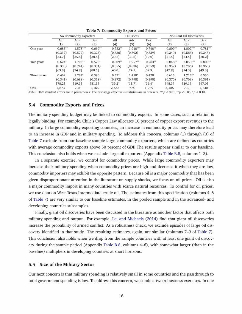
Table 7: Commodity Exports and PricesNo Commodity Exporters Oil Prices No Giant Oil Discoveries

All Adv. Dev. All Adv. Dev. All Adv. Dev.(1) (2) (3) (4) (5) (6) (7) (8) (9)

One year 0.686∗∗ 1.578∗∗∗ 0.669∗∗ 0.782∗∗ 1.918∗∗∗ 0.748∗∗ 0.809∗∗ 1.802∗∗∗ 0.781∗∗

(0.317) (0.572) (0.323) (0.336) (0.592) (0.339) (0.340) (0.566) (0.345)[33.7] [35.4] [38.4] [20.2] [33.6] [19.0] [21.4] [34.4] [20.2]

Two years 0.624∗ 1.703∗∗ 0.570∗ 0.809∗∗ 1.957∗∗ 0.763∗∗ 0.848∗∗ 2.053∗∗∗ 0.803∗∗

(0.330) (0.741) (0.334) (0.355) (0.836) (0.359) (0.357) (0.786) (0.360)[63.8] [24.7] [80.5] [40.0] [24.5] [39.9] [47.9] [24.3] [49.3]

Three years 0.462 1.287∗ 0.390 0.531 1.450∗ 0.470 0.615 1.715∗∗ 0.556(0.341) (0.688) (0.358) (0.372) (0.798) (0.390) (0.376) (0.763) (0.391)[78.2] [19.3] [81.5] [39.2] [18.7] [36.4] [48.3] [19.1] [47.0]

Obs. 1, 873 708 1, 165 2, 563 774 1,789 2, 485 755 1,730Notes: HAC standard errors are in parentheses. The first-stage effective F -statistics are in brackets. ∗∗∗p < 0.01, ∗∗p < 0.05, ∗p < 0.10.

5.4 Commodity Exports and Prices

The military-spending budget may be linked to commodity exports. In some cases, such a relation is

legally binding. For example, Chile’s Copper Law allocates 10 percent of copper export revenues to the

military. In large commodity-exporting countries, an increase in commodity prices may therefore lead

to an increase in GDP and in military spending. To address this concern, columns (1) through (3) of

Table 7 exclude from our baseline sample large commodity exporters, which are defined as countries

with average commodity exports above 50 percent of GDP. The results appear similar to our baseline.

This conclusion also holds when we exclude large oil exporters (Appendix Table B.8, columns 1–3).

In a separate exercise, we control for commodity prices. While large commodity exporters may

increase their military spending when commodity prices are high and decrease it when they are low,

commodity importers may exhibit the opposite pattern. Because oil is a major commodity that has been

given disproportionate attention in the literature on supply shocks, we focus on oil prices. Oil is also

a major commodity import in many countries with scarce natural resources. To control for oil prices,

we use data on West Texas Intermediate crude oil. The estimates from this specification (columns 4–6

of Table 7) are very similar to our baseline estimates, in the pooled sample and in the advanced- and

developing-countries subsamples.

Finally, giant oil discoveries have been discussed in the literature as another factor that affects both

military spending and output. For example, Lei and Michaels (2014) find that giant oil discoveries

increase the probability of armed conflict. As a robustness check, we exclude episodes of large oil dis-

covery identified in that study. The resulting estimates, again, are similar (columns 7–9 of Table 7).

This conclusion also holds when we drop from the sample countries with at least one giant oil discov-

ery during the sample period (Appendix Table B.8, columns 4–6), with somewhat larger (than in the

baseline) multipliers in developing countries at short horizons.

5.5 Size of the Military Sector

Our next concern is that military spending is relatively small in some countries and the passthrough to

total government spending is low. To address this concern, we conduct two robustness exercises. In one

16

Table 8: OLS EstimatesBaseline Adv. Dev. Rec. Exp. Peg Float Closed Open

(1) (2) (3) (4) (5) (6) (7) (8) (9)One year 0.494∗∗∗ 0.989∗∗∗ 0.482∗∗∗ 0.667∗∗∗ 0.236∗∗ 0.763∗∗∗ 0.383∗∗ 1.317∗∗∗ 0.342∗∗

(0.155) (0.378) (0.156) (0.188) (0.118) (0.122) (0.160) (0.353) (0.136)

Two years 0.612∗∗∗ 1.029∗∗ 0.602∗∗∗ 0.699∗∗∗ 0.294∗ 0.935∗∗∗ 0.418∗∗ 1.382∗∗∗ 0.442∗∗

(0.170) (0.455) (0.174) (0.192) (0.152) (0.156) (0.179) (0.351) (0.174)

Three years 0.558∗∗∗ 0.899∗ 0.555∗∗∗ 0.621∗∗∗ 0.246 0.926∗∗∗ 0.322 1.375∗∗∗ 0.379∗

(0.196) (0.505) (0.202) (0.195) (0.171) (0.170) (0.198) (0.356) (0.209)Notes: HAC standard errors are in parentheses. ∗∗∗p < 0.01, ∗∗p < 0.05, ∗p < 0.10.

exercise, we restrict the sample to countries with high shares of military spending (e.g., more than 5 or

10 percent of total spending). In the other, we drop from the sample countries for which an increase

in government spending, on average, did not lead to an increase in total spending (i.e., we focus on

cases with a positive correlation of changes in gm and g). To save space, the results are relegated to the

appendix (Tables B.9 and B.10). In both cases, there is little material effect on the multiplier.

5.6 OLS Estimates

Finally, it is instructive to compare our baseline IV estimates with those from ordinary least squares

(OLS). If government spending is used as a means of countercyclical fiscal policy, using total government

spending as a fiscal shock may result in attenuation bias. To the extent that military spending responds

only to geopolitical events unrelated to domestic economic conditions, and fiscal policy is effective, we

expect the OLS estimates to be smaller than the baseline IV estimates. As Table 8 suggests, this is indeed

the case, and in many samples the attenuation is quite large. The OLS estimates can also be interpreted

as the multipliers obtained from an annual bivariate VAR, with Cholesky decomposition and government

spending ordered last (i.e., not responding to output contemporaneously). While this approach has been

used widely with quarterly data (e.g., Blanchard and Perotti 2002; Ilzetzki, Mendoza, and Végh 2013),

it is hard to justify with annual data, since it is unlikely that government spending takes more than a

year to react to changes in output. This exercise, however, enhances our understanding of the baseline

results.

6 Discussion

As our paper studies a large panel of countries, our ability to extend the analysis to other variables

and methods is limited by available data. For example, in order to compare our identification with

other alternatives, such as the Blanchard and Perotti (2002) identification, we need quarterly data. We

would also like to gain a better understanding of how the implementation of fiscal policy influences its

effectiveness. In this section, we discuss these issues, focusing on small subsamples of countries with

more data.

17

6.1 Comparison with Ilzetzki et al.

Because Ilzetzki, Mendoza, and Végh (2013) use a different sample and different method, we strive

to explain the differences between their results and ours. While our results are, overall, qualitatively

similar to theirs, our point estimates are larger for both developed and developing countries. The

differences could be due to two factors: sample composition and identification.

To differentiate between these factors, we apply our method to a sample as close to theirs as possible.

We match their sample fairly well, with two exceptions: (1) our data for Australia, France, the United

Kingdom, and the United States start in 1988, while their data for France go back to 1978, and to 1960

for the other three countries; and (2) our sample does not include Iceland. In this exercise (Appendix

Table B.11), we obtain point estimates larger than in the baseline, but within the confidence intervals.

While these results point to the differences between the methodologies as a likely explanation, we

are cautious about this conclusion, due to remaining differences in the samples and, importantly, the

frequency of observations.

This exercise, in addition, confirms our earlier conjecture that the differences between advanced and

developing countries come mostly from low-income countries. Our multiplier estimates for developing

countries in the Ilzetzki et al. sample of mainly upper-middle-income countries are larger than the

baseline estimates and similar to those for developed countries, at least on impact.

6.2 Taxes

The effects of government spending on output may depend on, among other factors, whether the gov-

ernment spending is financed by taxes or debt. In the baseline, we estimate the size of the multiplier for

the average response of taxes in the sample. Distinguishing debt-financed government spending from

tax-financed spending is beyond the scope of this paper, due in part to a lack of available data. We

therefore address a more limited question: What is the response of tax rates to government-spending

shocks in countries with available tax data?

To this end, we collect data on tax rates from two sources. First, we use individual income marginal

tax rates from the OECD. These data provide information on the entire tax scale and personal allowances

for the member states. Second, to extend the coverage to developing countries, we use individual

income marginal tax rates of top earners from KPMG, an auditor. The KPMG data, however, provide

marginal tax rates for only the top income earners and are not available before 2006. While this measure

ignores variation in tax rates for low-income brackets as well as variation in personal allowance, it is

not affected by changes in total income or its distribution.

The left panel of Figure 3 shows that, while there is limited evidence that tax rates increase in re-

sponse to a spending shock at longer horizons, the increases are not statistically significant. When we

split the sample into advanced and developing countries (Appendix Figure B.6, Panel A), we find that,

in response to a spending shock, tax rates are more likely to increase in developing countries than in

developed ones. One potential explanation could be that developed countries have more capacity to

issue debt, whereas many developing-country governments operate in tight fiscal space. While confi-

18

Figure 3: Responses of Tax and Interest Rates to Military-Spending Shock

-8

-4

0

4

8

12

16Pe

rcen

t

1 2 3 4Years

Income tax

-6

-4

-2

0

2

4

Perc

enta

ge p

oint

s

1 2 3 4Years

Interest rate

Notes: The figure shows the IRFs of the income marginal tax rate (left panel) and the monetary-policy rate (right panel) to a military-spendingshock of 1 percent of GDP, estimated using the local projections method. The dashed lines represent one-standard-deviation bands, and thedotted lines show 95 percent confidence intervals.

dence intervals are large due to the small samples with available data, the difference in tax responses

is consistent with larger multipliers in advanced economies.

6.3 Monetary Policy

The size of the fiscal multiplier may also depend on whether the monetary authority leans against the

wind—and, if so, to what extent—as well as on the monetary-fiscal coordination. To get a sense of

whether monetary policy leaned against the wind in our sample, we estimate the responses of policy

rates to government-spending shocks. We obtain end-of-year policy rates for 25 countries and the euro

area, provided by the corresponding central banks. When official policy rates are not available, we use

discount rates from the IMF’s International Financial Statistics.

The right panel of Figure 3 suggests no statistically significant increases in interest rates at all hori-

zons considered. We also find little qualitative difference between the interest-rate responses in ad-

vanced and developing countries; both are negative and insignificant (Appendix Figure B.6, Panel B).

The responses in advanced countries are especially small quantitatively, which could be explained, in

part, by a prolonged period of the zero lower bound in our sample.

We provide additional evidence on the responses of output, policy rates, and taxes from a four-

variable panel VAR with shocks identified by ordering military spending last (and output first) in the

Cholesky decomposition (Appendix Figure B.7). The responses are consistent with our baseline evi-

dence. Since the data on policy rates and taxes are available mostly for advanced and upper-middle-

income countries, we re-estimate cumulative multipliers in the samples with data for each of the two

variables (Table B.12). Since we find multipliers larger than in the baseline, it is conceivable that the

responses of tax rates and policy rates in countries with no data were different.

19

Table 9: Sectoral Military Spending

(1) (2) (3) (4)Military nondurables 1.62∗∗

(0.66)Military durables 4.50∗∗∗ 2.91∗∗ 0.96

(1.11) (1.37) (1.76)

Total military spending 1.29∗∗ 1.26(0.66) (0.99)

Recession × Military durables 4.86∗∗

(2.43)

Recession × Total military spending −0.82(1.20)

Obs. 548 548 548 548

Notes: This table presents estimates of the one-year output response to military spend-ing on durables and on nondurables/services. Estimates of Equation (3) are in column(3). Standard errors are in parentheses. ∗∗∗p < 0.01, ∗∗p < 0.05, ∗p < 0.10.

6.4 Spending Composition

The effectiveness of government spending may also depend on spending composition (Ramey and

Shapiro 1998). One particular characteristic of spending composition discussed in the recent literature

is product durability (e.g., Boehm 2016). Using data on spending composition in, mostly, advanced

economies, we provide some evidence on the effects of spending on military durables and nondurables.

Following Gartzke (2001), we use data from NATO press releases and other sources, and define military

equipment and infrastructure as durables, and spending on personnel and other expenditures (typically,

operations costs) as spending on nondurables and services.

Since we do not have data on total government spending on durables and nondurables, we deviate

from our baseline methodology by instead estimating the direct contemporaneous response of output

to military spending, by type. Specifically, we estimate the following specification:

∆yi,t

yi,t−1= αi + β

∆gmi,t

yi,t−1+ ζ

∆gdi,t

yi,t−1+γγγzzz i,t + δt + εi,t , (3)

where gdi,t is government spending on military durables, and other variables and parameters are defined

as before. In this specification, a $1 increase in military spending on nondurables raises output by β

dollars, while $1 spent on durables raises it by (β+ζ) dollars. If there is no difference between the two

effects (i.e., ζ= 0), then β= µ1 (∂ g/∂ gm); in other words, β is close to the one-year multiplier as long

as the passthrough from military spending into total spending is close to one.

Table 9 shows estimates of the output response to military spending on durables and on non-

durables/services. In columns (1) and (2), we include one type of spending at a time, while column

(3) presents estimates of Equation (3) as a whole. The output effect of spending on military durables is

substantially larger than that on military nondurables. Our benchmark estimates in column (3) indicate

that a $1 increase in government spending on military nondurables and services is associated with a

$1.29 increase in output, while $1 spent on durables leads to an additional increase in output of $2.91.

While this difference is statistically significant, small coefficients are possible, and the effects of both

20

types of spending dissipate over longer horizons (Appendix Figure B.8).

Why is the output response to durables spending so large? In column (4), we interact the two vari-

ables with the recession dummy and find that the differences comes mostly from recessionary episodes.

Another potential reason is that large spending programs are often focused on durables, and large shocks

could be disproportionately more effective. We leave analyses of potential nonlinearities in the effects

of fiscal shocks to future research.

7 Conclusion

Using data on military spending for more than a hundred countries, we estimate an annual government-

spending multiplier, pooled across the sample, in the range 0.75–0.85. The multiplier estimates remain

significant over longer horizons. We also find that the multiplier is larger in developed countries than

in developing countries, under a fixed exchange rate than under a floating regime, in recessions than in

expansions, and in closed economies than in open economies. Hence, there is a wide range of economic

conditions for which expansionary fiscal policy can be a particularly effective stabilization tool.

These findings have important implications for policymakers, as the decisions on whether and how

to use fiscal policy should account for particular economic circumstances and environments. Our find-

ings also have implications for the identification of government-spending shocks. We find that the

military-shocks approach produces multipliers comparable to those from other methods and robust to

tests involving various controls and samples that could potentially violate the identifying assumption.

This paper also touches on three important issues that need further investigation but require addi-

tional data. While, for a subset of countries with available data, we do not find a strong response of

tax rates to government-spending shocks, we hope that, in future work, tax-financed multipliers will

be given further assessment. Next, we find only mild evidence of coordination between the fiscal and

monetary authorities, which may point to some institutional constraints. It remains a question if such

coordination can affect the multiplier size in a quantitatively important manner. Finally, the role of

spending composition as well as other aspects of fiscal programs can be explored further when more

data become available.

References

Aiyagari, S. Rao, Lawrence J. Christiano, and Martin Eichenbaum. 1992. “The Output, Employment, and InterestRate Effects of Government Consumption.” Journal of Monetary Economics 30(1): 73–86.

Alesina, Alberto, and Silvia Ardagna. 1998. “Tales of Fiscal Adjustment.” Economic Policy 13(27): 487–545.

Auerbach, Alan J., and Yuriy Gorodnichenko. 2012. “Measuring the Output Responses to Fiscal Policy.” AmericanEconomic Journal: Economic Policy 4(2): 1–27.

———. 2013. “Fiscal Multipliers in Recession and Expansion.” In Fiscal Policy after the Financial Crisis, edited byAlberto Alesina and Francesco Giavazzi, chap. 2, pp. 63–98. Chicago, IL: University of Chicago Press.

———. 2016. “Effects of Fiscal Shocks in a Globalized World.” IMF Economic Review 64(1): 177–215.

21

Ball, Nicole. 1988. Security and Economy in the Third World. Princeton, NJ: Princeton University Press.

Barro, Robert J. 1981. “Output Effects of Government Purchases.” Journal of Political Economy 89(6): 1086–1121.

Barro, Robert J., and Robert G. King. 1984. “Time-Separable Preferences and Intertemporal-Substitution Modelsof Business Cycles.” Quarterly Journal of Economics 99(4): 817–839.

Barro, Robert J., and Charles J. Redlick. 2011. “Macroeconomic Effects from Government Purchases and Taxes.”Quarterly Journal of Economics 126(1): 51–102.

Baxter, Marianne, and Robert G. King. 1993. “Fiscal Policy in General Equilibrium.” American Economic Review83(3): 315–334.

Beetsma, Roel, and Massimo Giuliodori. 2011. “The Effects of Government Purchases Shocks: Review and Esti-mates for the EU.” Economic Journal 121(550): 4–32.

Blanchard, Olivier, and Roberto Perotti. 2002. “An Empirical Characterization of the Dynamic Effects of Changesin Government Spending and Taxes on Output.” Quarterly Journal of Economics 117(4): 1329–1368.

Boehm, Christoph E. 2016. “Government Spending and Durable Goods.” Working paper, University of Texas,Austin, dropbox.com/s/cdhm6eof59o20f3/CBoehm_JMP.pdf.

Born, Benjamin, Falko Juessen, and Gernot J. Müller. 2013. “Exchange Rate Regimes and Fiscal Multipliers.”Journal of Economic Dynamics and Control 37(2): 446–465.

Broda, Christian, and Jonathan A. Parker. 2014. “The Economic Stimulus Payments of 2008 and the AggregateDemand for Consumption.” Journal of Monetary Economics 68(Suppl.): S20–S36.

Cacciatore, Matteo, and Nora Traum. 2018. “Trade Flows and Fiscal Multipliers.” Working paper, HEC Montréal,sites.google.com/site/cacciatm/ct_nber_2018_12_10.pdf.

Chodorow-Reich, Gabriel. 2018. “Geographic Cross-Sectional Fiscal Spending Multipliers: What Have WeLearned?” American Economic Journal: Economic Policy. Forthcoming.

Chodorow-Reich, Gabriel, Laura Feiveson, Zachary Liscow, and William G. Woolston. 2012. “Does State FiscalRelief during Recessions Increase Employment? Evidence from the American Recovery and Reinvestment Act.”American Economic Journal: Economic Policy 4(3): 118–145.

Christiano, Lawrence, Martin Eichenbaum, and Sergio Rebelo. 2011. “When Is the Government Spending Multi-plier Large?” Journal of Political Economy 119(1): 78–121.

Clemens, Jeffrey, and Stephen Miran. 2012. “Fiscal Policy Multipliers on Subnational Government Spending.”American Economic Journal: Economic Policy 4(2): 46–68.

Collier, Paul. 2006. “War and Military Expenditure in Developing Countries and Their Consequences for Devel-opment.” Economics of Peace and Security Journal 1(1): 10–13.

Corsetti, Giancarlo, André Meier, and Gernot J. Müller. 2012. “What Determines Government Spending Multipli-ers?” Economic Policy 27(72): 521–565.

Driscoll, John C., and Aart C. Kraay. 1998. “Consistent Covariance Matrix Estimation with Spatially DependentPanel Data.” Review of Economics and Statistics 80(4): 549–560.

Dupor, Bill, and Rodrigo Guerrero. 2017. “Local and Aggregate Fiscal Policy Multipliers.” Journal of MonetaryEconomics 92: 16–30.

Eggertsson, Gauti B. 2011. “What Fiscal Policy Is Effective at Zero Interest Rates?” In NBER MacroeconomicsAnnual 2010, vol. 25, edited by Daron Acemoglu and Michael Woodford, chap. 2, pp. 59–112. Chicago, IL:University of Chicago Press.

22

Eggertsson, Gauti B., and Michael Woodford. 2003. “The Zero Bound on Interest Rates and Optimal MonetaryPolicy.” Brookings Papers on Economic Activity 34(1): 139–235.

Fernández, Andrés, Michael W. Klein, Alessandro Rebucci, Martin Schindler, and Martín Uribe. 2016. “CapitalControl Measures: A New Dataset.” IMF Economic Review 64(3): 548–574.

Galí, Jordi, J. David López-Salido, and Javier Vallés. 2007. “Understanding the Effects of Government Spendingon Consumption.” Journal of the European Economic Association 5(1): 227–270.

Gartzke, Erik. 2001. “Democracy and the Preparation for War: Does Regime Type Affect States’ Anticipation ofCasualties?” International Studies Quarterly 45(3): 467–484.

Gavin, Michael, and Roberto Perotti. 1997. “Fiscal Policy in Latin America.” In NBER Macroeconomics Annual1997, vol. 12, edited by Ben S. Bernanke and Julio J. Rotemberg, chap. 1, pp. 11–72. Cambridge, MA: MITPress.

Gleditsch, Nils, Peter Wallensteen, Mikael Eriksson, Margareta Sollenberg, and Håvard Strand. 2002. “ArmedConflict 1946–2001: A New Dataset.” Journal of Peace Research 39(5): 615–637.

Gordon, Robert J., and Robert Krenn. 2010. “The End of the Great Depression 1939–41: Policy Contributions andFiscal Multipliers.” Working paper 16380, National Bureau of Economic Research.

Hagedorn, Marcus, Iourii Manovskii, and Kurt Mitman. 2019. “The Fiscal Multiplier.” Working paper 25571,National Bureau of Economic Research.

Hall, Robert E. 1986. “The Role of Consumption in Economic Fluctuations.” In The American Business Cycle:Continuity and Change, edited by Roger J. Gordon, chap. 4, pp. 237–266. Chicago, IL: University of ChicagoPress.

———. 2009. “By How Much Does GDP Rise If the Government Buys More Output?” Brookings Papers onEconomic Activity 40(2): 183–249.

House, Christopher L., and Matthew D. Shapiro. 2006. “Phased-In Tax Cuts and Economic Activity.” AmericanEconomic Review 96(5): 1835–1849.

Ilzetzki, Ethan, and Carlos A. Végh. 2008. “Procyclical Fiscal Policy in Developing Countries: Truth or Fiction?”Working paper 14191, National Bureau of Economic Research.

Ilzetzki, Ethan O., Enrique G. Mendoza, and Carlos A. Végh. 2013. “How Big (Small?) Are Fiscal Multipliers?”Journal of Monetary Economics 60(2): 239–254.

Johnson, David S., Jonathan A. Parker, and Nicholas S. Souleles. 2006. “Household Expenditure and the IncomeTax Rebates of 2001.” American Economic Review 96(5): 1589–1610.

Jordà, Òscar. 2005. “Estimation and Inference of Impulse Responses by Local Projections.” American EconomicReview 95(1): 161–182.

Klein, Michael W., and Jay C. Shambaugh. 2008. “The Dynamics of Exchange Rate Regimes: Fixes, Floats, andFlips.” Journal of International Economics 75(1): 70–92.

Kraay, Aart. 2012. “How Large Is the Government Spending Multiplier? Evidence from World Bank Lending.”Quarterly Journal of Economics 127(2): 829–887.

———. 2014. “Government Spending Multipliers in Developing Countries: Evidence from Lending by OfficialCreditors.” American Economic Journal: Macroeconomics 6(4): 170–208.

Lei, Yu-Hsiang, and Guy Michaels. 2014. “Do Giant Oilfield Discoveries Fuel Internal Armed Conflicts?” Journalof Development Economics 110(C): 139–157.

23

Leigh, Daniel, Pete Devries, Charles Freedman, Jaime Guajardo, Douglas Laxton, and Andrea Pescatori. 2010.“Will It Hurt? Macroeconomic Effects of Fiscal Consolidation.” In World Economic Outlook: Recovery, Risk, andRebalancing, chap. 3, pp. 93–124. Washington, DC: International Monetary Fund.

Mertens, Karel, and Morten O. Ravn. 2012. “Empirical Evidence on the Aggregate Effects of Anticipated andUnanticipated US Tax Policy Shocks.” American Economic Journal: Economic Policy 4(2): 145–181.

Michaillat, Pascal. 2014. “A Theory of Countercyclical Government Multiplier.” American Economic Journal:Macroeconomics 6(1): 190–217.

Miyamoto, Wataru, Thuy Lan Nguyen, and Viacheslav Sheremirov. 2019. “The Effects of Government Spendingon Real Exchange Rates: Evidence from Military Spending Panel Data.” Journal of International Economics 116:144–157.

Montiel Olea, José Luis, and Carolin Pflueger. 2013. “A Robust Test for Weak Instruments.” Journal of Business &Economic Statistics 31(3): 358–369.

Mundell, Robert A. 1963. “Capital Mobility and Stabilization Policy under Fixed and Flexible Exchange Rates.”Canadian Journal of Economics and Political Science 29(4): 475–485.

Nakamura, Emi, and Jón Steinsson. 2014. “Fiscal Stimulus in a Monetary Union: Evidence from US Regions.”American Economic Review 104(3): 753–792.

Parker, Jonathan A. 2011. “On Measuring the Effects of Fiscal Policy in Recessions.” Journal of Economic Literature49(3): 703–718.

Parker, Jonathan A., Nicholas S. Souleles, David S. Johnson, and Robert McClelland. 2013. “Consumer Spendingand the Economic Stimulus Payments of 2008.” American Economic Review 103(6): 2530–2553.

Perotti, Roberto. 2008. “In Search of the Transmission Mechanism of Fiscal Policy.” In NBER MacroeconomicsAnnual 2007, vol. 22, edited by Daron Acemoglu, Kenneth S. Rogoff, and Michael Woodford, chap. 3, pp. 169–226. Chicago, IL: University of Chicago Press.

Ramey, Valerie A. 2011a. “Can Government Purchases Stimulate the Economy?” Journal of Economic Literature49(3): 673–685.

———. 2011b. “Identifying Government Spending Shocks: It’s All in the Timing.” Quarterly Journal of Economics126(1): 1–50.

Ramey, Valerie A., and Matthew D. Shapiro. 1998. “Costly Capital Reallocation and the Effects of GovernmentSpending.” Carnegie-Rochester Conference Series on Public Policy 48(1): 145–194.

Ramey, Valerie A., and Sarah Zubairy. 2018. “Government Spending Multipliers in Good Times and in Bad:Evidence from US Historical Data.” Journal of Political Economy 126(2): 850–901.

Reinhart, Carmen, and Kenneth Rogoff. 2011. “From Financial Crash to Debt Crisis.” American Economic Review101(5): 1676–1706.

Romer, Christina D., and David H. Romer. 2010. “The Macroeconomic Effects of Tax Changes: Estimates Basedon a New Measure of Fiscal Shocks.” American Economic Review 100(3): 763–801.

Rotemberg, Julio J., and Michael Woodford. 1992. “Oligopolistic Pricing and the Effects of Aggregate Demandon Economic Activity.” Journal of Political Economy 100(6): 1153–1207.

Sarkees, Meredith R., and Frank Wayman. 2010. Resort to War: 1816–2007. Washington, DC: CQ Press.

Shoag, Daniel. 2015. “The Impact of Government Spending Shocks: Evidence on the Multiplier from State PensionPlan Returns.” Working paper, Harvard University,scholar.harvard.edu/files/shoag/files/impact_of_government_spending_shocks_01.pdf.

24

Staiger, Douglas, and James H. Stock. 1997. “Instrumental Variables Regression with Weak Instruments.” Econo-metrica 65(3): 557–586.

Suárez Serrato, Juan Carlos, and Philippe Wingender. 2016. “Estimating Local Fiscal Multipliers.” Working paper22425, National Bureau of Economic Research.

Talvi, Ernesto, and Carlos A. Végh. 2005. “Tax Base Variability and Procyclical Fiscal Policy in Developing Coun-tries.” Journal of Development Economics 78(1): 156–190.

Woodford, Michael. 2011. “Simple Analytics of the Government Expenditure Multiplier.” American EconomicJournal: Macroeconomics 3(1): 1–35.

25

Appendix

A Data Sources

Annual data on real GDP, government spending, and military spending are available for 160 countries during theperiod 1988–2013: 3,298 observations in total. We use the number of years for which these variables are availableto proxy for the reliability of the data for a particular country. For this reason, we exclude 31 countries that havefewer than 15 years of observations.1 These inclusion criteria also weed out countries that had significant wars ondomestic soil, such as Afghanistan and Iraq, leaving us with a sample of relatively stable countries.

Our final sample contains 129 countries (36 advanced and 93 developing): 3,001 observations in total. Ta-ble A.1 contains information on the countries available in the entire sample, as well as the number of observationsavailable per country. In what follows, we provide a short summary of the data and sources used in our analysis.

Real GDP and Total Government Spending: We obtain annual data on real GDP and general-government finalconsumption expenditure, at constant 2005 prices in national-currency units, from the National Accounts Main Ag-gregates Database, provided by the U.N. Statistics Division. The dataset contains time-series from 1970 onward formore than 200 countries, which report to the United Nations in the form of the National Accounts Questionnaires.We use the December 2014 version of the dataset, which has data available until 2013. For additional informationand detailed methodology, see unstats.un.org/unsd/snaama/index.

Total Military Spending: Stockholm International Peace Research Institute (SIPRI) provides data on total mili-tary expenditure for 171 countries in the period 1988–2013. SIPRI collects data from three sources: (1) nationalgovernments and statistical agencies; (2) international organizations (e.g., NATO press releases, IMF country re-ports); and (3) specialist newspapers, journals, and other publications (e.g., Economist Intelligence Unit, EuropaWorld). We calculate total military spending by using the ratios of military spending to GDP. More specifically, wemultiply these ratios by real GDP, obtained from the United Nations, to calculate total military spending at constant2005 prices in national-currency units. For more details, see sipri.org/research/armaments/milex/milex_database.

Development Classification: The development classifications are taken from the IMF and World Bank. TheWorld Bank classification is based on gross national income. More information can be found atdatahelpdesk.worldbank.org/knowledgebase/articles/378834-how-does-the-world-bank-classify-countries.

Unemployment Rates: We obtain unemployment data from the World Bank’s World Development Indicators(WDI) database. We use the October 2015 edition of the database. The coverage starts in 1991. The WorldBank collects the unemployment series from the International Labor Organization. More information can be foundat datacatalog.worldbank.org/dataset/world-development-indicators.

Exchange-Rate Regimes: The exchange-rate classification follows Klein and Shambaugh (2008), updated to2013. A country is considered to have a fixed exchange rate if the end-of-month exchange rate stays within the2 percent bands for the entire year. The updated classification can be found at gwu.edu/∼iiep/about/faculty/jshambaugh/data.cfm.

Trade: We use data on exports and imports of goods and services as a percentage of GDP from the WDI. Theexports and imports series are collected from the World Bank and the OECD national accounts data. These seriesexclude compensation of employees, investment income, and transfer payments. We use these data to create an

1The countries excluded are Afghanistan, Benin, Bosnia and Herzegovina, Central African Republic, Congo-Brazzaville, DemocraticRepublic of the Congo, Equatorial Guinea, Eritrea, Gabon, Gambia, Guinea, Guinea-Bissau, Haiti, Honduras, Iceland, Iraq, Kuwait, Liberia,Libya, Montenegro, Niger, Panama, Qatar, South Sudan, Tajikistan, Timor Leste, Togo, Trinidad and Tobago, Turkmenistan, Uzbekistan, andZimbabwe.

i

Table A.1: Countries in the SampleCountry Obs. cont.Albania 21Algeria 25 Lebanon 23Angola 20 Lesotho 25Argentina 25 Lithuania 20Armenia 19 Luxembourg 25Australia 25 Macedonia 17Austria 25 Madagascar 25Azerbaijan 21 Malawi 23Bahrain 25 Malaysia 25Bangladesh 25 Mali 22Belarus 21 Malta 25Belgium 25 Mauritania 19Belize 23 Mauritius 25Bolivia 24 Mexico 25Botswana 25 Moldova 20Brazil 25 Mongolia 22Brunei 25 Morocco 25Bulgaria 24 Mozambique 22Burkina Faso 25 Namibia 23Burundi 21 Nepal 25Cambodia 25 Netherlands 25Cameroon 25 New Zealand 25Canada 25 Nicaragua 23Cape Verde 19 Nigeria 25Chad 16 Norway 25Chile 25 Oman 25China 24 Pakistan 25Colombia 25 Papua New Guinea 25Côte d’Ivoire 16 Paraguay 24Croatia 21 Peru 24Cyprus 25 Philippines 25Czech Republic 20 Poland 25Denmark 25 Portugal 25Djibouti 20 Romania 25Dominican Republic 25 Russia 21Ecuador 25 Rwanda 25Egypt 25 Saudi Arabia 25El Salvador 25 Senegal 22Estonia 21 Serbia 16Ethiopia 23 Seychelles 25Fiji 25 Sierra Leone 22Finland 25 Singapore 25France 25 Slovakia 20Georgia 17 Slovenia 21Germany 25 South Africa 25Ghana 25 Spain 25Greece 25 Sri Lanka 25Guatemala 25 Swaziland 25Guyana 21 Sweden 25Hungary 25 Switzerland 25India 25 Syria 22Indonesia 23 Tanzania 25Iran 24 Thailand 25Ireland 25 Tunisia 25Israel 25 Turkey 25Italy 25 United Arab Emirates 15Jamaica 24 Uganda 25Japan 25 Ukraine 20Jordan 25 United Kingdom 25Kazakhstan 20 United States 25Kenya 25 Uruguay 25Korea 25 Venezuela 22Kyrgyzstan 21 Vietnam 16Laos 20 Yemen 20Latvia 20 Zambia 18

ii

indicator for open and closed economies. We define an economy as open if its combined exports and imports sharesof GDP are greater than 60 percent.

Wars: The war data come from two sources: the Correlates of War project and the UCDP/PRIO Armed ConflictDataset. The war data contain information on participating countries, start and end dates, and the number of battledeaths for each conflict. For more information on the first source, see Sarkees and Wayman (2010). The datasetand its description are available at correlatesofwar.org/data-sets/COW-war. For more information on the secondsource, see Gleditsch et al. (2002) and prio.org/Data/Armed-Conflict/UCDP-PRIO.

Financial Crises: Annual data on financial crises come from Reinhart and Rogoff (2011). These data are availablefrom 1800 to 2010 for 70 countries and include information on crises pertaining to currency, inflation, stock market,sovereign debt, and banking. We consider a country to be in a financial crisis if it experiences any of these crises.See carmenreinhart.com/data/browse-by-topic/topics/7.

Democracy and Political Risk: The Polity IV Project provides classification of political regimes for 167 countriessince 1800. The dataset includes indicators for democracy, autocracy, regime durability, and polity persistency, aswell as other component variables related to the executive recruitment processes and the independence of exec-utive authority. The democracy and autocracy indicators range from zero to ten, with a score of ten indicating afull democracy or full autocracy, respectively. These indicators are calculated as the sum of the various authoritycharacteristic component variables. See systemicpeace.org/polityproject.html for more detail. We define a countryas an autocracy in a given year if the democracy index is smaller than the autocracy index. According to this defi-nition, a country can have a positive autocracy score and still be considered a democracy. We observe a maximumautocracy score of three among the countries we label as democratic.

We also use annual data on political stability and good governance from the World Bank’s Worldwide GovernanceIndicators (WGI). WGI reports governance indicators for over 200 countries since 1996. There are six indicatorsexpressed in standard normal units or percentile ranks: (1) voice and accountability, (2) political stability andabsence of violence/terrorism, (3) government effectiveness, (4) regulatory quality, (5) rule of law, and (6) controlof corruption. In our robustness checks, we use percentile ranks for political stability and government effectiveness.See info.worldbank.org/governance/wgi/#home. Note that while these two measures are different from those inMiyamoto, Nguyen, and Sheremirov (2019), those data are proprietary and therefore cannot be used freely tocompare the two measures.

Arms Imports: We collect annual data on arms trade from the U.S. Department of State’s World Military Expendi-tures and Arms Transfers. The data are available from 1964 onward for over 180 countries and provide informationon military expenditures, armed forces, arms imports, arms exports, and the number of weapons delivered. Seestate.gov/t/avc/rls/rpt/wmeat.

Commodities: Data on commodity exports are collected from the United Nations’ UNCTAD statistics and Com-trade database. The data can be found at unctad.org/en/pages/statistics.aspx and comtrade.un.org, respectively.We also use West Texas Intermediate crude oil prices. Data on giant oil discoveries come from Lei and Michaels(2014), who use data compiled by Myron Horn and the American Association of Petroleum Geologists. Thesedata are available for 193 countries from 1946 through 2008. A giant oil discovery is defined as an oilfield thatcontained ultimate recoverable reserves of at least 500 million barrels of oil.

Marginal Tax Rates: The OECD Central Government Personal Income Tax Rates and Thresholds dataset providesannual data on marginal income tax rates for 33 member countries for the period 1981–2014. We use the topmarginal income tax rate. See oecd.org/tax/tax-policy/tax-database.htm. In addition, we use marginal incometax rates provided by KPMG, an auditor. The KPMG data include tax rates for both advanced and developingcountries for the period 2006–2014. While the KPMG data also include tax rates for developed countries, theperiod covered is shorter than that in the OECD data. See home.kpmg/mm/en/home/services/tax/tax-tools-and-resources/tax-rates-online/individual-income-tax-rates-table.html.

iii

Monetary Policy Rates: We collect end-of-period interest rate data for 75 countries (36 advanced and 39 de-veloping). The data, starting in 1960 for some countries, were obtained from the IMF’s International FinancialStatistics (IFS) and national central banks. See data.imf.org/IFS.

Disaggregated Military Spending: Data on the composition of military spending come from Gartzke (2001) andNATO. Gartzke’s data are available from 1950 through 1997 for 99 countries, but the coverage is incomplete. Thedata are split into capital and operating costs in constant U.S. dollars, which proxy for durable and nondurablespending. The data come from four sources: (1) NATO press releases, (2) The UN Report on Military Expenditures,(3) SIPRI Yearbook, and (4) Ball (1988). For several countries, there are two observations for the same year. In suchcases, our preferred sources are SIPRI and NATO, and our third preferred source is the United Nations. Becausethe Gartzke (2001) data end in 1997, we supplement them with those from NATO for the period 1998–2013, usinghis method. See nato.int/cps/en/natohq/topics_49198.htm for data details. To calculate durable and nondurablespending in constant 2005 prices in local currency units, we multiply the durable and nondurable shares by totalmilitary spending. The resulting series covers 53 countries, mostly NATO members.

iv

B Additional Results

Figure B.1: Time and Space Distributions of Main Variables

0

5

10

15

20

25

30

Perc

ent

-40 -20 0 20 40Change on previous year, %

Military spending

0

5

10

15

20

25

30

Perc

ent

-40 -20 0 20 40Change on previous year, %

Total government spending

0

5

10

15

20

25

30

Perc

ent

-40 -20 0 20 40Change on previous year, %

Output

-40

-20

0

20

40

Ave

rage

cha

nge,

%

1990

1995

20002005

20102015

Year

-40

-20

0

20

40

Ave

rage

cha

nge,

%

1990

1995

20002005

20102015

Year

-40

-20

0

20

40

Ave

rage

cha

nge,

%19

9019

952000

20052010

2015

Year

Notes: The top three panels show the distribution of changes, in percent, in military spending, total government spending, and output,respectively. For readability, changes over 40 percent in absolute value are cut off. The bottom three panels show the averages (black solidline) and medians (red broken line, virtually indistinguishable) of corresponding changes by year. The dashed lines depict one standarddeviation around the averages.

Table B.1: Distribution of |∆ ln gm| over Countries

Average year Median year(1) (2)

Mean 0.115 0.081Standard deviation 0.063 0.044Minimum 0.028 0.018Maximum 0.425 0.250Percentiles:

10th 0.044 0.03525th 0.069 0.05050th 0.104 0.07175th 0.148 0.10390th 0.192 0.136

United States 0.053 0.044Larger than U.S. share 0.853 0.814

Notes: We compute annual log-changes in military spending,∆ ln gm

i,t = ln gmi,t−ln gm

i,t−1 and then, in column (1), report the mean,standard deviation, and percentiles of its average (over time) abso-lute value, |∆ ln gm

i | =∑

t |∆ ln gmi,t |/T , across countries (i). In col-

umn (2), we report the moments and percentiles for medians ratherthan averages over time. The penultimate row reports the corre-sponding measure for the U.S., and the last row reports the share ofcountries (between 0 and 1) with |∆ ln gm

i |> |∆ ln gmU.S.|.

v

Figure B.2: Comovement of Military Spending Shocks in the United States with the Rest of the World (RoW)

Correlation = 0.40

-2

-1

0

1

2

Stan

dard

ized

sho

cks

1990

1995

2000 2005

2010

United StatesAverage across RoW

Notes: The figure depicts military spending shocks obtained as the fitted values from the regression of the log-difference of total governmentspending on the log-difference of military spending. To enhance visibility, the shocks are standardized (demeaned and divided by thestandard deviation over time).

Figure B.3: Correlation of Total Government Spending with Military Spending across Countries

0

5

10

15

20

25

Num

ber

of c

ount

ries

-.8 -.6 -.4 -.2 0 .2 .4 .6 .8 1Corr(∆ln gm, ∆ln g)

Notes: For each country i, we compute time correlation of log changes in military spending and log changes in total government spending,Corri(∆ ln gm

i,t ,∆ ln gi,t). This figure shows the histogram of Corri over i. The blue and red colors indicate positive and negative values ofCorri , respectively. In 103 out of 129 countries, the sample correlation is positive.

vi

Table B.2: Sensitivity to the Number of Lags

One lag Two lags Three lags Four lags(1) (2) (3) (4)

One year 0.643 0.725∗∗ 0.841∗∗∗ 0.833∗∗

(0.399) (0.356) (0.322) (0.330)[6.5] [6.3] [27.6] [23.0]

Two years 0.861∗ 0.832∗∗ 0.987∗∗ 0.879∗∗

(0.511) (0.401) (0.390) (0.366)[10.6] [9.4] [37.8] [39.7]

Three years 0.616 0.588 0.825∗∗ 0.649∗

(0.512) (0.378) (0.420) (0.390)[15.5] [12.2] [38.4] [36.0]

Four years 0.675 0.665 0.843∗ 0.656(0.611) (0.444) (0.487) (0.452)[10.2] [8.2] [32.3] [30.5]

Five years 0.474 0.466 0.750 0.509(0.619) (0.436) (0.555) (0.501)[15.1] [12.1] [25.0] [22.9]

Obs. 2,989 2,843 2,701 2,563

Notes: This table presents multipliers for alternative numbers of lags; the base-line includes four lags. HAC standard errors are in parentheses. First-stage ef-fective F -statistics are in brackets. The war dummy, country fixed effects, andtime effects are included. ∗∗∗p < 0.01, ∗∗p < 0.05, ∗p < 0.10.

Table B.3: Alternative Normalization: Lag Output

Fixed effects No Country (C) Time (T) C–T(1) (2) (3) (4)

One year 0.790∗∗ 0.795∗∗ 0.863∗∗ 0.889∗∗

(0.340) (0.383) (0.350) (0.396)[28.4] [23.6] [28.5] [23.5]

Two years 0.877∗∗ 0.881∗ 0.952∗∗ 0.990∗∗

(0.413) (0.472) (0.422) (0.482)[45.4] [35.5] [45.9] [36.0]

Three years 0.947∗ 0.963 1.042∗∗ 1.102∗

(0.507) (0.603) (0.520) (0.620)[51.8] [35.8] [52.6] [36.5]

Four years 1.051∗ 1.156 1.160∗∗ 1.359∗

(0.567) (0.721) (0.581) (0.737)[48.3] [31.0] [49.7] [32.3]

Five years 1.045 1.073 1.157∗ 1.354(0.648) (0.909) (0.657) (0.912)[42.3] [22.8] [43.5] [24.1]

Notes: This table presents multipliers based on an alternative variable transfor-mation. In this exercise, we normalize output, government spending, and mili-tary spending by lag output, as opposed to trend output. HAC standard errors arein parentheses. First-stage effective F -statistics are in brackets. The war dummy,country fixed effects, and time effects are included. ∗∗∗p < 0.01, ∗∗p < 0.05, ∗p <0.10.

vii

Table B.4: Alternative Standard Errors

One year Two years Three years Four years Five years(1) (2) (3) (4) (5)

Cumulative multiplier 0.833 0.879 0.649 0.656 0.509Errors:

Classical (0.122)∗∗∗ (0.160)∗∗∗ (0.220)∗∗∗ (0.274)∗∗ (0.337)Robust (0.322)∗∗∗ (0.341)∗∗ (0.377)∗ (0.436) (0.499)Heteroskedastic and autocorrelated (HAC) (0.330)∗∗ (0.366)∗∗ (0.390)∗ (0.452) (0.501)Clustered by country (0.380)∗∗ (0.399)∗∗ (0.409) (0.496) (0.540)Driscoll and Kraay (1998) (0.406)∗ (0.440)∗ (0.468) (0.521) (0.551)Two-way clustered by country and year (0.419)∗ (0.472)∗ (0.500) (0.594) (0.663)

Notes: This table presents the sensitivity of standard-errors estimates; the baseline uses HAC standard errors. The war dummy, coun-try fixed effects, and time effects are included. ∗∗∗p < 0.01, ∗∗p < 0.05, ∗p < 0.10.

Table B.5: Breakdown of Developing Sample

High income Less developedAll Middle income Low income

(1) (2) (3) (4)One year 2.022∗∗ 0.802∗∗ 1.885∗∗∗ 0.406

(0.938) (0.348) (0.715) (0.388)[4.7] [29.0] [19.7] [41.5]

Two years 1.778∗∗ 0.809∗∗ 1.886∗∗ 0.275(0.738) (0.374) (0.747) (0.438)[17.4] [44.9] [15.1] [53.6]

Three years 0.072 0.676∗ 1.575∗∗ 0.086(1.469) (0.395) (0.674) (0.547)[3.6] [47.5] [14.9] [39.9]

Obs. 701 1,861 1, 293 566

Notes: This table uses the World Bank development classification, based on gross nationalincome, which allows breaking down the developing sample further. Column (1) showsthe results for high-income (advanced) countries, and column (2) for less developed coun-tries (low- and middle-income countries together). Column (3) shows the results for upper-middle- and lower-middle-income countries (called middle-income for our purposes), whilecolumn (4) shows results for low-income countries.

viii

Figure B.4: IRFs to Military-Spending Shock in Advanced and Developing CountriesPanel A: Advanced Countries

0

1

2Pe

rcen

t

1 2 3 4 5Years

Output

0

1

2

Perc

ent o

f GD

P

1 2 3 4 5Years

Government spending

Panel B: Developing Countries

-1

0

1

2

Perc

ent

1 2 3 4 5Years

Output

-1

0

1

2

Perc

ent o

f GD

P

1 2 3 4 5Years

Government spending

Notes: The figure presents the impulse-response function (IRF) separately for advanced and developing countries. See notes to Figure 2.

ix

Figure B.5: IRFs to Military-Spending Shock by Development–Exchange Regime Sample

-1

0

1

2Pe

rcen

t of G

DP

1 2 3 4 5Years

OutputGovernment spending

Advanced, peg

-1

0

1

2

Perc

ent o

f GD

P

1 2 3 4 5Years

Developing, peg

-1

0

1

2

Perc

ent o

f GD

P

1 2 3 4 5Years

Advanced, float

-1

0

1

2

Perc

ent o

f GD

P

1 2 3 4 5Years

Developing, float

Notes: The figure presents the IRF by sample. The bands show one standard deviation around the estimates.

Table B.6: Multipliers during Slack Episodes: Alternative Thresholds

Unemployment threshold: percentile50th 75th 90th

High Low High Low High Low(1) (2) (3) (4) (5) (6)

One year 1.453∗∗∗ 0.771∗ 1.412∗∗ 0.893∗∗∗ 1.686∗∗ 0.754∗∗

(0.463) (0.443) (0.583) (0.339) (0.819) (0.309)[27.4] [15.3] [15.0] [23.0] [9.2] [27.1]

Two years 1.220∗∗ 0.958∗ 0.974 1.077∗∗∗ 1.205 0.846∗∗

(0.505) (0.490) (0.608) (0.380) (0.801) (0.357)[16.5] [59.8] [13.0] [52.9] [8.0] [48.4]

Three years 0.819 0.772 0.348 1.072∗∗ 0.671 0.672(0.515) (0.733) (0.671) (0.507) (0.831) (0.445)[12.5] [19.5] [13.0] [29.6] [7.5] [28.2]

Obs. 1, 306 1,218 659 1, 865 325 2, 199

Notes: The tables presents multipliers for alternative definitions of slack. The first two columns are the baseline,defined as the unemployment rate above the country’s median. The other four columns experiment with largerthresholds.

x

Table B.7: Multipliers and Wars

Military threat Excluding countries Excluding countriesindicator with long civil wars with any war incidence

(1) (2) (3)One year 0.779∗∗ 0.667∗∗ 1.068∗∗∗

(0.338) (0.308) (0.404)[19.6] [16.0] [48.7]

Two years 0.798∗∗ 0.728∗∗ 1.034∗∗∗

(0.359) (0.355) (0.393)[38.8] [32.3] [33.4]

Three years 0.529 0.478 0.836∗∗

(0.376) (0.372) (0.366)[37.5] [32.0] [30.5]

Obs. 2, 563 2,175 1, 377

Notes: In column (1), we control for a military-threat indicator based on the incidence of warin a narrowly defined geographical region. In column (2), we exclude countries with long civilwars (fought on domestic soil). In column (3), we exclude countries with any incidence of warduring the sample period.

Table B.8: Large Oil Exporters and Discoveries

No Large Oil Exporters No Countries with Giant Oil DiscoveriesAll Adv. Dev. All Adv. Dev.(1) (2) (3) (4) (5) (6)

One year 0.792∗∗ 1.569∗∗∗ 0.775∗∗ 1.315∗∗∗ 1.794∗∗∗ 1.270∗∗∗

(0.345) (0.570) (0.351) (0.449) (0.632) (0.492)[31.0] [36.0] [33.7] [22.9] [32.5] [18.8]

Two years 0.768∗∗ 1.693∗∗ 0.728∗ 1.228∗∗∗ 1.921∗∗ 1.167∗∗

(0.372) (0.740) (0.377) (0.436) (0.868) (0.472)[50.4] [25.2] [57.8] [36.8] [20.1] [36.5]

Three years 0.597 1.301∗ 0.546 0.905∗∗ 1.589∗ 0.834∗

(0.390) (0.695) (0.409) (0.440) (0.832) (0.474)[53.0] [19.5] [52.8] [34.8] [16.0] [35.9]

Obs. 2, 407 752 1,655 1, 780 519 1,261

Notes: In columns (1) through (3), we exclude countries with a share of oil exports in total exports above 15 per-cent of GDP: Algeria, Chile, Mauritania, Nigeria, Oman, Russia, Saudi Arabia, United Arab Emirates, and Zambia. Incolumns (4) through (6), we drop countries with at least one giant oil discovery in the sample.

xi

Table B.9: Relative Size of Military Spending

Share of military spendingBaseline > 5% > 10%

(1) (2) (3)One year 0.833∗∗ 0.864∗∗∗ 0.773∗∗

(0.330) (0.329) (0.318)[23.0] [23.9] [24.7]

Two years 0.879∗∗ 0.917∗∗ 0.799∗∗

(0.366) (0.363) (0.349)[39.7] [40.0] [42.6]

Three years 0.649∗ 0.697∗ 0.495(0.390) (0.388) (0.373)[36.0] [34.2] [34.5]

Four years 0.656 0.702 0.470(0.452) (0.450) (0.442)[30.5] [28.6] [27.6]

Five years 0.509 0.585 0.308(0.501) (0.496) (0.495)[22.9] [22.1] [20.3]

Obs. 2,563 2,354 1, 612

Notes: This table reproduces the baseline results for the cases whenwe drop countries with an average share of military spending in to-tal government spending below 5 percent (column 2) or below 10percent (column 3).

Table B.10: Excluding Countries with Corr (∆ ln gm,∆ ln g)≤ 0

Fixed effects No Country (C) Time (T) C–T(1) (2) (3) (4)

One year 0.702∗∗∗ 0.715∗∗ 0.759∗∗∗ 0.785∗∗

(0.266) (0.294) (0.271) (0.305)[30.5] [26.1] [30.4] [26.2]

Two years 0.736∗∗∗ 0.713∗∗ 0.785∗∗∗ 0.810∗∗

(0.278) (0.324) (0.280) (0.334)[59.1] [48.0] [58.7] [49.0]

Three years 0.557∗∗ 0.412 0.622∗∗ 0.598∗

(0.271) (0.335) (0.272) (0.349)[68.6] [48.4] [67.2] [50.6]

Four years 0.550∗ 0.378 0.633∗∗ 0.661(0.283) (0.396) (0.285) (0.412)[62.6] [39.0] [61.9] [42.6]

Five years 0.453 0.217 0.548∗ 0.578(0.295) (0.453) (0.292) (0.459)[52.9] [27.4] [52.4] [30.9]

Obs. 2,022 2,022 2,022 2,022

Notes: To construct this table, we drop countries with a negative sample correla-tion of changes in military spending and changes in total government spending.The distribution of these correlations across countries can be found in Figure B.3.

xii

Table B.11: Ilzetzki et al. Sample

All Adv. Dev.(1) (2) (3)

One year 2.179∗∗ 2.155 2.519∗

(1.002) (1.434) (1.463)[40.0] [27.3] [14.7]

Two years 2.050∗∗ 2.654∗ 1.733(1.018) (1.570) (1.350)[33.2] [18.8] [18.2]

Three years 1.991∗ 2.633 1.720(1.128) (1.628) (1.518)[19.7] [10.3] [11.7]

Obs. 823 524 299

Notes: This table presents multipliers estimated in the sample re-stricted to countries considered in Ilzetzki, Mendoza, and Végh(2013), except Iceland (not in our baseline sample). The datafor Australia, France, the United Kingdom, and the United Statesstart in 1988.

Figure B.6: Income Tax and Interest Rate Response to Government-Spending Shock by Country SamplePanel A: Income tax

-15

-10

-5

0

5

10

15

Perc

ent

1 2 3Years

Advanced economies

centering

-15

-10

-5

0

5

10

15

Perc

ent

1 2 3Years

Developing countries

Panel B: Interest rate

-1.0

-0.8

-0.6

-0.4

-0.2

0.0

0.2

0.4

0.6

0.8

1.0

Perc

enta

ge p

oint

s

1 2 3Years

Advanced economies

-6

-4

-2

0

2

Perc

enta

ge p

oint

s

1 2 3Years

Developing countries

Notes: The figure reproduces Figure 3 in the text, splitting the country sample into developed and developing countries. The dashed linesrepresent one standard deviation bands.

xiii

Figure B.7: IRFs to Military-Spending Shocks: VAR Estimates

-.5

0

.5

1

1.5

2

Perc

ent

1 2 3 4Years

Output

-.1

-.05

0

.05

.1

Perc

ent

1 2 3 4Years

Tax

-.1

-.05

0

.05

.1

Perc

ent

1 2 3 4Years

Interest rate

Notes: The figure presents impulse responses of output, marginal income tax rates, and policy rates to a military spending shock of 1 percentof GDP, estimated from a vector autoregression (VAR) with two lags. The system is identified using Cholesky decomposition, with militaryspending ordered last and output first (i.e., military spending does not respond to any variable within a year). Dotted lines represent 95percent confidence bands from Monte Carlo simulations.

Table B.12: Multipliers in Subsamples with Extra Data

Fixed effects No Country (C) Time (T) C–T(1) (2) (3) (4)Panel A: Tax-rate sample

One year 1.296∗∗∗ 1.376∗∗∗ 1.404∗∗∗ 1.509∗∗∗

(0.298) (0.301) (0.422) (0.391)[9.2] [8.5] [9.0] [8.1]

Two years 1.441∗∗∗ 1.353∗∗∗ 1.434∗∗∗ 1.421∗∗∗

(0.268) (0.298) (0.367) (0.399)[21.2] [17.2] [21.0] [18.0]

Three years 0.840∗∗∗ 0.639∗∗ 0.762∗∗ 0.739∗∗

(0.282) (0.286) (0.315) (0.311)[20.5] [38.3] [19.3] [38.8]

Obs. 1, 009 1,008 1,009 1,008Panel B: Policy-rate sample

One year 1.829∗∗ 1.930∗∗∗ 2.342∗∗∗ 2.382∗∗∗

(0.717) (0.690) (0.903) (0.803)[10.2] [9.7] [8.8] [8.8]

Two years 1.799∗ 2.080∗ 2.856∗ 3.099∗∗

(0.987) (1.110) (1.469) (1.420)[4.8] [3.5] [3.9] [3.3]

Three years 1.263 1.659 2.591 2.982∗

(1.058) (1.260) (1.697) (1.583)[3.6] [2.3] [2.8] [2.4]

Obs. 1, 355 1,354 1,355 1,354

Notes: This table presents estimates of the baseline specification for two subsam-ples: one for which tax-rate data are available (Panel A) and the other for the coun-tries with policy-rate data (Panel B).

xiv

Figure B.8: Output Response to Military Spending

-3

0

3

6

9Pe

rcen

t

1 2 3 4Years

Spending on military durables

-3

0

3

6

9

Perc

ent

1 2 3 4Years

Spending on military nondurables and services

Notes: The left panel shows the output response, at horizon h, to military spending on durables, estimated using the local projectionsmethod. The right panel shows the corresponding output response to military spending on nondurables and services. The dashed linesrepresent one-standard-deviation bands, and the dotted lines show 95 percent confidence intervals.

xv