fiscal policies in spain: main stylised facts revisited · fiscal policies in spain: main stylised...
TRANSCRIPT

FISCAL POLICIES IN SPAIN: MAIN STYLISED FACTS REVISITED
Francisco de Castro, Francisco Martí, Antonio Montesinos, Javier J. Pérezand A. Jesús Sánchez-Fuentes
Documentos de Trabajo N.º 1408
2014

FISCAL POLICIES IN SPAIN: MAIN STYLISED FACTS REVISITED
(*) The views expressed in this paper are the authors’ and do not necessarily reflect those of the Banco de España, the European Commission or the Eurosystem. We thank participants at the Encuentro de Economía Pública (Santiago de Compostela, January 2012) and the Encuentro de Economía Aplicada (A Coruña, June 2012), Diego J. Pedregal, a referee of the Working Paper Series, and colleagues at the Banco de España and the European Commission for helpful comments and discussions. Sánchez-Fuentes acknowledges the financial support of the Spanish Ministry of Economy and Competitiveness (project ECO 2012-37572), the Regional Government of Andalusia (project SEJ 1512), and the Instituto de Estudios Fiscales. A previous version of this paper was circulated under the title “Q-ESFIPDB: A quarterly dataset of Spanish public finance variables fit for economic analysis”. Correspondence to: Javier J. Pérez ([email protected]), Servicio de Estudios, Banco de España, c/Alcalá 48, 28014 Madrid, Spain.
Francisco de Castro
EUROPEAN COMMISSION
Francisco Martí, Antonio Montesinos and Javier J. Pérez
BANCO DE ESPAÑA
A. Jesús Sánchez-Fuentes
UNIVERSIDAD COMPLUTENSE DE MADRID
FISCAL POLICIES IN SPAIN: MAIN STYLISED FACTS REVISITED (*)
Documentos de Trabajo. N.º 1408
2014
The Working Paper Series seeks to disseminate original research in economics and fi nance. All papers have been anonymously refereed. By publishing these papers, the Banco de España aims to contribute to economic analysis and, in particular, to knowledge of the Spanish economy and its international environment.
The opinions and analyses in the Working Paper Series are the responsibility of the authors and, therefore, do not necessarily coincide with those of the Banco de España or the Eurosystem.
The Banco de España disseminates its main reports and most of its publications via the Internet at the following website: http://www.bde.es.
Reproduction for educational and non-commercial purposes is permitted provided that the source is acknowledged.
© BANCO DE ESPAÑA, Madrid, 2014
ISSN: 1579-8666 (on line)

Abstract
We provide key stylised facts on fi scal policy developments in Spain over the past three
decades using quarterly data (1986Q1-2012Q2). First, we compute stylised facts on the
cyclical properties of fi scal policies over that period. Next, we report updated evidence on
the macroeconomic effects of non-systematic fi scal policies, including updated estimates
of their macroeconomic impact (fi scal multipliers) for alternative datasets. To perform the
analysis in the paper we built up a comprehensive database of seasonally adjusted quarterly
fi scal variables for the period of interest.
Keywords: fi scal policies, stylised facts, fi scal multipliers, mixed-frequencies, time-series
models.
JEL classifi cation: E62; E65; H6; C3; C82.

Resumen
En este trabajo proporcionamos evidencia sobre las propiedades cíclicas y el impacto de la
política fi scal en España, a lo largo de las últimas tres décadas, utilizando datos trimestrales
(1 TR 1986-2 TR 2012). En primer lugar, analizamos la sincronía cíclica entre los agregados
fi scales más relevantes y el crecimiento económico durante este período. En segundo lugar, nos
centramos en los efectos macroeconómicos de la política fi scal no sistemática, proporcionando
estimaciones actualizadas de un conjunto de multiplicadores fi scales. Para realizar el análisis
anterior, en el artículo construimos una base de datos en la frecuencia trimestral que cubre,
en particular, los principales agregados de la cuenta de las Administraciones Públicas para
el período de interés.
Palabras clave: política fi scal, hechos estilizados, multiplicadores de la política fi scal,
modelos de series temporales de frecuencias múltiples.
Códigos JEL: E62; E65; H6; C3; C82.

BANCO DE ESPAÑA 7 DOCUMENTO DE TRABAJO N.º 1408
1 Introduction
Fiscal policies are at the forefront of the economic policy debate in Europe nowadays. Thus it is
not surprising to see that an enormous amount of papers have been recently devoted to the analysis
of the macroeconomic impact of fiscal policies, the sustainability of public debt or the properties
of fiscal consolidations, mostly from a cross-country point of view. The focus on country-specific
cases from a broad perspective, though, is more scarce. That is why we focus our paper in one
specific case, Spain, which has been until recently in the midst of the euro area sovereign debt
crisis. In particular, we concentrate on two specific applications that are relevant from the policy
point of view and that have received only partial coverage in existing studies, and/or that deserve
an update compared to previous works. On the one hand, we compute stylized facts on the cyclical
properties of fiscal policies over the past three decades using quarterly data and focusing on the
General Government sector as a whole. On the other hand, we report updated values of the impact
of non-systematic fiscal policies on the economy (so-called fiscal multipliers), including the impact
of the crisis period, thus covering the historical period that runs from 1986Q1 to 2012Q4.
In the case of Spain, given that quarterly government finance statistics for the General Govern-
ment sector are only available for the period starting in 2000Q1, in nominal, non-seasonally adjusted
terms1 we decided to adopt the modeling approach of Paredes et al. (2009; 2014) and construct
a quarterly fiscal database for Spanish government accounts for the period 1986Q1-2012Q4, solely
based on intra-annual fiscal information.2 As recently claimed by Dilnot (2012) public policy anal-
ysis should not be undertaken without thinking carefully and then finding out the numbers. This
in itself is the first contribution of our paper, beyond the empirical applications discussed.
The part of the study devoted to the cyclical properties of fiscal policies in Spain is warranted,
as only a few studies have dealt, either directly or indirectly, with the hurdle of computing stylized
facts on fiscal policies (see Dolado et al., 1993; Marın, 1997; Ortega, 1998; Esteve et al., 2001;
Andre and Perez, 2005). The topic is clearly relevant from the current, crisis-related perspective,
against the background of the renewed support for activist, counter-cyclical fiscal policies that re-
appeared right after the post-Lehman slump (e.g. Spilimbergo et. al., 2008, Bouthevillain et al.,
1See European Commission (2002a, 2002b, 2006).2On the basis of multivariate, state-space mixed-frequencies models, along the lines of Harvey and Chung (2000).
The models are estimated with annual and quarterly national accounts fiscal data and government monthly cash and
national accounts data.
BANCO DE ESPAÑA 8 DOCUMENTO DE TRABAJO N.º 1408
2009), and that is regaining footage since 2012.3 In fact, the role of fiscal policies in stabilizing
the economy gained policy relevance since the creation of the European Economic and Monetary
Union (EMU), given that it was increasingly argued that fiscal policies should take a greater role
in demand and output stabilization over the business cycle in euro area countries than before EMU
due to the fact that individual countries lost control of their monetary policy tools.4 In our paper,
we analyze the cyclical properties of the main components of the revenue and the expenditure
sides of the budget. We look at the unconditional correlation between filtered/detrended series
via various ways of filtering. As in Lamo et al. (2013) we distinguish between the fluctuations
around the trend that are driven by unpredictable or irregular components of the series (irregular
shocks, ad-hoc policy measures, etc.) from those that look at the cyclical components (mixture
of systematic autocorrelation properties of the filtered series and irregular factors). We find this
particularly relevant as in our case the irregular components are quite likely to reflect policy induced
fluctuations, i.e the dynamics of the series due to policy measures.
An alternative way of looking at the correlation of discretionary fiscal policy shocks and macroe-
conomic variables is to consider the traditional dynamic SVAR approach to the computation of
so-called fiscal multipliers. In this literature some identification assumptions are used to compute
the macroeconomic effects of fiscal shocks, moving beyond the computation of correlations to the
estimation of causal impacts (conditional correlations) of non-systematic fiscal policies. At the
current policy juncture, the success of ongoing fiscal consolidations depends crucially on the value
of the multiplier, as pointed out e.g. by Boussard et al. (2012). For the case of Spain, previous
papers that cover this issue are de Castro (2006), de Castro and Hernandez de Cos (2008), de
Castro and Fernandez-Caballero (2013), European Commission (2012), and Hernandez de Cos and
3See, e.g. Wren-Lewis (2013), or the discussion around the sizeable Japanese 2013 fiscal stimulus package.4The theoretical literature suggests little consensus as to whether fiscal policies should have, are likely to have,
or in fact do have a stabilizing effect on demand. Keynesian economics suggests that governments should and would
stabilize demand by behaving counter-cyclically while the normative predictions from a neoclassical perspective
depend on the relationship between private and public consumption. Political economy models generally predict pro-
cyclical discretionary policies, as interest groups see public spending (Lane and Tornell, 1996) or taxation (Alesina
et al., 2008) as a common good to deviate to their benefit, and the pressure to do so, is stronger in economic booms.
Some grounds for a-cyclicality can be found in political economy models in which the different status that civil
servants enjoy might make public wages and consumption less reactive to the business cycle, or even generate a
separate agenda of public employees (rent-seeking behaviour), as in Borjas (1984). Other related papers on the issue
of the cyclicality of fiscal policies are Lane (2003), Akitoby et al (2004), Strawczynski and Zeira (2009), Aghion et al.
(2009), Afonso et al. (2010), or Coricelli and Fiorito (2013).
BANCO DE ESPAÑA 9 DOCUMENTO DE TRABAJO N.º 1408
Moral-Benito (2013). We update and complement the estimates in those papers, in particular by
including the most recent crisis period in a comparable framework, and by analyzing robustness
with respect to alternative datasets. Fine tuning country-specific estimates is a crucial issue to
draw policy lessons, given that the most recent literature has stressed the significant heterogeneity
of estimates derived from general theoretical and empirical models (see European Commission,
2012).
The rest of the paper is organized as follows. In Section 2 we describe the data used in the
analysis and provide some descriptive evidence. In that Section we also include a description of
the modeling approach used to back-cast part of the sample and the historical input data used
for that purpose, leaving specific details to appendices A and B. In addition we discuss from a
descriptive point of view the main features of fiscal policies in the sample period covered by our
study. In Section 3 we turn to provide stylized facts on cyclical fiscal policies, while in Section 4
we report updated estimates of the macroeconomic impact of non-systematic fiscal policies (fiscal
multipliers). Finally, in Section 5 we provide the main conclusions of the paper. The study also
includes a number of technical appendices, about the detrending methods used (C) and about the
SVAR approach (D).
2 The data
Quarterly General Government figures on an ESA95 basis are available only for the period 2000
onwards, in non-seasonally adjusted terms, and are released by the accounting office IGAE. Unfor-
tunately, this information is not available for previous years. There is one exception to this general
pattern about quarterly fiscal data: aggregate public consumption. Nominal and real government
consumption expenditure (seasonally and non-seasonally adjusted) are available on a quarterly ba-
sis since 1995 in ESA95 terms. These data can be obtained from the Quarterly National Accounts
published by the INE. Moreover, the INE also offers the quarterly data for the same variables
between 1985 and 1998 on an ESA79 basis.
Two existing databases have been built over the past decade to overcome this lack of official
statistics5. A first quarterly dataset is the one compiled by Estrada et al. (2004), for the period
starting in 1981Q1. This database is the one used to estimate and simulate Banco de Espana’s quar-
terly macroeconometric model (MTBE henceforth) and thus the interpolation procedure applied
5An early contribution along these lines is Corrales and Taguas (1991).

BANCO DE ESPAÑA 10 DOCUMENTO DE TRABAJO N.º 1408
and the indicators used were selected with this specific purpose in mind. Except for public con-
sumption, standard interpolation techniques – Denton method in second relative differences with
relevant indicators – were applied to pre-seasonally-adjusted figures.6 This is a valid approach given
the stated uses of the MTBE model and the generated quarterly fiscal dataset is fully consistent
with model definitions. A second information source is the REMS database (Bosca et al., 2007),
companion to the REMS model (see Bosca et al., 2011) – a DSGE model currently used within the
Ministry of Economy and Finance to carry out policy simulations – that includes a quite detailed
fiscal block with quarterly variables. The REMS database includes a large set of macroeconomic,
financial and monetary variables, and also a group of public sector variables, for the period starting
in 1980Q1. The quarterly non-financial fiscal variables in that block are obtained from annual data
by quadratic interpolation, ensuring consistency with annual data, though.
In our paper we decide to move one step beyond existing alternatives for a number of reasons.
First, we have constructed a new dataset following a proven and transparent methodology, the one
used by Paredes et al. (2009; 2014) to build up the euro area fiscal database that is disseminated
jointly with ECB’s Area Wide Model general macroeconomic database.7 In this respect, given that
we only use publicly available information, our database is to be made freely available upon request.
Beyond this quite relevant transparency consideration, a second reason is related to the nature
of the inputs used in the interpolation exercise. Our database makes use of only intra-annual fiscal
information. This is a relevant point for further research devoted to the integration of interpolated
intra-annual fiscal variables in more general macroeconomic studies, because it allows to capture
genuine intra-annual “fiscal” dynamics in the data. This is very important because although gov-
ernment revenues and expenditures (e.g. unemployment benefits) may be endogenous to GDP or
any other tax base proxy, the relationship between these variables is at most indirect and extremely
difficult to estimate. The decoupling of tax collection from the evolution of standard macroeco-
nomic tax bases (revenue windfalls/shortfalls) is by now a proved stylized fact (see Morris et al.,
2009). Thus, we use only fiscal data for interpolation purposes, which overcomes the problem of
modeling an indirect relationship which is time-varying.
A third feature of our approach is that, as in Paredes et al. (2009; 2014), we tried to follow
to the extent possible some of the principles outlined in the manual on quarterly non-financial
6The interpolation relies heavily on Central Government variables. The available quarterly nominal, non-seasonally
adjusted General Government series that start in 2000Q1 are not used in the interpolation procedure.7See “The AWM database”, September 2010, available at the official AWM site at the Euro Area Business Cycle
Network (http://www.eabcn.org/data/awm/index.htm).
BANCO DE ESPAÑA 11 DOCUMENTO DE TRABAJO N.º 1408
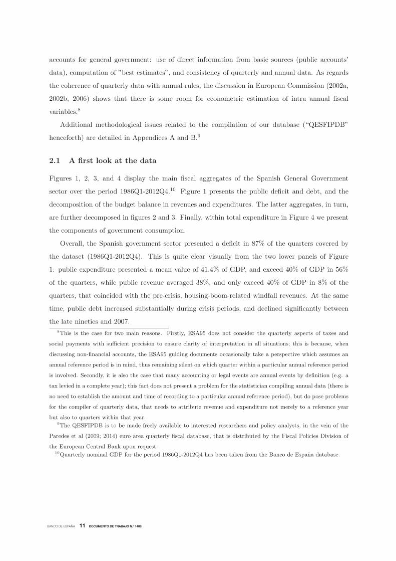
accounts for general government: use of direct information from basic sources (public accounts’
data), computation of ”best estimates”, and consistency of quarterly and annual data. As regards
the coherence of quarterly data with annual rules, the discussion in European Commission (2002a,
2002b, 2006) shows that there is some room for econometric estimation of intra annual fiscal
variables.8
Additional methodological issues related to the compilation of our database (“QESFIPDB”
henceforth) are detailed in Appendices A and B.9
2.1 A first look at the data
Figures 1, 2, 3, and 4 display the main fiscal aggregates of the Spanish General Government
sector over the period 1986Q1-2012Q4.10 Figure 1 presents the public deficit and debt, and the
decomposition of the budget balance in revenues and expenditures. The latter aggregates, in turn,
are further decomposed in figures 2 and 3. Finally, within total expenditure in Figure 4 we present
the components of government consumption.
Overall, the Spanish government sector presented a deficit in 87% of the quarters covered by
the dataset (1986Q1-2012Q4). This is quite clear visually from the two lower panels of Figure
1: public expenditure presented a mean value of 41.4% of GDP, and exceed 40% of GDP in 56%
of the quarters, while public revenue averaged 38%, and only exceed 40% of GDP in 8% of the
quarters, that coincided with the pre-crisis, housing-boom-related windfall revenues. At the same
time, public debt increased substantially during crisis periods, and declined significantly between
the late nineties and 2007.
8This is the case for two main reasons. Firstly, ESA95 does not consider the quarterly aspects of taxes and
social payments with sufficient precision to ensure clarity of interpretation in all situations; this is because, when
discussing non-financial accounts, the ESA95 guiding documents occasionally take a perspective which assumes an
annual reference period is in mind, thus remaining silent on which quarter within a particular annual reference period
is involved. Secondly, it is also the case that many accounting or legal events are annual events by definition (e.g. a
tax levied in a complete year); this fact does not present a problem for the statistician compiling annual data (there is
no need to establish the amount and time of recording to a particular annual reference period), but do pose problems
for the compiler of quarterly data, that needs to attribute revenue and expenditure not merely to a reference year
but also to quarters within that year.9The QESFIPDB is to be made freely available to interested researchers and policy analysts, in the vein of the
Paredes et al (2009; 2014) euro area quarterly fiscal database, that is distributed by the Fiscal Policies Division of
the European Central Bank upon request.10Quarterly nominal GDP for the period 1986Q1-2012Q4 has been taken from the Banco de Espana database.

BANCO DE ESPAÑA 12 DOCUMENTO DE TRABAJO N.º 1408
Figure 1: Main Government finance variables. Percent of nominal GDP.
1990 1995 2000 2005 2010
−10
−5
0
General Government deficit (−) / surplus (+)
1990 1995 2000 2005 201030
40
50
60
70
80
90General Government Debt
1990 1995 2000 2005 201030
35
40
45
50Total Government Revenues
1990 1995 2000 2005 201030
35
40
45
50Total Government Expenditure
Figure 2: General government revenues and nominal GDP (dashed line). Year-on-year growth rates
of 4-quarter-moving-sums (seasonally-adjusted, nominal terms).
1990 1995 2000 2005 2010−20
−10
0
10
20
30Total Government Revenue
1990 1995 2000 2005 2010−20
−10
0
10
20
30Direct Taxes
1990 1995 2000 2005 2010−20
−10
0
10
20
30Social Security Contributions
1990 1995 2000 2005 2010−20
−10
0
10
20
30Indirect Taxes
BANCO DE ESPAÑA 13 DOCUMENTO DE TRABAJO N.º 1408
Turning to a chronological exposition, between 1986 to 1988, following Spain’s accession to the
European Community and the commencement of a new cyclical expansion, there was a change in
direction in Spanish fiscal policy. This period was characterized by the reduction of the budget
deficit from 5.8% in 1986 to 3.3% in 1988, essentially due to the growth of government revenue.
In fact, public revenue as a percentage of GDP increased by 2.1 percentage points while public
expenditure fell by some 0.5 percentage points. Moreover, there was a significant improvement in
the primary balance, that enabled public debt to be whittled down to 39% of GDP at the end
of 1988, down from the local maximun of 43% reached in 1987Q3. Despite the reduction in the
expenditure-to-GDP ratio, public outlays registered very dynamic growth rates which prevailed for
some years, until the early nineties (see Figure 3). Such expansion is linked to the phasing-in of
the Welfare State in Spain.
This period of limited fiscal restraint came to an end in 1989, when the budget deficit started
growing again to reach 7% at the height of the economic crisis that started in 1993. The primary
balance followed a similar path to the deficit. After small surpluses between 1987 and 1989, it
moved into deficit in 1990. Finally, there was only a slight increase in public debt, to 45.6% of
GDP in 1993, primarily as a consequence of the strong growth in GDP between 1989 and 1991
(11% in nominal terms), and despite the increase in the cost of debt during this period. In the
following years however, public debt rocketed to exceed 60% of GDP in 1994, as a consequence of
the sizeable budget deficits and the fall in nominal GDP growth due to the economic crisis and the
prohibition on monetary financing of the deficit as of 1994, under the Treaty on European Union.
At the same time, the interest burden rose, reaching almost 5% of GDP in 1994.
The second half of the nineties, especially since 1996, is characterized by a protracted period of
fiscal consolidation due to the commitment to meet the convergence criteria set out in the Treaty
on European Union to regulate access to the Third Stage of EMU. Accordingly, public deficits
displayed a declining trend that spread until 2007, when an unprecedented surplus of some 2% of
GDP was recorded. Such steady and protracted reduction of general government deficits came hand
in hand with a prolonged period of economic expansion. However, not all the years between 1996
and 2007 can be duly labeled as years of “fiscal consolidation”. As Figure 1 shows, the reduction in
the public deficit was mainly the result of a drop in spending in the second half of the nineties, which
fell by more than 6 points of GDP. However, this trend of expenditure retrenchment was reverted
in the following years. In fact, public expenditure in nominal terms registered elevated growth
rates, only masked by even higher nominal GDP growth, partly due to high inflation. Moreover,

BANCO DE ESPAÑA 14 DOCUMENTO DE TRABAJO N.º 1408
Figure 3: General government expenditures and nominal GDP (dashed line). Year-on-year growth
rates of 4-quarter-moving-sums (seasonally-adjusted, nominal terms).
1990 1995 2000 2005 2010−10
0
10
20Total Government Expenditure
1990 1995 2000 2005 2010−10
0
10
20Social Payments
1990 1995 2000 2005 2010−10
0
10
20Government Gonsumption
1990 1995 2000 2005 2010
−30
−20
−10
0
10
20
Government investment
after 2004 nominal government expenditure displayed growth rates above those of nominal GDP
(Figure 3). Still, the deficit reduction continued as a result of the buoyancy of tax revenues (Figure
2), which benefited largely from the tax-friendly growth composition to a large extent linked to the
disproportionate development of the construction sector, especially related to the construction of
dwellings.
The figures also show the strong drop in revenues since the onset of the financial crisis, in
particular on indirect taxes and direct taxes, while social security contributions were more resilient.
In fact, as it is apparent from Figure 2, the most recent crisis was the only period since 1986 in
which total revenues (annualized) entered into negative territory in nominal terms. Total revenues
contracted for seven consecutive quarters, namely from 2008Q1 till 2009Q3, presenting an average
drop of 8.5% per quarter in year-on-year terms. The “double-dip” that the Spanish economy
suffered between 2011Q4 and 2013Q4 also implied some negative registers of nominal government
revenue in year-on-year terms (five consecutive quarters, from 2011Q2 to 2012Q2), even though
the tax-increasing measures enacted over that period were conductive to containing the downward
pressures arising from depressed tax bases.

BANCO DE ESPAÑA 15 DOCUMENTO DE TRABAJO N.º 1408
Figure 4: Government consumption components. Year-on-year growth rates of 4-quarters moving
sums (seasonally-adjusted, nominal terms).
1990 1995 2000 2005 2010−10
0
10
20Government Consumption
1990 1995 2000 2005 2010−10
0
10
20Compensation of public employees
1990 1995 2000 2005 2010−10
0
10
20Government employment
1990 1995 2000 2005 2010−10
0
10
20Non−wage government consumption
Looking at the most recent decade, within total public expenditure, government consumption
and investment were the most dynamic components in the pre-crisis period, and also the ones
that were contracted more in the most recent fiscal retrenchment episode, as evident from Figure 3.
Between 2008Q1 and 2010Q3 public consumption increased on average by 6% per quarter on a year-
on-year basis, though on a decreasing path, in particular since mid-2010. As of 2010Q4, government
consumption displayed negative rates of change till the end of 2012, with the exception of the first
quarter of 2011 (a quarter preceding the local and regional elections of May 2011). Within public
consumption (Figure 4) the main part of the adjustment was taken by the wage bill component,
including public employment. In turn, government investment displayed a distinctive cycle-like
pattern, typically described as being synchronized with electoral cycles. During the financial crisis,
between 2008Q1 and 2009Q4 a number of fiscal stimulus packages made public investment grow
by close to 10% in cumulative terms (6% on average per quarter in year-on-year terms), but since
2010Q1 and till 2012Q4 it dropped by almost 70%, what implied that more than 50% of the
overall expenditure adjustment done by the Spanish public administrations over the period 2010-
2012 was due to public investment reduction.11 Finally, as regards social payments, the significant
11Between 2010Q1 and 2012Q4 total expenditure fall by 2.7% of GDP. Bearing in mind that Social payments
increased by 1.3 points of GDP and interest payments by 1.2 points, the rest of components of spending fall by 5.2%

BANCO DE ESPAÑA 16 DOCUMENTO DE TRABAJO N.º 1408
increase of 2008-2009 was due to massive unemployment spending, even though the rest (including,
most notably, pensions’ spending) showed a cumulated increase of some 10%. In 2010-2012, social
payments decelerated considerably, mainly due to the cumulated fall in unemployment-related
spending, partly due to some cost-cutting measures, and the deceleration of pensions and others
(that presented a nominal increase of 5.6% between 2010Q1 and 2012Q4).
In this Section we have shown some stylized facts of fiscal policies over 1986Q1-2012Q4, that
will be complemented, from more analytical angles, in the next two Sections.
3 Cyclical properties of fiscal variables
In tables 2 and 3,we report dynamic cross-correlation functions. We look at the unconditional
correlations between detrended series at the standard business cycle frequencies. The underlying
assumption to detrending filters is that aggregate seasonally-adjusted economic time series can
be decomposed into a trend component, Tt, the so-called cyclical component, Ct, that fluctuates
around the trend, and an unpredictable random component (or irregular component), εt, i.e. yt =
Tt + Ct + εt. Most of the detrending filters take out the trend component from the original time
series, so that both the cyclical and irregular components Ct + εt are taken as a measure of the
cycle. To try to isolate the systematic autocorrelation properties of the filtered series Ct from the
irregular fluctuations or nonsystematic behavior of the series, εt, we use univariate ARIMA filters
to extract (“pre-whiten”) the later from the detrended components Ct + εt.12
Following standard practice we measure the co-movement between two series using the cross
correlation function (CCF thereafter). Each row of the table displays the CCF between a given
detrended fiscal variable at time t+k, and detrended GDP at time t.13 In selecting this statistic,
we follow the common practice in the related literature that shows results for Spain (Dolado et
al., 1993; Marın, 1997; Esteve et al., 2001; Andre and Perez, 2005; Lamo et al., 2013), and other
works in the general literature of fiscal policies’ stylized facts. Following the standard discussion in
the literature, it is said that the two variables co-move in the same direction over the cycle if the
maximum value in absolute terms of the estimated correlation coefficient of the detrended series
of GDP. Of the latter amount, government investment was responsible for 2.8 points, i.e. 53.4% of the total.12See Andre and Perez (2002; 2005) and the references quoted therein. See also den Hann (2000) for a similar
procedure in a VAR framework.13In the case of pre-whitened variables, the corresponding row of the table shows the CCF between the irregular
components of the fiscal variable fiscal variable at time t+k, and the irregular component of GDP at time t.

BANCO DE ESPAÑA 17 DOCUMENTO DE TRABAJO N.º 1408
(call it dominant correlation) is positive, that they co-move in opposite directions if it is negative,
and that they do not co-move if it is close to zero. A cut-off point of 0.20 roughly corresponds
in our sample to the value required to reject at the 5% level of significance the null hypothesis
that the population correlation coefficient is zero. Finally, the fiscal variable is said to be lagging
(leading) the real economic activity variable if the maximum correlation coefficient is reached for
negative (positive) values of k. For the sake of robustness, and following Lamo et al. (2013), we
show results for the mean of a set of standard filters14 15 as applied to seasonally-adjusted time
series. In Appendix C we describe the methods used. For ease of exposition, in Table 1 we present
the list of variables (and acronyms) used.
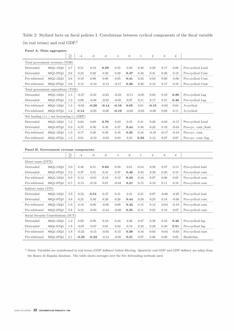
Turning to the results, Table 2, Panel 1, shows the strong and pro-cyclical behavior of total
government revenue in Spain, a result that is consistent with the evidence based on annual data for
Spain for the 1960-1990 period (see Esteve et al., 2001), and also with the existing results for the
euro area aggregate (see Paredes et al., 2009; 2014), and G7 countries (Fiorito, 1997). Total revenue
mimics the business cycle behavior in upturns and downturns, reflecting the operation of automatic
stabilizers, in a broadly contemporaneous manner – the dominant correlation is contemporaneous
when the crisis period is excluded, and when the systematic part of the correlation is cleaned up
(pre-whitened series). The dominant correlation is high, ranging between 0.5 (pre-crisis) and 0.6
(full sample). When we filter out the dynamics of the series due to systematic autocorrelation to
end up with the irregular component, the correlation is somewhat weaker but high (0.3 and 0.4,
respectively). This indicates that the unpredictable component of the series is responsible for an
important part of the pro-cyclicality of the real public revenue series. As regards relative volatility,
government revenues are much more volatile than GDP, close to three times, on average, a figure
higher than the one for the euro area. This may reflect the fact that a number of taxes, most notably
corporate taxes, property taxes and other indirect taxes, tend to follow boom-bust dynamics and
14We have selected a number of filters that are standard in the related, macroeconomic literature. The filters
are: (i) first difference filter; (ii) linear trend; (iii) Hodrick-Prescott filter for two alternative values of the band-pass
parameter: the standard 1600, and a higher value of 8000 the one suggested by Marcet and Ravn (2004) for countries
with more volatile cycles (like Spain); (iv) The Band-Pass filter of Christiano and Fitzgerald (2003), with two different
pairs of band-pass parameters [pl,pu], capturing fluctuations between 1.5 and 8 years ([pl = 6,pu=32]) and between
1.5 and 12 years ([pl = 6,pu=48]).15An alternative to the combination of filters would have been to focus on just one specific filter, for example, the
Band-Pass filter. We prefer to follow the more agnostic approach of Lamo et al. (2013) and show average results for
a number of standard filters. In any case, this is done only for the sake of exposition, and all individual filters’ results
are available from the authors upon request.

BANCO DE ESPAÑA 18 DOCUMENTO DE TRABAJO N.º 1408
Table 1: List of General Government sector variables covered, and acronyms for them.
Name of the variable Acronym Name of the variable Acronym
Net lending (+)/net borrowing (-) DEF Public debt MAL
(public surplus/deficit)
Total government revenue TOR Total expenditure TOE
Direct taxes DTX Social payments THN
Social security contributions SCT of which Unemployment benefits UNB
Total indirect taxes TIN Interest payments INT
Value Added taxes VAT Subsidies SIN
Other indirect taxes OTIN Government investment GIN
= TIN - VAT Nominal government consumption GCN
Government wage consumption expenditure COE
Non-wage final consumption expenditure OGCN
Other expenditure OTOE =
residual from TOE
Real government consumption GCR
Government employment LGN
do react to the cycle more than proportionally (Morris and Schuknecht, 2007). In addition, the
progressive structure of the income tax also causes excess volatility of income taxes relative to the
business cycle.
This is clear from Table 2, Panel 2, were we show how the standard deviation of the cyclical
component of direct taxes (mixture of household and corporate taxes) are around 5 times higher
than the one of real GDP, while that of indirect taxes is around 4 times as high, while the relative
volatility of Social Security contributions with respect to GDP ranges between 1.5 (full sample)
and 2 (pre-crisis). In this respect, it is not surprising that indirect taxes are less volatile than
direct taxes, given that, for example, tax bases such as households’ income and corporate profits
are more volatile than private sector consumption. Also, social contributions rely on personal
income, but at proportional rates and applied to censored tax bases. This creates a lower relative
volatility. In the case of Spain, the fact that unemployment benefits pay social contributions
may create some extra volatility relative to real GDP in downturns. Compared to the results of
Esteve et al. (2001) and Marın (1997), with data up the 1990s, our results by components show
robust evidence of pro-cyclicality of revenue components. In fact, when looking at the whole sample
versus the pre-crisis sample, co-movements between cyclical components are stronger in all the cases
considered. Interestingly, as regards, the leading/lagging structure of public revenue components
BANCO DE ESPAÑA 19 DOCUMENTO DE TRABAJO N.º 1408
when the whole sample is considered, the overall contemporaneous observation of Panel 1 as regards
total revenues is the combination of a leading behavior of direct and indirect taxes, while social
contributions display a lagging behavior, more consistent with the traditional role of government
revenues as automatic stabilizers.
Most existing studies look at the cyclical properties of government spending (see Frankel, Vegh
and Vuletin, 2013, and the references quoted therein). Indeed, an important reason for the usual
finding of pro-cyclical spending is precisely that government receipts get increased in booms, typ-
ically beyond expectations, and thus governments use the surplus to increase spending propor-
tionately as a consequence of political pressure or just following certain social-welfare-improving
objectives. We show the cyclical properties of total government expenditure in Table 2, Panel 1,
and those of its components in Table 3. As expected, in Table 3 total expenditure appears pro-
cyclical as well, but lagged; this behavior can be rationalized on the basis of the political economy
arguments mentioned before. The lag detected with quarterly data implies that total expenditure
follows GDP with a -minimum- delay of one year. Budgetary patterns on the spending side tend to
be quite persistent, in particular as regards sizeable items like public wages or public employment.
For example, only in the period following an economic downturn are fiscal consolidation measures
implemented, while in expansions, fresh government revenues tend to expand the public sector wage
bill with some delay. When the pre-whitened cyclical co-movements are considered, the correlation
between the shocks is barely significant.
The pro-cyclical pattern of total expenditures is due to the government consumption component
(GCR), in line with available evidence for the euro area obtained with annual data (see Lamo et
al., 2013). The pro-cyclicality of public consumption in the case of Spain is a result already
obtained in previous works for samples covering up to the beginning of the 2000s (Dolado et al.,
1993; Andre and Perez, 2005; Marın, 1997; Ortega, 1998; Esteve et al., 2001). Co-movements
among unanticipated components are also pro-cyclical and explain a significant portion of the co-
movement among cyclical components. Within government consumption (Table 4) the pro-cyclical,
lagged co-movement is explained by the wage bill, while the correlation of the cycle of real GDP
and that of non-wage government consumption is weaker, though still positive. For the whole
sample, there is a positive cyclical co-movement of public employment and real GDP, but this is
weaker that the one of the wage bill, suggesting that public wages (per employee) would be the
part of the wage bill displaying the strongest correlation. Interestingly, when the inertia of the
series is removed (pre-whitening), the cyclical correlation of public wage bill/public employment

BANCO DE ESPAÑA 20 DOCUMENTO DE TRABAJO N.º 1408
shocks/discretionary policies and real GDP shocks tend to be non-significant. At the same time,
the correlation of shocks to non-wage government consumption with real GDP shocks is negative
(counter-cyclicality). Again, these results as regards pre-whitened series might be an indication
that the components of government consumption are usually used to adjust budgetary outcomes,
with no clear pattern of individual components, while at the end the aggregate ends up being
pro-cyclical. Government investment (again in Table 3) also displays a marked pro-cyclical co-
movement. Nevertheless, when the inertia of the cycles is taken out, there remains no clear cyclical
pattern. As in the case of government consumption, this might be an indication that shocks to
government investment are used to meet budgetary outcomes, as also highlighted by Esteve et al.
(2001).
By contrast, social payments reflects a counter-cyclical pattern, mainly due to the properties
of unemployment benefits; unemployment-related spending increase in downturns and decrease
in upturns, reflecting a role of automatic stabilization. The latter evidence is consistent with
an interpretation whereby employment losses at the beginning of a cyclical downturn tend to be
associated with new unemployed receiving full-entitlement benefits (given that downturns do occur
after a good times period), coupled with the fact that the average duration of the entitlement
tends to be lower than the number of quarters the economy is below trend. In Table 4 it is
possible to see that besides the counter-cyclical pattern, unemployment spending leads the cycle,
i.e. employment destruction may start somewhat ahead of a real GDP downturn. The dominant
correlation for the whole sample is higher than the one obtained with the pre-crisis sample, given
the sizeable increase of unemployment-related spending during the most recent crisis. As regard
other social payments in cash, that include contributory and non-contributory pensions as well as
other social transfers like temporary disability, the estimated cyclical correlation is weaker than
the one estimated for unemployment benefits. Given the different nature of the components of
that aggregate, results on co-movement with the business cycle are not clear cut. In fact, while
in the pre-crisis sample a positive dominant correlation is found, consistent with the hypothesis
that social spending is increased in good times and reduced in bad times, the inclusion of the
crisis years (2008Q1-2012Q4) weakens the dominant correlation and turns it to a negative value
(counter-cyclicality). This is consistent with the observation that during the whole crisis social
payments gained weight over GDP, as they were conceived as a tool to guarantee social cohesion in
the midst of the crisis and the fiscal consolidation process that came hand-in-hand with it. In any
case, when the inertia of the series is removed, the correlation among pre-whitened series shows

BANCO DE ESPAÑA 21 DOCUMENTO DE TRABAJO N.º 1408
no particular pro- or counter-cyclical behavior, most likely reflecting the fact that decisions on
pensions are relatively erratic: in good times they are increased above determinants like inflation
or wages due to equity and/or electoral considerations, while in bad times their growth tend to be
moderated on the back of fiscal consolidation needs.
As regards the other components of spending, interest payments exhibit a counter-cyclical
behavior. In downturns interest payments increase on the back of increased public debt and,
typically in the case of Spain, rising interest rates on newly issued debt. Correlations among
shocks explain a significant portion of the cyclical co-movement. Subsidies seems to be also a
counter-cyclical policy item, even thought the correlations are relatively low. Finally, other public
expenditures, and aggregate of very different spending items given that gathers the rest of current
and capital expenditures not discussed above, displays a positive co-movement, as total expenditure,
even though it is weak.
As regards the relative volatility of real public expenditure over real GDP, as in the case of
public revenue it is higher than one, but of an order of magnitude considerably lower, being around
1.5 as compared to 3-4 in the case of total revenues. In both cases the magnitude of the relative
volatility is considerably higher that in the euro area aggregate case (see Paredes et al., 2014). This
is an issue that may deserve further attention, given the findings in the literature on the detrimental
effects of fiscal policies volatility on economic growth (Afonso and Furceri, 2010).
By component, social payments other that unemployment benefits, and government consump-
tion, are the most stable components, with relative cyclical variabilities only slightly above one,
while unemployment spending and government investment display volatilities six or more times
the volatility of real GDP. In addition, subsidies (transfers to firms), being presumably decided
on an occasional basis, are the most volatile component within the public expenditure categories
considered. The relative stability of government consumption is consistent with the fact that the
provision of public goods should be broadly independent of the business cycle. Yet, as signalled
by Fiorito (1997), government consumption does not only include such public goods as defense,
justice, etc., but also accommodates merit goods such as health or education that are partially
supplied by private units and that also involve purchases from private firms. Within government
consumption, the standard deviation of the wage component is half that of the non-wage compo-
nent, and within the wage component public employment is the only government spending item
with a relative volatility below one. The latter reflects the broad stability of most public employees
in Spain, that enjoy a per-life civil-servant status.
BANCO DE ESPAÑA 22 DOCUMENTO DE TRABAJO N.º 1408
Table 2: Stylized facts on fiscal policies I. Correlations between cyclical components of the fiscal variable
(in real terms) and real GDP.‡
Panel A. Main aggregatesσy
σx-4 -3 -2 -1 0 1 2 3 4
Total government revenues (TOR)
Detrended 86Q1-12Q4 2.7 0.51 0.53 0.59 0.55 0.58 0.48 0.29 0.17 0.06 Pro-cyclical Lead
Detrended 86Q1-07Q4 2.6 0.24 0.20 0.29 0.29 0.47 0.46 0.31 0.26 0.19 Pro-cyclical Cont.
Pre-whitened 86Q1-12Q4 3.8 0.19 0.06 0.08 0.05 0.41 0.23 0.03 0.00 -0.06 Pro-cyclical Cont.
Pre-whitened 86Q1-07Q4 3.6 0.15 -0.10 -0.13 -0.17 0.26 0.20 0.13 0.17 0.18 Pro-cyclical Cont.
Total government expenditure (TOE)
Detrended 86Q1-12Q4 1.5 -0.27 -0.31 -0.25 -0.23 -0.11 -0.05 0.04 0.19 0.36 Pro-cyclical Lag
Detrended 86Q1-07Q4 1.3 0.00 -0.08 -0.02 -0.05 0.07 0.11 0.17 0.31 0.46 Pro-cyclical Lag
Pre-whitened 86Q1-12Q4 1.4 -0.03 -0.20 -0.14 -0.16 0.05 0.01 -0.15 -0.02 0.04 A-cyclical
Pre-whitened 86Q1-07Q4 1.4 0.14 -0.05 -0.06 -0.19 -0.02 -0.03 -0.08 0.09 0.11 A-cyclical
Net lending (+) / net borrowing (-) (DEF)
Detrended 86Q1-12Q4 1.4 0.64 0.69 0.70 0.63 0.55 0.41 0.20 0.03 -0.15 Pro-cyclical Lead
Detrended 86Q1-07Q4 0.9 0.35 0.36 0.39 0.37 0.44 0.40 0.22 0.10 -0.04 Pro-cyc. cont./lead
Pre-whitened 86Q1-12Q4 1.3 0.17 0.20 0.20 0.16 0.25 0.16 -0.10 -0.17 -0.18 Pro-cyc. cont.
Pre-whitened 86Q1-07Q4 1.3 0.01 -0.10 -0.03 0.03 0.25 0.33 0.12 0.07 0.07 Pro-cyc. cont./lag.
Panel B. Government revenue components.
σy
σx-4 -3 -2 -1 0 1 2 3 4
Direct taxes (DTX)
Detrended 86Q1-12Q4 5.0 0.48 0.51 0.62 0.58 0.61 0.54 0.39 0.27 0.15 Pro-cyclical lead
Detrended 86Q1-07Q4 5.3 0.37 0.31 0.41 0.37 0.46 0.42 0.30 0.20 0.10 Pro-cyclical cont.
Pre-whitened 86Q1-12Q4 6.9 0.14 -0.01 0.19 0.12 0.33 0.18 0.07 0.06 0.05 Pro-cyclical cont.
Pre-whitened 86Q1-07Q4 6.7 0.13 -0.18 0.01 -0.04 0.21 0.15 0.10 0.11 0.16 Pro-cyclical cont.
Indirect taxes (TIN)
Detrended 86Q1-12Q4 4.3 0.52 0.54 0.47 0.41 0.41 0.21 0.07 -0.06 -0.26 Pro-cyclical lead
Detrended 86Q1-07Q4 3.8 0.25 0.30 0.26 0.28 0.44 0.30 0.25 0.18 -0.08 Pro-cyclical cont.
Pre-whitened 86Q1-12Q4 5.9 0.18 0.06 -0.06 0.09 0.42 0.15 0.12 -0.04 -0.19 Pro-cyclical cont.
Pre-whitened 86Q1-07Q4 5.8 0.13 -0.05 -0.24 -0.09 0.35 0.11 0.25 0.19 0.07 Pro-cyclical cont.
Social Security Contributions (SCT)
Detrended 86Q1-12Q4 1.4 0.03 0.08 0.18 0.24 0.36 0.37 0.38 0.42 0.46 Pro-cyclical lag.
Detrended 86Q1-07Q4 1.8 -0.07 -0.07 0.01 0.04 0.19 0.22 0.29 0.39 0.51 Pro-cyclical lag.
Pre-whitened 86Q1-12Q4 1.8 -0.22 -0.15 -0.04 0.13 0.38 0.16 0.03 -0.04 -0.03 Pro-cyclical cont.
Pre-whitened 86Q1-07Q4 2.1 -0.25 -0.22 -0.14 -0.05 0.21 0.07 0.06 0.06 0.05 Borderline
‡ Notes: Variables are transformed in real terms (GDP deflator) before filtering. Quarterly real GDP and GDP deflator are taken from
the Banco de Espana database. The table shows averages over the five detrending methods used.

BANCO DE ESPAÑA 23 DOCUMENTO DE TRABAJO N.º 1408
Table 3: Stylized facts on fiscal policies II (Main expenditure aggregates). Correlations between cyclical
components of the fiscal variable (in real terms) and real GDP.‡
σy
σx-4 -3 -2 -1 0 1 2 3 4
Social transfers other than unemployment benefits (THN - UNB)
Detrended 86Q1-12Q4 1.1 -0.35 -0.39 -0.30 -0.20 -0.12 -0.02 0.01 0.11 0.20 Count.-cyc. lead
Detrended 86Q1-07Q4 1.3 -0.06 -0.14 -0.07 0.04 0.12 0.23 0.23 0.34 0.43 Pro-cyclical lag.
Pre-whitened 86Q1-12Q4 1.7 0.00 -0.16 -0.16 -0.06 0.01 0.11 0.10 0.08 0.11 A-cyclical
Pre-whitened 86Q1-07Q4 2.0 0.08 -0.18 -0.18 -0.07 0.04 0.16 0.13 0.09 0.10 A-cyclical
Unemployment benefits (UNB)
Detrended 86Q1-12Q4 6.7 -0.52 -0.56 -0.54 -0.59 -0.47 -0.41 -0.27 -0.10 0.04 Count.-cyc. lead
Detrended 86Q1-07Q4 6.1 -0.41 -0.36 -0.28 -0.33 -0.18 -0.19 -0.12 -0.02 0.05 Count.-cyc. lead
Pre-whitened 86Q1-12Q4 6.5 0.01 -0.06 -0.14 -0.37 -0.09 -0.22 -0.16 0.04 -0.08 Count.-cyc. lead
Pre-whitened 86Q1-07Q4 6.7 -0.02 0.05 0.08 -0.14 0.05 -0.23 -0.28 -0.13 -0.17 Count.-cyc. lag.
Government consumption (GCR)
Detrended 86Q1-12Q4 1.2 -0.13 -0.05 0.14 0.20 0.31 0.25 0.26 0.26 0.37 Pro-cyclical lead
Detrended 86Q1-07Q4 1.4 -0.05 0.08 0.33 0.39 0.48 0.34 0.30 0.24 0.38 Pro-cyclical cont.
Pre-whitened 86Q1-12Q4 1.7 -0.13 -0.20 0.05 -0.03 0.30 0.05 -0.04 -0.07 0.19 Pro-cyclical cont.
Pre-whitened 86Q1-07Q4 2.0 -0.17 -0.10 0.28 0.15 0.38 0.02 -0.07 0.02 0.35 Pro-cyclical cont.
Government investment (GIN)
Detrended 86Q1-12Q4 6.6 0.13 0.18 0.23 0.25 0.26 0.25 0.28 0.30 0.38 Pro-cyclical lag.
Detrended 86Q1-07Q4 6.1 0.38 0.41 0.45 0.46 0.45 0.42 0.42 0.38 0.41 Pro-cyc. cont./lead
Pre-whitened 86Q1-12Q4 5.4 0.18 0.12 0.15 0.10 -0.03 -0.23 -0.22 -0.15 0.16 Borderline
Pre-whitened 86Q1-07Q4 6.3 0.27 0.23 0.23 0.14 0.04 -0.16 -0.13 -0.08 0.20 Pro-cyclical lead
‡ Notes: Variables are transformed in real terms (GDP deflator) before filtering. Quarterly real GDP and GDPdeflator are taken from
the Banco de Espana database. The table shows averages over the five detrending methods used.

BANCO DE ESPAÑA 24 DOCUMENTO DE TRABAJO N.º 1408
Table 4: Stylized facts on fiscal policies III (Other expenditure items). Correlations between cyclical com-
ponents of the fiscal variable (in real terms) and real GDP.‡
Panel A. Government consumption components.σy
σx-4 -3 -2 -1 0 1 2 3 4
Compensation of public employees (COE)
Detrended 86Q1-12Q4 1.6 -0.30 -0.30 -0.19 -0.09 0.07 0.15 0.23 0.31 0.43 Pro-cyclical lag.
Detrended 86Q1-07Q4 1.7 -0.11 -0.11 0.04 0.14 0.32 0.40 0.45 0.51 0.58 Pro-cyclical lag.
Pre-whitened 86Q1-12Q4 1.5 -0.16 -0.20 -0.14 -0.04 0.17 0.12 -0.02 0.12 0.12 Borderline
Pre-whitened 86Q1-07Q4 1.4 -0.15 -0.24 -0.19 -0.12 0.15 0.20 0.15 0.28 0.20 Pro-cyclical lag.
Government employment (LGN)
Detrended 86Q1-12Q4 0.8 0.19 0.20 0.24 0.26 0.28 0.27 0.26 0.29 0.27 Pro-cyclical lag.
Detrended 86Q1-07Q4 0.9 0.38 0.38 0.40 0.42 0.43 0.41 0.36 0.36 0.27 Pro-cyclical cont.
Pre-whitened 86Q1-12Q4 0.7 0.03 -0.02 -0.04 0.05 0.10 -0.04 -0.11 0.02 -0.06 A-cyclical
Pre-whitened 86Q1-07Q4 0.9 0.04 0.03 -0.01 0.09 0.13 0.00 -0.05 0.08 -0.03 A-cyclical
Non-wage government consumption (OGCN)
Detrended 86Q1-12Q4 2.5 -0.07 -0.06 0.08 0.09 0.19 0.05 0.07 0.03 0.18 Borderline
Detrended 86Q1-07Q4 3.2 -0.06 -0.03 0.16 0.16 0.24 0.01 -0.02 -0.10 0.09 Pro-cyclical cont.
Pre-whitened 86Q1-12Q4 4.5 -0.06 -0.31 -0.02 -0.07 0.23 -0.03 -0.08 -0.11 0.10 Count.-cyclical lead
Pre-whitened 86Q1-07Q4 5.2 -0.26 -0.38 0.12 0.10 0.34 0.02 -0.06 -0.05 0.19 Count.-cyclical lead
Panel B. Other government expenditure components.σy
σx-4 -3 -2 -1 0 1 2 3 4
Interest payments (INP)
Detrended 86Q1-12Q4 5.4 -0.24 -0.28 -0.33 -0.39 -0.35 -0.39 -0.33 -0.30 -0.27 Count.-cyc. lag.
Detrended 86Q1-07Q4 6.5 -0.17 -0.25 -0.34 -0.42 -0.37 -0.44 -0.35 -0.28 -0.20 Count.-cyc. lag.
Pre-whitened 86Q1-12Q4 6.3 0.02 -0.15 -0.17 -0.15 0.00 -0.18 0.07 0.14 0.12 Borderline
Pre-whitened 86Q1-07Q4 7.2 -0.04 -0.21 -0.23 -0.21 -0.03 -0.26 0.09 0.13 0.14 Count.-cyc. lag.
Subsidies (SIN)
Detrended 86Q1-12Q4 10.2 0.08 0.01 -0.05 -0.06 -0.10 0.02 0.02 0.11 0.10 A-cyclical
Detrended 86Q1-07Q4 11.9 0.05 -0.06 -0.18 -0.23 -0.31 -0.11 -0.11 0.02 -0.06 Count.-cyc. cont.
Pre-whitened 86Q1-12Q4 19.3 0.05 0.11 0.01 -0.05 -0.22 0.01 -0.05 0.02 -0.05 Count.-cyc. cont.
Pre-whitened 86Q1-07Q4 21.2 0.17 0.11 -0.06 -0.17 -0.30 0.05 0.05 0.07 -0.11 Count.-cyc. cont.
Other public expenditure (OTOE)
Detrended 86Q1-12Q4 4.7 0.20 0.20 0.24 0.24 0.22 0.23 0.19 0.17 0.20 Pro-cyc. Lead
Detrended 86Q1-07Q4 6.0 0.36 0.29 0.26 0.19 0.13 0.12 0.06 0.04 0.09 Pro-cyc. Lead
Pre-whitened 86Q1-12Q4 7.4 0.04 0.00 0.12 0.11 0.13 0.07 -0.14 -0.08 0.11 A-cyclical
Pre-whitened 86Q1-07Q4 8.9 0.26 0.13 0.10 -0.07 -0.10 -0.09 -0.18 -0.02 0.20 Pro-cyc. Lead
‡ Notes: Variables are transformed in real terms (GDP deflator) before filtering. Quarterly real GDP and GDP deflator are taken from
the Banco de Espana database. The table shows averages over the five detrending methods used.

BANCO DE ESPAÑA 25 DOCUMENTO DE TRABAJO N.º 1408
Finally, as regards government net lending, i.e. the difference between total revenues and total
expenditures, it appears clear from Table 2 that the pro-cyclical correlation has increased with the
most recent crisis, as well as its volatility. The dominant correlation ranges from 0.4 (pre-crisis) to
0.7 (full sample). In general, it can be said that government balances act as a shock absorber, but
are not more volatile that several expenditure or receipt components. The pro-cyclicality found is
in line with the results for the G7 countries of Fiorito (1997), and of Galı and Perotti (2003) for
Europe. As discussed in Lamo et al. (2013), from a theoretical point of view, our results would
render some empirical support to models that predict pro-cyclical fiscal policies. Among these are
political economy models (see the references in the introductory section, Fernandez de Cordoba et
al., 2012, and the references quoted therein) that tend to rationalize pro-cyclicality on the grounds
that bureaucrats, or governments in general, maximize the available budget for wage-related public
spending, which creates boom-bust-like dynamics as government revenue windfalls in good times
are spent in full, while fiscal consolidation needs in adverse economic circumstances force a cut in
wage and non-wage government spending. Another branch of models exploit market imperfections
to justify the existence of pro-cyclicality in fiscal policies (see, among others, Mendoza and Oviedo,
2006). Also, a classical explanation is the one of Alesina and Tabellini (2005), in which “less-
than-benevolent” governments would have incentives to appropriate rents and as such voters would
demand more public goods and fewer taxes to prevent the latter from happening when the economy
is doing well.
4 The macroeconomic impact of non-systematic fiscal policy
4.1 The existing evidence for Spain
For the case of Spain, as mentioned in the introduction, some recent papers have dealt with the mat-
ter of estimating fiscal multipliers within standard VAR frameworks. On the one hand, the papers
by de Castro (2006), de Castro and Hernandez de Cos (2008), de Castro and Fernandez-Caballero
(2013), and European Commission (2012), follow a linear SVAR approach and use similar identifi-
cation approaches. On the other hand, Hernandez de Cos and Moral-Benito (2013) move one step
forward and estimate STVAR models to compute regime-dependent fiscal multipliers. The latter
approach is in line with the traditional Keynesian view that, given slack resources in the economy,
fiscal policy may be more effective at increasing output in recessions than during normal times.
Under this hypothesis, most studies averaging the multiplier over the cycle would under-estimate
BANCO DE ESPAÑA 26 DOCUMENTO DE TRABAJO N.º 1408
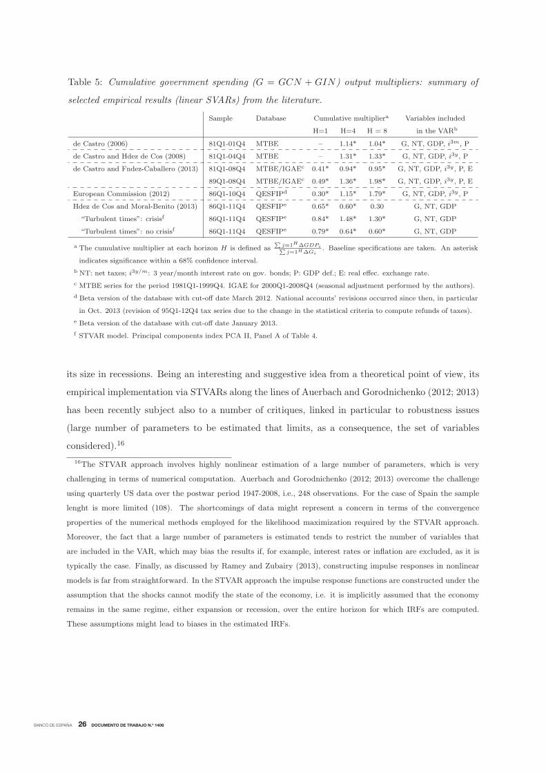
Table 5: Cumulative government spending (G = GCN + GIN) output multipliers: summary of
selected empirical results (linear SVARs) from the literature.
Sample Database Cumulative multipliera Variables included
H=1 H=4 H = 8 in the VARb
de Castro (2006) 81Q1-01Q4 MTBE – 1.14* 1.04* G, NT, GDP, i3m, P
de Castro and Hdez de Cos (2008) 81Q1-04Q4 MTBE – 1.31* 1.33* G, NT, GDP, i3y , P
de Castro and Fndez-Caballero (2013) 81Q1-08Q4 MTBE/IGAEc 0.41* 0.94* 0.95* G, NT, GDP, i3y , P, E
89Q1-08Q4 MTBE/IGAEc 0.49* 1.36* 1.98* G, NT, GDP, i3y , P, E
European Commission (2012) 86Q1-10Q4 QESFIPd 0.30* 1.15* 1.79* G, NT, GDP, i3y , P
Hdez de Cos and Moral-Benito (2013) 86Q1-11Q4 QESFIPe 0.65* 0.60* 0.30 G, NT, GDP
“Turbulent times”: crisisf 86Q1-11Q4 QESFIPe 0.84* 1.48* 1.30* G, NT, GDP
“Turbulent times”: no crisisf 86Q1-11Q4 QESFIPe 0.79* 0.64* 0.60* G, NT, GDP
a The cumulative multiplier at each horizon H is defined as∑
j=1HΔGDPi∑j=1HΔGi
. Baseline specifications are taken. An asterisk
indicates significance within a 68% confidence interval.
b NT: net taxes; i3y/m: 3 year/month interest rate on gov. bonds; P: GDP def.; E: real effec. exchange rate.
c MTBE series for the period 1981Q1-1999Q4. IGAE for 2000Q1-2008Q4 (seasonal adjustment performed by the authors).
d Beta version of the database with cut-off date March 2012. National accounts’ revisions occurred since then, in particular
in Oct. 2013 (revision of 95Q1-12Q4 tax series due to the change in the statistical criteria to compute refunds of taxes).
e Beta version of the database with cut-off date January 2013.
f STVAR model. Principal components index PCA II, Panel A of Table 4.
its size in recessions. Being an interesting and suggestive idea from a theoretical point of view, its
empirical implementation via STVARs along the lines of Auerbach and Gorodnichenko (2012; 2013)
has been recently subject also to a number of critiques, linked in particular to robustness issues
(large number of parameters to be estimated that limits, as a consequence, the set of variables
considered).16
16The STVAR approach involves highly nonlinear estimation of a large number of parameters, which is very
challenging in terms of numerical computation. Auerbach and Gorodnichenko (2012; 2013) overcome the challenge
using quarterly US data over the postwar period 1947-2008, i.e., 248 observations. For the case of Spain the sample
lenght is more limited (108). The shortcomings of data might represent a concern in terms of the convergence
properties of the numerical methods employed for the likelihood maximization required by the STVAR approach.
Moreover, the fact that a large number of parameters is estimated tends to restrict the number of variables that
are included in the VAR, which may bias the results if, for example, interest rates or inflation are excluded, as it is
typically the case. Finally, as discussed by Ramey and Zubairy (2013), constructing impulse responses in nonlinear
models is far from straightforward. In the STVAR approach the impulse response functions are constructed under the
assumption that the shocks cannot modify the state of the economy, i.e. it is implicitly assumed that the economy
remains in the same regime, either expansion or recession, over the entire horizon for which IRFs are computed.
These assumptions might lead to biases in the estimated IRFs.

BANCO DE ESPAÑA 27 DOCUMENTO DE TRABAJO N.º 1408
Fine tuning country-specific estimates is a crucial issue to draw policy lessons, given that the
most recent literature has stressed the significant heterogeneity of estimates derived from general
theoretical and empirical models (see European Commission, 2012; Favero et al., 2011). In Table
5 we summarize some selected results from the aforementioned papers as regards the impact on
real GDP of a government spending (defined as GCN + GIN) shock. Most papers look at the
pre-crisis period, and find cumulative government spending multipliers of around 1 to 1.4 after
four quarters, that increase up to 1 to 1.9 after eight quarters. Papers including post 2008Q1
figures show somewhat divergent results for linear multipliers. Results may depend, basically, on
the sample considered, the dataset, and the variables included in the empirical model, given that
identification methods are quite homogeneous across papers.
In the next subsection we update the estimates of fiscal multipliers available for Spain, in order
to deepen our understanding of a number of issues. First, we include the most recent financial
crisis episode (2008Q1-2012Q4), in order to assess its impact on estimated linear multipliers, by
comparing the full sample with the sample excluding the post 2008Q1 period. Second, we test
the sensitivity of estimated multipliers to the exclusion of relevant variables like prices and interest
rates, that tend to be mandatory in non-linear SVAR approaches, given that they are subject to “the
curse of dimensionality”. Finally, we test the sensitivity and robustness of the estimated multipliers
to alternative datasets (QESFIPDB, REMS, MTBE), to grasp some intuition on whether empirical
results may end up being influenced by that choice.
4.2 Empirical exercises
The baseline VAR includes quarterly data on public expenditure (Gt = GCN + GIN), net taxes
(NTt = TOR − THN − INP ) and GDP (yt), all in real terms,17 the GDP deflator (Pt) and the
three-year interest rate of government bonds (it). All variables are seasonally adjusted and enter in
logs except the interest rate, which enter in levels. In addition, we also add in certain specifications
the level of public debt, given that this variable has been signalled as being of relevance for the
estimation of multipliers, in particular in periods of fiscal stress (see Favero and Giavazzi, 2007).
The VARs are estimated for the period 1986Q1 to 2012Q4. The GDP volume and its deflator have
been taken from the Quarterly National Accounts (National Institute of Statistics, INE) while the
three-year bond rate has been obtained from the Banco de Espana database. The SVAR approach
in this paper is completely standard and follows as such the seminal contributions of Blanchard
17The nominal variables have been deflated by the GDP deflator in order to obtain the corresponding real values.

BANCO DE ESPAÑA 28 DOCUMENTO DE TRABAJO N.º 1408
and Perotti (2002) and Perotti (2004). For further details see Appendix D. We show the results of
our empirical exercises18 in Table 6, and figures 5 and 6.
When comparing the full sample (1986Q1-2012Q4) with the sample excluding the post 2008Q1
period, the following results are worth highlighting. First, government spending shocks’ cumulative
multipliers (panel A of Table 6 and Figure 5) are marginally higher after one and two years, but
not in the medium term. At the same time, when public debt is included in the models as an
additional variable, the responses are stronger than in the baseline case, and also the increase in
the quantitative point estimates when comparing samples. Allowing net taxes and government
spending to respond to the public debt level, in a period of fiscal stress, induces a more muted
effect on the interest rates in response to the fiscal shock. This is a channel put forward by Favero
and Giavazzi (2007) in a similar set-up to ours. Second, turning to the components of “government
spending” (panel B of Table 6, and Figure 5), the cumulated output multiplier associated to public
consumption decreases after one year when the whole sample is considered. Interestingly, this
aggregated result unveils a different behavior of output in response to the non-wage and the wage
components. On the one hand, non-wage government consumption multipliers are higher when
estimated over the whole sample. This is consistent with the presence of a higher output multiplier
in bad times, given also the direct effect on private demand of this component. On the other hand,
though, the responses of output to wage bill shocks change substantially when the 2008Q1-2012Q4
quarters are included. The channel through which government personnel expenditure affects the
economy is not only linked to the direct effect on private demand, but also to the effect through the
labor market. In this respect, after an initial positive impact in the first year (multiplier below one),
a negative and significant effect on output is observed, which can be explained by the potentially
negative effects on private investment profitability stemming from higher personnel spending by
the general government sector (Alesina et al., 2002) or by signaling effects on private sector wages
18The potential endogeneity of structural shocks may affect our results. To address this potential problem, we
test that indeed there is no co-movement between the variables included in the VAR and the estimated structural
shocks. Along the lines of Favero et al. (2011) and Auerbach and Gorodnichenko (2013), among others, we have
then regressed the structural shocks on lags of the full information set used in our VAR specification. The results
(available upon request) show that indeed the shocks are orthogonal to lags of the full information set, and mostly
orthogonal if contemporaneous information is included. Additionally, we have looked at alternative concepts of
exogeneity. Particularly, those referred as “block-exogeneity” tests which analyze, on the basis of Granger causality
tests, whether or not a variable is independent of the others (see Engle et al., 1983, for a formal description). Our
results confirm the exogeneity of the estimated structural shocks.

BANCO DE ESPAÑA 29 DOCUMENTO DE TRABAJO N.º 1408
Table 6: Cumulative output multipliers of fiscal shocks.a
Quarters
A. GOVERNMENT SPENDING SHOCK 1 4 8 12 16 20
– Sample 1986Q1 - 2012Q4
Baseline 1.23* 2.12* 2.06* 1.58* 1.15* 0.74*
Baseline: 3 variables 1.11* 1.73* 1.54* 1.17* 0.72* 0.21
Model with debt 1.34* 2.67* 2.76* 2.20* 1.68* 1.27*
– Sample 1986Q1 - 2007Q4
Baseline 1.25* 1.94* 1.87* 1.51* 1.13* 0.80*
Baseline: 3 variables 1.25* 1.84* 1.50* 1.17* 0.76* 0.31
Model with debt 1.20* 2.03* 2.14* 1.86* 1.50* 1.08*
REMS database -0.64* -0.51* -0.24 -0.56 -1.27 -2.30
MTBE database 0.51* 1.03* 1.39* 1.06* 0.64 0.20
Quarters
B. SPENDING COMPONENTS’ SHOCKS 1 4 8 12 16 20
– Sample 1986Q1 - 2012Q4
Public consumption 1.45* 2.09* 1.58* 0.52 -0.59 -1.95
– Purchases 1.64* 3.20* 3.23* 1.54 -0.75 -3.9
– Personnel expenditure 1.36* 0.73* -0.56 -2.24* -4.36* -8.07*
Public investment -0.20 0.47* 1.02* 0.84 0.01 -1.58
– Sample 1986Q1 - 2007Q4
Public consumption 1.47* 2.04* 1.87* 1.36* 0.84* 0.39
– Purchases 1.63* 2.55* 2.02* 1.15* 0.2 -0.78
– Personnel expenditure 1.52* 2.23* 2.73* 3.63* 3.81 3.60
Public investment 0.02* 0.78* 1.57* 1.58* 0.97* 0.28
Quarters
C. NET TAXES SHOCK 1 4 8 12 16 20
– Sample 1986Q1 - 2012Q4
Baseline 0.25* 0.26* 0.43* 0.59* 0.72 0.87
Baseline: 3 variables 0.26* 0.26* 0.43* 0.64* 0.84* 1.01*
– Sample 1986Q1 - 2007Q4
Baseline 0.25* 0.19* 0.71* 0.92* 1.20* 1.23*
Baseline: 3 variables 0.17* 0.02 0.15 0.21 0.29 0.3
REMS database -0.32* 0.43* 1.18* 1.33* 1.08* 0.83*
MTBE database 0.52* 0.99* 1.01* 0.64* 0.26 -0.14
a The cumulative multiplier at each horizon H is defined as∑
j=1HΔGDPi∑j=1HΔGi
. Baseline specifications
are taken. An asterisk indicates significance within a 68% confidence interval.

BANCO DE ESPAÑA 30 DOCUMENTO DE TRABAJO N.º 1408
(Lamo et al., 2012). So far, the results are in line with the flavor of those obtained in previous
papers (de Castro, 2006, de Castro and Hernandez de Cos, 2008) though much more clear-cut, in
particular as regards the evidence on the short- to medium-term output effect of the wage bill.19
Finally, it is worth mentioning that public investment shocks lead to a weaker reaction by GDP
when the 2008-2012 years are added to the sample. In fact, the sizeable investment packages
implemented to smooth the effects of the crisis in 2009-2010, mainly targeted to projects with a
limited or null impact on potential growth, were accompanied by a collapse in economic activity,
which may explain the lower multipliers. When the sample period is constrained to end in the last
quarter of 2007 public investment shocks lead to more significant GDP increases, in accordance
with previous empirical evidence for Spain.
A second issue we wanted to explore is the sensitivity of estimated multipliers to the exclusion
of relevant variables, in particular prices and interest rates, given that this is typically a must in
non-linear SVAR approaches, in order to reduce the dimensionality of the number of parameters to
be estimated. The results of a tentative exercise are presented in panel A of Table 6. In the three-
variables canonical SVAR model government spending multipliers are lower than those obtained
with five-variables, standard, SVARs. Lower multipliers arise mainly because of the feedback
effects/responses of interest rates and prices to the fiscal shock. This may help in rationalizing part
of the differences in linear SVAR estimates observed in Table 6 between the multipliers reported by
Hernandez de Cos and Moral-Benito (2013) and, for example, European Commission (2012), and
may also give an indication of potential biases in estimates obtained with non-linear models that
do exclude relevant variables.
Finally, we test the sensitivity and robustness of the estimated multipliers to alternative datasets
(QESFIPDB, REMS, MTBE) in a few cases, to grasp some intuition on whether empirical results
may end up being influenced by that choice. We restrict the comparison to the 1986Q1-2007Q4
period for which we have coverage from the three datasets at hand. First, it is worth noticing that
the government spending multipliers estimated with our dataset are significantly higher and more
persistent than those obtained with the MTBE or the REMS (in the short-term) databases (panel
A of Table 6.In addition, it seems that using REMS data always lead to less precise responses of
all variables, in view of the width of confidence bands. As regards the responses of GDP to a
shock to net taxes, they seem to be in line in the three datasets, and also similar to other studies
19In the latter respect, though, the evidence with the sample until 2007Q4 regarding shocks to the public sector
wag bill is in contrast with the aforementioned evidence for Spain.

BANCO DE ESPAÑA 31 DOCUMENTO DE TRABAJO N.º 1408
for Spain and other OECD countries, even thought the MTBE response is less persistent. GDP
rises in response to higher net taxes, with the exception of the contemporaneous reaction in the
REMS case. Admittedly, the increase is at odds with almost any theoretical model. This pattern is
observed in the short term by Perotti (2004), de Castro and Hernandez de Cos (2008) or Heppke-
Falk et al. (2006), among others, which probably reveals the difficulty to identify net tax shocks
properly. In all cases, government spending declines and recovers later on, standing significantly
above the baseline in the medium term. This positive reaction of expenditure seems in line with
the tax-and-spend view of fiscal policy.20
5 Conclusions
In this paper we provide a comprehensive database of quarterly fiscal variables suitable for macroe-
conomic analysis built up on the basis of state-of-the-art macroeconometric models. All models are
multivariate, state space mixed-frequencies models, estimated with available national accounts fis-
cal data (mostly annual) and, more importantly, monthly and quarterly information taken from all
available sources of fiscal data. The database spans over the period 1986Q1-2012Q4, and covers a
wide number of fiscal aggregates, suitable for macroeconomic analysis. All the time series included
are presented in gross (non-seasonally adjusted) and seasonally adjusted terms. We focus solely
on intra-annual fiscal information for interpolation purposes. This approach allows us to capture
genuine intra-annual ”fiscal” dynamics in the data, so that we avoid two important problems that
are present in fiscal time series interpolated on the basis of general macroeconomic indicators: (i)
the endogenous bias that arises if the so interpolated fiscal series were used with macroeconomic
variables to assess the impact of fiscal policies; (ii) the well-known decoupling of tax collection from
the evolution of macroeconomic tax bases (revenue windfalls/shortfalls). On the basis of our quar-
terly fiscal database we provide in the paper a number of applications that highlight its usefulness
for macroeconomic analysis and policy.
Firstly, we provide some stylized facts on the cyclical properties of fiscal policies. We find that
total revenues in Spain display a pro-cyclical behavior, that can be to a large extent explained by
discretionary changes in policy (unpredictable component), and are much more volatile than GDP,
most likely due to the fact that a number of taxes, most notably corporate taxes, property taxes
and other indirect taxes, tend to follow boom-bust dynamics, and also to the progressive structure
20de Castro et al. (2004) provide some evidence supporting this view for Spain.

BANCO DE ESPAÑA 32 DOCUMENTO DE TRABAJO N.º 1408
Figure 5: Response to government spending shocks: government consumption (GCN) and invest-
ment (GIN) aggregate, government consumption – including components: COE and OGCN – and
government investment. Baseline sample: 1986Q1-2012Q4.

BANCO DE ESPAÑA 33 DOCUMENTO DE TRABAJO N.º 1408
Figure 6: Response to government spending shocks, alternative databases.

BANCO DE ESPAÑA 34 DOCUMENTO DE TRABAJO N.º 1408
of the income tax. Some studies have hinted at pro-cyclical revenues as a source of pro-cyclical
government spending. In fact, we find that total expenditure appears pro-cyclical as well, but
lagged. The pro-cyclical pattern of total expenditures is due to the government consumption and
investment components. Social transfers, particularly unemployment-related expenditure, on the
contrary, present a distinct counter-cyclical behavior. Public spending, overall, is found to be more
volatile that real GDP, and higher than comparable euro area reference variables.
Secondly, we run standard SVAR models and provide some updated estimates and insights on
the impact of changes in fiscal aggregates on macroeconomic variables. First, when including the
most recent financial crisis episode (2008Q1-2012Q4), government spending shocks are marginally
higher, in particular when taxes and spending are allowed to respond to public debt. As regards
components, the negative medium-term effect of wage bill shocks gets clearly profiled, compared
to less clear-cut results in other studies, while at the same time the positive impact of non-wage
government shocks increased with the crisis. Second, we show that estimated multipliers may be
sensitive to the exclusion of relevant variables like prices and interest rates, and as a consequence
results from models more computationally-intensive models that are force to drop relevant variables,
would have to be read from this perspective. Finally, we test the sensitivity and robustness of the
estimated multipliers to alternative datasets (QESFIPDB, REMS, MTBE): it seems that the choice
of the dataset might not be neutral. As regards the latter, thus, we feel reassured with our approach
of trying to advance the frontier of data availability for the profession, by improving in a transparent
way the methodology and inputs used to overcome the limitations of available official statistics to
carry out studies on the macroeconomic impact of fiscal policies.

BANCO DE ESPAÑA 35 DOCUMENTO DE TRABAJO N.º 1408
haviour of government expenditures in developing countries”, NBER Working Papers 15119.
Alesina, A., S. Ardagna, R. Perotti, and F. Schiantarelli (2002), “Fiscal policy, profits and invest-
ment”, American Economic review, 92, pp. 571-589.
Alesina, A., Campante, F., and Tabellini, G. (2008): Why is fiscal policy often procyclical?,
Journal of the European Economic Association 6, pp. 1006-1036.
Alesina, A. and G. Tabelline (2005), “Why is Fiscal Policy Often Procyclical?”, NBER Working
Paper No. 11600.
Andre, F.J. and J. J. Perez (2005), “Robust stylized facts on comovement for the Spanish econ-
omy”, Applied Economics, 37, pp. 453-462.
Auerbach A. J. and Gorodnichenko, Y. (2012) “Measuring the output responses to fiscal policy,”
American Economic Journal: Economic Policy, 4, 127.
Auerbach, A. and Gorodnichenko, Y. (2013) “Fiscal Multipliers in Recession and Expansion”, in
A. Alesina and F. Giavazzi, eds., “Fiscal Policy after the Financial Crisis”. The University
of Chicago Press.
Blanchard, O. J. and R. Perotti (2002), “An Empirical Characterization of the Dynamic Effects of
Changes in Government Spending and Taxes on Output”, Quarterly Journal of Economics,
117, pp. 1329-1368.
Borjas, G. J. (1984): “Electoral cycles and the earnings of Federal bureaucrats”, Economic Inquiry
22, pp. 447-459.
References
Afonso, A. and D. Furceri (2010), “Government size, composition, volatility and economic growth”,
European journal of Political Economy 26, pp. 517-532.
Afonso, A., L. Agnello,and D. Furceri (2010), “Fiscal policy responsiveness, persistence, and
discretion”, Public Choice 145, pp. 503-530.
Aghion P., D. Hemous, and E. Kharroubi (2009), “Credit Constraints, Cyclical Fiscal Policy and
Industry Growth”, NBER Working Paper 15119.
Akitoby, B., B. J. Clements, S. Gupta, and G. Inchauste (2004), “The cyclical and long-term be-

BANCO DE ESPAÑA 36 DOCUMENTO DE TRABAJO N.º 1408
Bouthevillain, C., J. Caruana, C. Checherita, J. Cunha, E. Gordo, S. Haroutunian, A. Hubic, G.
Langenus, B. Manzke, J. J. Perez and P. Tommasino (2009), “Pros and cons of various fiscal
measures to stimulate the economy”, Central Bank of Luxembourg Working Paper, 40.
Christiano, L. J. and T. J. Fitzgerald (2003), “The Band Pass Filter”, International Economic
Review 44, pp. 435-465.
Corrales, A. y D. Taguas (1991), “Series macroeconomicas para el periodo 1954-88: un intento de
homogeneizacion”, en Molinas, C. et al. (eds.), La economıa espanola, una perspectiva
macroeconomica, Instituto de Estudios Fiscales.
Coricelli, F. and R. Fiorito (2013), “Myths and fact about fiscal discretion: a new measure of dis-
cretionary expenditure”, Documents de Travaildu Centre d’Economie de la Sorbonne 13033,
Universite Pantheon-Sorbonne (Paris 1), Centre d’Economie de la Sorbnne.
de Castro, F. (2006), “The macroeconomic effects of fiscal policy in Spain”, Applied Economics,
38, pp. 913-924.
de Castro, F., Gonzalez-Paramo, J.M., Hernandez de Cos, P. (2004), “Fiscal consolidation in
Spain: Dynamic interdependence of public spending and revenues”, Investigaciones Economicas
XXXVIII, pp. 193-207.
de Castro, F and P. Hernandez de Cos (2008), “The economic effects of fiscal policy: the case of
Spain”, Journal of Macroeconomics, 30, pp. 1005-1028.
de Castro, F and L. Fernandez-Caballero (2013), “The Effects of Fiscal Shocks on the Exchange
Rate in Spain”, The Economic and Social Review, 44, pp. 151-180.
Bosca, J. E., A. Dıaz, R. Domenech, J. Ferri, E. Perez, and L. Puch (2011), “A rational expec-
tations model for simulation and policy evaluation of the Spanish economy”, SERIEs 1, pp.
135-169.
Bosca, J. E., A. Bustos, A. Dıaz, R. Domenech, J. Ferri, E. Perez, and L. Puch (2007), “The
REMSDB Macroeconomic Database of the Spanish Economy”, Instituto de Economıa Inter-
nacional WP0704, , Universitat de Valencia.
Boussard, J., F. de Castro, M. Salto (2012), “Fiscal Multipliers and Public Debt Dynamics in
Consolidations”, European Economy, Economic Papers 460, European Commission, July.
BANCO DE ESPAÑA 37 DOCUMENTO DE TRABAJO N.º 1408
Esteve, V., J. Sapena, J. and C. Tamarit (2001), “Propiedades cıclicas y cambios estructurales en
los series fiscales macroeconomicas de la economıa espanola, Hacienda Publica Espanola, 157,
pp. 9-44.
Estrada, A., J.L. Fernandez, E. Moral,and A.V. Regil (2004), “A quarterly macroeconometric
model of the Spanish economy”, Banco de Espana Working Paper No. 0413.
European Commission (2002a), Reg. (EC) No 1221/2002 of the European Parliament and of the
Council of 10 June 2002 on quarterly non-financial accounts for general government.
European Commission (2002b), ESA95 manual on government deficit and debt, Methods and
Nomenclatures series, European Commission, Luxembourg.
European Commission (2006), Manual on quarterly non-financial accounts for general government,
European Commission, Luxembourg.
European Commission (2007). Quarterly government accounts and fiscal surveillance, pp 103-106
in Public Finances in EMU, European Commission, Brussels.
European Commission (2012), “Review of existing estimates of fiscal multipliers”, Chapter 2 (pp.
119-162) in Part III of “Public Finances in EMU - 2012”, European Economy 4/2012
Favero, C. and F. Giavazzi (2007), “Debt and the effects of fiscal policy”, NBER Working Papers
12822.
Favero, C., Giavazzi, F., and Perego, J. (2011), “Country Heterogeneity and the International
Evidence on the Effects of Fiscal Policy”, IMF Economic Review, 59, pp. 652-682.
den Haan, W. (2000), “The comovement between output and prices”, Journal of Monetary Eco-
nomics 46, pp. 3-30.
Dilnot, A. (2012), ”Numbers and Public Policy: The Power of Official Statistics and Statistical
Communication in Public Policymaking”, Fiscal Studies 33, pp. 429-448.
Dolado, J., M. Sebastian, and J. Valles (1993), “Cyclical patterns of the Spanish economy”,
Investigaciones Economicas, 17, pp. 445-73.
Engle, R., Hendry, D.F. and Richard, J.F. (1983), “Exogeneity”, Econometrica, 51, pp. 277-304.

BANCO DE ESPAÑA 38 DOCUMENTO DE TRABAJO N.º 1408
Galı, J. and R. Perotti (2003), “Fiscal Policy and Monetary Integration in Europe”, Economic
Policy, 18, pp. 533-572.
Gomez, V. and A. Maravall (1996), “Programs TRAMO (Time series Regression with Arima noise,
Missing observations, and Outliers) and SEATS (Signal Extraction in Arima Time Series).
Instructions for the User”, Banco de Espana Working Paper No. 9628.
Harvey, A. (1989), Forecasting Structural Time Series Models and the Kalman Filter. Cambridge
University Press. UK.
Harvey, A. and Chung, C. (2000), “Estimating the underlying change in unemployment in the
UK”, Journal of the Royal Statistical Society, Series A, 163, pp. 303-339.
Heppke-Falk, K.H., J. Tenhofen and G.B. Wolff (2006), “The macroeconomic effects of exogenous
fiscal policy shocks in Germany: a disaggregated SVAR analysis”. Deutsche Bundesbank.
Discussion Paper Series 1: Economic Studies No 41/2006.
Hernandez de Cos, P. and Moral Benito, E. (2013), “Fiscal Multipliers in Turbulent Times: the
Case of Spain”, Banco de Espana Working Paper No. 1309.
Lamo, A., Perez, J. J. and Schuknecht, L. (2012), “Public or Private Sector Wage Leadership?
An International Perspective”, The Scandinavian Journal of Economics, 114, pp. 228-244.
Lamo, A., Perez, J.J. and Schuknecht (2013), “The cyclicality of consumption, wages and employ-
ment of the public sector in the euro area”, Applied Economics, 45, pp. 1551-1569.
Lane, P. (2003): “The cyclical behaviour of fiscal policy: evidence from the OECD”, Journal of
Public Economics, 87, pp. 2661-2675.
Fernandez-Caballero, L., D. J. Pedregal, D.J., and J. J. Perez (2012), “Monitoring sub-central
government spending in Spain”, Hacienda Publica Espanola, 202, pp. 77-104.
Fernandez de Cordoba, G., J. J. Perez and J. L. Torres (2012), “Public and private sector wages
interactions in a general equilibrium model”, Public Choice, 150, pp. 309-326.
Fiorito, R. (1997), “Stylized facts on government finance in the G-7”, IMF Working Paper
WP/97/141.
Frankel, J. A., C. Vegh, and G. Vuletin (2013), “On graduation from fiscal procyclicality”, Journal
of Development Economics, 100, pp. 32-47.
BANCO DE ESPAÑA 39 DOCUMENTO DE TRABAJO N.º 1408
Mendoza, E. G. and P. M. Oviedo (2006): “Fiscal policy and macroeconomic uncertainty in
developing countries: The tale of the tormented insurer”, NBER Working Paper No 12586.
Moauro F. and Savio G. (2005), “Temporal Disaggregation Using Multivariate Structural Time
Series Models”, Econometrics Journal, 8, pp. 214-234.
Morris, R. and L. Schuknecht (2007), “Structural balances and revenue windfalls - the role of asset
prices revisited”, ECB Working Paper No 737.
Morris, R., C.R. Braz, F. de Castro, S. Jonk, J. Kremer, S. Linehan, M.R. Marino, C. Schalck
and O. Tkacevs (2009), “Explaining government revenue windfalls and shortfalls: an analysis
for selected EU countries”, European Central Bank, working paper 1114, November.
Ortega, E. (1998), “The Spanish business cycle and its relationship to Europe”. Banco de Espana
Working Paper No 9819.
Paredes, J., D.J. Pedregal, and J. J. Perez (2009), “A quarterly fiscal database for the euro area
based on intra-annual fiscal information”. Banco de Espana Working Paper, No. 0935.
Paredes, J., D.J. Pedregal, and J. J. Perez (2014),“Fiscal policies in the euro area: expanding the
toolkit”, mimeo, European Central Bank.
Pedregal, D. J. and J. J. Perez (2010), “Should quarterly government finance statistics be used
for fiscal surveillance in Europe?”, International Journal of Forecasting 26, pp. 794–807.
Perotti, R. (2004), “Estimating the effects of fiscal policy in OECD countries”. Proceedings,
Federal Reserve Bank of San Francisco.
Proietti T. and F. Moauro (2006), “Dynamic factor analysis with non-linear temporal aggregation
constraints”. Journal of the Royal Statistical Society Series C, Royal Statistical Society, 55,
pp. 281-300.
Lane, P. and Tornell, A. (1996): Power, growth, and the voracity effect, Journal of Economic
Growth, 1, 213-241.
Marcet, A. and M. Ravn (2004), “The HP-filter in cross-country comparisons”, CEPR Discussion
Paper 4244.
Marın, J. (1997), “Efectos estabilizadores de la polıtica fiscal”. Estudios Economicos, 58, Servicio
de Estudios, Banco de Espana.

BANCO DE ESPAÑA 40 DOCUMENTO DE TRABAJO N.º 1408
Strawczynski, M. and J. Zeira (2009), “Cyclicality of Fiscal Policy: Permanent and Transitory
Shocks”, CEPR Discussion Papers 7271.
Wren-Lewis, S. (2013), “Annoying Anti-Fiscal Stimulus arguments”, July post at Economist’s
View.
Ramey, V., and S. Zubairy (2013), “Government Spending Multipliers in Good Times and in Bad:
Evidence from U.S. Historical Data”, mimeo.
Spilimbergo, A., S. Symansky, O. Blanchard and A. Cottarelli (2008): “Fiscal policy for the crisis”.
IMF Position Note. Washington: SPN/08/01.

BANCO DE ESPAÑA 41 DOCUMENTO DE TRABAJO N.º 1408
A Main elements of the quarterly fiscal database
Data inputs. The variables of interest are quarterly general government accounts on an ESA95
basis. Quarterly, non seasonally adjusted figures are available from 2000 onwards, as mentioned
above. Annual ESA95 data fully consistent with the quarterly figures start in 1995. Nevertheless,
annual ESA79 figures are available from 1985 to 1998. Therefore, we extended our annual ESA95
dataset backwards by means of the annual growth rates of ESA79 figures. The corresponding
annual values are used as an anchor for the quarterly interpolation procedure. As regards short-
term indicators, we use national accounts and cash data for different revenue and expenditure items
available for the different sub-sectors and public entities, at quarterly and monthly frequencies as
indicators to interpolate the quarterly ESA95 missing values. Quarterly and monthly fiscal variables
(indicators) are also taken from the IGAE and the Ministry of Employment (State Secretary of the
Social Security). For the Central government and the Social Security subsectors, short-term public
finance statistics in Spain are published timely, with a broad coverage of budgetary categories.
For the former, monthly figures in ESA95 (NA) standards covering all the relevant revenue and
expenditure details are published within one month while for the latter monthly cash figures are
made available with a short delay and cover both the Social Security System and the Public
Employment System. We also use some derived indicators of regional governments’ spending. On
available data for the sub-national governments and the developments of indicators suitable for
short-term forecasting in Spain, see Fernandez-Caballero, Pedregal and Perez (2012).
Empirical methodology. The basic model is of the Unobserved Component Model class known
as the Basic Structural Model (Harvey, 1989), that decomposes a set of time series in unobserved
though meaningful components from an economic point of view (mainly trend, seasonal and irregu-
lar). Given that the data used are sampled at different frequencies (annual, quarterly and monthly)
we use a mixed-frequencies formulation, along the lines of Harvey and Chung (2000), Moauro and
Savio (2005), and Proietti and Moauro (2006). The modeling approach is described in detail in
Appendix B.
Output database. The list of variables’ names is shown in Table 1. We provide a quite disaggre-
gated set of nominal fiscal variables for the General Government sector in ESA95 terms, seasonally

BANCO DE ESPAÑA 42 DOCUMENTO DE TRABAJO N.º 1408
rope is an important one, as signalled in European Commission (2007).21 On the revenue side of
government accounts the database covers total government revenue, direct taxes (with a proxy for
the breakdown between direct taxes paid by households and firms), social security contributions
(with a proxy for the breakdown between contributions paid by employers and others), and to-
tal indirect taxes. On the expenditure side, it covers total expenditure, social payments (of which
also unemployment benefits), interest payments, subsidies, government investment and government
consumption. Given the relevance of the latter variable (part of the demand side of GDP), we pro-
vide the breakdown between nominal and real government consumption, the breakdown between
government wage and non-wage consumption expenditure, and government employment. The net
lending of the government, a key policy variable, can be computed as the difference between total
revenues and total expenditures. We also provide quarterly public debt for the period of reference.
B Methodology to compute the quarterly fiscal database
The exposition in this section follows closely Pedregal and Perez (2010). The starting point of the
modeling approach is to consider a multivariate Unobserved Components Model known as the Basic
Structural Model (Harvey, 1989). A given time series is decomposed into unobserved components
which are meaningful from an economic point of view (trend, Tt, seasonal, St, and irregular, et).
Equation (B1) displays a general form, where t is a time sub-index measured in quarters, zt denotes
the variable in ESA95 terms expressed at an annual and quarterly sampling interval (depending on
availability) for our objective time series, and ut represents the vector of quarterly indicators.
⎡⎣ zt
ut
⎤⎦ = Tt + St + et (B1)
The general consensus in this type of multivariate models in order to enable identifiability is to
build SUTSE models (Seemingly Unrelated Structural Time Series). This means that components
of the same type interact among them for different time series, but are independent of any of
the components of different types. In addition, statistical relations are only allowed through the
covariance structure of the vector noises, but never through the system matrices directly. This
21The type of models that we use encompass the estimation of seasonal components, and so it is possible to re-
cover model-consistent seasonally-adjusted series. Nevertheless, the companion database we provide in Excel format
includes seasonally-adjusted series based on the well-known program TRAMO-SEATS (Gomez and Maravall, 1996),
given that this is the standard method used by many National Statistical Institutes to seasonally-adjust macroeco-
nomic time series.
and non-seasonally adjusted. The issue of seasonal adjustment of quarterly fiscal variables in Eu-
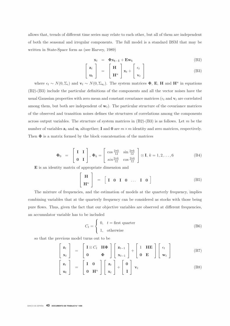
BANCO DE ESPAÑA 43 DOCUMENTO DE TRABAJO N.º 1408
allows that, trends of different time series may relate to each other, but all of them are independent
of both the seasonal and irregular components. The full model is a standard BSM that may be
written in State-Space form as (see Harvey, 1989)
xt = Φxt−1 +Ewt (B2)⎡⎣ zt
ut
⎤⎦ =
⎡⎣ H
Hu
⎤⎦xt +
⎡⎣ εt
vt
⎤⎦ (B3)
where εt ∼ N(0,Σε) and vt ∼ N(0,Σvt). The system matrices Φ, E, H and Hu in equations
(B2)-(B3) include the particular definitions of the components and all the vector noises have the
usual Gaussian properties with zero mean and constant covariance matrices (εt and vt are correlated
among them, but both are independent of wt). The particular structure of the covariance matrices
of the observed and transition noises defines the structures of correlations among the components
across output variables. The structure of system matrices in (B2)-(B3) is as follows. Let m be the
number of variables zt and ut altogether; I and 0 are m×m identity and zero matrices, respectively.
Then Φ is a matrix formed by the block concatenation of the matrices
Φ0 =
⎡⎣ I I
0 I
⎤⎦ , Φk =
⎡⎣ cos 2πk
12 sin 2πk12
sin2πk12 cos 2πk
12
⎤⎦⊗ I, k = 1, 2, . . . , 6 (B4)
E is an identity matrix of appropriate dimension and⎡⎣ H
Hu
⎤⎦ =
[I 0 I 0 . . . I 0
](B5)
The mixture of frequencies, and the estimation of models at the quarterly frequency, implies
combining variables that at the quarterly frequency can be considered as stocks with those being
pure flows. Thus, given the fact that our objective variables are observed at different frequencies,
an accumulator variable has to be included
Ct =
⎧⎨⎩
0, t = first quarter
1, otherwise(B6)
so that the previous model turns out to be⎡⎣ zt
xt
⎤⎦ =
⎡⎣ I⊗ Ct HΦ
0 Φ
⎤⎦⎡⎣ zt−1
xt−1
⎤⎦+
⎡⎣ 1 HE
0 E
⎤⎦⎡⎣ εt
wt
⎤⎦ (B7)
⎡⎣ zt
ut
⎤⎦ =
⎡⎣ I 0
0 Hu
⎤⎦⎡⎣ zt
xt
⎤⎦+
⎡⎣ 0
I
⎤⎦ vt (B8)

BANCO DE ESPAÑA 44 DOCUMENTO DE TRABAJO N.º 1408
Given the structure of the system and the information available, the Kalman Filter and Fixed
Interval Smoother algorithms provide an optimal estimation of states. Maximum likelihood in the
time domain provides optimal estimates of the unknown system matrices, which in the present
context are just covariance matrices of all the vector noises involved in the model. The use of
the models selected and the estimation procedures described in the previous paragraph, allows
the estimation of models with unbalanced data sets, i.e. input variables with different sample
lengths. This is a feature of relevance for the construction of the database at hand, given occasional
differences in temporal coverage of indicators.
In our case, particular empirical specifications for each variable will be considered in the light
of the available information (fiscal indicators). For instance, for the case of total government
revenues, z comprises total government revenues in National Accounts terms, a variable that is
available at the annual frequency from 1986-1999 and at the quarterly frequency from 2000Q1-
2010Q4, while u is a matrix composed of three series (available at the quarterly frequency for the
whole sample period): (i) a proxy to general government total revenues in public accounts (cash)
terms; (ii) Central government total revenues and (iii) Social Security (SSS+SPEE) sector’s total
revenues. In order to reduce the dimensionality of our models and somewhat avoid the “curse of
dimensionality” we opted for variable-by-variable models. By this we mean that, in all cases,z
encompasses just one time series (annual/quarterly), and u the set of indicators corresponding to
the latter variable, with a maximum of five indicators.
C Description of detrending methods
We consider a quite standard set of detrending methods:
• First order differencing takes the cycle to be the variable in first differences. Thus it assumes
that the trend is the lagged variable, or similarly the series is a random walk with no drift.
Therefore yt can be represented as: yt = yt−1 + Ct + εt where the trend is Tt = yt−1 and an
estimate of the detrended component is obtained as yt − yt−1.
• An alternative method of detrending is by removing a deterministic trend; the usual procedure
is to take the least squares residual after regressing the series on a constant and a polynomial
function of time. The implicit assumption is that the trend and cyclical components are
orthogonal, and that Tt is a deterministic process which can be approximated with polynomial
BANCO DE ESPAÑA 45 DOCUMENTO DE TRABAJO N.º 1408
functions of time. These assumptions imply a model for yt of the form: yt = Tt + Ct + εt,
Tt = f(t), and we take f(t) = a0 + a1 t+ a2 t2. Even though the disturbance may be serially
correlated, it can be shown that the unknown parameters in f(t) can be estimated efficiently
by ordinary least squares.
• The Hodrick and Prescott filter (HP Filter) extracts a stochastic trend that moves smoothly
over time and is not correlated with the cycle component. The HP filter depends on a
smoothing parameter (λ) that penalizes large fluctuations. A large λ implies a higher penalty
and, therefore, a smoother cycle.
• The band pass filter is a frequency domain based filter. It assumes that the trend component
has the power at lower frequencies of the spectrum. The choice in this procedure is to define
the limits of the frequency band, say pl and pu, to isolate the cyclical component with a
period of oscillation between pl and pu. We use an “optimal” finite sample approximation for
the band pass filter as proposed by Christiano and Fitzgerald (2003). We make two choices
for the cycle length between 1.5 and 8 years, [pl, pu] = [6, 48], and between 1.5 and 6 years,
[pl, pu] = [6, 32], removing thus all the fluctuations that have a periodicity larger than 8(6) or
smaller than 1.5 years.
• As regards the procedure to isolate the pure irregular component of the time series of interest,
we follow the traditional approach of pre-whitening the series of interest, by means of ARIMA
specifications, as in Andre and Perez (2002; 2005). Let’s assume a given cyclical component
Ct is representable by a linear model of the general ARIMA class φ(B)Ct = θ(B)εt where
εt is a white noise variable, and φ(B), θ(B) are polynomials in the lag operator B. Pre-
multiplying Ct by an estimate of θ(B)−1φ(B) provides a pre-whitened version of Ct, which is
an estimate for εt, a white noise variable representing the purely stochastic component of Ct.
If the series yt follows the above mentioned ARIMA process, the dynamic properties of the
detrended series, call it yFt can be studied by means of expression yFt = F (B)yt = F (B) θ(B)φ(B)εt
= Π(B)εt, where F(B) is the filter applied to detrend the series. Thus, obtaining an estimate
Π(B) of Π(B) it is possible to generate the pre-whitened series εt =Π−1(B)yFt . If properly
applied this method should be independent of the filtering procedure as correlations would
be computed among irregular components.

BANCO DE ESPAÑA 46 DOCUMENTO DE TRABAJO N.º 1408
D The SVAR approach
The reduced-form baseline VAR is specified in levels. Xt ≡ (gt, tt, yt, pt, rt) is the vector of en-
dogenous variables and D(L) is an autoregressive lag-polynomial. The benchmark specification
includes a constant and a deterministic time trend. The vector Ut ≡ (ugt , utt, u
yt , u
pt , u
rt ) contains
the reduced-form residuals, which in general will present non-zero cross-correlations. The baseline
VAR includes four lags of each endogenous variable according to the information provided by LR
tests, the Akaike information criterion and the final prediction error.
We apply the identification strategy proposed by Blanchard and Perotti (2002) and Perotti
(2004), which exploits decision lags in policy making and information about the elasticity of fiscal
variables to economic activity. Their strategy relies on the assumption that the reduced-form
residuals of the gt and tt equations, ugt and utt, can be thought of as linear combinations of three
types of shocks: a) the automatic responses of spending and net taxes to the rest of macroeconomic
variables in the system, b) systematic discretionary responses of fiscal policy to the same set of
macro variables and c) random discretionary fiscal policy shocks, which are the truly uncorrelated
structural fiscal policy shocks whose effects are the purpose of our analysis.
The innovations model can be written as ΓUt = BVt, where Vt ≡ (egt , ett, e
yt , e
pt , e
rt ) is the vector
containing the orthogonal structural shocks. Accordingly, the reduced-form residuals are linear
combinations of the orthogonal structural shocks of the form Ut = Γ−1BVt. The respective matrices
Γ and B can be written as:
Γ =
⎛⎜⎜⎜⎜⎜⎜⎜⎜⎜⎝
1 0 −αg,y −αg,p −αg,r
0 1 −αt,y −αt,p −αt,r
−γy,g −γy,t 1 0 0
−γp,g −γp,t −γp,y 1 0
−γr,g −γr,t −γr,y −γr,p 1
⎞⎟⎟⎟⎟⎟⎟⎟⎟⎟⎠
and
B =
⎛⎜⎜⎜⎜⎜⎜⎜⎜⎜⎝
1 βg,t 0 0 0
βt,g 1 0 0 0
0 0 1 0 0
0 0 0 1 0
0 0 0 0 1
⎞⎟⎟⎟⎟⎟⎟⎟⎟⎟⎠

BANCO DE ESPAÑA 47 DOCUMENTO DE TRABAJO N.º 1408
approving and implementing new measures in response to specific economic circumstances typically
takes longer than three months. Hence, one key assumption in this approach is that quarterly
variables allow setting discretionary contemporaneous responses of fiscal variables to changes in
underlying macroeconomic conditions to zero. Therefore, the coefficients αi,j ’s only reflect the
automatic responses of fiscal variables to the rest of the variables of the system, the first source of
innovations aforementioned.
The way fiscal variables are defined allows making further assumptions concerning the values
of the αi,j ’s. Specifically, the semi-elasticities of fiscal variables to interest rate innovations are
set to zero given that interest payments on government debt are excluded from both definitions.
Moreover, the automatic responses of public expenditure to economic activity and the real exchange
rate are also set to zero. The case of the price elasticity is different because some share of purchases
of goods and services is likely to respond to the price level. Thus, we set the price elasticity of
government expenditure to -0.5.
Output and price elasticities of net taxes, αt,y and αt,p, are estimated at 0.64 and 0.87, re-
spectively, fully in line with those in de Castro and Hernandez de Cos (2008). These are obtained
as weighted averages of the elasticities of the different net-tax components, including transfers,
computed on the basis of information like statutory tax rates and estimations of the contempora-
neous responses of the different tax-bases and, in the case of transfers, the relevant macroeconomic
aggregate to GDP and price changes.
Furthermore, given that our main interest lies on expenditure shocks we assume that spending
decisions are prior to tax ones, which implies a zero value for βg,t. This allows us to retrieve
egt directly and use it to estimate βt,g by OLS, which completes the identification of the first
two equations. For the remaining shocks the sequential ordering uyt , upt and urt is imposed. The
corresponding structural shocks are estimated by instrumental variables in turn, using egt and ett
as instruments for ugt and utt, respectively. In any case, since we are interested in studying the
effects of fiscal policy shocks, the ordering for the remaining variables is immaterial to the results.
Impulse response functions are reported jointly with 68 % confidence bands obtained by Monte
Carlo integration methods with 1000 replications.
As we are interested in analysing the effects of ”structural” discretionary spending shocks egt on
the rest of the variables of the system, estimations for the αi,j ’s and βi,j ’s are needed. In general,
BANCO DE ESPAÑA PUBLICATIONS
WORKING PAPERS
1220 ENRIQUE ALBEROLA, LUIS MOLINA and PEDRO DEL RÍO: Boom-bust cycles, imbalances and discipline in Europe.
1221 CARLOS GONZÁLEZ-AGUADO and ENRIQUE MORAL-BENITO: Determinants of corporate default: a BMA
approach.
1222 GALO NUÑO and CARLOS THOMAS: Bank leverage cycles.
1223 YUNUS AKSOY and HENRIQUE S. BASSO: Liquidity, term spreads and monetary policy.
1224 FRANCISCO DE CASTRO and DANIEL GARROTE: The effects of fi scal shocks on the exchange rate in the EMU and
differences with the US.
1225 STÉPHANE BONHOMME and LAURA HOSPIDO: The cycle of earnings inequality: evidence from Spanish social
security data.
1226 CARMEN BROTO: The effectiveness of forex interventions in four Latin American countries.
1227 LORENZO RICCI and DAVID VEREDAS: TailCoR.
1228 YVES DOMINICY, SIEGFRIED HÖRMANN, HIROAKI OGATA and DAVID VEREDAS: Marginal quantiles for stationary
processes.
1229 MATTEO BARIGOZZI, ROXANA HALBLEIB and DAVID VEREDAS: Which model to match?
1230 MATTEO LUCIANI and DAVID VEREDAS: A model for vast panels of volatilities.
1231 AITOR ERCE: Does the IMF’s offi cial support affect sovereign bond maturities?
1232 JAVIER MENCÍA and ENRIQUE SENTANA: Valuation of VIX derivatives.
1233 ROSSANA MEROLA and JAVIER J. PÉREZ: Fiscal forecast errors: governments vs independent agencies?
1234 MIGUEL GARCÍA-POSADA and JUAN S. MORA-SANGUINETTI: Why do Spanish fi rms rarely use the bankruptcy
system? The role of the mortgage institution.
1235 MAXIMO CAMACHO, YULIYA LOVCHA and GABRIEL PEREZ-QUIROS: Can we use seasonally adjusted indicators
in dynamic factor models?
1236 JENS HAGENDORFF, MARÍA J. NIETO and LARRY D. WALL: The safety and soundness effects of bank M&As in the EU:
Does prudential regulation have any impact?
1237 SOFÍA GALÁN and SERGIO PUENTE: Minimum wages: do they really hurt young people?
1238 CRISTIANO CANTORE, FILIPPO FERRONI and MIGUEL A. LEÓN-LEDESMA: The dynamics of hours worked and
technology.
1239 ALFREDO MARTÍN-OLIVER, SONIA RUANO and VICENTE SALAS-FUMÁS: Why did high productivity growth of banks
precede the fi nancial crisis?
1240 MARIA DOLORES GADEA RIVAS and GABRIEL PEREZ-QUIROS: The failure to predict the Great Recession. The failure
of academic economics? A view focusing on the role of credit.
1241 MATTEO CICCARELLI, EVA ORTEGA and MARIA TERESA VALDERRAMA: Heterogeneity and cross-country spillovers in
macroeconomic-fi nancial linkages.
1242 GIANCARLO CORSETTI, LUCA DEDOLA and FRANCESCA VIANI: Traded and nontraded goods prices, and
international risk sharing: an empirical investigation.
1243 ENRIQUE MORAL-BENITO: Growth empirics in panel data under model uncertainty and weak exogeneity.
1301 JAMES COSTAIN and ANTON NAKOV: Logit price dynamics.
1302 MIGUEL GARCÍA-POSADA: Insolvency institutions and effi ciency: the Spanish case.
1303 MIGUEL GARCÍA-POSADA and JUAN S. MORA-SANGUINETTI: Firm size and judicial effi cacy: evidence for the new
civil procedures in Spain.
1304 MAXIMO CAMACHO and GABRIEL PEREZ-QUIROS: Commodity prices and the business cycle in Latin America: living
and dying by commodities?
1305 CARLOS PÉREZ MONTES: Estimation of regulatory credit risk models.
1306 FERNANDO LÓPEZ VICENTE: The effect of foreclosure regulation: evidence for the US mortgage market at state level.
1307 ENRIQUE MORAL-BENITO and LUIS SERVEN: Testing weak exogeneity in cointegrated panels.
1308 EMMA BERENGUER, RICARDO GIMENO and JUAN M. NAVE: Term structure estimation, liquidity-induced
heteroskedasticity and the price of liquidity risk.
1309 PABLO HERNÁNDEZ DE COS and ENRIQUE MORAL-BENITO: Fiscal multipliers in turbulent times: the case of Spain.

1310 SAMUEL HURTADO: DSGE models and the Lucas critique.
1311 HENRIQUE S. BASSO and JAMES COSTAIN: Fiscal delegation in a monetary union with decentralized public spending.
1312 MAITE BLÁZQUEZ CUESTA and SANTIAGO BUDRÍA: Does income deprivation affect people’s mental well-being?
1313 ENRIQUE ALBEROLA, ÁNGEL ESTRADA and DANIEL SANTABÁRBARA: Growth beyond imbalances. Sustainable
growth rates and output gap reassessment.
1314 CARMEN BROTO and GABRIEL PEREZ-QUIROS: Disentangling contagion among sovereign CDS spreads during the
European debt crisis.
1315 MIGUEL GARCÍA-POSADA and JUAN S. MORA-SANGUINETTI: Are there alternatives to bankruptcy? A study of small
business distress in Spain.
1316 ROBERTO RAMOS and ENRIQUE MORAL-BENITO: Agglomeration matters for trade.
1317 LAURA HOSPIDO and GEMA ZAMARRO: Retirement patterns of couples in Europe.
1318 MAXIMO CAMACHO, GABRIEL PEREZ-QUIROS and PILAR PONCELA: Short-term forecasting for empirical
economists. A survey of the recently proposed algorithms.
1319 CARLOS PÉREZ MONTES: The impact of interbank and public debt markets on the competition for bank deposits.
1320 OLYMPIA BOVER, JOSE MARIA CASADO, SONIA COSTA, PHILIP DU CAJU, YVONNE MCCARTHY,
EVA SIERMINSKA, PANAGIOTA TZAMOURANI, ERNESTO VILLANUEVA and TIBOR ZAVADIL: The distribution
of debt across euro area countries: the role of Individual characteristics, institutions and credit conditions.
1321 BRINDUSA ANGHEL, SARA DE LA RICA and AITOR LACUESTA: Employment polarisation in Spain over the course of
the 1997-2012 cycle.
1322 RODOLFO G. CAMPOS and ILIANA REGGIO: Measurement error in imputation procedures.
1323 PABLO BURRIEL and MARÍA ISABEL GARCÍA-BELMONTE: Meeting our D€STINY. A Disaggregated €uro area Short
Term Indicator model to forecast GDP (Y) growth.
1401 TERESA SASTRE and FRANCESCA VIANI: Countries’ safety and competitiveness, and the estimation of current
account misalignments.
1402 FERNANDO BRONER, ALBERTO MARTIN, AITOR ERCE and JAUME VENTURA: Sovereign debt markets in turbulent
times: creditor discrimination and crowding-out effects.
1403 JAVIER J. PÉREZ and ROCÍO PRIETO: The structure of sub-national public debt: liquidity vs credit risks.
1404 BING XU, ADRIAN VAN RIXTEL and MICHIEL VAN LEUVENSTEIJN: Measuring bank competition in China:
a comparison of new versus conventional approaches applied to loan markets.
1405 MIGUEL GARCÍA-POSADA and JUAN S. MORA-SANGUINETTI: Entrepreneurship and enforcement institutions:
disaggregated evidence for Spain.
1406 MARIYA HAKE, FERNANDO LÓPEZ-VICENTE and LUIS MOLINA: Do the drivers of loan dollarisation differ between
CESEE and Latin America? A meta-analysis.
1407 JOSÉ MANUEL MONTERO and ALBERTO URTASUN: Price-cost mark-ups in the Spanish economy: a microeconomic
perspective.
1408 FRANCISCO DE CASTRO, FRANCISCO MARTÍ, ANTONIO MONTESINOS, JAVIER J. PÉREZ and A. JESÚS
SÁNCHEZ-FUENTES: Fiscal policies in Spain: main stylised facts revisited.
Unidad de Servicios AuxiliaresAlcalá, 48 - 28014 Madrid
E-mail: [email protected]