fiscal space and public spending on - home … space and public spending on children in burkina faso...
TRANSCRIPT
FISCAL SPACE AND PUBLIC SPENDING ON CHILDREN IN BURKINA FASO
Final Report
John Cockburn1
Hélène Maisonnave
Véronique Robichaud
Luca Tiberti
October 19, 2012
Acknowledgements
We thank Lacina Balma, Yiriyibin Bambio and Hervé Jean-Louis Guène for their research assistance. Sarah Hague, Sebastian Levine, Leonardo Menchini, Francis Oubda, a technical committee of the government of Burkina Faso, as well as Jingqing Chai and colleagues from the Policy and Practice division of UNICEF, provided extremely useful comments. This study was financed by UNICEF-Burkina Faso through the Partnership for Economic Policy (PEP).
1
Table of contents
1. Executive summary .................................................................................................................................... 2
2. Introduction ............................................................................................................................................... 3
3. Analysis of the situation of children in Burkina Faso ................................................................................. 4
3.1. Child monetary poverty ..................................................................................................................... 4
3.2. Child education .................................................................................................................................. 5
3.3. Child health ........................................................................................................................................ 5
3.4. Social protection in Burkina Faso ....................................................................................................... 5
3.4.1. Social protection and education ................................................................................................ 6
3.4.2. Social protection, health and nutrition ...................................................................................... 6
4. Literature review ....................................................................................................................................... 6
5. Methodology ............................................................................................................................................. 8
5.1. Macroeconomic analysis .................................................................................................................... 8
5.2. Microeconomic analysis ..................................................................................................................... 9
5.2.1. Monetary poverty .................................................................................................................... 10
5.2.2. Caloric poverty ......................................................................................................................... 10
5.3. Simulation scenarios ........................................................................................................................ 10
5.3.1. Reference scenario .................................................................................................................. 10
5.3.2. Comparison of spending .......................................................................................................... 11
5.3.3. Comparison of financing mechanisms ..................................................................................... 11
6. Analysis of results .................................................................................................................................... 12
6.1. Increase in public education spending ............................................................................................. 12
6.1.1. Impact on education ................................................................................................................ 12
6.1.2. Macroeconomic impact ........................................................................................................... 14
6.1.3. Impact on poverty .................................................................................................................... 18
6.1.4. Comparison of financing mechanisms ..................................................................................... 20
6.2. Comparison of intervention types ................................................................................................... 20
6.2.1. Impact on education ................................................................................................................ 20
6.2.2. Impact on labour market and growth ...................................................................................... 23
6.2.3. Impact on poverty .................................................................................................................... 25
7. Conclusion ............................................................................................................................................... 26
8. References ............................................................................................................................................... 28
2
1. Executive summary
Context
Despite high growth rates in recent decades, Burkina Faso is still a poor country. The government acknowledges the need for a stronger commitment to reach the Millennium Development Goals (MDGs), particularly regarding the reduction of poverty. At the same time, the Burkinabe budget deficit has grown in recent years in response to various crises which have hit the country. There are strong pressures to rapidly reduce this budget deficit, but there are active concerns about how this will be achieved.
The country thus faces difficult choices: how to ensure better living conditions for children, attain the millennium goals and ensure they have a better future in the present budgetary context?
Simulations
Following discussions with a local Burkinabe committee composed of the various ministries involved, three policy interventions were identified: (i) an increase in education spending, (ii) a school fees subsidy and (iii) a cash transfer to households with children under the age of five. The same total amount is injected into the economy in each of the three cases, facilitating comparison between the three scenarios.
The discussions also made it possible to identify the three financing mechanisms that appear most realistic: (i) a reduction in subsidies, (ii) an increase in the indirect tax collection rate and (iii) an extension of the timeframe to reduce the public deficit to ten years rather than five.
Main results
The results indicate that increased public education spending helps raise school participation and pass rates, thus increasing the supply and education level of skilled workers, leading to a reduced incidence and depth of both monetary and caloric poverty.
School fees subsidies have more differentiated effects on education: they promote children’s entry into school to a greater degree, but are less effective at inducing them to pursue their studies. Finally, the supply of skilled workers increases slightly, but their average level of education is lower than in the reference scenario. This type of intervention has a beneficial impact on poverty, greater than under increased public education spending.
Cash transfers have a limited impact on educational behaviour, and thus on the supply of skilled workers, but substantially reduce the incidence and depth of poverty.
The results are qualitatively similar under each financing approach. Moreover, the financing mechanism does not appear to significantly affect the macroeconomic and fiscal indicators, particularly in the case of public education spending. For the other intervention approaches, debt-to-GDP is above its reference values. Moreover, financing the public interventions through a reduction in subsidies or by improving tax collection rates is shown to have negative effects on poverty because these measures increase price levels.
In sum, if the objective is to achieve improved education and economic performance, the best intervention appears to be to focus on increased public education spending. However, if reducing child poverty is prioritized, it is cash transfers to families that appears more suitable. Regardless of the intervention considered, the most suitable financing mechanism appears to be a temporary increase in the public deficit, because it is accompanied by a smaller negative effect on the quality of life of the most destitute.
3
2. Introduction Burkina Faso has experienced consistently high economic growth over the last two decades. Between 2000 and 2008, the annual average growth rate was in the range of 5%. Since 2000, this growth has become more regular and has fluctuated less, thanks to macroeconomic stability and improved management of public finances, but has been strongly tempered by annual population growth of 3.1% over 1996-2006 (MEF (2010)). Per capita GDP grew by an annual average of around 2.4% over 2000-2008. Despite relatively solid economic performance, Burkina Faso remains a poor country, and is very far behind in terms of infrastructure and human development. Rural areas, where the majority of the poor and vulnerable reside (52.3% of the rural population is poor, as opposed to 20% in urban areas, INSD 2003), continue to lag urban areas in terms of development due to structural weaknesses following external shocks and unequal access to public and private services.
The government recognizes the need for a stronger commitment to achieve the Millennium Development Goals (MDGs), particularly to reduce poverty by 2015. Since the beginning of the 2000s, Burkina Faso has made commendable efforts to promote development and to reduce poverty by developing a strategic framework for the fight against poverty (CSLP). However, the results of implementing the CLSP over 2000-2003 indicate that the related activities were undermined by the weakness of sectoral policies and insufficient budget allocations.2
To remedy these situations, the CSLP was revised in 2003 and includes four strategic axes with specific objectives and action areas that have been developed into Priority Action Plans (PAPs). Compared to the 2000 CSLP, the revised CSLP introduced innovations, such as including the “social protection of the poor” as an action area, addressing the MDGs and expanding priority sectors. These priority sectors most notably concern education, health, drinking water, rural development (including food security), the fight against HIV/AIDS and social protection.
The second generation CSLP thus allowed the Burkinabe government to provide itself with a new point of reference for development: the Strategy for Accelerated Growth and Sustainable Development (SCADD), for 2011-2015. The principal axes of the SCADD are: (i) improvement of macroeconomic stability; (ii) acceleration of economic changes in rural areas through promotion of land reform, production of cotton, microfinance and the creation of informal employment; (iii) development of human capital by expanding the coverage of the first level of education, access to health services and the fight against demographic growth; and (iv) improved governance by supporting more efficient and transparent use of public resources.
Moreover, the national workshop on social protection in 2010 proposed the development of a national social protection policy; this policy was finalized in January 2012 and incorporated into the new SCADD. The goal is to fill in the gaps of isolated and small-scale social programs, which are not subjected to any monitoring.
Thus, in order to lay the foundations of growth and sustainable development as per the SCADD, the government would need to invest more in social sectors which significantly accelerate economic development. Child poverty is a huge social and economic loss because it has long term (and often irreversible) effects on individuals and their future children. In other words, poverty can be transmitted from one generation to the next. The intergenerational effects are not limited to the child itself: they also significantly reduce economic growth. For example, child malnutrition brings major costs in terms of the acquisition of basic knowledge and production as an adult; this has an important impact on national economic growth. Public social spending has an undeniable impact on child wellbeing, in the long run contributing to the economic growth of a nation. However, governments do not always have suitable tools to allow them to set priorities among sectors and to make important choices concerning allocations of their
2 Ministry of Economy and Finance (MEF), 2010.
4
limited budget between a large number of programs. To do this, they must evaluate how each area of spending differently influences the wellbeing of the population and economic growth in the long run. Moreover, in order to develop a credible plan for current spending and investment, the financing strategy of these programs is an integral part of an in-depth analysis.
The Burkinabe budget deficit has grown in recent years in response to a number of crises which hit the country in 2009 and 2010. Pressures to rapidly reduce budget deficits are strong, but there are active concerns about how this will be achieved. In effect, eliminating (or reducing) public spending that is largely focused on children may have consequences on their current level of wellbeing, on attainment of the MDGs, and thus on the economy of Burkina Faso in the longer term. The country thus finds itself faced with difficult choices: how will it ensure improved living conditions for children, attain the millennium goals and ensure a better future in such a budgetary context?
It is in this context that governments are called upon to establish priorities among the different requests for funding, all the while under their own financial and fiscal constraints. Establishing these priorities will require them to evaluate how each area of spending differently affects long term development.
Moreover, the sustainability and impacts of public spending on different programs certainly depend on the financing mechanism(s) put into place. Governments should therefore be able to simulate the impacts of the alternatives available to them.
The goal of this study is to evaluate the impacts of public policies on the rates of poverty, school participation and economic growth in Burkina Faso. Particular attention is paid to policies benefitting children. Given the budget constraints mentioned above, the policy reforms analyzed in this study are paired with each of a number of different financing mechanisms. Both the proposed public policies and the financing scenarios were developed following discussion with the local committee.
This report presents the results of three different scenarios which increase public spending on children, in each case financed by one of three financing mechanisms. The first scenario is an increase in government education current spending. The second scenario is an education price subsidy. The third scenario deals with a cash transfer to households with a child aged 0-5. Each of these scenarios is financed either by a decrease in production subsidies, a higher tax collection rate, or by extending the timeframe to reduce the deficit to GDP ratio. The scenarios are comparable because they involve a similar increase in the budget.
The next section consists of an analysis of the poverty and the types of vulnerability and risks affecting children, in addition to a brief review of the existing social protection framework in Burkina Faso. This is followed by two sections, which respectively present a literature review and the methodology used. The simulation results are then covered before we conclude.
3. Analysis of the situation of children in Burkina Faso Children account for 53% of the population of Burkina Faso, 81% of which live in rural areas (INSD, 2009). They suffer from or are exposed to relatively precarious living conditions.
3.1. Child monetary poverty
In Burkina Faso, children are more vulnerable than adults and are thus more susceptible to living in poverty. This fact is shown for the first time in Batana et al. (2012), who reveal that children are 20 percent more likely than adults to live in poverty.
In addition to vulnerabilities associated with social conditions, there are also vulnerabilities linked to economic shocks and natural disasters which affect children directly or indirectly via household survival strategies. For example, the 2009 and 2010 floods, which had major impacts on the Centre and Boucle de
5
Mouhon regions, affected child poverty through loss of housing and stoppages in schooling, all the while exposing them to illness (cholera, diarrhoeal disease, malaria) and displacements. Also, food commodity price increases in 2008 led families to reduce their consumption and to look for new adaptation strategies such as the emigration of children or recourse to child labour. The effect of these various factors and external shocks on children must be accounted for in order to implement an effective response.
3.2. Child education
Major progress has been accomplished in child education since 2000, particularly with respect to the supply of and access to universal primary education; the gross enrollment ratio in primary school went from 40% in 2000 to 74.8% in 2009, and the number of registered students doubled to 2 million.3 However, the recent rapid increases in the number of registered students, following the elimination of school fees for primary education, may actually constitute a significant challenge with respect to education quality. Rapid population growth also puts pressures on the system’s capacity. In effect, average per capita public spending has not stopped falling since 2003 and student-teacher ratios have barely budged,4 while the gap between the total number of school-aged children and the number registered in school has gradually declined.
3.3. Child health
Illness is a factor which may intensify vulnerability by limiting the productive capacities of the patient and by diverting a share of household resources towards health care.
In Burkina Faso, a large share of individuals is excluded from health care, particularly in rural areas. Major improvements have nevertheless been achieved: the child vaccination objectives were largely exceeded and the number of health centres and personnel have both increased rapidly.
Despite significant progress in the coverage of health, with a reduction in the average distance to reach a Health and Social Promotion Centre (CSPS), more than one in six children dies before the age of five in Burkina Faso – 342 deaths per day – and more than one-third also suffer from delayed height and weight growth. The rates of infant and child mortality were respectively 81‰ and 184‰ in 2003, and in 2010 were 65‰ and 129‰ (INSD et al. 2004, 2011).
Important regional disparities persist in relation to the coverage of health infrastructure. In effect, even though the national average distance went from 9.1 km in 2002 to 7.6 km in 2008, we still observe certain districts with an average distance of more than 18 km in 2007 (Ministry of Health, 2008).
In terms of nutrition, stunting among children declined from 43.1% of children under the age of five in 2003 to 35.1% in 2009, with more noteworthy progress in rural areas. Moreover, important progress was accomplished to reduce wasting among children, with the share falling by nearly half, although the level still remains above the “severe” standard according to the WHO norm. Important progress has also been accomplished in terms of reducing chronic child malnutrition. A strategic plan covering 2010-2015 was adopted in order to reduce hunger and illness linked to nutritional deficiency diseases.
3.4. Social protection in Burkina Faso
Up to the end of 2011, Burkina Faso did not have a national social protection policy – this policy is now finalized. Aside from reduced costs for the use social services, there is no institutionalized program of social transfers in Burkina Faso, i.e., there are no direct transfers from the state to households to support their
3 If we look at net education rates, we see that one in two children of age to enter the first level of schooling has not
yet done so. 4 World Bank (2009).
6
consumption. There are, however, small-scale transfer programs such as the cash transfers in the Nahouri province that targeted 8 000 children in its pilot phase over 2008-2010. The provisional results of this program show that cash transfers have a significant positive effect on child health and education indicators.
A suitable social protection framework is needed to deal with all sorts of vulnerabilities faced by children and their households. However, the midterm review of the CSLP in October 2008 concluded that the strategy did not include a social protection policy for the poorest. As a result, a key decision was made in 2010, following the national workshop on social protection, to develop a national social protection policy and to incorporate it into the new SCADD. Moreover, following the study by Balma et al. (2010) on the effects of the economic crisis and their simulations in terms of social policy, a social protection component was introduced to the national action plan in order to face this crisis. This helps improve the development of policy in Burkina Faso for better coordination between economic and social policies.
3.4.1. Social protection and education
In terms of social protection in the education sector, the law on free for primary education is very important to ensure that the poorest can access to education system. However, its implementation remains unequal. As a result, many children do not go to school. A comparative analysis of the impact of eliminating school fees should be carried out. The supply of free kits and textbooks to all students is an important policy to improve access to and the quality of education. The current school canteen program has debatable impacts, given that their effective coverage and the costs incurred by the communities vary considerably and/or are completely unknown. Overall, a recent study on the effectiveness of free education in Burkina Faso showed that one on five parents still pays school fees, three in five parents pays for school canteens, and nearly one in five students did not receive free school textbooks for the 2010-2011 school year.5
3.4.2. Social protection, health and nutrition
The main areas of progress for health and social protection concern exemptions for certain services and subsidies for emergency obstetric and neonatal care (SONU). In principal, these programs are national in coverage and cost the state more than 535 million CFA per year. In practice, their actual implementation is not ensured and many among the population are not informed of these benefits they have rights to (Ridde and Bicaba, 2009).
Many programs exist to promote food security on the supply side, including sale at “social prices” and free distribution of foodstuffs. A new program to distribute food vouchers in the cities of Ouagadougou and Bobo-Dioulasso is also in place, financed by the World Food Program WFP). This program focuses on household demand by increasing their purchasing power. However, the preliminary results show that, even though 30 000 households have benefitted from this program over the last year, the anticipated effects remain mixed: an examination of the outcomes by the IMF shows that the 2008 subsidies for food products largely benefitted the richest in the population, an analysis that has been updated for the for the rice price subsidy in 2010.6
4. Literature review The adoption of the Poverty Reduction Strategy Papers and the Millennium Development Goals (MDGs) implies a need for more detailed study of the impacts of public policies and social reforms. Numerous studies evaluate the consequences of fiscal reforms and public spending on vulnerable populations (poor households, orphans and other vulnerable children, etc.). This section presents an overview of the literature
5 CN-EPT BF, 2011. 6 IMF Staff Report. July 2010.
7
pursuing this objective and different approaches used, allowing us to effectively situate the scientific contribution of the present study.
Child wellbeing is affected by fiscal and budgetary policies, notably by providing them with public services such as health and education, and by improving the household economy (Waddington, 2004). The pioneering studies in the analysis of the impacts of fiscal reforms on wellbeing use benefit incidence analysis and marginal benefit incidence analysis for the benefits associated with product tax reforms, as done by Ahmad and Stern (1984). This last approach has seen numerous applications, including contributions from Yitzhaki and Thirsk (1990), Yitzhaki and Slemrod (1991), Mayshar and Yitzhaki (1996), Ray (1997) and Makdissi and Wodon (2002).
Bibi and Duclos (2004) extend the preceding approach in order to identify the direction of fiscal reforms when the objective is to reduce poverty. Their approach, illustrated with Tunisian data, consists of deriving the cost-benefit ratio of an increase in a consumption tax by minimizing a poverty indicator.
Recent fiscal reforms in Africa following trade liberalization have rekindled interest for analysis of the impacts of fiscal reform on social welfare (Sahn and Younger, 2003; Chen, Matovu and Reinnika, 2001; Rajemison and Younger, 2000; Alderman and del Ninno, 1999). Moreover, these analyses prove to be particularly interesting because they can be used for analysis of fiscal changes induced by new policy regimes, as well as their impacts on the most vulnerable populations. Benefit incidence analysis has the advantage of requiring little data, making it relatively easy to carry out (Ray, 1997, p.367). This is particularly suitable for developing countries where little data is available.
However, this approach is limited to measuring the direct effect of the fiscal reform: it determines whether the reform is progressive or regressive. It thus ignores the effect that the reform may have on individuals or their potential response.
Some authors (Glewwe, 1991; Gertler and Van Der Gaag, 1990,), aiming to address the shortcomings of this approach, are interested in econometric estimations of the impact of fiscal policies on wellbeing by controlling for other variables which may influence the estimations.
The two preceding approaches (marginal incidence and econometric analysis) are partial equilibrium analyses, and thus do not capture the feedback effects induced by other sectors or actors in the economy (a policy to increase public education spending could have indirect effects on the agricultural sector, for example). These effects need to be considered because public policies have indirect effects on the economy as a whole.
Computable general equilibrium (CGE) models are the most comprehensive tool to study the impacts of public policies on different agents in the economy. Many studies use this tool to analyze the impact of public policies (trade liberalization, fiscal reforms, increased public spending) in developing countries. In order to capture intrahousehold differences, these studies combine a macro component with a microeconomic model (Decaluwé et al., 1999; Cogneau and Robillard, 2001 and 2004; Cockburn, 2006; Bourguignon et al., 2003; Boccanfuso et al., 2003).
To our knowledge, application of these tools to Burkina Faso is sparse. Gottschalk et al. (2009) use the MAMS model to create fiscal space and to analyze the impact of creating this fiscal space on the MDGs. They identify three mechanisms to create fiscal space: establish priorities in public spending, increase foreign borrowing, or increase government revenues, the last of which only amount to 13.5% of GDP. The fiscal space can then be used to increase spending on health, education and infrastructure. The authors show that it is difficult to discern between the three specified mechanisms, and that trade-offs are thus necessary at the national level. Furthermore, investment in infrastructure is not only beneficial for growth, but also for attainment of the MDGs. The structural constraints of the country should, however, be kept in mind, notably the fact that learning and the training of personnel takes time.
8
5. Methodology7 For each of the simulations, an integrated macro-micro framework can be used to generate detailed results for a large range of indicators. The results of each of the simulations are compared to a reference, or “non-intervention,” scenario on the basis of historical trends and the available data. The following subsection presents the macroeconomic framework used, followed by the microeconomic analysis; we then present the different scenarios analyzed.
5.1. Macroeconomic analysis
In order to evaluate how decisions about the types of social spending and the different financing mechanisms may influence the Burkinabe economy, we develop a dynamic computable general equilibrium (CGE) model for Burkina Faso, using a social accounting matrix (SAM) built from the 2009 input-output tables.
The CGE model is a widely used analytical framework in both developed and developing countries for the purpose of economic policy analysis. This tool has the advantage of accounting for all links between different economic actors in a consistent framework which is suitably country-specific. The simulation results from the macroeconomic model cover, among other things: economic growth, taxation, the trade balance, public and foreign debt, the level of employment, sectoral production, etc. The outcomes for prices of products, production factors and employment are then used in the microeconomic model discussed below.
The Burkina Faso CGE model thus accounts for the structure of production across the various sectors of the country, the links between production factors and household income, the structure of household consumption and links between different agents. The dynamic framework makes it possible to characterize investment and growth of factor endowments.
In addition to these standard characteristics, we account for certain MDGs in order to measure the impact of policies towards achievement of these goals. We model the MDGs by accounting for the traditional links developed in the MAMS maquette.8 This involves incorporating current social spending and investment – and their financing – as well as their impacts on realization of the MDGs according to various assumptions based on previous studies and discussions with the local monitoring committee.
Given the nature of the simulated policies, particular attention was paid to education. We thus represent the link between the education system and the labour market by specifying the behaviours of students in a given level of study. We model the following five educational behaviours:
- The primary entry rate: the share of children of age (6 years) to enter the first level of schooling and who are actually registered.
- The pass rate: the share of students passing a given year of a level of study. This rate covers both students passing a non-terminal year of a level of study and those passing the final year of the level of study in question.
- The repetition rate: the share of students repeating a given year of a level of study. - The dropout rate: the share of students dropping out of school in a given year. - The transition rate: the share of students who, once they have completed a level of study,
pursue further studies at a higher level.
7 See Cockburn et al (2012) for a complete description of the methodology. 8 Maquette for MDGs Simulation (Lofgren and Diaz-Bonilla, 2006)

9
All of these shares were calibrated using data published in the annual report on education statistics.9 They are then determined endogenously in the model. Thus, in the Burkina Faso CGE, school participation rates are influenced by the following factors:
- The education quality index. This indicator reflects the volume of education services supplied to each student. It is calculated by dividing the quantity of education services supplied by the number of students registered in the level of study. Thus, if we assume that an improvement in the education quality index would, all else equal, positively impact the various educational behaviours.
- The availability of education infrastructure. It is reasonable to suppose that if the capital stock in the education sectors increases (for example, with an increase in the number of schools), this would have a favourable impact on the behaviours.
- Other infrastructure. The developmental level of infrastructure also plays an important role, notably in Africa. Investment in infrastructure, such as building roads, would also have a beneficial impact because it reduces the distance or time to go to school.
- The wage incentive upon completion of studies. The wage difference between skilled and unskilled workers is the fourth factor influencing the behaviour of students. It is easy to understand, for example, that a much higher wage rate for skilled workers relative to unskilled workers encourages students to pursue their studies in order to become skilled and to receive a higher future wage.
- The level of health of children. Here, we use the measure of child mortality as a proxy for the state of child health. A lower child mortality rate thus serves as an indication of the level of health of children, a factor influencing their ability to integrate, succeed and pursue their studies.
- Financial accessibility of education. While the Burkinabe government takes responsibility for a large share of children’s school fees, households are responsible for the remaining share. This share may be an obstacle for households of the most modest means. A decline in the cost of education would have a positive impact on the various educational behaviours.
- Per capita consumption. The final factor is the per capita consumption indicator, which reflects the assumption that if the household’s overall financial situation improves, each of the educational behaviours also improves.
An elasticity is estimated econometrically for each of these factors using Burkinabe household data, making it possible to account for the effects of a change in each of these indicators on school participation and pass rates. Finally, improved school participation in the model leads to growth in the supply of skilled workers, defined as the number of workers having completed a minimum of the first cycle of secondary school.
5.2. Microeconomic analysis
In order to evaluate the distributive effects of social policies, the CGE results serve as inputs to the microeconomic analysis at the level of individual households. This analysis – as well as the estimated elasticities used in the CGE model – is based on data from the 2009 household living conditions survey (EICVM). The analysis aims to estimate the behaviour models so we can then use the results (prices, employment, etc.) of the CGE to simulate the effects of implementing different social policies on two essential aspects of the living conditions of children: monetary poverty and caloric poverty. The education models (level 1 school entry, level 1 graduation and entry to the second level of study10) and child mortality
9 For level 1: http://www.cns.bf/IMG/pdf/Annuaire_2009_2010_MEBA.pdf For level 2: http://www.messrs.gov.bf/SiteMessrs/statistiques/ANNUAIRE-2008-2009-SECONDAIRE.pdf 10 In this study, level 1 education includes primary school and the first four years of secondary school. The final three year of secondary school and post-secondary cycles comprise level 2 education.
10
are used to estimate certain elasticities to be introduced to the macro model. The educational behaviour models are also used to specify, for each grade analyzed, the new sample of skilled and unskilled individuals.
5.2.1. Monetary poverty
A child is defined as monetarily poor if he/she lives in a household where consumption per adult equivalent (calculated using an equivalence scale that accounts for the caloric needs of each household member according to sex and age, as suggested by the WHO), deflated by appropriate temporal and spatial price indices, is beneath the monetary poverty line. To analyze the level of monetary poverty among children in the initial situation and in the different scenarios, we use the poverty incidence and poverty gap indicators for the population aged 0-17. These two indicators respectively measure the percentage of children living in poverty and the average gap of consumption per adult equivalent relative to the poverty line. In this study, we use the monetary poverty line of 142 481 FCFA11 estimated in May 2011 by the World Bank. Total real consumption per adult equivalent is the principal indicator we use to evaluate the effects of changes brought about by the government interventions simulated in the macro component. This indicator is influenced by consumption prices and household income; this last variable in turn depends on wage rates and employment, income from independent work and autoconsumption.
5.2.2. Caloric poverty
The monetary values of household consumption of various purchased or autoconsumed food products are converted into quantities using available information on prices in the geographically nearest market. These quantities are then converted into individual-level figures (per adult equivalent) by dividing by the household equivalence scale. They are then converted into calories using nutritional tables, then compared to minimum caloric needs of 2 450 kilocalories per day per adult equivalent in order to measure caloric poverty. This measure allows us to calculate the incidence of caloric poverty among children. Changes in consumption prices of food products and changes in the incomes of different groups both affect the quantities of food products consumed, and thus caloric consumption in the macroeconomic model.
5.3. Simulation scenarios
5.3.1. Reference scenario
The reference scenario is constructed using IMF forecasts12. Between 2009 (the reference year in the model) and 2033 (the last year simulated in the model), we produce a scenario which accounts for IMF forecasts for specific indicators: increases in foreign demand for cotton and minerals, a reduced deficit-to-GDP ratio, an increase in direct taxes on households and firms, and constant public spending as a share of GDP. Introducing the forecast increase in exports and the targeted income from direct and indirect taxes allows our model to produce an evolution of GDP similar to the forecast in the IMF document.
The IMF forecasts only cover up to 2015, so the reference scenario anticipates that the policies implemented by 2015 will be maintained in following periods. Also, the demand for various export products matches the population growth rate as of 2015, implying that the foreign demand will continue to grow but at a slower pace compared to the 2010-2015 period. All of these assumptions are maintained throughout the simulations and the results are then compared to the reference scenario.
11
This poverty line was estimated by the World Bank in 2011. However, after our discussion with the INSD, changes in the definition of aggregate household consumption lowered this line to 130 735 CFA. 12 See http://www.imf.org/external/french/pubs/ft/scr/2011/cr11226f.pdf
11
Finally, we used demographic forecasts produced by the United Nations.13 These anticipate a gradual decline in the rate of population growth from 3.0% in 2009 to 2.6% in 2033.
5.3.2. Comparison of spending
Three types of public spending are analyzed:
- An increase in current education spending (Spending, in the tables and figures); - A school fees subsidy (Subsidy); and - A cash transfer to households with children aged 0-5 years (Transfer).
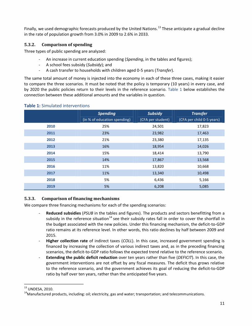
The same total amount of money is injected into the economy in each of these three cases, making it easier to compare the three scenarios. It must be noted that the policy is temporary (10 years) in every case, and by 2020 the public policies return to their levels in the reference scenario. Table 1 below establishes the connection between these additional amounts and the variables in question.
Table 1: Simulated interventions
Spending
(in % of education spending)
Subsidy
(CFA per student)
Transfer
(CFA per child 0-5 years)
2010 25% 24,501 17,823
2011 23% 23,982 17,463
2012 21% 23,380 17,135
2013 16% 18,954 14,026
2014 15% 18,414 13,790
2015 14% 17,867 13,568
2016 11% 13,820 10,668
2017 11% 13,340 10,498
2018 5% 6,436 5,166
2019 5% 6,208 5,085
5.3.3. Comparison of financing mechanisms
We compare three financing mechanisms for each of the spending scenarios:
- Reduced subsidies (PSUB in the tables and figures). The products and sectors benefitting from a subsidy in the reference situation14 see their subsidy rates fall in order to cover the shortfall in the budget associated with the new policies. Under this financing mechanism, the deficit-to-GDP ratio remains at its reference level. In other words, this ratio declines by half between 2009 and 2015.
- Higher collection rate of indirect taxes (COLL). In this case, increased government spending is financed by increasing the collection of various indirect taxes and, as in the preceding financing scenarios, the deficit-to-GDP ratio follows the expected trend relative to the reference scenario.
- Extending the public deficit reduction over ten years rather than five (DEFICIT). In this case, the government interventions are not offset by any fiscal measures. The deficit thus grows relative to the reference scenario, and the government achieves its goal of reducing the deficit-to-GDP ratio by half over ten years, rather than the anticipated five years.
13 UNDESA, 2010. 14Manufactured products, including: oil; electricity, gas and water; transportation; and telecommunications.
12
6. Analysis of results
6.1. Increase in public education spending
We begin here with a discussion of the effects of this simulation on education, the economy and poverty without consideration of the financing mechanism. Qualitatively, the results essentially go in the same direction and can be explained by the same transmission channels. We close the analysis of this scenario by comparing financing mechanisms.
6.1.1. Impact on education
In brief:
- An increase in education spending increases school participation and pass rates, leading to a primary school net enrolment ratio of nearly 5 percentage points more than in the reference scenario.
- Education spending induces further studies at the second level, where the number of students increased markedly (17 percent higher than in the reference scenario).
- The end of the program has a temporary negative impact on the various participation rates; these are slightly higher than they would have otherwise been in the long run.
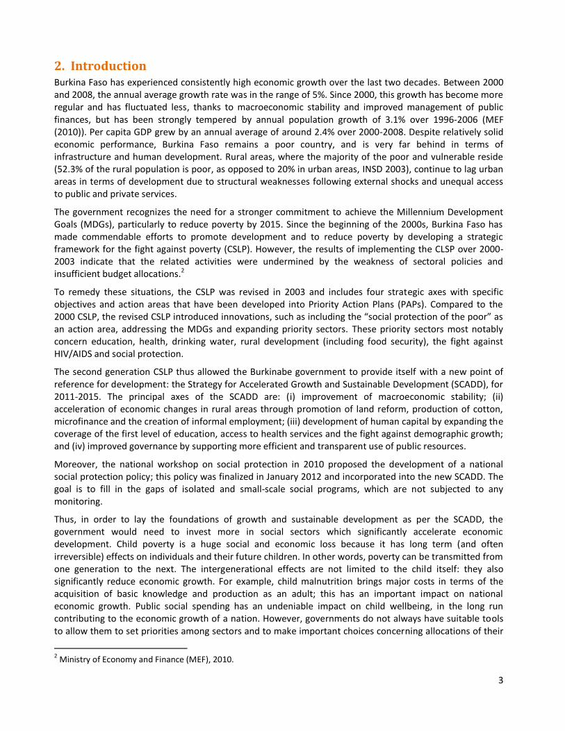
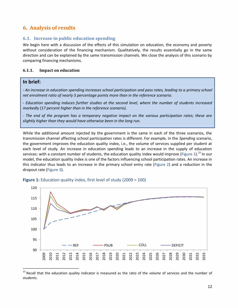
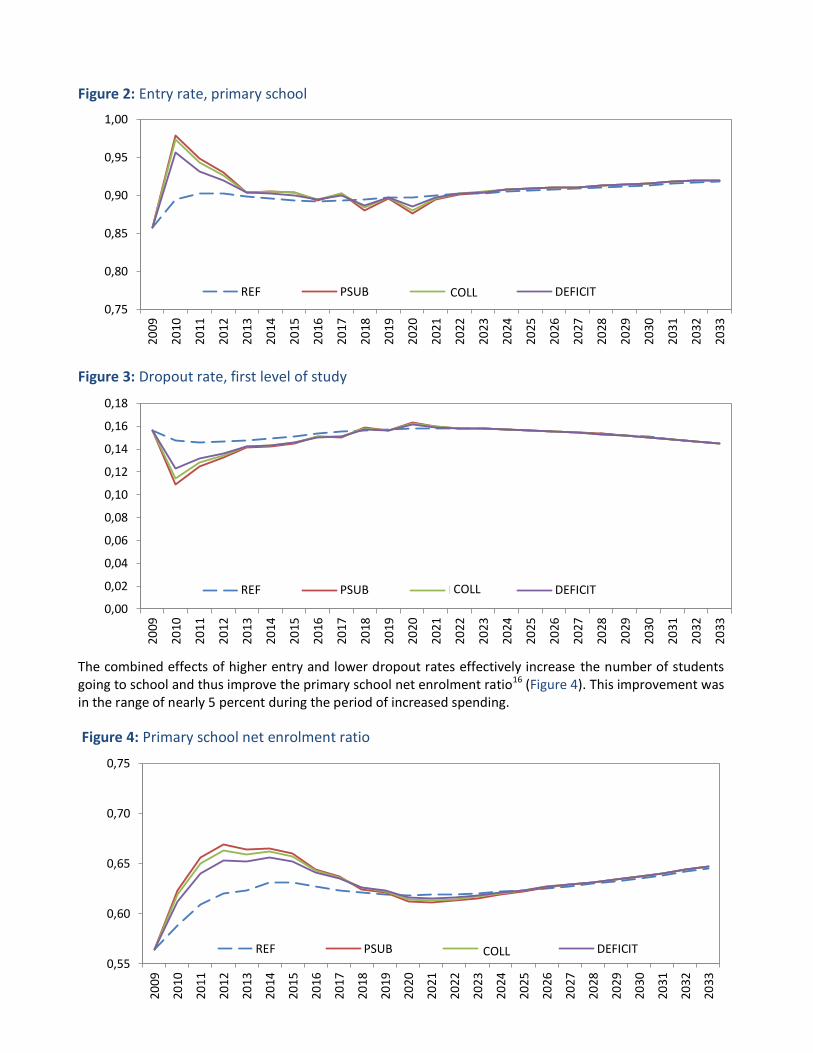
While the additional amount injected by the government is the same in each of the three scenarios, the transmission channel affecting school participation rates is different. For example, in the Spending scenario, the government improves the education quality index, i.e., the volume of services supplied per student at each level of study. An increase in education spending leads to an increase in the supply of education services: with a constant number of students, the education quality index would improve (Figure 1).15 In our model, the education quality index is one of the factors influencing school participation rates. An increase in this indicator thus leads to an increase in the primary school entry rate (Figure 2) and a reduction in the dropout rate (Figure 3).
Figure 1: Education quality index, first level of study (2009 = 100)
15 Recall that the education quality indicator is measured as the ratio of the volume of services and the number of students.
90
95
100
105
110
115
120
2009
2010
2011
2012
2013
2014
2015
2016
2017
2018
2019
2020
2021
2022
2023
2024
2025
2026
2027
2028
2029
2030
2031
2032
2033
REF PSUB PERC DEFICITCOLL
13
Figure 2: Entry rate, primary school
Figure 3: Dropout rate, first level of study
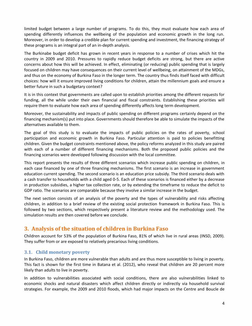
The combined effects of higher entry and lower dropout rates effectively increase the number of students going to school and thus improve the primary school net enrolment ratio16 (Figure 4). This improvement was in the range of nearly 5 percent during the period of increased spending.
Figure 5: Primary school net enrolment ratio
16 Here, this includes children aged 6-11 years who attend school.
0,75
0,80
0,85
0,90
0,95
1,00
2009
2010
2011
2012
2013
2014
2015
2016
2017
2018
2019
2020
2021
2022
2023
2024
2025
2026
2027
2028
2029
2030
2031
2032
2033
REF PSUB PERC DEFICIT
0,00
0,02
0,04
0,06
0,08
0,10
0,12
0,14
0,16
0,18
2009
2010
2011
2012
2013
2014
2015
2016
2017
2018
2019
2020
2021
2022
2023
2024
2025
2026
2027
2028
2029
2030
2031
2032
2033
REF PSUB PERC DEFICITCOLL
COLL
Figure 4: Primary school net enrolment ratio
0,55
0,60
0,65
0,70
0,75
2009
2010
2011
2012
2013
2014
2015
2016
2017
2018
2019
2020
2021
2022
2023
2024
2025
2026
2027
2028
2029
2030
2031
2032
2033
REF PSUB PERC DEFICITCOLL
14
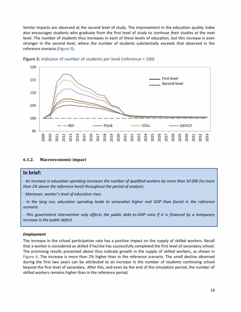
Similar impacts are observed at the second level of study. The improvement in the education quality index also encourages students who graduate from the first level of study to continue their studies at the next level. The number of students thus increases in each of these levels of education, but this increase is even stronger in the second level, where the number of students substantially exceeds that observed in the reference scenario (Figure 5).
Figure 5: Indicator of number of students per level (reference = 100)
6.1.2. Macroeconomic impact
In brief:
- An increase in education spending increases the number of qualified workers by more than 50 000 (to more than 2% above the reference level) throughout the period of analysis.
- Moreover, worker’s level of education rises.
- In the long run, education spending leads to somewhat higher real GDP than found in the reference scenario.
- This government intervention only affects the public debt-to-GDP ratio if it is financed by a temporary increase in the public deficit.
Employment
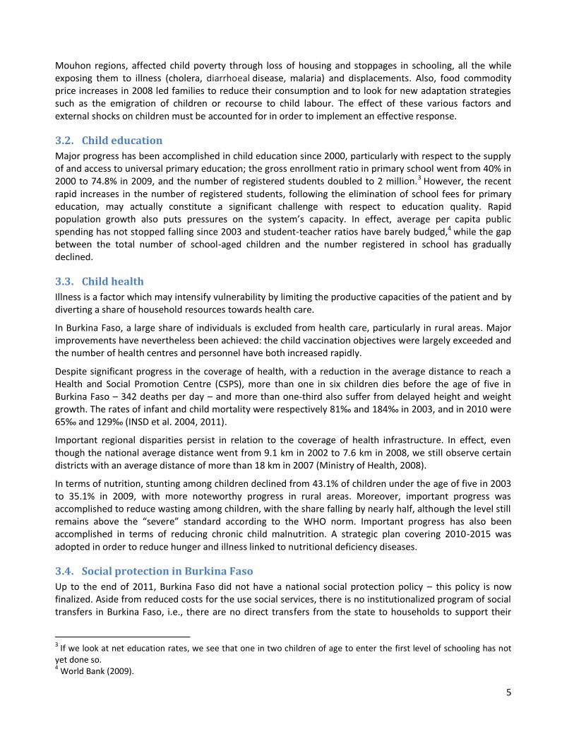
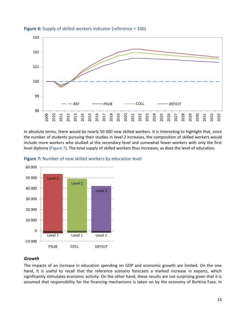
The increase in the school participation rate has a positive impact on the supply of skilled workers. Recall that a worker is considered as skilled if he/she has successfully completed the first level of secondary school. The promising results presented above thus indicate growth in the supply of skilled workers, as shown in Figure 6. The increase is more than 2% higher than in the reference scenario. The small decline observed during the first two years can be attributed to an increase in the number of students continuing school beyond the first level of secondary. After this, and even by the end of the simulation period, the number of skilled workers remains higher than in the reference period.
95
100
105
110
115
120
2009
2010
2011
2012
2013
2014
2015
2016
2017
2018
2019
2020
2021
2022
2023
2024
2025
2026
2027
2028
2029
2030
2031
2032
2033
REF PSUB PERC DEFICIT
First level Second level
COLL
15
Figure 6: Supply of skilled workers indicator (reference = 100)
In absolute terms, there would be nearly 50 000 new skilled workers. It is interesting to highlight that, since the number of students pursuing their studies in level 2 increases, the composition of skilled workers would include more workers who studied at the secondary level and somewhat fewer workers with only the first level diploma (Figure 7). The total supply of skilled workers thus increases, as does the level of education.
Figure 7: Number of new skilled workers by education level
Growth
The impacts of an increase in education spending on GDP and economic growth are limited. On the one hand, it is useful to recall that the reference scenario forecasts a marked increase in exports, which significantly stimulates economic activity. On the other hand, these results are not surprising given that it is assumed that responsibility for the financing mechanisms is taken on by the economy of Burkina Faso. In
98
99
100
101
102
103
2009
2010
2011
2012
2013
2014
2015
2016
2017
2018
2019
2020
2021
2022
2023
2024
2025
2026
2027
2028
2029
2030
2031
2032
2033
REF PSUB PERC DEFICIT
Level 1 Level 1 Level 1
Level 2 Level 2
Level 2
-10 000
0
10 000
20 000
30 000
40 000
50 000
60 000
PSUB PERC DEFICIT
COLL
COLL
16
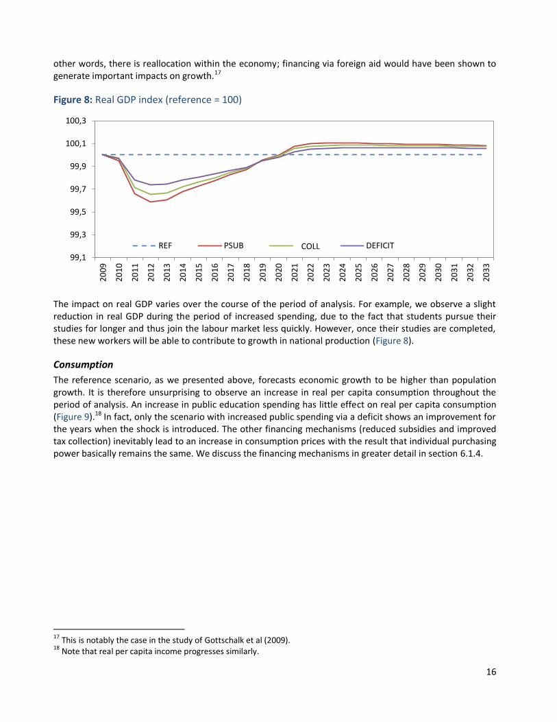
other words, there is reallocation within the economy; financing via foreign aid would have been shown to generate important impacts on growth.17
Figure 8: Real GDP index (reference = 100)
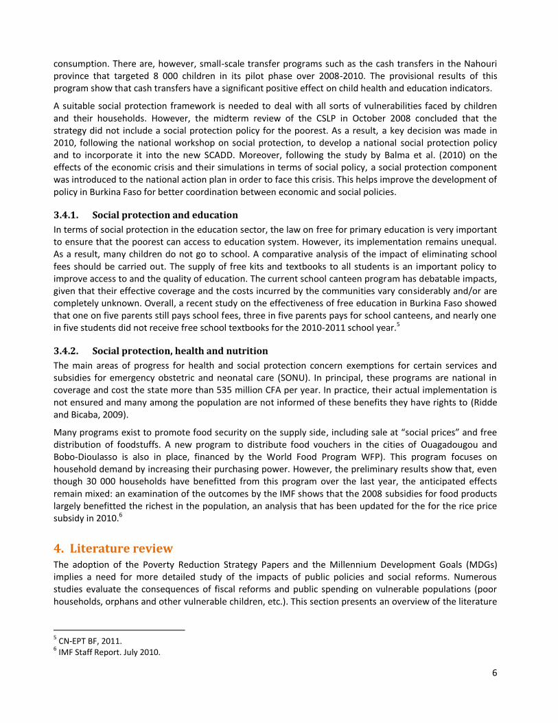
The impact on real GDP varies over the course of the period of analysis. For example, we observe a slight reduction in real GDP during the period of increased spending, due to the fact that students pursue their studies for longer and thus join the labour market less quickly. However, once their studies are completed, these new workers will be able to contribute to growth in national production (Figure 8).
Consumption
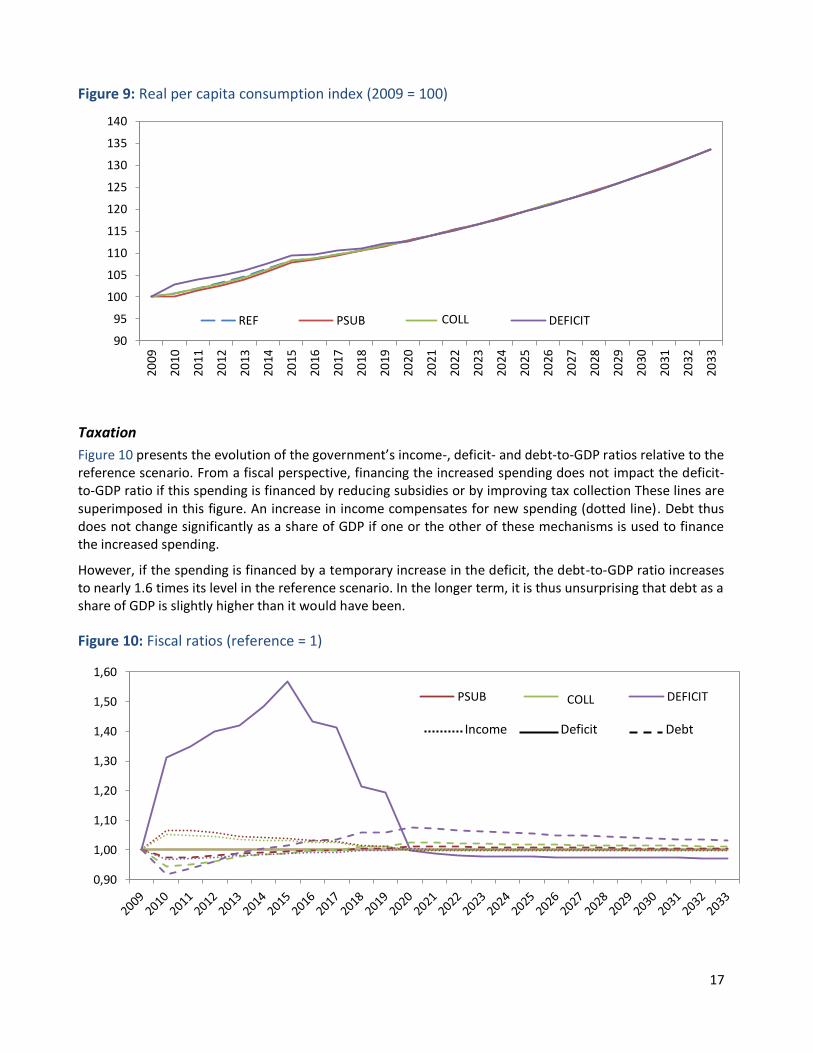
The reference scenario, as we presented above, forecasts economic growth to be higher than population growth. It is therefore unsurprising to observe an increase in real per capita consumption throughout the period of analysis. An increase in public education spending has little effect on real per capita consumption (Figure 9).18 In fact, only the scenario with increased public spending via a deficit shows an improvement for the years when the shock is introduced. The other financing mechanisms (reduced subsidies and improved tax collection) inevitably lead to an increase in consumption prices with the result that individual purchasing power basically remains the same. We discuss the financing mechanisms in greater detail in section 6.1.4.
17 This is notably the case in the study of Gottschalk et al (2009). 18 Note that real per capita income progresses similarly.
99,1
99,3
99,5
99,7
99,9
100,1
100,3
2009
2010
2011
2012
2013
2014
2015
2016
2017
2018
2019
2020
2021
2022
2023
2024
2025
2026
2027
2028
2029
2030
2031
2032
2033
REF PSUB PERC DEFICITCOLL
17
Figure 9: Real per capita consumption index (2009 = 100)
Taxation
Figure 10 presents the evolution of the government’s income-, deficit- and debt-to-GDP ratios relative to the reference scenario. From a fiscal perspective, financing the increased spending does not impact the deficit-to-GDP ratio if this spending is financed by reducing subsidies or by improving tax collection These lines are superimposed in this figure. An increase in income compensates for new spending (dotted line). Debt thus does not change significantly as a share of GDP if one or the other of these mechanisms is used to finance the increased spending.
However, if the spending is financed by a temporary increase in the deficit, the debt-to-GDP ratio increases to nearly 1.6 times its level in the reference scenario. In the longer term, it is thus unsurprising that debt as a share of GDP is slightly higher than it would have been.
Figure 10: Fiscal ratios (reference = 1)
90
95
100
105
110
115
120
125
130
135
140
2009
2010
2011
2012
2013
2014
2015
2016
2017
2018
2019
2020
2021
2022
2023
2024
2025
2026
2027
2028
2029
2030
2031
2032
2033
REF PSUB PERC DEFICIT
0,90
1,00
1,10
1,20
1,30
1,40
1,50
1,60
PSUB PERC DEFICIT
Série1 Série2 Série3 Income Deficit Debt
COLL
COLL
18
6.1.3. Impact on poverty
In brief:
- In the long run, all poverty indicators decline markedly in the reference scenario.
- An increase in public education spending reduces monetary and caloric poverty, particularly during the intervention period, but only if this spending is financed by an increase in the deficit.
The simulation results from the computable general equilibrium model – particularly those related to wage rates, employment of skilled and unskilled workers, production and consumption prices, and sectoral value added – are introduced in a microsimulation model of household and individual behaviour to forecast the impacts on child monetary and caloric poverty. It is important to highlight that the equivalence scales used in this study (adult equivalent according to caloric needs) differ from those used in the official estimates. This having been said, the estimates presented below are not comparable with the official number. The caloric and monetary poverty lines were determined in terms of the needs of children aged 0-17. This explains why the child poverty rates are lower than poverty when using the lines set for the population as a whole.
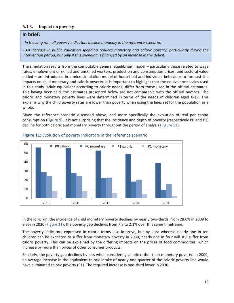
Given the reference scenario discussed above, and more specifically the evolution of real per capita consumption (Figure 9), it is not surprising that the incidence and depth of poverty (respectively P0 and P1) decline for both caloric and monetary poverty throughout the period of analysis (Figure 11).
Figure 11: Evolution of poverty indicators in the reference scenario
In the long run, the incidence of child monetary poverty declines by nearly two-thirds, from 28.6% in 2009 to 9.3% in 2030 (Figure 11); the poverty gap declines from 7.8 to 2.1% over this same timeframe.
The poverty indicators expressed in caloric terms also improve, but by less: whereas nearly one in ten children can be expected to suffer from monetary poverty in 2030, nearly one in four will still suffer from caloric poverty. This can be explained by the differing impacts on the prices of food commodities, which increase by more than prices of other consumer products.
Similarly, the poverty gap declines by less when considering caloric rather than monetary poverty. In 2009, an average increase in the equivalent caloric intake of nearly one-quarter of the caloric poverty line would have eliminated caloric poverty (P1). The required increase is one-third lower in 2030.
0
10
20
30
40
50
60
2009 2010 2015 2020 2030
P0 calorique P0 monétaire P1 calorique P1 monétaireP0 caloric P0 monetary P1 caloric P0 caloric
0
10
20
30
40
50
60
2009 2010 2015 2020 2030
P0 calorique P0 monétaire P1 calorique P1 monétaireP0 caloric P0 monetary P1 caloric P1 monetary
19
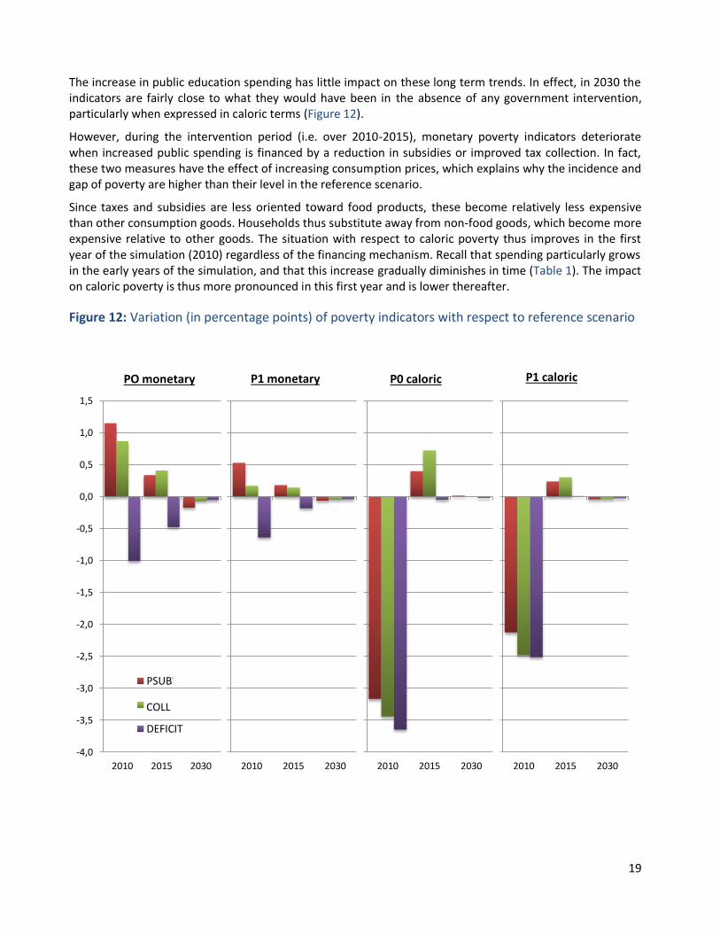
The increase in public education spending has little impact on these long term trends. In effect, in 2030 the indicators are fairly close to what they would have been in the absence of any government intervention, particularly when expressed in caloric terms (Figure 12).
However, during the intervention period (i.e. over 2010-2015), monetary poverty indicators deteriorate when increased public spending is financed by a reduction in subsidies or improved tax collection. In fact, these two measures have the effect of increasing consumption prices, which explains why the incidence and gap of poverty are higher than their level in the reference scenario.
Since taxes and subsidies are less oriented toward food products, these become relatively less expensive than other consumption goods. Households thus substitute away from non-food goods, which become more expensive relative to other goods. The situation with respect to caloric poverty thus improves in the first year of the simulation (2010) regardless of the financing mechanism. Recall that spending particularly grows in the early years of the simulation, and that this increase gradually diminishes in time (Table 1). The impact on caloric poverty is thus more pronounced in this first year and is lower thereafter.
Figure 12: Variation (in percentage points) of poverty indicators with respect to reference scenario
-4,00
-3,50
-3,00
-2,50
-2,00
-1,50
-1,00
-0,50
0,00
0,50
1,00
1,50
2010 2015 2030
-4,00
-3,50
-3,00
-2,50
-2,00
-1,50
-1,00
-0,50
0,00
0,50
1,00
1,50
2010 2015 2030
-4,00
-3,50
-3,00
-2,50
-2,00
-1,50
-1,00
-0,50
0,00
0,50
1,00
1,50
2010 2015 2030
P1 mon
-4,0
-3,5
-3,0
-2,5
-2,0
-1,5
-1,0
-0,5
0,0
0,5
1,0
1,5
2010 2015 2030
P0 monétaire
PSUBV
PERC
DEFICIT
PO monetary P1 monetary P0 caloric P1 caloric
COLL
20
6.1.4. Comparison of financing mechanisms
In brief:
- The additional financing via taxation has slightly larger impacts on education and economic activity, but increases monetary poverty in the medium term.
- Financing the spending with a temporary increase in the deficit is the mechanism leading to the greatest reduction of monetary and caloric poverty in the medium term.
The impact of an increase in public education spending is qualitatively similar, regardless of the financing mechanism. Compared to the reference scenario, the school participation and pass rates improve, the supply of skilled labour increases and economic activity is stimulated.
Financing this new spending by reducing existing subsidies, however, leads to slightly higher levels of each of these indicators; the effect is similar, although smaller, when improved tax collection finances the spending. As discussed above, both of these financing mechanisms raise the overall price level. Since the price of education is not affected by these two mechanisms, neither reduced subsidies nor increased tax collection have a direct impact on education: the impact is thus felt through a relative change in prices, where the real price of education in the consumer’s deflated basket declines, thus promoting school participation and pass rates, along with the ensuing macroeconomic effects.
The opposite is observed in terms of the impacts on poverty. Only financing the additional spending through an increase in the deficit reduces poverty rates significantly in the medium term. In the longer term, monetary poverty falls regardless of the financing mechanisms used, and the reduction is greater in both cases other than the increased deficit. These differences are barely perceptible for caloric poverty.
These results were observed for all intervention types. In the following analysis, we solely focus on comparison of the three intervention types under one single financing mechanism, namely the deficit. The reader should nevertheless keep in mind the slightly differentiated impacted of the other financing mechanisms.
6.2. Comparison of intervention types
6.2.1. Impact on education
In brief:
- Education spending improves both school participation and pass rates.
- A school fees subsidy mostly affects the primary school entry rate, with limited effects on other educational behaviours.
- A cash transfer to households has little impact on educational behaviours.
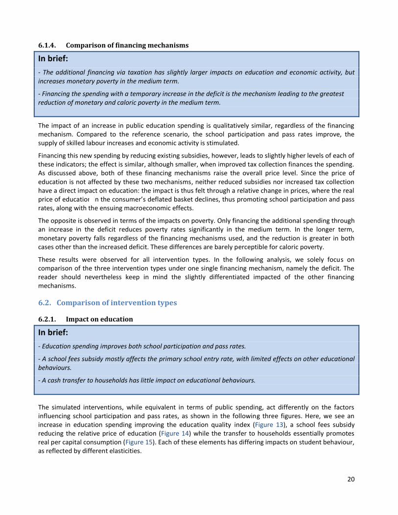
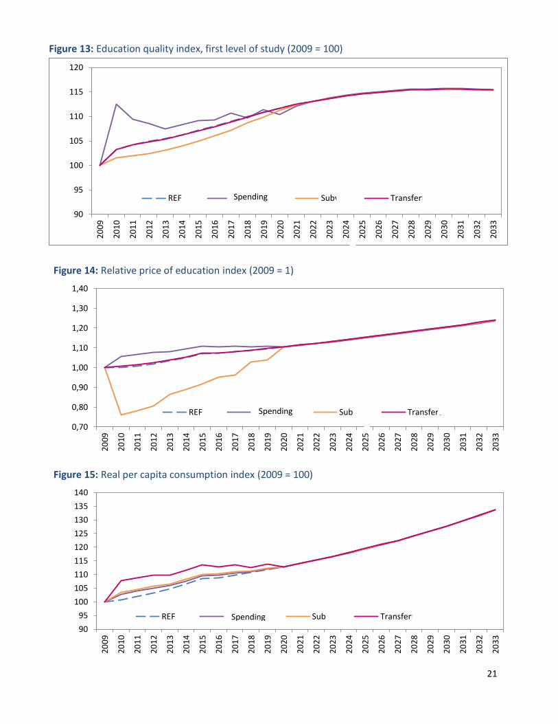
The simulated interventions, while equivalent in terms of public spending, act differently on the factors influencing school participation and pass rates, as shown in the following three figures. Here, we see an increase in education spending improving the education quality index (Figure 13), a school fees subsidy reducing the relative price of education (Figure 14) while the transfer to households essentially promotes real per capital consumption (Figure 15). Each of these elements has differing impacts on student behaviour, as reflected by different elasticities.
21
Figure 14: Relative price of education index (2009 = 1)
Figure 15: Real per capita consumption index (2009 = 100)
0,70
0,80
0,90
1,00
1,10
1,20
1,30
1,40
2009
2010
2011
2012
2013
2014
2015
2016
2017
2018
2019
2020
2021
2022
2023
2024
2025
2026
2027
2028
2029
2030
2031
2032
2033
REF Dépenses Subv Transfert
90
95
100
105
110
115
120
125
130
135
140
2009
2010
2011
2012
2013
2014
2015
2016
2017
2018
2019
2020
2021
2022
2023
2024
2025
2026
2027
2028
2029
2030
2031
2032
2033
REF Dépenses Subv Transfert
Figure 13: Education quality index, first level of study (2009 = 100)
90
95
100
105
110
115
120
2009
2010
2011
2012
2013
2014
2015
2016
2017
2018
2019
2020
2021
2022
2023
2024
2025
2026
2027
2028
2029
2030
2031
2032
2033
REF Dépenses Subv TransfertSpending
Spending
Spending
22
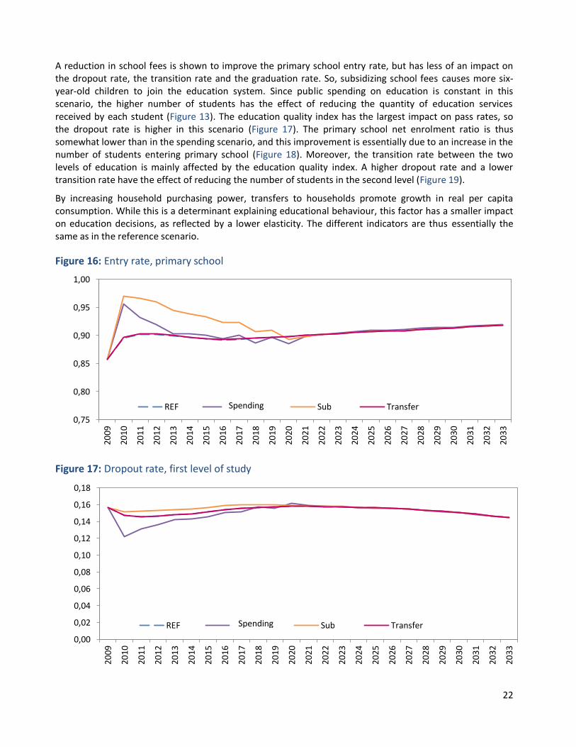
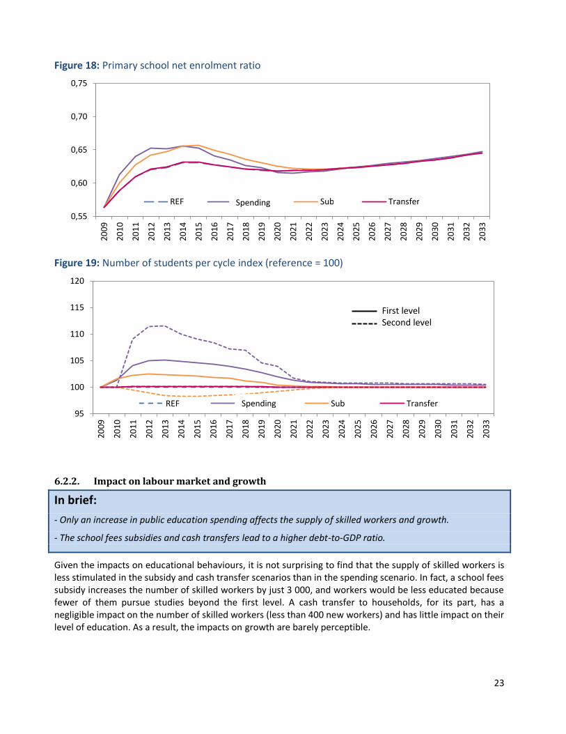
A reduction in school fees is shown to improve the primary school entry rate, but has less of an impact on the dropout rate, the transition rate and the graduation rate. So, subsidizing school fees causes more six-year-old children to join the education system. Since public spending on education is constant in this scenario, the higher number of students has the effect of reducing the quantity of education services received by each student (Figure 13). The education quality index has the largest impact on pass rates, so the dropout rate is higher in this scenario (Figure 17). The primary school net enrolment ratio is thus somewhat lower than in the spending scenario, and this improvement is essentially due to an increase in the number of students entering primary school (Figure 18). Moreover, the transition rate between the two levels of education is mainly affected by the education quality index. A higher dropout rate and a lower transition rate have the effect of reducing the number of students in the second level (Figure 19).
By increasing household purchasing power, transfers to households promote growth in real per capita consumption. While this is a determinant explaining educational behaviour, this factor has a smaller impact on education decisions, as reflected by a lower elasticity. The different indicators are thus essentially the same as in the reference scenario.
Figure 16: Entry rate, primary school
Figure 17: Dropout rate, first level of study
0,75
0,80
0,85
0,90
0,95
1,00
2009
2010
2011
2012
2013
2014
2015
2016
2017
2018
2019
2020
2021
2022
2023
2024
2025
2026
2027
2028
2029
2030
2031
2032
2033
REF Dépenses Subv Transfert
0,00
0,02
0,04
0,06
0,08
0,10
0,12
0,14
0,16
0,18
2009
2010
2011
2012
2013
2014
2015
2016
2017
2018
2019
2020
2021
2022
2023
2024
2025
2026
2027
2028
2029
2030
2031
2032
2033
REF Dépenses Subv TransfertSpending
Spending
23
Figure 18: Primary school net enrolment ratio
Figure 19: Number of students per cycle index (reference = 100)
6.2.2. Impact on labour market and growth
In brief:
- Only an increase in public education spending affects the supply of skilled workers and growth.
- The school fees subsidies and cash transfers lead to a higher debt-to-GDP ratio.
Given the impacts on educational behaviours, it is not surprising to find that the supply of skilled workers is less stimulated in the subsidy and cash transfer scenarios than in the spending scenario. In fact, a school fees subsidy increases the number of skilled workers by just 3 000, and workers would be less educated because fewer of them pursue studies beyond the first level. A cash transfer to households, for its part, has a negligible impact on the number of skilled workers (less than 400 new workers) and has little impact on their level of education. As a result, the impacts on growth are barely perceptible.
0,55
0,60
0,65
0,70
0,75
2009
2010
2011
2012
2013
2014
2015
2016
2017
2018
2019
2020
2021
2022
2023
2024
2025
2026
2027
2028
2029
2030
2031
2032
2033
REF Dépenses Subv Transfert
95
100
105
110
115
120
2009
2010
2011
2012
2013
2014
2015
2016
2017
2018
2019
2020
2021
2022
2023
2024
2025
2026
2027
2028
2029
2030
2031
2032
2033
REF Dépenses Subv Transfert
First level Second level
Spending
Spending
24
Figure 20: Supply of qualified workers index (reference = 100)
Figure 21: Number of skilled workers by education level
Figure 22: Real GDP index (reference = 100)
98
99
100
101
102
103
2009
2010
2011
2012
2013
2014
2015
2016
2017
2018
2019
2020
2021
2022
2023
2024
2025
2026
2027
2028
2029
2030
2031
2032
2033
REF Dépenses Subv Transfert
Level 1
Level 1
Level 1
Level 2
Level 2
Level 2
-10 000
0
10 000
20 000
30 000
40 000
50 000
Dépenses Subv Transfert
99,1
99,3
99,5
99,7
99,9
100,1
100,3
2009
2010
2011
2012
2013
2014
2015
2016
2017
2018
2019
2020
2021
2022
2023
2024
2025
2026
2027
2028
2029
2030
2031
2032
2033
REF Dépenses Subv Transfert
Spending
Spending
Spending
25
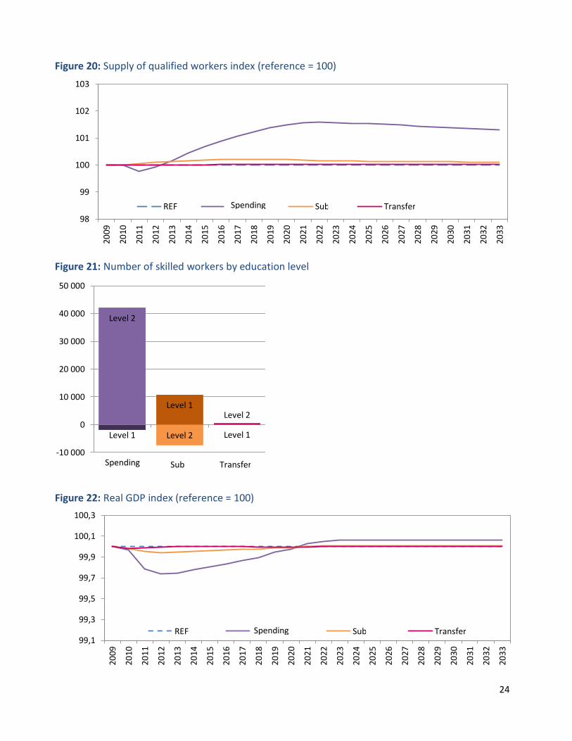
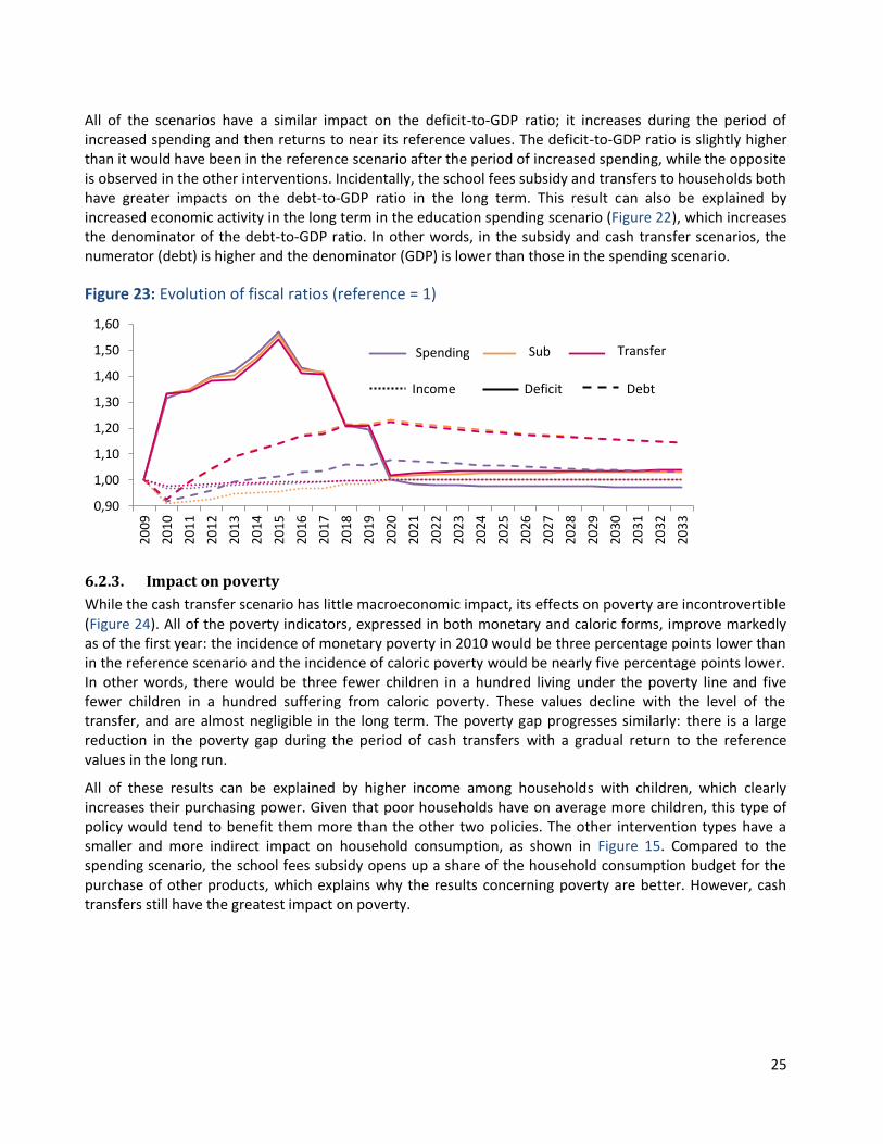
All of the scenarios have a similar impact on the deficit-to-GDP ratio; it increases during the period of increased spending and then returns to near its reference values. The deficit-to-GDP ratio is slightly higher than it would have been in the reference scenario after the period of increased spending, while the opposite is observed in the other interventions. Incidentally, the school fees subsidy and transfers to households both have greater impacts on the debt-to-GDP ratio in the long term. This result can also be explained by increased economic activity in the long term in the education spending scenario (Figure 22), which increases the denominator of the debt-to-GDP ratio. In other words, in the subsidy and cash transfer scenarios, the numerator (debt) is higher and the denominator (GDP) is lower than those in the spending scenario.
Figure 23: Evolution of fiscal ratios (reference = 1)
6.2.3. Impact on poverty
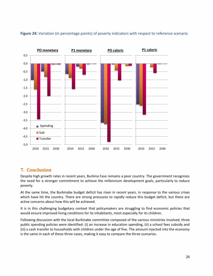
While the cash transfer scenario has little macroeconomic impact, its effects on poverty are incontrovertible (Figure 24). All of the poverty indicators, expressed in both monetary and caloric forms, improve markedly as of the first year: the incidence of monetary poverty in 2010 would be three percentage points lower than in the reference scenario and the incidence of caloric poverty would be nearly five percentage points lower. In other words, there would be three fewer children in a hundred living under the poverty line and five fewer children in a hundred suffering from caloric poverty. These values decline with the level of the transfer, and are almost negligible in the long term. The poverty gap progresses similarly: there is a large reduction in the poverty gap during the period of cash transfers with a gradual return to the reference values in the long run.
All of these results can be explained by higher income among households with children, which clearly increases their purchasing power. Given that poor households have on average more children, this type of policy would tend to benefit them more than the other two policies. The other intervention types have a smaller and more indirect impact on household consumption, as shown in Figure 15. Compared to the spending scenario, the school fees subsidy opens up a share of the household consumption budget for the purchase of other products, which explains why the results concerning poverty are better. However, cash transfers still have the greatest impact on poverty.
0,90
1,00
1,10
1,20
1,30
1,40
1,50
1,60
2009
2010
2011
2012
2013
2014
2015
2016
2017
2018
2019
2020
2021
2022
2023
2024
2025
2026
2027
2028
2029
2030
2031
2032
2033
Dépenses Subv TransfertTransfer Sub Spending
Income Deficit Debt
26
Figure 24: Variation (in percentage points) of poverty indicators with respect to reference scenario
7. Conclusion Despite high growth rates in recent years, Burkina Faso remains a poor country. The government recognizes the need for a stronger commitment to achieve the millennium development goals, particularly to reduce poverty.
At the same time, the Burkinabe budget deficit has risen in recent years, in response to the various crises which have hit the country. There are strong pressures to rapidly reduce this budget deficit, but there are active concerns about how this will be achieved.
It is in this challenging budgetary context that policymakers are struggling to find economic policies that would ensure improved living conditions for its inhabitants, most especially for its children.
Following discussion with the local Burkinabe committee composed of the various ministries involved, three public spending policies were identified: (i) an increase in education spending, (ii) a school fees subsidy and (iii) a cash transfer to households with children under the age of five. The amount injected into the economy is the same in each of these three cases, making it easy to compare the three scenarios.
-5,00
-4,50
-4,00
-3,50
-3,00
-2,50
-2,00
-1,50
-1,00
-0,50
0,00
0,50
2010 2015 2030
P1 calorique
-5,00
-4,50
-4,00
-3,50
-3,00
-2,50
-2,00
-1,50
-1,00
-0,50
0,00
0,50
2010 2015 2030
P0 calorique
-5,00
-4,50
-4,00
-3,50
-3,00
-2,50
-2,00
-1,50
-1,00
-0,50
0,00
0,50
2010 2015 2030
P1 monétaire
-5,0
-4,5
-4,0
-3,5
-3,0
-2,5
-2,0
-1,5
-1,0
-0,5
0,0
0,5
2010 2015 2030
P0 monétaire
Dépenses
Subv
Transfert
PO monetary P1 monetary PO caloric P1 caloric
Spending
27
The discussion also made it possible to identify the three most realistic financing mechanisms: (i) an increase in subsidies, (ii) an increase in the indirect tax collection rate and (iii) an extension of the time to reduce the public deficit to ten years rather than five.
We used a dynamic computable general equilibrium model together with a microeconomic model to evaluate the impacts of these three policies under three different financing mechanisms. Relative to the reference scenario, the results indicate that higher public education spending increases school participation and pass rates, leading to an increased supply and education level of skilled workers, all in turn leading to a lower incidence and depth of both monetary and caloric poverty.
The school fees subsidies have more differentiated impacts on education, with a larger beneficial impact on primary school entry and a smaller impact on continuation of their studies. Finally, the supply of skilled workers increases slightly, but the education level of these workers is lower than in the reference scenario. This type of intervention thus also has a positive impact on poverty, and the impacts in this case are more pronounced than in the case of public education spending.
As for the cash transfers, they have a minimal impact on educational behaviours, and thus on the supply of skilled workers, but they significantly reduce the incidence and severity of poverty.
These results are qualitatively similar regardless of the financing approach. Moreover, the financing mechanism does not appear to have a significant impact on macroeconomic and fiscal indicators in the long term, particularly in the case of public education spending. For the other intervention types, the debt-to-GDP ratio would be higher than in the reference scenario. This having been said, financing the state interventions through a reduction in subsidies or improved tax collection would have negative impacts on poverty, because these measures increase the price level.
In summary, if the objective is to achieve improved educational and economic performance, it seems as though the best approach to the intervention would be to increase public education spending. However, cash transfers to families would be more suitable if reducing child poverty is instead prioritized. Regardless of the intervention(s) ultimately adopted, the most suitable financing mechanism appears to be a temporary increase in the public deficit since this generates smaller negative impacts on the quality of life of the most destitute.

28
8. References
Ahmad E. and N. Stern (1984). The Theory of Reform and Indian Indirect Taxes. Journal of Public Economics, 25:3:259-298.
Alderman, H. and C. Del Ninno (1999). Poverty issues for zero rating VAT in South Africa. Journal of African Economies, 8:2:182-208.
Balma, L., J. Cockburn, I. Fofana L. Tiberti and S. Kabore (2010). Analyse d’impact des effets de crise économique et des politiques de réponse sur les enfants en Afrique de l’Ouest et du Centre: Cas du Burkina Faso (Impact analysis of the effects of the economic crisis and policy responses on children in West and Central Africa: case of Burkina Faso). Innocenti Working Paper No. 2010-03.
Batana, Y., J. Cockburn and H. J-L. Guene (2012). Analyse de la situation de la pauvreté et de la vulnérabilité de l’enfant et de la femme au Burkina Faso (Analysis of the situation of poverty and vulnerability of children and women). Report commissioned by UNICEF-Burkina Faso, forthcoming.
Bibi, S. and J-Y. Duclos (2004). Réformes Fiscales et Réduction de la Pauvreté: Application sur des Données Tunisiennes (Fiscal reforms and poverty reduction: An application to Tunisian data).
Boccanfuso D., F. Cissé, A. Diagne and L. Savard (2003). Un modèle CGE-Multi-Ménages Intégrés Appliqué à l’économie sénégalaise (An integrated multi-household CGE model applied to the Senegalese economy). Mimeo, CREA, Dakar.
Bourguignon, F., A.S. Robilliard and S. Robinson (2003). Representative versus real households in the macroeconomic modeling of inequality, DT/2003/10, DIAL/Unité de recherche CIRPEE.
Chen, D., J. Matovu and R. Reinikka (2001). A Quest for Revenue and Tax Incidence, in Reinikka, Ritva, and Paul Collier (eds.) Uganda’s Recovery: The Role of Farms, Firms, and Government. World Bank: Washington DC.
CN-EPT BF (2011). The effectiveness of the education subsidy in Burkina Faso (L’effectivité de la gratuité de l’éducation au Burkina Faso). Coalition Nationale pour la Education Pour Tous.
Cockburn, J. (2006), Trade Liberalisation and Poverty in Nepal: A Computable General Equilibrium Micro Simulation Analysis, in Maurizio Bussolo and Jeffery Round (eds.), Globalization and Poverty: Channels and Policies. Routledge: London.
Cockburn, J., H. Maisonnave, Robichaud, V. and L. Tiberti (2012). Espace fiscal et dépenses publiques pour les enfants au Burkina Faso – Rapport technique (Fiscal space and public spending on children in Burkina Faso – Technical Report). Mimeo.
Cogneau D. and A.-S. Robilliard (2001). Growth, distribution and poverty in Madagascar: Learning from a Microsimulation Model in a General Equilibrium Framework. IFPRI TMD Discussion paper No. 61 and DIAL DT/2001-19.
Cogneau D.and A.-S. Robilliard (2004). Poverty Alleviation Policy in Madagascar: A Micro-Macro Simulation Model. DT/2004/11, DIAL/Unité de recherche CIRPEE.
Decaluwé B., J.C. Dumont. and L. Savard (1999), Measuring poverty and inequality in a Computable general equilibrium framework. Université Laval, Cahier de recherche du CREFA no 99-20.
Gertler, P. and J. Van Der Gaag (1990). The willingness to pay for medical care: Evidence from two developing countries. The John Hopkins University Press: Baltimore.
Glewwe, P. (1991). Investigating the Determinants of Household welfare in Côte d’Ivoire. Journal of Development Economics, 35:307-337.
Gottschalk, J., Manh Vu Le, H. Lofgren and K. Nouve (2009). Analyzing Fiscal Space Using MAMS: An Application to Burkina Faso. IMF working paper WP/09/227.
29
International Monetary Fund (2010). Burkina Faso: Request for a Three-Year Arrangement Under the Extended Credit Facility—Staff Report; Staff Supplement; Press Release on the Executive Board Discussion; and Statement by the Executive Director for Burkina Faso, IMF Country Report 10/197.
International Monetary Fund (2011). Burkina Faso: Deuxième revue de l’accord triennal au titre de la facilité élargie de crédit et demande de modification de critères de réalisation - Rapport des services du FMI (Second review of the triennial agreement on the expanded credit facility and the request to modify the performance criteria): press release relating to the proceedings of the board; and, statement of the IMF executive director for Burkina Faso, IMF Country Report 11/226, available at: http://www.imf.org/external/french/pubs/ft/scr/2011/cr11226f.pdf
National Institute of Statistics and Demography (INSD), Ministry of Economy and Finance and ORC Macro (2003). Profil et Évolution de la Pauvreté au Burkina Faso (Profile and evolution of poverty in Burkina Faso). Ministry of Economic and Finance, General Directorate of Statistics, Ouagadougou.
National Institute of Statistics and Demography (INSD), Ministry of Economy and Finance and ORC Macro (2004). 2003 Burkina Faso demographic and health survey. Calverton, Maryland, USA: INSD and ORC Macro.
National Institute of Statistics and Demography (INSD), Ministry of Economy and Finance and ORC Macro (2009). Rapport provisoire de l’enquête Burkinabè sur les conditions des ménages (Provisory report on the Burkinabe survey on household living conditions).
National Institute of Statistics and Demography (INSD), Ministry of Economy and Finance and ORC Macro (2011). 2010 Burkina Faso demographic and health survey. Calverton, Maryland, USA: INSD and ORC Macro. Preliminary report.
Lofgren, H and C. Diaz-Bonilla (2006). MAMS: An Economy-wide Model for Analysis of MDG Country Strategies. Technical Documentation, DECPG, World Bank.
Makdissi, P. and Q. Wodon (2002). Consumption Dominance Curves: Testing for the Impact of Indirect Tax Reforms on Poverty. Economics Letters, 75:227-235.
Mayshar, J., and S. Yitzhaki (1996). Dalton-improving tax reform: When households differ in ability and needs. Journal of Public Economics, 62:399-412.
Ministry of Health (2008). Maternal, neonatal and child mortality, May 2008 project document. Ministry of Health and Partnership for Maternal, Newborn and Child Health.
Ministry of Economy and Finance (2010). Progrès et acquis du développement du Burkina Faso 2000-2009 (Development progress and gains in Burkina Faso, 2000-2009).
Ministry of Primary Education and Literacy (2010). Statistiques de l’éducation de base 2009-2010 (Primary education statistics, 2009-2010). Directorate of studies and planning, available online at: http://www.cns.bf/IMG/pdf/Annuaire_2009_2010_MEBA.pdf
Ministry of Secondary and Higher Education and Scientific Research (2009) Annuaire statistique de l’enseignement secondaire 2008-2009 (Annual report on secondary education statistics). Directorate of studies and planning, available online at: http://www.messrs.gov.bf/SiteMessrs/statistiques/ANNUAIRE-2008-2009-SECONDAIRE.pdf
Rajemison, H. and S. D. Younger (2000). Indirect tax in Madagascar: Estimations using the input-output table. CFNPP Working Paper #106.
Ray, D. (1997). Development economics. Princeton University Press.
Ridde, V. and A. Bicaba (2009). Revue des politiques d’exemption/subvention du paiement au Burkina Faso La stratégie de subvention des soins obstétricaux et néonataux d’urgence (Review of payment exemptions/subsidies in Burkina Faso : The strategy of subsidizing obstetric and neonatal emergency care). Université de Montréal. SERSAP. Anvers: Institut de médecine tropicale d’Anvers and UNICEF.
30
Sahn, D. E. and S. D. Younger (2003). Estimating the Incidence of Indirect Taxes in Developing Countries, in Bourguignon, Francois and Luiz Pereira da Silva (eds.) Evaluating the poverty and distributional impact of economic policies. Oxford University Press: New York.
United Nations Department of Economics and Social Affairs (2010). World population prospects. Available on line at: http://esa.un.org/unpd/wpp/Excel-Data/population.htm
Waddington, L. (2004). Linking Economic Policy to Childhood Poverty: A review of the evidence on growth, trade reform and macroeconomic policy. CHIP Report No.7.
World Bank (2009). La Revue des Dépenses Publique dans le secteur de l’éducation (Public expenditure review in the education sector). Burkina Faso.
Yitzhaki, S. and J. Slemrod (1991). Welfare dominance: An application to commodity taxation. American Economic Review, 81:480-496.
Yitzhaki, S. and W. Thirsk (1990). Welfare Dominance and the Design of Excise Taxation in the Côte d'Ivoire. Journal of Development Economics, 33:1-18.