fiscal system analysis concessionary systems

8/10/2019 Fiscal System Analysis Concessionary Systems

http://slidepdf.com/reader/full/fiscal-system-analysis-concessionary-systems 1/13

Energy 32 (2007) 2135–2147

Fiscal system analysis—concessionary systems

Mark J. KaiserCenter for Energy Studies, Louisiana State University, Energy, Coast & Environment Building, Nicholson Extension Drive, Baton Rouge, LA 70803, USA

Received 17 January 2007

Abstract

The economic and system measures associated with hydrocarbon development are subject to various levels of private and marketuncertainty. The purpose of this paper is to develop an analytic framework to quantify the inuence of private and market uncertaintyunder a concessionary scal system. A meta-modeling approach is employed to develop regression models for take and investmentcriteria in terms of various exogenous, scal, and user-dened parameters. The critical assumptions involved in estimation, theuncertainty associated with interpretation, and the limitations of the analysis are examined. The deepwater Gulf of Mexico Na Kikadevelopment is considered as a case study.r 2007 Elsevier Ltd. All rights reserved.

Keywords: Computational modeling; Contract negotiation; Fiscal regimes; Meta-modeling

1. Introduction

The economics of the upstream petroleum businessis complex and dynamic. Each year a dozen or morecountries offer license rounds, introduce new modelcontracts or scal regimes, or revise their tax laws. Thereare more scal systems in the world than there arecountries producing oil and gas because numerous vintagesof contracts may be in force at any one time and contractterms often change as countries gain experience inlicensing, global economic conditions shift, or as theperception of prospectivity in a region change.

Governments decide whether resources are privatelyowned or whether they are State property. Under aconcessionary (royalty/tax) arrangement, the contract

holder secures exclusive exploration rights from a privateparty or government for a specied duration, as well as anexclusive development and production right for eachcommercial discovery. The concession was the rst systemused in world petroleum arrangements and can be traced tosilver mining operators in Greece in 480 B.C. [1]. Theearliest petroleum concessionary agreements consistedonly of a royalty. As governments gained experience and

bargaining power, contracts were renegotiated, royaltiesincreased, and various levels of taxation were added.Today, royalty/tax systems employ numerous scal devicesand sophisticated formulas to capture rent, and abouthalf of all active contracts are written as royalty/taxsystems. The United States employs a royalty/tax regime inoil and gas production licenses for onshore and offshoreproperties.

In the traditional concessionary system, the companypays a royalty, based on the value of the recovered mineralresources, and one or more taxes, based on taxable income.The royalty is normally a percentage of the gross revenuesof the sale of hydrocarbons and can be paid in cash or inkind. Royalty represents a cost of doing business and isthus tax-deductible. Other deductions typically include

operating cost, depreciation of capitalized assets, andamortization. The revenue that remains after the scalcost has been deducted is called taxable income. Taxes arepaid depending on the applicable rate and the after-tax netcash ow is determined which is used for protabilityassessment.

The purpose of this paper is to develop an analyticframework to quantify the inuence of private and marketuncertainty on the economic and system measures asso-ciated with eld development. A meta-modeling approachis employed to develop regression models for take and

ARTICLE IN PRESS

www.elsevier.com/locate/energy

0360-5442/$ - see front matter r 2007 Elsevier Ltd. All rights reserved.doi: 10.1016/j.energy.2007.04.013

Tel.: +1225 5784554; fax: +1 225578 4541.E-mail address: [email protected]

http://www.elsevier.com/locate/energy

http://localhost/var/www/apps/conversion/tmp/scratch_8/dx.doi.org/10.1016/j.energy.2007.04.013

mailto:[email protected]

mailto:[email protected]

http://localhost/var/www/apps/conversion/tmp/scratch_8/dx.doi.org/10.1016/j.energy.2007.04.013

http://www.elsevier.com/locate/energy



investment criteria in terms of various exogenous (exter-nally derived), scal, and user-dened (internally derived)parameters. In meta-modeling, a model of the system isconstructed, and meta data is generated for variables thatare simulated within a given design space. Meta-modelingis not a new construct, but as applied to scal system

analysis, is new and useful, being an especially good way tounderstand the structure and sensitivity of scal systems tovarious design parameters.

The outline of the paper is as follows. In Section 2,background material on the basic stages of an oil and gasventure is briey described, and in Section 3, the generalframework of cash ow analysis under a royalty/tax scalregime is developed. Economic and system measures aredened in Section 4, and in Section 5, the meta-modelingapproach is outlined. The basic elements of analysis areillustrated on a hypothetical oil eld in Section 6. InSection 7, the Gulf of Mexico deepwater eld developmentNa Kika is presented as a case study. Conclusions completethe paper.

2. The stages of an oil and gas venture

Oil and gas ventures are classied according to thestages: leasing, exploration, appraisal, development, pro-duction, and decommissioning. In the United States, an oilcompany acquires mineral rights from the government orprivate landowner, either through auction or privatenegotiation, while outside the US, an operator willbid on a license (lease, or block area) or enter into acontractual arrangement with a government without

retaining the right of the mineral resources. The contractoror operator refers to an oil company, contractor group, orconsortium. The host government is represented by anational oil company, an oil ministry, or both, withadditional input from government agencies responsiblefor taxation, environment, planning and safety.

After acquiring leasing rights, the oil company will carryout geological and geophysical investigations such asseismic surveys and core borings using service subcontrac-tors. The company’s geophysical staff process and interpretthe data in-house or it may be contracted out to anothercontractor or the same contractor who acquired the data. If a play appears promising, exploratory drilling is carriedout. Offshore a drill ship, semi-submersible, or jack-up willbe used depending on the location of the eld, rig supplyconditions, and market rates.

If hydrocarbons are discovered, additional delineationwells may be drilled to establish the amount of recoverableoil, production mechanism, and structure type. Develop-ment planning and feasibility studies are performed and thepreliminary development plan forms the basis for costestimation.

If the appraisal is favorable and a decision is made toproceed, nancial arrangements are made and the next stageof development planning commences using site-specicgeotechnical and environmental data. Studies are carried

out using one or more engineering contractor–constructionrms, in-house teams, and consultants. Geologic models areconstructed using core, well log, and seismic data toestablish the structural and stratigraphic framework of thereservoir sands, and a reservoir simulation model isconstructed to determine the dynamic ow characteristics.

Depletion scenarios and well patterns are investigated tooptimize well placement, timing, and count. The number of wells required to develop the reserves depends on a tradeoff between risked capital and expected production. Generallyspeaking, the more wells a company is willing to drill,the faster the rate of extraction and revenue generation.Once the design plan has been selected and approved, thedesign base is said to be ‘‘frozen,’’ and venders andcontractors are invited to bid for tender. Environmentalimpact statements and safety cases are prepared andsubmitted to the appropriate government agencies.

The operator lets contracts for the development accord-ing to the design and fabrication of the substructure anddeck; procurement of pipe and process equipment;installation of platform, equipment, and pipeline; hookup;and production drilling [2]. Several of these activities maybe combined and awarded to one contractor dependingupon the type and location of activity, the requirements of the contract, contractor specialization, and the supply anddemand conditions in the region at the time.

Following the installation, hookup, and certication of the platform, development drilling is carried out andproduction started after a few wells are completed. Earlyproduction is important to generate cash ow to relievesome of the nancial burden of the investment. Water/gas

injection wells are frequently used to maintain or enhanceproductivity. Workovers are carried out periodically overthe life of the well to ensure continued productivity.

At the end of the useful life of a structure or well, whenthe production cost is equal to the production revenue(the so-called ‘‘economic limit’’), a decision is made toabandon or decommission the structure. Wells are oftenshut-in, temporarily abandoned, or permanently aban-doned throughout the life of a eld. Decommissioningrepresents a liability as opposed to an investment, and sothe pressure for an operator to decommission a structure isnot nearly as strongly driven as installation activities.Properties are frequently divested ‘‘down the food chain’’before the economic limit of a structure is reached.

3. Cash ow analysis of a royalty/tax scal regime

3.1. After-tax net cash ow vector

The net cash ow vector of an investment is the cashreceived less the cash spent during a given period, usuallytaken as one year, over the life of the project. The after-taxnet cash ow associated with eld development f in year t iscomputed as

NCF t ¼ GR t ROY t CAPEX t OPEX t TAX t ,

ARTICLE IN PRESS

M.J. Kaiser / Energy 32 (2007) 2135–2147 2136



where NCF t is the after-tax net cash ow in year t , GR t thegross revenues in year t, ROY t the total royalties paid inyear t, CAPEX t the total capital expenditures in year t,OPEX t the total operating expenditures in year t, andTAX t is the total taxes paid in year t.

3.2. Gross revenue

The gross revenues in year t due to the sale of hydrocarbons is dened as

GR t ¼ S gi t P i t Q

i t ,

where gti is the conversion factor of commodity i in year t ,

P ti is the average wellhead price for commodity i in

year t, and Q ti is the total production of commodity i in

year t . Commodities include oil, gas, and condensate. Theconversion factor depends primarily on the API gravity,sulfur content, and total acid number of the hydrocarbon,and is both time and well dependent. Hydrocarbon price isbased on a reference benchmark expressed as an averageover the time horizon under consideration. The totalamount of production in year t is expressed in terms of barrels (bbl) of oil, cubic feet (cf) of gas, or for a compositehydrocarbon stream, barrels of oil equivalent 1 (BOE).

3.3. Royalty

The gross revenues adjusted for the cost of basicgathering, compression, dehydration and sweetening formthe base of the royalty:

ROY t ¼ RðGR t ALLOW tÞ.Total allowance cost is denoted by ALLOW t and the

royalty rate R depends upon the location and time the tractwas leased, and the incentive schemes, if any, in effect. The‘‘typical’’ federal royalty rate in the United States is R ¼18th (12.5%) onshore and R ¼ 1

6th (16.67%) offshore.

3.4. Capital and operating expenditure

The capital and operating expenditures are estimatedrelative to the expected reserves and development plan.Capital expenditures represent the cost incurred early in

the life of a project, often several years before any revenueis generated, to develop and produce hydrocarbons.Capital expenditures typically consist of geological andgeophysical costs; drilling costs; and facility costs. Capitalcosts may also occur over the life of a project, such as whenrecompleting wells into another formation, upgradingexisting facilities, etc. Operating expenditures representthe money required to operate and maintain the facilities;to lift the oil and gas to the surface; and to gather, treat,and transport the hydrocarbons. A distinction is sometimesmade between depreciation of xed capital assets and

amortization of intangible capital costs. Under someagreements, intangible capital costs are expensed in theyear incurred, but most systems require intangible costs tobe amortized. In many scal systems, no distinction ismade between operating costs, intangible capital costs, andexploration costs, and all are commonly expensed [3,4].

The exact manner in which costs are capitalized orexpensed depends on the tax regime of the country and themanner in which rules for integrated and independentproducers vary. If costs are capitalized, they may beexpensed as expiration takes place through abandonment,impairment, or depletion. If expensed, costs are treated asperiod expenses and charged against revenue in the currentperiod. The primary difference between the two methods isthe timing of the expense against revenue and the mannerin which costs are accumulated and amortized.

3.5. Tax

Taxable income is determined as the difference betweennet revenue and operating cost; depreciation, depletion,and amortization; intangible drilling costs; investmentcredits (if allowed), interest in nancing (if allowed), andtax loss carry forward (if applicable). Depletion is seldomallowed although some countries allow capital costs andbonuses to be expensed. In the United States, state andfederal taxes are determined as a percentage of taxableincome, usually ranging between 35% and 50%. Theamount of tax payable is computed as

TAX t ¼ T t ðNR t CAPEX =I t OPEX t DEP t CF t Þ,

where T t is the tax rate in year t NR t ¼ GR t ROY t the netrevenue in year t, CAPEX /I t the intangible capitalexpenditures in year t, DEP t the depreciation, depletion,and amortization in year t, and CF t the tax loss carryforward in year t. The tax and depreciation schedule isnormally legislated and will vary signicantly from countryto country [5,6]. The taxable income is normally taxed atthe countries basic corporate tax rate. Special tax rates mayalso apply and are subject to change with petroleum andtaxation laws. In the United States, all or most of theintangible drilling and development cost may be expensedas incurred, whereas equipment cost must be capitalizedand depreciated. Tax losses in the U.S. may be carriedforward for at least three years.

4. Economic and system measures

4.1. Economic indicators

The purpose of economic evaluation is to assess if therevenues generated by the project cover the capitalinvestment and expenditures and the return on capital isconsistent with the risk associated with the project and thestrategic objectives of the corporation. Economic analysisrequires a commitment of both time and monetary

ARTICLE IN PRESS

1Barrels of oil equivalent is the amount of natural gas that has the sameheat content of an average barrel of oil. One BOE is about 6 Mcf of gas.

M.J. Kaiser / Energy 32 (2007) 2135–2147 2137



Take varies as a function of time over the life history of aeld. Three cases arise depending on the value of grossrevenue and total prots:

GR t ¼ 0:t ct ¼ 1;

GR t4 0, TP to 0:t cto 0;

GR t4 0,TP t4 0: 0p tc

tp 1.

During the installation and development phase of aproject, and before production begins, gross revenue iszero and total prot is negative. In this case, take is notdened, or by convention is set equal to t c

t ¼ 1. Asproduction begins GR t 4 0, and if GR t 4 TC t , then TP t 40 and the division of prot can be computed; i.e., in thiscase, 0 p t c

tp 1. If 0 o GR t o TC t , the government take ispositive but C T t o 0. In this case, t g

t4 1 and t cto 0 since

t ct + t g

t ¼ 1.

4.4. Discounted take

Cumulative discounted government and contractor takethrough year x, x ¼ 1,y , k , is computed as

PV x ðt cÞ ¼ PV x ðCT ÞPV x ðCT ÞþPV x ðGT Þ ;

PV x ðt gÞ ¼ PV x ðGT ÞPV x ðCT ÞþPV x ðGT Þ ;

where, PV x ðCT Þ ¼Pxt¼1

CT t

ð1þ D cÞt 1 is the present value of

contractor take and PV x ðGT Þ ¼Pxt¼1

CT t

ð1þ DgÞt 1 the present

value of contractor take through year x, x ¼ 1,y , k .The choice of what discount factor to use is an important

decision for companies evaluating projects since selectingD c ‘‘too high’’ may result in missing good investmentopportunities, while selecting D c ‘‘too low’’ may expose therm to unprotable or risky investments [20,21]. Govern-ments 3 do not value money in the same way as companies,and in the US, Dgp D c. Undiscounted take 4 is computed bysetting Dc ¼ Dg ¼ 0. Discounted take is computed by

considering Dc and Dg to be decision parameters whichrange over specied design intervals.

5. Meta-modeling methodology

The impact of changes in system parameters is usuallypresented as a series of graphs or tables that depict themeasure under consideration as a function of one ormore variables under a ‘‘high,’’ ‘‘medium,’’ and ‘‘low’’ casescenario; e.g., [13,23–25] . While useful, this approach isgenerally piecemeal, and the results are anchored to theinitial conditions employed. The amount of work involvedto generate and present the analysis is also nontrivial, andthe restrictions associated with geometric and tabularpresentations of multidimensional data are signicant;e.g., on a planar graph at most three or four variablescan be examined simultaneously. A more general andconcise approach to analysis is now presented.

The value of take, present value, and rate of return varieswith the commodity price P , royalty rate R, tax rate T ,contractor discount rate D c, and government discount rateDg in a complex and complicated manner, but it is possibleto understand the interactions of the variables and theirrelative inuence using a constructive modeling approach.The methodology is presented in three steps.

Step 1: Bound the range of each variable of interest(X 1 , X 2 , y ) ¼ (P , R, y ) within a design interval,Ai o X i o B i , where the values of Ai and B i are user-denedand account for a reasonable range of the historicuncertainty (or expected variation) associated with eachparameter. The design space O is dened as

O ¼ fðX 1; :::;X k ÞjAi p X i p B i ; i ¼ 1; . . . ;k g.

Step 2. Sample the component parameters ( X 1, X 2, y )over the design space O and compute the economic andsystem measures: t c( f , F ) ¼ t c(X 1 , y , X k ), PV ( f , F ) ¼PV (X 1, y , X k ), and IRR ( f , F ) ¼ IRR (X 1 , y , X k ) for eachparameter selection.

Step 3. Using the parameter vector ( X 1, y , X k ) andcomputed functional values, construct a regression modelbased on the system data:

j ð f ; F Þ ¼ a 0 þ Xk

i ¼1

a i X i

for each functional j ð f ; F Þ ¼ ft cð f ; F Þ; PV ð f ; F Þ; IRR ð f ; F Þg.

This procedure is referred to as a ‘‘meta’’ evaluation since acash ow model of the scal system is rst constructed, andthen meta data is simulated from the model in accord withthe design space specications.

For a given depletion scenario, the relationships derivedrelate to the manner in which the system variables interactfor a xed development plan and scal regime. A rule-of-thumb is to sample from the design space until theregression coefcients ‘‘stabilize.’’ If the regression coef-cients do not stabilize, or if the model ts deteriorate withincreased sampling, then the variables are probably

ARTICLE IN PRESS

3The Ofce of Management and Budget of the US government suggestsusing a 5.8% discount factor in the evaluation of federal projects [22].

4One of the reasons why take statistics are usually quoted on anundiscounted basis is perhaps due to the misguided belief that the userdoes not have to select values for the discount factor; in fact, the defaultcondition is itself a selection (and not a very good one): D c ¼ D g ¼ 0. Ingeneral, due to the structure of most scal regimes, the contractor share of undiscounted prots is greater than the contractor share of discountedprojects; i.e.,

t cðD c ¼ 0; Dg ¼ 0Þ4 t cðDc4 0; Dg4 0Þ,

and similarly,

t gðDc ¼ 0; Dg ¼ 0Þ4 t gðDc4 0; Dg4 0Þ.

Thus, if prots are undiscounted, the contractor will overestimate and thegovernment will underestimate its take contribution. Fortunately, this isusually tolerable since the value of take as a stand-alone statistic mattersmore to governments than contractors, and from the government’sperspective, using an undiscounted take provides a lower-bound(conservative) estimate on the expected value.

M.J. Kaiser / Energy 32 (2007) 2135–2147 2139



spurious and linearity suspect. After the regression model isconstructed and the coefcients determined, if the model tis reasonable and the coefcients statistically relevant, thevalue of the system measures j ( f , F ) can be estimated forany value of ( X 1, y , X k ) within the design space O .

6. Illustrative example

6.1. Development scenario

An oil eld with reserves estimated at 40 Mbbl and aprojected 11-year life is under development. The produc-tion capital and operating expenditures are depicted inTable 1 and extracted from Johnston [3]. Total capital costsare $101 M distributed as (20%, 13%, 43%, 25%) overthe rst four years of the project’s cash ow. Capitalexpenditures are assumed to comprise 18% intangibles(services) and 82% tangibles (facilities, equipment, etc.).The tangible capital costs are depreciated straight line overve years. Estimated operating costs during the life of theproject are $117 M which represents on average about$3/bbl full cycle cost. OPEX is initially stable at around$2.5/bbl and is forecast to increase with the life of the eld.

Royalty is calculated as a percentage of gross revenues,and the income tax is calculated as a percentage of taxableincome. Tax losses are carried forward if negative. Thescal terms are described by the royalty and tax rate. Thereare no royalty/tax holidays, domestic market obligations,government participation, or negotiated terms. Ination isassumed to be zero, and the oil price and discount factors

are assumed constant across the life of the eld. Theconversion factor describing the quality of the oil isassumed to be unity and the allowance is set equal to zero.

6.2. Regression model results

Regression models are constructed for t c( f , F ), PV ( f , F ),and IRR ( f , F ) for 100, 500, 1000, and 5000 values sampleduniformly over the design space O , dened as

O ¼ fðP o; R ; T ; D ; D c; DgÞj10p P op 30; 0:10p Rp 0:30,

0:25p T p 0:45; 0:15p D cp 0:40; 0:10p Dgp 0:20g.

The design space constrains the variation of the parameterset and can be interpreted geometrically as a ve-dimensional parallelpiped in Euclidean space. The‘‘volume’’ of O, V (O), correlates with the system variability.

The sample points are selected independently anduniformly from the design space, and are used in the cashow model to compute the system metrics. The inputvariables can be modeled with or without correlation,depending on the system structure and preferences of theuser, and the choice of dependency will impact the system

variability. Generating system output from the variableinput allows regression analysis to be performed. Standardregression metrics (correlation coefcient and t-statistics)are used to verify the signicance of the output.

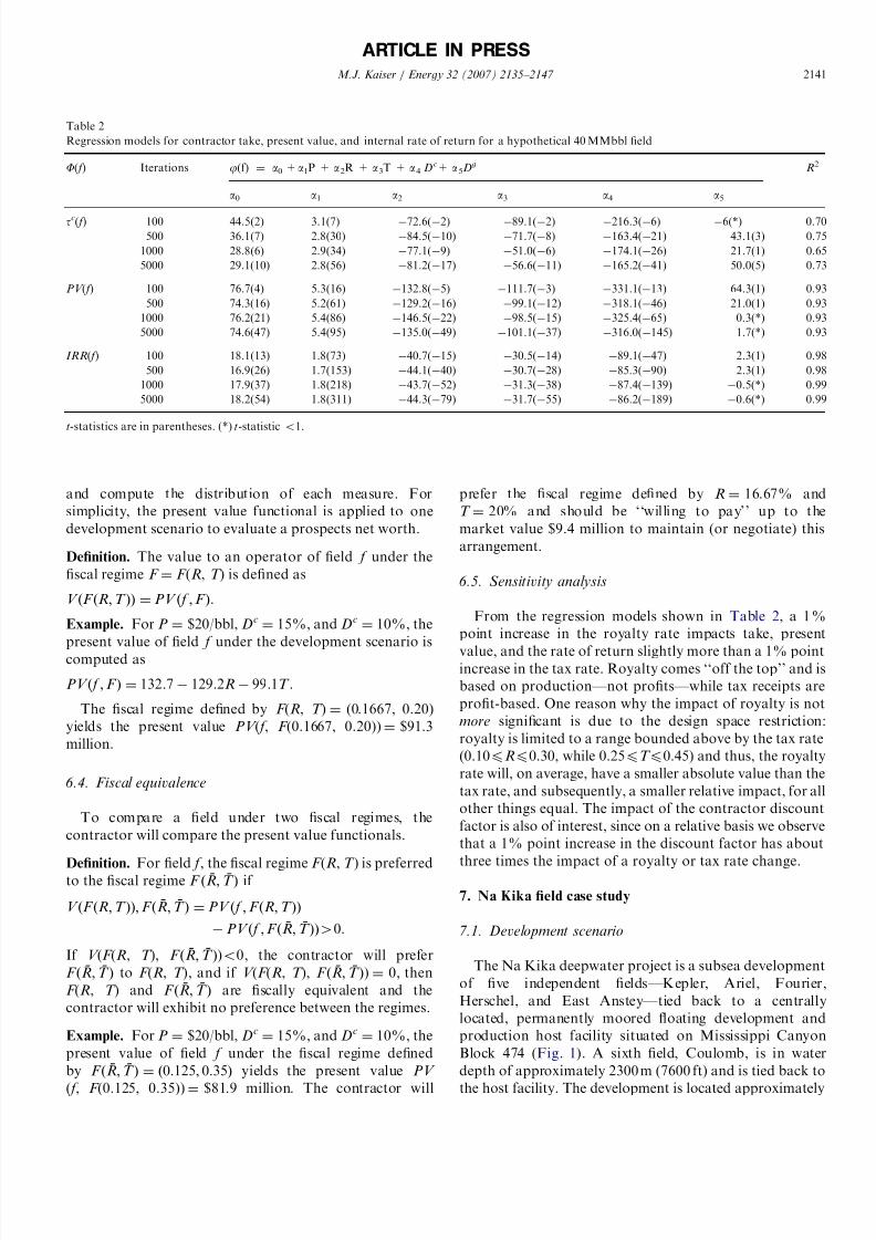
The model results are shown in Table 2 , and for the mostpart, the regression coefcients quickly stabilize withincreased sampling. The 500 data point simulation isconsidered representative:

t cð f ; F Þ ¼ 36:1 þ 2:8P o 84:5R 71:7T 163 :4D c

þ 43:1Dg; R2 ¼ 0:75,

PV ð f ; F Þ ¼ 74:3 þ 5:2P o 129 :2R 99:1T 318 :1D c

þ 21:0Dg

; R2

¼ 0:93,IRR ð f ; F Þ ¼ 16:9 þ 1:7P o 44:1R 30:7T 85:3D c

þ 2:3Dg; R2 ¼ 0:98.

All the coefcients have the expected signs and arestatistically signicant except the government discountfactor. Contractor take, present value, and the internal rateof return all increase with an increase in commodity price,and decline as royalty and tax rates increase. This behavioris expected, since an increase in the commodity price(holding all other factors xed) will increase the prot-ability of the eld. If the royalty and/or tax rate increases,the government will acquire a greater percentage of revenue which will decrease eld protability, and subse-quently, contractor take. As the contractor’s discountfactor is increased, the economics of eld developmentbecome progressively worse, and eventually, uneconomic.If the royalties and taxes collected by the government arediscounted at a higher rate, the contractor take andeconomic measures of the eld will increase.

6.3. Valuation strategy

To determine the impact of scal terms on projecteconomics, an operator will typically compare severaleconomic measures under different development scenarios,

ARTICLE IN PRESS

Table 1Projected production, capital expenditures, and operating expenditures fora hypothetical 40 MMbbl eld

Year Oilproduction(MMbbl)

CAPEX/I($M)

CAPEX/T($M)

OPEX($M)

1994 0 10 10 01995 0 5 8 0

1996 0 3 40 01997 4.500 0 25 11.51998 7.000 0 0 14.01999 5.600 0 0 12.62000 4.760 0 0 11.82001 4.046 0 0 11.02002 3.439 0 0 10.42003 2.923 0 0 9.92004 2.485 0 0 9.52005 2.087 0 0 9.12006 1.732 0 0 8.72007 1.427 0 0 8.42008 0 0 0 0

Total 40.000 18 83 117.0

Source: Johnston, Table 3 . [3,2].

M.J. Kaiser / Energy 32 (2007) 2135–2147 2140



and compute the distribution of each measure. Forsimplicity, the present value functional is applied to onedevelopment scenario to evaluate a prospects net worth.

Denition. The value to an operator of eld f under thescal regime F ¼ F (R , T ) is dened as

V ðF ðR ; T ÞÞ ¼ PV ð f ; F Þ.

Example. For P ¼ $20/bbl, Dc ¼ 15%, and Dc ¼ 10%, thepresent value of eld f under the development scenario iscomputed as

PV ð f ; F Þ ¼ 132 :7 129 :2R 99:1T .

The scal regime dened by F (R , T ) ¼ (0.1667, 0.20)yields the present value PV ( f , F (0.1667, 0.20)) ¼ $91.3million.

6.4. Fiscal equivalence

To compare a eld under two scal regimes, thecontractor will compare the present value functionals.

Denition. For eld f , the scal regime F (R , T ) is preferredto the scal regime F ð¯ R ; ¯ T Þ if

V ðF ðR ; T ÞÞ; F ð¯ R ; ¯ T Þ ¼ PV ð f ; F ðR ; T ÞÞ PV ð f ; F ð¯ R ; ¯ T ÞÞ4 0.

If V (F (R , T ), F ð¯ R ; ¯ T Þ)o 0, the contractor will preferF ð¯ R ; ¯ T Þ to F (R , T ), and if V (F (R , T ), F ð¯ R ; ¯ T Þ) ¼ 0, thenF (R , T ) and F ð¯ R ; ¯ T Þ are scally equivalent and thecontractor will exhibit no preference between the regimes.

Example. For P ¼ $20/bbl, Dc ¼ 15%, and Dc ¼ 10%, thepresent value of eld f under the scal regime denedby F ð¯ R ; ¯ T Þ ¼ ð0:125 ; 0:35Þ yields the present value PV ( f , F (0.125, 0.35)) ¼ $81.9 million. The contractor will

prefer the scal regime dened by R ¼ 16.67% andT ¼ 20% and should be ‘‘willing to pay’’ up to themarket value $9.4 million to maintain (or negotiate) thisarrangement.

6.5. Sensitivity analysis

From the regression models shown in Table 2 , a 1%point increase in the royalty rate impacts take, present

value, and the rate of return slightly more than a 1% pointincrease in the tax rate. Royalty comes ‘‘off the top’’ and isbased on production—not prots—while tax receipts areprot-based. One reason why the impact of royalty is notmore signicant is due to the design space restriction:royalty is limited to a range bounded above by the tax rate(0.10 p Rp 0.30, while 0.25 p T p 0.45) and thus, the royaltyrate will, on average, have a smaller absolute value than thetax rate, and subsequently, a smaller relative impact, for allother things equal. The impact of the contractor discountfactor is also of interest, since on a relative basis we observethat a 1% point increase in the discount factor has aboutthree times the impact of a royalty or tax rate change.

7. Na Kika eld case study

7.1. Development scenario

The Na Kika deepwater project is a subsea developmentof ve independent elds—Kepler, Ariel, Fourier,Herschel, and East Anstey—tied back to a centrallylocated, permanently moored oating development andproduction host facility situated on Mississippi CanyonBlock 474 ( Fig. 1 ). A sixth eld, Coulomb, is in waterdepth of approximately 2300 m (7600 ft) and is tied back tothe host facility. The development is located approximately

ARTICLE IN PRESS

Table 2Regression models for contractor take, present value, and internal rate of return for a hypothetical 40 MMbbl eld

F ( f ) Iterations j (f) ¼ a0 + a1P + a 2R + a 3T + a 4 D c+ a 5Dg R 2

a0 a1 a2 a3 a4 a5

t c( f ) 100 44.5(2) 3.1(7) 72.6( 2) 89.1( 2) 216.3( 6) 6(*) 0.70500 36.1(7) 2.8(30) 84.5( 10) 71.7( 8) 163.4( 21) 43.1(3) 0.75

1000 28.8(6) 2.9(34) 77.1( 9) 51.0( 6) 174.1( 26) 21.7(1) 0.655000 29.1(10) 2.8(56) 81.2( 17) 56.6( 11) 165.2( 41) 50.0(5) 0.73

PV ( f ) 100 76.7(4) 5.3(16) 132.8( 5) 111.7( 3) 331.1( 13) 64.3(1) 0.93500 74.3(16) 5.2(61) 129.2( 16) 99.1( 12) 318.1( 46) 21.0(1) 0.93

1000 76.2(21) 5.4(86) 146.5( 22) 98.5( 15) 325.4( 65) 0.3(*) 0.935000 74.6(47) 5.4(95) 135.0( 49) 101.1( 37) 316.0( 145) 1.7(*) 0.93

IRR ( f ) 100 18.1(13) 1.8(73) 40.7( 15) 30.5( 14) 89.1( 47) 2.3(1) 0.98500 16.9(26) 1.7(153) 44.1( 40) 30.7( 28) 85.3( 90) 2.3(1) 0.98

1000 17.9(37) 1.8(218) 43.7( 52) 31.3( 38) 87.4( 139) 0.5(*) 0.995000 18.2(54) 1.8(311) 44.3( 79) 31.7( 55) 86.2( 189) 0.6(*) 0.99

t-statistics are in parentheses. (*) t-statistic o 1.

M.J. Kaiser / Energy 32 (2007) 2135–2147 2141



140 miles southeast of New Orleans in water depthsranging from 1800 m (5800ft) to 2100 m (7000ft).

Shell and BP each hold a 50% interest in the host facilityand the Kepler, Ariel, Fourier, and Herschel elds. In EastAnstey, Shell has a 37.5% interest with BP holding theremaining 62.5%, and in the Coulomb eld, Shell has a

100% interest.The host is a semi-submersible-shaped hull with topsidefacilities for uid processing and pipelines for oil and gasexport to shore ( Fig. 2 ). The elds produce from 12 satellitesubsea wells equipped to handle 425 MMcf/day of gas,110,000 bbl/day of oil, and 7000 bbl/day of water. TheKepler, Ariel, and Herschel elds are primarily oil, whilethe Fourier and East Anstey elds are primarily gas. The

API gravity of the elds range from 25 1 (Herschel) to 29 1(Fourier). The rst phase of production from 10 wells inKepler, Ariel, Fourier, East Anstey, and Herschel wentonstream 4Q 2003. Coulomb began production in 2004from two subsea wells.

The development scenario for Na Kika is based on an

estimated gross ultimate recovery of 300 MMBOE. Provedreserves are currently estimated at 189 MMbbl of oiland 728 Bcf of gas. The cash ow projection is shown inTable 3 . Total project cost is approximately $1.26 billion,excluding lease costs of $20 million. Approximately 50% of the costs are associated with the fabrication and installa-tion of the host facility and pipeline, 25% of the costs areassociated with the fabrication and installation of the

ARTICLE IN PRESS

Fig. 2. The Na Kika Host Platform and Subsea Well Conguration. Source : Shell.

Fig. 1. The Na Kika Field Development. Source : Shell.

M.J. Kaiser / Energy 32 (2007) 2135–2147 2142



subsea components, and 25% are associated with thedrilling and completion of the wells. The life cycle capitalexpenditures is estimated as $3.73/bbl with operating costestimated at $1.20/bbl. OPEX is forecast to increasesteadily from less than $1/bbl early in the production cycleto over $8/bbl near the end of the life of the eld.

7.2. Deepwater royalty relief

For leases acquired between November 28, 1995 andNovember 28, 2000, the Outer Continental Shelf Deep-

water Royalty Relief Act (DWRRA; 43 USC. Section1337) provided economic incentives for operators todevelop elds in water depths greater than 200 m (656 ft).The incentives provide for the automatic suspension of royalty payments on the initial 17.5 MMBOE producedfrom a eld in 200–400 m (656–1312 ft) of water,52.5 MMBOE for a eld in 400–800 m (1312–2624 ft) of water, and 87.5MMBOE for a eld in greater than 800m(2624ft) of water [26]. The DWRRA expired on November28, 2000, but leases acquired during the time royalty relief was active retain the incentives until their expiration.Reduction of royalty payments is also available through anapplication process for deepwater elds leased prior to theDWRRA but which had not yet gone on production.Provisions effective in 2001 are specied on a lease basis,and are subject to change with each lease sale as economicconditions warrant.

If Qt denotes the annual hydrocarbon production fromeld f in year t, d ( f ) the (average) water depth of the eld,and Q( f ) the volume of production for which royalty issuspended, then deepwater royalty rates are determined asfollows:

R ¼

0; if PtQ t p Qð f Þ;

16:67% ; if

Pt

Q t4 Qð f Þ:8><>:

If the lease on which the eld is located was acquiredbetween November 28, 1995 and November 28, 2000, then

Qð f Þ ¼

17:5 MMBOE ; if 200m p d ð f Þp 399m ;52:5 MMBOE ; if 400m p d ð f Þp 799m ;87:5 MMBOE ; if dðf ÞX 800m

8><>:

For lease sales held after November 28, 2000, the waterdepth categories and value of Q( f ) is specic to the leasesale.

7.3. Regression model results

The design space for four models are shown in Table 4 .In Model I, the system parameters are selected uniformlyfrom each design interval, and in Model II, the designintervals are more narrowly dened and the hydrocarbonprices assumed Lognormally distributed. Model III em-ploys the same parameter intervals as in Model II but theoil and gas price is assumed to vary over each year of theproduction cycle; i.e., P ot LN(25, 5), P gt LN(3.5, 1.5) fort ¼ 1,y , 12. In Model IV, the Model III parameters areapplied with an annual tax rate selected from a triangulardistribution; i.e., T t TR(0.38, 0.44, 0.50) for t ¼ 1,y , 12.

The results of the regression models for t cð f ; F Þ, PV ( f , F )and IRR ( f , F ) are shown in Table 5 . The model coefcientshave the expected signs, the ts are robust, and all thecoefcients—except the government discount factor—arehighly signicant. For any value of ( P o, P g, R , Q, T , Dc, Dg)within the design space, the regression model can be usedto evaluate and compare parameter selections. Note thatthe design space includes the variables P g, gas price, and Q ,royalty relief threshold, specic to the Na Kika eld.

In Model I, the results of the meta-model yield

t cð f Þ ¼ 80:0 þ 0:2P o þ 0:5P g 53:0R þ 0:04Q 79:1T

84:3D c þ 86:2Dg; R2 ¼ 0:99;

ARTICLE IN PRESS

Table 3Projected production, capital expenditures, and operating expenditures for the Na Kika eld development

Year Oil production(bbl/day)

Gas production(MMcf/day)

CAPEX/T ($M) CAPEX/I ($M) OPEX ($M)

2001 0.0 0.0 52.83 0.00 0.002002 0.0 0.0 350.13 19.24 0.002003 100,000.0 325.0 475.33 263.98 5.662004 95,177.5 312.0 0.00 0.00 25.302005 95,177.5 312.0 0.00 0.00 30.092006 82,002.8 304.2 0.00 0.00 30.092007 55,538.0 235.5 0.00 0.00 30.092008 37,514.4 171.9 0.00 0.00 30.092009 25,279.5 125.2 0.00 0.00 37.282010 16,683.1 91.5 0.00 0.00 37.282011 11,694.0 66.8 0.00 0.00 37.282012 0.0 48.8 0.00 0.00 106.47

Total 878.29 283.22 369.65

Source : MMS.

M.J. Kaiser / Energy 32 (2007) 2135–2147 2143



PV ð f Þ ¼ 10460 :7 þ 38:2P o þ 131 :5P g 1259 :8R þ 1:1Q

1856 :1T 3699 :4 þ 79:8; R2 ¼ 0:97,

IRR ð f Þ ¼ 63:4 þ 2:6P o þ 8:6P g 58:9R þ 0:1Q 126 :2T

131 :5D c þ 2:2D g; R2 ¼ 0:99.

A quick glance at the regression coefcients indicates thecharacteristics of royalty relief. First, the absolute magni-tude of the tax coefcients exceeds the royalty rate. This isnot entirely unexpected since a royalty suspension has beengranted on the rst Q( f ) MMBOE production therebydampening its impact. Under royalty relief, the governmentforegoes royalty for a period of time, but its tax collectionwill increase (since the operators revenue will increase withsuspended royalties).

The contractor and government discount factors areapproximately equal in the take computation, but asignicant difference exists in the present value and rateof return measures. If Dc and Dg are required to satisfy

D c ¼ Dg ¼ D , the new model coefcients for D is nearlythe same as D c and the rest of the model coefcients do notchange appreciably.

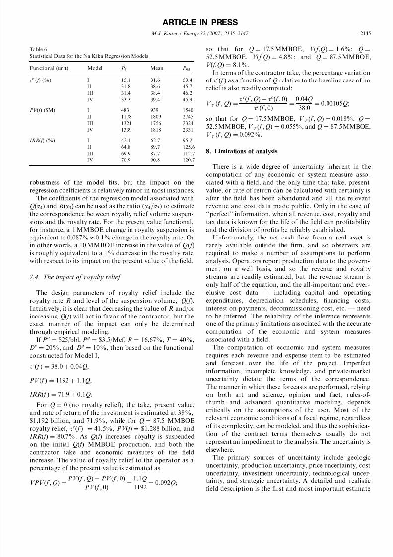
In Model II, the hydrocarbon prices are assumedLognormally distributed and the design intervals are morenarrowly dened. The impact of these changes to theregression models is shown in Table 5 . The mean, P

5, and

P 95 estimates 5 of the computed measures is shown in Table6. These values bound the expected range of each measurefor the design space and model specication. Observe thatas the design specication becomes more narrowly denedthe range dened by P 95 – P 5 generally shrinks, while thevariability introduced through P ot and P gt do not noticeablyaffect the range.

The inclusion of structural variability in Models IIIand IV, where the hydrocarbon prices and tax rates arenow assumed to vary annually, negatively impacts the

ARTICLE IN PRESS

Table 5The impact of royalty relief on contractor take, present value, and internal rate of return for the Na Kika eld development

F ( f ) Model j (f)¼a 0+ a 1P+ a 2P g+ a 3R+ a 4Q+ a 5T+ a 6D+ a 7D g R2

a 0 a 1 a 2 a 3 a 4 a 5 a 6 a 7

t ( f ) I 80.0(161) 0.2(18) 0.5(13) 53.0( 50) 0.04(42) 79.1( 112) 84.3( 198) 86.2(78) 0.99II 86.7(369) 0.2(26) 0.1(21) 54.1( 51) 0.04(121) 77.4( 243) 108.6( 337) 107.9(164) 0.99III 86.8(123) 0.1(4) 0.1(2) 53.3( 21) 0.03(50) 78.6( 99) 107.9( 145) 107.0(70) 0.98IV 86.7(30) 0.1(1) 0.1(*) 54.6( 12) 0.04(30) 76.0(12) 108.9( 81) 106.8(40) 0.95

PV ( f ) I 1460.7(33) 38.2(40) 131.5(42) 1259.8(79) 1.1(12) 1856.1( 30) 3699.4( 99) 79.8(1) 0.97II 2113.6(29) 56.9(98) 232.0(119) 2200.6( 7) 1.8(17) 3404.8( 35) 8294.5( 83) 27.6(*) 0.98III 2252.5(12) 52.6(12) 226.5(14) 1957.1( 3) 1.2(6) 3414.2( 17) 8086.6( 42) 609.8(2) 0.84IV 2088.8(4) 74.2(14) 212.9(13) 3285.9( 4) 2.2(9) 3632.6( 3) 8407.1(34) 212.1(*) 0.75

IRR ( f ) I 63.4(54) 2.6(145) 8.6(103) 58.9( 24) 0.1(49) 126.2( 76) 131.5( 131) 2.2(1) 0.99

II 72.9(40) 2.8(185) 5.6(196) 68.4( 8) 0.2(50) 150.0( 61) 171.5( 65) 2.2(*) 0.99III 82.8(6) 2.9(9) 8.4(7) 68.5( 1) 0.1(7) 167.2( 10) 160.0( 11) 1.6(*) 0.44IV 83.9(2) 3.4(8) 7.71(6) 169.1 ( 3) 0.2(9) 152.1( 2) 186.8( 9) 19.8( 2) 0.34

t-statistics are in parentheses, (*) t-statistic o 1.

Table 4The design space of the Na Kika system parameters

Parameter (unit) Model I Model II Model III Model IV

P o ($/bbl) U(20, 30) a LN(25, 5) b LN(25, 5) c LN(25, 5) c

P g ($/Mcf) U(2, 5) LN(3.5, 1.5) LN(3.5, 1.5) c LN(3.5, 1.5) c

R (%) U(0.10, 0.20) U(0.15, 0.18) U(0.15, 0.18) U(0.15, 0.18)Q (MMBOE) U(0, 100) U(0, 100) U(0, 100) U(0, 100)T (%) U(0.35, 0.50) U(0.40, 0.50) U(0.40, 0.50) TR(0.38, 0.44, 0.50) d

D c (%) U(0.15, 0.40) U(0.05, 0.15) U(0.05, 0.15) U(0.05, 0.15)D g (%) U(0.05, 0.15) U(0.00, 0.05) U(0.00, 0.05) U(0.00, 0.05)

a U( a , b) denotes a Uniform probability distribution with endpoints ( a , b).b LN( c, d ) represents a Lognormal probability distribution with mean c and standard deviation d .cP o and P g are assumed to vary on an annual basis; i.e., P o ¼ P t

o LN(25, 5) and P g ¼ P tg LN(3.5, 1.5) for t ¼ 1,y ,12.

d TR( e, f , g) represents a Triangular probability distribution with minimum e, most likely f , and maximum g. T is assumed to vary on an annual basis;i.e., T ¼ T t TR(0.38, 0.44, 0.50) for t ¼ 1, y , 12.

5The P 5 and P 95 measures indicate that 5% of the time the estimatedvalue is expected to be less than P 5 or greater than P 95 .

M.J. Kaiser / Energy 32 (2007) 2135–2147 2144



robustness of the model ts, but the impact on theregression coefcients is relatively minor in most instances.

The coefcients of the regression model associated withQða 4Þ and Rða 3Þ can be used as the ratio ða 4=a3Þ to estimatethe correspondence between royalty relief volume suspen-sions and the royalty rate. For the present value functional,for instance, a 1 MMBOE change in royalty suspension isequivalent to 0.087% E 0.1% change in the royalty rate. Orin other words, a 10 MMBOE increase in the value of Q ( f )is roughly equivalent to a 1% decrease in the royalty ratewith respect to its impact on the present value of the eld.

7.4. The impact of royalty relief

The design parameters of royalty relief include theroyalty rate R and level of the suspension volume, Q( f ).Intuitively, it is clear that decreasing the value of R and/orincreasing Q( f ) will act in favor of the contractor, but theexact manner of the impact can only be determinedthrough empirical modeling.

If P o ¼ $25/bbl, P g ¼ $3.5/Mcf, R ¼ 16.67%, T ¼ 40%,D c ¼ 20%, and Dg ¼ 10%, then based on the functionalconstructed for Model I,

t cð f Þ ¼ 38:0 þ 0:04Q ,

PV ð f Þ ¼ 1192 þ 1:1Q ,

IRR ð f Þ ¼ 71:9 þ 0:1Q .

For Q ¼ 0 (no royalty relief), the take, present value,and rate of return of the investment is estimated at 38%,$1.192 billion, and 71.9%, while for Q ¼ 87.5 MMBOEroyalty relief, t cð f Þ ¼ 41.5%, PV ( f ) ¼ $1.288 billion, andIRR ( f ) ¼ 80.7%. As Q( f ) increases, royalty is suspendedon the initial Q( f ) MMBOE production, and both thecontractor take and economic measures of the eldincrease. The value of royalty relief to the operator as apercentage of the present value is estimated as

VPV ð f ; QÞ ¼ PV ð f ; QÞ PV ð f ; 0Þ

PV ð f ; 0Þ ¼

1:1Q

1192 ¼ 0:092 Q ;

so that for Q ¼ 17.5 MMBOE, V ( f ,Q) ¼ 1.6%; Q ¼52.5 MMBOE, V ( f ,Q ) ¼ 4.8%; and Q ¼ 87.5 MMBOE,V ( f ,Q) ¼ 8.1%.

In terms of the contractor take, the percentage variationof t cð f Þ as a function of Q relative to the baseline case of norelief is also readily computed:

V t c ð f ; QÞ ¼ t cð f ; QÞ t cð f ; 0Þt cð f ; 0Þ

¼ 0:04Q38:0

¼ 0:00105 Q ;

so that for Q ¼ 17.5MMBOE, V t c ð f ; QÞ ¼ 0.018%; Q ¼52.5MMBOE, V t c ð f ; QÞ ¼ 0.055%; and Q ¼ 87.5MMBOE,V t c ð f ; QÞ ¼ 0.092%.

8. Limitations of analysis

There is a wide degree of uncertainty inherent in thecomputation of any economic or system measure asso-ciated with a eld, and the only time that take, presentvalue, or rate of return can be calculated with certainty isafter the eld has been abandoned and all the relevantrevenue and cost data made public. Only in the case of ‘‘perfect’’ information, when all revenue, cost, royalty andtax data is known for the life of the eld can protabilityand the division of prots be reliably established.

Unfortunately, the net cash ow from a real asset israrely available outside the rm, and so observers arerequired to make a number of assumptions to performanalysis. Operators report production data to the govern-ment on a well basis, and so the revenue and royaltystreams are readily estimated, but the revenue stream isonly half of the equation, and the all-important and ever-

elusive cost data — including capital and operatingexpenditures, depreciation schedules, nancing costs,interest on payments, decommissioning cost, etc. — needto be inferred. The reliability of the inference representsone of the primary limitations associated with the accuratecomputation of the economic and system measuresassociated with a eld.

The computation of economic and system measuresrequires each revenue and expense item to be estimatedand forecast over the life of the project. Imperfectinformation, incomplete knowledge, and private/marketuncertainty dictate the terms of the correspondence.The manner in which these forecasts are performed, relyingon both art and science, opinion and fact, rules-of-thumb and advanced quantitative modeling, dependscritically on the assumptions of the user. Most of therelevant economic conditions of a scal regime, regardlessof its complexity, can be modeled, and thus the sophistica-tion of the contract terms themselves usually do notrepresent an impediment to the analysis. The uncertainty iselsewhere.

The primary sources of uncertainty include geologicuncertainty, production uncertainty, price uncertainty, costuncertainty, investment uncertainty, technological uncer-tainty, and strategic uncertainty. A detailed and realisticeld description is the rst and most important estimate

ARTICLE IN PRESS

Table 6Statistical Data for the Na Kika Regression Models

Functional (unit) Model P 5 Mean P 95

t c ( f ) (%) I 15.1 31.6 53.4II 31.8 38.6 45.7III 31.4 38.4 46.2IV 33.3 39.4 45.9

PV ( f ) ($M) I 483 939 1540II 1178 1809 2745III 1321 1756 2324IV 1339 1818 2331

IRR ( f ) (%) I 42.1 62.7 95.2II 64.8 89.7 125.6III 69.9 87.7 112.7IV 70.9 90.8 120.7

M.J. Kaiser / Energy 32 (2007) 2135–2147 2145



that must be made. The size, shape, productive zones, faultblocks, drive mechanisms, etc. of the reservoir must beestimated with as much accuracy as possible since theydetermine the capacity of the structure and the requirednumber and location of wells. Estimates of productionrates are based on geologic conditions at the reservoir level,

decline curve analysis or similar techniques. Forecastproduction is only used as a guideline, however, sinceinvestment activity can dramatically alter the form of theproduction curve as well as recoverable reserves. Hydro-carbon price, development cost, technological improve-ments, and demand–supply relations impact the revenue of a lease and investment planning. Strategic objectives of acorporation are generally unobservable, nonquantiable,and can vary dramatically over time.

9. Conclusions

To understand the economic and system measuresassociated with a royalty/tax scal regime a meta-modelwas developed. In the meta-evaluation procedure, a cashow model specic to a given scal regime is used togenerate meta data that describes the inuence of varioussystem variables. Meta-modeling is not a new idea,but as applied to scal system analysis and contractvaluation, is both new and novel, as it provides insight intothe factors that inuence system metrics and their relativeimpact.

A constructive approach to scal system analysis wasdeveloped to determine the manner in which private andmarket uncertainty impact take and the economic measures

associated with a eld. Functional relations were developedby computing the component measures for parametervectors selected within a given design space. The relativeimpact of the parameters and the manner in which thevariables are correlated was also established in a generalmanner. The methodology was illustrated on a hypothe-tical oil eld and a case study for the deepwater Na Kikadevelopment was considered. Representative results on theimpact of royalty relief on the eld economics of Na Kikawas presented.

Acknowledgments

The advice, patience, and critical comments of RadfordSchantz, Stephanie Gambino, and Kristen Strellec aregratefully acknowledged. Radford Schantz suggested theinitial formulation of the problem considered in this paper,and special thanks also goes to Thierno Sow of the MMSfor generating the cash ow parameters for Na Kika. Thispaper was prepared on behalf of the U.S. Department of the Interior, Minerals Management Service, Gulf of Mexico OCS region, and has not been technically reviewedby the MMS. The opinions, ndings, conclusions, orrecommendations expressed in this paper are those of the authors, and do not necessarily reect the viewsof the Minerals Management Service. Funding for this

research was provided through the U.S. Department of theInterior and the Coastal Marine Institute, Louisiana StateUniversity.

References

[1] Anderson OL. Royalty valuation: Should royalty obligations bedetermined intrinsically, theoretically, or realistically. Natural Re-sources Law Journal 1998;37:611.

[2] Gerwich Jr BC. Construction of marine and offshore structures. BocaRaton, FL: CRC Press; 2000.

[3] Johnston D. International petroleum scal systems and productionsharing contracts. Tulsa, OK: PennWell Books; 1994.

[4] Gallun RA, Wright CJ, Nichols LM, Stevenson JW. Fundamentalsof oil & gas accounting. 4th ed. Tulsa, OK: PennWell Books; 2001.

[5] Thompson RS, Wright JD. Oil property evaluation. Golden, CO:Thompson-Wright Associates; 1984.

[6] Van Meurs APH. Petroleum economics and offshore mininglegislation. Amsterdam: Elsevier Publishing Company; 1971.

[7] Boudreaux DO, Ward DR, Boudreaux P, Ward SP. An inquiry into

the capital budgeting process and analytical procedures utilized byrms in the oil and gas extraction industry. Pet Accounting FinancialManage J 1991;24–34.

[8] Pohlman PA, Santiago ES, Market FL. Cash ow estimationpractices of large rms. Financial Manag 1987; Spring: 46–51.

[9] Mian MA. Project economics and decision analysis. vol. 1:deterministic models. Tulsa, OK: PennWell Books; 2002.

[10] Dougherty EL. Guidelines for proper application of four commonlyused investment criteria. In: SPE paper 13770, SPE hydrocarboneconomics and evaluation symposium, Dallas, TX; 1985. p. 101–15.

[11] Seba RD. The only investment selection criterion you will ever need.In: SPE paper 16310, SPE hydrocarbon economics and evaluationsymposium, Dallas, TX; March 2–3, 1987. p. 173-180.

[12] Johnston D. Current developments in production sharing contractsand international concerns: retrospective government take — not a

perfect statistic. Petroleum Accounting and Financial ManagementJournal 2002;21(2):101–8.

[13] Rapp WJ, Litvak, BL, Kokolis, GP, Wang B. Utilizing discountedgovernment take analysis for comparison of international oil and gasE&P scal regimes. SPE Paper 52958 , SPE hydrocarbon economicsand evaluation symposium, Dallas, TX; March 20–23, 1999.

[14] Smith D. True government take (TGT): a measurement of scalterms. SPE Paper 16308 , SPE hydrocarbon economics and evalua-tion symposium, Dallas, TX; March 2–3, 1987.

[15] Rutledge I, Wright P. Protability and taxation: Analyzing thedistribution of rewards between company and country. Energy Policy1998;26.

[16] Johnston D. Global petroleum scal systems compared by contractortake. Oil and Gas Journal 1994;92(50):47–50.

[17] Kemp A. Petroleum rent collection around the world, Halifax, Nora

Sistia: The Institute for Research on Public Policy; 1987.[18] Meurs APV, Seck A. Governments cut takes to compete as world

acreage demand falls. Oil and Gas Journal 1995;24:78–82.[19] Meurs APV, Seck A. Government takes decline as nations diversify

terms to attract investment. Oil Gas 1997;26:35–40.[20] Allen FH, Seba RD. Economics of worldwide petroleum production.

Tulsa, OK: Oil and Gas Consultants International (OGCI), Inc.;1993.

[21] Ehrhardt MC. The search for value: measuring the company’s cost of capital. Boston, MA: Harvard Business School Press; 1994.

[22] Ofce of Management and Budget, United States Government.Guidelines and discount rates for benet-cost analysis of federalprograms. OMB Circular 1-94 (revised), October 1992.

[23] Wood DA. Economic performance of rate of return driveninternational petroleum production contracts. Pet AccountingFinancial Manage 1993;13(2):84–102.

ARTICLE IN PRESS

M.J. Kaiser / Energy 32 (2007) 2135–2147 2146



[24] Wood DA. Evaluation of economic performance of internationalexploration contracts, Parts 1 and 2. Oil and Gas Journal 1990;88(44,45):1990.

[25] Smith D. Methodologies for comparing scal systems. Pet Account-ing Financial Manage 1993;13(2):76–83.

[26] Baud RD, et al. Deepwater Gulf of Mexico 2002: America’sexpanding frontier. OCS report MMS 2002-021, U.S. Departmentof the Interior, Minerals Management Service, Gulf of MexicoOCS Region, Ofce of Resource Evaluation, New Orleans;April 2002.

ARTICLE IN PRESS

M.J. Kaiser / Energy 32 (2007) 2135–2147 2147

fiscal system analysis concessionary systems

Documents