fitting the cusp catastrophe in r: a cusp package primer · fitting the cusp catastrophe in r: a...

JSS Journal of Statistical SoftwareNovember 2009, Volume 32, Issue 8. http://www.jstatsoft.org/

Fitting the Cusp Catastrophe in R: A cusp Package

Primer

Raoul P. P. P. GrasmanUniversiteit van Amsterdam

Han L. J. van der MaasUniversiteit van Amsterdam

Eric-Jan WagenmakersUniversiteit van Amsterdam

Abstract

Of the seven elementary catastrophes in catastrophe theory, the “cusp” model is themost widely applied. Most applications are however qualitative. Quantitative techniquesfor catastrophe modeling have been developed, but so far the limited availability of flexiblesoftware has hindered quantitative assessment. We present a package that implements andextends the method of Cobb (Cobb and Watson 1980; Cobb, Koppstein, and Chen 1983),and makes it easy to quantitatively fit and compare different cusp catastrophe modelsin a statistically principled way. After a short introduction to the cusp catastrophe, wedemonstrate the package with two instructive examples.

Keywords: catastrophe theory, cusp, modeling.

Catastrophe theory studies qualitative changes in behavior of systems under smooth gradualchanges of control factors that determine their behavioral state. In doing so, catastrophetheory has been able to explain for example, how sudden abrupt changes in behavior can resultfrom minute changes in the controlling factors, and why such changes occur at different controlfactor configurations depending on the past states of the system. Specifically, catastrophetheory predicts all the types of qualitative behavioral changes that can occur in the class ofso called gradient systems, under influence of gradual changes in controlling factors (Postonand Stewart 1996).

Catastrophe theory was popularized in the 1970’s (Thom 1973; Thom and Fowler 1975;Gilmore 1993), and was suggested as a strategy for modeling in various disciplines, likephysics, biology, psychology, and economics, by Zeeman (1971)—as cited in Stewart andPeregoy (1983), Zeeman (1973), Zeeman (1974), Isnard and Zeeman (1976), and Poston andStewart (1996). Although catastrophe theory is well established and applied in the physicalsciences, its applications in the biological sciences, and especially in the social and behavioralsciences, has been criticized (Sussmann and Zahler 1978; Rosser 2007). Applications in thelatter fields range from modeling of exchange market crashes in economics (Zeeman 1974), to

http://www.jstatsoft.org/

2 cusp: Fitting the Cusp Catastrophe in R

perception of bistable figures (Stewart and Peregoy 1983; Ta’eed, Ta’eed, and Wright 1988;Furstenau 2006) in psychology. The major points of criticism concerned the overly qualitativemethodology used in applications in the latter sciences, as well as the ad hoc nature of thechoice of variables used as control variables. The first of these seems to stem from the factthat catastrophe theory concerned deterministic dynamical systems, whereas applications inthese sciences concern data that are more appropriately considered stochastic. For an histor-ical summary of the developments and critiques of catastrophe theory we refer the reader toRosser (2007).

Stochastic formulations of catastrophe theory have been found, and statistical methods havebeen developed that allow quantitative comparison of catastrophe models with data (Cobband Ragade 1978; Cobb and Watson 1980; Cobb 1981; Cobb et al. 1983; Guastello 1982; Oliva,Desarbo, Day, and Jedidi 1987; Lange, Oliva, and McDade 2000; Wagenmakers, Molenaar,Grasman, Hartelman, and van der Maas 2005a; Guastello 1992). Of these methods, themaximum likelihood approach of Cobb and Watson (1980); Cobb et al. (1983) is arguablymost appealing for reasons that we discuss in the Appendix A.

In this paper we present an add-on package for the statistical computing environment R(R Development Core Team 2009) which implements the method of (Cobb et al. 1983), andextends it in a number of ways. In particular, the approach of Oliva et al. (1987) is adopted toallow for a behavioral variable that is embedded in multivariate response space. Furthermore,the implementation incorporates many of the suggestions of Hartelman (1997), and indeedintends to succeed and update the cuspfit FORTRAN program of that author. The packageis available from the Comprehensive R Archive Network at http://CRAN.R-project.org/package=cusp.

1. Cusp catastrophe

Consider a (deterministic) dynamical system that obeys equations of motion of the form

∂y

∂t= −∂V (y; c)

∂y, y ∈ Rk, c ∈ Rp. (1)

In this equation y(t) represents the system’s state variable(s), and c represents one or multiple(control) parameter(s) who’s value(s) determine the specific structure of the system. If thesystem state y is at a point where ∂V (y; c)/dx = 0 the system is in equilibrium. If thesystem is at a non-equilibrium point, the system will move towards an equilibrium pointwhere the function V (y; c) acquires a minimum with respect to y. These equilibrium pointsare stable equilibrium points because the system will return to such a point after a smallperturbation to the system’s state. Equilibrium points that correspond to maxima of V (y; c)are unstable equilibrium points because a perturbation of the system’s state will cause thesystem to move away from the equilibrium point towards a stable equilibrium point. Inthe physical world no system is fully isolated and there are always forces impinging on asystem. It is therefore highly unlikely to encounter a system in an unstable equilibriumstate. Equilibrium points that correspond neither to maxima nor to minima of V (y; c), atwhich the Hessian matrix (∂2V (y)/∂yi∂yj) has eigenvalues equal to zero, are called degenerateequilibrium points, and these are the points at which a system can give rise to unexpectedbifurcations in its equilibrium states when the control variables of the system are changed.

http://CRAN.R-project.org/package=cusp

http://CRAN.R-project.org/package=cusp

Journal of Statistical Software 3

1.1. Canonical form

Catastrophe theory (Thom 1973; Thom and Fowler 1975; Gilmore 1993; Poston and Stewart1996) classifies the behavior of deterministic dynamical systems in the neighborhood of de-generate critical points of the potential function V (y; c). One of the remarkable findings ofcatastrophe theory is its discovery that degenerate equilibrium points of systems of the formdescribed above, which have an arbitrary numbers of state variables and are controlled by nomore than four control variables, can be characterized by a set of only seven canonical forms,or “universal unfoldings”, in only one or two canonical state variables. These universal un-foldings are called the “elementary catastrophes”. The canonical state variables are obtainedby smooth transformations of the original state variables. The elementary catastrophes con-stitute the different families of catastrophe models.

In the biological and behavioral sciences, the so-called cusp catastrophe model has beenapplied most frequently, as it is the simplest of catastrophe models that exhibits discontinuoustransitions in equilibrium states as control parameters are varied. The canonical form of thepotential function for the cusp catastrophe is

−V (y;α, β) = αy +12β y2 − 1

4y4. (2)

Its equilibrium points, as a function of the control parameters α and β, are solutions to theequation

α+ β y − y3 = 0. (3)

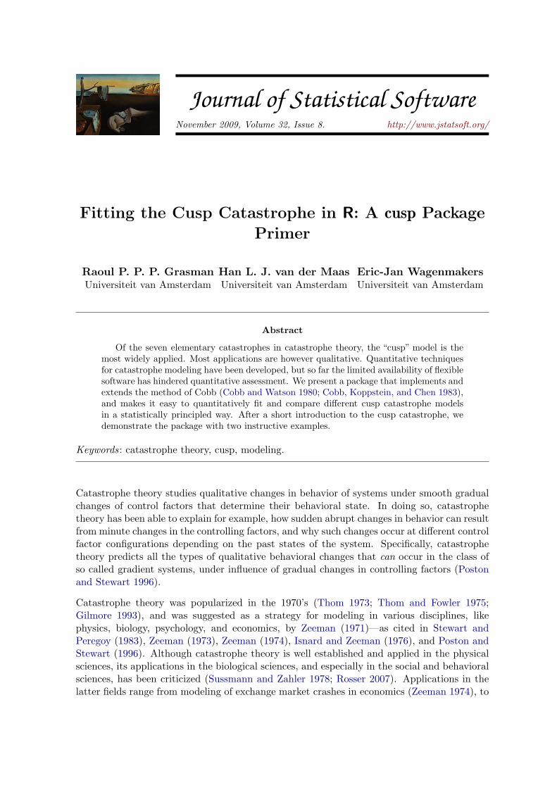
This equation has one solution if δ = 27α− 4β3, which is known as Cardan’s discriminant, isgreater than zero, and has three solutions if δ < 0. These solutions are depicted in Figure 1as a two dimensional surface living in three dimensional space, the floor of which is the twodimensional (α, β) coordinate system called the “control plane”. The set of values of α and βfor which δ = 0 demarcates the bifurcation set, the cross hatched cusp shaped region on thefloor in Figure 1. From a regression perspective, the cusp equilibrium surface may be conceivedof as response surface, the height of which predicts the value of the dependent variable y giventhe values of the control variables. This response surface has the peculiar property however,that for some values of the control variables α and β the surface predicts two possible valuesinstead of one. In addition, this response surface has the unusual characteristic that it “anti-predicts” an intermediate value for these values of the control variables—that is, the surfacepredicts that certain state values, viz. unstable equilibrium states, should not occur (Cobb1980). As indicated, the dependent variable y is not necessarily an observed quantity thatcharacterizes the system under study, but is in fact a canonical variable that in generaldepends on a number of actually measurable dependent variables. Similarly, the controlcoordinates α and β represent canonical coordinates that are dependent on actual measuredor controlled independent variables. The α coordinate is called the “normal” or “asymmetry”coordinate, while the β coordinate is called the“bifurcation”or“splitting”coordinate (Stewartand Peregoy 1983).

1.2. Cusp catastrophe as a model

In evaluating the cusp as a model for data there are two complementary approaches. Thefirst approach evaluates whether certain qualitative phenomena occur in the system underconsideration. In the second approach, a parameterized cusp is fitted to the data.


alpha

beta

equilibrium states

Cusp Equilibrium Surface

Figure 1: Cusp surface.

Gilmore (1993) derived a number of qualitative behavioral characteristics of the cusp model;the so-called catastrophe flags. Among the more prominent are sudden jumps in the value ofthe (canonical) state variables; hysteresis—i.e., memory for the path through the phase spaceof the system; and multi-modality—i.e., the simultaneously presence of multiple preferredstates. Verification of the presence of these flags constitute one important stage in gatheringevidence for the presence of a cusp catastrophe in the system under scrutiny. For extensivediscussions of these qualitative flags we refer to Gilmore (1993)—see also Stewart and Peregoy(1983), van der Maas and Molenaar (1992), and van der Maas, Kolstein, and van der Pligt(2003).

Most applications of catastrophe theory in general, and the cusp catastrophe in particular,have focused entirely on this qualitative verification. An alternative approach is constitutedby a quantitative evaluation of an actual match between a cusp catastrophe model and thedata using statistical fitting procedures. This is indispensable for sound verification that a


−30 −20 −10 0 10 20 30

−20

−10

010

20

αα

ββ

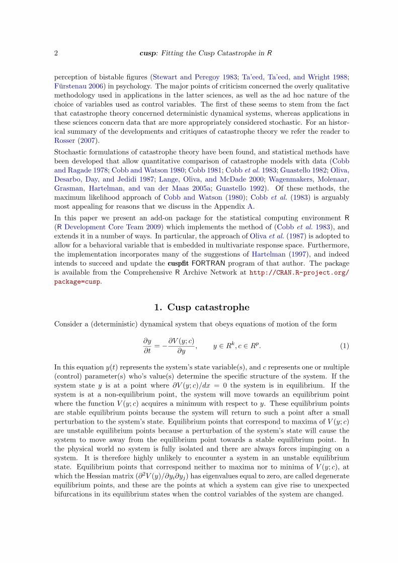
Figure 2: Shape of cusp density in different regions of the control plane. Bimodality of thedensity only occurs in the “bifurcation set”, the cusp shaped shaded area of the control plane.

cusp catastrophe does a better job at describing the data than other conceivable models forthe data.

A difficulty that arises when constructing empirically testable catastrophe models is the factthat catastrophe theory applies to deterministic systems as described by Equation 1. Beinginherently deterministic, catastrophe theory cannot be applied directly to systems that aresubject to random influences which is commonly the case for real physical systems, especiallyin the biological and behavioral sciences.

To bridge the gap between determinism of catastrophe theory and applications in stochasticenvironments, Loren Cobb and his colleagues (Cobb and Ragade 1978; Cobb 1980; Cobb andWatson 1980; Cobb and Zacks 1985) proposed to turn catastrophe theory into a stochasticcatastrophe theory by adding to Equation 1 a (white noise) Wiener process, dW (t), withvariance σ2, and to treat the resulting equation as a stochastic differential equation (SDE):

dY =∂V (Y ;α, β)

∂Ydt+ dW (t).


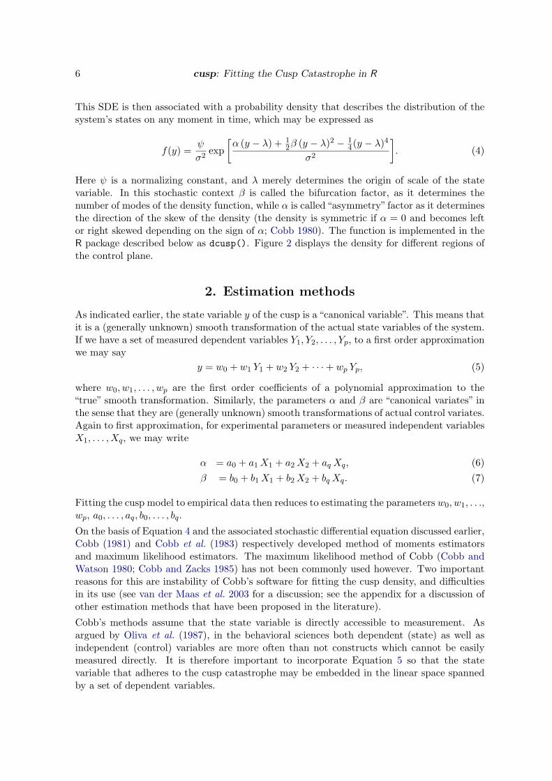
This SDE is then associated with a probability density that describes the distribution of thesystem’s states on any moment in time, which may be expressed as

f(y) =ψ

σ2exp

[α (y − λ) + 1

2β (y − λ)2 − 14(y − λ)4

σ2

]. (4)

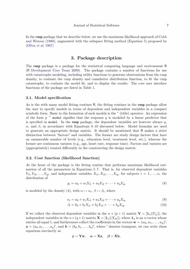
Here ψ is a normalizing constant, and λ merely determines the origin of scale of the statevariable. In this stochastic context β is called the bifurcation factor, as it determines thenumber of modes of the density function, while α is called“asymmetry” factor as it determinesthe direction of the skew of the density (the density is symmetric if α = 0 and becomes leftor right skewed depending on the sign of α; Cobb 1980). The function is implemented in theR package described below as dcusp(). Figure 2 displays the density for different regions ofthe control plane.

2. Estimation methods

As indicated earlier, the state variable y of the cusp is a “canonical variable”. This means thatit is a (generally unknown) smooth transformation of the actual state variables of the system.If we have a set of measured dependent variables Y1, Y2, . . . , Yp, to a first order approximationwe may say

y = w0 + w1 Y1 + w2 Y2 + · · ·+ wp Yp, (5)

where w0, w1, . . . , wp are the first order coefficients of a polynomial approximation to the“true” smooth transformation. Similarly, the parameters α and β are “canonical variates” inthe sense that they are (generally unknown) smooth transformations of actual control variates.Again to first approximation, for experimental parameters or measured independent variablesX1, . . . , Xq, we may write

α = a0 + a1X1 + a2X2 + aqXq, (6)β = b0 + b1X1 + b2X2 + bqXq. (7)

Fitting the cusp model to empirical data then reduces to estimating the parameters w0, w1, . . .,wp, a0, . . . , aq, b0, . . . , bq.

On the basis of Equation 4 and the associated stochastic differential equation discussed earlier,Cobb (1981) and Cobb et al. (1983) respectively developed method of moments estimatorsand maximum likelihood estimators. The maximum likelihood method of Cobb (Cobb andWatson 1980; Cobb and Zacks 1985) has not been commonly used however. Two importantreasons for this are instability of Cobb’s software for fitting the cusp density, and difficultiesin its use (see van der Maas et al. 2003 for a discussion; see the appendix for a discussion ofother estimation methods that have been proposed in the literature).

Cobb’s methods assume that the state variable is directly accessible to measurement. Asargued by Oliva et al. (1987), in the behavioral sciences both dependent (state) as well asindependent (control) variables are more often than not constructs which cannot be easilymeasured directly. It is therefore important to incorporate Equation 5 so that the statevariable that adheres to the cusp catastrophe may be embedded in the linear space spannedby a set of dependent variables.


In the cusp package that we describe below, we use the maximum likelihood approach of Cobband Watson (1980), augmented with the subspace fitting method (Equation 5) proposed by(Oliva et al. 1987)

3. Package description

The cusp package is a package for the statistical computing language and environment R(R Development Core Team 2009). The package contains a number of functions for usewith catastrophe modeling, including utility functions to generate observations from the cuspdensity, to evaluate the cusp density and cumulative distribution function, to fit the cuspcatastrophe, to evaluate the model fit, and to display the results. The core user interfacefunctions of the package are listed in Table 1.

3.1. Model specification

As is the with many model fitting routines R, the fitting routines in the cusp package allowthe user to specify models in terms of dependent and independent variables in a compactsymbolic form. Basic to the formation of such models is the ~ (tilde) operator. An expressionof the form y ~ model signifies that the response y is modeled by a linear predictor thatis specified in model. In the cusp package, the dependent variables are however always y,α, and β, in accordance with Equations 8–10 discussed below. Model formulas are usedto generate an appropriate design matrix. It should be mentioned that R makes a strictdistinction between “factors” and variables. The former are study design factors that havean enumerable number of levels (e.g., education level, treatment level, etc.), whereas theformer are continuous variates (e.g., age, heart rate, response time). Factors and variates are(appropriately) treated differently in the constructing the design matrix.

3.2. Cost function (likelihood function)

At the heart of the package is the fitting routine that performs maximum likelihood esti-mation of all the parameters in Equations 5–7. That is, for observed dependent variablesYi1, Yi2, . . . , Yip, and independent variables Xi1, Xi2, . . . , Xiq, for subjects i = 1, . . . , n, thedistribution of

yi = w0 + w1Yi1 + w2Yi2 + · · ·+ wpYip (8)

is modeled by the density (4), with α 7→ αi, β 7→ βi, where

αi = a0 + a1Xi1 + a2Xi2 + · · ·+ aqXiq (9)βi = b0 + b1Xi1 + b2Xi2 + · · ·+ bqXiq. (10)

If we collect the observed dependent variables in the n × (p + 1) matrix Y = [1n|(Yij)], theindependent variables in the n× (q+1) matrix X = [1n|(Xik)], where 1n is an n-vector whoseentries all equal 1, and furthermore collect the coefficients in the vectors w = (w0, w1, . . . , wp)′,a = (a0, a1, . . . , aq)′, and b = (b0, b1, . . . , bq)′, where ′ denotes transpose, we can write theseequations succinctly as

y = Yw, α = Xa, β = Xb,


Function name Description and example callcusp Fits cusp catastrophe to data.

fit <- cusp(y ~ z, alpha ~ x1 + x2, beta ~ x1 + x2,data)

summary method Computes statistics on parameter estimates and model fit (by de-fault this function compares the cusp model to a linear regressionmodel). For model comparison a pseudo-R2 statistic, AIC and BICare computed.summary(fit)

confint method Computes confidence intervals for the parameter estimates.confint(fit)

vcov method Computes an approximation to the parameter estimator variance-covariance matrix.vcov(fit)

logLik method Returns the optimized value of the log-likelihood.logLik(fit)

plot method Generates a graphical display of the fit, including the estimatedlocations on the cusp control surface for each observation, non-parametric density estimates for different regions of the control sur-face, and a residuals plot. An example is provided in Figure 3. Thegraph is fully customizable.plot(fit)

cusp3d Generates a three dimensional display of the cusp equilibrium sur-face on which the estimated states are displayed. The graphic isfully customizable. Figure 5 displays an example.cusp3d(fit)

cusp3d.surface Generates a three dimensional display of the cusp equilibrium sur-face. Figure 1 was generated with it.cusp3d.surface()

rcusp Generates a random sample from the cusp distribution.y <- rcusp(n = 100, alpha = -1/2, beta = 2)

dcusp, pcuspqcusp The cusp density, cumulative distribution and quantile functions.

dcusp(y = 1.0, alpha = -1/2, beta = 2)cusp.logist Fits an logistic curve to the data. Is used in summary method if op-

tional parameter logist = TRUE is specified for testing the presenceof observations in the bifurcation set.fit <- cusp.logist(y ~ z, alpha ~ x1 + x2, beta ~ x1 +x2, data)

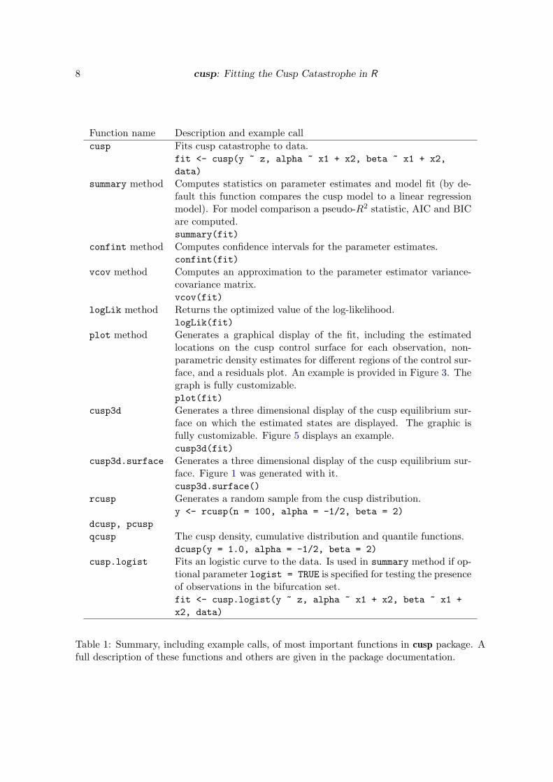
Table 1: Summary, including example calls, of most important functions in cusp package. Afull description of these functions and others are given in the package documentation.


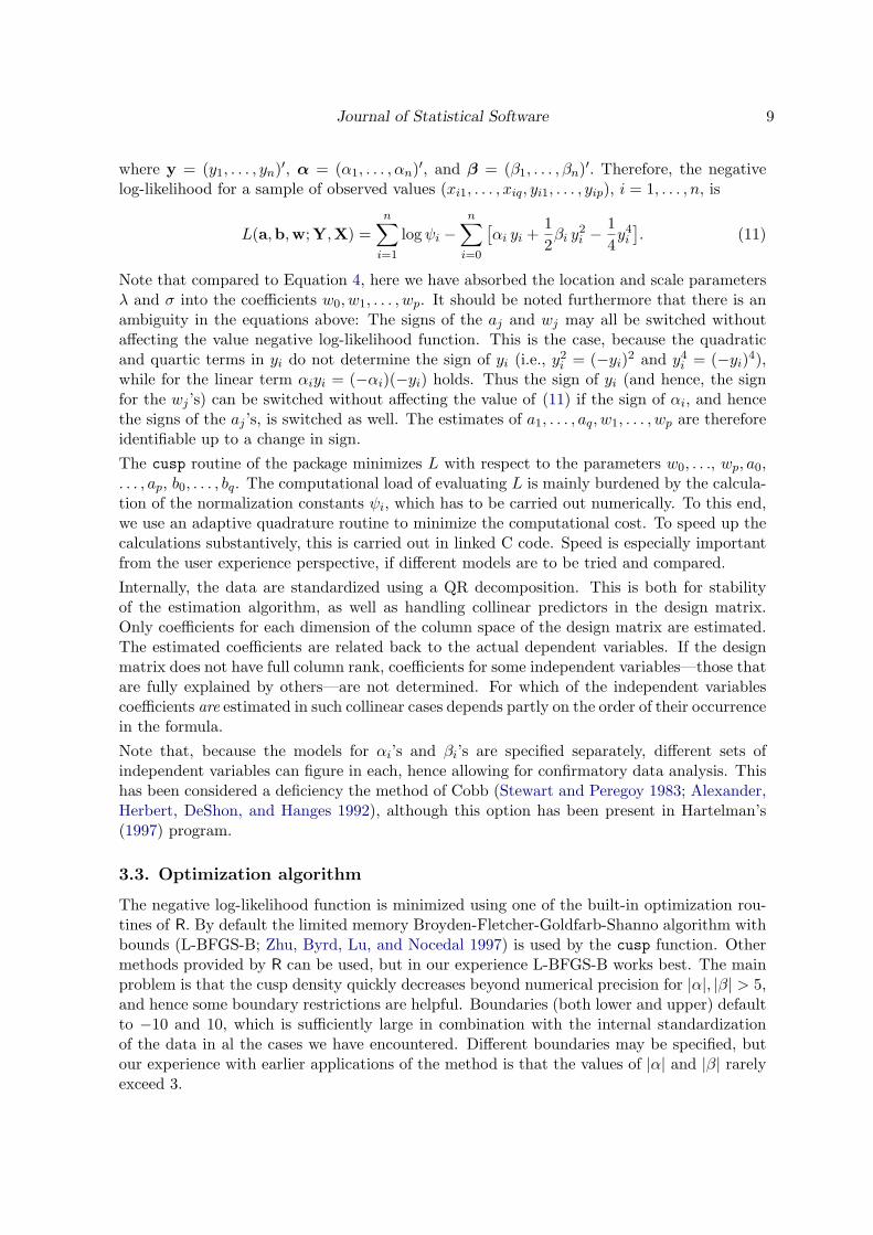
where y = (y1, . . . , yn)′, α = (α1, . . . , αn)′, and β = (β1, . . . , βn)′. Therefore, the negativelog-likelihood for a sample of observed values (xi1, . . . , xiq, yi1, . . . , yip), i = 1, . . . , n, is

L(a,b,w; Y,X) =n∑i=1

logψi −n∑i=0

[αi yi +

12βi y

2i −

14y4i

]. (11)

Note that compared to Equation 4, here we have absorbed the location and scale parametersλ and σ into the coefficients w0, w1, . . . , wp. It should be noted furthermore that there is anambiguity in the equations above: The signs of the aj and wj may all be switched withoutaffecting the value negative log-likelihood function. This is the case, because the quadraticand quartic terms in yi do not determine the sign of yi (i.e., y2

i = (−yi)2 and y4i = (−yi)4),

while for the linear term αiyi = (−αi)(−yi) holds. Thus the sign of yi (and hence, the signfor the wj ’s) can be switched without affecting the value of (11) if the sign of αi, and hencethe signs of the aj ’s, is switched as well. The estimates of a1, . . . , aq, w1, . . . , wp are thereforeidentifiable up to a change in sign.

The cusp routine of the package minimizes L with respect to the parameters w0, . . ., wp, a0,. . . , ap, b0, . . . , bq. The computational load of evaluating L is mainly burdened by the calcula-tion of the normalization constants ψi, which has to be carried out numerically. To this end,we use an adaptive quadrature routine to minimize the computational cost. To speed up thecalculations substantively, this is carried out in linked C code. Speed is especially importantfrom the user experience perspective, if different models are to be tried and compared.

Internally, the data are standardized using a QR decomposition. This is both for stabilityof the estimation algorithm, as well as handling collinear predictors in the design matrix.Only coefficients for each dimension of the column space of the design matrix are estimated.The estimated coefficients are related back to the actual dependent variables. If the designmatrix does not have full column rank, coefficients for some independent variables—those thatare fully explained by others—are not determined. For which of the independent variablescoefficients are estimated in such collinear cases depends partly on the order of their occurrencein the formula.

Note that, because the models for αi’s and βi’s are specified separately, different sets ofindependent variables can figure in each, hence allowing for confirmatory data analysis. Thishas been considered a deficiency the method of Cobb (Stewart and Peregoy 1983; Alexander,Herbert, DeShon, and Hanges 1992), although this option has been present in Hartelman’s(1997) program.

3.3. Optimization algorithm

The negative log-likelihood function is minimized using one of the built-in optimization rou-tines of R. By default the limited memory Broyden-Fletcher-Goldfarb-Shanno algorithm withbounds (L-BFGS-B; Zhu, Byrd, Lu, and Nocedal 1997) is used by the cusp function. Othermethods provided by R can be used, but in our experience L-BFGS-B works best. The mainproblem is that the cusp density quickly decreases beyond numerical precision for |α|, |β| > 5,and hence some boundary restrictions are helpful. Boundaries (both lower and upper) defaultto −10 and 10, which is sufficiently large in combination with the internal standardizationof the data in al the cases we have encountered. Different boundaries may be specified, butour experience with earlier applications of the method is that the values of |α| and |β| rarelyexceed 3.


3.4. Starting point

The starting values used by default turn out to often render convergence of the optimizationalgorithm without problems. When convergence problems arise a warning is issued, and thismay be interpreted as an invitation to the user to provide alternative starting values. In ourexperience convergence to a proper minimum of the negative log-likelihood can be achievedmost of the time by providing alternative starting values. A strong indication of improperconvergence is a warning about NaN’s that is issued when summary statistics are computed.If this happens, the model should be refit using a different set of starting values.

3.5. Statistical evaluation of model fit

To assess the correspondence of data with the predictions made by the cusp catastrophe, anumber of diagnostic tools have been suggested.

Maxwell vs delay convention and R2

First of all, Cobb (1998)—see also Stewart and Peregoy (1983) and Hartelman (1997)—havesuggested a pseudo-R2 as a measure of explained variance defined by

1− error varianceVar(y)

. (12)

This is clearly inspired by the familiar relation between the squared (multiple) correlationcoefficient and the “explained variance” from ordinary regression. However, the term “errorvariance” needs to be defined, which is not trivial for the cusp catastrophe model.

As indicated previously, the cusp catastrophe is not an ordinary regression model. Rather,it is an implicit regression model of an irregular type.1 As such, unlike ordinary regressionmodels, for a given set of values of the independent variables the model may predict multiplevalues for the dependent variable. In ordinary regression the predicted value is usually theexpected value of the dependent variable given the values of the independent variables. Inthe case of the cusp density, for certain values of α and β the cusp density is bimodal, andthe expected value of this density lies in a region of low probability between the two modi.That is, the mathematical expectation of the cusp density is a value that in itself is relativelyunlikely to be observed. Two alternatives for the expected value as the predicted value can beused, which are closely related to a similar problem regarding interpretation conventions indeterministic catastrophe theory: One can choose the mode of the density closest to the statevalues as the predicted value, or one can use the mode at which the density is highest. Theformer is known as the delay convention, the latter as the Maxwell convention. Although inthe physical sciences both have their uses, Cobb and Watson (1980) and Cobb (1998) suggestto use the delay convention (Stewart and Peregoy 1983). Both conventions are provided bythe package, the default being the delay convention.

Hence, in the pseudo-R2 statistic defined above, the error variance is defined as the varianceof the differences between the observed (or estimated) states and the mode of the distributionthat is closest to this value. It should be noted however that this pseudo-R2 can becomenegative if many of the αi’s deviate from 0 in the same direction—in that case the distribution

1The cusp catastrophe is an irregular implicit regression model in the sense that the available statisticaltheory for implicit regression models cannot be applied to catastrophe models (Hartelman 1997).


is strongly skewed, and deviation from the mode is on average larger than deviation from themean. Negative pseudo-R2’s are thus perfectly legitimate for the cusp density, which limitsits value for model fit assessment. Alternatives to the pseudo-R2 are discussed below.

AIC, BIC and logistic curve

In addition to the pseudo-R2 statistic, to establish convincingly the presence of a cusp catas-trophe, Cobb gives three guidelines for evaluating the model fit (Cobb 1998; Hartelman 1997):First, the fit of the cusp should be substantially better than multiple linear regression—i.e., itslikelihood should be significantly higher than that of the ordinary regression model. Second,any of the coefficients w1, . . . , wp should deviate significantly from zero (w0 does not have to),as well as at least one of the aj ’s or bj ’s. Thirdly, at least 10% of the (αi, βi) pairs should liewithin the bifurcation region. The former two guidelines can be assessed with the summaryfunction of the packages; the latter guideline can be assessed with the plot function; both ofthese are detailed in the Examples section below.

A problem arises when the general case of Equation 8 with more than one dependent variableis used: The linear regression model with which to compare the cusp model is not uniquelydefined. The most natural approach seems to be linear subspace regression: The first canonicalvariate between the Xji’s and the Yki’s is used as the predicted value, and the first canonicalcorrelation is used for calculating the explained and residual variance. For models in which(8) contains only one dependent variable this automatically reduces to standard univariatelinear regression.

The 10% guideline of Cobb is somewhat arbitrary, and Hartelman (1997); Hartelman, vander Maas, and Molenaar (1998); van der Maas et al. (2003) propose a more stringent test ofthe presence of bifurcation points: They suggest to compare the model fit to the non-linearleast squares regression to the logistic curve

yi =1

1 + e−αi/β2i

+ εi, i = 1, . . . , n, (13)

where yi, αi, βi are defined in Equations 8–10, and the εi’s are zero mean random disturbances.(One may assume εi to be normally distributed, but this is not necessary; see e.g., Seberand Wild 1989.) The rationale for the logistic function is that this function does not possesdegenerate critical points, while it does have the possibility to model arbitrarily steep changesin the (canonical) state variable as a function of minute changes in an independent variable,thus mimicking “sudden” transitions of the cusp (Hartelman 1997). The summary function inthe package provides an option to fit this logistic curve to the data. Because the cusp densityand the logistic functions are not nested models, the fit cannot be assessed on the basis ofdifferences in the likelihood, and one has to resort to other indicators such as AIC and BIC.These fit indices are both computed by the summary function, as well as an AIC correctedfor small sample sizes (AICc; Burnham and Anderson 2004).

Instead of the 10% guideline, Hartelman (1997) proposes to require that the AIC and BICindicate a better fit for the cusp density than for the logistic curve. Wagenmakers, van derMaas, and Molenaar (2005b) suggest to use the BIC of both models to compute approxima-tion of the posterior odds for the cusp relative to the logistic curve, assuming equal priorprobabilities for both models.


4. Examples

For illustration purposes, we provide three example analyses with the package. The first twoexamples entail data that have been analyzed with cusp catastrophe methods before and havebeen published elsewhere.

Example I

The first example is taken from van der Maas et al. (2003), and concerns attitudinal responsetransitions with respect to the statement “The government must force companies to let theirworkers benefit from the profit as much as the shareholders do”. Some 3000 Dutch respondentsindicated their level of agreement with this statement on a 5 point scale (1 = totally agree,5 = totally disagree). As a normal factor political orientation (measures on a 10 point scalefrom 1 = left wing to 10 = right wing) was used. As a bifurcation factor the total score on a12 item “political involvement” scale was used. The theoretical social psychological details arediscussed in (van der Maas et al. 2003). The data thus consist of a table with three columns:Orient, Involv, and Attitude.

We use the same subset of 1387 cases that was also analyzed in van der Maas et al. (2003). Inthat paper an extensive comparison of models was done. These data are made available in thepackage and can be loaded using the data("attitudes") command. Here we only presentthe analysis for the best fitting model (model 12 in van der Maas et al. 2003, according toAIC and BIC). In that model, the bifurcation factor (βi) is determined exclusively by Involv,while the normal factor (αi) is determined by both Orient and Involv. This model can befitted with the command

R> fit <- cusp(y ~ Attitude, alpha ~ Orient + Involv, beta ~ Involv,

+ data = attitudes, start = attitudeStartingValues)

Here attitudes is the data.frame in which the table with data is stored, and the vectorattitudeStartingValues is a set starting values that is included in the package to obtain asolution quickly for this example. Both were loaded with a data call. Note the use of formula’sdiscussed earlier: The first formula specifies that the state variable yi is determined by thevariable Attitude for which a location and scaling parameter (w0 and w1 in Equation 8)have to be estimated. The second formula states that the normal factor αi is determined bythe variables Orient and Involv for which regression coefficients and an intercept must beestimated. Similarly the third formula which specifies that the bifurcation factor is determinedby the variable Involv for which an intercept and a regression coefficient have to be estimated.When the cusp function returns, the estimates can be printed to the console window of Rby typing print(fit).More informative however is a summary of the parameters and theassociated statistics, which is obtained with the statement

R> summary(fit, logist = TRUE)

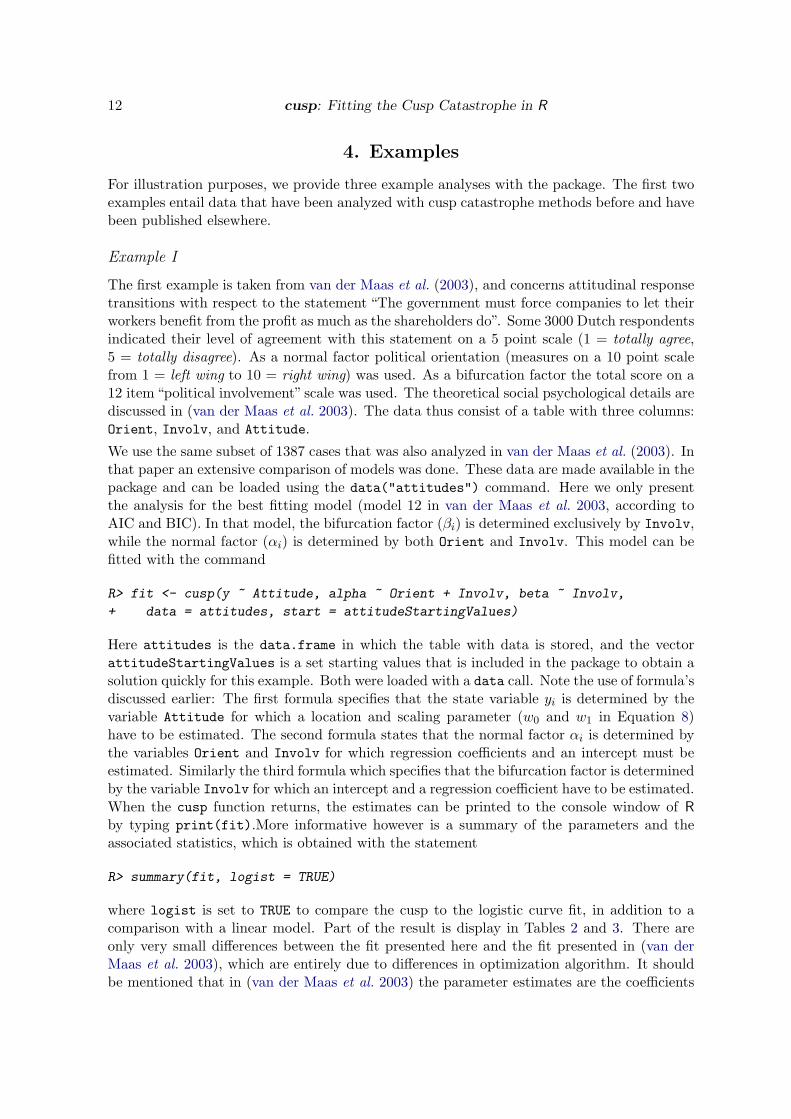
where logist is set to TRUE to compare the cusp to the logistic curve fit, in addition to acomparison with a linear model. Part of the result is display in Tables 2 and 3. There areonly very small differences between the fit presented here and the fit presented in (van derMaas et al. 2003), which are entirely due to differences in optimization algorithm. It shouldbe mentioned that in (van der Maas et al. 2003) the parameter estimates are the coefficients


Estimate Std. Error z value P(> |z|)a[(Intercept)] 0.15271 0.56218 0.272 0.7859a[Orient]∗ 0.46210 0.06414 7.204 < 0.0001a[Involv] 0.09736 0.05445 1.788 0.0738b[(Intercept)] 0.12397 0.38643 0.321 0.7484b[Involv]∗ 0.22738 0.02993 7.597 < 0.0001w[(Intercept)] 0.10543 0.24485 0.431 0.6668w[Attitude]∗ 0.87758 0.06682 13.134 < 0.0001

Table 2: Coefficient summary table for attitudes example obtained with the summary method.

R2 AIC AICc BICLinear model 0.1309 3997.6 3997.6 4018.5Logist model 0.1599 3954.5 3954.5 3985.9Cusp model −0.0962 3623.8 3623.9 3660.4

Table 3: Model fit statistics for synthetic data example as obtained with summary. Thecolumn labeled “R2” gives conventional R2 for the linear and logist model, and the pseudo-R2

statistic for the cusp model.

with respect to standardized data. To standardize the data the scale function of R can beused. The column headed “R2” in Table 3 lists the squared multiple correlation for the linearregression model and logistic curve model, and the pseudo-R2 for the cusp catastrophe model.

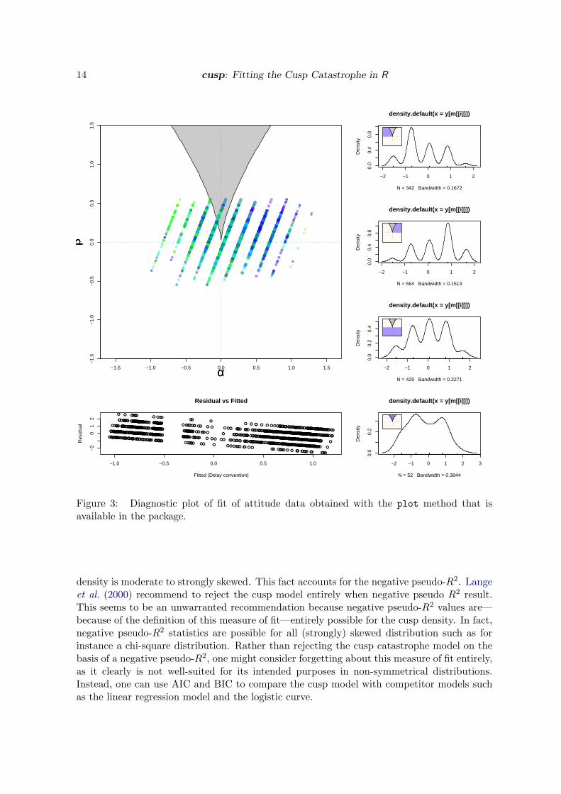
A visual display of the data fit and diagnostic plots is generated with the command plot(fit);the result is displayed in Figure 3. The figure display the control plane along with theestimated (αi, βi), i = 1, . . . , n, for each of the observations. Furthermore, it (optionally)displays for each of four regions in the control plane a density estimate of the estimatedstate variable in that region. These are displayed on the right in the figure: The top twopanels reflect the densities in the region left and right of the bifurcation region respectively.These should be positively skewed for the left side and negatively skewed for the right side(compare Figure 2). The next panel display the density estimate for the state estimatesbelow the bifurcation region. Here the density estimate should be approximately uni-modaland less skewed than in the other two regions. The last panel displays the density estimatefor estimated state values within the bifurcation region. In this region the density should bebimodal. For the data displayed here the first three densities seem heavily multi-modal. Thisis due to the fact that the bifurcation factor “political orientation” was measured on a discreteordinal 10 points scale, thus artifactually introducing modes around these values. The residualversus fitted plot displays the estimated errors as a function of predicted states. As indicatedearlier, by default the errors are computed using the delay convention. Although with a goodmodel fit one would expect to see no systematic relationship between the estimated errorsand the predicted states, we have observed a consistent negative trend between the two—evenwhen the data were generated from the cusp density in simulations. This may simply resultfrom cases of which the density is strongly skewed. Hence, a slight negative trend should notbe taken too seriously as an indication of model misfit.

Note from Figure 3 that the overwhelming majority of cases lie in regions where the cusp


−1.5 −1.0 −0.5 0.0 0.5 1.0 1.5

−1.

5−

1.0

−0.

50.

00.

51.

01.

5

αα

ββ

●

●

●

●

●

● ● ●

●●

●

●

●● ●

●

●

●

●

●

●

●

●

●

●

●●

●●

●

●

●

●

●

●

●

●

●●

●

●

●

●

●

● ●

● ●

●●

● ●●

●

●

●

●

●

●

●●

●

●●

●

●●

●

●

●

●●

●●

●●

●●●

●●

● ●

●

●

●

●

●

●

●

●●

●

●

●

●

●

●

●●

●

●

●

●●

●

●

●

●●

●● ●●●

●

●

●

●

●

●

●

●

●●● ● ●

●

●

●●

●

●

●

●

●●

●

●

●

●

●

●●

●

●

●●●

●

● ●●

●

●

●●

●●● ●

● ●

●

●

●

●●

●

●

●

●●●

●

●

●●●

●

●

●

● ●

● ●

●

●

●●

●

●●

●●

●

●●

●

●

●

●

●

●

● ●●

●

●

●

●

●

●

●

●● ●

●● ●

●

●

●

●●

●

●●

●

●

● ●

●

●

●

●

●

●●

●●

●●

●

●●

●

● ●

●

●

●

●

●●

●●

●

●

●●

●●

●

●●

●

●

●

●

●

●

●●

●●●

●●

●●

●

●●

● ●

●

●

●

●

●●

●

●● ●●

●

●

●

●

●

●

●

●●

●

●●

●

●

● ●●

●● ●●

●●●

●●

●

●

●

●

●

●

●

●●

●

● ●

●● ● ●

●

●

●

●

●

●●

●●

●

●

●

●

●

●

●

●

●● ●●

●●

●●

●

● ●

●

●●

●

●

●

●

●

●

●

●

●

● ●●

●●

●

●

●●

●

●

●●●●

●

●

●●

●●

●

● ●

●

●

●

●●

●●

●

●●

●

●

●

●

● ●

●

● ●●

●

● ●●

●● ●

●

●

●

●

●

●

●

●●

● ●●

●

●

●

●

●

● ●

●

●

● ●

●

● ●●

●

●●

●

●

●

●

●●

●

●

●●

●●

●

●●

●●

●●

●

●●

●

●

●

●●●

●

●

● ●

●

●●

●

●

●

●

●● ●

●

●

●●

●

●

● ●

●

●

●

●●

●

●

●● ●

●

●

●

●

●

●●

●

●

●

●

●

●

● ●

●

●●●

●

●

●●

●●

●

●

●

●

●

●

●

●

●

●●●

●

●

●

●●

●

●

●●●

●

●

●●

●●

●

●

●

●●

●●

●

●

●

●

●

●

●●●●

●

●●

●

●●

●

●

●

●

●

●

●

●

●

●

●

●●●

●

●

●

● ●

●●

●●●

●

●

●

●

●●

●●

● ●

●●

●● ●

●

●● ●●

●●

●

●●

●

●

●●●●

●

●

●

●

● ●

●

●

●●●

●

●●

●

●

●

●

●

●

●

●

●● ●

●

●

●●

●

●●

●●●

●●

● ●

●

●

●

●●

●

●

●

●●

●

●

●

●

●

●

●●

●●

●●

●

●●●●

●

●

●

●

●

●●

● ●

●●

●

●

●●

●

●

●

●

●

●

●●

●●●

●

●

●

●

●

●

●●

●

●

●

●●

●

●

●

●

●

●

●

●

● ●

●

●

●

●

●

●

● ● ●●

●

●●

●

●●

●

●●

●●

●

●

●

●

●

●●●●

●

●●

●

● ●

●●

●

● ●●

●

●

●●

●

●

●

●

●

●● ●

●

●

●

●

●

●

●● ●

●●

●

●●

●

●

●

●

●

● ●

●

●

●

●

● ●●

●

●

●●

●

●●●

●

●

●

●

●

●

●

●

●●

●

●

●

●

●

●

●

●

●

●

●●

●

●●

●●

●

●

●

●

●

●

●

●

●

●●

●

●●

●●

●

●

●●

●

●

●

●

●

●

●

●

● ●

●

●

● ●●

●

●

●●

●

●

●

●

●

● ●

●

●●●

●

●

●

●●●

●

●

●

●

●

●

●●

● ●

●

●

●

● ●

●

●

●

●

●

●

●●●

●●

●

●

●

●

●

●

●

●

●

●

●●

●

●

●

●●

●●

●

●

●

●

●●●

●

●

●

●

●●

●

●

●

●

●

●

●

●●

●●

●

●●

●

●

●

●

●

●●

●●

●

●

●

● ● ●

●

●

●

●●

●

●●

●●●

●

●

●

●

●

●

●

●

●

●●●●

●

● ●●

●

●●

●

● ● ●●

●●●

●

●● ●●

●

● ●●

●

●●

●

●

●

●

●●●

●

●

●●

●

●●

●

●

●

●

●

●● ●

●

●

●

●

●

●

●

●

● ●

●

●

●

●

●

● ●●

●

●●

●

●

●

●

● ●

●

●

●

●

●

●

●●

●

●●●●

●

●

●

●

●

●

●

●

●

●

●●

●

●

●

●

●

●

●

●

●

●

●

●

●

●●

●

●●

●

●

●

●

●

●

●● ●

●

●

●

●●

●

●

●

● ●

●●●●

●●●

●●

●

●

●

●

●

●

●

●●

●

●

●

●

●

●

●

●

●

●●● ●

●●

●

●

●●

●

●

●

●

●

●

●●

●

●

●

●●

● ●

●

●

●●

●

●

●

●● ●

●

●●

●

●

● ●

● ●

●

●●

●

●

●

● ●●●

●●

●

●

●

●

●●

●

●●

●●● ●

●

●

●

●

●

●

●●

●

●

●

●

●

●

●

●

●

●●

●

●

●

●

●

●

●●

●●

●

●

●

●●●

●

● ●

●

●

●●

●

●●

●

●

●

●

●●

●

●●●●

●

●

●

●

● ●

●●

●

●

●

●

●● ● ●●

●●

●●

●

●●●

●

●

●●

●●

●

●

●

●

●

●

●

●

●

●

● ●

●

●

●

−1.0 −0.5 0.0 0.5 1.0

−2

01

2

Residual vs Fitted

Fitted (Delay convention)

Res

idua

l

−2 −1 0 1 2

0.0

0.4

0.8

density.default(x = y[m[[i]]])

N = 342 Bandwidth = 0.1672

Den

sity

−2 −1 0 1 2

0.0

0.4

0.8


N = 564 Bandwidth = 0.1513

Den

sity

−2 −1 0 1 20.

00.

20.

4


N = 429 Bandwidth = 0.2271

Den

sity

−2 −1 0 1 2 3

0.0

0.2


N = 52 Bandwidth = 0.3844

Den

sity

Figure 3: Diagnostic plot of fit of attitude data obtained with the plot method that isavailable in the package.

density is moderate to strongly skewed. This fact accounts for the negative pseudo-R2. Langeet al. (2000) recommend to reject the cusp model entirely when negative pseudo R2 result.This seems to be an unwarranted recommendation because negative pseudo-R2 values are—because of the definition of this measure of fit—entirely possible for the cusp density. In fact,negative pseudo-R2 statistics are possible for all (strongly) skewed distribution such as forinstance a chi-square distribution. Rather than rejecting the cusp catastrophe model on thebasis of a negative pseudo-R2, one might consider forgetting about this measure of fit entirely,as it clearly is not well-suited for its intended purposes in non-symmetrical distributions.Instead, one can use AIC and BIC to compare the cusp model with competitor models suchas the linear regression model and the logistic curve.


Example II

In the second example we use the model specified by Oliva et al. (1987) to demonstrate the useof multiple state variables. The model corresponds to the data in Table 2 of that paper, whichdisplays synthetic data for 50 cases with scores on two (dependent) state variables (Z1 and Z2),four (independent) bifurcation variables (Y1, Y4, Y4, and Y4), and three (independent) normalvariables (X1, X2, and X3). The data can be loaded from the package with data(oliva).The “true” model for their synthetic data is

αi = X1 − 0.969X2 − 0.201X3,

βi = 0.44Y1 + 0.08Y2 + 0.67Y3 + 0.19Y4, (14)yi = −0.52Z1 − 1.60Z2.

For testing purposes, Oliva et al. (1987) did not add noise to any of the variables, and hence,the data perfectly comply with their implicit regression Equation 3.

Because we are using the stochastic approach of Cobb, we cannot use these deterministic data.We therefore generated data in accordance with the model in Equation 14, where X1, X2,and X3 were uniformly distributed on the interval (−2, 2), Y1, Y2 and Z1 were uniformlydistributed on (−3, 3), and Y3 and Y4 were uniformly distributed on (−5, 5). The statesyi were then generated from the cusp density with their respective α and β as normal andsplitting factors, and then Z2 was computed as Z2i = (yi + 0.52Z1i)/(−1.60).

The call for fitting the model of Oliva et al. (1987) for the resulting data set is

R> oliva.fit <- cusp(y ~ z1 + z2 - 1, alpha ~ x1 + x2 + x3 - 1,

+ beta ~ y1 + y2 + y3 + y4 - 1, data = oliva)

Note that in the model there are no intercept coefficients; this is signified in the cusp call bythe -1 added to the formula’s (see the formula section of the R manual, R Development CoreTeam 2009 for details). The data are stored in the data frame oliva in this case. The resultfrom summary(oliva.fit, logist = TRUE) is displayed in the upper part of Table 4.

Some of the estimates differ substantially from the true values. This should however not betoo surprising given that there are 9 estimated parameters and only 50 observations, yield-ing a ratio of 55/9 ≈ 5.5 observations per parameter. Six coefficients differ significantlyfrom zero: ax1, ax2, by1, by3, and both wz1 and wz2. Using confint to calculate confidenceintervals, we obtain for ax1, ax2, by1, by3, wz1 and wz2 95% confidence intervals of respec-tively (−1.26,−0.3979), (0.2864, 1.0676), (0.1749, 0.7197), (0.5658, 1.07), (0.4074, 0.589) and(1.333, 1.669), which all neatly cover the true values. The same confidence interval for by4however, is (−0.4271, 0.134), which does not contain the true value. This may indicate thatthe estimator is biased. Indeed Hartelman (1997) showed in simulations that the estimatorsare in fact biased. The control factors (αi’s and βi’s) were however recovered quite decently:Correlations between the actual αi’s and those predicted by the model fit (which can be ob-tained with the function predict) was .996, and the correlation between actual βi’s and thosepredicted by the model fit was .924.

In contrast to the model specified in this fit, which is rather informed on the variables andtheir role in the cusp catastrophe, it is often the case that one doesn’t know which variablesdetermine the splitting factor, and which variables determine the normal factor. We thereforealso fitted a less informed model, in which both alpha and beta are specified as x1 + x2


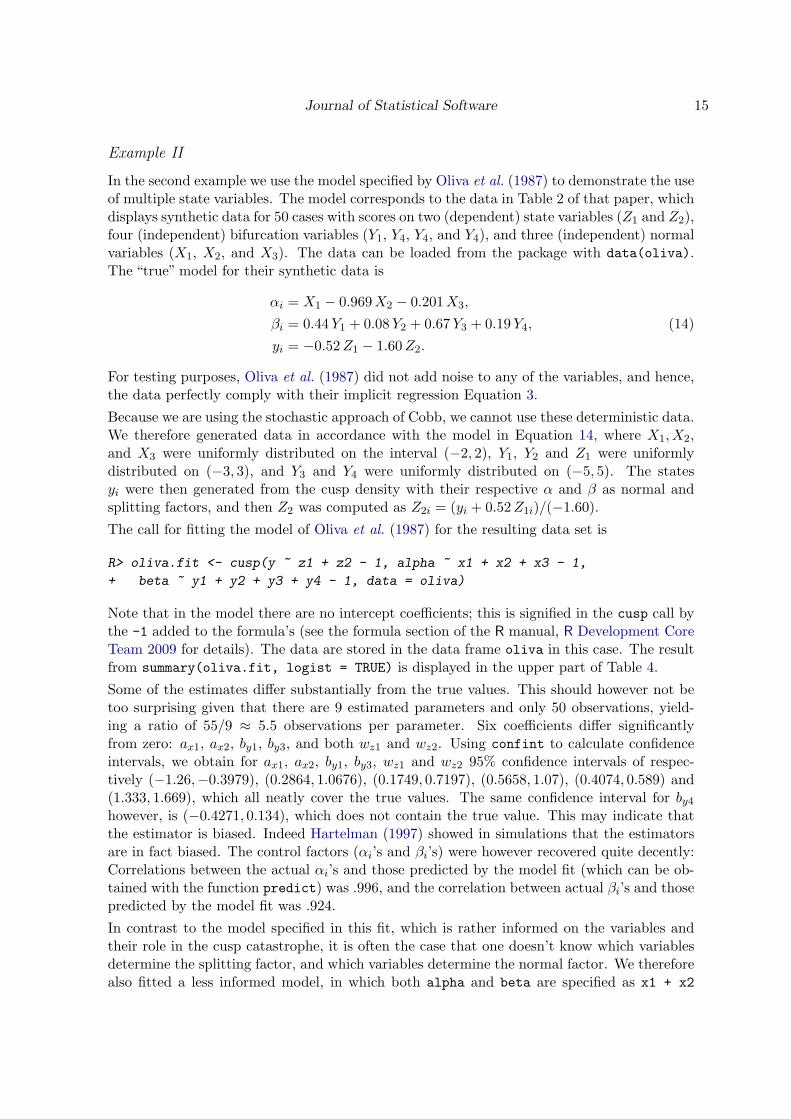
Model IEstimate Std. Error z value P(> |z|)

a[x1]∗ 0.82896 0.21994 3.769 0.0002a[x2]∗ −0.67698 0.19928 −3.397 0.0007a[x3] −0.17317 0.15706 −1.103 0.2702b[y1]∗ 0.44729 0.13899 3.218 0.0013b[y2] 0.24059 0.16021 1.502 0.1332b[y3]∗ 0.81809 0.12873 6.355 < 0.001b[y4] −0.14654 0.14315 −1.024 0.3060w[z1]∗ −0.49822 0.04633 −10.753 < 0.001w[z2]∗ −1.50097 0.08555 −17.545 < 0.001

Model IIEstimate Std. Error z value P(> |z|)

a[(Intercept)] −0.8868 0.6240 −1.4213 0.1552a[x1]∗ −0.9109 0.2564 −3.5527 0.0004a[x2]∗ 0.7251 0.2191 3.3100 0.0009a[x3] 0.1584 0.1735 0.9130 0.3613a[y1] 0.0653 0.0933 0.6998 0.4841a[y2] −0.0341 0.1099 −0.3108 0.7560a[y3] 0.1474 0.1318 1.1182 0.2635a[y4] 0.0590 0.1149 0.5131 0.6079b[(Intercept)] 0.1572 0.9575 0.1642 0.8696b[x1] 0.0317 0.3053 0.1039 0.9173b[x2] −0.3197 0.2690 −1.1883 0.2347b[x3] −0.2083 0.2428 −0.8581 0.3909b[y1]∗ 0.4379 0.1389 3.1528 0.0016b[y2] 0.2794 0.1721 1.6235 0.1045b[y3]∗ 0.7788 0.1983 3.9266 0.0001b[y4] −0.1432 0.1701 −0.8419 0.3999w[(Intercept)] −0.0976 0.1046 −0.9328 0.3509w[z1]∗ 0.4963 0.0493 10.0720 < 0.000w[z2]∗ 1.5186 0.0897 16.9330 < 0.000

Table 4: Coefficient summary table for synthetic data example obtained with summary. Sig-nificant parameters are indicated with an asteriks (∗). Model I: y ~ z1 + z2 - 1, alpha ~ x1+ x2 + x3 - 1, beta ~ y1 + y2 + y3 + y4 - 1. Model II: y ~ z1 + z2, alpha, beta ~ x1+ x2 + x3 + y1 + y2 + y3 + y4.

+ x3 + y1 + y2 + y3 + y4. That is, all independent variables are used to model both thesplitting as well as the normal factor. The resulting estimates are given in the second part ofTable 4. The same set of estimates differs significantly from zero, demonstrating the usefulnessof having significance tests for each estimate separately. The confidence intervals all coveredthe true parameter value, except for the same parameter as in the informed model.

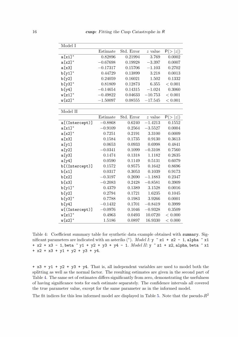
The fit indices for this less informed model are displayed in Table 5. Note that the pseudo-R2


R2 AIC AICc BICLinear model 0.5381 131.72 137.37 150.84Logist model 0.8485 92.17 114.23 126.58Cusp model 0.7821 80.60 105.93 116.93

Table 5: Model fit statistics for Oliva et al. (1987) synthetic data example obtained withsummary for the less informed model (Model II; see text for details). Note: “R2” value forcusp is pseudo-R2.

−4 −2 0 2 4

−4

−2

02

4

αα

ββ

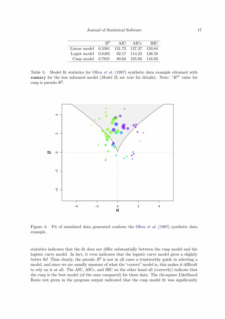
Figure 4: Fit of simulated data generated conform the Oliva et al. (1987) synthetic dataexample.

statistics indicates that the fit does not differ substantially between the cusp model and thelogistic curve model. In fact, it even indicates that the logistic curve model gives a slightlybetter fit! Thus clearly, the pseudo R2 is not in all cases a trustworthy guide in selecting amodel, and since we are usually unaware of what the “correct” model is, this makes it difficultto rely on it at all. The AIC, AICc, and BIC on the other hand all (correctly) indicate thatthe cusp is the best model (of the ones compared) for these data. The chi-square LikelihoodRatio test given in the program output indicated that the cusp model fit was significantly


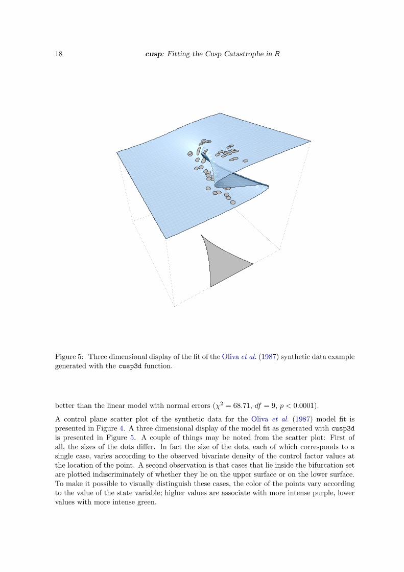
Figure 5: Three dimensional display of the fit of the Oliva et al. (1987) synthetic data examplegenerated with the cusp3d function.

better than the linear model with normal errors (χ2 = 68.71, df = 9, p < 0.0001).

A control plane scatter plot of the synthetic data for the Oliva et al. (1987) model fit ispresented in Figure 4. A three dimensional display of the model fit as generated with cusp3dis presented in Figure 5. A couple of things may be noted from the scatter plot: First ofall, the sizes of the dots differ. In fact the size of the dots, each of which corresponds to asingle case, varies according to the observed bivariate density of the control factor values atthe location of the point. A second observation is that cases that lie inside the bifurcation setare plotted indiscriminately of whether they lie on the upper surface or on the lower surface.To make it possible to visually distinguish these cases, the color of the points vary accordingto the value of the state variable; higher values are associate with more intense purple, lowervalues with more intense green.


control planey

x

● fixed point

central axis

●

●

● strap pointz

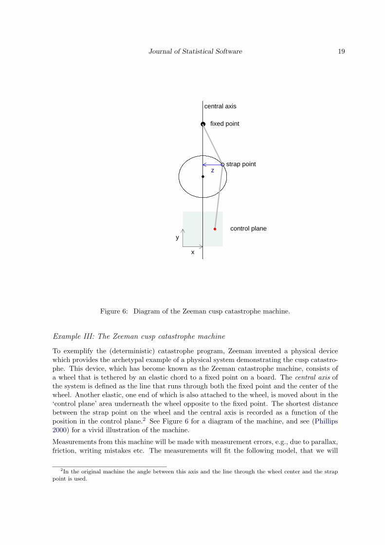
Figure 6: Diagram of the Zeeman cusp catastrophe machine.

Example III: The Zeeman cusp catastrophe machine

To exemplify the (deterministic) catastrophe program, Zeeman invented a physical devicewhich provides the archetypal example of a physical system demonstrating the cusp catastro-phe. This device, which has become known as the Zeeman catastrophe machine, consists ofa wheel that is tethered by an elastic chord to a fixed point on a board. The central axis ofthe system is defined as the line that runs through both the fixed point and the center of thewheel. Another elastic, one end of which is also attached to the wheel, is moved about in the‘control plane’ area underneath the wheel opposite to the fixed point. The shortest distancebetween the strap point on the wheel and the central axis is recorded as a function of theposition in the control plane.2 See Figure 6 for a diagram of the machine, and see (Phillips2000) for a vivid illustration of the machine.

Measurements from this machine will be made with measurement errors, e.g., due to parallax,friction, writing mistakes etc. The measurements will fit the following model, that we will

2In the original machine the angle between this axis and the line through the wheel center and the strappoint is used.


Estimate Std. Error z value P(> |z|)a[(Intercept)] 0.21470 0.25516 0.841 0.40011a[x]∗ 1.15341 0.15558 7.414 1.23e-13a[y] −0.16460 0.11996 −1.372 0.17002b[(Intercept)]∗ 1.04763 0.37401 2.801 0.00509b[x] 0.02851 0.14058 0.203 0.83927b[y]∗ −1.48202 0.13634 −10.870 < 2e-16w[(Intercept)] −0.02387 0.13178 −0.181 0.85625w[z]∗ 0.90316 0.02723 33.168 < 2e-16

Table 6: Coefficient summary table for zeeman1 data set obtained with summary. The modelspecification was y ~ z, alpha ~ x + y, beta ~ x + y.

R2 AIC AICc BICLinear model 0.8711298 348.8954 349.1713 360.9379Logist model 0.9749158 109.4103 110.1990 130.4847Cusp model 0.9554786 −136.4639 −135.4426 −112.3788

Table 7: Model fit statistics for zeeman1 data obtained with summary. Note: The R2 valuefor cusp is pseudo-R2.

dub the measurement error model:

yi = zi + εi, i = 1, . . . , n,

where εi is a zero mean random variable, e.g., εi ∼ N(0, σ2) for some σ2, and zi is one of theextremal real roots of the cusp catastrophe equation

αi + βiz − z3 = 0.

Note that this model is quite different from Cobb’s conceptualization of the stochastic cuspcatastrophe. The cusp package is intended for the latter model (i.e., for Cobb’s stochasticcatastrophe model), however, the data from the Zeeman catastrophe machine below showthat it is also quite accomodating for the measurement error model.The data, that were recorded using a physical instance of the machine and a measurementtape, are available in the package as zeeman1.3 The data set contains 150 observations fromthe state variable z (the shortest distance of the strap point on the wheel to the central axis)as a function of the bifurcation variable labeled y (running parallel to the central axis), andthe asymmetry variable labeled x (running orthogonal to the central axis). The control planewas sampled on a regular grid.A fit of the cusp density to these data, which actually conform to the measurement errormodel and not to the cusp SDE of Cobb, using the command

R> fit.zeeman <- cusp(y ~ z, alpha ~ x + y, beta ~ x + y, data = zeeman1)

R> summary(fit.zeeman)

3In fact three data sets from three different instances recorded by separate individuals are available aszeeman1, zeeman2, and zeeman3.


Zeeman Cusp Catastrophe Machine Data

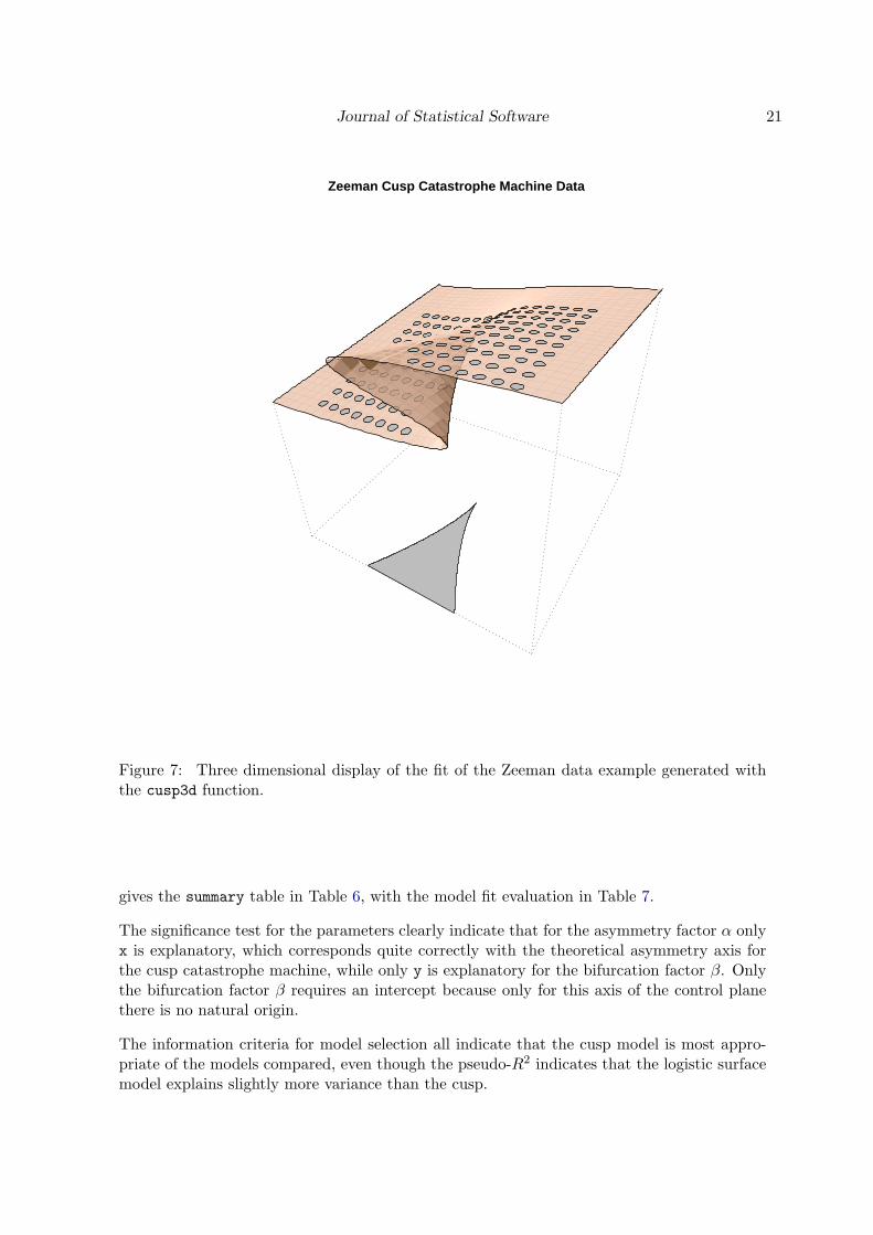
Figure 7: Three dimensional display of the fit of the Zeeman data example generated withthe cusp3d function.

gives the summary table in Table 6, with the model fit evaluation in Table 7.

The significance test for the parameters clearly indicate that for the asymmetry factor α onlyx is explanatory, which corresponds quite correctly with the theoretical asymmetry axis forthe cusp catastrophe machine, while only y is explanatory for the bifurcation factor β. Onlythe bifurcation factor β requires an intercept because only for this axis of the control planethere is no natural origin.

The information criteria for model selection all indicate that the cusp model is most appro-priate of the models compared, even though the pseudo-R2 indicates that the logistic surfacemodel explains slightly more variance than the cusp.


5. Discussion

In this paper we have presented an add-on package for cusp catastrophe modeling in R. Thecore user interface functions allow the user to easily specify and fit a broad range of modelsusing the maximum likelihood approach of Cobb (Cobb 1980; Cobb and Watson 1980). Italso provides the user a number of tools for the assessment of the cusp catastrophe model fit.

Although the focus of this paper was entirely on quantitative methodology, by no means dowe consider the statistically satisfactory fit of a cusp catastrophe model—or any catastrophymodel for that matter—definite evidence for the for the presence of dynamical phase transi-tions. Without concurrent qualitative assessment of the presence of catastrophe flags impliedby the model, and without a sound theoretical framework that implicates an underlying gra-dient system near equilibrium states, any catatrophe model fit remains unconvincing.

Cobb’s method is not without it limitations. Deterministic catastrophe classifies systems upto a set of smooth nonlinear scalings of the state variables. Hartelman (1997) points out thatthis poses a problem for Cobb’s approach. The alternative approach offered in (Hartelman1997; see also Wagenmakers et al. 2005a) however, only works for time series. Practicalexperience with applications to cross-sectional data indicates that Cobb’s method is suitablefor these cases.

A number of improvement of the package can be thought of. The current package tests forthe presence of bifurcation points by fitting a logistic curve that accommodates arbitrarilysudden changes in the state variable as a function of smooth gradual changes in the controlvariables. More ideally, to test for the presence of bifurcation points one should minimize thenegative log-likelihood L of Equation 11 subject to the n constraints δi = α2

i /4− β3i /27 ≤ 0.

The parameter δi is known as Cardan’s Discriminant, named after the 16th century Italianmathematician who first published it (Cobb and Zacks 1985). It is positive, only if the cuspEquation 3 has three solutions–i.e., only if there are multiple equilibrium states. One then canuse likelihood ratio chi-square testing to compare this model with the unconstrained model.This could be a viable alternative approach to the logistic curve fit, but it would require adifferent optimization routine. Unfortunately, R currently has no optimization routine thatallows for arbitrary nonlinear inequality constraints.

One might further consider a Bayesian approach to estimation. The Bayesian approach how-ever, comes of course at the cost of having to specify a prior belief about the likelihood ofparameter values. Given the relations between parameters w0, w1, . . . , bq−1, bq and the data inEquations 8–10 the latter seems rather laborious in the most general case, and a far from in-tuitive enterprise. Only (relatively) uninformative priors seem straightforward, hence leavingout the heart of a true Bayesian approach.

These considerations will be explored in future improvements of the package.

Acknowledgments

Preparation of this article was sponsored in part by a VENI-grant and a COF-grant from theNetherland Organisation for Scienctific research (NWO).


References

Alexander RA, Herbert GR, DeShon RP, Hanges PJ (1992). “An Examination of Least–Squares Regression Modeling of Catastrophe-Theory.” Psychological Bulletin, 111(2), 366–374.

Burnham K, Anderson D (2004). “Multimodel Inference: Understanding AIC and BIC inModel Selection.” Sociological Methods & Research, 33, 261–304.

Cobb L (1980). “Estimation Theory for the Cusp Catastrophe Model.” Proceedings of theSection on Survey Research Methods, pp. 772–776.

Cobb L (1981). “Parameter Estimation for the Cusp Catastrophe Model.” Behavioral Science,26(1), 75–78.

Cobb L (1998). “An Introduction to Cusp Surface Analysis.” Technical report, Aetheling Con-sultants, Louisville, CO, USA. URL http://www.aetheling.com/models/cusp/Intro.htm.

Cobb L, Koppstein P, Chen N (1983). “Estimation and Moment Recursion Relations forMultimodal Distributions of the Exponential Family.” Journal of the American StatisticalAssociation, 78(381), 124–130.

Cobb L, Ragade RK (1978). “Applications of Catastrophe Theory in the Behavioral and LifeSciences.” Behavioral Science, 23, 291–419.

Cobb L, Watson B (1980). “Statistical Catastrophe Theory: An Overview.” MathematicalModelling, 1(4), 311–317.

Cobb L, Zacks S (1985). “Applications of Catastrophe Theory for Statistical Modeling in theBiosciences.” Journal of the American Statistical Association, 80(392), 793–802.

Furstenau N (2006). “Modelling and Simulation of Spontaneous Perception Switching withAmbiguous Visual Stimuli in Augmented Vision Systems.” Perception and Interactive Tech-nologies, 4021, 20–31.

Gilmore R (1993). Catastrophe Theory for Scientists and Engineers. Dover, New York, NY,USA.

Guastello SJ (1982). “Moderator Regression and the Cusp Catastrophe – Application of 2–Stage Personnel-Selection, Training, Therapy, and Policy Evaluation.” Behavioral Science,27(3), 259–272.

Guastello SJ (1988). “Catastrophe Modeling of the Accident Process: Organizational SubunitSize.” Psychological Bulletin, 103(2), 246–255.

Guastello SJ (1992). “Clash of the Paradigms – A Critique of an Examination of the Polyno-mial Regression Technique for Evaluating Catastrophe-Theory Hypotheses.” PsychologicalBulletin, 111(2), 375–379.

Hartelman PAI (1997). Stochastic Catastrophe Theory. Ph.D. thesis, University of Amster-dam, Amsterdam, the Netherlands.

http://www.aetheling.com/models/cusp/Intro.htm

http://www.aetheling.com/models/cusp/Intro.htm


Hartelman PAI, van der Maas HLJ, Molenaar PCM (1998). “Detecting and Modelling Devel-opmental Transitions.” British Journal of Developmental Psychology, 16, 97–122.

Isnard C, Zeeman E (1976). “Some Models from Catastrophe Theory in the Social Sciences.”In L Collins (ed.), The Use of Models in the Social Sciences. Tavistock, London, UK.

Lange R, Oliva TA, McDade S (2000). “An Algorithm for Estimating Multivariate Cas-tastrophe Models: GEMCAT II.” Studies in Nonlinear Dynamics & Econometrics, 4(3),169–182.

Oliva T, Desarbo W, Day D, Jedidi K (1987). “GEMCAT: A General Multivariate Method-ology for Estimating Catastrophe Models.” Behavioral Science, 32(2), 121–137.

Phillips T (2000). “Doctor Zeeman’s Original Catastrophe Machine.” Webpage. URL http://www.math.sunysb.edu/~tony/whatsnew/column/catastrophe-0600/cusp4.html.

Poston T, Stewart I (1996). Catastrophe Theory and Its Applications. Dover, New York.

R Development Core Team (2009). R: A Language and Environment for Statistical Computing.R Foundation for Statistical Computing, Vienna, Austria. ISBN 3-900051-07-0, URL http://www.R-project.org/.

Rosser J (2007). “The Rise and Fall of Catastrophe Theory Applications in Economics: Wasthe Baby Thrown Out with the Bathwater?” Journal of Economic Dynamics and Control,31(10), 3255–3280.

Seber GAF, Wild CJ (1989). Nonlinear Regression. John Wiley & Sons, New York, NY,USA.

Stewart IN, Peregoy PL (1983). “Catastrophe-Theory Modeling in Psychology.” PsychologicalBulletin, 94(2), 336–362.

Sussmann HJ, Zahler RS (1978). “Catastrophe Theory as Applied To the Social and BiologicalSciences: A Critique.” Synthese, 37(2), 117–216.

Ta’eed LK, Ta’eed O, Wright JE (1988). “Determinants Involved in the Perception of theNecker Cube: An Application of Catastrophe Theory.” Behavioral Science, 33(2), 97–115.

Thom R (1973). Structural Stability and Morphogenesis: Essai D’une Theorie Generale DesModeles. W. A. Benjamin, California.

Thom R, Fowler DH (1975). Structural Stability and Morphogenesis: An Outline of a GeneralTheory of Models. W. A. Benjamin, Michigan.

van der Maas HLJ, Kolstein R, van der Pligt J (2003). “Sudden Transitions in Attitudes.”Sociological Methods & Research, 23(2), 125–152.

van der Maas HLJ, Molenaar PCM (1992). “Stagewise Cognitive Development: An Applica-tion of Catastrophe Theory.” Psychological Review, 99(3), 395–417.

Wagenmakers EJ, Molenaar PCM, Grasman RPPP, Hartelman PAI, van der Maas HLJ(2005a). “Transformation Invariant Stochastic Catastrophe Theory.” Physica D, 211, 263–276.

http://www.math.sunysb.edu/~tony/whatsnew/column/catastrophe-0600/cusp4.html

http://www.math.sunysb.edu/~tony/whatsnew/column/catastrophe-0600/cusp4.html

http://www.R-project.org/

http://www.R-project.org/


Wagenmakers EJ, van der Maas HLJ, Molenaar PCM (2005b). “Fitting the Cusp CatastropheModel.” In BS Everitt, DC Howell (eds.), Encyclopedia of Statistics in Behavioral Science,volume 1, pp. 234–239. John Wiley & Sons, Chichester, UK.

Zeeman E (1973). “Catastrophe Theory in Brain Modelling.” International Journal of Neu-roscience, 6, 39–41.

Zeeman E (1974). “On the Unstable Behavior of the Stock Exchanges.” Journal of Mathe-matical Economics, 1, 39–44.

Zeeman EC (1971). “The Geometry of Catastrophe.” Times Literary Supplement, pp. 1556–1557.

Zhu C, Byrd R, Lu P, Nocedal J (1997). “L-BFGS-B: Fortran Subroutines for Large-ScaleBound Constrained Optimization.” ACM Transactions on Mathetmatical Software, 23(4),550–560.


A. Other estimation methods

Different fitting techniques for the cusp catastrophe, and for catastrophe models in general,have been proposed in the literature. Two of the most prominent seem to suffer from anumber of problems, one of which is that the “anti-predictions” of the cusp model are nottaken into account. The polynomial regression technique of Guastello (1988) approximatesCobb’s stochastic form of Equation 1 by a difference equation which essentially results ina polynomial regression equation. Least squares regression is then used to estimate theparameters. In this regression procedure however, the occurrence of unstable equilibriumstates is rewarded just as much as stable states, rather than punished (Hartelman 1997).

Alexander et al. (1992) have furthermore criticized this approach because the dependentvariable in the regression is a difference score of two variables, one of which is also presentas a predictor. As a consequence, the explained variance can be up to 50% for completelyrandom data. Thus the method cannot distinguish between a (cusp) catastrophe model anda linear model. In a reply to Alexander et al. (1992), Guastello (1992) demonstrates that hispolynomial regression technique can give an R2 estimate of 0.55 for purely random data. Byconstructing the bifurcation and asymmetry factors to be “known”, as the author calls it, “anear-perfect [i.e., R2 = 0.99] cusp model could be obtained” (Guastello 1992, p. 387). On thebasis of an, in our view misguided, interpretation of chaos theory, the author argues that fromthese examples it can be concluded that these random numbers conform to a fold- and even acusp-catastrophe. Clearly, this cannot be a “cusp” in the sense of Cobb’s stochastic version ofEquation 3. The polynomial regression method of Guastello (1992) estimates the coefficientscorrectly if the data set is a time series, in which case we can show however, at least for anOrnstein-Uhlenbeck SDE, that theoretically R2 ranges from 0 for closely spaced samples to0.5 for widely spaces samples (when samples are nearly uncorrelated). For the cusp SDE asimilar result can be demonstrated using simulation. A scenario under which the methodwould yield correct coefficient estimates and a high R2, is when multiple independent systemsare observed on two occasions in which the systems are perturbed on the first occasion by atleast two standard deviations of the equilibrium noise level.

The multivariate “GEMCAT” methodology proposed in (Oliva et al. 1987; Lange et al. 2000)assumes that the measured states are at the equilibrium surface and that any discrepancy isdue to additive noise (much like Cobb’s stochastic extension of catastrophe theory but, aswe shall see, not quite the same). Hence, GEMCAT simply minimizes the square of the lefthand side of Equation 3, summed across all observed states. The qualification “multivariate”refers to the fact that GEMCAT allows for the use of Equation 5, whereas the technique ofGuastello (1988) presumes that the state variable y is accessible for direct measurement, andis not, as implicated by Equation 5, a set of dependent variables that “predict” the state.As is true for the method of Guastello (1988), a problem with this approach is that stableand unstable equilibrium states are treated indiscriminately, and both types of states are“rewarded” for their presence in the model fit. In fact, in the multivariate synthetic dataexample, for eleven of the cases in Table 2 of (Oliva et al. 1987), the simulated observedstates were unstable (i.e., inaccessible) equilibrium states. This is opposite to the predictionsfrom the cusp catastrophe that the unstable equilibrium state is unlikely to be observed, andcontrasts with Cobb’s conception of stochastic catastrophe theory. Furthermore, as notedin Hartelman (1997), the approach for model evaluation proposed in Oliva et al. (1987) isnot valid because their stochastic counterpart of Equation 3 as a model, entails an implicit


equation to which data should adhere—save for random disturbances. Unlike conventionalnon-linear regression, implicit equations allow for multiple predictions for each set of valuesof the predictor variables. Equation 3 and its stochastic counterpart thus do not constitutenon-linear regression in the conventional sense. Even more importantly, the conditions underwhich (asymptotic) statistical inference theory is developed for such implicit models (Seberand Wild 1989) precisely excludes those cases that are central to catastrophe theory (Hartel-man 1997). As a consequence, the suggested chi-square statistics initially used in GEMCATfor model comparison and model selection are rendered invalid. In a new version of GEM-CAT, GEMCAT II (Lange et al. 2000), this situation was changed and inference is based onresampling techniques (jacknife and non-parametric bootstrap).

In contrast to the other techniques which are solely based on the derivative in Equation 1.The methods developed by Cobb and his colleagues are based on the density in (4) andtherefore take into account all characterizing aspects of the system’s potential function V .For instance, where the two previous methods “reward” the presence of unstable equilibriumstates, the maximum likelihood approach of Cobb et al. (1983) punishes for their presence,as these correspond to points in an area of the density function of low probability, that liesin between two high probability states.

Affiliation:

Raoul GrasmanDepartment of PsychologyUniversity of Amsterdam1018KP Amsterdam, the NetherlandsE-mail: [email protected]: http://users.fmg.uva.nl/rgrasman

Journal of Statistical Software http://www.jstatsoft.org/published by the American Statistical Association http://www.amstat.org/

Volume 32, Issue 8 Submitted: 2008-11-10November 2009 Accepted: 2009-05-09

mailto:[email protected]

http://users.fmg.uva.nl/rgrasman

http://www.jstatsoft.org/

http://www.amstat.org/

fitting the cusp catastrophe in r: a cusp package primer · fitting the cusp catastrophe in r: a...

Documents