Mathematical Geology, Vol. 17, No. 5, 1985

Fitting Variogram Models by Weighted Least Squares 1

Noe l Cress i e 2

The method o f weighted least squares is shown to be an appropriate way o f fi t t ing variogram models. The weighting scheme automatically gives most weight to early lags and down- weights those lags with a small number o f pairs. Although weights are derived assuming the data are Gaussian (normal), they are shown to be still appropriate in the setting where data are a (smooth) transform o f the Gaussian case. The method o f (iterated) generalized least squares, which takes into account correlation between variogram estimators at different lags, offer more statistical efficiency at the price o f more complexity. Weighted least squares for the robust estimator, based on square root differences, is less o f a compromise.

KEY WORDS: generalized least squares, kriging, median polish, robustness, stationarity.

1. INTRODUCTION

Any geostatistical study should ideally involve many different areas of expertise. In mining applications, the team should include at least a geologist, a mining engineer, a metallurgist, a financial manager, and a statistician. This article is written from a statistician's point of view highlighting that role in the study; the broader perspective can be gained by reading King, McMahon, and Bujtor (1982). The statistician can typically be expected to lead the team through the following stages:

1. Graphing and summarizing data. 2. Detecting and allowing for nonstationarity. 3. Estimating spatial relationships, usually by estimating the variogram or

covariogram. 4. Estimating in si tu resources, often by kriging. 5. Assessing recoverable reserves.

Cressie (1984) presents a resistant approach (i.e., using techniques not af- fected by a small proportion of outlying or aberrant values) to stages 1 and 2,

1 Manuscript received 21 November 1983; accepted 27 December 1984. 2Department of Statistics, Iowa State University, Ames, Iowa 50011 U.S.A.

563 0020-5958/85/0700-0563504.50/0 © 1985 Plenum Publishing Corporation

564 Cressie

and shows techniques of exploratory data analysis (EDA) to be adaptable to spatial data. Robust estimation of the variogram in the presence of contaminated data is already discussed at some length by Cressie (1979), Cressie and Hawkins (1980), Armstrong (1984), Hawkins and Cressie (1984), and Switzer (1984). Here we mainly address the problem of fitting a model to various variogram esti- mators, both classical and robust. Until now, fitting procedures have either been "by eye," by ad hoc methods particular to the model being fitted, or by least squares. These approaches will be improved by using statistical criteria to weight the influence of various parts of the estimator.

In order to invoke a certain amount of statistical rigor, we proceed directly to assumptions of our model. We assume throughout that the intrinsic hypothesis holds: Suppose that the grade of an ore body D at a point t (in general in IR 3, but for our purposes here in 11t 2) is the realization of a random function {Zt; t E D} and that this is observed at certain points {ti} (often a regular grid) of the ore body. Then the so-called intrinsic hypothesis assumes that for h, a vector in N 2

E(Zt+ h - Z t ) = 0

E ( z t ÷ h - z t ) 2 = 2 ~ ( h ) ( 1 )

This is almost second-order stationarity of first differences. The quantity 27(h)is known as the variogram and is the crucial parameter ofgeostatistics; see Matheron (1963) and Journel and Huijbregts (1978). It is a more general model than that of second-order stationarity of {Zt} , but when the latter is appropriate

coy (Zt , Z t + h) = C(h) (2)

and ~ ( h ) = C ( 0 ) - C(h) . When data are nonstationary in the drift d(t) =E(Zt ) , Starks and Fang

(1982b) show how naive attempts to estimate the variogram yield a substantial bias. If one thinks drift can be expressed as a polynomial in t with known order, then the technique based on the generalized covariance function (Detfiner, 1976) does allow unbiased inference. However it is a complicated procedure to imple- ment (Starks and Fang, 1982a), and if one guesses the order of the polynomial wrongly, one is faced with exactly the same bias problems as with the variogram. A straightforward approach to the problem of nonstationarity in the mean is taken by Cressie (1984); there, resistant techniques are used to estimate drift. These are shown to ameliorate the bias problem (Cressie and Glonek, 1984); hence residuals from this resistant fit are used to estimate the variogram. So, if data are nonstationary in the mean, now an easy-to-apply method exists to reduce the problem to one involving mean stationarity. Nonresistant fitting of low-order polynomials in disjoint regions (Buxton, 1982) is another simple technique often employed, but its drawback is that the residual bias problem is still present. The classical estimator of the variogram based on data {Zri , i = 1, - • •, n} is (Matheron, 1963)

Fitting Variogram Models 565

1Nh - h = h ( 1 ) , h ( 2 ) , " • - ( 3 )

where N h is the number of lag-h differences. In order to use available knowledge of robust l o c a t i o n estimation, Cressie and Hawkins (1980) take fourth roots of squared differences, yielding robust (to contamination by outliers; see Hawkins and Cressie, 1984) estimators

N--h-P/ Nh !Z 1/2 2~7(h) = 1 ~ I t i + h - Z t i l (0.457+ 0 . 4 9 4 / N h ) (4) i=1

2~(h) = (reed ( I Z t i + h - Z t i [ l J 2 } ) 4 / B h (5)

where med {- } denotes median of the sequence ( - ) , and B h corrects for bias. We could consider other robust estimators proposed by Armstrong and Del-

finer (1980), but the following argument shows them to be asymptotically equiv- alent to (5). Armstrong and Delfiner followed up Cressie and Hawkins' idea that the variogram is simply var ( Z t + h - Z t ) under the intrinsic hypothesis, so that a "robustification" could be made by using a robust estimator of scale on the dif- ferences ( ( Z t i + h - Z t i ) ; i = 1," • • , Nh}. Provided stationarity holds, ( Z t + h - Z t ) is a symmetric random variable with mean 0, which ameliorates the scale estima- tion problem considerably. They defined "Huberized" variograms (i.e., using the scale estimator of Huber, 1964, rather than the sample variance of ( ( Z t i + a -

Z t i ) } ), and quantile variograms. Huberized variograms are Iengthy to compute, requiring iteration at every lag. The square of the interquartile range of differ- ences, however, is a resistant, quick, and easy alternative; consider then

( U Q { Z t i + h - Z t i } - L Q ( Z t i + h - Z t i ) ) z

where UQ stands for "upper quartile" and LQ for "lower quartile." Furthermore, - Z 2 the quantile variogram is based on a sample quantile of ( ( Z t i + h ti ) }, the

most popular choice being the median. The idea is that quantiles are more re- sistant to outliers than the mean; consider then

med ( ( Z t i + h - Z t i ) 2 }

Both of the above approaches need some normalization to make them un- biased; however, leaving this aside, we show that both are e q u i v a l e n t to 2~(h) in (5), the fourth root type estimator based on the median. Now reed ( ( Z t i + h -

Z t i ) 2 } = (reed { t Z t i + h - Z t i l l / 2 } ) 4 , because f ( x ) = x 1/4 is a monotonic function. Also, asymptotically, U Q { Z t i + h - Z t i } - L Q ( Z t i + h - Z t i ) = 2 m e d ( ] Z t i + h -

Z t i l } = 2(reed ( ] Z t i + h - Z t i ] l / 2 } ) 2. Hence the estimator 2~(h), based on fourth roots of squared differences, simultaneously captures the essence of a robust scale approach and a quantile approach.

The next section shows that present methods of variogram fitting are in-

566 Cressie

adequate. Under suitable asymptotics, using the criterion of weighted least squares will improve the fit. The method automatically gives most weight to early lags, and downweights those lags with a small number of contributing pairs.

2. WEIGHTED LEAST-SQUARES FITTING

The variogram (27(h)}, defined in (1), is a function of h that is typically estimated at discrete lags: h(1), h(2), • • • , h(k); for example, for data on a rect- angular grid, and for a fixed direction of the grid, h(] )=] ; j = 1 , 2 , - . , in units of the grid spacing. Through these estimated values, a variogram model (such as spherical, exponential, Gaussian, de Wijsian, linear, etc.), which typically depends on several parameters, is fitted. It is the method of fitting that is the subject of this section.

Up to now, variogram fitting procedures have been either "by eye," ad hoc methods particular to the model being fitted, or by least squares through the points ((h(j) , 2"~(h(j))); ] = 1, 2 , ' " , k} (David, 1977, Sect. 6.1, 6.2; Journel and Huijbregts, 1978, Sect. III.C.6, Chap. IV; Clark, 1979, Chap. 2). What we would like to do here is present a general fitting procedure which gleans the cor- rect features from current practice, discards incorrect features, and produces a statistical rationale for an overall approach. For example, some variograms have a sill parameter, which in turn appears as a multiplicative factor in prediction (kriging) variances. Currently (David, 1977, p. 122; Journel and Huijbregts, 1978, p. 231 ; Clark, 1979, p. 29), we are told that if {Zt} is stationary and mixing (i.e., weak dependence at large lags) and hence o; = rar (Zt) = limn --, = 7(h),

1 N i~l (Zti _ 2)2 = ~2 N - I . =

is a good estimator of a 2 . Yet in the same body of theory, we are told that should nonstationarity in the mean E(Zt)= d(t) exist, then the variogram estimator based on residuals {Zti - ä~(ti)} will be intolerably biased in estimating the vario- gram of the errors, E[Zt+ h - d(t + h) - Z t + d(t)] 2 (IVlatheron, 1971, p. 196). But in exactly the same way as for the nonstationary case, residuals {Zti - Z} in the stationary case produce a biased estimator of 02 . Suppose the points (ti} are equally spaced on a transect (e.g., {Zti } is a t ime series); then

2 N E(ô 2) : 02 - N_~- n ~ 1 [1 - (h/N)] C(h)

which always exhibits a negative blas when C > 0. Recent results of Cressie and Glonek (1984) indicate that this situation can be ameliorated by choosing a resistant quantity to estimate the constant mean, such as med {Zti} instead of 2 = E Z t i / N .

Fit t ing Vaxiogram Models 567

Furthermore, various ad hoc ways of obtaining the slope of the variogram at the origin, the nugget effect, the range, and so forth, are unsatisfactory in that the statistical fluctuations of a variogram estimator (27*(h( j ) ) ; ] = 1," • •, k) are not taken into account when fitting a model {23'(h; ~,)}. This could, but usually does not, lead to serious errors (in the first instance statistical, but eventually financial) because the geostatistician usually returns to look at the fit plotted against the estimate, to "eyeball" it and adjust maverick parts of the fit accord- ingly. Moreover, recent interesting results by Diamond and Armstrong (1983) show the prediction (kriging) stage of the analysis to be reasonably insensitive to the variogram chosen. This, however, should not stop us from trying to make the best of the data {Zti}, to estimate the variogram (robustly), and to fit a modeI (efficiently), free of unconscious biases.

The method of least squares is not statistical; it is purely a numerical crite- rion used to find "the most appropriate" parameter values. In our context, sup- pose {27(h; )t)} is a variogram model depending on parameters )~. Then, the method of least squares says to choose the value of/~ which minimizes

k {27*(h(j)) - 27(h(] ' ) ; )@ 2 (6)

B=l

call it h~. However, when 27" = {27"(h(1)), • • •, 27*(h(k))} is a vector of ran- dom variables with variance matrix var (27*) = 2~, then the method ofgeneralized least squares says to choose the value of X which minimizes

[2~* - 2 7 ( X ) ] ' Z -1 [27* - 2 7 ( h ) 1 (7)

and call it X~. Between ~ ] and / t~ is an intermediate stage, the method of weighted least

squares, which says to choose the value of h which minimizes

k {var [2-r*(hO))l} -t {2~*(h(j))- 2~(hO);x)} 2 (a)

1"=1

and call it X~, where V = diag (var [27"(h(1))] , " "" , var [23,*(h(k))]} is a diag- onal matrix with zero's everywhere except for variances of 27"(h( / ) ) on the diagonal. Notice that we have not considered the maximum likelihood estimator of ~, because it is strongly model dependent; also Carroll and Ruppert (1982) show the generalized least-squares estimator of/~ to possess superior robustness to misspecification of error structure.

Under appropriate asymptotics, use of/~~, weighted least-squares estimator, is shown to be a statistically sensible estimator ofX. Furthermore, it can be used as an initial value in iterative generalized least squares.

568 Cressie

2.1 Classical Estimator

Suppose {Zt) is Gaussian; that is, any finite linear combination of Zt's has a Gaussian (normal) distribution; this assumption is relaxed later. Then the in- trinsic hypothesis (1) implies that in distribution

( z t + h - z t ) 2 = 2 3 ` ( h ) • X~

where X~ denotes a chi-square random variable on 1 df. Cressie and Hawkins (1980) base a robust location estimator of 23`(h) on this fact. Now

E[(Zt+ h - Zt) 2] = 23`(h)

rar [ ( z t + h - z021 = 2 [23`(h)1

corr [ (Zt+ hO) - Z t ) 2 , (Zs + h(2) - Zs) 21 (9)

: {corr [(Z t + h(x) - Zt), (Zs+ h(2) - Zs)] }2

= / 3 ` ( t t - s + h (1 ) l ) + 3`(It-s- h(2)l - 3 ` ( t t - s l ) - 3 ` ( I t - s + h ( 1 ) - h(2) l ) I ~ I {23'(h(1))} 1/2 {23`(h(2))} 1/2 /

where "corr" denotes correlation. The last expression of (9) comes from an easily proven fact that if Xa, X2 jointly are normal with zero means and corr (X1, X2) = p, then corr (X], X~) =/92 .

Recall from (3) the formula for {2"~(h); h = h(1), h(2), • ". }. The contents of this subsection are, by necessity, rather technical. We make the following asymptotic assumptions:

Assumption A I :

Assumption A2:

k is fixed (see subsection 2.3 for practical guidelines on the choice of k) Nh(i) -~ oofor eachj = 1 , ' ' ' , k, a s N ~ ~o, andN--> ooas tD[ - , oo such that N/ID l, the sampling rate per unit area,is constant.

Furthermore assume:

Assumption A3: 7(h) = o 2, for h > a (i.e., beyond the range a, random variables Zt, Z t + h are uncorrelated); or 3'(h) = c lh + c~, for h > a.

This last assumption includes many models which either are covariance stationary or satisfy the intrinsic hypothesis. Some small modifications to the expressions to follow will also take care of the exponential, Gaussian, and de Wijsian models, not covered, strictly speaking, by A3.

We want to find var (2"~(h(]))}, and cov (2"~(h(i)), 2"~(h(]))}. From (9), and Cressie and Hawkins (1980)

Fitting Variogram Models 569

2~27(h(/'))) 2 ~ Nh(j) Nh(j) var (2~(h ( f ) ) ) - 2 [ Nh(J) + Z

Nh(j) 14=m=l m=l

"[7(tm-tl-h(J))+7(tm-tI+h(J))-27(tm-'t)12 } 2 7 ( h ( f ) )

(10)

where we adopt the convention that 7(-h) = 7(h); h 1> O, and of course, by defi- nition, 7(0)= O. Equation (10) gives the exact expression for diagonal elements of E, but it is to say the least, unwieldy; oft-diagonal elements are equally so

~o~ (2~(h«), 2~7(h(»)}

_ 2(23,(h(i))) (27(h(j))) IN~i)N~/) Nh(i)Nh(1) ~ i= 1 m=l

"I~'(tm-tl+h(f))+~(tm-Q-h(i))-3'(tm-Q)-3'(tm-tl+h(f)-h(i))t 2 } { 2 3 , ( h ( i ) ) } l / 2 { 2 ~ ( h ( f ) ) ) 1/2

(11)

We need to make further assumptions to obtain some guidance from (10) and (11) namely

Assumption A4: ~Zti; i = !, • • •, N) occur on a transect, and furthermore at equally spaced points. Write ti = i, in units of the spacing.

Under A1 to A4, (10) becomes

{ j+a fT(m+i)+7(m_])_27(m)12 } var [2~(j)] - 2127(J)]z 1 + 2 ~ 2 ~ f ) NJ m=l

+ o (12)

and (11) becomes, for i =j - 1 ; 2 ~<j ~< k

cov [2-~(j - 1), 27( i )1

_ 2 1 2 7 ( j - 1)] [ 2 7 ( j ) ]

{ 2 , ~ E~~m+; l~+~~m ,~ ~~m~ ~~o 2

570 Cressie

fori=j- 2 ;3~< j~<k

cov [2'~(j - 2), 2~(j)]

= Ni_2 - [27Õ7_-- 2)1 i72- [2-~1 ' /2

+ 2 E L - [2--~7~]- iTg/2127(-~ff i A r n = l

and in general, for l + 1 ~< j ~< k

cov [2~(j - l), 2'~(j)]

_ 2127(j - / ) ] [27(j) ] [ C(], l) N/_t I j+a [7(m+j-l)+7(m-j)-7(m)-7(m-l)]2}

+ 2 y ' [23'(/- /)] 1/2 [2"y(j)] 1/2 m = l

I+o(~/

(13)

where (for l + 1 ~< j ~< k)

{ I 27(j- l /2)- 23'(l/2) t 2 c(j,l) = - [27(j- /)] ' /2 [23'(j)]'/2 l = 2, 4 , 6 , . - ,

0 /= 1 ,3 ,5 , - - .

In order to interpret these results, take the simple model

{ 0 h =0

7y(h) = fo 2 h = 1 o 2 h = 2 , 3 , " ' ,

where ¼ <f~< 1, to ensure positive definiteness of C(h) = 02 - 7(h). Note that f= 1 gives uncorrelated (independent in the Gaussian case) {Ztt). Let us start with diagonal elements of ~ = (oq); to leading order

2127f(1)]2 I1 + (5fz~f6--(+2) 1 0"11 - - N~

_2123'f(2)]~ [1 (2f2 - ; f + 3).] o= N2 +

o/j- 2 [2Tl(J)] 2 I 1 N j + (6f2- 212f+ 7)] j = 3 , ' " ,k

Fitting Variogram Models 5 71

Now every pairwise ratio of the terms in large brackets belongs to [1, 4] and, hence, for this model we retain enough statistical efficiency (Cressie, 1980) to work with

var [2"~(j)] ~-- 2 [27(j; )t)] 2/Nj (14)

in (8), giving the approximate weighted least-squares estimate ~v, obtained by mlnlmlzlng

{ ~~~~,» / ~ Nh(j) 1 (15)

j=, v(h(j);x)

Minimizing (15) is a vast improvement over least squares, although more efficient estinaators yet can be obtained by iterating (see subsection 2.3).

One might hope for oft-diagonal elements of 2; to be negligible, but this is not the case, as the simple model illustrates; to leading order

2127f( j -1)][27y( j )] ( . 4 f 2 - 1 0 f + 8 ) j : 4 , ' " , k °J-l'J - Nj_ 1 2

2127.t'(j 2)][27f(j)] ( 5 f 2 - ~ 0 f + 7 _ ) Oj-2'J-- ~])-2 / = 5," "" ,k

Therefore, even when data are uncorrelated, which corresponds to f = 1 in the simple model, ~ has typical diagonal term ajj = 212%(j)] 2 {~}/Nj, and typicaI oft-diagonal term ej_t , j=21271(j - l)1 [2Tl(J)] (1}/Nj_l; thus oj_t,j/ejj = {2} [71(J - l)/7a(j)] (Nj/Nj_ l), nonnegligible for l = 1,2, 3.

We will see that this situation is ameliorated considerably by considering the robust estimator based on square root differences (Cressie and Hawkins, 1980).

2.2 Robust Estimator

Recall from (4) the formula for 2{(h); h =h(1), h ( 2 ) , ' " , based on {IZti + h - Zt i [,/2}. Consider for the moment the quantity

1 ~ 1/2 Ä(h) - -~h i ~ [Zti*a - Zti[ h =h(1),h(2)," "" ,

whose variance matrix we wish to find. Under the assumption that {Zt} is Gaussian, which is relaxed later, the in-

trinsic hypothesis (1) implies that, in distribution,

1Zt+h - Xt[l/2 = [27(h)]'/4 • (X~) a/4

Then,

572 Cressie

E [ [Z t + a - Z t t 1/2 ] = [ 21/4 r (¼ ) /~ l /z ] [27(h)] 1/4

var [ lZt + h - Zt[ t /z] = 21/2 [n-t/z _ £2(¼)/7r] [ e v e ) ] t/2

c o r r [ I z , + , , { 1 ) - z,i'/2, I z ~ + , , ~ , - z~ll'l = ,~ (cot1- [ ( z . , , , ( 1 ) - z ~ ) , ( z .+ , , , ( 2 ) - z . ) ] )

(16)

These results parallel those of (9); mean and variance come from Cressie and Hawkins (1980) whereas the correlation is not so straightforward. If Xt , X2 are jointly normal with zero means and corr (X1,) (2) = O, then tedious algebra yields

corr (iX111/2

where

r 2 ( ¼ ) , p ) 2 F t ( ~ - , ¼ , ½ ; p Z ) - 1] ]X=ii/2)=@(p)-_l/2_ r 2 ( ~ _ ) [ ( 1 _ 2 3 .

(17)

ab a(a + 1) b(b + 1) z 2 2 F x ( a , b ; c ; z ) = 1 + - - z + - - + . . . +

c e(c +1) 2!

is the hypergeometric function. Thus for p small, ~b(p) "" (-~) p 2 , which should be compared with corr (X~, X~) = O 2 ; this correlation attenuation is an added bonus to those who estimate the variogram with the robust estimator (4). We would like at this point, to acknowledge D. M. Hawkins with whom we collabo- rated to obtain this result.

We want to find r(h( i) , h ( j ) ) =- coy (,4(h(i)), A(h( j ) ) ) . From (16) and Cressie and Hawkins (1980)

21/2 [1r-1/2 _ F2(3)/Tr]{27(h(j))} t/2 r (h ( j ) , h ( j ) ) = 2

Nbn

N h ( j ) N h ( j )

N h ( i ) + Z l ~ = m = l m = l

¢ ~ 3'(tin - h - h(J) )+ 7(tm23'(h(j))- tt + h ( J ) ) - 23'(tm - tt) ] }

r (h ( i ) , h ( ] ) ) - 21/217r-1/2 _ r2(43-)/rr] ( 2 7 ( h ( i ) ) } 1/4 {2~/(h(]))) 1/4

N h ( i ) N h ( j )

OI 3 , ( t m - t l + h ( / ) ) + 3,(t m - t I - h( i ) ) - 1~(t m - tl) - ~[(t m - t I + h (] ) - h( i ) ) 1 }

(2~(h(i))} 1/2 (2~(h(j)))l/2

Fitting Variogram Models 573

Now it is a simple matter to show that for a (continuously differentiable) smooth function g, cov[g(X), g(Y)] ~-g'[E(X)] g'[E(Y)I coy(X, Y), and because 2~(h) = [A(h)] 4/(0.457 + 0.494/Nh)

~2 ~ coy (2~(h(i)), 2~(h(j))}

(2?(h(i))} B/4 (2v(h(i))) 314 4 z [21/4 I?(¼)/rrl/2] 6 {

0.457 + 0.494/Nh(i) 0.457 + 0.494/Nh(j)

• r ( h ( i ) , h ( i ) ) } ( 1 8 )

This expression for variances and covariances of the robust estimator is the analogue of (10) and (t 1) (variances and covariances for the classical estimator). Analogous simplifications under assumptions A1 to A4 can be made, and w e find, to the leading order of magnitude retained in (12) and ( i3)

var [2~(/)1 = 2.885 [27(j)l 2

and for l + 1 ~<j ~<k

{1 + 2 s~-~, a +I~(m+J)+~l(rn-j)-2?(m)_l} m : l 27( j )

(19)

cov [2q( / - l), 2~7(/)]

2.885127(j- I)] [27(i)1 ~d(i, l) 1 Nj_t

+2 ~° ~f ~'(~ +j- °+~'(~-j)-'y(m)-'~(m m=, ~-2~7"-771r/T~V/2 -')1} (20)

where (for l + 1 ~ j ~< k)

{lOt 27(~---l/2)5-27(l/2) ] l=2,4,6,... a(/, l) = L[2~( / - 0l ,/2 [2~(i)],2J

/= 1 , 3 , 5 , - - - ,

Notice that (19) and (20), variances and covariances of the robust estimator, differ from those of the Matheron estimator (12 and 13), most importantly through correlation terms involving, respectively, q$(. ) (given by 17) and (-)2.

Take the simple model 7f(h) of the previous subsection, and use the ap- proximation ~b(O) --~ ( ] ) 02 . Elements of ~2 =(coii ) are, to leading order

2"885127f(1)] 2 E ( s ) ( 5 f 2 - 6 f + coil - - N , [~ + 2- f~ 2 j

)7

574 Cressie

0022 - 2"885127/'(2)12N2 [1 +(s) (2f2 2- 4f+ 3) /

ooli = 2"885 [2"/t'(J)] 2 N I [1+ (-~) (6f= - 12f+ 7 ) ] ~ /= 3 , - . . , k

2.885 [2yy(]- t)l [27f(])] [(-~) (4f2 - 10f+ 8)1 ~J-~'J = Nj_ , 2 J = 4 , . . . , k

and so forth. When f= 1 (data uncorrelated), ~ has typical diagonal term co# = 2.885 [2")'1(/) ]2 ~16"r21~/N'l, and typical off-diagonal term coj_z, j = 2.885 [2%(j - I)] [2~'1(/)] (~}/Ni_~. Then coi_t,i/co # = (m} [71(]- l)/%(j)] (Ni/Nj_I) , which is 30% smaller than the corresponding expression o l_ l, l/ojj for the Mathe- ron estimator.

The correlation attenuation of the robust estimator (4) means that the ap- proximate weighted least-squares estimate ~v, obtained by minimizing

k I "7(hO')) / 2 Z Na(]) / 7 - ~ ; ) 1j (21) ]=1

A

is statistically more efficient than Rv, obtained by minimizing (15). More effi- cient estimators yet can be obtained by iterating (see subsection 2.3).

2.3 Weighted Least Squares and Generalized Least Squares

The generalized least-squares estimator obtained by minimizing (7), is sta- tistically more efficient than the weighted least-squares estimator from (8). Under the asympototics A1, A2 above, both yield consistent estimates.

We have shown (subsections 2.1,2.2) that minimizing (15) or (21) yields an approximate weighted least-squares estimate, although the latter, based on the robust estimator (4), is more efficient. Tractability of(15)and (21)make them attractive to work with, whereas minimizing (7), with ~ given by (10) and (11) or ~2 given by (18), is forbidding; besides, ~ or ~2 themselves depend on variogram parameters h. We suggest iteration as a way to resolve this impasse.

For example, suppose that we use the Matheron estimator (3), and that model parameters ~v are obtained by minimizing (15). Then substitute 27(h(j); ~'v) into (12) and (13) (or, more exactly, into 10and 11) to obtain ~. The next stage of the iteration is to minimize (7) using E = E. This new set of estimates of ~obtained can be used in the same way in (12) and (13), to obtain an updated estimate of ~, which is in turn used in the minimization of (7), and so forth.

Under asymptotics A1, A2, a trivial generalization of Davis and Borgman (1982) shows that (2~(h(j)); j= 1 , ' " , k} and (25(h(]); ]= 1 , ' - - , k} are jointly normal. This justifies the iterated generalized least-squares approach, or its less efficient cousin, weighted least squares, as being sensible procedures.

Fitting Variogtam Models 575

When the data are not regularly spaced, some of the h(j) 's may be close together, and hence it will make a big difference to the estimators whether (iterated) generalized least squares or weighted least squares is used. This is n o t the case for the examples treated in Section 3.

Although all of the above was derived for the stationary Gaussian distribu- tion, in fact all that was needed was (Zt+ h - Z t ) 2 = 27(h) • W, where W is a unit mean random variable whose variance does not depend on h. That this happens on many scales, even those which are not normal, is witnessed by the following ap- proximation (g is a continuous function differentiable in a neighborhood of g)

[ g ( Z t + h) - g (Zr ) ] z = {[# + ( Z t + h - I2) g ' ( # ) + ' " "]

- [u + ( z , - u ) g ' ( u ) + ' "

[g'(u)] 2 ( Z t + h - Z02

Hence these fitting procedures possess a robustness to a change of scale. An important practical consideration is the choice of k. Let H = max {h :

N h > 0} denote the largest poss ib le lag to be considered in the fit. Then Journel and Huijbregts (1978, p. 194) have the following "practical rule"

Fit only up to lags h for which N h > 30, and 0 < k ~ H I 2 (22)

This guide is useful, although at times other considerations, such as when it is known the kriging equations will not make use of the variogram beyond a certain lag, need be taken into account. Currently, variogram estimates at large tags tend to over-influence the various ad hoc fitting procedures being used.

In summary then, for a fixed k and variogram estimator 23'*( ') , the (ap- proximate) weighted least-squares procedure is to minimize with respect to

k { 7 * ( h ( j ) ) } 2 Z Nh(j) 1 (23) j=, v (hU) ;x )

The estimator could be either used as an improvement over least squares, or could itself be the starting value of an iterative generalized least-squares approach.

3. VARIOGRAM MODEL FITTING

In this section we estimate variogram parameters (e.g., sill, nugget effect, range, etc.) by minimizing (23). We now give several variogram models that will be applied to coal ash and iron ore data.

3.1 Spherical model

= / °° + - (½)

/ Co + C s

0 < h ~<a s (24)

h >---as

576 Cressie

where/ t = (Co, Cs, as) is the vector of parameters to be estimated; Co is the nugget effect, Co + Cs is the sill, and as is the range.

3.2 Exponential Model

7(h; X) = Co + Ce [1 - exp ( -h /ae)]

where/~ = (Co, Ce, ae) is the vector of parameters.

h > 0 (25)

3.3 Linear Variogram

7 ( h ; k ) = Co + b lh h > 0 (26)

where ~t = (Co, bl) is the vector of parameters. Other models are found in Journel and Huijbregts (1978, p. 61if).

The sperical model is not linear in its parameters; that is, we cannot write ,y(h) = X k for some matrix X, and it is not differentiable in its parameters. It increases toward a sill, and so the covariogram given by (2) exists. The exponen- tial model is not linear in its parameters, but it is differentiable everywhere. It increases toward a sill, and so the covariogram exists. The linear model is linear and differentiable in its parameters. It increases without bound, and so no co- variogram exists. The combination of peculiarities of each model provides a good cross-section of the type of problems that arise when fitting.

Probably the most difficult model to fit using the method of weighted least- squares (i.e., by minimizing 23) is the spherical model of (24). We give some com- putational details for this case; let

f ( h ; Co, Cs, as) = h=l ~ Nh leo + es[(3) (h/as) - 1 (h/as)3]

+ Z Nh h= [as]+ 1 k C o + e s

For a s fixed, in particular a s = l, l integer, a minimum with respect to Co, Cs can be found by setting af /aeo = 0, and 3f/Oc s = 0. And for as E (l, l + 1) , f i s differ- entiable with respect to a s. Therefore the minimization can be done progressively. At the lth "node point," minimizing values of Co and c s can be obtained and the appropriate f evaluated. Then by differentiation, we see if a stationary point of f occurs when a s E (l, l + 1). If not, proceed to the (l + 1)st node point and repeat. Minimizing (23) for exponential and linear models is relatively straightforward.

Two data sets are used to illustrate the weighted leas t -squares f i t t ingproce-

dure. The first set is coal-ash measurements obtained from Gomez and Hazen (1970, Tables 19 and 20) for the Robena Mine Property in Greene County, Pennsylvania; a mostly conventional geostatistical analysis can be found in Bux-

Fitting Variogram Models 577

ton (1982). Resistant techniques for graphing and summarizing these data, and detecting and allowing for nonstat ionary, are developed in Cressie (1984). This

should also be used as a source for the spatial locations of the original and resi- dual coal ash values, where "residual values" here are residuals from a drift esti- mated by median polish; details are in Cressie (1984). The various analyses have shown the E-W direction to possess trend, but the N-S direction to be relatively

stationary. We fit a model to robust variogram estimator (4). Variogram estimators for coal ash (Table 1), together with the number of

pairs used in estimating them, is given. Est imated values plot ted with the best fit superimposed are shown in (Fig. 1). The "practical rule" (22)can be applied to coal ash originals (Fig. la) , which means a fit up to and including lag 10. Little parameter change occurs when the maximum lag is extended to 16 (Fig. l b). The same configuration can be applied to the residual data (Fig. lc) .

The second data set is an iron ore deposit in Australia. An analysis similar to that described in Cressie (1984) showed approximate stat ionarity in the E-W

Table 1. Coal Ash Data a

Originals Residuals

h 2,~(h) (2,~(h)) N h 2~,(h) (2~(h)) h

1 1.86 (2.40) 186 1.50 (2.07) 1 2 2.04 (2.53) 171 1.62 (2.20) 2 3 1.84 (2.70) 155 1.59 (2.31) 3 4 2.30 (3.00) 145 1.71 (2.49) 4 5 1.92 (2.62) 134 1.65 (2.16) 5 6 1.99 (2.43) 123 1.54 (1.84) 6 7 2.14 (2.42)'- 111 1.35 (2.07) 7 8 1.65 (2.32) 102 1.46 (1.90) 8 9 2.27 (2.80) 94 1.63 (2.33) 9

10 2.20 (2.87) 87 1.57 (2.35) 10 11 2.20 (2.88) 77 1.51 (2.32) 11 12 2.12 (2.65) 67 1.62 (2.11) 12 13 1.82 (2.19) 57 1.20 (1.83) 13 14 1.59 (3.08) 48 0.90 (1.96) 14 15 2.44 (3.65) 40 1.38 (3.14) 15 16 1.70 (1.83) 32 0.89 (1.42) 16 17 1.24 (1.56) 25 0.91 (0.88) 17 18 1.79 (1.84) 17 0.85 (1.48) 18 19 3.45 (1.97) 10 0.40 (0.90) 19 20 3.72 (5.17) 4 1.38 (1.50) 20

aN-S direction; originals and residuals (from median polish). Entries show robust variogram estimator (4) (classical variogram estimator 3 is in parentheses), and number of pairs N h involved in the lag h estimation.

578 Cressie

x

I

o

I I I

t r l o tr~ • ° 0

o

r~

u~

eq

Fitting Variogram Models 579

Z"

x

I

e.i

t o ~

O

~ = ~

z u ~ > ~ ~ ~x~

~'~ ~=

580 Cressie

a

cD

I

0

I

Lr~

u~

ù ~

¢ q

O

0

u ~

ùó-

¢ q

Fitting Variogram Models 581

direction, but a definite trend in the N-S direction. Also, geometric anisotropy was evident (Journel and Huijbregts, 1978, p. 177), but we will not be concerned here with this because we only fit variograms in the E-W direction.

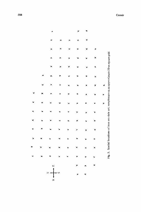
Variogram estimators for iron ore (Table 2), together with number of pairs used in estimating them, are given. Estimated values using (4) are plotted with the best fit superimposed (Fig. 2). A straight line fit on data only up to lag 7 (Fig. 2a) was considered all that was necessary as kriging would not involve points at greater distances (screen effect), and weighted least-squares fitting in the straight line case would automatically mean that greater lags would contribute almost nothing to the weighted sum of squares. The residual variogram estimate, however, shows spherical structure beyond lag 7, and so estimates up to lag 11 were used in the weighted least-squares fit (Fig. 2b). For confidentiality reasons, the iron ore data set cannot be shown in its entirety, but a plan of the spatial locations of the sample (and of course, of the median polish residuals) (Fig. 3) is given.

In summary then, using the method of weighted least-squares, we have been able to estimate variogram values in the following situations:

Table 2. Iron Ore Data

Originals Residuals

h 2~(h) [2~(h)] N h 2~(h) [ 2~(h)] h

1 13.10 (14.39) 103 11.50 (11.96) 1 2 14.81 (18.43) 94 11.89 (13.69) 2 3 14.66 (16.93) 85 11.29 (13.46) 3 4 17.31 (18.67) 77 13.08 (14.05) 4 5 26.50 (23.67) 69 17.38 (16.35) 5 6 19.14 (18.54) 61 14.74 (13.39) 6 7 27.31 (24.66) 53 18.49 (21.96) 7 8 41.65 (33.33) 45 17.86 (23.13) 8 9 36.00 (34.26) 38 16.97 (19.88) 9

10 27.16 (30.15) 31 12.90 (16.64) 10 11 37.37 (39.67) 25 16.31 (19.60) 11 12 39.89 (37.05) 19 15.32 (17.02) 12 13 48.08 (39.03) 13 22.18 (25.49) 13 14 53.18 (48.78) 7 37.90 (25.66) 14 15 165.29 (96.22) 4 19.02 (15.81) 15 16 203.52 (145.44) 2 9.40 (8.80) 16

aE-W direction; originals and residuals (from median polish). Entries show robust variogram estimator (4) (classical variogram estimator 3 is in parentheses), and number of pairsN h involved in the tag h estimator.

27

3 0

25

( a )

20

15

lO

X

582 Cressie

l a g

0 I I ] I I I I IL

1 2 3 4 5 6 7

Fig. 2. (a) Iron ore data; E-W direction; originals. Weighted least-squares fit of straight line variogram to estimated variogram (marked with ×), up to lag 7. (b) Iron ore data; E-W direc- tion; residuals from median polish. Weighted least-squares fit of spherical variogram to esti- mated variogram (marked with ×), up to lag 11.

Coal ash originals, N-S:

Co = 0.89,

Coal ash residuals, N-S:

Co + c s = 0.77,

Iron ore originals, E-W:

Spherical model (24)

c s = 0.14, a s = 4.31

Spherical model (24)

a s = 0 (pure nugget effect)

Linear model (26)

Co = 5.17, b / = 1 . 1 1

Iron ore residuals, E-W: Spherical model (24)

Co = 4.83, cs = 3.59, as = 8.73.

Fitting Vaxioglam Models 583

2~

2 5

1 5

(b)

x

J

lag 0 J I J i I I I I ' J I - I ~

i 2 3 4 5 6 7 8 9 10 11

Fig. 2. Continued

We also tried exponential (see 25) fitting, and in each case the spherical fit im- proved the weighted sums of squares by a few percent.

Before the final model is chosen, one has to take into account variograms in other directions, possible anisotropies, and so forth. These adjustments are usually made however, in light of a first sensible fitting of a model to estimated variogram values. This is why a statistically based approach to variogram estima- tion must be of interest to the practicing geostatistican.

4. CONCLUDING REMARKS

The variable (Z t+ h - Z t ) 2 is v e l T skewed, and 1~ (Z t i - Z t. + h)2 /A~h remains skewed (although less so), whereas Z [Zt i + h - Z t i ] l / 2 / N h has'less of a skewness problem. Weighted least squares, which is Gaussian-based, may not be all that appropriate for small N h. Some other criterion which takes into account the in- herent positiveness and skewness of the estimator would be needed when, say, max { N h ; h >t 1} < 30.

584 Cressie

X

>K

X

X N N "X ~ ~

if3 o

X a

0

e~

M ~ X ~ X ~ N

x x x N x x

M ~ ~ 'X N 0

0

0

><

Fitting Variogram Models 585

In conclusion then, we have tried to formalize the method of variogram model fitt ing by setting out three possible approaches.

(i) Least squares (see 6). This, and "eyeball ing," are probably the methods most used today. David (1977, p. 522) does talk about weighting each variogram estimator according to the number of points involved in estima-

t ion, but does not say how. (ii) Weighted least squares (see 23). This has the desirable feature that weight-

ing is directly proport ional to the number of observations Nh, and is larger for smaller lags.

(iii) Generalized least squares (see 7). A way to handle the forbidding expres-

sions for E, through iteration, is given (Subsection 2.3).

Weighted least squares is the true compromise between simplicity and sta- tistical efficiency. A fit based on the robust estimator (4) needs less compromise than the Matheron estimator (3). We do n o t recommend blind use of this method, but rather recommend it as a way of homing in on a satisfactory model that atso takes into account such things as anisotropies and geological considerations.

ACKNOWLEDGMENT

Comments on a first draft, from Doug Hawkins, Andr6 Journel, and Geoff Laslett, are gratefully acknowledged.

REFERENCES

Armstrong, M., 1984, Improving the estimation and modelling of the variogram, in G. Verly et al. (Eds.) Geostatistics for natural resources characterization: Dordrecht, Reidel, p. 1-19.

Armstrong, M. and Delfiner, P., 1980, Towards a more robust variogram: A case study on coal, Internal note N-671: Centre de Geostatistique, Fontainebleau, France.

Buxton, B., 1982, A geostatisticaI case study, unpublished masters thesis: Stanford Univer- sity, California, 84 p.

Carroll, R.J. and Ruppert, D., 1982, A comparison between maximum likelihood and generalized least squares in a heteroscedastic linear model: Your. Amer. Stat. Assoc., v. 77, p. 878-882.

Clark, I., 1979, Practical geostatistics: Applied Science Publishers, Essex, England, 129 p. Cressie, N. A. C., 1979, Straight line fitting and variogram estimation (with discussion):

Bull. Inter. Stat. Inst., v. 48, Book 3, p. 573-582. Cressie, N. A. C., 1980, M-estimation in the presence of unequal scale. Stat. Neerlandiea, v.

34, p. 19-32. Cressie, N. A. C., 1984, Towards resistant geostatistics, in G. Verley et al. (Eds.) Geostatis-

tics for natural resources characterization: Dordrecht, Reidel, p. 21-44. Cressie, N. A. C. and Glonek, G., 1984, Median based covariogram estimators reduce bias:

Star. Prob. Lett., v. 2, p. 299-304. Cressie, N. A. C. and Hawkins, D.M., 1980, Robust estimation of the variogram: Your.

Inter. Assoc. Math. Geol., v. 12, p. 115-125.

586 Cressie

David, M., 1977, Geostatistical ore reserve estimation: Amsterdam, Elsevier, 364 p. Davis, B. M. and Borgman, L. E., 1982, A note on the asymptotic distribution of the sample

variogram: Jour. Inter. Assoc. Math. Geol., v. 14, p. 189-193. Delfiner, P., 1976, Linear estimation of nonstationary spatial phenomena, in M. Guarascio

et al. (Eds.) Advanced geostatics in the mining industry: Dordrecht, Reidel, p. 49-68. Diamond, P. and Armstrong, M., 1983, Robustness of variograms and conditioning of krig-

ing matrices: Internal note N-804, Centre de Geostatistique, Fontainebleau, France. Gomez, M. and Hazen, K., 1970, Evaluating sulfur and ash distribution in coal seams by sta-

tistical response surface regression analysis: U.S. Bureau of Mines Report, RI 7377. Hawkins, D. M. and Cressie, N. A. C., 1984, Robust kriging-a proposal: Jour. Inter. Assoc.

Math. Geol., v. 16, p. 3-18. Huber, P. J., 1964, Robust estimation of a location parameter: Ann. Math. Stat., v. 35, p.

73-101. Journel, A. and Huijbregts, C., 1978, Mining geostatistics: London, Academic Press, 600 p. King, H. F., McMahon, D. W., and Bujtor, G. J., 1982, A guide to the understanding of ore

reserve estimation, in Proceedings of the Australasian Institute of Mining and MetaUurgy, Supplement: v. 281, p. 1-21.

Matheron, G., 1963, Pfinciples of geostatistics: Econ. Geol., v. 58, p. 1246-1266. Matheron, G., 1971, The theory of regionalized variables and its applications: Cahiers du

Centre de Morphologie Mathematique, No. 5, Fontainebleau, France. Sharp, W. E., 1982, Estimation of semi-variograms by. the maximum entropy method: Jour.

Inter. Assoc. Math. Geol., v. 14, p. 456-474. Starks, T. and Fang, J., 1982a, On the estimation of the generalized covariance function:

Jour. Inter. Assoc. Math. Geol., v. 14, p. 57-64. Starks, T. and Fang, J., 1982b, The effect of drift on the experimental semi-variogram: Jour.

Inter. Assoc. Math. Geol., v. 14, p. 309-320. Switzer, P., 1984, Inference for spatial autocorrelation functions in G. Verly et al. (Eds.)

Geostatistics for natural resources characterization: Dordrecht, Reidel, p. 127-140.