fixed point result in controlled fuzzy metric spaces with

Fixed Point Result in Controlled Fuzzy MetricSpaces with Application to Dynamic MarketEquilibriumRakesh Tiwari

Post Graduate Autonomous Collegevladimir rakocevic ( [email protected] )

Rossijskij universitet druzby narodov Fakul'tet ziko-matematiceskih i estestvennyh naukShraddha Rajput

La Postemous College

Research Article

Keywords: Fixed point, Fuzzy metric spaces, Controlled fuzzy metric spaces, Fuzzy f -contractivemapping, Dynamic market equilibrium

Posted Date: October 25th, 2021

DOI: https://doi.org/10.21203/rs.3.rs-735573/v1

License: This work is licensed under a Creative Commons Attribution 4.0 International License. Read Full License

https://doi.org/10.21203/rs.3.rs-735573/v1

mailto:[email protected]

https://doi.org/10.21203/rs.3.rs-735573/v1

https://creativecommons.org/licenses/by/4.0/

Fixed Point Result in Controlled Fuzzy Metric Spaces

with Application to Dynamic Market Equilibrium

Rakesh Tiwari,1 Vladimir Rakocevic and Shraddha Rajput2

1,2Department of Mathematics, Government V. Y. T. Post-Graduate AutonomousCollege, Durg 491001, Chhattisgarh, India.Email: [email protected], [email protected]∗University of NIS, Faculty of Sciences and Mathematics, Visegradska 33, 18000NIS SerbiaEmail: ∗[email protected]

Abstract. In this paper, inspired by the work of Muzeyyen Sangurlu Sezen [22] and H.Saleh Nasr et al. [20], we introduce Θf -type controlled fuzzy metric spaces and establishsome fixed point results in controlled fuzzy metric spaces. We provide suitable examplesto validate our result. We also employ an application to substantiate the utility of ourestablished result for finding the unique solution of an integral equation emerging in thedynamic market equilibrium aspects to economics.Subject Classification: 54H25, 47H10, A11.Keywords: Fixed point, Fuzzy metric spaces, Controlled fuzzy metric spaces, FuzzyΘf -contractive mapping, Dynamic market equilibrium.

1 Introduction

In 1922, S. Banach [6] provided an important result to the fixed point theory. Thistopic has been studied, presented and generalized by many researchers in many differentspaces. Firstly, the work of Bakhtin [5], Bourbaki [7] and Czerwik [8] expanded thetheory of fixed points for b-metric spaces. Also, many authors proved some importantfixed point theorems in b-metric spaces ([1], [2], [3]). Controlled metric spaces introducedby Nabil Mlaiki et al. [18] and proved some fixed point theorems.

On the other hand, important theoretical development in the fuzzy sets theory in-troduced by Zadeh [25]. Fuzzy sets theory is the way of defining the concept of fuzzymetric spaces by Kramosil and Michalek [14], which can be regarded as a generalizationof the statistical metric spaces. Subsequently, M. Grabiec [11] defined G-complete fuzzymetric spaces and extended the complete fuzzy metric spaces. Following Grabiec’s work,George and Veeramani [10] modified the notion of M -complete fuzzy metric spaces withthe help of continuous t-norms.

Corresponding author

1

2 Fixed Point Result · · · · · · Dynamic Market Equilibrium

Nadaban [19] introduced the concept of fuzzy b-metric spaces. Kim et al. [13] estab-lished some fixed point results in fuzzy b-metric spaces. Recently, Mehmood et al. [15]has defined a new concept called extended fuzzy b-metric spaces, which is the general-ization of fuzzy b-metric spaces. Muzeyyen Sangurlu Sezen [22] introduced controlledfuzzy metric spaces, which is a generalization of extended fuzzy b-metric spaces.

Many authors introduced and generalized the numerous types of fuzzy contractivemappings ([4], [16], [17], [23], [24]) and investigated some fixed point theorems in fuzzymetric spaces. H. Saleh Nasr et al.[20] introduced Fuzzy Θf - contractive mapping es-tablish some fixed point theorems.

2 Preliminaries

Now, we begin with some basic concepts, notations and definitions. Let R representthe set of real numbers, R+ represent the set of all non-negative real numbers and N

represent the set of natural numbers.

We start with the following definitions of a fuzzy metric space.

Definition 2.1. [10]. An ordered triple (X,M, ∗) is called fuzzy metric space such that Xis a nonempty set, ∗ defined a continuous t-norm and M is a fuzzy set on X×X×(0,∞),satisfying the following conditions, for all x, y, z ∈ X, s, t > 0.(FM-1) M(x, y, t) > 0.(FM-2) M(x, y, t) = 1 iff x = y.(FM-3) M(x, y, t) =M(y, x, t).(FM-4) (M(x, y, t) ∗M(y, z, s)) ≤M(x, z, t+ s).(FM-5) M(x, y, ·) : (0,∞) → (0, 1] is left continuous.

In 2017, Nadaban [19] introduced the idea of a fuzzy b-metric space to generalize thenotion of a fuzzy metric spaces introduced by Kramosil and Michalek [14].

Definition 2.2. [19]. Let X is a non-empty set and b ≥ 1 be a given real number and∗ be a continuous t-norm. A fuzzy set M in X2 × (0,∞) is called fuzzy b-metric on Xif for all x, y, z ∈ X and s, t > 0 the following conditions hold.(FbM-1) M(x, y, t) = 0.(FbM-2) M(x, y, t) = 1 iff x = y.(FbM-3) M(x, y, t) =M(y, x, t).(FbM-4) M(x, z, b(t+ s)) ≥M(x, y, t) ∗M(y, z, s).(FbM-5) M(x, y, ·) : (0,∞) → [0, 1] is left continuous and limt→∞M(x, y, t) = 1.

Mehmood et al. [15] introduced the notion of an extended fuzzy b-metric spacefollowing the approach of Grabiec [11].

Definition 2.3. [15]. Let X be a non-empty set, α : X×X → [1,∞), ∗ is a continuoust-norm and Mα is a fuzzy set on X2 × (0,∞), is called extended fuzzy b-metric on X iffor all x, y, z ∈ X and s, t > 0, satisfying the following conditions.

Rakesh Tiwari, Vladimir Rakocevic and Shraddha Rajput 3

(FbMα1) Mα(x, y, 0) = 0.(FbMα2) Mα(x, y, t) = 1 iff x = y.(FbMα3) Mα(x, y, t) =Mα(y, x, t).(FbMα4) Mα(x, z, α(x, z)(t+ s)) ≥Mα(x, y, t) ∗Mα(y, z, s).(FbMα5) Mα(x, y, ·) : (0,∞) → [0, 1] is continuous.Then (X,Mα, ∗, α(x, y)) is an extended fuzzy b-metric space.

In [22], Sezen introduced the controlled fuzzy metric spaces, which is a generalizationof extended fuzzy b-metric spaces.

Definition 2.4. [22]. Let X be a non-empty set, λ : X×X → [1,∞), ∗ is a continuoust-norm and Mλ is a fuzzy set on X2 × (0,∞), satisfying the following conditions, for alla, c, d ∈ X, s, t > 0 :(FM-1) Mλ(a, c, 0) = 0.(FM-2) Mλ(a, c, t) = 1 iff a = c.(FM-3) Mλ(a, c, t) =Mλ(c, a, t).(FM-4) Mλ(a, d, t+ s) ≥Mλ(a, c,

tλ(a,c)

) ∗Mλ(c, d,s

λ(c,d)).

(FM-5) Mλ(a, c, ·) : [0,∞) → [0, 1] is continuous.Then, the triple (X,Mλ, ∗) is called a controlled fuzzy metric space on X.

Definition 2.5. [21]. Let F : X → X and α : X × X → [0,∞). Then F is anα-admissible mapping, if

α(x, y) ≥ 1 ⇒ α(F (x), F (y)) ≥ 1, x, y ∈ X. (2.1)

Definition 2.6. [20]. Θf : (0, 1) → (0, 1), such that Θf is non decreasing continuousand satisfying condition for each sequence βn ⊂ (0, 1),

limn→∞Θf (βn) = 1 ⇔ limn→∞βn = 1. (2.2)

Definition 2.7. [22]. Let (X,Mλ, ∗) be a controlled fuzzy metric spaces. Then

1. A sequence xn in X is said to be G-convergent to x in X, if and only iflimn→∞Mλ(xn, x, t) = 1 for any n > 0 and for all t > 0.

2. A sequence xn in X is said to be G-Cauchy sequence if and only iflimn→∞Mλ(xn, xn+m, t) = 1 for any m > 0 and for all t > 0.

3. The controlled fuzzy metric space is called G-complete if everyG- Cauchy sequence is convergent.

The objective of this work is to prove a Banach type fixed point theorem in controlledfuzzy metric spaces using fuzzy Θf - contractive mapping, which is an extension of [10],[15], [19], [20], [22]. Our result generalizes many recent fixed point theorems in theliterature ([13], [15], [19], [20]). We furnish an example to validate our result. Applicationis also provided to show the utility of our result.


3 Main Result

In this section, we introduce some new definitions and establish a fixed point theoremin controlled fuzzy metric spaces.

Definition 3.1. Let Y be a non-empty set, λ : Y ×Y → [1,∞), ∗ is a continuous t-normand Mλ is a fuzzy set on Y 2 × (0,∞), for all a, c, d ∈ Y, s, t > 0, Θf : [0, 1] → [0, 1],satisfying the following conditions,(ΘfFMλ-1) Θf (Mλ(a, c, 0)) = 0.(ΘfFMλ-2) Θf (Mλ(a, c, t)) = 1 iff a = c.(ΘfFMλ-3) Θf (Mλ((a, c, t)) = Θf (Mλ(c, a, t)).(ΘfFMλ-4) Θf (Mλ(a, d, t+ s)) ≥ Θf (Mλ(a, c,

tλ(a,c)

) ∗Mλ(c, d,s

λ(c,d))).

(ΘfFMλ-5) Θf (Mλ(a, c, ·)) : [0,∞) → [0, 1] is continuous.Then, the triple (Y,ΘfMλ, ∗) is called a Θf -type controlled fuzzy metric spaces on Y.

Now, we display an example to verify our definition.

Example 3.2. Let Y = A ∪ C where A = (0, 2) and C = [2,∞). Define Mλ is a fuzzyset on Y 2 × (0,∞), as

Mλ(a, c, t) =

1 if a = c

e−3

ct if a ∈ A and c ∈ C

e−3

at if a ∈ C and c ∈ A

e−3

t otherwise.

With the continuous t-norm ∗ such that t1 ∗ t2 = t1t2. Taking Θf (β) = e1−1

β and defineλ : Y × Y → [1,∞), as

λ(a, c) =

1 if a, c ∈ A

maxa, c otherwise.

Let us show that (Y,ΘfMλ, ∗) is a Θf - type controlled fuzzy metric space on Y. It is easyto prove conditions (ΘfFMλ-1), (ΘfFMλ-2) and (ΘfFMλ-3). We have to examine thefollowing cases to show that condition (ΘfFMλ-4) holds.Case I. If d = a or d = c, (ΘfFMλ-4) is satisfied.Case II. If d 6= a and d 6= c, (ΘfFMλ-4) holds when a = c.Suppose that a 6= c. Then, we get a 6= c 6= d. Now, we can see that (ΘfFMλ-4) is satisfiedin all the cases below:

1. Let a, c, d ∈ A and a, c, d ∈ C, choose t = 1, s = 1 and a = 1, c = 12, d = 3

2and

λ(a, c) = 1, λ(a, d) = 1, then we get Θf (e−1.5) ≥ Θf (e

−6).

2. Let a, d ∈ A and c ∈ C, choose t = 1, s = 1 and a = 12, c = 3, d = 3

2and

λ(a, c) = maxa, c = 3, λ(a, d) = 32, then we get Θf (e

−0.5) ≥ Θf (e−1).

3. Let a, d ∈ C and c ∈ A, choose t = 1, s = 1 and a = 3, c = 32, d = 4 and

λ(a, c) = maxa, c = 3, λ(a, d) = 1, then we get Θf (e−0.5) ≥ Θf (e

−1.3).


4. Let a ∈ C and c, d ∈ A, choose t = 1, s = 1, and a = 4, c = 12, d = 3

2and


−0.93).

5. Let a, c ∈ A and d ∈ C, choose t = 1, s = 1 and a = 12, c = 3

2, d = 4 and

λ(a, c) = 1, λ(a, d) = 1, then we get Θf (e−1.5) ≥ Θf (e

−6).

6. Let a, c ∈ C and d ∈ A, choose t = 1, s = 1, and a = 3, c = 4, d = 12and


−1.75).

7. Let c, d ∈ C and a ∈ A, choose t = 1, s = 1, and a = 32, c = 3, d = 4 and


−0.6).

Consequently, (Y,ΘfMλ, ∗) is a Θf type controlled fuzzy metric space on X . Also, forthe same functions λ using by (ΘfFMλ-4), we get

Θf (Mλ(a, d, t+ s)) ≥ Θf (Mλ(a, d,t

λ(a, c)) ∗Mλ(c, d,

t

λ(c, d))).

Definition 3.3. Let (Y,ΘfMλ, ∗) is a Θf type controlled fuzzy metric space on X withλ : Y × Y → [1,∞), A mapping S : Y → Y is called a fuzzy Θf weak contractive withrespect to Θf ∈ Ω, and Y is α- admissible. There exist l ∈ (0, 1) such that

Mλ(Sa, Sc, t) < 1 ⇒ α(a, c)Θf (Mλ(Sa, Sc, t)) ≥ [Θf (N(a, c, t))]l (3.1)

for all a, c ∈ Y and t > 0, where

N(a, c, t) = minMλ(a, c, t),Mλ(a, Sa, t),Mλ(c, Sc, t),Mλ(a, Sa, t)Mλ(c, Sc, t)

Mλ(a, c, t). (3.2)

Theorem 3.4. Let (Y,ΘfMλ, ∗) is a Θf type controlled fuzzy metric space on Y. Amapping S : Y → Y is a fuzzy Θf weak contractive and Y is α- admissible, then Sadmits a unique fixed point.

Proof. Let a0 is an arbitrary point in Y,

α(a0, Sa0) ≥ 1.

We define a sequence an in Y by

an+1 = San for all n ∈ N.

Obviously if, there exists n0 ∈ N such that

an0= San0+1,

then San0= an0

and the proof is finished. Suppose that an 6= an+1 for all n ∈ N, thatis, α(Sn, Sn+1) ≥ 1.

Mλ(San−1, San, t) < 1 for all n ∈ N and s > 0.


Using (3.1), since S is a (α,Θf ) type contraction, so for all n ∈ N, we can write

1 > Mλ(San−1, San, t) ⇒ α(an, an+1)Θf (Mλ(San−1, San, t))

≥ [Θf (N(an−1, an, t))]l

≥ [Θf (minMλ(an−1, an, t),Mλ(an−1, an, t),Mλ(an, an+1, t),

Mλ(an−1, an, t)Mλ(an, an+1, t)

Mλ(an−1, an, t))]l

≥ [Θf (minMλ(an−1, an, t),Mλ(an, an+1, t))]l.

Thus

Θf (Mλ(an, an+1, t) ≥ [Θf (minMλ(an−1, an, t),Mλ(an, an+1, t))]l. (3.3)

If there exists n ∈ N such that

minMλ(an−1, an, t),Mλ(an, an+1, t) =Mλ(an, an+1, t),

so

Θf (Mλ(an, an+1, t) ≥ [Θf (Mλ(an, an+1, t))]l > Mλ(an, an+1, t).

Which is contradiction. Therefore

minMλ(an−1, an, t),Mλ(an, an+1, t) =Mλ(an−1, an, t),

so

Θf (Mλ(an, an+1, t) ≥ [Θf (Mλ(an−1, an, t))]l > Mλ(an−1, an, t),

for all n ∈ N. Thus (3.3), we get

Θf (Mλ(an, an+1, t)) ≥ [Θf (Mλ(an−1, an,t

k))]l

≥ [Θ2f (Mλ(an−2, an−1,

t

k2))]l

2

≥ [Θ3f (Mλ(an−3, an−2,

t

k3))]l

3

...

≥ [Θnf (Mλ(a0, a1,

t

kn))]l

n

. (3.4)

Thus by (3.3), we have

≥ [Θf (Mλ(a0, a1,t

kn))]l

n

> Mλ(a0, a1,t

kn). (3.5)


Consider the triangle inequality, using the condition (ΘfFMλ-4), we have

Θf (Mλ(an, an+m, t)) ≥ Θf (Mλ(an, an+1,t

2λ(an, an+1)) ∗Mλ(an+1, an+m,

t

2λ(an+1, an+m)))

≥ Θf (Mλ(an, an+1,t

2λ(an, an+1))

∗Mλ(an+1, an+2,t

(2)2λ(an+1, an+m)λ(an+1, an+2))

∗Mλ(an+2, an+m,t

(2)2λ(an+1, an+m)µ(an+2, an+m)))

≥ Θf (Mλ(an, an+1,t

2λ(an, an+1))

∗Mλ(an+1, an+2,t

(2)2λ(an+1, an+m)λ(an+1, an+2))

∗Mλ(an+2, an+3,t

(2)3λ(an+1, an+m)λ(an+2, an+m)λ(an+2, an+3))

∗Mλ(an+3, an+m,t

(2)3λ(an+1, an+m)λ(an+2, an+m)λ(an+3, an+m)))

...

≥ Θnf (Mλ(a0, a1,

t

2kn−1λ(an, an+1)))

∗ [∗n+m−2i=n+1 Θi

f (Mλ(a0, a1,t

(2)m−1ki−1(∏i

j=n+1 µ(aj, an+m))λ(ai, ai+1))]

∗ [Θn+m−1f (Mλ(a0, a1,

t

(2)m−1kn+m−1(∏n+m−1

i=n+1 µ(ai, an+m)))].

(3.6)

Θf is non decreasing continuous and satisfying condition for each sequence βn ⊂ (0, 1)

limn→∞

Θf (αn) = 1 ⇔ limn→∞

αn = 1. (3.7)

Therefore, by taking limit as n→ ∞ in (3.6), from (3.5) together with (3.1) we have

limn→∞

Θf (Mλ(an, an+m, t)) ≥ (1 ∗ 1 ∗ · · · ∗ 1) = 1,

for all t > 0 and n,m ∈ N. Thus, an is a G-Cauchy sequence in X. From thecompleteness of (X,Mλ, ∗), there exists u ∈ X such that

limn→∞

Mλ(an, u, t) = 1, (3.8)


for all t > 0. Now we show that u is a fixed point of h. For any t > 0 and from thecondition (FMλ-4), we have

Θf (Mλ(u, Su, t)) ≥ Θf (Mλ(u, an+1,t

2λ(an, an+1)) ∗Mλ(an+1, Su,

t

2λ(an+1, Su)))

= Θf (Mλ(u, an+1,t

2λ(u, an+1))

∗Mλ(San, Su,t

2λ(an+1, Su))

≥ Θf (Mλ(u, an+1,t

2λ(u, an+1)))

∗Θf (Mλ(an, u,t

2λ(an+1, Su)). (3.9)

Letting n→ ∞ in (3.9) and using (3.8), we get

limn→∞

Θf (Mλ(u, Su, t)) = 1,

by definition of Θf , we have

limn→∞

Θf (Mλ(u, Su, t)) = 1 ⇔ limn→∞

Mλ(u, Su, t) = 1,

for all t > 0, that is, u = Su.Let w ∈ X is an another fixed point of S and there exists t > 0 such that u 6= w, thenit follows from (3.1) that

Θf (Mλ(u, w, t)) = Θf (Mλ(Su, Sw, t))

≥ Θf (Mλ(u, w,t

k))

≥ Θf (Mλ(u, w,t

k2)

...

> Θf (Mλ(u, w,t

kn), (3.10)

for all n ∈ N. By taking limit as n → ∞ in (3.9), Mλ(u, w, t) = 1 for all t > 0, that is,u = w. This completes the proof.

Remark 3.5. Putting Θf (β) = β, α(a, c) = 1 and


Mλ(a, c, t)

=Mλ(a, c, t)

in Theorem 3.4, we obtain the following result.


Corollary 3.6. Let (Y,ΘfMλ, ∗) is a Θf -type controlled fuzzy metric space on Y. IfS : Y → Y is a mapping such that for all a, c ∈ Y, and λ : Y × Y → [1,∞), t > 0 forsome l ∈ (0, 1)

Mλ(Sa, Sc, t) ≥ [Mλ(a, c, t)]l,

then S admits a unique fixed point.

Remark 3.7. By taking l = 1, in corollary 3.6, we infer the Theorem 2 in [22].

We furnish an example to validate our main result.

Example 3.8. Let Y = A ∪ C where A = 22n : n ∈ N and C = 2. DefineMλ : Y × Y × [0,∞) → [0, 1] as

Mλ(a, c, t) =

1 if a = ct

t+ 1

a

if a ∈ A and c ∈ C

t

t+ 1

c

if a ∈ C and c ∈ A

( tt+1

)1

3 otherwise.

With the continuous t-norm ∗ such that t1 ∗ t2 = t1.t2. Define λ : Y × Y → [1,∞), as

λ(a, c) =

1 if a, c ∈ A

maxa, c otherwise.

Clearly (Y,ΘfFMλ, ∗) is a Θf type controlled fuzzy metric space and we take Θf (β) =β, β ∈ (0, 1], α(a, c) ≥ 1. Consider S : Y → Y by

S(a) =

√2 if a ∈ A

22n+1

if a ∈ C.

Now let us show that (Y,ΘfFMλ, ∗) is a Θf controlled fuzzy metric space. It is easyto prove conditions (ΘfFMλ-1), (ΘfFMλ-2) and (ΘfFMλ-3). We have to examine thefollowing cases to show that condition (ΘfFMλ-4) holds.Case I. If a = c then we have Sa = Sc. In this case:

Θf (Mλ(Sa, Sc, t)) = 1 = Θf (Nλ(a, c, t))1

2 .

Case II. Let a ∈ A and c ∈ C, then we have Sa ∈ A and Sc ∈ C. In this case:

Θf (Mλ(Sa, Sc, t)) = Θf (t

(t+ 1S(a)

))

= Θf (t

(t+ 1

22n+1 ))

≥ Θf [t

(t+ 122

n )]1

2

= Θf [N(a, c, t)]l. (3.11)


Value of n

1 2 3 4 5 6 7 8 9

0.5

0.6

0.7

0.8

0.9

1

For t =1

L.H.S

R.H.S

108

6

Value of t

42

00

2

Value of n

4

6

8

0.4

1

0.8

0.6

10

L.H.S

R.H.S

Figure 1: Variation of L.H.S = Θf (Mλ(Sa, Sc, t)) with R.H.S = Θf [N(a, c, t)]l ofExample 3.8, case-II on 2D and 3D view, for:(a)Θf (Mλ(Sa, Sc, t)) vs Θf [N(a, c, t)]l at t, n ∈ (1, 10).

Table 1 and 2 show the variation between Θf (Mλ(Sa, Sc, t)) and Θf [N(a, c, t)]l as afunction of n with relative to t. This table justifies inequality (3.11), which observed inboth the curves for the value of t is a higher than 50 as a function of n.

Value of t Value of n Θf (Mλ(Sa, Sc, t)) Θf [N(a, c, t)]l

1 1 0.9412 0.40002 0.9961 0.47065 1 0.500010 1 0.5000

50 1 0.9988 0.49752 0.9999 0.499420 1.0000 0.500050 1.0000 0.5000

Table 1: Variation of Θf (Mλ(Sa, Sc, t)) with Θf [N(a, c, t)]l of inequality (3.11), as afunction of n with fixed value of t = 1 and t = 50.

Value of n Value of t Θf (Mλ(Sa, Sc, t)) Θf [N(a, c, t)]l

1 1 0.9412 0.40002 0.9697 0.444450 0.9988 0.4975100 0.9994 0.4988

50 1 1.000 0.50002 1.000 0.500050 1.000 0.5000100 1.000 0.5000

Table 2: Variation of Θf (Mλ(Sa, Sc, t)) with Θf [N(a, c, t)]l of inequality (3.11) as afunction of n with fixed value of n = 1 and n = 50.


Case III. Let a ∈ C and c ∈ A, then we have Sa ∈ C and Sc ∈ A. In this case:


(t+ 1S(c)

))

= Θf (t

(t+ 1

22n+1 )

)

≥ Θf [t

(t+ 122n

)]1

2

= Θf [N(a, c, t)]l.

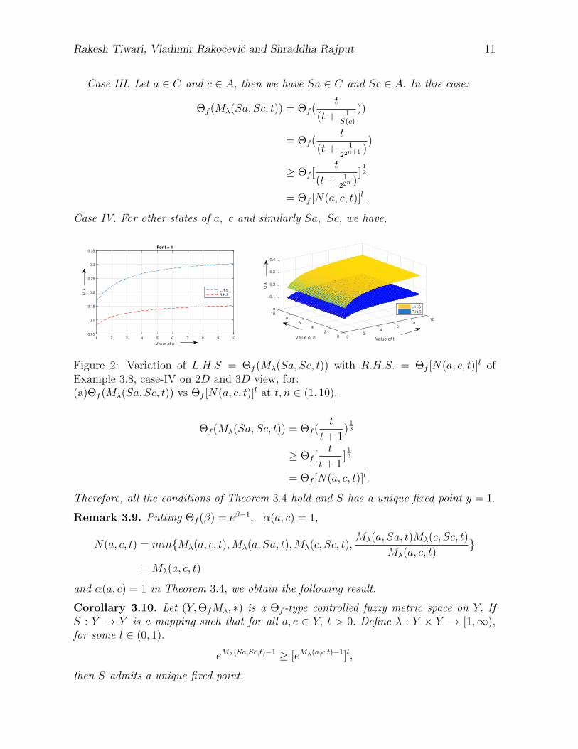
Case IV. For other states of a, c and similarly Sa, Sc, we have,

Value of n

1 2 3 4 5 6 7 8 9 10

0.05

0.1

0.15

0.2

0.25

0.3

0.35For t = 1

L.H.S

R.H.S

108

6

Value of t

42

00

2

Value of n

4

6

8

0.2

0.3

0.4

0

0.1

10

L.H.S

R.H.S

Figure 2: Variation of L.H.S = Θf (Mλ(Sa, Sc, t)) with R.H.S. = Θf [N(a, c, t)]l ofExample 3.8, case-IV on 2D and 3D view, for:(a)Θf (Mλ(Sa, Sc, t)) vs Θf [N(a, c, t)]l at t, n ∈ (1, 10).


t+ 1)1

3

≥ Θf [t

t+ 1]1

6

= Θf [N(a, c, t)]l.

Therefore, all the conditions of Theorem 3.4 hold and S has a unique fixed point y = 1.

Remark 3.9. Putting Θf (β) = eβ−1, α(a, c) = 1,


Mλ(a, c, t)

=Mλ(a, c, t)

and α(a, c) = 1 in Theorem 3.4, we obtain the following result.

Corollary 3.10. Let (Y,ΘfMλ, ∗) is a Θf -type controlled fuzzy metric space on Y. IfS : Y → Y is a mapping such that for all a, c ∈ Y, t > 0. Define λ : Y × Y → [1,∞),for some l ∈ (0, 1).

eMλ(Sa,Sc,t)−1 ≥ [eMλ(a,c,t)−1]l,

then S admits a unique fixed point.


Similarly, by choosing different values of Θf (β), we can obtain several results in theliterature.

4 Application

We also provide an application to substantiate the utility of our established result to findthe unique solution of an integral equation appearing in the dynamic market equilibriumaspects to economics.

Supply Qs and demand Qd are influenced by current prices and price trends (i.e.,whether prices are rising or falling and whether they are rising or falling at an increasingor decreasing rate) in many markets [9]. The economist, therefore, needs to know the

current price P (t), the first derivative dP (t)dt, and the second derivative d2P (t)

dt2. Assume

Qs = g1 + u1P (t) + e1dP (t)

dt+ c1

d2P (t)

dt2

Qd = g2 + u2P (t) + e2dP (t)

dt+ c2

d2P (t)

dt2.

g1, g2, u1, u2, e1 and e2 are constants. Comment on the dynamic stability of the market,if price clears the market at each point in time. In equilibrium, Qs = Qd. Therefore,

g1 + u1P (t) + e1dP (t)

dt+ c1

d2P (t)

dt2= g2 + u2P (t) + e2

dP (t)

dt+ c2

d2P (t)

dt2

since

(c1 − c2)d2P (t)

dt2+ (e1 − e2)d

dP (t)

dt+ (u1 − u2)P (t) = −(g1 − g2).

Letting c = c1 − c2, e = e1 − e2, u = u1 − u2 and g = g1 − g2 in above, we have

cd2P (t)

dt2+ e

dP (t)

dt+ uP (t) = −g,

dividing through by c, P (t) is governed by the following initial value problem

P′′

+ ecP

′

+ ucP (t) = −g

c

P (0) = 0

P ′(0) = 0,

(4.1)

where e2

c= 4u

cand u

e= µ is a continuous function. It is easy to show that the problem

(4.1) is equivalent to the integral equation:

P (t) =

∫ T

0

ζ(t, r)F (t, r, P (r))dr. (4.2)


where ζ(t, r) is Green’s function given by

ζ(t, r) =

reµ2(t−r) if 0 ≤ r ≤ t ≤ T

teµ2(r−t) if 0 ≤ t ≤ r ≤ T.

(4.3)

In this section, by using Corollary 3.6, we will show the existence of a solution to theintegral equation:

P (t) =

∫ T

0

G(t, r, P (r))dr. (4.4)

Let X = C([0, T ]) be the set of real continuous functions defined on [0, T ] . For t > 0,we define

Mλ(a, c, t) = supt∈[0,T ]mina, c+ t

maxa, c+ t(4.5)

for all a, c ∈ Y, with the continuous t-norm ∗ such that t1 ∗ t2 = t1t2. Taking Θf (β) = βand define λ : Y × Y → [1,∞), as

λ(a, c) =

1 if a, c ∈ A

maxa, c otherwise.

It is easy to prove that (Y,Mλ, ∗) is a controlled fuzzy metric spaces. Consider themapping S : Y → Y defined by

SP (t) =

∫ T

0

G(t, r, P (r))dr. (4.6)

Theorem 4.1. Consider equation (4.4) and suppose that

1. G : [0, T ]× [0, T ] → R+ is continuous function,

2. There exist a continuous function ζ : [0, T ]× [0, T ] → R+ such that

supt∈[0,T ]

∫ T

0ζ(t, r)dr ≥ 1,

3. maxG(t, r, a(r))−G(t, r, c(r)) ≥ ζ(t, r)maxa(r), c(r),and minG(t, r, a(r))−G(t, r, c(r)) ≥ ζ(t, r)mina(r), c(r),

4. maxa(r), c(r)+ t ≥ (maxa(r), c(r)+ t)l,and mina(r), c(r)+ t ≥ (mina(r), c(r)+ t)l,

for all l ∈ (0, 1). Then, the integral equation (4.4) has a unique solution.

Proof. For a, c ∈ Y , by using of assumptions (1)–(4), we have


Mλ(Sa, Sc, t) = supt∈[0,T ]

min∫ T

0G(t, r, a(r))dr,

∫ T

0G(t, r, c(r))dr.)+ t

max∫ T

0G(t, r, a(r))dr,

∫ T

0G(t, r, c(r))dr.)+ t

= supt∈[0,T ]

∫ T

0minG(t, r, a(r), G(t, r, c(r))dr + t

∫ T

0maxG(t, r, a(r))dr,G(t, r, c(r))dr + t

≥ supt∈[0,T ]

∫ T

0ζ(t, r)mina(r), c(r)dr + t

∫ T

0ζ(t, r)maxa(r), c(r)dr + t

≥ supt∈[0,T ]

mina(r), c(r)∫ T

0ζ(t, r)dr + t

maxa(r), c(r))∫ T

0ζ(t, r)dr + t

≥ (mina(r), c(r)+ t)l

(maxa(r), c(r))+ t)l

≥ (mina(r), c(r)+ t

maxa(r), c(r))+ t)l

≥ (Mλ(a, c, t))l.

Therefore all the conditions of Corollary 3.6 are satisfied. As a result, the mapping Shas a unique fixed point y ∈ Y, which is a solution of the integral equation (4.4).

Conclusions. In this article, motivated and inspired by the work of Muzeyyen Sangurlu

Sezen [22] and H. Saleh Nasr et al. [20], we generalize the controlled fuzzy metric spaces using

fuzzy Θf - contractive mapping. We obtain a fixed point result by using generalized contractive

conditions in the framework of controlled fuzzy metric spaces. Our investigations and results

obtained were supported by suitable examples. We also provide an application of our result to

the existence of a solution to an integral equation, which determine dynamic market equilibrium

aspects to economics problems. This work provides a new path for researchers in the concerned

field.

Funding: Not applicable.Conflicts of interest/Competing interests: Not applicable.Availability of data and material: Not applicable.Code availability: Not applicable.Authors’ contributions: All the authors contributed equally.

References

[1] Afshari H., Atapour M. and Aydi H., A common fixed point for weak φ - con-tractions on b-metric spaces, Fixed Point Theory, 13(2012), 337 − 346. URL: http ://www.math.ubbcluj.ro/ nodeacj/sfptcj.html.

[2] Afshari H., Atapour M. and Aydi H., Generalized α − ψ−Geraghty multival-ued mappings on b-metric spaces endowed with a graph, J. Appl. Eng. Math.,7(2017), 248− 260.


[3] Afshari H., Atapour M. and Aydi H., Nemytzki-Edelstein-Meir-Keeler type resultsin b-metric spaces, Discret. Dyn. Nat. Soc., (2018), 4745764.

[4] Alharbi N., Aydi H., Felhi A., Ozel C. and Sahmim S., α-Contractive mappings onrectangular b-metric spaces and an application to integral equations, J. Math. Anal.,9(2018), 47− 60.

[5] Bakhtin I. A., The contraction mapping principle in almost metric spaces, Funct.Anal., 30(1989), 26− 37.

[6] Banach S., Sur les operations dans les ensembles abstraits et leur applica-tion aux equations integrals, Fundam. Math., 3(1922), 133 − 181. URL: http ://matwbn.icm.edu.pl/ksiazki/or/or2/or215.pdf.

[7] Boriceanu M., Petrusel A. and Rus I. A., Fixed point theorems for some multivaluedgeneralized contraction in b-metric spaces, Int. J. Math. Statistics, 6(2010), 65− 76.

[8] Czerwik S., Contraction mappings in b-metric spaces, Acta Math. Inform. Univ.Ostra., 1(1993), 5− 11. URL: http : //dml.cz/dmlcz/120469.

[9] Dowling Edward T., Schaum’s Outline Series, Introduction to mathematical eco-nomics, (2001), ISBN: 978 − 0 − 07 − 135896 − 5. link: www.rhayden.uspartial −derivatives− 2economic− applications− jpw.html.

[10] George A. and Veeramani P., On some results in fuzzy metric spaces, Fuzzy Setsand Systems, 64(1994), 395− 399. DOI:10.1016/0165− 0114(94)90162− 7.

[11] Grabiec M., Fixed points in fuzzy metric spaces, Fuzzy Sets and Systems,27(1988), 385− 389. DOI:10.1016/0165− 0114(88)90064− 4.

[12] Hao Y. and Guan Hongyan, On Some Common Fixed Point Results for Weakly Con-traction Mappings with Application, Journal of Function Spaces, 2021(2021), 5573983.DOI :10.1155/2021/5573983.

[13] Kim J. K., Common fixed point theorems for non-compatible self-mappings in b-fuzzy metric spaces, J. Computational Anal. Appl., 22(2017), 336− 345.

[14] Kramosil I. and Michalek J., Fuzzy metric and statistical metric spaces, Kyber-netika, 11(1975), 326− 334. URL: http : //dml.cz/dmlcz/125556.

[15] Mehmood F., Ali R., Ionescu C. and Kamran T., Extended fuzzy b-metric spaces,J. Math. Anal., 8(2017), 124− 131. URL: http : //www.ilirias.com.

[16] Melliani S., and Moussaoui A., Fixed point theorem using a new class of fuzzycontractive mappings, Journal of Universal Mathematics, 1(2)(2018), 148− 154.

[17] Mihet D., Fuzzy ψ-contractive mappings in non-archimedean fuzzy metric spaces,Fuzzy Sets and Systems, 159(6)(2008), 739− 744. DOI:10.1016/j.fss.2007.07.006.


[18] Mlaiki N., Aydi H., Souayah N. and Abdeljawad T., Controlled metric type spacesand the related contraction principle, Mathematics Molecular Diversity PreservationInternational, 6(2018), 1− 7. DOI:10.3390/math6100194.

[19] Nadaban S., Fuzzy b-metric spaces, Int. J. Comput. Commun. Control,11(2016), 273− 281. DOI: 10.15837/ijccc.2016.2.2443.

[20] Nasr Saleh H., Imdad M., Khan I. and Hasanuzzaman M. . Fuzzy Θf -contractivemappings and their fixed points with applications. Journal of Intelligent FuzzySystems,(2020), 1− 10. DOI:10.3233/jifs− 200319.

[21] Samet B., Vetro C. and Vetro P., Fixed point theorems for α−ψ−contractive typemappings, Nonlinear Analysis 75(2012), 2154− 2165. DOI:10.1016/j.na.2011.10.014.

[22] Sezen Muzeyyen Sangurlu, Controlled fuzzy metric spaces and some relatedfixed point results, Numerical Partial Differential Equations, (2020), 1 − 11.DOI:10.1002/num.22541.

[23] Shukla S., Gopal D. and Sintunavarat W., A new class of fuzzy contractivemappings and fixed point theorems, Fuzzy Sets and Systems 350(2018), 85 − 94.DOI:10.1016/j.fss.2018.02.010.

[24] Wardowski D., Fuzzy contractive mappings and fixed points in fuzzy metric spaces,Fuzzy Sets and Systems 222(2013), 108− 114. DOI: 10.1016/j.fss.2013.01.012.

[25] Zadeh L. A., Fuzzy sets, Inform and Control, 8(1965), 338− 353. DOI:10.1016/S0019− 9958(65)90241−X.

fixed point result in controlled fuzzy metric spaces with

Documents