flash user’s guide - university of...
TRANSCRIPT
FLASH User’s GuideVersion 2.5
February 2005
ASC FLASH CenterUniversity of Chicago


0.1. ACKNOWLEDGMENTS IN PUBLICATION i
License
0.1 Acknowledgments in Publication
All publications resulting from the use of the FLASH Code must acknowledge the ASC/Alliance Center for As-trophysical Thermonuclear Flashes. Addition of the following text to the paper acknowledgments will be sufficient.
"The software used in this work was in part developed by the DOE-supported ASC/Alliance Center for Astrophys-ical Thermonuclear Flashes at the University of Chicago."
This is a summary of the rules governing the dissemination of the "Flash Code" by the ASC/Alliances Center forAstrophysical Thermonuclear Flashes (Flash Center) to users outside the Center, and constitutes the License Agree-ment for users of the Flash Code. Users are responsible for following all of the applicable rules described below.
0.2 Full License Agreement
• Public release. We expect to be able to publically release versions of the Flash Code via the Center’s web site,and expect to release any given version of the Flash Code within a year of its formal deposition in the Center’scode archive.
• Decision process. At present, release of the Flash Code to users not located at the University of Chicago orat Argonne National Laboratory is governed soley by the Director and the Management Committee; decisionsrelated to public release of the Flash Code will be made in the same manner.
• Distribution rights. The Flash Code, and any part of this code, can only be released and distributed by the FlashCenter; individual users of the code are not free to re-distribute the Flash Code, or any of its components, outsidethe Center. While the Flash Code is currently not export-controlled, we are nevertheless required to insure thatwe identify all users of this code. For this reason, we require that all users sign a hardcopy version of thisLicense Agreement, and send it to the Flash Center. Distribution of the Flash Code can only occur once a signedLicense Agreement is received by us.
• Modifications and Acknowledgments. You may make modifications to the Flash Code, and we encourage youto send such modifications to the Center; as noted in 3. above, you are not free to distribute this code to others.As resources permit, we plan to incorporate such modifications in subsequent releases of the Flash Code, andwe will acknowledge your contributions. Note that modifications that do not make it into an officially-releasedversion of Flash will not be supported by us.
If you do modify a copy or copies of the Flash Code or any portion of it, thus forming a work based on the FlashCode, you must meet the following conditions:
– a) The software must carry prominent notices stating that you changed specified portions of the FlashCode. This will assist us in clearly identifying the portions of the code that you have contributed.
– b) The software must display the following acknowledgement: "This product includes software developedby and/or derived from the ASC/Alliances Center for Astrophysical Thermonuclear Flashes (http://flash.uchicago.edu)to which the U.S. Government retains certain rights."
– c) The present code header section, describing the origins of the Flash Code and of its components, mustremain intact, and should be included in all modified versions of the code. Furthermore, all publicationsresulting from the use of the Flash Code, or any modified version or portion of the Flash Code, must ac-knowledge the ASC/Alliances Center for Astrophysical Thermonuclear Flashes; addition of the followingtext to the paper acknowledgments will be sufficient: "The software used in this work was in part developedby the DOE- supported ASC/Alliances Center for Astrophysical Thermonuclear Flashes at the University

ii
of Chicago." The code header provides information on various software that has been utilized as part of theFlash development effort (such as the AMR), as well as updated information on the key scientific journalreferences for the Flash Code. We request that such references be included in the reference section of anypapers based on the Flash Code. 5. Commercial use. All users interested in commercial use of the FlashCode must obtain prior written approval from the director of the Flash Center. Use of the Flash Code, orany modification thereof, for commercial purposes is not permitted otherwise.
• Bug fixes and new releases. As part of the code dissemination process, the Center has set up and will maintainas part of its web site mechanisms for announcing new code releases, for collecting requests for code use, andfor collecting and disseminating frequently asked questions (FAQs). We do not plan to provide direct technicalsupport, however, we do support a list ([email protected]) for discussion of user’s questions. Thereis also a list ([email protected]) for reporting the bugs. .
• Use feedback. The Center requests that all users of the Flash Code notify the Center about all publications thatincorporate results based on the use of this code, or modified versions of this code or its components. All suchinformation can be posted on the Center’s web site, at http://flash.uchicago.edu.
• The Flash Code was prepared, in part, as an account of work sponsored by an agency of the United States Gov-ernment. Neither the United States, nor the University of Chicago, nor any contributors to the Flash Code, norany of their employees, makes any warranty, express or implied, or assumes any legal liability or responsibilityfor the accuracy, completeness, or usefulness of any information, apparatus, product, or process disclosed, orrepresents that its use would not infringe privately owned rights.
• IN NO EVENT WILL THE UNITED STATES, THE UNIVERSITY OF CHICAGO OR ANY CONTRIB-UTORS TO THE FLASH CODE BE LIABLE FOR ANY DAMAGES, INCLUDING DIRECT, INCIDEN-TAL, SPECIAL, OR CONSEQUENTIAL DAMAGES RESULTING FROM EXERCISE OF THIS LICENSEAGREEMENT OR THE USE OF THE SOFTWARE.

0.2. FULL LICENSE AGREEMENT iii
Acknowledgments
The FLASH Code Group is supported by the ASC FLASH Center at the University of Chicago under U. S.Department of Energy contract B341495. Some of the test calculations described here were performed on machinesat LLNL, LANL and San Diego Supercomputing Center.
Considerable external and past contributors include:
Alvaro Caceres, Jonathan Dursi, Wolfgang Freis, Bruce Fryxell, Timur Linde, Andrea Mignone, Salvatore Or-lando, Kim Robinson, Paul Ricker, Andrew Siegel, Frank Timmes, Natalia Vladimirova, Greg Weirs, Mike Zingale
PARAMESH was developed under NASA Contracts/Grants NAG5-2652 with George Mason University; NAS5-32350 with Raytheon/STX; NAG5-6029 and NAG5-10026 with Drexel University; NAG5-9016 with the University ofChicago; and NCC5-494 with the GEST Institute. For information on PARAMESH please contact its main developers;Peter MacNeice ([email protected]) or Kevin Olson ([email protected]).

Contents
0.1 Acknowledgments in Publication . . . . . . . . . . . . . . . . . . . . . . . . . . . . . . . . . . . . . i0.2 Full License Agreement . . . . . . . . . . . . . . . . . . . . . . . . . . . . . . . . . . . . . . . . . . i
I Getting Started 1
1 Introduction 31.1 What’s new in FLASH 2.5 . . . . . . . . . . . . . . . . . . . . . . . . . . . . . . . . . . . . . . . . 31.2 About the user’s guide . . . . . . . . . . . . . . . . . . . . . . . . . . . . . . . . . . . . . . . . . . 4
2 Quick start 52.1 System requirements . . . . . . . . . . . . . . . . . . . . . . . . . . . . . . . . . . . . . . . . . . . 52.2 Unpacking and configuring FLASH for quick start . . . . . . . . . . . . . . . . . . . . . . . . . . . 62.3 Running FLASH . . . . . . . . . . . . . . . . . . . . . . . . . . . . . . . . . . . . . . . . . . . . . 8
3 The FLASH configuration script (setup) 11
4 Setting up new problems 154.1 Creating a Config file . . . . . . . . . . . . . . . . . . . . . . . . . . . . . . . . . . . . . . . . . . 154.2 Creating an init_block.F90 . . . . . . . . . . . . . . . . . . . . . . . . . . . . . . . . . . . . . . 164.3 The runtime parameter file (flash.par) . . . . . . . . . . . . . . . . . . . . . . . . . . . . . . . . . 23
II Structure and Modules 27
5 Overview of FLASH architecture 295.1 Structure of a FLASH module . . . . . . . . . . . . . . . . . . . . . . . . . . . . . . . . . . . . . . 29
5.1.1 Configuration layer . . . . . . . . . . . . . . . . . . . . . . . . . . . . . . . . . . . . . . . . 295.1.2 Interface layer and database module . . . . . . . . . . . . . . . . . . . . . . . . . . . . . . . 315.1.3 Algorithms . . . . . . . . . . . . . . . . . . . . . . . . . . . . . . . . . . . . . . . . . . . . 42
5.2 The FLASH source tree . . . . . . . . . . . . . . . . . . . . . . . . . . . . . . . . . . . . . . . . . . 435.2.1 Code infrastructure . . . . . . . . . . . . . . . . . . . . . . . . . . . . . . . . . . . . . . . . 43
5.3 Modules included with FLASH: a brief overview . . . . . . . . . . . . . . . . . . . . . . . . . . . . 45
6 Driver modules 476.1 Delta-formulation and Strang-state driver modules . . . . . . . . . . . . . . . . . . . . . . . . . . . . 49
6.1.1 The euler1 module . . . . . . . . . . . . . . . . . . . . . . . . . . . . . . . . . . . . . . . 506.1.2 The rk3 module . . . . . . . . . . . . . . . . . . . . . . . . . . . . . . . . . . . . . . . . . 506.1.3 strang_state and strang_delta modules . . . . . . . . . . . . . . . . . . . . . . . . . . 516.1.4 The formulation modules . . . . . . . . . . . . . . . . . . . . . . . . . . . . . . . . . . . 52
6.2 Simulation services . . . . . . . . . . . . . . . . . . . . . . . . . . . . . . . . . . . . . . . . . . . . 546.2.1 Runtime parameters . . . . . . . . . . . . . . . . . . . . . . . . . . . . . . . . . . . . . . . 546.2.2 Physical constants . . . . . . . . . . . . . . . . . . . . . . . . . . . . . . . . . . . . . . . . 55
v
vi CONTENTS
7 I/O modules and output formats 577.1 General parameters . . . . . . . . . . . . . . . . . . . . . . . . . . . . . . . . . . . . . . . . . . . . 59
7.1.1 Output file names . . . . . . . . . . . . . . . . . . . . . . . . . . . . . . . . . . . . . . . . . 607.2 Restarting a simulation . . . . . . . . . . . . . . . . . . . . . . . . . . . . . . . . . . . . . . . . . . 617.3 Output formats . . . . . . . . . . . . . . . . . . . . . . . . . . . . . . . . . . . . . . . . . . . . . . 62
7.3.1 HDF5 . . . . . . . . . . . . . . . . . . . . . . . . . . . . . . . . . . . . . . . . . . . . . . . 627.3.2 Parallel-NetCDF . . . . . . . . . . . . . . . . . . . . . . . . . . . . . . . . . . . . . . . . . 657.3.3 HDF4 (Deprecated) . . . . . . . . . . . . . . . . . . . . . . . . . . . . . . . . . . . . . . . . 66
7.4 IO Converter . . . . . . . . . . . . . . . . . . . . . . . . . . . . . . . . . . . . . . . . . . . . . . . 707.5 Working with output files . . . . . . . . . . . . . . . . . . . . . . . . . . . . . . . . . . . . . . . . . 707.6 User-defined variables . . . . . . . . . . . . . . . . . . . . . . . . . . . . . . . . . . . . . . . . . . 70
8 Mesh module 718.1 Introduction . . . . . . . . . . . . . . . . . . . . . . . . . . . . . . . . . . . . . . . . . . . . . . . . 718.2 Specifying the computational domain . . . . . . . . . . . . . . . . . . . . . . . . . . . . . . . . . . 728.3 Mesh geometry . . . . . . . . . . . . . . . . . . . . . . . . . . . . . . . . . . . . . . . . . . . . . . 72
8.3.1 dBase support . . . . . . . . . . . . . . . . . . . . . . . . . . . . . . . . . . . . . . . . . . 728.4 Boundary conditions . . . . . . . . . . . . . . . . . . . . . . . . . . . . . . . . . . . . . . . . . . . 748.5 Adaptive mesh . . . . . . . . . . . . . . . . . . . . . . . . . . . . . . . . . . . . . . . . . . . . . . 75
8.5.1 Introduction . . . . . . . . . . . . . . . . . . . . . . . . . . . . . . . . . . . . . . . . . . . . 758.5.2 Algorithm . . . . . . . . . . . . . . . . . . . . . . . . . . . . . . . . . . . . . . . . . . . . . 758.5.3 Usage . . . . . . . . . . . . . . . . . . . . . . . . . . . . . . . . . . . . . . . . . . . . . . . 758.5.4 Choice of grid geometry . . . . . . . . . . . . . . . . . . . . . . . . . . . . . . . . . . . . . 798.5.5 Using a single-level grid in PARAMESH . . . . . . . . . . . . . . . . . . . . . . . . . . . . 818.5.6 Modifying the refinement criteria with MarkRefLib . . . . . . . . . . . . . . . . . . . . . . . 82
9 Hydrodynamics modules 859.1 The piecewise-parabolic method (PPM) . . . . . . . . . . . . . . . . . . . . . . . . . . . . . . . . . 88
9.1.1 Algorithm . . . . . . . . . . . . . . . . . . . . . . . . . . . . . . . . . . . . . . . . . . . . . 889.1.2 Usage . . . . . . . . . . . . . . . . . . . . . . . . . . . . . . . . . . . . . . . . . . . . . . . 899.1.3 Diffusion . . . . . . . . . . . . . . . . . . . . . . . . . . . . . . . . . . . . . . . . . . . . . 89
9.2 The Kurganov hydrodynamics module . . . . . . . . . . . . . . . . . . . . . . . . . . . . . . . . . . 909.2.1 Algorithm . . . . . . . . . . . . . . . . . . . . . . . . . . . . . . . . . . . . . . . . . . . . . 909.2.2 Usage . . . . . . . . . . . . . . . . . . . . . . . . . . . . . . . . . . . . . . . . . . . . . . . 92
9.3 The Relativistic Hydrodynamics (RHD) Module . . . . . . . . . . . . . . . . . . . . . . . . . . . . . 939.3.1 Overview . . . . . . . . . . . . . . . . . . . . . . . . . . . . . . . . . . . . . . . . . . . . . 939.3.2 Equations . . . . . . . . . . . . . . . . . . . . . . . . . . . . . . . . . . . . . . . . . . . . . 939.3.3 Directory Structure . . . . . . . . . . . . . . . . . . . . . . . . . . . . . . . . . . . . . . . . 949.3.4 Numerical Method . . . . . . . . . . . . . . . . . . . . . . . . . . . . . . . . . . . . . . . . 95
9.4 The magnetohydrodynamics module . . . . . . . . . . . . . . . . . . . . . . . . . . . . . . . . . . . 969.4.1 Description . . . . . . . . . . . . . . . . . . . . . . . . . . . . . . . . . . . . . . . . . . . . 969.4.2 Algorithm . . . . . . . . . . . . . . . . . . . . . . . . . . . . . . . . . . . . . . . . . . . . . 969.4.3 Non-ideal MHD . . . . . . . . . . . . . . . . . . . . . . . . . . . . . . . . . . . . . . . . . 98
10 Material properties modules 9910.1 The multifluid database . . . . . . . . . . . . . . . . . . . . . . . . . . . . . . . . . . . . . . . . . . 10010.2 Equations of state . . . . . . . . . . . . . . . . . . . . . . . . . . . . . . . . . . . . . . . . . . . . . 101
10.2.1 Algorithm . . . . . . . . . . . . . . . . . . . . . . . . . . . . . . . . . . . . . . . . . . . . . 10210.2.2 Usage . . . . . . . . . . . . . . . . . . . . . . . . . . . . . . . . . . . . . . . . . . . . . . . 104
10.3 Compositions . . . . . . . . . . . . . . . . . . . . . . . . . . . . . . . . . . . . . . . . . . . . . . . 10610.3.1 Fuel plus ash mixture (fuel+ash) . . . . . . . . . . . . . . . . . . . . . . . . . . . . . . . . 10710.3.2 Minimal seven-isotope alpha-chain model (iso7) . . . . . . . . . . . . . . . . . . . . . . . . 10710.3.3 Thirteen-isotope alpha-chain model (aprox13) . . . . . . . . . . . . . . . . . . . . . . . . . 10810.3.4 Nineteen-isotope alpha-chain model (aprox19) . . . . . . . . . . . . . . . . . . . . . . . . . 108
CONTENTS vii
10.3.5 Proton-proton/CNO network model (ppcno) . . . . . . . . . . . . . . . . . . . . . . . . . . . 10910.3.6 Proton-electron plasma composition (prot+elec) . . . . . . . . . . . . . . . . . . . . . . . 10910.3.7 Multi-ion plasma composition (ioniz) . . . . . . . . . . . . . . . . . . . . . . . . . . . . . 109
10.4 Thermal conductivity . . . . . . . . . . . . . . . . . . . . . . . . . . . . . . . . . . . . . . . . . . . 11010.4.1 Stellar thermal conductivity . . . . . . . . . . . . . . . . . . . . . . . . . . . . . . . . . . . 11010.4.2 Spitzer thermal conductivity . . . . . . . . . . . . . . . . . . . . . . . . . . . . . . . . . . . 111
10.5 Viscosity . . . . . . . . . . . . . . . . . . . . . . . . . . . . . . . . . . . . . . . . . . . . . . . . . 11110.5.1 Spitzer viscosity . . . . . . . . . . . . . . . . . . . . . . . . . . . . . . . . . . . . . . . . . 111
10.6 Magnetic resistivity and viscosity . . . . . . . . . . . . . . . . . . . . . . . . . . . . . . . . . . . . . 11110.6.1 Constant resistivity . . . . . . . . . . . . . . . . . . . . . . . . . . . . . . . . . . . . . . . . 11110.6.2 Spitzer resistivity . . . . . . . . . . . . . . . . . . . . . . . . . . . . . . . . . . . . . . . . . 111
11 Local source terms 11311.1 The nuclear burning module . . . . . . . . . . . . . . . . . . . . . . . . . . . . . . . . . . . . . . . 113
11.1.1 Detecting shocks . . . . . . . . . . . . . . . . . . . . . . . . . . . . . . . . . . . . . . . . . 11411.1.2 Algorithms . . . . . . . . . . . . . . . . . . . . . . . . . . . . . . . . . . . . . . . . . . . . 11411.1.3 Energy generation rates and reaction rates . . . . . . . . . . . . . . . . . . . . . . . . . . . . 118
11.2 Ionization . . . . . . . . . . . . . . . . . . . . . . . . . . . . . . . . . . . . . . . . . . . . . . . . . 11911.2.1 Algorithms . . . . . . . . . . . . . . . . . . . . . . . . . . . . . . . . . . . . . . . . . . . . 12011.2.2 Usage . . . . . . . . . . . . . . . . . . . . . . . . . . . . . . . . . . . . . . . . . . . . . . . 120
11.3 Stirring . . . . . . . . . . . . . . . . . . . . . . . . . . . . . . . . . . . . . . . . . . . . . . . . . . 12111.4 Heating . . . . . . . . . . . . . . . . . . . . . . . . . . . . . . . . . . . . . . . . . . . . . . . . . . 122
11.4.1 Static + Gaussian heating . . . . . . . . . . . . . . . . . . . . . . . . . . . . . . . . . . . . . 12211.4.2 Usage . . . . . . . . . . . . . . . . . . . . . . . . . . . . . . . . . . . . . . . . . . . . . . . 122
11.5 Cooling . . . . . . . . . . . . . . . . . . . . . . . . . . . . . . . . . . . . . . . . . . . . . . . . . . 12211.5.1 Radiative losses from an optically thin plasma . . . . . . . . . . . . . . . . . . . . . . . . . . 12211.5.2 Usage . . . . . . . . . . . . . . . . . . . . . . . . . . . . . . . . . . . . . . . . . . . . . . . 123
12 Gravity module 12512.1 Algorithms . . . . . . . . . . . . . . . . . . . . . . . . . . . . . . . . . . . . . . . . . . . . . . . . 125
12.1.1 Externally applied fields . . . . . . . . . . . . . . . . . . . . . . . . . . . . . . . . . . . . . 12612.1.2 Self-gravity algorithms . . . . . . . . . . . . . . . . . . . . . . . . . . . . . . . . . . . . . . 12612.1.3 Coupling of gravity with hydrodynamics . . . . . . . . . . . . . . . . . . . . . . . . . . . . 126
12.2 Using the gravity modules . . . . . . . . . . . . . . . . . . . . . . . . . . . . . . . . . . . . . . . . 12712.2.1 Constant . . . . . . . . . . . . . . . . . . . . . . . . . . . . . . . . . . . . . . . . . . . . . 12812.2.2 Plane parallel . . . . . . . . . . . . . . . . . . . . . . . . . . . . . . . . . . . . . . . . . . . 12812.2.3 Point mass . . . . . . . . . . . . . . . . . . . . . . . . . . . . . . . . . . . . . . . . . . . . 12812.2.4 Poisson . . . . . . . . . . . . . . . . . . . . . . . . . . . . . . . . . . . . . . . . . . . . . . 129
13 Particle module 13113.1 Algorithms . . . . . . . . . . . . . . . . . . . . . . . . . . . . . . . . . . . . . . . . . . . . . . . . 131
13.1.1 Active particles . . . . . . . . . . . . . . . . . . . . . . . . . . . . . . . . . . . . . . . . . . 13213.1.2 Passive particles . . . . . . . . . . . . . . . . . . . . . . . . . . . . . . . . . . . . . . . . . 133
13.2 Using the particle modules . . . . . . . . . . . . . . . . . . . . . . . . . . . . . . . . . . . . . . . . 13313.2.1 Active particles . . . . . . . . . . . . . . . . . . . . . . . . . . . . . . . . . . . . . . . . . . 13513.2.2 Passive particles . . . . . . . . . . . . . . . . . . . . . . . . . . . . . . . . . . . . . . . . . 13613.2.3 A note about particle I/O . . . . . . . . . . . . . . . . . . . . . . . . . . . . . . . . . . . . . 136
14 Cosmology module 13714.1 Algorithms and equations . . . . . . . . . . . . . . . . . . . . . . . . . . . . . . . . . . . . . . . . . 13714.2 Using the cosmology module . . . . . . . . . . . . . . . . . . . . . . . . . . . . . . . . . . . . . . . 139
viii CONTENTS
15 Solvers module 14115.1 Ordinary differential equations (ODE) . . . . . . . . . . . . . . . . . . . . . . . . . . . . . . . . . . . 141
15.1.1 The VODE package . . . . . . . . . . . . . . . . . . . . . . . . . . . . . . . . . . . . . . . 14215.2 Poisson equation . . . . . . . . . . . . . . . . . . . . . . . . . . . . . . . . . . . . . . . . . . . . . 142
15.2.1 Multipole Poisson solver . . . . . . . . . . . . . . . . . . . . . . . . . . . . . . . . . . . . . 14215.2.2 Multigrid Poisson solver . . . . . . . . . . . . . . . . . . . . . . . . . . . . . . . . . . . . . 14515.2.3 Using the Poisson solvers . . . . . . . . . . . . . . . . . . . . . . . . . . . . . . . . . . . . 148
16 Runtime visualization module 15116.1 Using the visualization module . . . . . . . . . . . . . . . . . . . . . . . . . . . . . . . . . . . . . . 151
17 Utilities module 15317.1 Initialization . . . . . . . . . . . . . . . . . . . . . . . . . . . . . . . . . . . . . . . . . . . . . . . . 154
17.1.1 Reading one-dimensional initial models (1d) . . . . . . . . . . . . . . . . . . . . . . . . . . 15417.1.2 Reading hydrostatic 1D initial models (hse) . . . . . . . . . . . . . . . . . . . . . . . . . . . 155
17.2 Introducing temperature perturbations (perturb) . . . . . . . . . . . . . . . . . . . . . . . . . . . . 15517.3 Wrapping Fortran functions to be called from C (wrapping) . . . . . . . . . . . . . . . . . . . . . . 15617.4 Monitoring performance . . . . . . . . . . . . . . . . . . . . . . . . . . . . . . . . . . . . . . . . . 15617.5 Profiling with Jumpshot, Vampir, or IBM HPM . . . . . . . . . . . . . . . . . . . . . . . . . . . . . 15717.6 Log file maintenance . . . . . . . . . . . . . . . . . . . . . . . . . . . . . . . . . . . . . . . . . . . 158
III Test Cases 161
18 The supplied test problems 16318.1 Hydrodynamics test problems . . . . . . . . . . . . . . . . . . . . . . . . . . . . . . . . . . . . . . 163
18.1.1 The Sod shock-tube problem . . . . . . . . . . . . . . . . . . . . . . . . . . . . . . . . . . . 16318.1.2 The Woodward-Colella interacting blast-wave problem . . . . . . . . . . . . . . . . . . . . . 16618.1.3 The Sedov explosion problem . . . . . . . . . . . . . . . . . . . . . . . . . . . . . . . . . . 17018.1.4 The advection problem . . . . . . . . . . . . . . . . . . . . . . . . . . . . . . . . . . . . . . 17218.1.5 The isentropic vortex problem . . . . . . . . . . . . . . . . . . . . . . . . . . . . . . . . . . 17618.1.6 The problem of a wind tunnel with a step . . . . . . . . . . . . . . . . . . . . . . . . . . . . 17818.1.7 The Shu-Osher problem . . . . . . . . . . . . . . . . . . . . . . . . . . . . . . . . . . . . . 18518.1.8 The odd-even decoupling problem . . . . . . . . . . . . . . . . . . . . . . . . . . . . . . . . 18818.1.9 The Brio-Wu MHD shock tube problem . . . . . . . . . . . . . . . . . . . . . . . . . . . . . 18918.1.10 The Orszag-Tang MHD vortex problem . . . . . . . . . . . . . . . . . . . . . . . . . . . . . 189
18.2 Gravity test problems . . . . . . . . . . . . . . . . . . . . . . . . . . . . . . . . . . . . . . . . . . . 19218.2.1 The Jeans instability problem . . . . . . . . . . . . . . . . . . . . . . . . . . . . . . . . . . 19218.2.2 The homologous dust collapse problem . . . . . . . . . . . . . . . . . . . . . . . . . . . . . 19418.2.3 The Huang-Greengard Poisson test problem . . . . . . . . . . . . . . . . . . . . . . . . . . . 197
18.3 Particle test problems . . . . . . . . . . . . . . . . . . . . . . . . . . . . . . . . . . . . . . . . . . . 19918.3.1 The two-particle orbit problem . . . . . . . . . . . . . . . . . . . . . . . . . . . . . . . . . . 19918.3.2 The Zel’dovich pancake problem . . . . . . . . . . . . . . . . . . . . . . . . . . . . . . . . . 201
18.4 Other test problems . . . . . . . . . . . . . . . . . . . . . . . . . . . . . . . . . . . . . . . . . . . . 20318.4.1 The sample_map problem . . . . . . . . . . . . . . . . . . . . . . . . . . . . . . . . . . . . 20318.4.2 The non-equilibrium ionization test problem . . . . . . . . . . . . . . . . . . . . . . . . . . 204
IV Tools 211
19 Serial FLASH Output Comparison Utility (sfocu) 21319.1 Building sfocu . . . . . . . . . . . . . . . . . . . . . . . . . . . . . . . . . . . . . . . . . . . . . . 21319.2 Using sfocu . . . . . . . . . . . . . . . . . . . . . . . . . . . . . . . . . . . . . . . . . . . . . . . . 213
CONTENTS ix
20 FLASH IDL routines (fidlr) 21520.1 Installing and running fidlr2 . . . . . . . . . . . . . . . . . . . . . . . . . . . . . . . . . . . . . . 215
20.1.1 Setting up fidlr2 environment variables . . . . . . . . . . . . . . . . . . . . . . . . . . . . 21520.1.2 Setting up the HDF5 routines . . . . . . . . . . . . . . . . . . . . . . . . . . . . . . . . . . 21620.1.3 Running IDL . . . . . . . . . . . . . . . . . . . . . . . . . . . . . . . . . . . . . . . . . . . 216
20.2 fidlr2 data structures . . . . . . . . . . . . . . . . . . . . . . . . . . . . . . . . . . . . . . . . . . 21720.3 xflash: widget interface to plotting FLASH datasets . . . . . . . . . . . . . . . . . . . . . . . . . . 21820.4 The fidlr2 routines . . . . . . . . . . . . . . . . . . . . . . . . . . . . . . . . . . . . . . . . . . . 22520.5 fidlr2 command line examples . . . . . . . . . . . . . . . . . . . . . . . . . . . . . . . . . . . . . 23020.6 fidlr3 . . . . . . . . . . . . . . . . . . . . . . . . . . . . . . . . . . . . . . . . . . . . . . . . . . 230
V Going Further with FLASH 235
21 Adding new solvers 237
22 Porting FLASH to other machines 24122.1 Writing a Makefile.h . . . . . . . . . . . . . . . . . . . . . . . . . . . . . . . . . . . . . . . . . . 241
23 Troubleshooting 24523.1 General questions about compiling FLASH . . . . . . . . . . . . . . . . . . . . . . . . . . . . . . . 245
23.1.1 When I try to make FLASH, I get the following error: . . . . . . . . . . . . . . . . . . . . . 24523.1.2 I noticed that FLASH uses the REAL declaration for single precision. Is there a simple way
to make sure the computer calculates to DOUBLE PRECISION, even though the variables aredefined with REAL? . . . . . . . . . . . . . . . . . . . . . . . . . . . . . . . . . . . . . . . 245
23.1.3 When I make FLASH, lots of compilation lines are output, but no object (.o) files are producedin object/—what’s up? . . . . . . . . . . . . . . . . . . . . . . . . . . . . . . . . . . . . . . 245
23.2 Runtime errors . . . . . . . . . . . . . . . . . . . . . . . . . . . . . . . . . . . . . . . . . . . . . . 24623.2.1 My problem hangs in refinement. Is there anything I can do? . . . . . . . . . . . . . . . . . . 24623.2.2 My problem ran fine, and I can look at data, but the HDF5 attributes are all blank. . . . . . . . 24623.2.3 I ran a big problem, and in the performance summary, the number of zones per second is
negative. . . . . . . . . . . . . . . . . . . . . . . . . . . . . . . . . . . . . . . . . . . . . . 24623.2.4 The detonation problem dies after the first timestep on an SGI with the error message: . . . . 24623.2.5 I get an mmap error when running a large job (>∼ 32 processors) on an SGI. . . . . . . . . . 24623.2.6 FLASH runs for a while, but all of a sudden it stops, without printing any errors to stdout –
what’s going on? . . . . . . . . . . . . . . . . . . . . . . . . . . . . . . . . . . . . . . . . . 24723.2.7 I can compile FLASH with HDF5 fine, but when I run, I get an error—“error while loading
shared libraries: libhdf5.so.0”. How do I get HDF5 output to work? . . . . . . . . . . . . . . 24723.2.8 FLASH segmentation faults on an IBM when running on multiple processors, what’s up? . . . 24723.2.9 When I run FLASH on an IBM machine using the AIX compilers, I get far more blocks than
I do on other platforms – how do I fix this? . . . . . . . . . . . . . . . . . . . . . . . . . . . 24723.3 Contacting the authors of FLASH . . . . . . . . . . . . . . . . . . . . . . . . . . . . . . . . . . . . 247
24 References 249

x CONTENTS

Part I
Getting Started
1

Chapter 1
Introduction
FLASH is a modular, adaptive-mesh, parallel simulation code capable of handling general compressible flowproblems found in many astrophysical environments. FLASH is designed to allow users to configure initial andboundary conditions, change algorithms, and add new physics modules with minimal effort. It uses the PARAMESHlibrary to manage a block-structured adaptive grid, placing resolution elements only where they are needed most.FLASH uses the Message-Passing Interface (MPI) library to achieve portability and scalability on a variety of differentparallel computers.
The Center for Astrophysical Thermonuclear Flashes, or FLASH Center, was founded at the University of Chicagoin 1997 under contract to the United States Department of Energy as part of its Accelerated Strategic ComputingInitiative (ASCI) (now the Advanced Simulation and Computing Program (ASC)). The goal of the Center is to addressseveral problems related to thermonuclear flashes on the surfaces of compact stars (neutron stars and white dwarfs), inparticular X-ray bursts, Type Ia supernovae, and novae. Solving these problems requires the participants in the Centerto develop new simulation tools capable of handling the extreme resolution and physical requirements imposed byconditions in these explosions and to do so while making efficient use of the parallel supercomputers made availableby the ASC project, the most powerful constructed to date.
1.1 What’s new in FLASH 2.5
We continue to make substantial improvements and expansions to the FLASH code originally developed by Fryxellet al. (2000) and to progress toward the ASC FLASH Center’s goal of increased problem-solving capability, modu-larization, and ease of development. Since the release of FLASH 2.4 in June 2003, many improvements and additionshave been made to the FLASH code, including:
• Increased portability;
• New solvers;
• Additional test setups; and
• Numerous bug fixes.
Some specific new features include:
• Relativisitic hydrodynamincs and relativistic ideal gas eos modules
• New IO module using the PnetCDF library from Argonne National Lab
• Utility to convert checkpoint file from HDF5 to PnetCDF formats and vice versa.
• Serial FLASH Output Comparison Utility (sfocu) works with new PnetCDF formats and now compares particleattributes
• New provably deadlock-free block redistribution algorithm.
3
4 CHAPTER 1. INTRODUCTION
• Particle improvements including a new mapping algorithm and new passive time integration and distributionstrategies.
In addition, we are pleased to announce the availability of a 3d visualization package, FlashView, developed bycollaborators at Argonne National Lab, available for downloading at:
http://flash.uchicago.edu/website/codesupport/flash_view/
1.2 About the user’s guide
This user’s guide is designed to enable individuals unfamiliar with the FLASH code to quickly get acquainted withits structure and to move beyond the simple test problems distributed with FLASH, customizing it to suit their ownneeds. Chapter 2 (Quick start) discusses how to get started quickly with FLASH, describing how to configure, build,and run the code with one of the included test problems and then to examine the resulting output. Users unfamiliarwith the capabilities of FLASH, who wish to quickly ‘get their feet wet’ with the code, should begin with this section.Users who want to get started immediately using FLASH to create new problems of their own will want to refer toChapter 3 (The FLASH configuration script) and Chapter 4 (Setting Up New Problem).
Part II begins with an overview of both the FLASH code architecture and a brief overview of the modules includedwith FLASH. It then goes on to describe in detail each of the modules included with the code, along with theirsubmodules, runtime parameters, use with included solvers, and the equations and algorithms they use. Importantnote: We assume that the reader has some familiarity both with the basic physics involved and with numericalmethods for solving partial differential equations. This familiarity is absolutely essential in using FLASH (or anyother simulation code) to arrive at meaningful solutions to physical problems. The novice reader is directed to anintroductory text, examples of which include
Fletcher, C. A. J. Computational Techniques for Fluid Dynamics (Springer-Verlag, 1991)
Laney, C. B. Computational Gasdynamics (Cambridge UP, 1998)
LeVeque, R. J., Mihalas, D., Dorfi, E. A., and Müller, E., eds. Computational Methods for Astrophysical FluidFlow (Springer, 1998)
Roache, P. Fundamentals of Computational Fluid Dynamics (Hermosa, 1998)
Toro, E. F. Riemann Solvers and Numerical Methods for Fluid Dynamics, 2nd Edition (Springer, 1999)
The advanced reader, who wishes to know more specific information about a given module’s algorithm, is directed tothe literature referenced in the algorithm section of the chapter in question.
Part III describes the different test problems distributed with FLASH. Part IV describes in more detail the analysistools distributed with FLASH, including fidlr and sfocu. Finally, Part V gives detailed instructions for extendingFLASH’s capabilities by integrating new solvers into the code.
Chapter 2
Quick start
This section describes how to get up and running quickly with FLASH by showing how to configure and build it tosolve the Sedov explosion problem, how to run it, and how to examine the output using IDL.
2.1 System requirements
You should verify that you have the following:
• A copy of the FLASH source code distribution. This is most likely available either as a Unix tar file or as alocal Concurrent Versions System (CVS) source tree. To request a copy of the distribution, click on the “CodeRequest” link at the FLASH Code Group web site, http://flash.uchicago.edu. You will be asked to fillout a short form before receiving download instructions. Please remember the user name and password you useto download the code; you will need these to get bug fixes and updates to FLASH.
• A Fortran 90 compiler and a C compiler. Most of FLASH is written in Fortran 90. Information available atthe Fortran Market web site (http://www.fortran.com/) can help you select a Fortran 90 compiler for yoursystem.
• An installed copy of the Message-Passing Interface (MPI) library. A freely available implementation of MPIcalled MPICH has been created at Argonne National Laboratory and can be accessed on the World Wide Webat http://www-unix.mcs.anl.gov/mpi/mpich/.
• To use the Hierarchical Data Format (HDF) for output files, you will need an installed copy of the freely availableHDF library. Currently, FLASH supports HDF version 4.x (deprecated, meaning active development sinceFLASH 2.3 has taken place only for HDF5 output) and HDF5 versions 1.4.x through 1.6.x (HDF and HDF5 arenot compatible). We strongly recommend HDF5 version 1.4.3 or 1.6.2, as the intermdiate versions have shownsome (mostly non-fatal) incompatibilties with FLASH. See the troublshooting section, Chapter 23, for moreinformation. The serial version of HDF5 is the current default FLASH format. HDF is available from the HDFProject of the National Center for Supercomputing Applications (NCSA) at http://hdf.ncsa.uiuc.edu/.The contents of HDF output files produced by the FLASH io/amr/hdf* modules are described in detail inChapter 7.
• To use the output analysis tools described in this section, you will need a copy of the IDL language fromResearch Systems, Inc. (http://www.rsinc.com/). IDL is a commercial product. It is not required for theanalysis of FLASH output, but without it the user will need to write his or her own analysis tools. (FLASHoutput formats are described in Chapter 7.) The newest IDL routines, those contained in fidlr3, were written andtested with IDL 5.6 and above. You are encouraged to upgrade if you are using an earlier version. Also, HDF5version 1.6.2 output needs IDL 6.1 and above. New versions of IDL come out frequently, and sometimes breakbackwards compatibilty, but every effort will be made to support them.
A new, more sophhisticated visualization tool called Flashview is available for download from the FLASHdownload page. This tool understands FLASH data structures is built upon the open source vtk library. It was
5
6 CHAPTER 2. QUICK START
developed in collaboration with the Future’s Lab, MCS Division at Argonne National Laboratory, and workson Linux platforms. Flashview has its own User’s guide. In addition , the code group provides a runtimevisualization module that can help in analysis (see Chapter 16).
• The GNU make utility, gmake. This utility is freely available and has been ported to a wide variety of differentsystems. For more information, see the entry for make in the development software listing at http://www.gnu.org/.On some systems make is an alias for gmake. GNU make is required because FLASH 1.6 and higher uses macroconcatenation when constructing Makefiles.
• A copy of the Python language, version 1.5.2 or later is required to run the setup script. Several differentversions of Python are freely available at http://www.python.org.
FLASH has been tested on the following Unix-based platforms. In addition, it may work with others not listed(see Chapter 22).
• SGI single- and multi-processor systems running IRIX
• Intel- and Alpha-based single- and multi-processor systems running Linux, including clusters
• IBM SP2/3 systems, ASC Frost (LLNL) and Seaborg (NERSC).
• IBM SP4 systems
• Compaq Alphasever ES45s, ASC QSC (LANL)
• Sun UltraSPARC-III running Solaris
2.2 Unpacking and configuring FLASH for quick start
To begin, unpack the FLASH source code distribution. If you have a Unix tar file, type ‘tar xvf FLASHX.Y.tar’(without the quotes), where X.Y is the FLASH version number (for example, use FLASH 2.5.tar for FLASH version2.5). If you are working with a CVS source tree, use ‘cvs checkout FLASHX.Y’ to obtain a personal copy of thetree. You may need to obtain permission from the local CVS administrator to do this. In either case you will create adirectory called FLASHX.Y/. Type ‘cd FLASHX.Y’ to enter this directory.
Next, configure the FLASH source tree for the Sedov explosion problem using the setup script. Type
./setup sedov -auto
This configures FLASH for the sedov problem using the default hydrodynamic solver, equation of state, mesh pack-age, and I/O format defined for this problem, linking all necessary files into a new directory, called ’object’. For thepurpose of this example, we will use the default I/O format, HDF5. The source tree is configured to create a two-dimensional code by default. The setup script will attempt to see if your machine/platform has a Makefile.h alreadycreated, and if so, this will be linked into the object/ directory. You may need to edit the library locations in this file.
From the FLASH root directory (i.e. the directory from which you ran setup), execute gmake. This will compilethe FLASH code. If you should have problems and need to recompile, ‘gmake clean’ will remove all object filesfrom the object/ directory, leaving the source configuration intact; ‘gmake realclean’ will remove all files andlinks from object/. After ‘gmake realclean,’ a new invocation of setup is required before the code can be built.The building can take a long time on some machines; doing a parallel build (gmake -j 4 for example) can significantlyspeed things up, even on single processor systems.
Assuming compilation and linking were successful, you should now find an executable named flashX in theobject/ directory, where X is the major version number (e.g., 2 for X.Y = 2.5). You may wish to check that this is thecase.
If compilation and linking were not successful, here are a few common suggestions to diagnose the problem:
• Make sure the correct compilers are in your path, and that they produce a valid executable.
• The default Sedov problem uses HDF5 in serial. Make sure you have HDF5 installed. If you have HDF4 butnot HDF5, then you need to rerun the setup script. Type
2.2. UNPACKING AND CONFIGURING FLASH FOR QUICK START 7
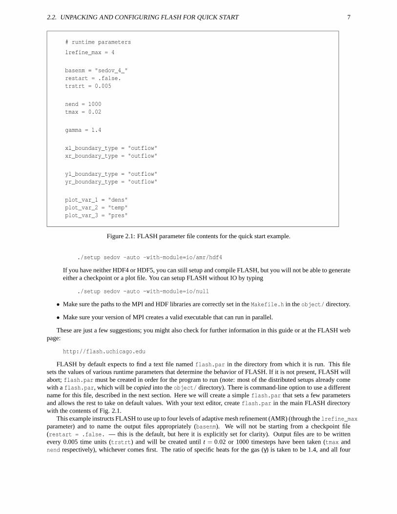
# runtime parameters
lrefine_max = 4
basenm = "sedov_4_"restart = .false.trstrt = 0.005
nend = 1000tmax = 0.02
gamma = 1.4
xl_boundary_type = "outflow"xr_boundary_type = "outflow"
yl_boundary_type = "outflow"yr_boundary_type = "outflow"
plot_var_1 = "dens"plot_var_2 = "temp"plot_var_3 = "pres"
Figure 2.1: FLASH parameter file contents for the quick start example.
./setup sedov -auto -with-module=io/amr/hdf4
If you have neither HDF4 or HDF5, you can still setup and compile FLASH, but you will not be able to generateeither a checkpoint or a plot file. You can setup FLASH without IO by typing
./setup sedov -auto -with-module=io/null
• Make sure the paths to the MPI and HDF libraries are correctly set in the Makefile.h in the object/ directory.
• Make sure your version of MPI creates a valid executable that can run in parallel.
These are just a few suggestions; you might also check for further information in this guide or at the FLASH webpage:
http://flash.uchicago.edu
FLASH by default expects to find a text file named flash.par in the directory from which it is run. This filesets the values of various runtime parameters that determine the behavior of FLASH. If it is not present, FLASH willabort; flash.par must be created in order for the program to run (note: most of the distributed setups already comewith a flash.par, which will be copied into the object/ directory). There is command-line option to use a differentname for this file, described in the next section. Here we will create a simple flash.par that sets a few parametersand allows the rest to take on default values. With your text editor, create flash.par in the main FLASH directorywith the contents of Fig. 2.1.
This example instructs FLASH to use up to four levels of adaptive mesh refinement (AMR) (through the lrefine_maxparameter) and to name the output files appropriately (basenm). We will not be starting from a checkpoint file(restart = .false. — this is the default, but here it is explicitly set for clarity). Output files are to be writtenevery 0.005 time units (trstrt) and will be created until t = 0.02 or 1000 timesteps have been taken (tmax andnend respectively), whichever comes first. The ratio of specific heats for the gas (γ) is taken to be 1.4, and all four
8 CHAPTER 2. QUICK START
boundaries of the two-dimensional grid have outflow (zero-gradient or Neumann) boundary conditions (see via the[xy][lr]_boundary_type parameters).
Note the format of the file – each line is a comment (denoted by a hash mark, #), blank, or of the form variable =value. String values are enclosed in double quotes ("). Boolean values are indicated in the Fortran style, .true. or.false. Be sure to insert a carriage return after the last line of text. A full list of the parameters available for yourcurrent setup is contained in paramFile.txt, which also includes brief comments for each parameter. If you wish toskip the creation of a flash.par, a complete example is provided in the setups/sedov/ directory.
2.3 Running FLASH
We are now ready to run FLASH. To run FLASH on N processors, type
mpirun -np N object/flashX
remembering to replace N and X with the appropriate values. Some systems may require you to start MPI programswith a different command; use whichever command is appropriate for your system. The FLASH executable can taketwo command-line arguments, the name of the runtime parameter file (-par_file <filename>), and the name ofcheckpoint file (-chk_file <filename>). If the -par_file is found, FLASH reads the file specified on command linefor runtime parameters, otherwise it reads flash.par. If the -chk_file is found, FLASH assumes that it is startingfrom restart, and it gets the runtime parameters from the file specified on the command line. In this situation flash.paris ignored. If both the arguments are present, the par_file argument is ignored and runtime parameters are read fromthe checkpoint file specified on command line.
You should see a number of lines of output indicating that FLASH is initializing the Sedov problem, listing theinitial parameters, and giving the timestep chosen at each step. After the run is finished, you should find several filesin the current directory:
• flash.log echoes the runtime parameter settings and indicates the run time, the build time, and the buildmachine. During the run, a line is written for each timestep, along with any warning messages. If the runterminates normally, a performance summary is written to this file. Messages indicating when the code refinedand what output resulted are also contained in flash.log.
• flash.dat contains a number of integral quantities as functions of time: total mass, total energy, total momen-tum, etc. This file can be used directly by plotting programs such as gnuplot; note that the first line begins witha hash (#) and is thus ignored by gnuplot.
• sedov_4_hdf5_chk_000* are the different checkpoint files. These are complete dumps of the entire simulationat intervals of trstrt and are suitable for use in restarting the simulation. They are also the primary outputproducts of FLASH.
• sedov_4_hdf5_plt_cnt_000* are plot files. These are files containing only density, temperature, and pressure(in single precision for some I/O modules). They are designed to be written more frequently than checkpointfiles for the purpose of making simulation movies (or for analyses that do not require all of the checkpointedquantities).
• amr_log includes various messages from the PARAMESH adaptive mesh refinement package.
We will use the xflash routine under IDL to examine the output. Before doing so, we need to set the values of twoenvironment variables, IDL_PATH and XFLASH_DIR. Under csh this can be done using the commands
setenv XFLASH_DIR "$PWD/tools/fidlr3"setenv IDL_PATH "$XFLASH_DIR:$IDL_PATH"
If you get a message indicating that IDL_PATH is not defined, enter
setenv IDL_PATH "$XFLASH_DIR":idl-root-path:idl-root-path/lib
2.3. RUNNING FLASH 9
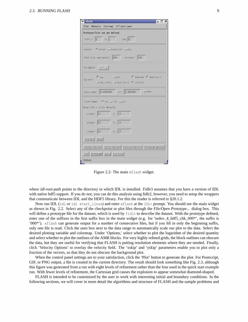
Figure 2.2: The main xflash widget.
where idl-root-path points to the directory in which IDL is installed. Fidlr3 assumes that you have a version of IDLwith native hdf5 support. If you do not, you can do this analysis using fidlr2, however, you need to setup the wrappersthat communicate between IDL and the HDF5 library. For this the reader is referred to §20.1.2.
Now run IDL (idl or idl start_linux) and enter xflash at the IDL> prompt. You should see the main widgetas shown in Fig. 2.2. Select any of the checkpoint or plot files through the File/Open Prototype... dialog box. Thiswill define a prototype file for the dataset, which is used by fidlr to describe the dataset. With the prototype defined,enter one of the suffixes in the first suffix box in the main widget (e.g. for ’sedov_4_hdf5_chk_000*’, the suffix is’000*’). xflash can generate output for a number of consecutive files, but if you fill in only the beginning suffix,only one file is read. Click the auto box next to the data range to automatically scale our plot to the data. Select thedesired plotting variable and colormap. Under ‘Options,’ select whether to plot the logarithm of the desired quantityand select whether to plot the outlines of the AMR blocks. For very highly refined grids, the block outlines can obscurethe data, but they are useful for verifying that FLASH is putting resolution elements where they are needed. Finally,click ‘Velocity Options’ to overlay the velocity field. The ‘xskip’ and ‘yskip’ parameters enable you to plot only afraction of the vectors, so that they do not obscure the background plot.
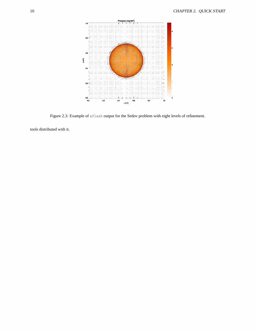
When the control panel settings are to your satisfaction, click the ‘Plot’ button to generate the plot. For Postscript,GIF, or PNG output, a file is created in the current directory. The result should look something like Fig. 2.3, althoughthis figure was generated from a run with eight levels of refinement rather than the four used in the quick start examplerun. With fewer levels of refinement, the Cartesian grid causes the explosion to appear somewhat diamond-shaped.
FLASH is intended to be customized by the user to work with interesting initial and boundary conditions. In thefollowing sections, we will cover in more detail the algorithms and structure of FLASH and the sample problems and
10 CHAPTER 2. QUICK START
Figure 2.3: Example of xflash output for the Sedov problem with eight levels of refinement.
tools distributed with it.
Chapter 3
The FLASH configuration script (setup)
The setup script, found in the FLASH root directory, provides the primary command-line interface to the FLASHsource code. It configures the source tree for a given problem and target machine and creates files needed to parsethe runtime parameter file and make the FLASH executable. More description of what setup does may be found inChapter 5. Here we describe its basic usage.
Running setup without any options prints a message describing the available options:
$ ./setupusage: setup <problem-name> [options]
problems: see setups/ directoryoptions: -auto -[123]d -maxblocks=<#> -nxb=<#> -nyb=<#> -nzb=<#>
-portable -verbose -force [-site=<site> | -ostype=<ostype>][-debug | -test] -preprocess -objdir=<relative obj directory>-with-module=<module> -io_convert=<from_iopath: to_iopath>
Available values for the mandatory option (the name of the problem to configure) are determined by scanning thesetups/ directory.
A “problem” consists of a set of initial and boundary conditions, possibly additional physics (e.g., a subgrid modelfor star formation), and a set of adjustable parameters. The directory associated with a problem contains sourcecode files that implement the initial conditions and, in a few cases, the boundary conditions and extra physics. Alsopresent is a configuration file, read by setup, which contains information on required physics modules and adjustableparameters.
setup determines site-dependent configuration information by looking in source/sites/ for a directory with thesame name as the output of the hostname command; failing this, it looks in the directory source/sites/Prototypes/for a directory with the same name as the output of the uname command. The site and operating system type can beoverridden with the -site and -ostype command-line options. Only one of these options can be used. The directoryfor each site or operating system type contains a makefile fragment (Makefile.h) that sets command names, compilerflags, library paths, and any replacement or additional source files needed to compile FLASH for that machine type.
setup uses the problem and site/OS type, together with a user-supplied file called Modules, which lists the codemodules to include, to generate a directory called object/ that contains links to the appropriate source files andmakefile fragments. It also creates the master makefile (object/Makefile) and several Fortran include files that areneeded by the code in order to parse the runtime parameter file. After running setup, the user can make the FLASHexecutable by running gmake in the object/ directory (or from the FLASH root directory, if the -portable optionis not used with setup). Parallel builds, using the -j argument to gmake should work and can significantly speed upthe build process.
The optional command-line modifiers have the following interpretations:
-verbose Normally setup echoes to the standard output summary messages indicating what it isdoing. Including the -verbose option causes it to also list the links it creates.
11
12 CHAPTER 3. THE FLASH CONFIGURATION SCRIPT (SETUP)
-portable This option creates a portable build directory by copying instead of linking to the sourcefiles in source/ and setups/. The resulting build directory can be placed into a tararchive and sent to another machine for building (use the Makefile created by setup in thetar file).
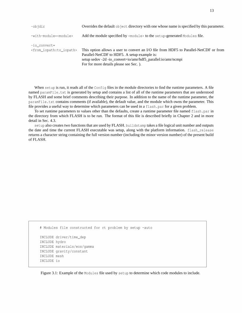
-auto This modifier replaces -defaults, which is still present in the code but has been depre-cated. Normally setup requires that the user supply a plain text file called Modules (in theFLASH root directory) that specifies which code modules to include. A sample Modulesfile appears in Fig. 3.1. Each line is either a comment (preceded by a hash mark (#)) ora module include statement of the form INCLUDE module. Sub-modules are indicated byspecifying the path to the sub-module in question; in the example, the sub-module gammaof the eos module is included. If a module has a default sub-module but no sub-module isspecified, setup automatically selects the default using the module’s configuration file.
The -auto option enables setup to generate a “rough draft” of a Modules file for theuser. The configuration file for each problem setup specifies a number of code mod-ule requirements; for example, a problem may require the perfect-gas equation of state(materials/eos/gamma) and an unspecified hydro solver (hydro). With -auto, setupcreates a Modules file by converting these requirements into module include statements.In addition, it checks the configuration files for the required modules and includes any oftheir required modules, eliminating duplicates. Most users configuring a problem for thefirst time will want to run setup with -auto to generate a Modules file and then will wantto edit Modules directly to specify different sub-modules. Alternatively, sub-modules canbe specified using the -with-module=<submodule path> along with -auto option, elim-inating the need to edit the Modules file. After editing Modules in this way, re-run setupwithout -auto to incorporate the changes into the code configuration.
-[123]d By default, setup creates a makefile which produces a FLASH executable capable of solv-ing two-dimensional problems (equivalent to -2d). To generate a makefile with optionsappropriate to three-dimensional problems, use -3d. To generate a one-dimensional code,use -1d. These options are mutually exclusive and cause setup to add the appropriatecompilation option to the makefile it generates.
-maxblocks=# This option is also used by setup in constructing the makefile compiler options. It deter-mines the amount of memory allocated at runtime to the adaptive mesh refinement (AMR)block data structure. For example, to allocate enough memory on each processor for 500blocks, use -maxblocks=500. If the default block buffer size is too large for your system,you may wish to try a smaller number here. Alternatively, you may wish to experimentwith larger buffer sizes, if your system has enough memory.
-nxb=# -nyb=# -nzb=# These options are also used by setup in constructing the makefile compiler options. Themesh on which the problem is solved is composed of blocks. These options determine thenumber of interior cells (not counting guard cells) for each block. The default value foreach of these options is 8.
-debug The default Makefile built by setup will use the optimized setting for compilation and link-ing. Using -debug will force setup to use the flags relevant for debugging (e.g., including-g in the compilation line).
-test When FLASH is tested by the automated test suite, testwill choose the proper compilationarguments for the test executable.
-preprocess This option will preprocess all of the files before compilation. This is useful for machineswhose compilers do not support preprocessing.
13
-objdir Overrides the default object directory with one whose name is specified by this parameter.
-with-module=<module> Add the module specified by <module> to the setup-generated Modules file.
-io_convert=<from_iopath:to_iopath> This option allows a user to convert an I/O file from HDF5 to Parallel-NetCDF or from
Parallel-NetCDF to HDF5. A setup example is:setup sedov -2d -io_convert=io/amr/hdf5_parallel:io/amr/ncmpiFor for more details please see Sec. ).
When setup is run, it reads all of the Config files in the module directories to find the runtime parameters. A filenamed paramFile.txt is generated by setup and contains a list of all of the runtime parameters that are understoodby FLASH and some brief comments describing their purpose. In addition to the name of the runtime parameter, theparamFile.txt contains comments (if available), the default value, and the module which owns the parameter. Thisfile provides a useful way to determine which parameters can be used in a flash.par for a given problem.
To set runtime parameters to values other than the defaults, create a runtime parameter file named flash.par inthe directory from which FLASH is to be run. The format of this file is described briefly in Chapter 2 and in moredetail in Sec. 4.3.
setup also creates two functions that are used by FLASH. buildstamp takes a file logical unit number and outputsthe date and time the current FLASH executable was setup, along with the platform information. flash_releasereturns a character string containing the full version number (including the minor version number) of the present buildof FLASH.
# Modules file constructed for rt problem by setup -auto
INCLUDE driver/time_depINCLUDE hydroINCLUDE materials/eos/gammaINCLUDE gravity/constantINCLUDE meshINCLUDE io
Figure 3.1: Example of the Modules file used by setup to determine which code modules to include.

14 CHAPTER 3. THE FLASH CONFIGURATION SCRIPT (SETUP)

Chapter 4
Setting up new problems
Every FLASH problem requires a directory in FLASH2.5/setups. This is where the FLASH setup script looksto find the problem-specific files. The FLASH distribution includes a number of pre-written setups. However, mostFLASH users will want to define their own problems, so it is important to understand the techniques for adding acustomized problem setup.
Each setups directory contains the routines that initialize the FLASH grid. The directory also includes parameterfiles that setup uses to select the proper physics modules from the FLASH source tree. When the user runs setup,the proper source files are selected and linked to the object/ directory (Chapter 3).
There are two files that must be included in the setup directory for any problem. These are
Config lists the modules required for the problem and defines additional runtimeparameters.
init_block.F90 Fortran routine for setting initial conditions in a single block.
We will look in detail at these files for an example setup. This is a simple setup which creates a domain with hotash inside a circle of radius radius centered at (xctr, yctr, zctr). The density is uniformly set at rho_ambient andthe temperature is t_perturb inside the circle and t_ambient outside.
To create a new setup, we first create the new directory and then add the Config and init_block.F90 files. Theeasiest way to construct these files is to use files from another setup as a template.
4.1 Creating a Config file
The simplest way to construct a Config file is to copy one from another setup that incorporates the same physicsas the new problem. Config serves two principal purposes: (1) to specify the required modules and (2) to registerruntime parameters. The Config file for the example problem contains the following:
# configuration file for our example problem
REQUIRES driver/time_depREQUIRES materials/eos/gammaREQUIRES materials/composition/fuel+ashREQUIRES ioREQUIRES meshREQUIRES hydro
These lines define the FLASH modules required by the setup. We are going to carry two fluids (fuel and ash), sowe require the composition module fuel+ash. At runtime, this module will initialize the multifluid database to carrythe two fluids and set up their properties. We also require I/O, meshing, and hydrodynamics, but we do not specifyparticular sub-modules of these modules; any sub-modules of io, mesh, and hydro will satisfy these requirements.
15
16 CHAPTER 4. SETTING UP NEW PROBLEMS
However, we require the simple gamma-law equation of state (materials/eos/gamma) for this problem, so we specifyit explicitly. In constructing the list of requirements for a problem, it is important to keep them as general as theproblem allows. Specific modules satisfying the requirements are given in the Modules file when we actually runsetup (the Modules file and its format are introduced in Chapter 3).
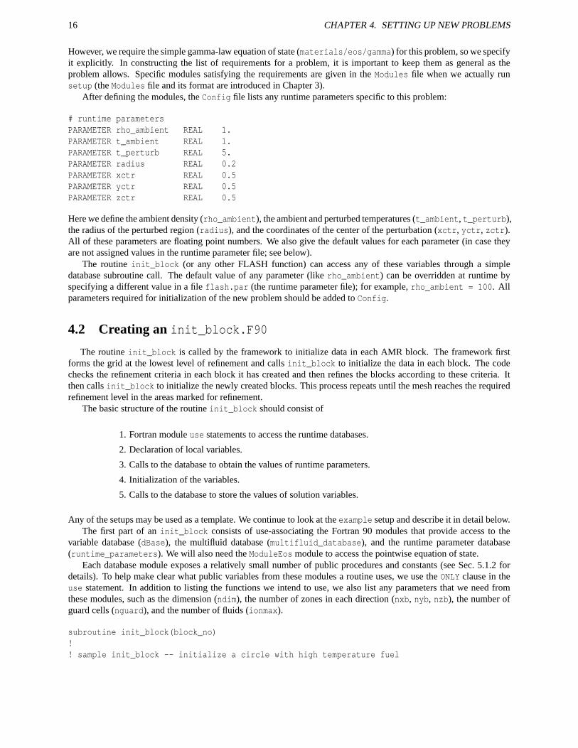
After defining the modules, the Config file lists any runtime parameters specific to this problem:
# runtime parametersPARAMETER rho_ambient REAL 1.PARAMETER t_ambient REAL 1.PARAMETER t_perturb REAL 5.PARAMETER radius REAL 0.2PARAMETER xctr REAL 0.5PARAMETER yctr REAL 0.5PARAMETER zctr REAL 0.5
Here we define the ambient density (rho_ambient), the ambient and perturbed temperatures (t_ambient, t_perturb),the radius of the perturbed region (radius), and the coordinates of the center of the perturbation (xctr, yctr, zctr).All of these parameters are floating point numbers. We also give the default values for each parameter (in case theyare not assigned values in the runtime parameter file; see below).
The routine init_block (or any other FLASH function) can access any of these variables through a simpledatabase subroutine call. The default value of any parameter (like rho_ambient) can be overridden at runtime byspecifying a different value in a file flash.par (the runtime parameter file); for example, rho_ambient = 100. Allparameters required for initialization of the new problem should be added to Config.
4.2 Creating an init_block.F90
The routine init_block is called by the framework to initialize data in each AMR block. The framework firstforms the grid at the lowest level of refinement and calls init_block to initialize the data in each block. The codechecks the refinement criteria in each block it has created and then refines the blocks according to these criteria. Itthen calls init_block to initialize the newly created blocks. This process repeats until the mesh reaches the requiredrefinement level in the areas marked for refinement.
The basic structure of the routine init_block should consist of
1. Fortran module use statements to access the runtime databases.
2. Declaration of local variables.
3. Calls to the database to obtain the values of runtime parameters.
4. Initialization of the variables.
5. Calls to the database to store the values of solution variables.
Any of the setups may be used as a template. We continue to look at the example setup and describe it in detail below.The first part of an init_block consists of use-associating the Fortran 90 modules that provide access to the
variable database (dBase), the multifluid database (multifluid_database), and the runtime parameter database(runtime_parameters). We will also need the ModuleEos module to access the pointwise equation of state.
Each database module exposes a relatively small number of public procedures and constants (see Sec. 5.1.2 fordetails). To help make clear what public variables from these modules a routine uses, we use the ONLY clause in theuse statement. In addition to listing the functions we intend to use, we also list any parameters that we need fromthese modules, such as the dimension (ndim), the number of zones in each direction (nxb, nyb, nzb), the number ofguard cells (nguard), and the number of fluids (ionmax).
subroutine init_block(block_no)!! sample init_block -- initialize a circle with high temperature fuel
4.2. CREATING AN INIT_BLOCK.F90 17
! surrounded by ash.!use multifluid_database, ONLY: find_fluid_index
use runtime_parameters, ONLY: get_parm_from_context, GLOBAL_PARM_CONTEXT
use dBase, ONLY: nxb, nyb, nzb, nguard, ionmax, &k2d, k3d, ndim, &CARTESIAN, &dBasePropertyInteger, &dBaseKeyNumber, dBaseSpecies, &dBaseGetCoords, dBasePutData
use ModuleEos, ONLY: eos
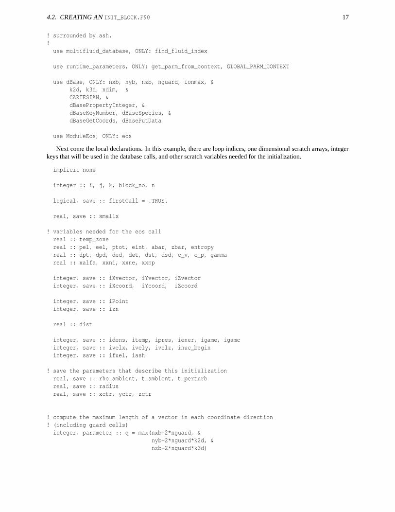
Next come the local declarations. In this example, there are loop indices, one dimensional scratch arrays, integerkeys that will be used in the database calls, and other scratch variables needed for the initialization.
implicit none
integer :: i, j, k, block_no, n
logical, save :: firstCall = .TRUE.
real, save :: smallx
! variables needed for the eos callreal :: temp_zonereal :: pel, eel, ptot, eint, abar, zbar, entropyreal :: dpt, dpd, ded, det, dst, dsd, c_v, c_p, gammareal :: xalfa, xxni, xxne, xxnp
integer, save :: iXvector, iYvector, iZvectorinteger, save :: iXcoord, iYcoord, iZcoord
integer, save :: iPointinteger, save :: izn
real :: dist
integer, save :: idens, itemp, ipres, iener, igame, igamcinteger, save :: ivelx, ively, ivelz, inuc_begininteger, save :: ifuel, iash
! save the parameters that describe this initializationreal, save :: rho_ambient, t_ambient, t_perturbreal, save :: radiusreal, save :: xctr, yctr, zctr
! compute the maximum length of a vector in each coordinate direction! (including guard cells)integer, parameter :: q = max(nxb+2*nguard, &
nyb+2*nguard*k2d, &nzb+2*nguard*k3d)
18 CHAPTER 4. SETTING UP NEW PROBLEMS
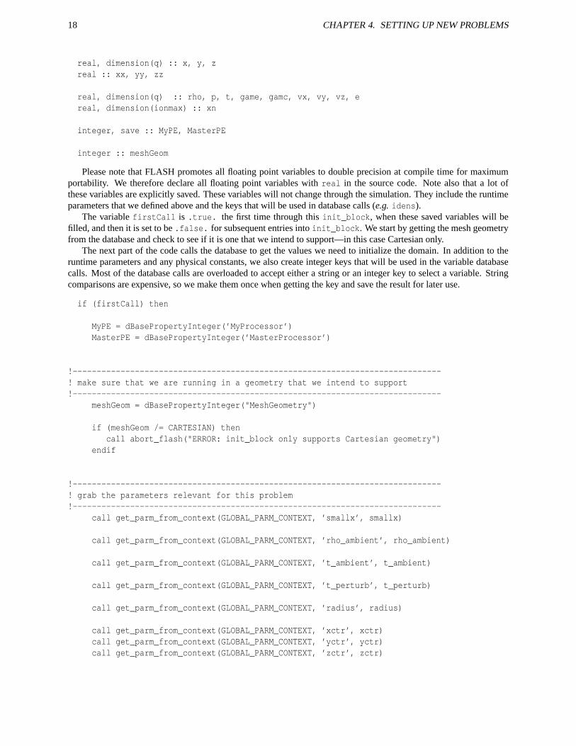
real, dimension(q) :: x, y, zreal :: xx, yy, zz
real, dimension(q) :: rho, p, t, game, gamc, vx, vy, vz, ereal, dimension(ionmax) :: xn
integer, save :: MyPE, MasterPE
integer :: meshGeom
Please note that FLASH promotes all floating point variables to double precision at compile time for maximumportability. We therefore declare all floating point variables with real in the source code. Note also that a lot ofthese variables are explicitly saved. These variables will not change through the simulation. They include the runtimeparameters that we defined above and the keys that will be used in database calls (e.g. idens).
The variable firstCall is .true. the first time through this init_block, when these saved variables will befilled, and then it is set to be .false. for subsequent entries into init_block. We start by getting the mesh geometryfrom the database and check to see if it is one that we intend to support—in this case Cartesian only.
The next part of the code calls the database to get the values we need to initialize the domain. In addition to theruntime parameters and any physical constants, we also create integer keys that will be used in the variable databasecalls. Most of the database calls are overloaded to accept either a string or an integer key to select a variable. Stringcomparisons are expensive, so we make them once when getting the key and save the result for later use.
if (firstCall) then
MyPE = dBasePropertyInteger(’MyProcessor’)MasterPE = dBasePropertyInteger(’MasterProcessor’)
!-----------------------------------------------------------------------------! make sure that we are running in a geometry that we intend to support!-----------------------------------------------------------------------------
meshGeom = dBasePropertyInteger("MeshGeometry")
if (meshGeom /= CARTESIAN) thencall abort_flash("ERROR: init_block only supports Cartesian geometry")
endif
!-----------------------------------------------------------------------------! grab the parameters relevant for this problem!-----------------------------------------------------------------------------
call get_parm_from_context(GLOBAL_PARM_CONTEXT, ’smallx’, smallx)
call get_parm_from_context(GLOBAL_PARM_CONTEXT, ’rho_ambient’, rho_ambient)
call get_parm_from_context(GLOBAL_PARM_CONTEXT, ’t_ambient’, t_ambient)
call get_parm_from_context(GLOBAL_PARM_CONTEXT, ’t_perturb’, t_perturb)
call get_parm_from_context(GLOBAL_PARM_CONTEXT, ’radius’, radius)
call get_parm_from_context(GLOBAL_PARM_CONTEXT, ’xctr’, xctr)call get_parm_from_context(GLOBAL_PARM_CONTEXT, ’yctr’, yctr)call get_parm_from_context(GLOBAL_PARM_CONTEXT, ’zctr’, zctr)
4.2. CREATING AN INIT_BLOCK.F90 19
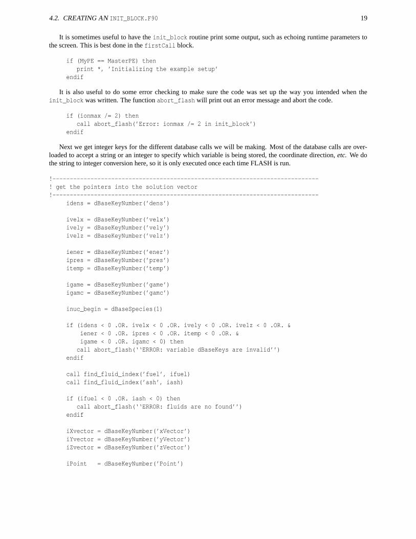
It is sometimes useful to have the init_block routine print some output, such as echoing runtime parameters tothe screen. This is best done in the firstCall block.
if (MyPE == MasterPE) thenprint *, ’Initializing the example setup’
endif
It is also useful to do some error checking to make sure the code was set up the way you intended when theinit_block was written. The function abort_flash will print out an error message and abort the code.
if (ionmax /= 2) thencall abort_flash(’Error: ionmax /= 2 in init_block’)
endif
Next we get integer keys for the different database calls we will be making. Most of the database calls are over-loaded to accept a string or an integer to specify which variable is being stored, the coordinate direction, etc. We dothe string to integer conversion here, so it is only executed once each time FLASH is run.
!-----------------------------------------------------------------------------! get the pointers into the solution vector!-----------------------------------------------------------------------------
idens = dBaseKeyNumber(’dens’)
ivelx = dBaseKeyNumber(’velx’)ively = dBaseKeyNumber(’vely’)ivelz = dBaseKeyNumber(’velz’)
iener = dBaseKeyNumber(’ener’)ipres = dBaseKeyNumber(’pres’)itemp = dBaseKeyNumber(’temp’)
igame = dBaseKeyNumber(’game’)igamc = dBaseKeyNumber(’gamc’)
inuc_begin = dBaseSpecies(1)
if (idens < 0 .OR. ivelx < 0 .OR. ively < 0 .OR. ivelz < 0 .OR. &iener < 0 .OR. ipres < 0 .OR. itemp < 0 .OR. &igame < 0 .OR. igamc < 0) then
call abort_flash(‘‘ERROR: variable dBaseKeys are invalid’’)endif
call find_fluid_index(’fuel’, ifuel)call find_fluid_index(’ash’, iash)
if (ifuel < 0 .OR. iash < 0) thencall abort_flash(‘‘ERROR: fluids are no found’’)
endif
iXvector = dBaseKeyNumber(’xVector’)iYvector = dBaseKeyNumber(’yVector’)iZvector = dBaseKeyNumber(’zVector’)
iPoint = dBaseKeyNumber(’Point’)
20 CHAPTER 4. SETTING UP NEW PROBLEMS
iXcoord = dBaseKeyNumber(’xCoord’)iYcoord = dBaseKeyNumber(’yCoord’)iZcoord = dBaseKeyNumber(’zCoord’)
izn = dBaseKeyNumber(’zn’)
if (iXvector < 0 .OR. iYvector < 0 .OR. iZvector < 0 .OR. iPoint < 0 .OR. &iXcoord < 0 .OR. iYcoord < 0 .OR. iZcoord < 0 .OR. izn < 0) then
call abort_flash(‘‘ERROR: coordinate dBaseKeys are invalid’’)endif
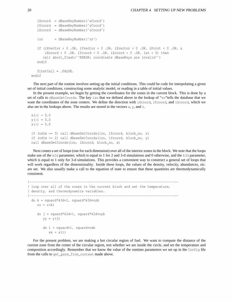
firstCall = .FALSE.endif
The next part of the routine involves setting up the initial conditions. This could be code for interpolating a givenset of initial conditions, constructing some analytic model, or reading in a table of initial values.
In the present example, we begin by getting the coordinates for the zones in the current block. This is done by aset of calls to dBaseGetCoords. The key izn that we defined above in the lookup of “zn”tells the database that wewant the coordinates of the zone centers. We define the direction with iXcoord, iYcoord, and iZcoord, which wealso set in the lookups above. The results are stored in the vectors x, y, and z.
x(:) = 0.0y(:) = 0.0z(:) = 0.0
if (ndim == 3) call dBaseGetCoords(izn, iZcoord, block_no, z)if (ndim >= 2) call dBaseGetCoords(izn, iYcoord, block_no, y)call dBaseGetCoords(izn, iXcoord, block_no, x)
Next comes a set of loops (one for each dimension) over all of the interior zones in the block. We note that the loopsmake use of the k2d parameter, which is equal to 1 for 2 and 3-d simulations and 0 otherwise, and the k3d parameter,which is equal to 1 only for 3-d simulations. This provides a convenient way to construct a general set of loops thatwill work regardless of the dimensionality. Inside these loops, the values of the density, velocity, abundances, etc.are set. We also usually make a call to the equation of state to ensure that these quantities are thermodynamicallyconsistent.
!-----------------------------------------------------------------------------! loop over all of the zones in the current block and set the temperature,! density, and thermodynamics variables.!-----------------------------------------------------------------------------do k = nguard*k3d+1, nguard*k3d+nzb
zz = z(k)
do j = nguard*k2d+1, nguard*k2d+nybyy = y(j)
do i = nguard+1, nguard+nxbxx = x(i)
For the present problem, we are making a hot circular region of fuel. We want to compute the distance of thecurrent zone from the center of the circular region, test whether we are inside the circle, and set the temperature andcomposition accordingly. Remember that we know the value of the runtime parameters we set up in the Config filefrom the calls to get_parm_from_context made above.
4.2. CREATING AN INIT_BLOCK.F90 21
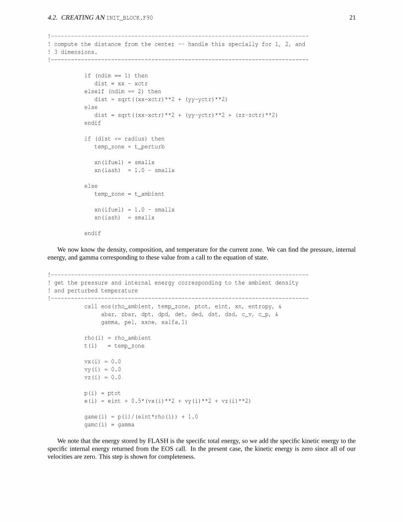
!-----------------------------------------------------------------------------! compute the distance from the center -- handle this specially for 1, 2, and! 3 dimensions.!-----------------------------------------------------------------------------
if (ndim == 1) thendist = xx - xctr
elseif (ndim == 2) thendist = sqrt((xx-xctr)**2 + (yy-yctr)**2)
elsedist = sqrt((xx-xctr)**2 + (yy-yctr)**2 + (zz-zctr)**2)
endif
if (dist <= radius) thentemp_zone = t_perturb
xn(ifuel) = smallxxn(iash) = 1.0 - smallx
elsetemp_zone = t_ambient
xn(ifuel) = 1.0 - smallxxn(iash) = smallx
endif
We now know the density, composition, and temperature for the current zone. We can find the pressure, internalenergy, and gamma corresponding to these value from a call to the equation of state.
!-----------------------------------------------------------------------------! get the pressure and internal energy corresponding to the ambient density! and perturbed temperature!-----------------------------------------------------------------------------
call eos(rho_ambient, temp_zone, ptot, eint, xn, entropy, &abar, zbar, dpt, dpd, det, ded, dst, dsd, c_v, c_p, &gamma, pel, xxne, xalfa,1)
rho(i) = rho_ambientt(i) = temp_zone
vx(i) = 0.0vy(i) = 0.0vz(i) = 0.0
p(i) = ptote(i) = eint + 0.5*(vx(i)**2 + vy(i)**2 + vz(i)**2)
game(i) = p(i)/(eint*rho(i)) + 1.0gamc(i) = gamma
We note that the energy stored by FLASH is the specific total energy, so we add the specific kinetic energy to thespecific internal energy returned from the EOS call. In the present case, the kinetic energy is zero since all of ourvelocities are zero. This step is shown for completeness.
22 CHAPTER 4. SETTING UP NEW PROBLEMS
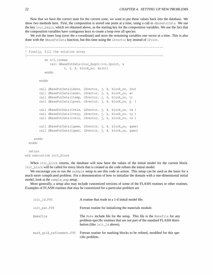
Now that we have the correct state for the current zone, we want to put these values back into the database. Weshow two methods here. First, the composition is stored one point at a time, using a call to dBasePutData. We usethe key inuc_begin, which we obtained above, as the starting key for the composition variables. We use the fact thatthe composition variables have contiguous keys to create a loop over all species.
We exit the inner loop (over the x-coordinate) and store the remaining variables one vector at a time. This is alsodone with the dBasePutData function, but this time using the iXvector key instead of iPoint.
!-----------------------------------------------------------------------------! finally, fill the solution array!-----------------------------------------------------------------------------
do n=1,ionmaxcall dBasePutData(inuc_begin-1+n,ipoint, &
i, j, k, block_no, xn(n))enddo
enddo
call dBasePutData(idens, iXvector, j, k, block_no, rho)call dBasePutData(iener, iXvector, j, k, block_no, e)call dBasePutData(itemp, iXvector, j, k, block_no, t)call dBasePutData(ipres, iXvector, j, k, block_no, p )
call dBasePutData(ivelx, iXvector, j, k, block_no, vx )call dBasePutData(ively, iXvector, j, k, block_no, vy )call dBasePutData(ivelz, iXvector, j, k, block_no, vz )
call dBasePutData(igame, iXvector, j, k, block_no, game)call dBasePutData(igamc, iXvector, j, k, block_no, gamc)
enddoenddo
returnend subroutine init_block
When init_block returns, the database will now have the values of the initial model for the current block.init_block will be called for every block that is created as the code refines the initial model.
We encourage you to run the example setup to see this code in action. This setup can be used as the basis for amuch more complicated problem. For a demonstration of how to initialize the domain with a one-dimensional initialmodel, look at the sample_map setup.
More generally, a setup also may include customized versions of some of the FLASH routines or other routines.Examples of FLASH routines that may be customized for a particular problem are
init_1d.F90 A routine that reads in a 1-d initial model file.
init_mat.F90 Fortran routine for initializing the materials module.
Makefile The Make include file for the setup. This file is the Makefile for anyproblem-specific routines that are not part of the standard FLASH distri-bution (like init_1d above).
mark_grid_refinement.F90 Fortran routine for marking blocks to be refined, modified for this spe-cific problem.
4.3. THE RUNTIME PARAMETER FILE (FLASH.PAR) 23
Users are encouraged to put any modifications of core FLASH files in the setups directory in which they are working.This makes it easier to distribute patches to our user base.
An additional file required to run the code is flash.par. It contains flags and parameters for running the code.Copies of flash.par may be kept in the setup directory for easy distribution.
4.3 The runtime parameter file (flash.par)
The file flash.par is read at runtime and sets the values of runtime parameters. The flash.par file for theexample setup is
# Parameters for the example setuprho_ambient = 1.0t_ambient = 1.0t_perturb = 10.radius = .2
# for starting a new runrestart = .false.cpnumber = 0ptnumber = 0
# dump checkpoint files every trstrt secondstrstrt = 4.0e-4
# dump plot files every tplot secondstplot = 5.0e-5
# go for nend steps or tmax seconds, whichever comes firstnend = 1000tmax = 1.0e5
# initial, and minimum timestepsdtini = 1.0e-16dtmin = 1.0e-20dtmax = 1.0e2
# Grid geometrygeometry = "cartesian"
# Size of computational volumexmin = 0.0xmax = 1.0ymin = 0.0ymax = 1.0zmin = 0.0zmax = 1.0
# Boundary conditionsxl_boundary_type = "outflow"xr_boundary_type = "outflow"yl_boundary_type = "outflow"yr_boundary_type = "outflow"zl_boundary_type = "outflow"zr_boundary_type = "outflow"
24 CHAPTER 4. SETTING UP NEW PROBLEMS
# Variables for refinement testrefine_var_1 = "dens"refine_var_2 = "pres"refine_var_3 = "none"refine_var_4 = "none"
# Refinement levelslrefine_max = 3lrefine_min = 1
# Number of lowest-level blocksnblockx = 1nblocky = 1nblockz = 1
# Hydrodynamics parameterscfl = 0.8
# Simulation-specific parametersbasenm = "example_3lev_"run_number = "001"run_comment = "A simple FLASH 2.5 example"log_file = "flash_example.log"
In this example, flags are set for a “cold start” of the simulation, grid geometry, boundary conditions, and refine-ment. Parameters are also set for the ambient temperature and density and for details of the run, such as the numberof timesteps between checkpoint files, and the initial, minimum and final values of the timestep.
setup produces a file named paramFile.txt each time it is run. This file lists all possible runtime parametersand the values to which they were set initially, as well as a brief description of the parameters.
Running the example setup with the -auto option and the flash.par provided will produce five checkpoint filesand 29 plot files. The initial temperature distribution, as visualized by the magic of the fidlr tools, appears in Fig. 4.1
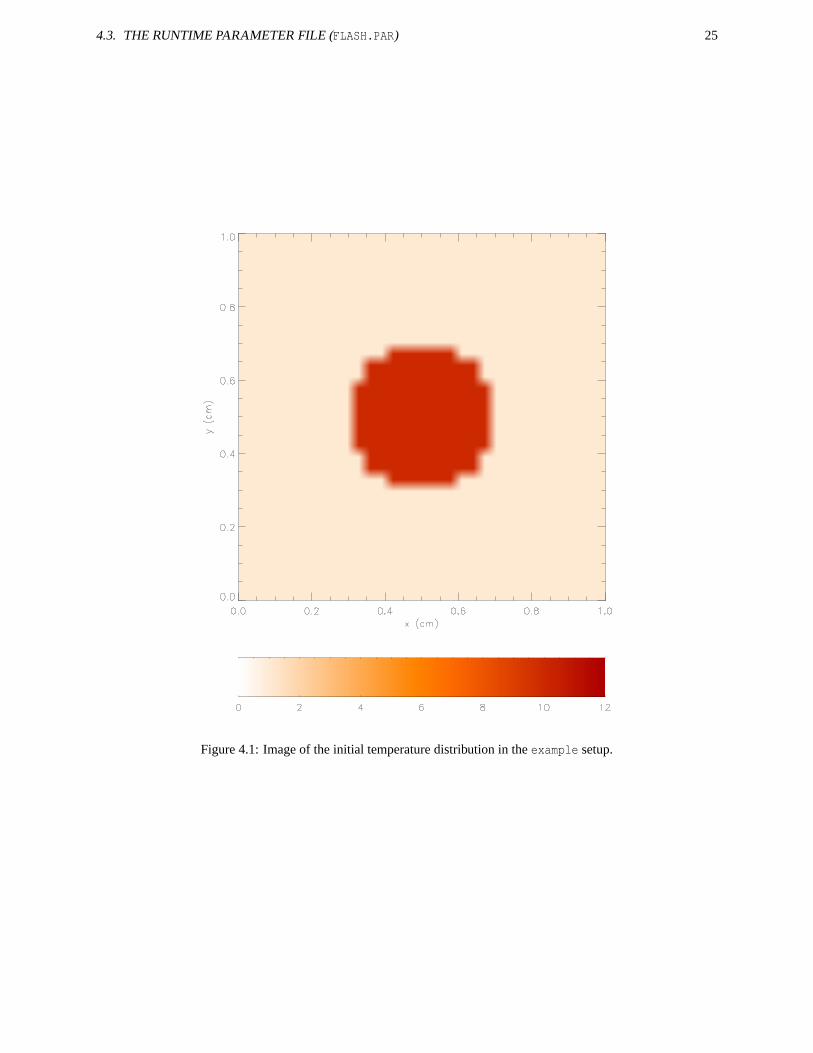
4.3. THE RUNTIME PARAMETER FILE (FLASH.PAR) 25
Figure 4.1: Image of the initial temperature distribution in the example setup.

26 CHAPTER 4. SETTING UP NEW PROBLEMS
Part II
Structure and Modules
27


Chapter 5
Overview of FLASH architecture
The FLASH source code is a collection of components called FLASH modules. FLASH modules can be combinedin a variety of ways to form specific FLASH applications. Of course, not all available FLASH modules are necessarilyused when solving any one particular problem. Thus, it is important to distinguish between the entire FLASH sourcecode and a given FLASH application.
5.1 Structure of a FLASH module
Most generally, a FLASH module represents some well-defined, top-level unit of functionality useful for a givenclass of problems. Its structure conforms to a small set of rules that facilitate its interactions with other modules in thecreation of an application. Primary among these are the rules governing the retrieval and modification of data on thesolution grid. A module must also announce a general set of requirements to the framework as well as publish a publicinterface of its services. Here we focus on the internal structure of a FLASH module appropriate for users wishing toextend the current FLASH functionality.
First, it is important to recall how a selected group of FLASH modules is combined to form a particular application.This process is carried out entirely by the FLASH setup tool, which uses configuration information provided by themodules and problem setup to properly parse the source tree and isolate the source files needed to set-up a specificproblem. For performance reasons, setup ties modules together statically before the application is compiled.
Each FLASH module is divided into three principal components:
a) Configuration layerb) “Wrapper” or “interface” layerc) Algorithm
Additionally, a module may contain sub-modules which inherit from and override the functionality in the parentmodule. Each of these components is discussed in detail in the following sections.
5.1.1 Configuration layer
Information about module dependencies, default sub-modules, runtime parameter definitions, library requirements,and so on is stored in plain text files named Config in the different module directories. These are parsed by setupwhen configuring the source tree and are used to create the code needed to register module variables, to implementthe runtime parameters, to choose sub-modules when only a generic module has been specified, to prevent mutuallyexclusive modules from being included together, and to flag problems when dependencies are not resolved by someincluded module. In the future they may contain additional information about module interrelationships.
5.1.1.1 Configuration file syntax
The syntax of the configuration files is as follows. Arbitrarily many spaces and/or tabs may be used, but all keywordsmust be in uppercase. Lines not matching an admissible pattern will raise an error when running setup.
29
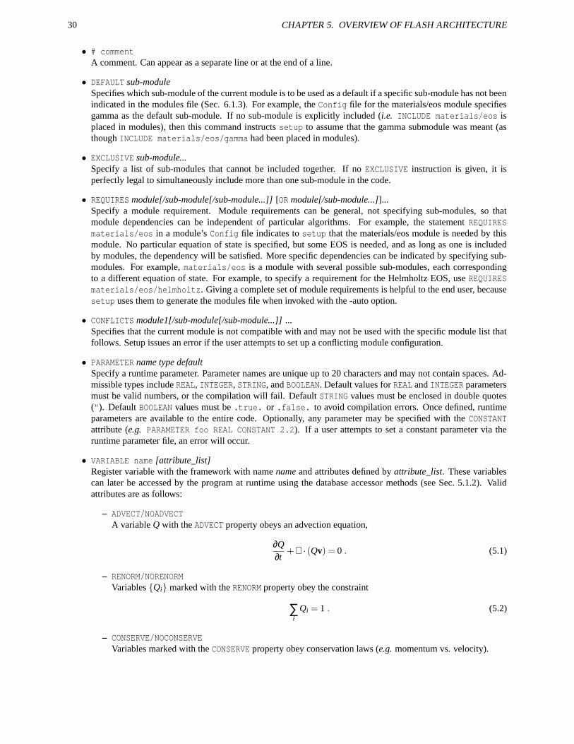
30 CHAPTER 5. OVERVIEW OF FLASH ARCHITECTURE
• # commentA comment. Can appear as a separate line or at the end of a line.
• DEFAULT sub-moduleSpecifies which sub-module of the current module is to be used as a default if a specific sub-module has not beenindicated in the modules file (Sec. 6.1.3). For example, the Config file for the materials/eos module specifiesgamma as the default sub-module. If no sub-module is explicitly included (i.e. INCLUDE materials/eos isplaced in modules), then this command instructs setup to assume that the gamma submodule was meant (asthough INCLUDE materials/eos/gamma had been placed in modules).
• EXCLUSIVE sub-module...Specify a list of sub-modules that cannot be included together. If no EXCLUSIVE instruction is given, it isperfectly legal to simultaneously include more than one sub-module in the code.
• REQUIRES module[/sub-module[/sub-module...]] [OR module[/sub-module...]]...Specify a module requirement. Module requirements can be general, not specifying sub-modules, so thatmodule dependencies can be independent of particular algorithms. For example, the statement REQUIRESmaterials/eos in a module’s Config file indicates to setup that the materials/eos module is needed by thismodule. No particular equation of state is specified, but some EOS is needed, and as long as one is includedby modules, the dependency will be satisfied. More specific dependencies can be indicated by specifying sub-modules. For example, materials/eos is a module with several possible sub-modules, each correspondingto a different equation of state. For example, to specify a requirement for the Helmholtz EOS, use REQUIRESmaterials/eos/helmholtz. Giving a complete set of module requirements is helpful to the end user, becausesetup uses them to generate the modules file when invoked with the -auto option.
• CONFLICTS module1[/sub-module[/sub-module...]] ...Specifies that the current module is not compatible with and may not be used with the specific module list thatfollows. Setup issues an error if the user attempts to set up a conflicting module configuration.
• PARAMETER name type defaultSpecify a runtime parameter. Parameter names are unique up to 20 characters and may not contain spaces. Ad-missible types include REAL, INTEGER, STRING, and BOOLEAN. Default values for REAL and INTEGER parametersmust be valid numbers, or the compilation will fail. Default STRING values must be enclosed in double quotes("). Default BOOLEAN values must be .true. or .false. to avoid compilation errors. Once defined, runtimeparameters are available to the entire code. Optionally, any parameter may be specified with the CONSTANTattribute (e.g. PARAMETER foo REAL CONSTANT 2.2). If a user attempts to set a constant parameter via theruntime parameter file, an error will occur.
• VARIABLE name [attribute_list]Register variable with the framework with name name and attributes defined by attribute_list. These variablescan later be accessed by the program at runtime using the database accessor methods (see Sec. 5.1.2). Validattributes are as follows:
– ADVECT/NOADVECTA variable Q with the ADVECT property obeys an advection equation,
∂Q∂t
+∇ · (Qv) = 0 . (5.1)
– RENORM/NORENORMVariables Qi marked with the RENORM property obey the constraint
∑i
Qi = 1 . (5.2)
– CONSERVE/NOCONSERVEVariables marked with the CONSERVE property obey conservation laws (e.g. momentum vs. velocity).
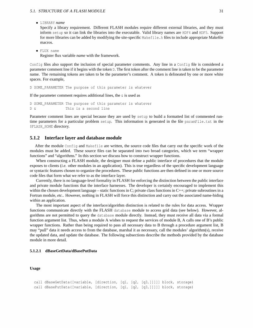
5.1. STRUCTURE OF A FLASH MODULE 31
• LIBRARY nameSpecify a library requirement. Different FLASH modules require different external libraries, and they mustinform setup so it can link the libraries into the executable. Valid library names are HDF4 and HDF5. Supportfor more libraries can be added by modifying the site-specific Makefile.h files to include appropriate Makefilemacros.
• FLUX nameRegister flux variable name with the framework.
Config files also support the inclusion of special parameter comments. Any line in a Config file is considered aparameter comment line if it begins with the token D. The first token after the comment line is taken to be the parametername. The remaining tokens are taken to be the parameter’s comment. A token is delineated by one or more whitespaces. For example,
D SOME_PARAMETER The purpose of this parameter is whatever
If the parameter comment requires additional lines, the & is used as
D SOME_PARAMETER The purpose of this parameter is whateverD & This is a second line
Parameter comment lines are special because they are used by setup to build a formatted list of commented run-time parameters for a particular problem setup. This information is generated in the file paramFile.txt in the$FLASH_HOME directory.
5.1.2 Interface layer and database module
After the module Config and Makefile are written, the source code files that carry out the specific work of themodules must be added. These source files can be separated into two broad categories, which we term “wrapperfunctions” and “algorithms.” In this section we discuss how to construct wrapper functions.
When constructing a FLASH module, the designer must define a public interface of procedures that the moduleexposes to clients (i.e. other modules in an application). This is true regardless of the specific development languageor syntactic features chosen to organize the procedures. These public functions are then defined in one or more sourcecode files that form what we refer to as the interface layer.
Currently, there is no language-level formality in FLASH for enforcing the distinction between the public interfaceand private module functions that the interface harnesses. The developer is certainly encouraged to implement thiswithin the chosen development language – static functions in C; private class functions in C++; private subroutines in aFortran module, etc.. However, nothing in FLASH will force this distinction and carry out the associated name-hidingwithin an application.
The most important aspect of the interface/algorithm distinction is related to the rules for data access. Wrapperfunctions communicate directly with the FLASH database module to access grid data (see below). However, al-gorithms are not permitted to query the database module directly. Instead, they must receive all data via a formalfunction argument list. Thus, when a module A wishes to request the services of module B, A calls one of B’s publicwrapper functions. Rather than being required to pass all necessary data to B through a procedure argument list, Bmay “pull” data it needs access to from the database, marshal it as necessary, call the modules’ algorithm(s), receivethe updated data, and update the database. The following subsections describe the methods provided by the databasemodule in more detail.
5.1.2.1 dBaseGetData/dBasePutData
Usage
call dBaseGetData([variable, [direction, [q1, [q2, [q3,]]]]] block, storage)call dBasePutData([variable, [direction, [q1, [q2, [q3,]]]]] block, storage)
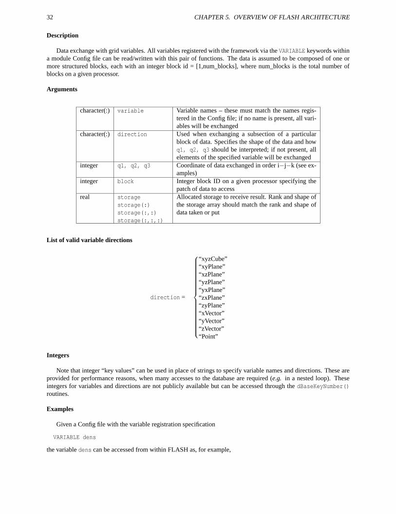
32 CHAPTER 5. OVERVIEW OF FLASH ARCHITECTURE
Description
Data exchange with grid variables. All variables registered with the framework via the VARIABLE keywords withina module Config file can be read/written with this pair of functions. The data is assumed to be composed of one ormore structured blocks, each with an integer block id = [1,num_blocks], where num_blocks is the total number ofblocks on a given processor.
Arguments
character(:) variable Variable names – these must match the names regis-tered in the Config file; if no name is present, all vari-ables will be exchanged
character(:) direction Used when exchanging a subsection of a particularblock of data. Specifies the shape of the data and howq1, q2, q3 should be interpreted; if not present, allelements of the specified variable will be exchanged
integer q1, q2, q3 Coordinate of data exchanged in order i−j−k (see ex-amples)
integer block Integer block ID on a given processor specifying thepatch of data to access
real storagestorage(:)storage(:,:)storage(:,:,:)
Allocated storage to receive result. Rank and shape ofthe storage array should match the rank and shape ofdata taken or put
List of valid variable directions
direction =
“xyzCube”“xyPlane”“xzPlane”“yzPlane”“yxPlane”“zxPlane”“zyPlane”“xVector”“yVector”“zVector”“Point”
Integers
Note that integer “key values” can be used in place of strings to specify variable names and directions. These areprovided for performance reasons, when many accesses to the database are required (e.g. in a nested loop). Theseintegers for variables and directions are not publicly available but can be accessed through the dBaseKeyNumber()routines.
Examples
Given a Config file with the variable registration specification
VARIABLE dens
the variable dens can be accessed from within FLASH as, for example,
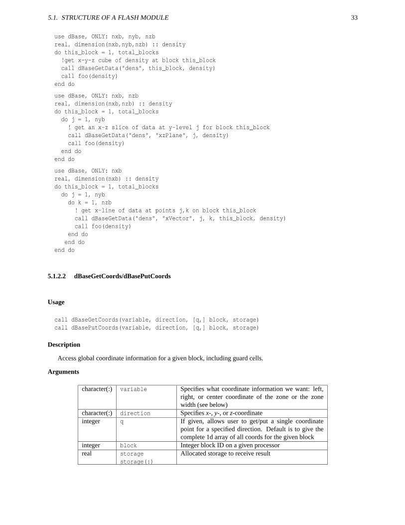
5.1. STRUCTURE OF A FLASH MODULE 33
use dBase, ONLY: nxb, nyb, nzbreal, dimension(nxb,nyb,nzb) :: densitydo this_block = 1, total_blocks!get x-y-z cube of density at block this_blockcall dBaseGetData("dens", this_block, density)call foo(density)
end do
use dBase, ONLY: nxb, nzbreal, dimension(nxb,nzb) :: densitydo this_block = 1, total_blocksdo j = 1, nyb! get an x-z slice of data at y-level j for block this_blockcall dBaseGetData("dens", "xzPlane", j, density)call foo(density)
end doend do
use dBase, ONLY: nxbreal, dimension(nxb) :: densitydo this_block = 1, total_blocksdo j = 1, nybdo k = 1, nzb! get x-line of data at points j,k on block this_blockcall dBaseGetData("dens", "xVector", j, k, this_block, density)call foo(density)
end doend do
end do
5.1.2.2 dBaseGetCoords/dBasePutCoords
Usage
call dBaseGetCoords(variable, direction, [q,] block, storage)call dBasePutCoords(variable, direction, [q,] block, storage)
Description
Access global coordinate information for a given block, including guard cells.
Arguments
character(:) variable Specifies what coordinate information we want: left,right, or center coordinate of the zone or the zonewidth (see below)
character(:) direction Specifies x-, y-, or z-coordinateinteger q If given, allows user to get/put a single coordinate
point for a specified direction. Default is to give thecomplete 1d array of all coords for the given block
integer block Integer block ID on a given processorreal storage
storage(:)Allocated storage to receive result
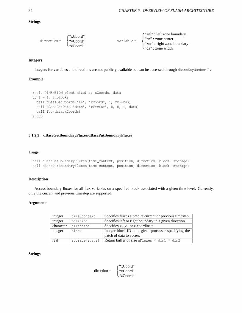
34 CHAPTER 5. OVERVIEW OF FLASH ARCHITECTURE
Strings
direction =
“xCoord”“yCoord”“zCoord”
variable =
“znl” : left zone boundary“zn” : zone center“znr” : right zone boundary“dz” : zone width
Integers
Integers for variables and directions are not publicly available but can be accessed through dBaseKeyNumber().
Example
real, DIMENSION(block_size) :: xCoords, datado i = 1, lnblockscall dBaseGetCoords("zn", "xCoord", i, xCoords)call dBaseGetData("dens", "xVector", 0, 0, i, data)call foo(data,xCoords)
enddo
5.1.2.3 dBaseGetBoundaryFluxes/dBasePutBoundaryFluxes
Usage
call dBaseGetBoundaryFluxes(time_context, position, direction, block, storage)call dBasePutBoundaryFluxes(time_context, position, direction, block, storage)
Description
Access boundary fluxes for all flux variables on a specified block associated with a given time level. Currently,only the current and previous timestep are supported.
Arguments
integer time_context Specifies fluxes stored at current or previous timestepinteger position Specifies left or right boundary in a given directioncharacter direction Specifies x-, y-, or z-coordinateinteger block Integer block ID on a given processor specifying the
patch of data to accessreal storage(:,:,:) Return buffer of size nFluxes * dim1 * dim2
Strings
direction =
“xCoord”“yCoord”“zCoord”
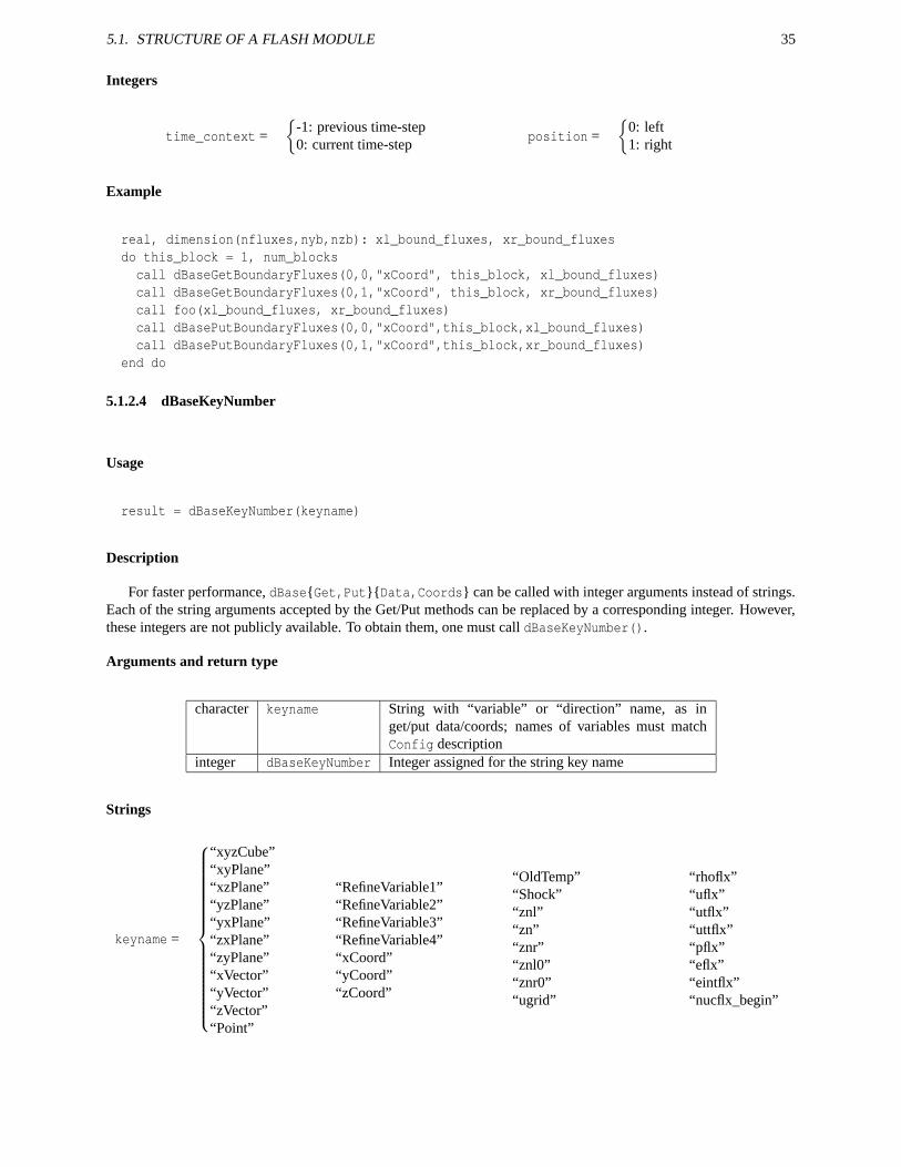
5.1. STRUCTURE OF A FLASH MODULE 35
Integers
time_context =
-1: previous time-step0: current time-step
position =
0: left1: right
Example
real, dimension(nfluxes,nyb,nzb): xl_bound_fluxes, xr_bound_fluxesdo this_block = 1, num_blockscall dBaseGetBoundaryFluxes(0,0,"xCoord", this_block, xl_bound_fluxes)call dBaseGetBoundaryFluxes(0,1,"xCoord", this_block, xr_bound_fluxes)call foo(xl_bound_fluxes, xr_bound_fluxes)call dBasePutBoundaryFluxes(0,0,"xCoord",this_block,xl_bound_fluxes)call dBasePutBoundaryFluxes(0,1,"xCoord",this_block,xr_bound_fluxes)
end do
5.1.2.4 dBaseKeyNumber
Usage
result = dBaseKeyNumber(keyname)
Description
For faster performance, dBaseGet,PutData,Coords can be called with integer arguments instead of strings.Each of the string arguments accepted by the Get/Put methods can be replaced by a corresponding integer. However,these integers are not publicly available. To obtain them, one must call dBaseKeyNumber().
Arguments and return type
character keyname String with “variable” or “direction” name, as inget/put data/coords; names of variables must matchConfig description
integer dBaseKeyNumber Integer assigned for the string key name
Strings
keyname =
“xyzCube”“xyPlane”“xzPlane”“yzPlane”“yxPlane”“zxPlane”“zyPlane”“xVector”“yVector”“zVector”“Point”
“RefineVariable1”“RefineVariable2”“RefineVariable3”“RefineVariable4”“xCoord”“yCoord”“zCoord”
“OldTemp”“Shock”“znl”“zn”“znr”“znl0”“znr0”“ugrid”
“rhoflx”“uflx”“utflx”“uttflx”“pflx”“eflx”“eintflx”“nucflx_begin”
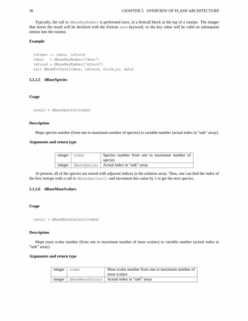
36 CHAPTER 5. OVERVIEW OF FLASH ARCHITECTURE
Typically, the call to dBaseKeyNumber is performed once, in a firstcall block at the top of a routine. The integerthat stores the result will be declared with the Fortran save keyword, so the key value will be valid on subsequententries into the routine.
Example
integer :: idens, ixCoordidens = dBaseKeyNumber("dens")ixCoord = dBaseKeyNumber("xCoord")call dBasePutData(idens, ixCoord, block_no, data)
5.1.2.5 dBaseSpecies
Usage
result = dBaseSpecies(index)
Description
Maps species number (from one to maximum number of species) to variable number (actual index in “unk” array).
Arguments and return type
integer index Species number from one to maximum number ofspecies
integer dBaseSpecies Actual index in “unk” array
At present, all of the species are stored with adjacent indices in the solution array. Thus, one can find the index ofthe first isotope with a call to dBaseSpecies(1) and increment this value by 1 to get the next species.
5.1.2.6 dBaseMassScalars
Usage
result = dBaseMassScalars(index)
Description
Maps mass scalar number (from one to maximum number of mass scalars) to variable number (actual index in“unk” array).
Arguments and return type
integer index Mass scalar number from one to maximum number ofmass scalars
integer dBaseMassScalars Actual index in “unk” array
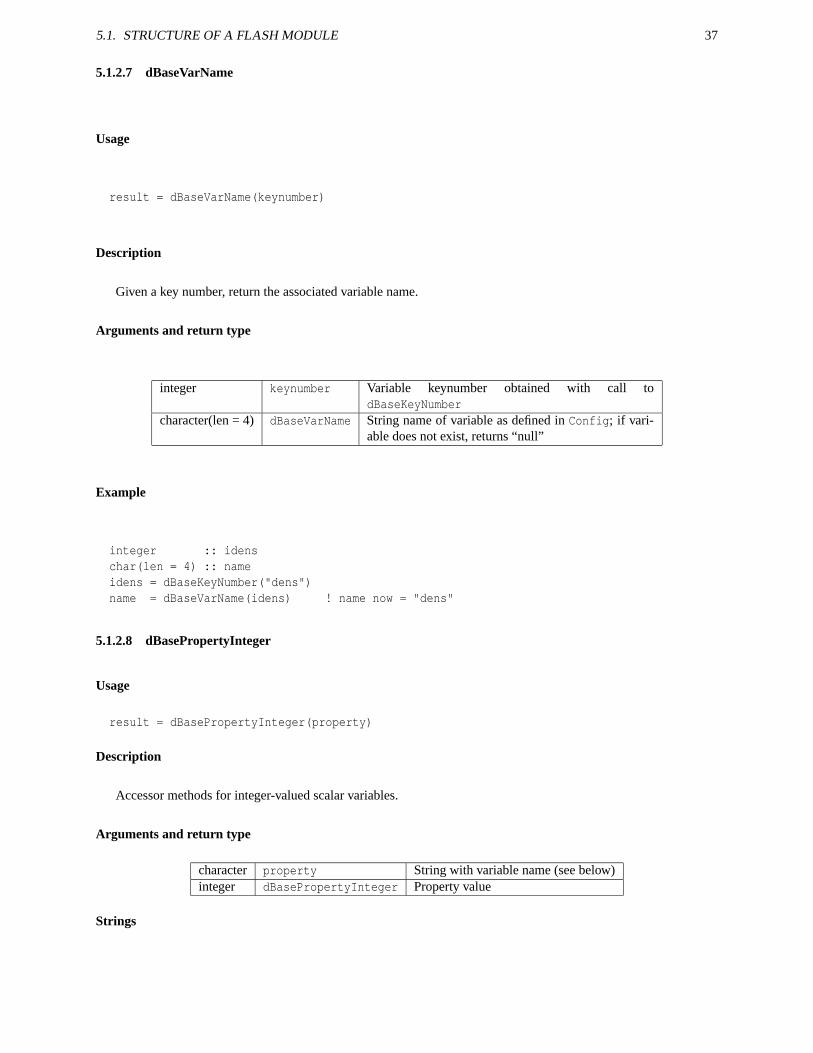
5.1. STRUCTURE OF A FLASH MODULE 37
5.1.2.7 dBaseVarName
Usage
result = dBaseVarName(keynumber)
Description
Given a key number, return the associated variable name.
Arguments and return type
integer keynumber Variable keynumber obtained with call todBaseKeyNumber
character(len = 4) dBaseVarName String name of variable as defined in Config; if vari-able does not exist, returns “null”
Example
integer :: idenschar(len = 4) :: nameidens = dBaseKeyNumber("dens")name = dBaseVarName(idens) ! name now = "dens"
5.1.2.8 dBasePropertyInteger
Usage
result = dBasePropertyInteger(property)
Description
Accessor methods for integer-valued scalar variables.
Arguments and return type
character property String with variable name (see below)integer dBasePropertyInteger Property value
Strings
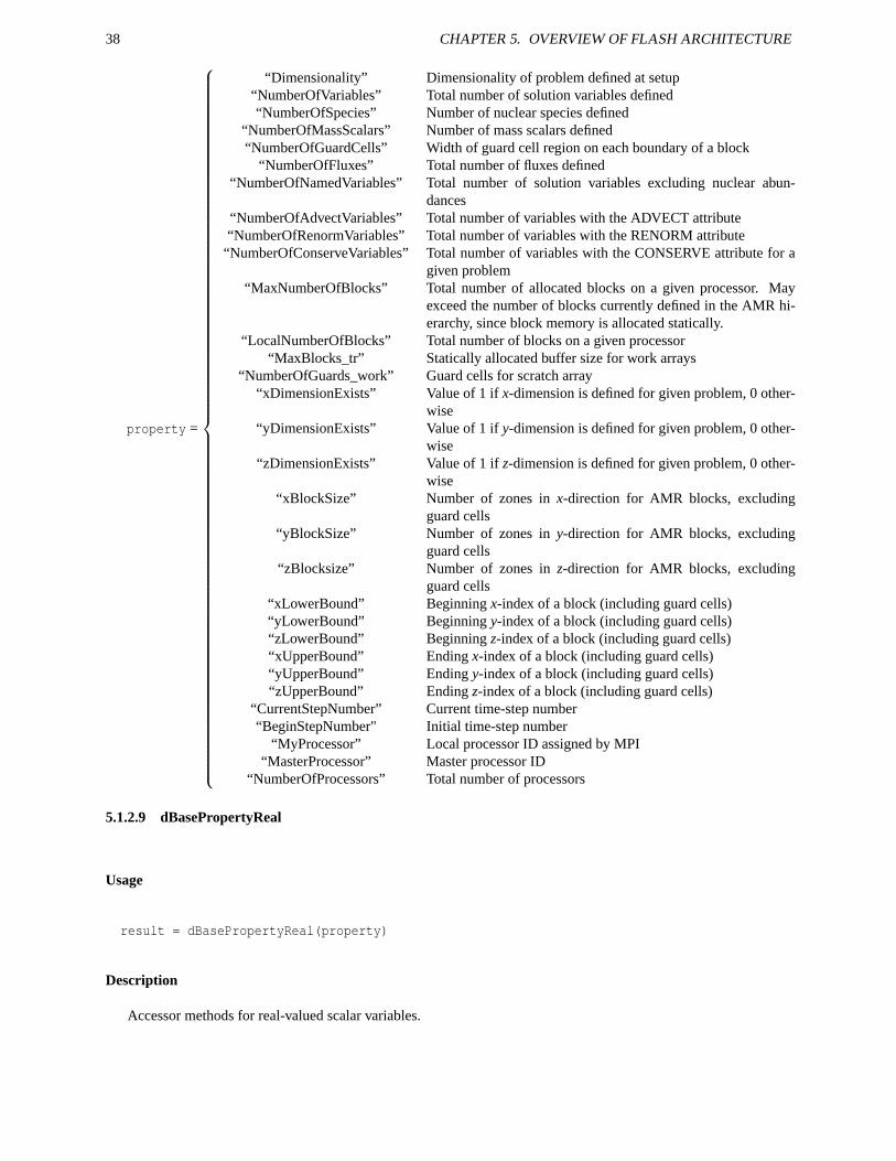
38 CHAPTER 5. OVERVIEW OF FLASH ARCHITECTURE
property =
“Dimensionality” Dimensionality of problem defined at setup“NumberOfVariables” Total number of solution variables defined“NumberOfSpecies” Number of nuclear species defined
“NumberOfMassScalars” Number of mass scalars defined“NumberOfGuardCells” Width of guard cell region on each boundary of a block
“NumberOfFluxes” Total number of fluxes defined“NumberOfNamedVariables” Total number of solution variables excluding nuclear abun-
dances“NumberOfAdvectVariables” Total number of variables with the ADVECT attribute“NumberOfRenormVariables” Total number of variables with the RENORM attribute
“NumberOfConserveVariables” Total number of variables with the CONSERVE attribute for agiven problem
“MaxNumberOfBlocks” Total number of allocated blocks on a given processor. Mayexceed the number of blocks currently defined in the AMR hi-erarchy, since block memory is allocated statically.
“LocalNumberOfBlocks” Total number of blocks on a given processor“MaxBlocks_tr” Statically allocated buffer size for work arrays
“NumberOfGuards_work” Guard cells for scratch array“xDimensionExists” Value of 1 if x-dimension is defined for given problem, 0 other-
wise“yDimensionExists” Value of 1 if y-dimension is defined for given problem, 0 other-
wise“zDimensionExists” Value of 1 if z-dimension is defined for given problem, 0 other-
wise“xBlockSize” Number of zones in x-direction for AMR blocks, excluding
guard cells“yBlockSize” Number of zones in y-direction for AMR blocks, excluding
guard cells“zBlocksize” Number of zones in z-direction for AMR blocks, excluding
guard cells“xLowerBound” Beginning x-index of a block (including guard cells)“yLowerBound” Beginning y-index of a block (including guard cells)“zLowerBound” Beginning z-index of a block (including guard cells)“xUpperBound” Ending x-index of a block (including guard cells)“yUpperBound” Ending y-index of a block (including guard cells)“zUpperBound” Ending z-index of a block (including guard cells)
“CurrentStepNumber” Current time-step number“BeginStepNumber" Initial time-step number
“MyProcessor” Local processor ID assigned by MPI“MasterProcessor” Master processor ID
“NumberOfProcessors” Total number of processors
5.1.2.9 dBasePropertyReal
Usage
result = dBasePropertyReal(property)
Description
Accessor methods for real-valued scalar variables.
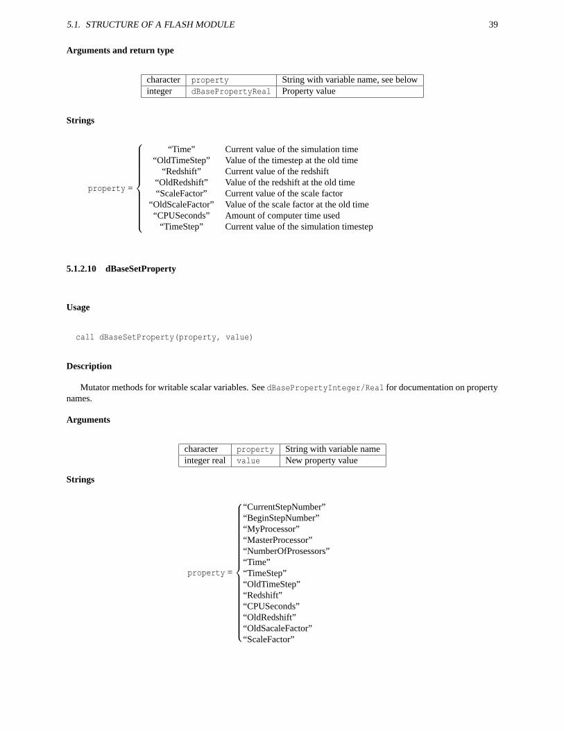
5.1. STRUCTURE OF A FLASH MODULE 39
Arguments and return type
character property String with variable name, see belowinteger dBasePropertyReal Property value
Strings
property =
“Time” Current value of the simulation time“OldTimeStep” Value of the timestep at the old time
“Redshift” Current value of the redshift“OldRedshift” Value of the redshift at the old time“ScaleFactor” Current value of the scale factor
“OldScaleFactor” Value of the scale factor at the old time“CPUSeconds” Amount of computer time used
“TimeStep” Current value of the simulation timestep
5.1.2.10 dBaseSetProperty
Usage
call dBaseSetProperty(property, value)
Description
Mutator methods for writable scalar variables. See dBasePropertyInteger/Real for documentation on propertynames.
Arguments
character property String with variable nameinteger real value New property value
Strings
property =
“CurrentStepNumber”“BeginStepNumber”“MyProcessor”“MasterProcessor”“NumberOfProsessors”“Time”“TimeStep”“OldTimeStep”“Redshift”“CPUSeconds”“OldRedshift”“OldSacaleFactor”“ScaleFactor”
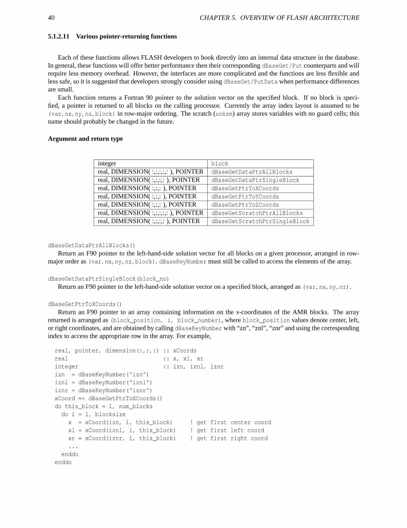
40 CHAPTER 5. OVERVIEW OF FLASH ARCHITECTURE
5.1.2.11 Various pointer-returning functions
Each of these functions allows FLASH developers to hook directly into an internal data structure in the database.In general, these functions will offer better performance then their corresponding dBaseGet/Put counterparts and willrequire less memory overhead. However, the interfaces are more complicated and the functions are less flexible andless safe, so it is suggested that developers strongly consider using dBaseGet/PutData when performance differencesare small.
Each function returns a Fortran 90 pointer to the solution vector on the specified block. If no block is speci-fied, a pointer is returned to all blocks on the calling processor. Currently the array index layout is assumed to be(var,nx,ny,nz,block) in row-major ordering. The scratch (unksm) array stores variables with no guard cells; thisname should probably be changed in the future.
Argument and return type
integer blockreal, DIMENSION( :,:,:,:,: ), POINTER dBaseGetDataPtrAllBlocksreal, DIMENSION( :,:,:,: ), POINTER dBaseGetDataPtrSingleBlockreal, DIMENSION( :,:,: ), POINTER dBaseGetPtrToXCoordsreal, DIMENSION( :,:,: ), POINTER dBaseGetPtrToYCoordsreal, DIMENSION( :,:,: ), POINTER dBaseGetPtrToZCoordsreal, DIMENSION( :,:,:,:,: ), POINTER dBaseGetScratchPtrAllBlocksreal, DIMENSION( :,:,:,: ), POINTER dBaseGetScratchPtrSingleBlock
dBaseGetDataPtrAllBlocks()Return an F90 pointer to the left-hand-side solution vector for all blocks on a given processor, arranged in row-
major order as (var,nx,ny,nz,block). dBaseKeyNumber must still be called to access the elements of the array.
dBaseGetDataPtrSingleBlock(block_no)Return an F90 pointer to the left-hand-side solution vector on a specified block, arranged as (var,nx,ny,nz).
dBaseGetPtrToXCoords()Return an F90 pointer to an array containing information on the x-coordinates of the AMR blocks. The array
returned is arranged as (block_position, i, block_number), where block_position values denote center, left,or right coordinates, and are obtained by calling dBaseKeyNumber with “zn”, “znl”, “znr” and using the correspondingindex to access the appropriate row in the array. For example,
real, pointer, dimension(:,:,:) :: xCoordsreal :: x, xl, xrinteger :: izn, iznl, iznrizn = dBaseKeyNumber("izn")iznl = dBaseKeyNumber("iznl")iznr = dBaseKeyNumber("iznr")xCoord => dBaseGetPtrToXCoords()do this_block = 1, num_blocksdo i = 1, blocksizex = xCoord(izn, i, this_block) ! get first center coordxl = xCoord(iznl, i, this_block) ! get first left coordxr = xCoord(iznr, i, this_block) ! get first right coord...
enddoenddo
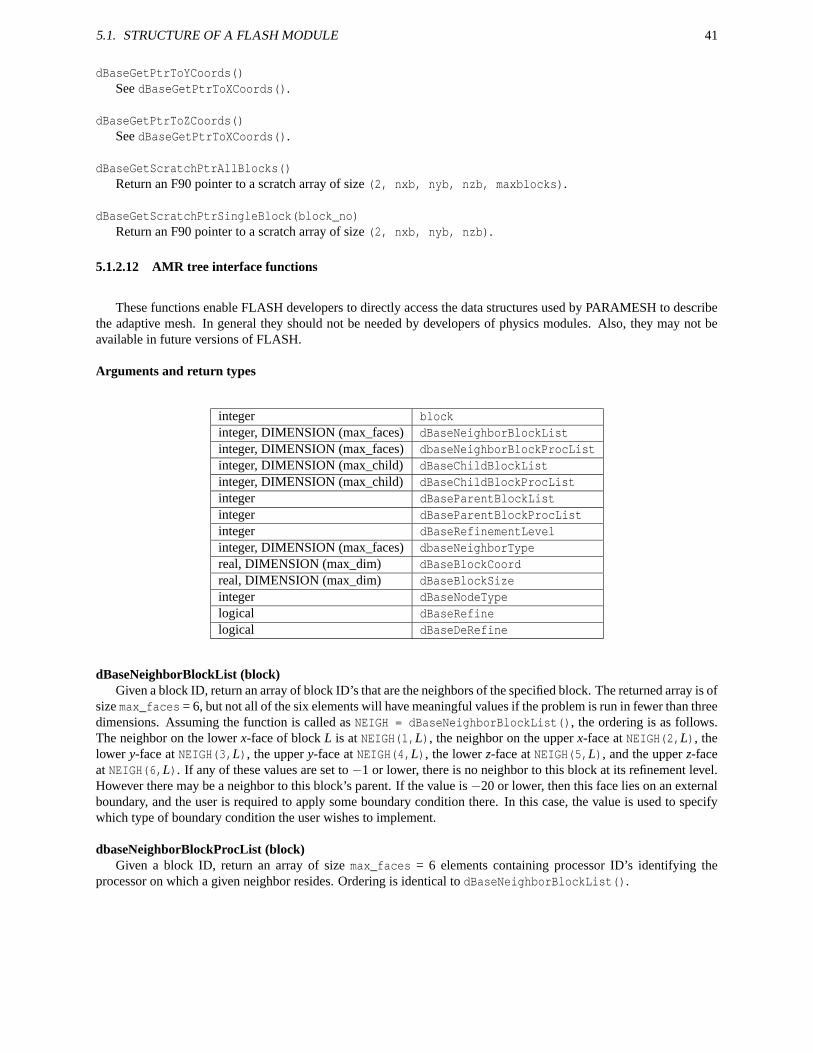
5.1. STRUCTURE OF A FLASH MODULE 41
dBaseGetPtrToYCoords()See dBaseGetPtrToXCoords().
dBaseGetPtrToZCoords()See dBaseGetPtrToXCoords().
dBaseGetScratchPtrAllBlocks()Return an F90 pointer to a scratch array of size (2, nxb, nyb, nzb, maxblocks).
dBaseGetScratchPtrSingleBlock(block_no)Return an F90 pointer to a scratch array of size (2, nxb, nyb, nzb).
5.1.2.12 AMR tree interface functions
These functions enable FLASH developers to directly access the data structures used by PARAMESH to describethe adaptive mesh. In general they should not be needed by developers of physics modules. Also, they may not beavailable in future versions of FLASH.
Arguments and return types
integer blockinteger, DIMENSION (max_faces) dBaseNeighborBlockListinteger, DIMENSION (max_faces) dbaseNeighborBlockProcListinteger, DIMENSION (max_child) dBaseChildBlockListinteger, DIMENSION (max_child) dBaseChildBlockProcListinteger dBaseParentBlockListinteger dBaseParentBlockProcListinteger dBaseRefinementLevelinteger, DIMENSION (max_faces) dbaseNeighborTypereal, DIMENSION (max_dim) dBaseBlockCoordreal, DIMENSION (max_dim) dBaseBlockSizeinteger dBaseNodeTypelogical dBaseRefinelogical dBaseDeRefine
dBaseNeighborBlockList (block)Given a block ID, return an array of block ID’s that are the neighbors of the specified block. The returned array is of
size max_faces = 6, but not all of the six elements will have meaningful values if the problem is run in fewer than threedimensions. Assuming the function is called as NEIGH = dBaseNeighborBlockList(), the ordering is as follows.The neighbor on the lower x-face of block L is at NEIGH(1,L), the neighbor on the upper x-face at NEIGH(2,L), thelower y-face at NEIGH(3,L), the upper y-face at NEIGH(4,L), the lower z-face at NEIGH(5,L), and the upper z-faceat NEIGH(6,L). If any of these values are set to −1 or lower, there is no neighbor to this block at its refinement level.However there may be a neighbor to this block’s parent. If the value is −20 or lower, then this face lies on an externalboundary, and the user is required to apply some boundary condition there. In this case, the value is used to specifywhich type of boundary condition the user wishes to implement.
dbaseNeighborBlockProcList (block)Given a block ID, return an array of size max_faces = 6 elements containing processor ID’s identifying the
processor on which a given neighbor resides. Ordering is identical to dBaseNeighborBlockList().
42 CHAPTER 5. OVERVIEW OF FLASH ARCHITECTURE
dBaseChildBlockList (block)Given a block ID, return an array of size max_child = 2 * max_dim elements containing the block ID’s of the
child blocks of the specified block. The children of a parent are numbered according to the Fortran array orderingconvention, i.e. child 1 is at the lower x, y, and z corner of the parent, child 2 at the higher x coordinate but lower y andz, child 3 at lower x, higher y and lower z, child 4 at higher x and y and lower z, and so on.
dBaseChildBlockProcList (block)Given a block ID, return an array of size max_child elements containing processor ID’s of the children of the
specified block. Ordering is identical to dBaseChildBlockList().
dBaseParentBlockList (block)Given a block ID, return the ID of the block’s parent block.
dBaseParentBlockProcList (block)Given a block ID, return the processor ID upon which the block’s parent resides.
dBaseRefinementLevel (block)Given a block ID, return that block’s integer level of refinement.
dBaseNodeType (block)Given a block ID, return the block’s node type. If the node type is 1, then the node is a leaf node. If it is 2, then
the node is a parent with at least 1 leaf child. Otherwise, it is set to 3 and does not have any up-to-date data.
dbaseNeighborType (block)Given a block ID, return an array of size (max_faces, maxblocks_tr) containing the type ID’s of the neighbors
of the specified block. max_faces = max_dim * 2, where max_dim is the maximum possible dimensionality (3).
dBaseBlockCoord (block)Given a block ID, return an array of size max_dim containing the x-,y-,and z-coordinates of the center of the block.
dBaseBlockSize (block)Given a block ID, return an array of size max_dim containing the block size in the x-, y-, and z-directions.
dBaseRefine (block)Given a block ID, return .true., if that block is set for refinement when amr_refine_derefine() is called next
and .false. otherwise.
dBaseDeRefine (block)Given a block ID, return .true., if that block is set to be derefined when amr_refine_derefine() is called next
and .false. otherwise.
5.1.3 Algorithms
Within each module is one or more procedures that perform the bulk of the computational work for the module.A principal strategy behind the FLASH architecture is to decouple these procedures as much as possible from thedetails of the framework in which they are embedded. This is accomplished by requiring that all module algorithmscommunicate data only through function argument lists. That is, algorithms may not query the database directly normay they depend on the existence of externally defined or global variables. This design ensures that algorithms can betested, developed, and interchanged in complete isolation from the larger, more complicated framework.
Thus, each algorithm in a module should have a well-defined argument list. It is up to the algorithm developer tomake this as general or restrictive as he/she sees fit. However, it is important to keep in mind that the more rigid theargument list, the less chance that another algorithm can share its interface. The consequence is that the developerwould have to add an entirely new wrapper function for just slightly different functionality.
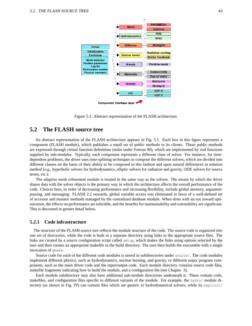
5.2. THE FLASH SOURCE TREE 43
Figure 5.1: Abstract representation of the FLASH architecture.
5.2 The FLASH source tree
An abstract representation of the FLASH architecture appears in Fig. 5.1. Each box in this figure represents acomponent (FLASH module), which publishes a small set of public methods to its clients. These public methodsare expressed through virtual function definitions (stubs under Fortran 90), which are implemented by real functionssupplied by sub-modules. Typically, each component represents a different class of solver. For instance, for time-dependent problems, the driver uses time-splitting techniques to compose the different solvers, which are divided intodifferent classes on the basis of their ability to be composed in this fashion and upon natural differences in solutionmethod (e.g., hyperbolic solvers for hydrodynamics, elliptic solvers for radiation and gravity, ODE solvers for sourceterms, etc.).
The adaptive mesh refinement module is treated in the same way as the solvers. The means by which the drivershares data with the solver objects is the primary way in which the architecture affects the overall performance of thecode. Choices here, in order of decreasing performance and increasing flexibility, include global memory, argument-passing, and messaging. FLASH 2.2 onwards, global variable access was eliminated in favor of a well-defined setof accessor and mutator methods managed by the centralized database module. When done with an eye toward opti-mization, the effects on performance are tolerable, and the benefits for maintainability and extensibility are significant.This is discussed in greater detail below.
5.2.1 Code infrastructure
The structure of the FLASH source tree reflects the module structure of the code. The source code is organized intoone set of directories, while the code is built in a separate directory using links to the appropriate source files. Thelinks are created by a source configuration script called setup, which makes the links using options selected by theuser and then creates an appropriate makefile in the build directory. The user then builds the executable with a singleinvocation of gmake.
Source code for each of the different code modules is stored in subdirectories under source/. The code modulesimplement different physics, such as hydrodynamics, nuclear burning, and gravity, or different major program com-ponents, such as the main driver code and the input/output code. Each module directory contains source code files,makefile fragments indicating how to build the module, and a configuration file (see Chapter 3).
Each module subdirectory may also have additional sub-module directories underneath it. These contain code,makefiles, and configuration files specific to different variants of the module. For example, the hydro/ module di-rectory (as shown in Fig. ??) can contain files which are generic to hydrodynamical solvers, while its explicit/
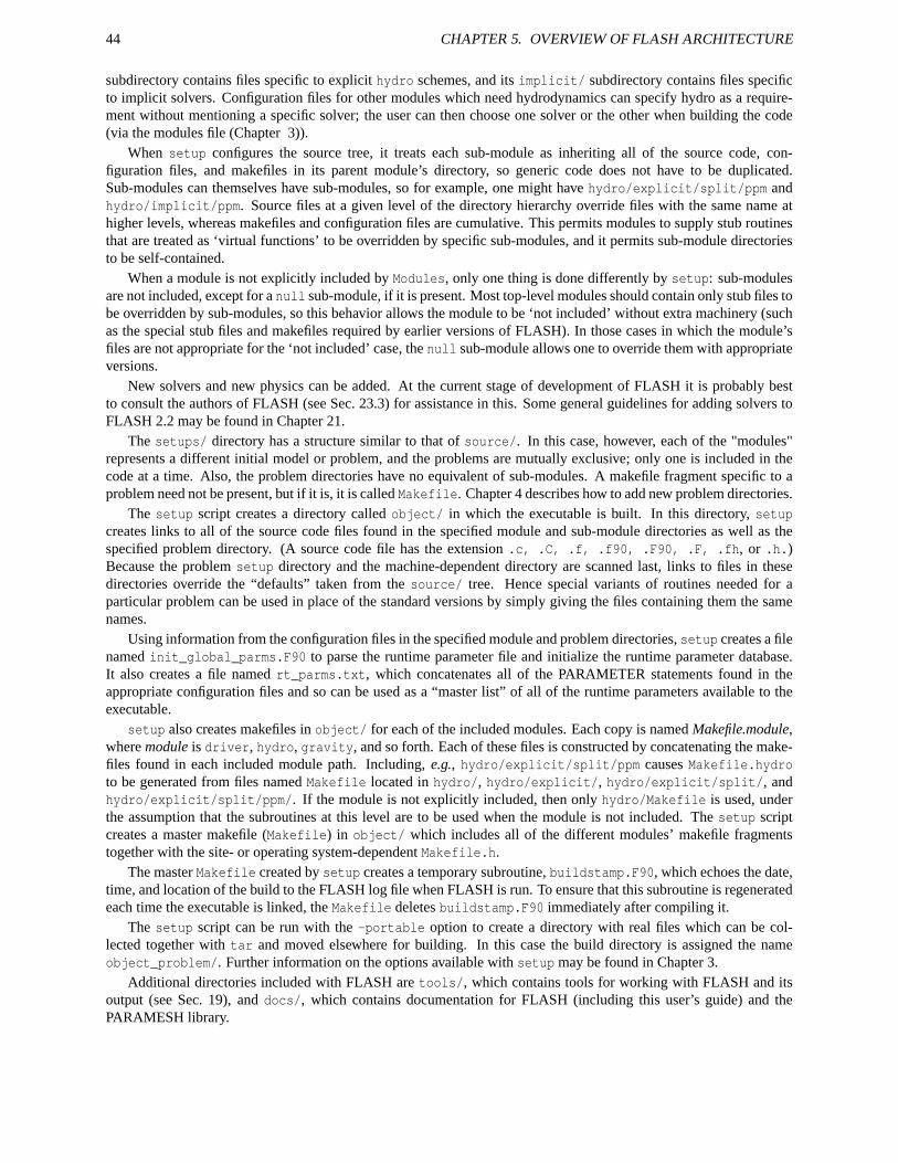
44 CHAPTER 5. OVERVIEW OF FLASH ARCHITECTURE
subdirectory contains files specific to explicit hydro schemes, and its implicit/ subdirectory contains files specificto implicit solvers. Configuration files for other modules which need hydrodynamics can specify hydro as a require-ment without mentioning a specific solver; the user can then choose one solver or the other when building the code(via the modules file (Chapter 3)).
When setup configures the source tree, it treats each sub-module as inheriting all of the source code, con-figuration files, and makefiles in its parent module’s directory, so generic code does not have to be duplicated.Sub-modules can themselves have sub-modules, so for example, one might have hydro/explicit/split/ppm andhydro/implicit/ppm. Source files at a given level of the directory hierarchy override files with the same name athigher levels, whereas makefiles and configuration files are cumulative. This permits modules to supply stub routinesthat are treated as ‘virtual functions’ to be overridden by specific sub-modules, and it permits sub-module directoriesto be self-contained.
When a module is not explicitly included by Modules, only one thing is done differently by setup: sub-modulesare not included, except for a null sub-module, if it is present. Most top-level modules should contain only stub files tobe overridden by sub-modules, so this behavior allows the module to be ‘not included’ without extra machinery (suchas the special stub files and makefiles required by earlier versions of FLASH). In those cases in which the module’sfiles are not appropriate for the ‘not included’ case, the null sub-module allows one to override them with appropriateversions.
New solvers and new physics can be added. At the current stage of development of FLASH it is probably bestto consult the authors of FLASH (see Sec. 23.3) for assistance in this. Some general guidelines for adding solvers toFLASH 2.2 may be found in Chapter 21.
The setups/ directory has a structure similar to that of source/. In this case, however, each of the "modules"represents a different initial model or problem, and the problems are mutually exclusive; only one is included in thecode at a time. Also, the problem directories have no equivalent of sub-modules. A makefile fragment specific to aproblem need not be present, but if it is, it is called Makefile. Chapter 4 describes how to add new problem directories.
The setup script creates a directory called object/ in which the executable is built. In this directory, setupcreates links to all of the source code files found in the specified module and sub-module directories as well as thespecified problem directory. (A source code file has the extension .c, .C, .f, .f90, .F90, .F, .fh, or .h.)Because the problem setup directory and the machine-dependent directory are scanned last, links to files in thesedirectories override the “defaults” taken from the source/ tree. Hence special variants of routines needed for aparticular problem can be used in place of the standard versions by simply giving the files containing them the samenames.
Using information from the configuration files in the specified module and problem directories, setup creates a filenamed init_global_parms.F90 to parse the runtime parameter file and initialize the runtime parameter database.It also creates a file named rt_parms.txt, which concatenates all of the PARAMETER statements found in theappropriate configuration files and so can be used as a “master list” of all of the runtime parameters available to theexecutable.
setup also creates makefiles in object/ for each of the included modules. Each copy is named Makefile.module,where module is driver, hydro, gravity, and so forth. Each of these files is constructed by concatenating the make-files found in each included module path. Including, e.g., hydro/explicit/split/ppm causes Makefile.hydroto be generated from files named Makefile located in hydro/, hydro/explicit/, hydro/explicit/split/, andhydro/explicit/split/ppm/. If the module is not explicitly included, then only hydro/Makefile is used, underthe assumption that the subroutines at this level are to be used when the module is not included. The setup scriptcreates a master makefile (Makefile) in object/ which includes all of the different modules’ makefile fragmentstogether with the site- or operating system-dependent Makefile.h.
The master Makefile created by setup creates a temporary subroutine, buildstamp.F90, which echoes the date,time, and location of the build to the FLASH log file when FLASH is run. To ensure that this subroutine is regeneratedeach time the executable is linked, the Makefile deletes buildstamp.F90 immediately after compiling it.
The setup script can be run with the -portable option to create a directory with real files which can be col-lected together with tar and moved elsewhere for building. In this case the build directory is assigned the nameobject_problem/. Further information on the options available with setup may be found in Chapter 3.
Additional directories included with FLASH are tools/, which contains tools for working with FLASH and itsoutput (see Sec. 19), and docs/, which contains documentation for FLASH (including this user’s guide) and thePARAMESH library.

5.3. MODULES INCLUDED WITH FLASH: A BRIEF OVERVIEW 45
5.3 Modules included with FLASH: a brief overview
The current FLASH distribution comes with a set of core components that form the backbone of many commonproblems, namely database, driver, hydro, io, mesh, particles, source_terms, gravity, and materials. A detailed discus-sion of the role of each of these modules is presented in Part IV. Here we give a brief overview of each.
Chapter 6 describes in detail the various driver modules that may be implemented with FLASH. In addition tothe default driver, which controls the initialization, evolution, and output of a FLASH simulation, four new drivermodules have been written to implement different explicit time advancement algorithms. Three are written in the deltaformulation: euler1, rk3, and strang_delta. The fourth, strang_state, is written in the state-vector formulation.This chapter also includes a subsection concerning simulation services, runtime parameters, and logfiles.
Chapter 7 describes the FLASH I/O modules, which control how FLASH data structures are stored on differentplatforms and in different formats. Discussed in this section are the I/O modules hdf5_serial and hdf5_parallel,which use the Hierarchical Data Format (HDF) for storing simulation data, PnetCDF which uses parallel netCDF I/Olibrary, and is new in FLASH 2.5. There is also discussion of the legacy hdf4 I/O module, which is no longer activelysupported.
Chapter 8 describes the mesh module, together with the PARAMESH package of subroutines for the parallelizationand adaptive mesh refinement (AMR) portion of FLASH.
Chapter 9 describes the two hydrodynamic modules included in FLASH 2. The first is based on the PROMETHEUScode (Fryxell, Müller, and Arnett 1989); the second is based on Kurganov numerical methods. Sec. 9.3 is a discussionof the relativistic hydrodynamics module, which is new in FLASH 2.5. Sec. 9.4 describes the magnetohydrodynamicsmodule included with the FLASH code.
Chapter 10 discusses the material properties module, which handles the tracking of multiple fluids in FLASHsimulations. It includes the equation of state module, which implements the EOS for the hydrodynamical and nuclearburning solvers; the composition submodule, which sets up the different compositions needed by FLASH; and thestellar conductivity module, which may be used for computing the opacity of stellar material.
Chapter 11 describes various source terms, including the nuclear burning module, which calculates the nuclearburning rate during a hydrodynamical simulation, and the stirring module, which adds a divergence-free, time-correlated ‘stirring’ velocity at selected modes in a given hydrodynamical simulation. Also included are modulesfor ionization, heating, and cooling.
Chapter 12 describes the gravity module, which computes the gravitational potential or gravitational accelerationsource terms for the code. It includes several sub-modules: the constant submodule, the plane parallel sub-module,the ptmass submodule, and the Poisson submodules.
Chapter 13 describes the particle module, which follows the evolution of both physical particles and Lagrangianmass tracers.
Chapter 14 describes the cosmology module, which provides features required for solving cosmological problemsin comoving coordinates. These include the evolution of the scale factor (via the Friedmann equation), the redshiftterms in the comoving Euler equations, and a library of useful cosmological functions (e.g., to convert redshifts totimes).
Chapter 15 describes several solvers included with FLASH, including solvers for ordinary differential equations(ODE) and multipole and multigrid Poisson solvers.
Chapter 16 describes the 2d runtime visualization module used to produce simple pictures of a FLASH simulation.Finally, Chapter 17 describes the utilities module, which is a collection of reusable high-level utility functions that
simplify programming in FLASH.

46 CHAPTER 5. OVERVIEW OF FLASH ARCHITECTURE
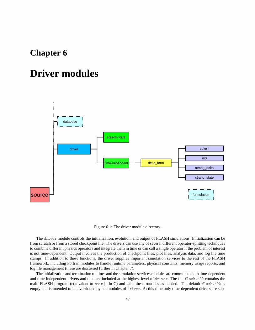
Chapter 6
Driver modules
Figure 6.1: The driver module directory.
The driver module controls the initialization, evolution, and output of FLASH simulations. Initialization can befrom scratch or from a stored checkpoint file. The drivers can use any of several different operator-splitting techniquesto combine different physics operators and integrate them in time or can call a single operator if the problem of interestis not time-dependent. Output involves the production of checkpoint files, plot files, analysis data, and log file timestamps. In addition to these functions, the driver supplies important simulation services to the rest of the FLASHframework, including Fortran modules to handle runtime parameters, physical constants, memory usage reports, andlog file management (these are discussed further in Chapter 7).
The initialization and termination routines and the simulation services modules are common to both time-dependentand time-independent drivers and thus are included at the highest level of driver. The file flash.F90 contains themain FLASH program (equivalent to main() in C) and calls these routines as needed. The default flash.F90 isempty and is intended to be overridden by submodules of driver. At this time only time-dependent drivers are sup-
47
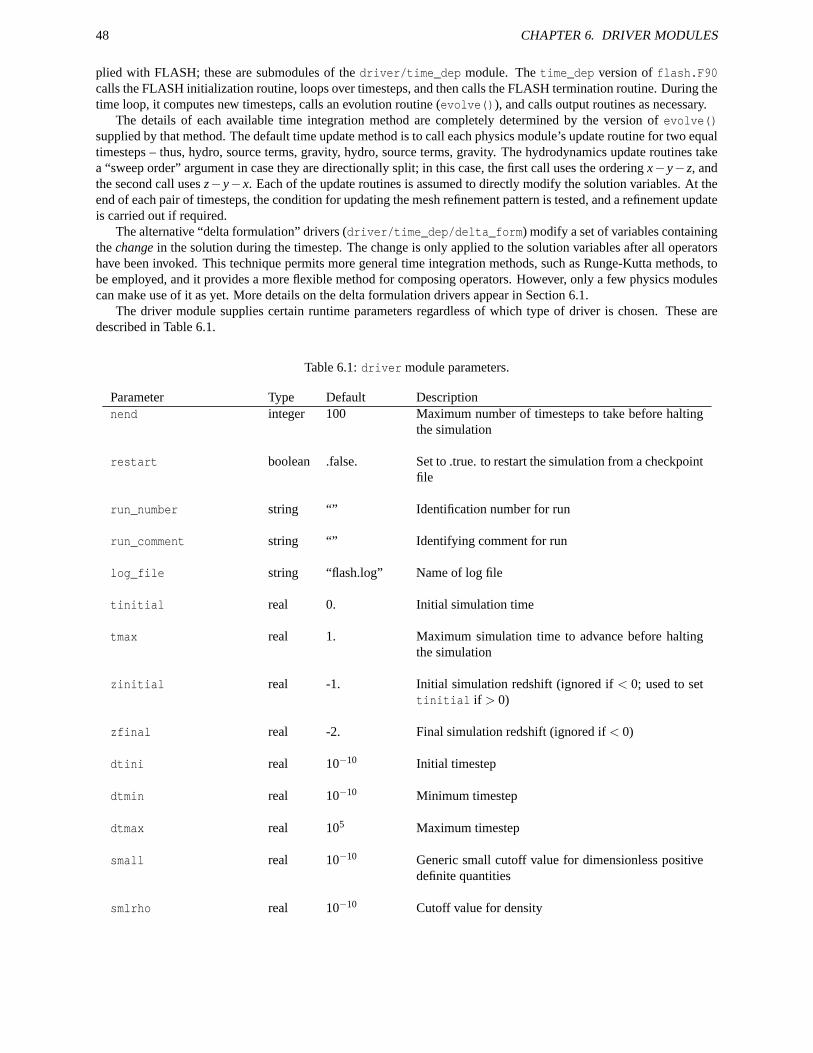
48 CHAPTER 6. DRIVER MODULES
plied with FLASH; these are submodules of the driver/time_dep module. The time_dep version of flash.F90calls the FLASH initialization routine, loops over timesteps, and then calls the FLASH termination routine. During thetime loop, it computes new timesteps, calls an evolution routine (evolve()), and calls output routines as necessary.
The details of each available time integration method are completely determined by the version of evolve()supplied by that method. The default time update method is to call each physics module’s update routine for two equaltimesteps – thus, hydro, source terms, gravity, hydro, source terms, gravity. The hydrodynamics update routines takea “sweep order” argument in case they are directionally split; in this case, the first call uses the ordering x− y− z, andthe second call uses z− y− x. Each of the update routines is assumed to directly modify the solution variables. At theend of each pair of timesteps, the condition for updating the mesh refinement pattern is tested, and a refinement updateis carried out if required.
The alternative “delta formulation” drivers (driver/time_dep/delta_form) modify a set of variables containingthe change in the solution during the timestep. The change is only applied to the solution variables after all operatorshave been invoked. This technique permits more general time integration methods, such as Runge-Kutta methods, tobe employed, and it provides a more flexible method for composing operators. However, only a few physics modulescan make use of it as yet. More details on the delta formulation drivers appear in Section 6.1.
The driver module supplies certain runtime parameters regardless of which type of driver is chosen. These aredescribed in Table 6.1.
Table 6.1: driver module parameters.
Parameter Type Default Descriptionnend integer 100 Maximum number of timesteps to take before halting
the simulation
restart boolean .false. Set to .true. to restart the simulation from a checkpointfile
run_number string “” Identification number for run
run_comment string “” Identifying comment for run
log_file string “flash.log” Name of log file
tinitial real 0. Initial simulation time
tmax real 1. Maximum simulation time to advance before haltingthe simulation
zinitial real -1. Initial simulation redshift (ignored if < 0; used to settinitial if > 0)
zfinal real -2. Final simulation redshift (ignored if < 0)
dtini real 10−10 Initial timestep
dtmin real 10−10 Minimum timestep
dtmax real 105 Maximum timestep
small real 10−10 Generic small cutoff value for dimensionless positivedefinite quantities
smlrho real 10−10 Cutoff value for density
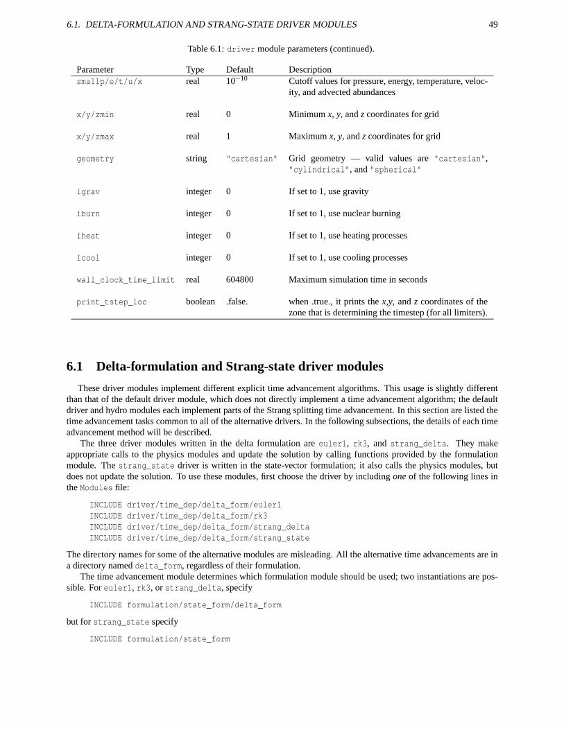
6.1. DELTA-FORMULATION AND STRANG-STATE DRIVER MODULES 49
Table 6.1: driver module parameters (continued).
Parameter Type Default Descriptionsmallp/e/t/u/x real 10−10 Cutoff values for pressure, energy, temperature, veloc-
ity, and advected abundances
x/y/zmin real 0 Minimum x, y, and z coordinates for grid
x/y/zmax real 1 Maximum x, y, and z coordinates for grid
geometry string "cartesian" Grid geometry — valid values are "cartesian","cylindrical", and "spherical"
igrav integer 0 If set to 1, use gravity
iburn integer 0 If set to 1, use nuclear burning
iheat integer 0 If set to 1, use heating processes
icool integer 0 If set to 1, use cooling processes
wall_clock_time_limit real 604800 Maximum simulation time in seconds
print_tstep_loc boolean .false. when .true., it prints the x,y, and z coordinates of thezone that is determining the timestep (for all limiters).
6.1 Delta-formulation and Strang-state driver modules
These driver modules implement different explicit time advancement algorithms. This usage is slightly differentthan that of the default driver module, which does not directly implement a time advancement algorithm; the defaultdriver and hydro modules each implement parts of the Strang splitting time advancement. In this section are listed thetime advancement tasks common to all of the alternative drivers. In the following subsections, the details of each timeadvancement method will be described.
The three driver modules written in the delta formulation are euler1, rk3, and strang_delta. They makeappropriate calls to the physics modules and update the solution by calling functions provided by the formulationmodule. The strang_state driver is written in the state-vector formulation; it also calls the physics modules, butdoes not update the solution. To use these modules, first choose the driver by including one of the following lines inthe Modules file:
INCLUDE driver/time_dep/delta_form/euler1INCLUDE driver/time_dep/delta_form/rk3INCLUDE driver/time_dep/delta_form/strang_deltaINCLUDE driver/time_dep/delta_form/strang_state
The directory names for some of the alternative modules are misleading. All the alternative time advancements are ina directory named delta_form, regardless of their formulation.
The time advancement module determines which formulation module should be used; two instantiations are pos-sible. For euler1, rk3, or strang_delta, specify
INCLUDE formulation/state_form/delta_form
but for strang_state specify
INCLUDE formulation/state_form
50 CHAPTER 6. DRIVER MODULES
The services provided by the formulation module for the delta formulation are a superset of those provided for thestate-vector formulation, which explains the directory structure used. For both instantiations, the formulation modulecontains (i) subroutines for updating the conserved and auxiliary variables locally (on a block or on a face of a block)given a local operator Lphysics(U) and (ii) a parameter which declares which formulation is being used. For thedelta formulation, the module also (iii) declares the global ∆U array and contains subroutines for accessing it and(iv) provides a subroutine to update the variables globally.
For delta formulation time advancements, the delta formulation driver modules use the formulation module to holdand access the global ∆U array and to update the solution. In the state-vector formulation, the formulation module isnot directly used by the driver; instead, the physics modules call the update subroutines that the formulation moduleprovides.
The alternative driver modules discretize the left-hand side of
∂V∂t
= (spatial difference terms)+(source terms) . (6.1)
The time advancement algorithm is contained in a subroutine named evolve. Each call to evolve advances thesolution through one timestep for the euler1 and rk3 modules and through two timesteps for the strang_state andstrange_delta modules. Each time advancement algorithm begins with a vector of primary variables V n at time tn
and an associated set of auxiliary variables W n. Primarily through calls to other physics modules, evolve applies a setof operations to the variables to produce an updated vector V n+1 at time tn+1 = tn +∆t. Depending on the formulation,the time advancement may or may not update the auxiliary variables – in the state-vector formulation, the other physicsmodules update them.
The distinction between V and W is that time-dependent differential equations are solved to determine the primaryvariables. The auxiliary variables are obtained from the primary variables through algebraic relations. Often theprimary variables are the conserved variables U , and in the rest of this section, U will replace V . However, the timeadvancement algorithms implemented do not require this correspondence.
The time advancement algorithms are written generally, in that each differential equation is treated in the same way.The distinction between the equations (for example, between the x-momentum equation and the total energy equation)is expressed in the other physics modules. The time advancement algorithm does not need to know the identity of thevariables on which it operates, except possibly to update the auxiliary variables from the primary variables, but thisupdate is handled by a call to a subroutine provided by the formulation module.
6.1.1 The euler1 module
The euler1 module implements the first-order, Euler explicit scheme
Un+1 = Un +∆tL(Un) , (6.2)
where L(U) represents all of the physics modules. The Euler explicit method is implemented in the delta formulation.No runtime parameters are defined for this module.
At the beginning of a timestep, ∆U is set to zero. Each of the physics modules is called with U n as the initial stateand adds its contribution to ∆U . After all the physics modules have been called, the global ∆U array holds L(U n).Eq. (6.2) yields Un+1. Finally, the auxiliary variables are updated from the conserved variables with a call to the globalupdate subroutine provided by the formulation module.
Note that because all the physics modules start with the same initial state, the order in which the physics modulesare called does not affect the results (except possibly through floating point roundoff differences when contributing to∆U).
The set of steps, consisting of calls to physics modules, updating the conserved variables, and updating the auxiliaryvariables, is often called a stage. The majority of the computational cost of a stage is in the calls to the other physicsmodules; this component corresponds to a “function evaluation” for ordinary differential equation solvers. In the Eulerexplicit algorithm, there is one stage per timestep.
6.1.2 The rk3 module
Runge-Kutta schemes are a class of ordinary differential equation solvers which are appreciated for their higher orderof accuracy, ease of implementation, and relatively low storage requirements. There are many third-order Runge-Kutta
6.1. DELTA-FORMULATION AND STRANG-STATE DRIVER MODULES 51
methods; all require at least three stages. Most require at least three storage locations per primary variable, but the oneimplemented in the delta formulation in FLASH, derived by Williamson (J. Comp. Phys. 35:48, 1980), requires onlytwo.
The two storage registers will be referred to as U and ∆U . The global solution vector U holds U n at the beginningof the timestep and then intermediate solutions U (·) at the end of each stage. The manipulation of the global ∆U arrayis more complicated. ∆U accumulates contributions from the physics modules during a stage, but it also holds resultsfrom previous stages; it is important to distinguish between the results of the physics modules L(U) and the quantityheld in the global ∆U array. First the algorithm will be shown; then the usage of the global ∆U array will be discussed.For the equation
∂U∂t
= L(U) , (6.3)
Williamson’s algorithm is, starting with Un,
U (1) = Un +13
∆t[
L(Un)]
(6.4)
U (2) = U (1) +1516
∆t[
L(U (1))− 59
L(Un)]
(6.5)
Un+1 = U (3) = U (2) +8
15∆t[
L(U (2))− 153128
(
L(U (1))− 59
L(Un))]
. (6.6)
U (m) is the result of the m-th stage, and the auxiliary variables are updated each time a new U (m) is computed.The algorithm is implemented using the following steps to attain the low storage. At the beginning of the timestep,
∆U is set to zero. During the first stage each physics module contributes to ∆U , so after all have contributed, ∆U holdsthe bracketed term in eq. (6.4), L(Un). U (1) is then computed using eq. (6.4). Stage 1 is completed by multiplying ∆Uby −5/9, which is required for the following stages. The process is repeated for stage 2: after the physics moduleshave contributed, ∆U holds the bracketed term in eq. (6.5); U (2) is computed by eq. (6.5) and stored in U ; then ∆U ismultiplied by −153/128. Stage 3 is similar, but ends after U (3) = Un+1 is computed and stored. It is critical that theonly changes made to the ∆U array are those just listed; no physics module should change the value of ∆U , except toadd its contribution, and since ∆U holds information from previous stages, it should not be reset to zero except at thebeginning of the timestep. No runtime parameters are defined for this module.
6.1.3 strang_state and strang_delta modules
The second-order accurate splitting method (Strang 1968) is attractive because of its low memory requirements. Thealgorithm is based on the operator splitting approach, in which a set of simple subproblems is solved rather thana single, complicated problem. Each subproblem typically accounts for one term in a system of partial differentialequations, representing a particular type of physics for which an appropriate (specialized) numerical method is avail-able. If all the subproblems are computed to at least second-order accuracy, the basic operator splitting method isfirst-order accurate; however, the Strang splitting scheme recovers second-order accuracy over two timesteps. In thefirst timestep, the subproblems are solved in a given sequence. Second-order accuracy is obtained by reversing thesequence in the second timestep.
A key feature of the operator splitting approach is that the output of one subproblem is the input to the nextsubproblem. This allows for an implementation that globally, stores only the current solution, but it can also causeproblems including accuracy losses due to decoupling various physical effects (splitting errors) and difficulties imple-menting boundary conditions. In practice it has been found that splitting errors are reduced when the subproblemsare ordered in increasing stiffness, i.e. the stiffest subproblem is solved last in the sequence; this has recently beensupported by numerical analysis (Sportisse 2000).
Two driver modules implement an algorithm similar to the Strang splitting time advancement. Since the sequenceis not exactly reversed in the second step compared to the first, the algorithm is not the true Strang splitting. How-ever, the nuclear burning source terms are very stiff, and there are sound arguments for computing them last. Thestrang_state module implements the algorithm in the state-vector formulation and is recommended for “produc-tion” runs due to its low memory requirements. The strang_delta driver is implemented in the delta formulation andis provided for testing and comparison. For both versions, one call to evolve (which implements the time advancementalgorithm) advances the solution from tn to tn+2, i.e. over two timesteps.
In the strang_state driver, the sequence of calls to physics modules in the first timestep is
52 CHAPTER 6. DRIVER MODULES
hydro(x-sweep)hydro(y-sweep)hydro(z-sweep)gravitysource terms
In the second timestep, only the order of the hydro calls is reversed
hydro(z-sweep)hydro(y-sweep)hydro(x-sweep)gravitysource terms
Mesh refinement and derefinement are executed only after the second step, not between the two steps; also the timestepis held constant for the two steps. The y- and z-sweeps of hydro are not called unless that dimension is included in thesimulation. The same algorithm is used in the strang_delta module, but after each call to a physics module, a callto a subroutine is necessary to update the solution. When the strang_state driver is used, these calls are made byeach physics module. No runtime parameters are defined for either module.
6.1.4 The formulation modules
The purposes of this module class are
1. To provide functions usable by physics modules and driver modules to update the solution locally (on a blockor on a face of a block) or globally (on all blocks).
2. If needed by the time advancement (driver) module, to provide storage space for the global ∆U array andfunctions to access it.
The alternative time advancement methods (drivers) are implemented in either the state-vector or delta formulations.There are two corresponding instantiations of the formulation module. In the state-vector instantiation, only the localupdate functions in item (1) are provided; drivers in the state-vector formulation do not require any other services. Thedelta instantiation provides both local and global update functions and global ∆U array storage as required by driversin the delta formulation.
The services provided to delta formulation drivers are a superset of those provided to drivers in the state-vectorformulation, and the directory structure is used to express that. The /formulation/state_form directory con-tains the local update subroutines and a version of formulation_Module suitable for the state-vector instantia-tion. formulation_Module defines a module in the Fortran90 sense as opposed to the FLASH hierarchy sense.The formulation/state_form/delta_form directory contains the global update subroutine and the version offormulation_Module required for the delta instantiation.
When /formulation/state_form is specified in the Modules file, the local update functions and the first formulation_Moduleare built into the executable, as appropriate for drivers in the state-vector formulation; when /formulation/state_form/delta_formis specified in the Modules file, the local update functions, the global update function, and the second version offormulation_Module are used in the executable, as required by drivers in the delta formulation. This use of theFLASH code framework and directory hierarchy allows static allocation of the global ∆U array when needed butsaves that memory when not. At the same time, it allows local update functions to be used by both state-vector anddelta formulations without duplicating code.
Currently the update functions apply only to the particular variable sets described. The local update functionsmust be given the (old) conserved variables in the order ρ1, · · · ,ρionmax, ρu, ρv, ρw, ρE, and they store in the databaseX1, · · · ,Xionmax, ρ, P, T , γ, u, v, w, and E. The mapping from the conserved variables to the database variables is notgeneral; it is specific to the variables just listed. Variables other than those specifically listed will not be updated, andtheir influence on the variables just listed will be ignored. Development of more flexible update routines is underway.However, changes will most likely be internal to the local and global update functions, and the organization of thesemodules is not expected to change.
6.1. DELTA-FORMULATION AND STRANG-STATE DRIVER MODULES 53
6.1.4.1 State-Vector Instantiation
In this subsection the local update functions, named du_update_block, du_update_xface, du_update_yface,and du_update_zface, are described. These subroutines accept local arrays of conserved variables and their changesas inputs, compute updated conserved variables, compute auxiliary variables from algebraic relations (with the aid ofappropriate equation of state calls), and store the updated variables in the database.
These subroutines accept the block number, a local ∆U , local conserved variables U , the timestep ∆t, and a scalarfactor c, all as passed arguments. The face update routines also accept an index specifying which grid plane to update.The conserved variables are updated by
Unew = Uold + c∆t∆U . (6.7)
The factor c allows an update to an intermediate time between tn and tn+1, often required by Runge-Kutta timeadvancement methods; it is intended for use by drivers in the delta formulation through the global update subroutine.
From the updated conserved variables, all variables stored in the database are computed. The density ρ and speciesmass fractions Xs are obtained from the species densities ρs. The velocity components u, v, and w and the total energyper unit mass E are computed from the momenta and total energy per unit volume, respectively, by dividing by ρ.The internal energy ε is calculated by subtracting the kinetic energy per unit mass (u2 + v2 + w2)/2 from E. Thetemperature T , pressure P, and ratio of specific heats γ are obtained through a call to the equation of state, for whichρ, Xs, and ε are inputs.
Finally, the updated variables are stored in the variable database. The variables stored are Xs, ρ, P, T , γ, u, v, w, andE. Only the interior cells of a block or face are updated; for all guard cells, zeros are stored for all updated variables.None of the calculations described above are executed for the guard cells.
For the state-vector formulation, there are only a few tasks for the Fortran 90 module formulation_Module. First,it defines a Fortran logical parameter delta_formulation to be .false.. This parameter is designed to be accessedby physics modules. When .false., it indicates that each physics module should update the solution; while the localupdate routines just described are recommended for this purpose, there is no requirement that they be used. Second,formulation_Module defines several parameters for sizing arrays and a set of integers (indices) used to access thevariable database; these are used by the local update subroutines.
In the state-vector instantiation, formulation_Module does not declare the global ∆U array. It does define somefunctions which are used to access that array, but in this instantiation they do not perform any operations – they are‘stub’ functions. The reason for defining them is as follows. If a physics module is written so that either the state-vectoror delta formulation can be used, it must include calls to functions which give access to the global ∆U array. When thestate-vector formulation is used these calls are not made, but many compilers raise errors when these functions are notdefined. By defining them in this instantiation of formulation_Module, such errors are avoided. The stub functionsare contained, in the Fortran 90 sense, in formulation_Module. The local update functions are not contained informulation_Module, although they directly access the array sizing parameters and database indices therein.
6.1.4.2 Delta Instantiation
In this section the global update subroutine du_update and the version of formulation_Module used for the deltaformulation are described. The global update routine is a wrapper to the local update subroutine du_update_block.Two arguments, c and ∆t, are passed into du_update. For each block, it gets ρ, Xs, u, v, w, and E from the database;computes the (old) conserved variables from these; gets the ∆U for the block from the global ∆U array; and callsdu_update_block. Recall that du_update_block computes the updated variables and stores them in the database.
For the delta instantiation, formulation_Module defines the same array-sizing parameters and database in-dices as in the state-vector instantiation. However, it defines the parameter delta_formulation to be .true.,indicating to the physics modules that their contributions should be added to the global ∆U array. The delta in-stantiation of formulation_Module statically allocates the global ∆U array and defines several functions to ma-nipulate it. Each element of the global ∆U array is set to zero by du_zero. A physics module can add its lo-cal ∆U for a block to the global array by calling du_block_to_global; the subroutines du_xface_to_global,du_yface_to_global and du_zface_to_global do the same for faces (slices) of a block. These subroutines arecontained in formulation_Module and are the actual, working versions of the stub functions defined in the state-vector instantiation.
The global ∆U array is a public, module-scope variable in the Fortran 90 sense. The du_update subroutine is notcontained in formulation_Module but can access the array-sizing parameters and database indices in the module. It
54 CHAPTER 6. DRIVER MODULES
can also access the global ∆U array directly and is the only subroutine not contained in formulation_Module allowedto do so.
6.2 Simulation services
6.2.1 Runtime parameters
The driver module provides a Fortran 90 module called runtime_parameters. The routines in this module maintain‘parameter contexts,’ essentially small databases of runtime parameters. Contexts can be created and destroyed, andruntime parameters can be added to them, have their values modified, and be queried as to their value or data type.These features allow a program to maintain several contexts for different code modules without having to declare andshare the parameters explicitly. User-written subroutines (e.g., for initialization) should use the routines in this moduleto access the values of any runtime parameters they require.
An example of the application of this module is to use the read_parameters() routine (separately supplied) toparse a text-format input file containing parameter settings. The calling program declares a context, adds parametersto it, and then calls read_parameters() to parse the input file. Finally, the context is queried to obtain the inputvalues. Such a program might look like the following code fragment.
program testuse runtime_parameterstype (parm_context_type) :: contextreal :: x_init...call create_parm_context (context)call add_parm_to_context (context, "x_init", 4.)...call read_parameters ("input.par", context)call get_parm_from_context (context, "x_init", x_init)...end
Parameter names supplied as arguments to the routines are stored or compared in a case-insensitive fashion. Thus N_xand n_x refer to the same parameter, and
integer n_xcall add_parm_to_context (context, "N_x", 32)call get_parm_from_context (context, "n_X", n_x)write (*,*) n_xcall set_parm_in_context (context, "n_x", 64)call get_parm_from_context (context, "N_X", n_x)write (*,*) n_x
prints
3264
The following routines, data types, and public constants are provided by this module. Note that the main FLASHinitialization routine (init_flash()) and the initialization code created by setup already handle the creation of thedatabase and the parsing of the parameter file, so users will mainly be interested in querying the database for parametervalues.
• parm_context_type
Data type for contexts.
6.2. SIMULATION SERVICES 55
• global_parm_context
A parameter context available to all program units which use the runtime_parameters module. This is madeavailable only for programs that share the rest of their data among routines via included common blocks. Pro-grams which use modules should declare their own contexts within their modules.
• parm_real,int,str,log,invalid
Constants returned by get_parm_type_from_context().
• create_parm_context (c)
Create context c.
• destroy_parm_context (c)
Destroy context c, freeing up the memory occupied by its database.
• add_parm_to_context (c,p,v)
Add a parameter named p to context c. p is a character string naming the parameter, and v is the default or initialvalue to assign to the parameter. v can be of type real, integer, string, or logical. The type of v sets the type ofthe parameter; subsequent sets or gets of the parameter must be of the same type, or an error message will beprinted.
• set_parm_in_context (c,p,v)
Set the value of parameter p in context c equal to v. p is a character string naming the parameter, which mustalready have been created by add_parm_to_context (else an error message is printed). The type of v mustmatch the type of the initial value used to create the parameter, else an error message is printed.
• get_parm_from_context (c,p,v)
Query context c for the value of parameter p and return this value in the variable v. Parameter p must alreadyexist, and the type of v must match the type of the initial value used to create the parameter, else an error messageis printed.
• get_parm_type_from_context (c,p,t)
Query context c for the data type of parameter p. The result is returned in t, which must be of type integer.Possible return values are parm_real, parm_int, parm_str, parm_log, and parm_invalid. parm_invalidis returned if the named parameter does not exist.
• list_parm_context (c,l)
Print (to I/O unit l) the names and values of all parameters associated with context c.
• bcast_parm_context (c,p,r)
Broadcast the parameter names and values from a specified context c to all processors. p is the calling processor’srank, and r is the rank of the root processor (the one doing the broadcasting).
6.2.2 Physical constants
The driver supplies a Fortran 90 module called physical_constants, which maintains a centralized database ofphysical constants. The database can be queried by string name and optionally converted to any chosen system ofunits. The default system of units is CGS. This facility makes it easy to ensure that all parts of the code are usinga consistent set of physical constant values and unit conversions and to update the constants used by the code asimproved measurements become available.
For example, a program using this module might obtain the value of Newton’s gravitational constant G in units ofMpc3 Gyr−2 M−1
by calling
call get_constant_from_db ("Newton", G, len_unit="Mpc",time_unit="Gyr", mass_unit="Msun")
56 CHAPTER 6. DRIVER MODULES
In this example, the local variable G is set equal to the result, 4.4983×10⁻¹⁵ (to five significant figures).Physical constants are taken from the 1998 Review of Particle Properties, Eur. Phys. J. C 3, 1 (1998), which in
turn takes most of its values from Cohen, E. R. and Taylor, B. N., Rev. Mod. Phys. 59, 1121 (1987). The followingroutines are supplied by this module.
• get_constant_from_db (n,v[,units])
Return the value of the physical constant named n in the variable v. Optional unit specifications are used toconvert the result. If the constant name or one or more unit names aren’t recognized, a value of 0 is returned.
• add_constant_to_db (n,v,len,time,mass,temp,chg)
Add a physical constant to the database. n is the name to assign, and v is the value in CGS units. len, time,mass, temp, and chg are the exponents of the various base units used in defining the unit scaling of the constant.For example, a constant with units (in CGS) of cm3 s−2 g−1 would have len=3, time=-2, mass=-1, temp=0, andchg=0.
• add_unit_to_db (t,n,v)
Add a unit of measurement to the database. t is the type of unit (“length,” “time,” “mass,” “charge,” “tempera-ture”), n is the name of the unit, and v is its value in terms of the corresponding CGS unit. Compound units arenot supported, but they can be created as physical constants.
• init_constants_db ()
Initialize the constants and units databases. Can be called by the user program, but doesn’t have to be, since itis automatically called when needed (i.e. if a “get” or “add” is called before initialization).
• list_constants_db (lun)
List the constants and units databases to the specified logical I/O unit.
• destroy_constants_db ()
Deallocate the memory used by the constants and units databases. Another initialization call will then be re-quired before they can be accessed again.
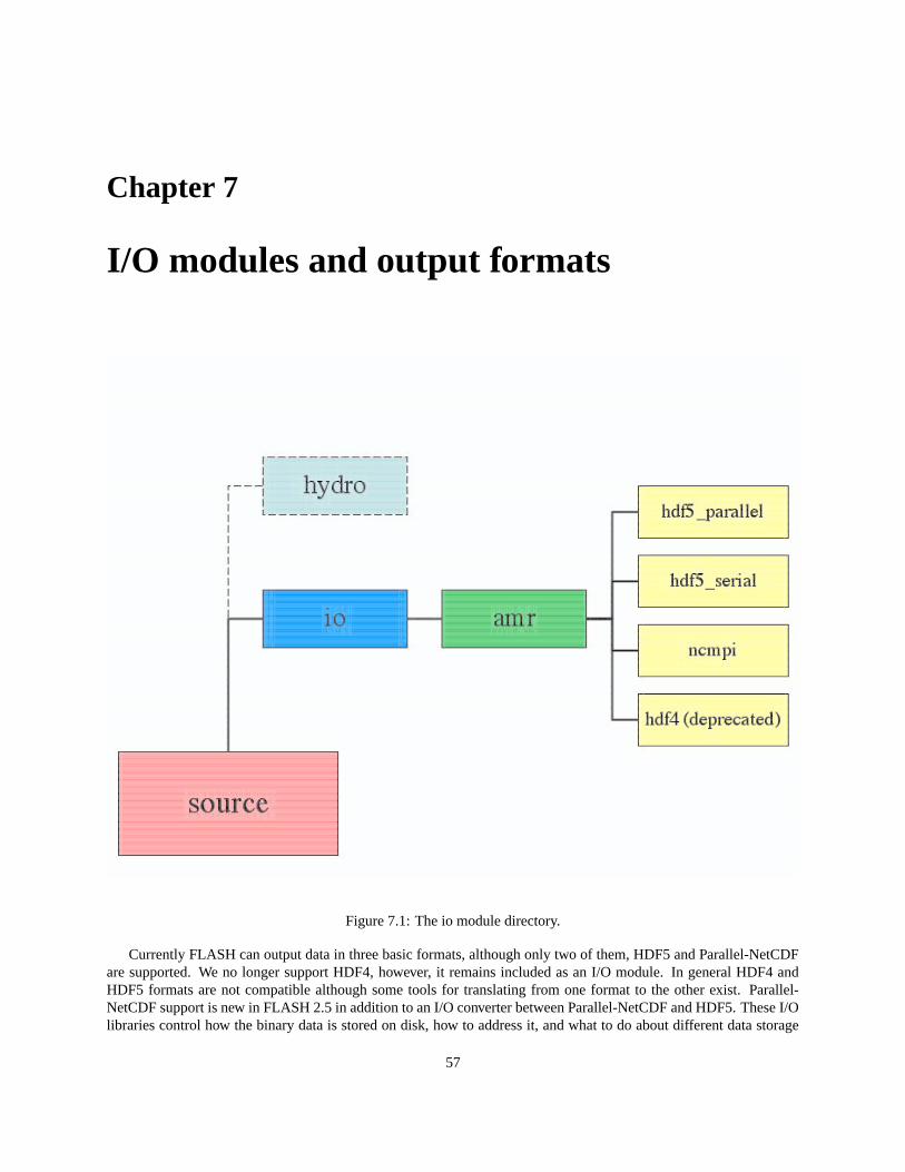
Chapter 7
I/O modules and output formats
Figure 7.1: The io module directory.
Currently FLASH can output data in three basic formats, although only two of them, HDF5 and Parallel-NetCDFare supported. We no longer support HDF4, however, it remains included as an I/O module. In general HDF4 andHDF5 formats are not compatible although some tools for translating from one format to the other exist. Parallel-NetCDF support is new in FLASH 2.5 in addition to an I/O converter between Parallel-NetCDF and HDF5. These I/Olibraries control how the binary data is stored on disk, how to address it, and what to do about different data storage
57

58 CHAPTER 7. I/O MODULES AND OUTPUT FORMATS
on different platforms. The mapping of FLASH data-structures to records in these files is controlled by the FLASHI/O modules. These file formats have different strengths and weaknesses, and the data layout is different for each filetype.
Various techniques can be used to write the data to disk. The first is to move all the data to a single processor foroutput. Secondly, each processor can write to a separate file and finally, each processor can each use parallel access towrite to a single file. In general, parallel access to a single file will provide the best performance. On some platforms,such as Linux clusters, there may not be a parallel file system, so moving all the data to a single processor is the bestsolution.
The hdf I/O modules use the HDF application programming interface (API) for organizing data in a databasefashion. In addition to the raw data, information about the data type and byte ordering (little or big endian), rank,and dimensions of the dataset is stored. This makes the HDF format extremely portable across platforms. Differentpackages can query the file for its contents without knowing the details of the routine that generated the data.
HDF4 was limited to files < 2 GB in size and furthermore, the official release did not support parallel I/O. Forthese reasons we no longer support HDF4 and instead support HDF5 which was released to address these limitations.HDF5 is supported on a large variety of platforms and offers the same functionality as HDF4, with the addition oflarge file support and parallel I/O via MPI-I/O. Information about the different versions of HDF can be found athttp://hdf.ncsa.uiuc.edu.
Parallel-NetCDF can also handle files > 2GB and is available at http://www-unix.mcs.anl.gov/parallel-netcdf/.At this time we require the latest version available 0.9.4. The PNetCDF API appears to still be expanding and the addi-tional capabilities should increase the I/O performance of FLASH in a few areas, particularly the use of MPI-Datatypesto output user defined datatypes. The motivation for releasing an alternative to HDF has been two fold. First, there hasbeen some debate over performance between HDF5 and PNetCDF which is slimmer application, more closely alignedto MPI-IO than HDF5. Our preliminary results showed PNetCDF running up to fifty percent faster than HDF5. How-ever, since PNetCDF does not yet have implementation for user defined data structures, it is not possible to fullyunderstand the performance differences between these two packages in the context of FLASH. Our second reason forreleasing PNetCDF is simply to have a portable alternative to HDF5 which had given some users problems in the past.
The following sections assume that the proper I/O packages are already installed on your machine. As of FLASH2.2, the default I/O format is HDF5; the default I/O module is hdf5_serial (see Table 7.1). The I/O modulesin FLASH have two responsibilities—generating and restarting from checkpoint files, and generating plot files. Acheckpoint file contains all the information needed to restart the simulation. The data is stored at the same precision(8-byte reals) as it is carried in the code and includes all of the variables. A plotfile contains all the information neededto interpret the tree structure maintained by FLASH and includes a user-defined subset of the variables. Furthermore,the data is stored at reduced precision to conserve space.
Table 7.1 summarizes the different modules which come with FLASH.
Table 7.1: I/O modules available in FLASH.
Module name Descriptionamr/hdf4 Hierarchical Data Format (HDF) 4 output. A single HDF file is
created by the master processor and all data are moved to thisprocessor via explicit MPI sends and receives before writing tothe file. (Deprecated)
amr/hdf5_serial Hierarchical Data Format (HDF) 5 output. Each processorpasses its data to processor 0 through explicit MPI sends andreceives. Processor 0 does all of the writing. The resulting fileformat is identical to the parallel version; the only difference ishow the data is moved during the writing.
amr/hdf5_parallel Hierarchical Data Format (HDF) 5 output. A single HDF5 fileis created, with each processor writing its data to the same filesimultaneously. This relies on the underlying MPIIO layer inHDF5.
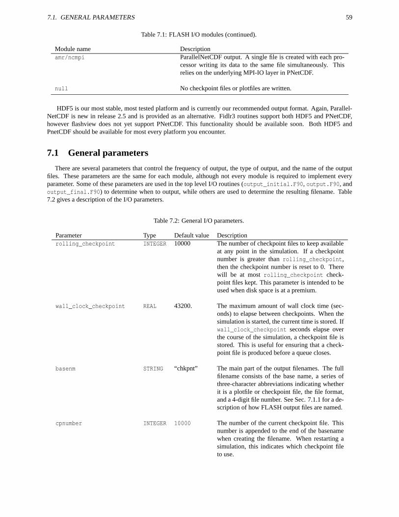
7.1. GENERAL PARAMETERS 59
Table 7.1: FLASH I/O modules (continued).
Module name Descriptionamr/ncmpi ParallelNetCDF output. A single file is created with each pro-
cessor writing its data to the same file simultaneously. Thisrelies on the underlying MPI-IO layer in PNetCDF.
null No checkpoint files or plotfiles are written.
HDF5 is our most stable, most tested platform and is currently our recommended output format. Again, Parallel-NetCDF is new in release 2.5 and is provided as an alternative. Fidlr3 routines support both HDF5 and PNetCDF,however flashview does not yet support PNetCDF. This functionality should be available soon. Both HDF5 andPnetCDF should be available for most every platform you encounter.
7.1 General parameters
There are several parameters that control the frequency of output, the type of output, and the name of the outputfiles. These parameters are the same for each module, although not every module is required to implement everyparameter. Some of these parameters are used in the top level I/O routines (output_initial.F90, output.F90, andoutput_final.F90) to determine when to output, while others are used to determine the resulting filename. Table7.2 gives a description of the I/O parameters.
Table 7.2: General I/O parameters.
Parameter Type Default value Descriptionrolling_checkpoint INTEGER 10000 The number of checkpoint files to keep available
at any point in the simulation. If a checkpointnumber is greater than rolling_checkpoint,then the checkpoint number is reset to 0. Therewill be at most rolling_checkpoint check-point files kept. This parameter is intended to beused when disk space is at a premium.
wall_clock_checkpoint REAL 43200. The maximum amount of wall clock time (sec-onds) to elapse between checkpoints. When thesimulation is started, the current time is stored. Ifwall_clock_checkpoint seconds elapse overthe course of the simulation, a checkpoint file isstored. This is useful for ensuring that a check-point file is produced before a queue closes.
basenm STRING “chkpnt” The main part of the output filenames. The fullfilename consists of the base name, a series ofthree-character abbreviations indicating whetherit is a plotfile or checkpoint file, the file format,and a 4-digit file number. See Sec. 7.1.1 for a de-scription of how FLASH output files are named.
cpnumber INTEGER 10000 The number of the current checkpoint file. Thisnumber is appended to the end of the basenamewhen creating the filename. When restarting asimulation, this indicates which checkpoint fileto use.
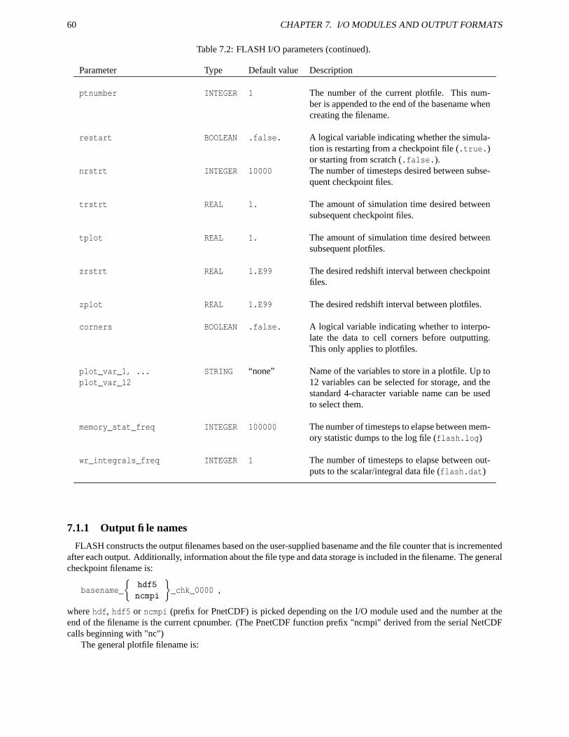
60 CHAPTER 7. I/O MODULES AND OUTPUT FORMATS
Table 7.2: FLASH I/O parameters (continued).
Parameter Type Default value Description
ptnumber INTEGER 1 The number of the current plotfile. This num-ber is appended to the end of the basename whencreating the filename.
restart BOOLEAN .false. A logical variable indicating whether the simula-tion is restarting from a checkpoint file (.true.)or starting from scratch (.false.).
nrstrt INTEGER 10000 The number of timesteps desired between subse-quent checkpoint files.
trstrt REAL 1. The amount of simulation time desired betweensubsequent checkpoint files.
tplot REAL 1. The amount of simulation time desired betweensubsequent plotfiles.
zrstrt REAL 1.E99 The desired redshift interval between checkpointfiles.
zplot REAL 1.E99 The desired redshift interval between plotfiles.
corners BOOLEAN .false. A logical variable indicating whether to interpo-late the data to cell corners before outputting.This only applies to plotfiles.
plot_var_1, ...plot_var_12
STRING “none” Name of the variables to store in a plotfile. Up to12 variables can be selected for storage, and thestandard 4-character variable name can be usedto select them.
memory_stat_freq INTEGER 100000 The number of timesteps to elapse between mem-ory statistic dumps to the log file (flash.log)
wr_integrals_freq INTEGER 1 The number of timesteps to elapse between out-puts to the scalar/integral data file (flash.dat)
7.1.1 Output file names
FLASH constructs the output filenames based on the user-supplied basename and the file counter that is incrementedafter each output. Additionally, information about the file type and data storage is included in the filename. The generalcheckpoint filename is:
basename_
hdf5
ncmpi
_chk_0000 ,
where hdf, hdf5 or ncmpi (prefix for PnetCDF) is picked depending on the I/O module used and the number at theend of the filename is the current cpnumber. (The PnetCDF function prefix "ncmpi" derived from the serial NetCDFcalls beginning with "nc")
The general plotfile filename is:
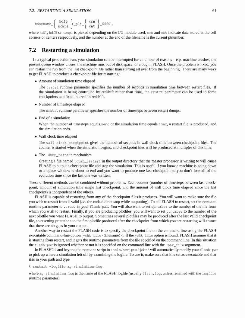
7.2. RESTARTING A SIMULATION 61
basename_
hdf5
ncmpi
_plt_
crn
cnt
_0000 ,
where hdf , hdf5 or ncmpi is picked depending on the I/O module used, crn and cnt indicate data stored at the cellcorners or centers respectively, and the number at the end of the filename is the current ptnumber.
7.2 Restarting a simulation
In a typical production run, your simulation can be interrupted for a number of reasons—e.g. machine crashes, thepresent queue window closes, the machine runs out of disk space, or a bug in FLASH. Once the problem is fixed, youcan restart the run from the last checkpoint file rather than starting all over from the beginning. There are many waysto get FLASH to produce a checkpoint file for restarting:
• Amount of simulation time elapsed
The trstrt runtime parameter specifies the number of seconds in simulation time between restart files. Ifthe simulation is being controlled by redshift rather than time, the zrstrt parameter can be used to forcecheckpoints at a fixed interval in redshift.
• Number of timesteps elapsed
The nrstrt runtime parameter specifies the number of timesteps between restart dumps.
• End of a simulation
When the number of timesteps equals nend or the simulation time equals tmax, a restart file is produced, andthe simulation ends.
• Wall clock time elapsed
The wall_clock_checkpoint gives the number of seconds in wall clock time between checkpoint files. Thecounter is started when the simulation begins, and checkpoint files will be produced at multiples of this time.
• The .dump_restart mechanism
Creating a file named .dump_restart in the output directory that the master processor is writing to will causeFLASH to output a checkpoint file and stop the simulation. This is useful if you know a machine is going downor a queue window is about to end and you want to produce one last checkpoint so you don’t lose all of theevolution time since the last one was written.
These different methods can be combined without problems. Each counter (number of timesteps between last check-point, amount of simulation time single last checkpoint, and the amount of wall clock time elapsed since the lastcheckpoint) is independent of the others.
FLASH is capable of restarting from any of the checkpoint files it produces. You will want to make sure the fileyou wish to restart from is valid (i.e. the code did not stop while outputting). To tell FLASH to restart, set the restartruntime parameter to .true. in your flash.par. You will also want to set cpnumber to the number of the file fromwhich you wish to restart. Finally, if you are producing plotfiles, you will want to set ptnumber to the number of thenext plotfile you want FLASH to output. Sometimes several plotfiles may be produced after the last valid checkpointfile, so resetting ptnumber to the first plotfile produced after the checkpoint from which you are restarting will ensurethat there are no gaps in your output.
Another way to restart the FLASH code is to specify the checkpoint file on the command line using the FLASHexecutable command-line option (-chk_file<filename>). If the -chk_file option is found, FLASH assumes that itis starting from restart, and it gets the runtime parameters from the file specified on the command line. In this situationthe flash.par is ignored whether or not it is specified on the command line with the -par_file argument.
In FLASH2.4 and beyond,the restart script in tools/scripts/jobs/will automatically modify your flash.parto pick up where a simulation left off by examining the logfile. To use it, make sure that it is set as executable and thatit is in your path and type
% restart -logfile my_simulation.log
where my_simulation.log is the name of the FLASH logfile (usually flash.log, unless renamed with the logfileruntime parameter).
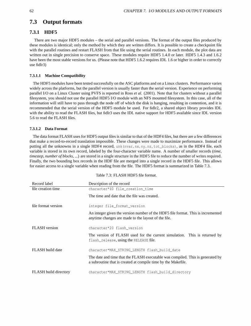
62 CHAPTER 7. I/O MODULES AND OUTPUT FORMATS
7.3 Output formats
7.3.1 HDF5
There are two major HDF5 modules – the serial and parallel versions. The format of the output files produced bythese modules is identical; only the method by which they are written differs. It is possible to create a checkpoint filewith the parallel routines and restart FLASH from that file using the serial routines. In each module, the plot data arewritten out in single precision to conserve space. These modules require HDF5 1.4.0 or later. HDF5 1.4.3 and 1.6.2have been the most stable versions for us. (Please note that HDF5 1.6.2 requires IDL 1.6 or higher in order to correctlyuse fidlr3)
7.3.1.1 Machine Compatibility
The HDF5 modules have been tested successfully on the ASC platforms and on a Linux clusters. Performance varieswidely across the platforms, but the parallel version is usually faster than the serial version. Experience on performingparallel I/O on a Linux Cluster using PVFS is reported in Ross et al. (2001). Note that for clusters without a parallelfilesystem, you should not use the parallel HDF5 I/O module with an NFS mounted filesystem. In this case, all of theinformation will still have to pass through the node off of which the disk is hanging, resulting in contention, and it isrecommended that the serial version of the HDF5 module be used. For fidlr2, a shared object library provides IDLwith the ability to read the FLASH files, but fidlr3 uses the IDL native support for HDF5 available since IDL version5.6 to read the FLASH files.
7.3.1.2 Data Format
The data format FLASH uses for HDF5 output files is similar to that of the HDF4 files, but there are a few differencesthat make a record-to-record translation impossible. These changes were made to maximize performance. Instead ofputting all the unknowns in a single HDF4 record, unk(nvar,nx,ny,nz,tot_blocks), as in the HDF4 file, eachvariable is stored in its own record, labeled by the four-character variable name. A number of smaller records (time,timestep, number of blocks, ...) are stored in a single structure in the HDF5 file to reduce the number of writes required.Finally, the two bounding box records in the HDF file are merged into a single record in the HDF5 file. This allowsfor easier access to a single variable when reading from the file. The HDF5 format is summarized in Table 7.3.
Table 7.3: FLASH HDF5 file format.
Record label Description of the recordfile creation time character*40 file_creation_time
The time and date that the file was created.
file format version integer file_format_version
An integer given the version number of the HDF5 file format. This is incrementedanytime changes are made to the layout of the file.
FLASH version character*20 flash_version
The version of FLASH used for the current simulation. This is returned byflash_release, using the RELEASE file.
FLASH build date character*MAX_STRING_LENGTH flash_build_date
The date and time that the FLASH executable was compiled. This is generated bya subroutine that is created at compile time by the Makefile.
FLASH build directory character*MAX_STRING_LENGTH flash_build_directory
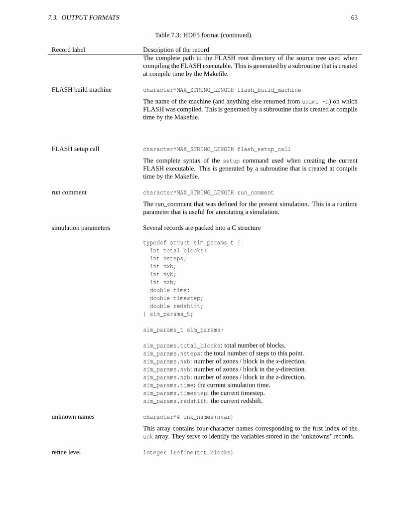
7.3. OUTPUT FORMATS 63
Table 7.3: HDF5 format (continued).
Record label Description of the recordThe complete path to the FLASH root directory of the source tree used whencompiling the FLASH executable. This is generated by a subroutine that is createdat compile time by the Makefile.
FLASH build machine character*MAX_STRING_LENGTH flash_build_machine
The name of the machine (and anything else returned from uname -a) on whichFLASH was compiled. This is generated by a subroutine that is created at compiletime by the Makefile.
FLASH setup call character*MAX_STRING_LENGTH flash_setup_call
The complete syntax of the setup command used when creating the currentFLASH executable. This is generated by a subroutine that is created at compiletime by the Makefile.
run comment character*MAX_STRING_LENGTH run_comment
The run_comment that was defined for the present simulation. This is a runtimeparameter that is useful for annotating a simulation.
simulation parameters Several records are packed into a C structure
typedef struct sim_params_t int total_blocks;int nsteps;int nxb;int nyb;int nzb;double time;double timestep;double redshift;
sim_params_t;
sim_params_t sim_params;
sim_params.total_blocks: total number of blocks.sim_params.nsteps: the total number of steps to this point.sim_params.nxb: number of zones / block in the x-direction.sim_params.nyb: number of zones / block in the y-direction.sim_params.nzb: number of zones / block in the z-direction.sim_params.time: the current simulation time.sim_params.timestep: the current timestep.sim_params.redshift: the current redshift.
unknown names character*4 unk_names(nvar)
This array contains four-character names corresponding to the first index of theunk array. They serve to identify the variables stored in the ‘unknowns’ records.
refine level integer lrefine(tot_blocks)
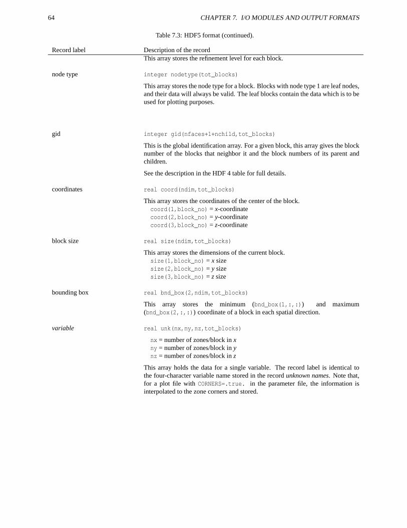
64 CHAPTER 7. I/O MODULES AND OUTPUT FORMATS
Table 7.3: HDF5 format (continued).
Record label Description of the recordThis array stores the refinement level for each block.
node type integer nodetype(tot_blocks)
This array stores the node type for a block. Blocks with node type 1 are leaf nodes,and their data will always be valid. The leaf blocks contain the data which is to beused for plotting purposes.
gid integer gid(nfaces+1+nchild,tot_blocks)
This is the global identification array. For a given block, this array gives the blocknumber of the blocks that neighbor it and the block numbers of its parent andchildren.
See the description in the HDF 4 table for full details.
coordinates real coord(ndim,tot_blocks)
This array stores the coordinates of the center of the block.coord(1,block_no) = x-coordinatecoord(2,block_no) = y-coordinatecoord(3,block_no) = z-coordinate
block size real size(ndim,tot_blocks)
This array stores the dimensions of the current block.size(1,block_no) = x sizesize(2,block_no) = y sizesize(3,block_no) = z size
bounding box real bnd_box(2,ndim,tot_blocks)
This array stores the minimum (bnd_box(1,:,:)) and maximum(bnd_box(2,:,:)) coordinate of a block in each spatial direction.
variable real unk(nx,ny,nz,tot_blocks)
nx = number of zones/block in xny = number of zones/block in ynz = number of zones/block in z
This array holds the data for a single variable. The record label is identical tothe four-character variable name stored in the record unknown names. Note that,for a plot file with CORNERS=.true. in the parameter file, the information isinterpolated to the zone corners and stored.
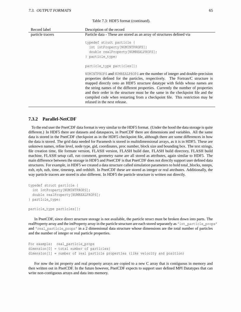
7.3. OUTPUT FORMATS 65
Table 7.3: HDF5 format (continued).
Record label Description of the recordparticle tracers Particle data - These are stored as an array of structures defined via
typedef struct particle int intProperty[NUMINTPROPS];double realProperty[NUMREALPROPS];
particle_type;
particle_type particles[];
NUMINTPROPS and NUMREALPROPS are the number of integer and double-precisionproperties defined for the particles, respectively. The Fortran/C structure ismapped directly onto an HDF5 structure datatype with fields whose names arethe string names of the different properties. Currently the number of propertiesand their order in the structure must be the same in the checkpoint file and thecompiled code when restarting from a checkpoint file. This restriction may berelaxed in the next release.
7.3.2 Parallel-NetCDF
To the end user the PnetCDF data format is very similar to the HDF5 format. (Under the hood the data storage is quitedifferent.) In HDF5 there are datasets and dataspaces, in PnetCDF there are dimensions and variables. All the samedata is stored in the PnetCDF checkpoint as in the HDF5 checkpoint file, although there are some differences in howthe data is stored. The grid data needed for Paramesh is stored in multidimensional arrays, as it is in HDF5. These areunknown names, refine level, node type, gid, coordinates, proc number, block size and bounding box. The text strings,file creation time, file formate version, FLASH version, FLASH build date, FLASH build directory, FLASH buildmachine, FLASH setup call, run comment, geometry name are all stored as attributes, again similar to HDF5. Themain difference between the storage in HDF5 and PnetCDF is that PnetCDF does not directly support user defined datastructures. For example, in HDF5 we created a data structure called simulation parameters to hold total_blocks, nsteps,nxb, nyb, nzb, time, timestep, and redshift. In PnetCDF these are stored as integer or real attributes. Additionally, theway particle tracers are stored is also different. In HDF5 the particle structure is written out directly.
typedef struct particle int intProperty[NUMINTPROPS];double realProperty[NUMREALPROPS];
particle_type;
particle_type particles[];
In PnetCDF, since direct structure storage is not available, the particle struct must be broken down into parts. TherealProperty array and the intProperty array in the particle structure are each stored separately as "int_particle_props"and "real_particle_props" in a 2 dimensional data structure whose dimensions are the total number of particlesand the number of integer or real particle properties.
For example: real_particle_propsdimension[0] = total number of particlesdimension[1] = number of real particle properties (like velocity and position)
For now the int property and real property arrays are copied to a new C array that is contiguous in memory andthen written out in PnetCDF. In the future however, PnetCDF expects to support user defined MPI Datatypes that canwrite non-contiguous arrays and data into memory.
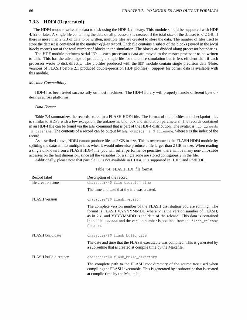
66 CHAPTER 7. I/O MODULES AND OUTPUT FORMATS
7.3.3 HDF4 (Deprecated)
The HDF4 module writes the data to disk using the HDF 4.x library. This module should be supported with HDF4.1r2 or later. A single file containing the data on all processors is created, if the total size of the dataset is < 2 GB. Ifthere is more than 2 GB of data to be written, multiple files are created to store the data. The number of files used tostore the dataset is contained in the number of files record. Each file contains a subset of the blocks (stored in the localblocks record) out of the total number of blocks in the simulation. The blocks are divided along processor boundaries.
The HDF module performs serial I/O — each processor’s data are moved to the master processor to be writtento disk. This has the advantage of producing a single file for the entire simulation but is less efficient than if eachprocessor wrote to disk directly. The plotfiles produced with the HDF module contain single precision data (Note:versions of FLASH before 2.1 produced double-precision HDF plotfiles). Support for corner data is available withthis module.
Machine Compatibility
HDF4 has been tested successfully on most machines. The HDF4 library will properly handle different byte or-derings across platforms.
Data Format
Table 7.4 summarizes the records stored in a FLASH HDF4 file. The format of the plotfiles and checkpoint filesis similar to HDF5 with a few exception, the unknowns, bnd_box and simulation parameters. The records containedin an HDF4 file can be found via the hdp command that is part of the HDF4 distribution. The syntax is hdp dumpsds-h filename. The contents of a record can be output by hdp dumpsds -i N filename, where N is the index of therecord.
As described above, HDF4 cannot produce files > 2 GB in size. This is overcome in the FLASH HDF4 module bysplitting the dataset into multiple files when it would otherwise produce a file larger than 2 GB in size. When readinga single unknown from a FLASH HDF4 file, you will suffer performance penalties; there will be many non-unit-strideaccesses on the first dimension, since all the variables for a single zone are stored contiguously in the file.
Additionally, please note that particle IO is not available in HDF4. It is supported in HDF5 and PnetCDF.
Table 7.4: FLASH HDF file format.
Record label Description of the recordfile creation time character*40 file_creation_time
The time and date that the file was created.
FLASH version character*20 flash_version
The complete version number of the FLASH distribution you are running. Theformat is FLASH V.YYYYMMDD where V is the version number of FLASH,as in 2.x, and YYYYMMDD is the date of the release. This data is containedin the file RELEASE and the version number is obtained from the flash_releasefunction.
FLASH build date character*80 flash_build_date
The date and time that the FLASH executable was compiled. This is generated bya subroutine that is created at compile time by the Makefile.
FLASH build directory character*80 flash_build_directory
The complete path to the FLASH root directory of the source tree used whencompiling the FLASH executable. This is generated by a subroutine that is createdat compile time by the Makefile.
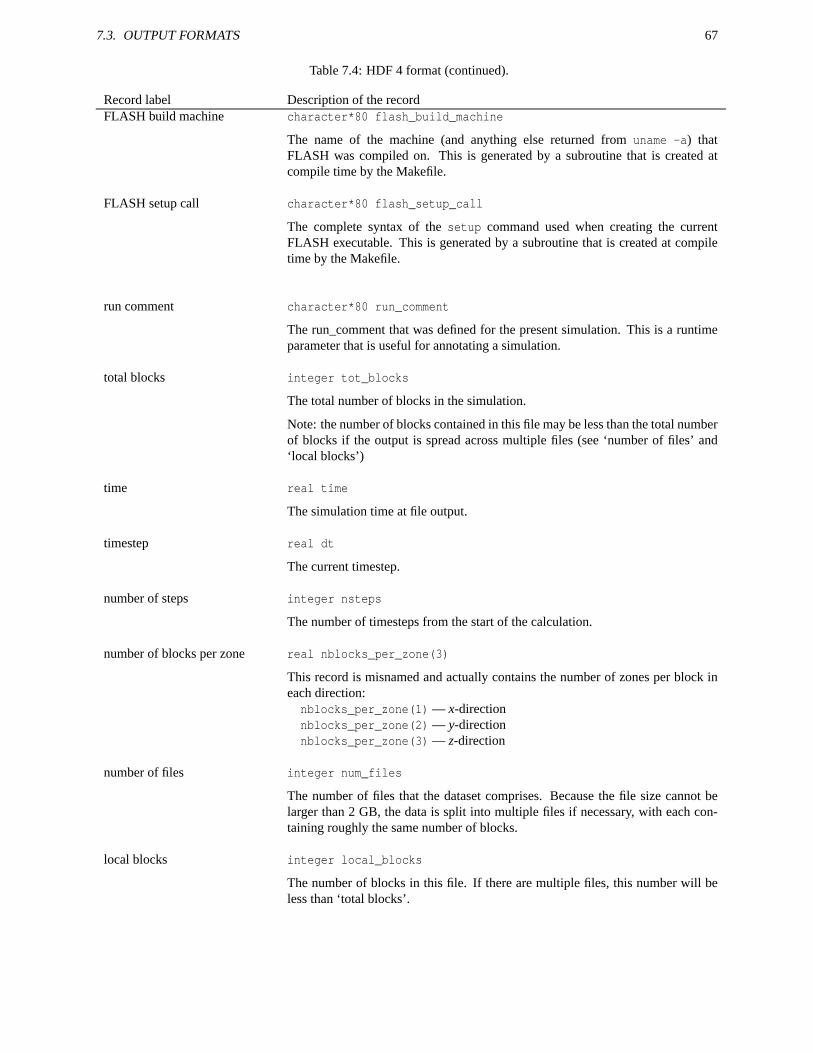
7.3. OUTPUT FORMATS 67
Table 7.4: HDF 4 format (continued).
Record label Description of the recordFLASH build machine character*80 flash_build_machine
The name of the machine (and anything else returned from uname -a) thatFLASH was compiled on. This is generated by a subroutine that is created atcompile time by the Makefile.
FLASH setup call character*80 flash_setup_call
The complete syntax of the setup command used when creating the currentFLASH executable. This is generated by a subroutine that is created at compiletime by the Makefile.
run comment character*80 run_comment
The run_comment that was defined for the present simulation. This is a runtimeparameter that is useful for annotating a simulation.
total blocks integer tot_blocks
The total number of blocks in the simulation.
Note: the number of blocks contained in this file may be less than the total numberof blocks if the output is spread across multiple files (see ‘number of files’ and‘local blocks’)
time real time
The simulation time at file output.
timestep real dt
The current timestep.
number of steps integer nsteps
The number of timesteps from the start of the calculation.
number of blocks per zone real nblocks_per_zone(3)
This record is misnamed and actually contains the number of zones per block ineach direction:nblocks_per_zone(1) — x-directionnblocks_per_zone(2) — y-directionnblocks_per_zone(3) — z-direction
number of files integer num_files
The number of files that the dataset comprises. Because the file size cannot belarger than 2 GB, the data is split into multiple files if necessary, with each con-taining roughly the same number of blocks.
local blocks integer local_blocks
The number of blocks in this file. If there are multiple files, this number will beless than ‘total blocks’.
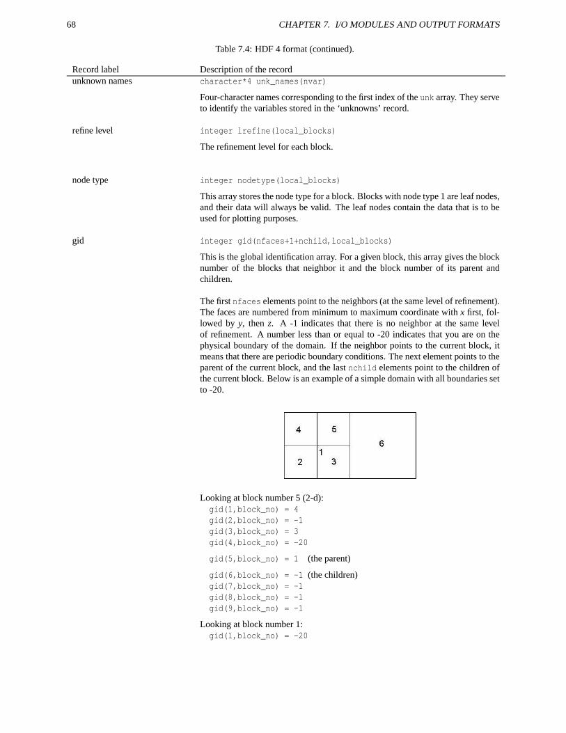
68 CHAPTER 7. I/O MODULES AND OUTPUT FORMATS
Table 7.4: HDF 4 format (continued).
Record label Description of the recordunknown names character*4 unk_names(nvar)
Four-character names corresponding to the first index of the unk array. They serveto identify the variables stored in the ‘unknowns’ record.
refine level integer lrefine(local_blocks)
The refinement level for each block.
node type integer nodetype(local_blocks)
This array stores the node type for a block. Blocks with node type 1 are leaf nodes,and their data will always be valid. The leaf nodes contain the data that is to beused for plotting purposes.
gid integer gid(nfaces+1+nchild,local_blocks)
This is the global identification array. For a given block, this array gives the blocknumber of the blocks that neighbor it and the block number of its parent andchildren.
The first nfaces elements point to the neighbors (at the same level of refinement).The faces are numbered from minimum to maximum coordinate with x first, fol-lowed by y, then z. A -1 indicates that there is no neighbor at the same levelof refinement. A number less than or equal to -20 indicates that you are on thephysical boundary of the domain. If the neighbor points to the current block, itmeans that there are periodic boundary conditions. The next element points to theparent of the current block, and the last nchild elements point to the children ofthe current block. Below is an example of a simple domain with all boundaries setto -20.
Looking at block number 5 (2-d):gid(1,block_no) = 4gid(2,block_no) = -1gid(3,block_no) = 3gid(4,block_no) = -20
gid(5,block_no) = 1 (the parent)
gid(6,block_no) = -1 (the children)gid(7,block_no) = -1gid(8,block_no) = -1gid(9,block_no) = -1
Looking at block number 1:gid(1,block_no) = -20
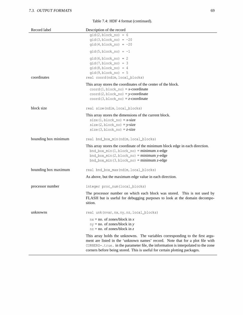
7.3. OUTPUT FORMATS 69
Table 7.4: HDF 4 format (continued).
Record label Description of the recordgid(2,block_no) = 6gid(3,block_no) = -20gid(4,block_no) = -20
gid(5,block_no) = -1
gid(6,block_no) = 2gid(7,block_no) = 3gid(8,block_no) = 4gid(9,block_no) = 5
coordinates real coord(ndim,local_blocks)
This array stores the coordinates of the center of the block.coord(1,block_no) = x-coordinatecoord(2,block_no) = y-coordinatecoord(3,block_no) = z-coordinate
block size real size(ndim,local_blocks)
This array stores the dimensions of the current block.size(1,block_no) = x-sizesize(2,block_no) = y-sizesize(3,block_no) = z-size
bounding box minimum real bnd_box_min(ndim,local_blocks)
This array stores the coordinate of the minimum block edge in each direction.bnd_box_min(1,block_no) = minimum x-edgebnd_box_min(2,block_no) = minimum y-edgebnd_box_min(3,block_no) = minimum z-edge
bounding box maximum real bnd_box_max(ndim,local_blocks)
As above, but the maximum edge value in each direction.
processor number integer proc_num(local_blocks)
The processor number on which each block was stored. This is not used byFLASH but is useful for debugging purposes to look at the domain decompo-sition.
unknowns real unk(nvar,nx,ny,nz,local_blocks)
nx = no. of zones/block in xny = no. of zones/block in ynz = no. of zones/block in z
This array holds the unknowns. The variables corresponding to the first argu-ment are listed in the ‘unknown names’ record. Note that for a plot file withCORNERS=.true. in the parameter file, the information is interpolated to the zonecorners before being stored. This is useful for certain plotting packages.
70 CHAPTER 7. I/O MODULES AND OUTPUT FORMATS
7.4 IO Converter
This tool, new in FLASH 2.5 allows a user to convert an I/O file from HDF5 to PNetCDF or from PNetCDF toHDF5. This is done primarily through the command line setup with the option -io_convert=from:to where fromand to are the entire paths.
For example, to convert a checkpoint file from a sedov run:setup sedov -2d -io_convert=io/amr/hdf5_parallel:io/amr/ncmpi
Besides this change, FLASH will run as usual. This tool can be used to simply convert a file or to restart a run withone I/O module and continue it with another. In order to run the converter there must be a flash.par file with restartset to true and a valid I/O checkpoint file. Without the I/O converter running the code with restart = .true. , a givencheckpoint file, hdf5_chk_0005 is read in and the next output is hdf5_chk_0006. When the "io_convert" option is usedat setup time the initial checkpoint file is translated into its new format and then the code will continue as usual. Forexample, hdf5_chk_0005 is read in, the next output file is ncmpi_chk_0005, and next is ncmpi_chk_0006.
7.5 Working with output files
The checkpoint file output formats offer great flexibility when visualizing the data. The visualization program doesnot have to know the details of how the file was written; rather it can query the file to find the number of dimensions,block sizes, variable data etc that it needs to visualize the data. IDL routines for reading HDF, HDF5 and PnetCDFformats are provided in tools/fidlr3/. These can be used interactively though the IDL command line (see Sec. 5).
7.6 User-defined variables
user_var is called just before output files are written. This routine allows the calculation of user-defined variables,which can then be written out for plotting or analysis. These user-defined variables must be defined in the FLASHcode (see Configuration layer, Chapter 5).
The supplied user_var, in source/io/user_var.F90, looks for two variables, vrtz and cond— the z-componentof vorticity, and a (thermal) conductivity. If either of these are present, the values are calculated and stored in theFLASH data structures. If the output file to be written is a checkpoint file, then both of these files are written out todisk. If the output file is a plot file, these variables will be written if the plot_var variables are set accordingly (seethe beginning of this chapter.) The supplied user_var can be used as a template for calculating other user-definedvalues. The cond variable is supplied as a convenience; it could fairly easily be calculated in a post-processing step.However, calculating vrtz would be more complicated, as its calculation requires a numerical derivative, meaningthat guard cell information (not stored in the FLASH file structures) is required. Note that these variables are stored inthe FLASH data structures and thus require memory, even though they are not used for computation.
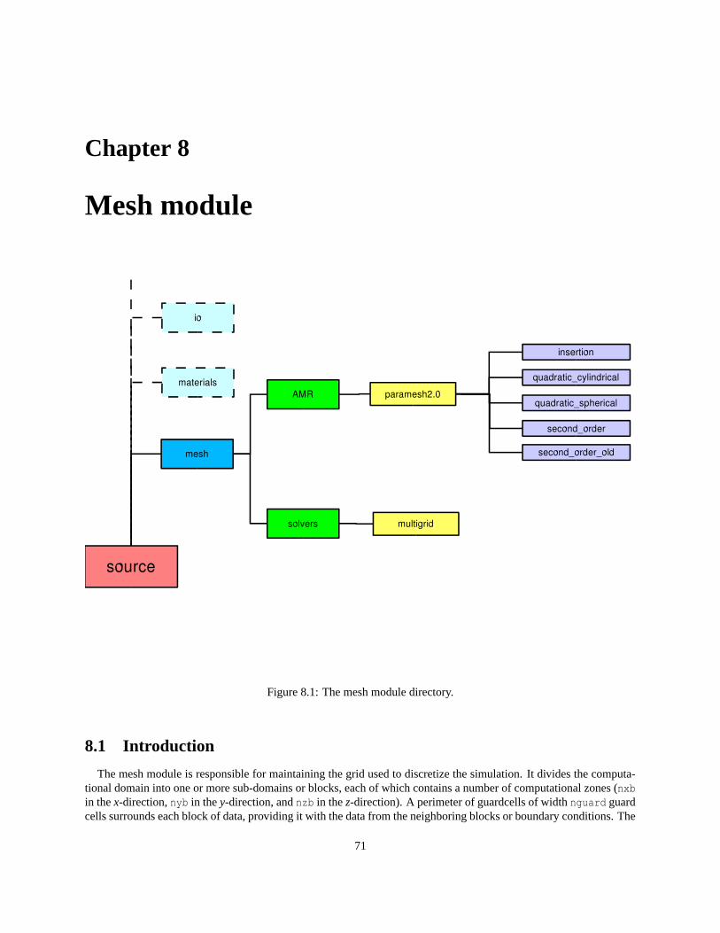
Chapter 8
Mesh module
Figure 8.1: The mesh module directory.
8.1 Introduction
The mesh module is responsible for maintaining the grid used to discretize the simulation. It divides the computa-tional domain into one or more sub-domains or blocks, each of which contains a number of computational zones (nxbin the x-direction, nyb in the y-direction, and nzb in the z-direction). A perimeter of guardcells of width nguard guardcells surrounds each block of data, providing it with the data from the neighboring blocks or boundary conditions. The
71
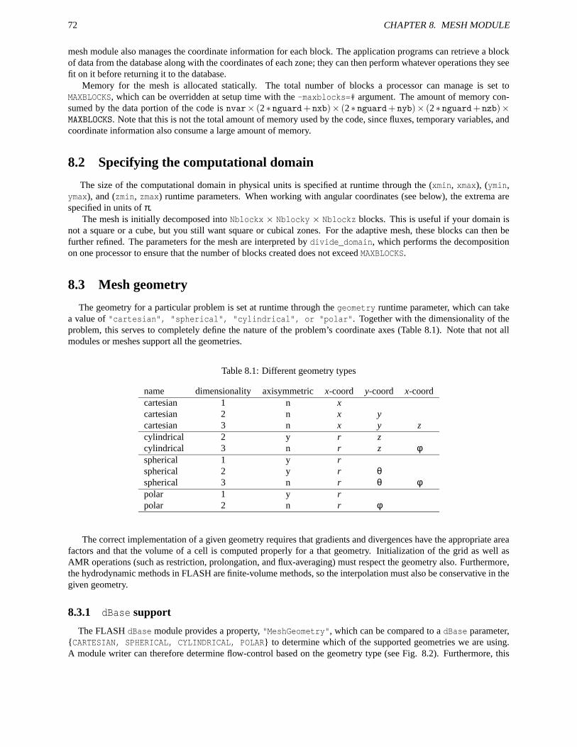
72 CHAPTER 8. MESH MODULE
mesh module also manages the coordinate information for each block. The application programs can retrieve a blockof data from the database along with the coordinates of each zone; they can then perform whatever operations they seefit on it before returning it to the database.
Memory for the mesh is allocated statically. The total number of blocks a processor can manage is set toMAXBLOCKS, which can be overridden at setup time with the -maxblocks=# argument. The amount of memory con-sumed by the data portion of the code is nvar× (2 ∗ nguard+ nxb)× (2 ∗ nguard+ nyb)× (2 ∗ nguard+ nzb)×MAXBLOCKS. Note that this is not the total amount of memory used by the code, since fluxes, temporary variables, andcoordinate information also consume a large amount of memory.
8.2 Specifying the computational domain
The size of the computational domain in physical units is specified at runtime through the (xmin, xmax), (ymin,ymax), and (zmin, zmax) runtime parameters. When working with angular coordinates (see below), the extrema arespecified in units of π.
The mesh is initially decomposed into Nblockx × Nblocky × Nblockz blocks. This is useful if your domain isnot a square or a cube, but you still want square or cubical zones. For the adaptive mesh, these blocks can then befurther refined. The parameters for the mesh are interpreted by divide_domain, which performs the decompositionon one processor to ensure that the number of blocks created does not exceed MAXBLOCKS.
8.3 Mesh geometry
The geometry for a particular problem is set at runtime through the geometry runtime parameter, which can takea value of "cartesian", "spherical", "cylindrical", or "polar". Together with the dimensionality of theproblem, this serves to completely define the nature of the problem’s coordinate axes (Table 8.1). Note that not allmodules or meshes support all the geometries.
Table 8.1: Different geometry types
name dimensionality axisymmetric x-coord y-coord x-coordcartesian 1 n xcartesian 2 n x ycartesian 3 n x y zcylindrical 2 y r zcylindrical 3 n r z φspherical 1 y rspherical 2 y r θspherical 3 n r θ φpolar 1 y rpolar 2 n r φ
The correct implementation of a given geometry requires that gradients and divergences have the appropriate areafactors and that the volume of a cell is computed properly for a that geometry. Initialization of the grid as well asAMR operations (such as restriction, prolongation, and flux-averaging) must respect the geometry also. Furthermore,the hydrodynamic methods in FLASH are finite-volume methods, so the interpolation must also be conservative in thegiven geometry.
8.3.1 dBase support
The FLASH dBase module provides a property, "MeshGeometry", which can be compared to a dBase parameter,CARTESIAN, SPHERICAL, CYLINDRICAL, POLAR to determine which of the supported geometries we are using.A module writer can therefore determine flow-control based on the geometry type (see Fig. 8.2). Furthermore, this
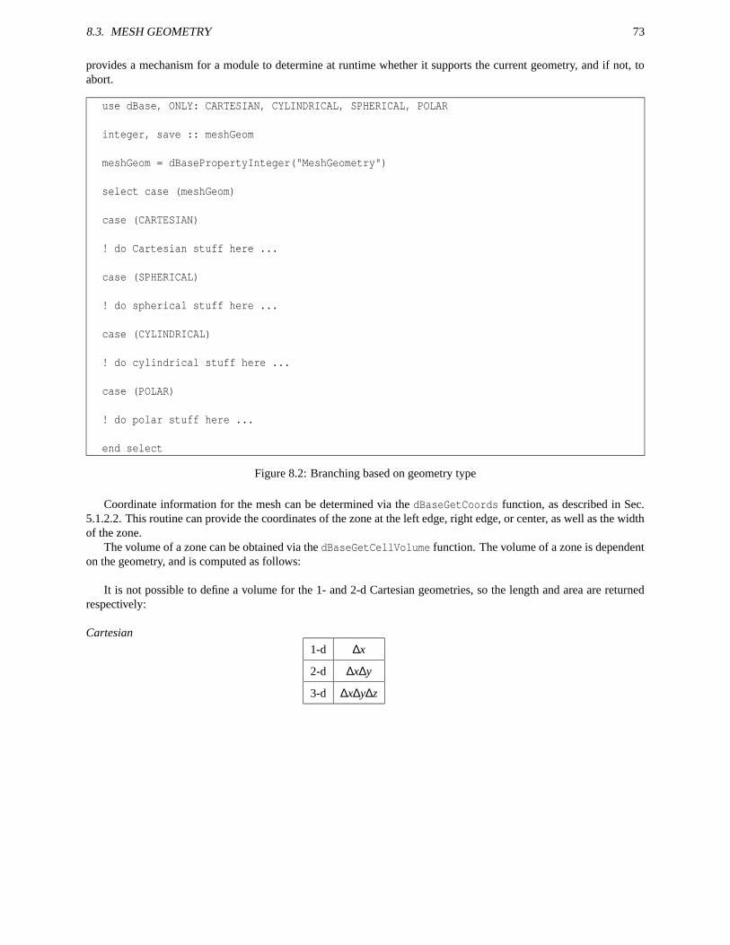
8.3. MESH GEOMETRY 73
provides a mechanism for a module to determine at runtime whether it supports the current geometry, and if not, toabort.
use dBase, ONLY: CARTESIAN, CYLINDRICAL, SPHERICAL, POLAR
integer, save :: meshGeom
meshGeom = dBasePropertyInteger("MeshGeometry")
select case (meshGeom)
case (CARTESIAN)
! do Cartesian stuff here ...
case (SPHERICAL)
! do spherical stuff here ...
case (CYLINDRICAL)
! do cylindrical stuff here ...
case (POLAR)
! do polar stuff here ...
end select
Figure 8.2: Branching based on geometry type
Coordinate information for the mesh can be determined via the dBaseGetCoords function, as described in Sec.5.1.2.2. This routine can provide the coordinates of the zone at the left edge, right edge, or center, as well as the widthof the zone.
The volume of a zone can be obtained via the dBaseGetCellVolume function. The volume of a zone is dependenton the geometry, and is computed as follows:
It is not possible to define a volume for the 1- and 2-d Cartesian geometries, so the length and area are returnedrespectively:
Cartesian
1-d ∆x
2-d ∆x∆y
3-d ∆x∆y∆z
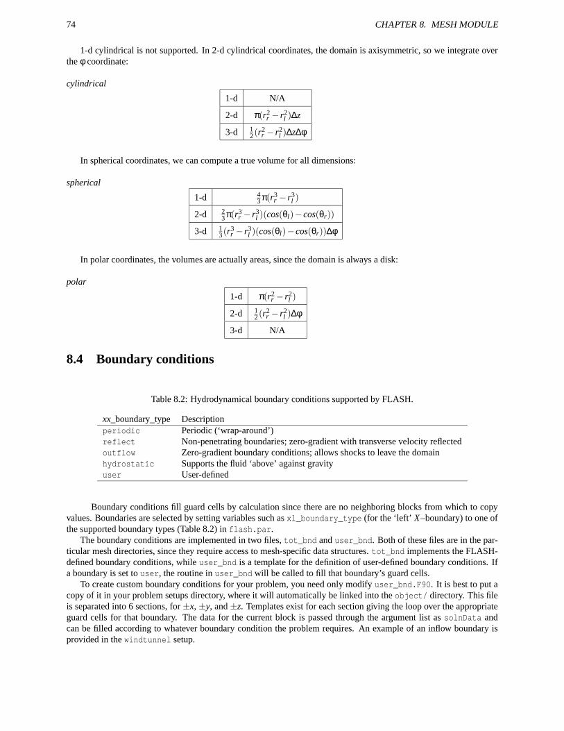
74 CHAPTER 8. MESH MODULE
1-d cylindrical is not supported. In 2-d cylindrical coordinates, the domain is axisymmetric, so we integrate overthe φ coordinate:
cylindrical
1-d N/A
2-d π(r2r − r2
l )∆z
3-d 12 (r2
r − r2l )∆z∆φ
In spherical coordinates, we can compute a true volume for all dimensions:
spherical
1-d 43 π(r3
r − r3l )
2-d 23 π(r3
r − r3l )(cos(θl)− cos(θr))
3-d 13 (r3
r − r3l )(cos(θl)− cos(θr))∆φ
In polar coordinates, the volumes are actually areas, since the domain is always a disk:
polar
1-d π(r2r − r2
l )
2-d 12 (r2
r − r2l )∆φ
3-d N/A
8.4 Boundary conditions
Table 8.2: Hydrodynamical boundary conditions supported by FLASH.
xx_boundary_type Descriptionperiodic Periodic (‘wrap-around’)reflect Non-penetrating boundaries; zero-gradient with transverse velocity reflectedoutflow Zero-gradient boundary conditions; allows shocks to leave the domainhydrostatic Supports the fluid ‘above’ against gravityuser User-defined
Boundary conditions fill guard cells by calculation since there are no neighboring blocks from which to copyvalues. Boundaries are selected by setting variables such as xl_boundary_type (for the ‘left’ X–boundary) to one ofthe supported boundary types (Table 8.2) in flash.par.
The boundary conditions are implemented in two files, tot_bnd and user_bnd. Both of these files are in the par-ticular mesh directories, since they require access to mesh-specific data structures. tot_bnd implements the FLASH-defined boundary conditions, while user_bnd is a template for the definition of user-defined boundary conditions. Ifa boundary is set to user, the routine in user_bnd will be called to fill that boundary’s guard cells.
To create custom boundary conditions for your problem, you need only modify user_bnd.F90. It is best to put acopy of it in your problem setups directory, where it will automatically be linked into the object/ directory. This fileis separated into 6 sections, for ±x, ±y, and ±z. Templates exist for each section giving the loop over the appropriateguard cells for that boundary. The data for the current block is passed through the argument list as solnData andcan be filled according to whatever boundary condition the problem requires. An example of an inflow boundary isprovided in the windtunnel setup.
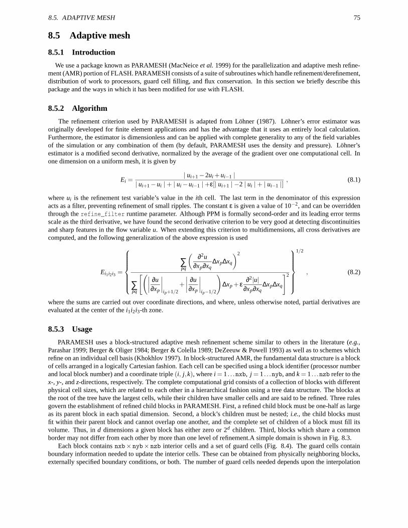
8.5. ADAPTIVE MESH 75
8.5 Adaptive mesh
8.5.1 Introduction
We use a package known as PARAMESH (MacNeice et al. 1999) for the parallelization and adaptive mesh refine-ment (AMR) portion of FLASH. PARAMESH consists of a suite of subroutines which handle refinement/derefinement,distribution of work to processors, guard cell filling, and flux conservation. In this section we briefly describe thispackage and the ways in which it has been modified for use with FLASH.
8.5.2 Algorithm
The refinement criterion used by PARAMESH is adapted from Löhner (1987). Löhner’s error estimator wasoriginally developed for finite element applications and has the advantage that it uses an entirely local calculation.Furthermore, the estimator is dimensionless and can be applied with complete generality to any of the field variablesof the simulation or any combination of them (by default, PARAMESH uses the density and pressure). Löhner’sestimator is a modified second derivative, normalized by the average of the gradient over one computational cell. Inone dimension on a uniform mesh, it is given by
Ei =| ui+1−2ui +ui−1 |
| ui+1−ui |+ | ui−ui−1 |+ε[| ui+1 | −2 | ui |+ | ui−1 |], (8.1)
where ui is the refinement test variable’s value in the ith cell. The last term in the denominator of this expressionacts as a filter, preventing refinement of small ripples. The constant ε is given a value of 10−2, and can be overriddenthrough the refine_filter runtime parameter. Although PPM is formally second-order and its leading error termsscale as the third derivative, we have found the second derivative criterion to be very good at detecting discontinuitiesand sharp features in the flow variable u. When extending this criterion to multidimensions, all cross derivatives arecomputed, and the following generalization of the above expression is used
Ei1i2i3 =
∑pq
(
∂2u∂xp∂xq
∆xp∆xq
)2
∑pq
[(
∣
∣
∣
∣
∂u∂xp
∣
∣
∣
∣
ip+1/2+
∣
∣
∣
∣
∂u∂xp
∣
∣
∣
∣
ip−1/2
)
∆xp + ε∂2|u|
∂xp∂xq∆xp∆xq
]2
1/2
, (8.2)
where the sums are carried out over coordinate directions, and where, unless otherwise noted, partial derivatives areevaluated at the center of the i1i2i3-th zone.
8.5.3 Usage
PARAMESH uses a block-structured adaptive mesh refinement scheme similar to others in the literature (e.g.,Parashar 1999; Berger & Oliger 1984; Berger & Colella 1989; DeZeeuw & Powell 1993) as well as to schemes whichrefine on an individual cell basis (Khokhlov 1997). In block-structured AMR, the fundamental data structure is a blockof cells arranged in a logically Cartesian fashion. Each cell can be specified using a block identifier (processor numberand local block number) and a coordinate triple (i, j,k), where i = 1 . . .nxb, j = 1 . . .nyb, and k = 1 . . .nzb refer to thex-, y-, and z-directions, respectively. The complete computational grid consists of a collection of blocks with differentphysical cell sizes, which are related to each other in a hierarchical fashion using a tree data structure. The blocks atthe root of the tree have the largest cells, while their children have smaller cells and are said to be refined. Three rulesgovern the establishment of refined child blocks in PARAMESH. First, a refined child block must be one-half as largeas its parent block in each spatial dimension. Second, a block’s children must be nested; i.e., the child blocks mustfit within their parent block and cannot overlap one another, and the complete set of children of a block must fill itsvolume. Thus, in d dimensions a given block has either zero or 2d children. Third, blocks which share a commonborder may not differ from each other by more than one level of refinement.A simple domain is shown in Fig. 8.3.
Each block contains nxb× nyb× nzb interior cells and a set of guard cells (Fig. 8.4). The guard cells containboundary information needed to update the interior cells. These can be obtained from physically neighboring blocks,externally specified boundary conditions, or both. The number of guard cells needed depends upon the interpolation
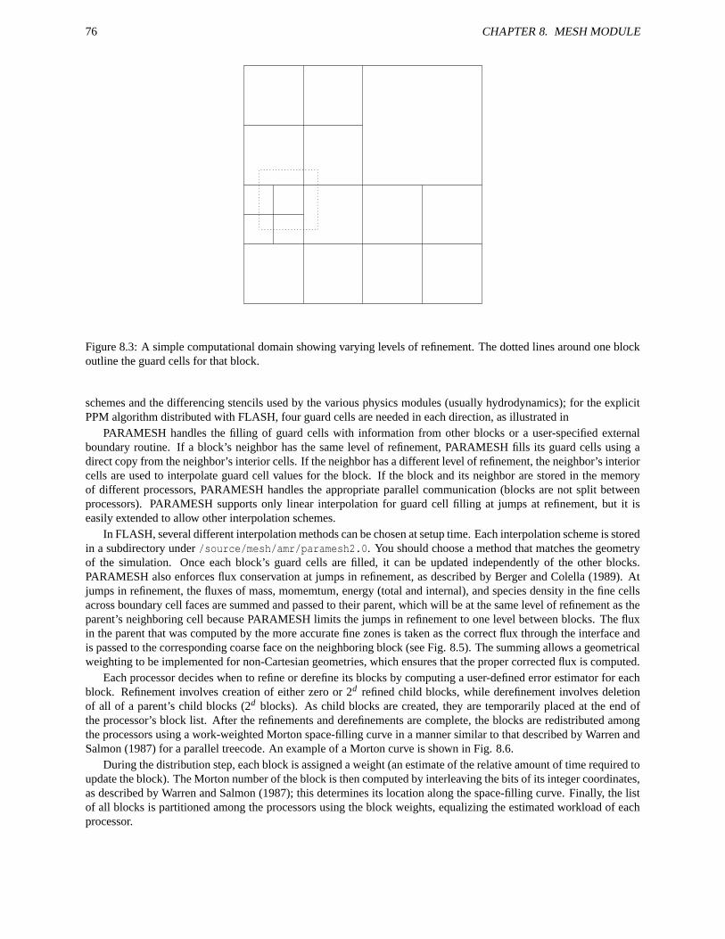
76 CHAPTER 8. MESH MODULE
Figure 8.3: A simple computational domain showing varying levels of refinement. The dotted lines around one blockoutline the guard cells for that block.
schemes and the differencing stencils used by the various physics modules (usually hydrodynamics); for the explicitPPM algorithm distributed with FLASH, four guard cells are needed in each direction, as illustrated in
PARAMESH handles the filling of guard cells with information from other blocks or a user-specified externalboundary routine. If a block’s neighbor has the same level of refinement, PARAMESH fills its guard cells using adirect copy from the neighbor’s interior cells. If the neighbor has a different level of refinement, the neighbor’s interiorcells are used to interpolate guard cell values for the block. If the block and its neighbor are stored in the memoryof different processors, PARAMESH handles the appropriate parallel communication (blocks are not split betweenprocessors). PARAMESH supports only linear interpolation for guard cell filling at jumps at refinement, but it iseasily extended to allow other interpolation schemes.
In FLASH, several different interpolation methods can be chosen at setup time. Each interpolation scheme is storedin a subdirectory under /source/mesh/amr/paramesh2.0. You should choose a method that matches the geometryof the simulation. Once each block’s guard cells are filled, it can be updated independently of the other blocks.PARAMESH also enforces flux conservation at jumps in refinement, as described by Berger and Colella (1989). Atjumps in refinement, the fluxes of mass, momemtum, energy (total and internal), and species density in the fine cellsacross boundary cell faces are summed and passed to their parent, which will be at the same level of refinement as theparent’s neighboring cell because PARAMESH limits the jumps in refinement to one level between blocks. The fluxin the parent that was computed by the more accurate fine zones is taken as the correct flux through the interface andis passed to the corresponding coarse face on the neighboring block (see Fig. 8.5). The summing allows a geometricalweighting to be implemented for non-Cartesian geometries, which ensures that the proper corrected flux is computed.
Each processor decides when to refine or derefine its blocks by computing a user-defined error estimator for eachblock. Refinement involves creation of either zero or 2d refined child blocks, while derefinement involves deletionof all of a parent’s child blocks (2d blocks). As child blocks are created, they are temporarily placed at the end ofthe processor’s block list. After the refinements and derefinements are complete, the blocks are redistributed amongthe processors using a work-weighted Morton space-filling curve in a manner similar to that described by Warren andSalmon (1987) for a parallel treecode. An example of a Morton curve is shown in Fig. 8.6.
During the distribution step, each block is assigned a weight (an estimate of the relative amount of time required toupdate the block). The Morton number of the block is then computed by interleaving the bits of its integer coordinates,as described by Warren and Salmon (1987); this determines its location along the space-filling curve. Finally, the listof all blocks is partitioned among the processors using the block weights, equalizing the estimated workload of eachprocessor.
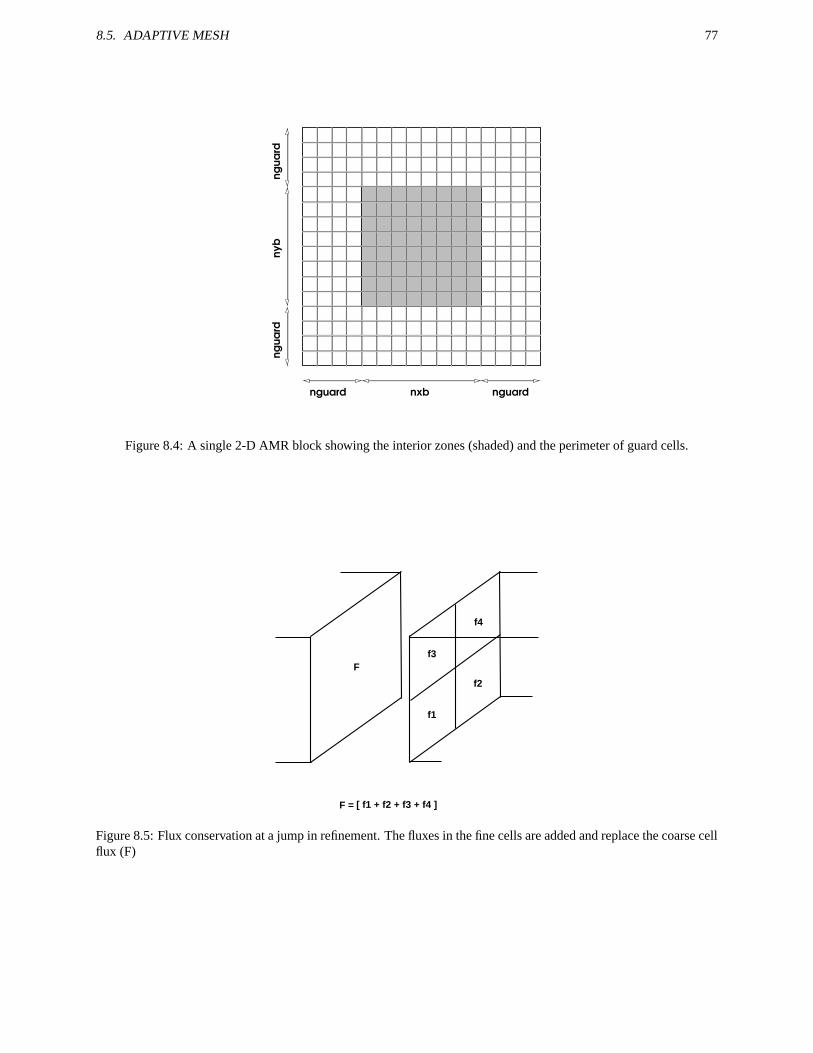
8.5. ADAPTIVE MESH 77
nguard nxb nguard
ngua
rdny
bng
uard
Figure 8.4: A single 2-D AMR block showing the interior zones (shaded) and the perimeter of guard cells.
F
f1
f2
f3
f4
F = [ f1 + f2 + f3 + f4 ]
Figure 8.5: Flux conservation at a jump in refinement. The fluxes in the fine cells are added and replace the coarse cellflux (F)
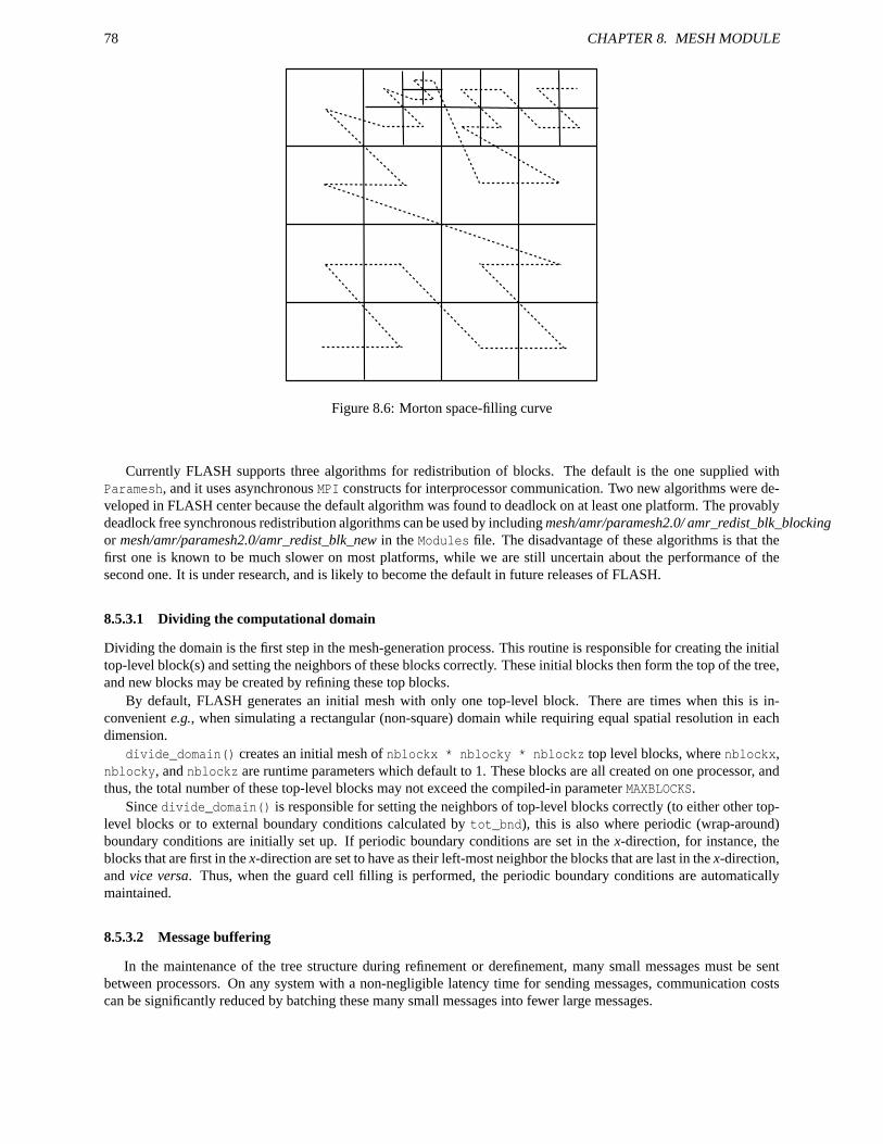
78 CHAPTER 8. MESH MODULE
Figure 8.6: Morton space-filling curve
Currently FLASH supports three algorithms for redistribution of blocks. The default is the one supplied withParamesh, and it uses asynchronous MPI constructs for interprocessor communication. Two new algorithms were de-veloped in FLASH center because the default algorithm was found to deadlock on at least one platform. The provablydeadlock free synchronous redistribution algorithms can be used by including mesh/amr/paramesh2.0/ amr_redist_blk_blockingor mesh/amr/paramesh2.0/amr_redist_blk_new in the Modules file. The disadvantage of these algorithms is that thefirst one is known to be much slower on most platforms, while we are still uncertain about the performance of thesecond one. It is under research, and is likely to become the default in future releases of FLASH.
8.5.3.1 Dividing the computational domain
Dividing the domain is the first step in the mesh-generation process. This routine is responsible for creating the initialtop-level block(s) and setting the neighbors of these blocks correctly. These initial blocks then form the top of the tree,and new blocks may be created by refining these top blocks.
By default, FLASH generates an initial mesh with only one top-level block. There are times when this is in-convenient e.g., when simulating a rectangular (non-square) domain while requiring equal spatial resolution in eachdimension.
divide_domain() creates an initial mesh of nblockx * nblocky * nblockz top level blocks, where nblockx,nblocky, and nblockz are runtime parameters which default to 1. These blocks are all created on one processor, andthus, the total number of these top-level blocks may not exceed the compiled-in parameter MAXBLOCKS.
Since divide_domain() is responsible for setting the neighbors of top-level blocks correctly (to either other top-level blocks or to external boundary conditions calculated by tot_bnd), this is also where periodic (wrap-around)boundary conditions are initially set up. If periodic boundary conditions are set in the x-direction, for instance, theblocks that are first in the x-direction are set to have as their left-most neighbor the blocks that are last in the x-direction,and vice versa. Thus, when the guard cell filling is performed, the periodic boundary conditions are automaticallymaintained.
8.5.3.2 Message buffering
In the maintenance of the tree structure during refinement or derefinement, many small messages must be sentbetween processors. On any system with a non-negligible latency time for sending messages, communication costscan be significantly reduced by batching these many small messages into fewer large messages.
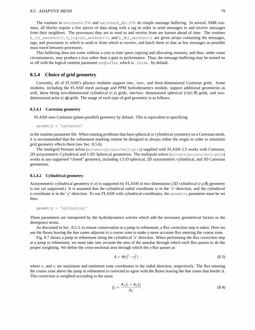
8.5. ADAPTIVE MESH 79
The routines in batchsend.F90 and batchsend_dbl.F90 do simple message buffering. In several AMR rou-tines, all blocks require a few pieces of data along with a tag in order to send messages to and receive messagesfrom their neighbors. The processors they are to send to and receive from are known ahead of time. The routinesb_int_sendrecv(), b_logical_sendrecv(), and b_dbl_sendrecv() are given arrays containing the messages,tags, and processors to which to send or from which to receive, and batch them so that as few messages as possiblemust travel between processors.
This buffering does not come without a cost in time spent copying and allocating memory, and thus, under somecircumstances, may produce a loss rather than a gain in performance. Thus, the message buffering may be turned onor off with the logical runtime parameter msgbuffer, which is .false. by default.
8.5.4 Choice of grid geometry
Currently, all of FLASH’s physics modules support one-, two-, and three-dimensional Cartesian grids. Somemodules, including the FLASH mesh package and PPM hydrodynamics module, support additional geometries aswell, these being two-dimensional cylindrical (r,z) grids, one/two- dimensional spherical (r)/(r,θ) grids, and two-dimensional polar (r,φ) grids. The usage of each type of grid geometry is as follows.
8.5.4.1 Cartesian geometry
FLASH uses Cartesian (plane-parallel) geometry by default. This is equivalent to specifying
geometry = "cartesian"
in the runtime parameter file. When running problems that have spherical or cylindrical symmetry on a Cartesian mesh,it is recommended that the refinement marking routine be designed to always refine the origin in order to minimizegrid geometry effects there (see Sec. 8.5.6).
The multigrid Poisson solver (solvers/poisson/multigrid) supplied with FLASH 2.5 works with Cartesian,2D axisymmetric Cylindrical and 1/2D Spherical geometries. The multipole solver (solvers/poisson/multipole)works in any supported “closed” geometry, including 1/2-D spherical, 2D axisymmetric cylindrical, and 3D Cartesiangeometries.
8.5.4.2 Cylindrical geometry
Axisymmetric cylindrical geometry (r,z) is supported by FLASH in two dimensions (3D cylindrical (r,z,θ) geometryis not yet supported.) It is assumed that the cylindrical radial coordinate is in the ‘x’-direction, and the cylindricalz-coordinate is in the ‘y’-direction. To run FLASH with cylindrical coordinates, the geometry parameter must be setthus:
geometry = "cylindrical"
These parameters are interpreted by the hydrodynamics solvers which add the necessary geometrical factors to thedivergence terms.
As discussed in Sec. 8.5.3, to ensure conservation at a jump in refinement, a flux correction step is taken. Here weuse the fluxes leaving the fine zones adjacent to a coarse zone to make a more accurate flux entering the coarse zone.
Fig. 8.7 shows a jump in refinement along the cylindrical ‘z’ direction. When performing the flux correction stepat a jump in refinement, we must take into account the area of the annulus through which each flux passes to do theproper weighting. We define the cross-sectional area through which the z-flux passes as
A = π(r2r − r2
l ) , (8.3)
where rr and rl are maximum and minimum zone coordinates in the radial direction, respectively. The flux enteringthe coarse zone above the jump in refinement is corrected to agree with the fluxes leaving the fine zones that border it.This correction is weighted according to the areas
f3 =A1 f1 +A2 f2
A3. (8.4)
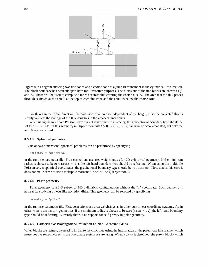
80 CHAPTER 8. MESH MODULE
block boundary
3f
f f1 2
Figure 8.7: Diagram showing two fine zones and a coarse zone at a jump in refinement in the cylindrical ‘z’ direction.The block boundary has been cut apart here for illustrative purposes. The fluxes out of the fine blocks are shown as f1
and f2. These will be used to compute a more accurate flux entering the coarse flux f3. The area that the flux passesthrough is shown as the annuli at the top of each fine zone and the annulus below the coarse zone.
For fluxes in the radial direction, the cross-sectional area is independent of the height, z, so the corrected flux issimply taken as the average of the flux densities in the adjacent finer zones.
When using the multipole Poisson solver in 2D axisymmetric geometry, the gravitational boundary type should beset to "isolated". In this geometry multipole moments ` > 0 (mpole_lmax) can now be accommodated, but only them = 0 terms are used.
8.5.4.3 Spherical geometry
One or two dimensional spherical problems can be performed by specifying
geometry = "spherical"
in the runtime parameter file. Flux corrections use area weightings as for 2D cylindrical geometry. If the minimumradius is chosen to be zero (xmin = 0.), the left-hand boundary type should be reflecting. When using the multipolePoisson solver spherical coordinates, the gravitational boundary type should be "isolated". Note that in this case itdoes not make sense to use a multipole moment ` (mpole_lmax) larger than 0.
8.5.4.4 Polar geometry
Polar geometry is a 2-D subset of 3-D cylindrical configuaration without the “z” coordinate. Such geometry isnatural for studying objects like accretion disks. This geometry can be selected by specifying
geometry = "polar"
in the runtime parameter file. Flux corrections use area weightings as in other curvilinear coordinate systems. As inother “non-cartesian” geometries, if the minimum radius is chosen to be zero (xmin = 0.), the left-hand boundarytype should be reflecting. Currently there is no support for self-gravity in polar geometry.
8.5.4.5 Conservative Prolongation/Restriction on Non-Cartesian Grids
When blocks are refined, we need to initialize the child data using the information in the parent cell in a manner whichpreserves the zone-averages in the coordinate system we are using. When a block is derefined, the parent block (which
8.5. ADAPTIVE MESH 81
is now going to be a leaf block) needs to be filled using the data in the child blocks (which are soon to be destroyed).The first procedure is called prolongation. The latter is called restriction. Both of these procedures must respect thegeometry in order to remain conservative. Prolongation and restriction are also used when filling guard cells at jumpsin refinement.
When using a supported non-Cartesian geometry, you should use the geometrically correct prolongation routines.These are:
• source/mesh/amr/paramesh2.0/quadratic_cylindrical (for cylindrical coordinates)
• source/mesh/amr/paramesh2.0/quadratic_polar (for polar coordinates)
• source/mesh/amr/paramesh2.0/quadratic_spherical (for spherical coordinates)
These routines can be included by specifying the correct path in your Modules file. Other geometry types andprolongation schemes can be added in a manner analogous to the ones implemented here.
The default restriction routines understand the supported geometries by default. A zone-volume weighted averageis used when restricting the child data up to the parent. For example, in 2-d, the restriction would look like
〈 f 〉i, j =Vic, jc 〈 f 〉ic, jc +Vic+1, jc 〈 f 〉ic+1, jc +Vic, jc+1 〈 f 〉ic, jc+1 +Vic+1, jc+1 〈 f 〉ic+1, jc+1
Vi, j, (8.5)
where Vi, j is the volume of the zone with indices, i, j, and the ic, jc indices refer to the children. In practice, wecompute the volume of the parent zone as the sum of the children to ensure conservation.
8.5.5 Using a single-level grid in PARAMESH
By default, FLASH will run a problem on an adaptive mesh, keeping the level of refinement of a block betweenlrefine_min and lrefine_max. Sometimes it is useful to run a problem with a single-level mesh. The parameshmodule can be run in a single-level ‘mode’ using the steps outlined below.
A typical problem in FLASH is set up with a single block at the top of the tree. As the refinement criteria areapplied to the initial conditions, this block and any of its children are refined to create the initial mesh. If you arerunning on a single-level grid, there is no need to carry around the entire tree hierachry, since only the leaf blocks areneeded. To get around this, you can use the divide_domain functionality (see Sec. 8.5.3.1) to create as many toplevel blocks as are needed to satisfy your resolution needs. This is accomplished by using the nblockx, nblocky, andnblockz runtime parameters to specify how many blocks to create in each direction.
Since you are placing the same resolution everywhere in the domain, it is no longer advantageous to use smallblocks. Instead, the number of zones in a block can be increased, which will reduce the memory overhead (ratioof guard cells to interior zones in a single block). When you run setup on a problem, you can set these values asarguments to setup. Currently, you cannot set nxb, nyb, and nzb as runtime parameters. Please note that some sectionsof the code assume that these quantities are even.
Be aware that while there is a benefit to having a smaller number of larger blocks, performance can suffer if youswing too far in this direction. PARAMESH does all of its load balancing based on blocks. Additionally, a block mustexist entirely on one processor. Therefore, make sure you have at least as many blocks as the number of processors onwhich you plan to run. Blocks which are too large can also result in poor cache performance.
The number of computational zones in the x-direction can be computed as
Nzonesx = nblockx×nxb (8.6)
with zones in the y and z-directions being computed similarly. Adjust nxb and nblockx to get the desired numberof zones in the x-direction (and similarly for the other coordinate directions). You can then set lrefine_max =lrefine_min = 1.
Since there will be no refinement in the problem, we prevent the code from checking for refinement by settingnrefs to zero, any negative number, or to a very large number. nrefs is the frequency (in time steps) at which tocheck the refinement criteria and defaults to 2.
Finally, since there will be no jumps in refinement, the flux conservation step is not necessary. This can beeliminated by commenting out the FLUX preprocessor definition in hydro_sweep. This will instruct the code to skipover the conservation step.
82 CHAPTER 8. MESH MODULE
8.5.6 Modifying the refinement criteria with MarkRefLib
Sometimes, it may be desirable to refine a particular region of the grid, independent of the second derivative of thevariables. This could be, for example, to better resolve the flow at the boundaries of the domain, to refine a regionwhere there is vigorous nuclear burning, or to better resolve some smooth initial condition. The MarkRefLib modulecontains methods that can refine a rectangular or circular region or using some variable threshold. It is intended to beused inside the mark_grid_refinement routine. A copy of mark_grid_refinement.F90 should be placed in thesetups directory for the problem you are working on. To use this library,
use markRefLib
should be placed in the header of the function. Then the call to the markRefInRadius, markRefInRect, or markRefVarThresholdroutine should be made in the region marked “insert user specified refinement criteria here”. We discuss the individualmethods below:
• markRefInRadiusThe general call to markRefInRadius is
call markRefInRadius(xc, yc, zc, radius, lref)
markRefInRadius takes an x (xc), y (yc), and z (zc) coordinate of the center of a sphere (circle in 2-d) and aradius (radius) and ensures that the mesh is refined up to lref levels for any blocks in that sphere (if lref> 0)or is refined once (if lref< 0).
• markRefWithRadiusThe general call to markRefWithRadius is
call markRefWithRadius(xc, yc, zc, radius, lref)
markRefWithRadius takes an x (xc), y (yc), and z (zc) coordinate of the center of a sphere (circle in 2-d), anda radius (radius) and ensures that the mesh is refined up to lref levels for any blocks containing points on thesurface of that sphere (if lref> 0) or is refined once (if lref< 0).
• markRefInRectThe general call to markRefInRect is
call markRefInRect(xlb, xrb, ylb, yrb, zlb, zrb, lref, contained)
markRefInRect refines blocks containing any points within a given rectangular region having lower left coordi-nate (xlb,ylb,zlb) and upper right coordinate (xrb,yrb,zrb). “Rectangular” is interpreted on a dimension-by-dimension basis: the region is an interval, rectangle, or rectangular parallelepiped in 1/2/3D Cartesian geometry;the rectangular cross-section of a rectangular torus in 2D axisymmetric (r− z) cylindrical geometry; an annularwedge in 2D polar (r−θ) cylindrical geometry; or an annulus in 1D spherical (r) geometry. Either blocks arebrought up to a specific level of refinement lref (if lref> 0), or each block is refined once (if lref< 0). If thecontained parameter is nonzero, only blocks completely contained within the rectangle are refined; otherwiseblocks with any overlap at all are refined.
• markRefVarThresholdTo refine on a critical value of a variable, markRefVarThreshold takes an array containing that variable in theform
real, dimension(nxb,nyb,nzb,maxblocks), :: VarVect
a threshold value for the variable (var_th), and a flag (icmp) indicating whether to refine if the variable is lessthan the threshold (icmp < 0) or greater than the threshold (icmp > 0). Any block meeting that criterion isrefined up to lref levels of refinement. The general form of the call is
call markRefVarThreshold(VarVect, var_th, icmp, lref)
• markRefOnEllipsoidSurfaceThe general call to markRefOnEllipsoidSurface is

8.5. ADAPTIVE MESH 83
call markRefOnEllipsoidSurface(x, y, z, a1, a2, a3, lref)
markRefOnEllipsoidSurface refines all blocks containing points on an ellipsoidal surface centered on (xc,yc,zc)with semimajor axes (a1,a2,a3). Either blocks are brought up to a specific level of refinement lref (if lref> 0)or each block is refined once (if lref< 0).

84 CHAPTER 8. MESH MODULE
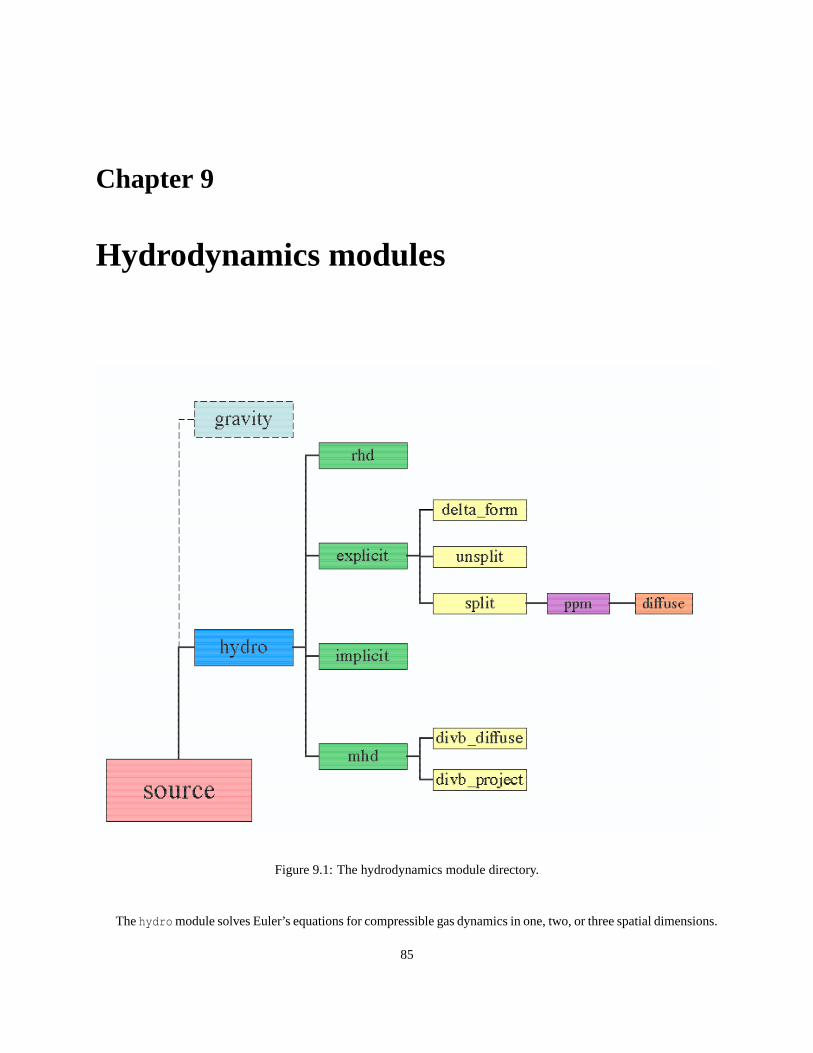
Chapter 9
Hydrodynamics modules
Figure 9.1: The hydrodynamics module directory.
The hydro module solves Euler’s equations for compressible gas dynamics in one, two, or three spatial dimensions.
85
86 CHAPTER 9. HYDRODYNAMICS MODULES
These equations can be written in conservative form as
∂ρ∂t
+∇ · (ρv) = 0 (9.1)
∂ρv∂t
+∇ · (ρvv)+∇P = ρg (9.2)
∂ρE∂t
+∇ · [(ρE +P)v] = ρv ·g , (9.3)
where ρ is the fluid density, v is the fluid velocity, P is the pressure, E is the sum of the internal energy ε and kineticenergy per unit mass,
E = ε+12|v|2 , (9.4)
g is the acceleration due to gravity, and t is the time coordinate. The pressure is obtained from the energy and densityusing the equation of state. For the case of an ideal gas equation of state, the pressure is given by
P = (γ−1)ρε , (9.5)
where γ is the ratio of specific heats. More general equations of state are discussed in Sec. 10.2.1.In regions where the kinetic energy greatly dominates the total energy, computing the internal energy using
ε = E− 12|v|2 (9.6)
can lead to unphysical values, primarily due to truncation error. This results in inaccurate pressures and temperatures.To avoid this problem, we can separately evolve the internal energy according to
∂ρε∂t
+∇ · [(ρε+P)v]−v ·∇P = 0 . (9.7)
If the internal energy is a small fraction of the kinetic energy (determined via the runtime parameter eint_switch),then the total energy is recomputed using the internal energy from eq. (9.7) and the velocities from the momentumequation. Numerical experiments using the PPM solver included with FLASH showed that using eq. (9.7) when theinternal energy falls below 10−4 of the kinetic energy helps avoid the truncation errors while not affecting the dynamicsof the simulation.
For reactive flows, a separate advection equation must be solved for each chemical or nuclear species
∂ρX`
∂t+∇ · (ρX`v) = 0 , (9.8)
where X` is the mass fraction of the `th species, with the constraint that ∑` X` = 1. FLASH will enforce this constraintif you set the runtime parameter irenorm equal to 1. Otherwise, FLASH will only restrict the abundances to fallbetween smallx and 1. The quantity ρX` represents the partial density of the `th fluid. The code does not explicitlytrack interfaces between the fluids, so a small amount of numerical mixing can be expected during the course of acalculation.
The hydro module has a capability to advect mass scalars. The mass scalars are field variables advected withdensity, similar to species mass fractions,
∂ρφ`
∂t+∇ · (ρφ`v) = 0 , (9.9)
where φ` is the `th mass scalar. Mass scalars are restricted between 0 and 1, but are not renormalized in order to sumto 1. Note that the mass scalars are optional variables; to include them one needs to specify the number of mass scalarsin problem’s Config file using NUMMASSSCALARS keyword.
All hydrodynamic modules, as well as the MHD module described in Sec. 9.4, supply the runtime parameters andsolution variables described in Tables 9.1 and 9.2. Two hydrodynamic modules are included. The first, discussed inSec. 9.1, is based on the directionally split piecewise-parabolic method (PPM) and makes use of second-order Strangtime splitting. The second, discussed in Sec. 9.2, is based on Kurganov methods and can make use of Strang splitting orRunge-Kutta time advancement. Explicit solvers such as PPM make use of the additional runtime parameter describedin Table 9.3.
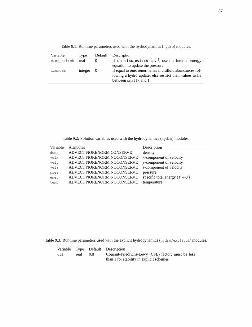
87
Table 9.1: Runtime parameters used with the hydrodynamics (hydro) modules.
Variable Type Default Descriptioneint_switch real 0 If ε < eint_switch · 1
2 |v|2, use the internal energyequation to update the pressure
irenorm integer 0 If equal to one, renormalize multifluid abundances fol-lowing a hydro update; else restrict their values to liebetween smallx and 1.
Table 9.2: Solution variables used with the hydrodynamics (hydro) modules.
Variable Attributes Descriptiondens ADVECT NORENORM CONSERVE densityvelx ADVECT NORENORM NOCONSERVE x-component of velocityvely ADVECT NORENORM NOCONSERVE y-component of velocityvelz ADVECT NORENORM NOCONSERVE z-component of velocitypres ADVECT NORENORM NOCONSERVE pressureener ADVECT NORENORM NOCONSERVE specific total energy (T +U)temp ADVECT NORENORM NOCONSERVE temperature
Table 9.3: Runtime parameters used with the explicit hydrodynamics (hydro/explicit) modules.
Variable Type Default Descriptioncfl real 0.8 Courant-Friedrichs-Lewy (CFL) factor; must be less
than 1 for stability in explicit schemes
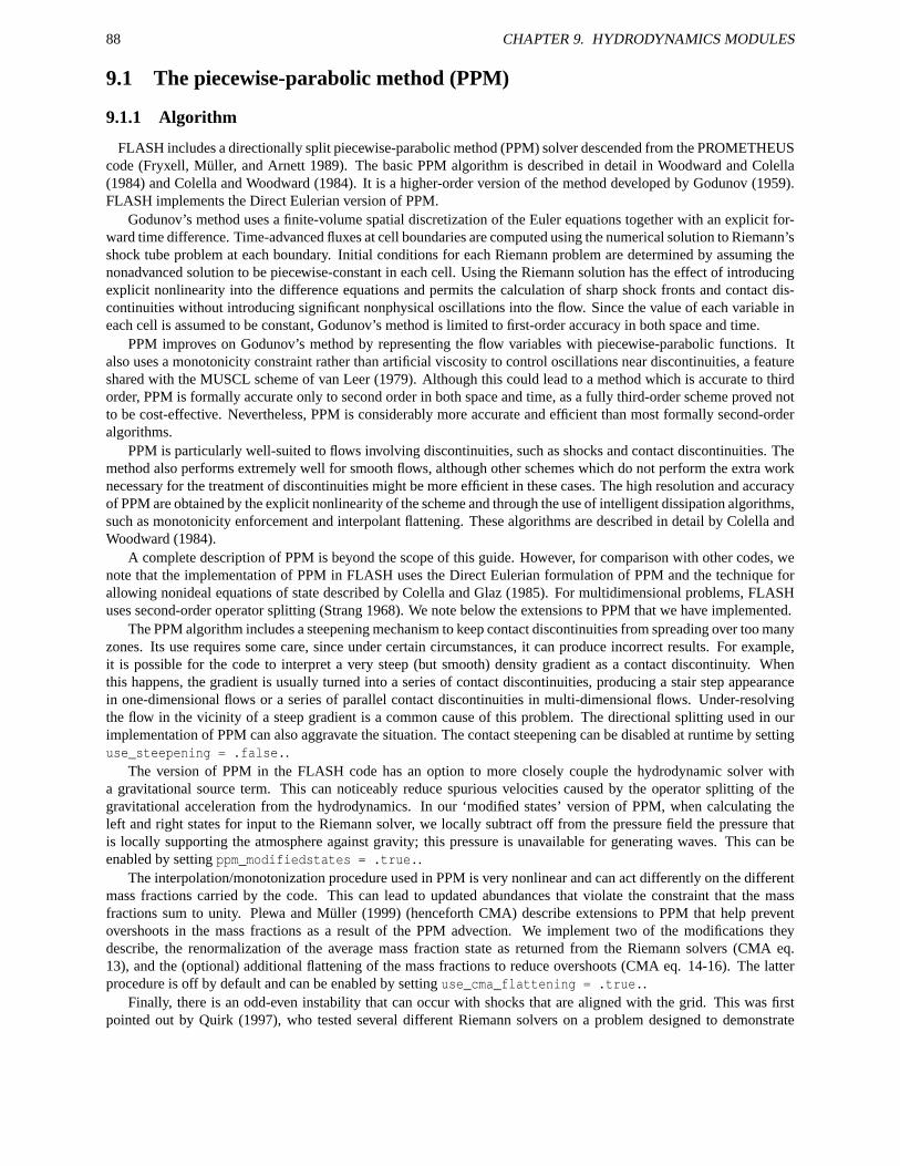
88 CHAPTER 9. HYDRODYNAMICS MODULES
9.1 The piecewise-parabolic method (PPM)
9.1.1 Algorithm
FLASH includes a directionally split piecewise-parabolic method (PPM) solver descended from the PROMETHEUScode (Fryxell, Müller, and Arnett 1989). The basic PPM algorithm is described in detail in Woodward and Colella(1984) and Colella and Woodward (1984). It is a higher-order version of the method developed by Godunov (1959).FLASH implements the Direct Eulerian version of PPM.
Godunov’s method uses a finite-volume spatial discretization of the Euler equations together with an explicit for-ward time difference. Time-advanced fluxes at cell boundaries are computed using the numerical solution to Riemann’sshock tube problem at each boundary. Initial conditions for each Riemann problem are determined by assuming thenonadvanced solution to be piecewise-constant in each cell. Using the Riemann solution has the effect of introducingexplicit nonlinearity into the difference equations and permits the calculation of sharp shock fronts and contact dis-continuities without introducing significant nonphysical oscillations into the flow. Since the value of each variable ineach cell is assumed to be constant, Godunov’s method is limited to first-order accuracy in both space and time.
PPM improves on Godunov’s method by representing the flow variables with piecewise-parabolic functions. Italso uses a monotonicity constraint rather than artificial viscosity to control oscillations near discontinuities, a featureshared with the MUSCL scheme of van Leer (1979). Although this could lead to a method which is accurate to thirdorder, PPM is formally accurate only to second order in both space and time, as a fully third-order scheme proved notto be cost-effective. Nevertheless, PPM is considerably more accurate and efficient than most formally second-orderalgorithms.
PPM is particularly well-suited to flows involving discontinuities, such as shocks and contact discontinuities. Themethod also performs extremely well for smooth flows, although other schemes which do not perform the extra worknecessary for the treatment of discontinuities might be more efficient in these cases. The high resolution and accuracyof PPM are obtained by the explicit nonlinearity of the scheme and through the use of intelligent dissipation algorithms,such as monotonicity enforcement and interpolant flattening. These algorithms are described in detail by Colella andWoodward (1984).
A complete description of PPM is beyond the scope of this guide. However, for comparison with other codes, wenote that the implementation of PPM in FLASH uses the Direct Eulerian formulation of PPM and the technique forallowing nonideal equations of state described by Colella and Glaz (1985). For multidimensional problems, FLASHuses second-order operator splitting (Strang 1968). We note below the extensions to PPM that we have implemented.
The PPM algorithm includes a steepening mechanism to keep contact discontinuities from spreading over too manyzones. Its use requires some care, since under certain circumstances, it can produce incorrect results. For example,it is possible for the code to interpret a very steep (but smooth) density gradient as a contact discontinuity. Whenthis happens, the gradient is usually turned into a series of contact discontinuities, producing a stair step appearancein one-dimensional flows or a series of parallel contact discontinuities in multi-dimensional flows. Under-resolvingthe flow in the vicinity of a steep gradient is a common cause of this problem. The directional splitting used in ourimplementation of PPM can also aggravate the situation. The contact steepening can be disabled at runtime by settinguse_steepening = .false..
The version of PPM in the FLASH code has an option to more closely couple the hydrodynamic solver witha gravitational source term. This can noticeably reduce spurious velocities caused by the operator splitting of thegravitational acceleration from the hydrodynamics. In our ‘modified states’ version of PPM, when calculating theleft and right states for input to the Riemann solver, we locally subtract off from the pressure field the pressure thatis locally supporting the atmosphere against gravity; this pressure is unavailable for generating waves. This can beenabled by setting ppm_modifiedstates = .true..
The interpolation/monotonization procedure used in PPM is very nonlinear and can act differently on the differentmass fractions carried by the code. This can lead to updated abundances that violate the constraint that the massfractions sum to unity. Plewa and Müller (1999) (henceforth CMA) describe extensions to PPM that help preventovershoots in the mass fractions as a result of the PPM advection. We implement two of the modifications theydescribe, the renormalization of the average mass fraction state as returned from the Riemann solvers (CMA eq.13), and the (optional) additional flattening of the mass fractions to reduce overshoots (CMA eq. 14-16). The latterprocedure is off by default and can be enabled by setting use_cma_flattening = .true..
Finally, there is an odd-even instability that can occur with shocks that are aligned with the grid. This was firstpointed out by Quirk (1997), who tested several different Riemann solvers on a problem designed to demonstrate
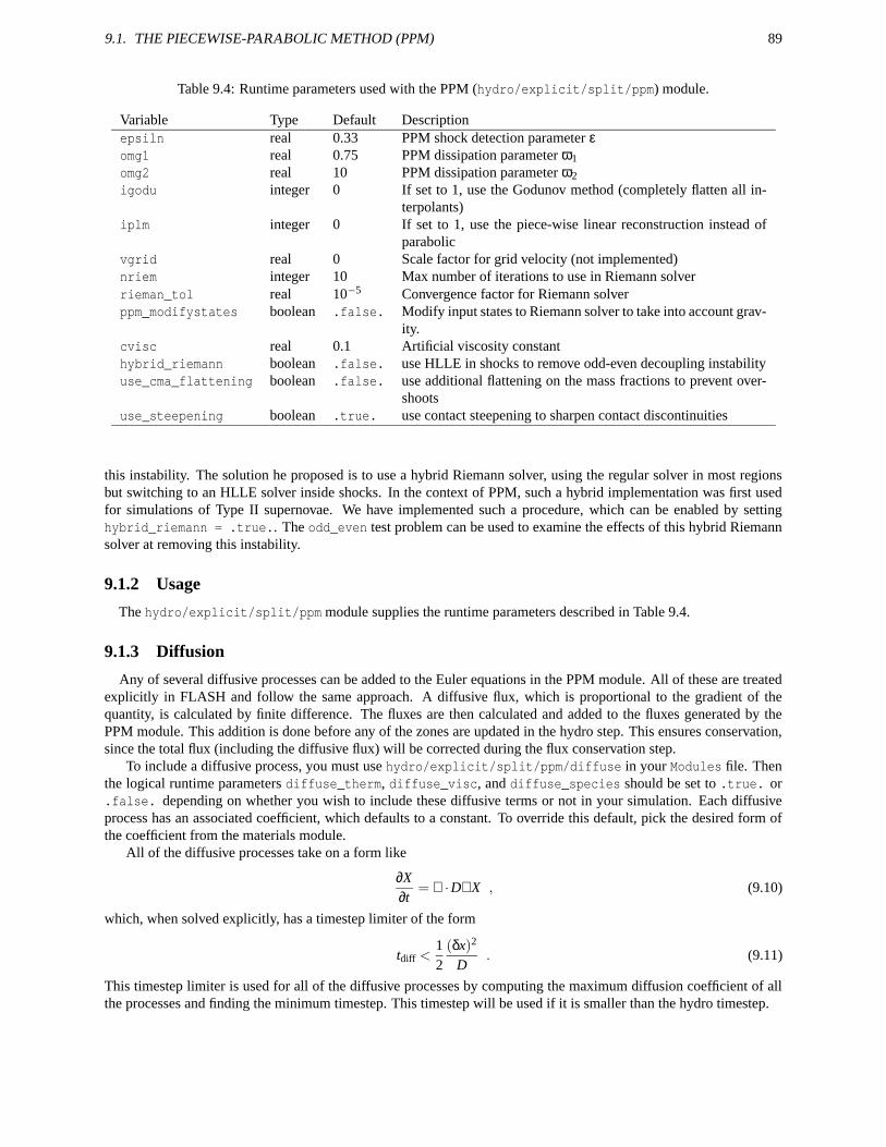
9.1. THE PIECEWISE-PARABOLIC METHOD (PPM) 89
Table 9.4: Runtime parameters used with the PPM (hydro/explicit/split/ppm) module.
Variable Type Default Descriptionepsiln real 0.33 PPM shock detection parameter εomg1 real 0.75 PPM dissipation parameter ω1
omg2 real 10 PPM dissipation parameter ω2
igodu integer 0 If set to 1, use the Godunov method (completely flatten all in-terpolants)
iplm integer 0 If set to 1, use the piece-wise linear reconstruction instead ofparabolic
vgrid real 0 Scale factor for grid velocity (not implemented)nriem integer 10 Max number of iterations to use in Riemann solverrieman_tol real 10−5 Convergence factor for Riemann solverppm_modifystates boolean .false. Modify input states to Riemann solver to take into account grav-
ity.cvisc real 0.1 Artificial viscosity constanthybrid_riemann boolean .false. use HLLE in shocks to remove odd-even decoupling instabilityuse_cma_flattening boolean .false. use additional flattening on the mass fractions to prevent over-
shootsuse_steepening boolean .true. use contact steepening to sharpen contact discontinuities
this instability. The solution he proposed is to use a hybrid Riemann solver, using the regular solver in most regionsbut switching to an HLLE solver inside shocks. In the context of PPM, such a hybrid implementation was first usedfor simulations of Type II supernovae. We have implemented such a procedure, which can be enabled by settinghybrid_riemann = .true.. The odd_even test problem can be used to examine the effects of this hybrid Riemannsolver at removing this instability.
9.1.2 Usage
The hydro/explicit/split/ppm module supplies the runtime parameters described in Table 9.4.
9.1.3 Diffusion
Any of several diffusive processes can be added to the Euler equations in the PPM module. All of these are treatedexplicitly in FLASH and follow the same approach. A diffusive flux, which is proportional to the gradient of thequantity, is calculated by finite difference. The fluxes are then calculated and added to the fluxes generated by thePPM module. This addition is done before any of the zones are updated in the hydro step. This ensures conservation,since the total flux (including the diffusive flux) will be corrected during the flux conservation step.
To include a diffusive process, you must use hydro/explicit/split/ppm/diffuse in your Modules file. Thenthe logical runtime parameters diffuse_therm, diffuse_visc, and diffuse_species should be set to .true. or.false. depending on whether you wish to include these diffusive terms or not in your simulation. Each diffusiveprocess has an associated coefficient, which defaults to a constant. To override this default, pick the desired form ofthe coefficient from the materials module.
All of the diffusive processes take on a form like
∂X∂t
= ∇ ·D∇X , (9.10)
which, when solved explicitly, has a timestep limiter of the form
tdiff <12
(δx)2
D. (9.11)
This timestep limiter is used for all of the diffusive processes by computing the maximum diffusion coefficient of allthe processes and finding the minimum timestep. This timestep will be used if it is smaller than the hydro timestep.
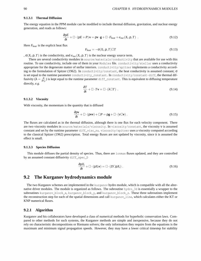
90 CHAPTER 9. HYDRODYNAMICS MODULES
9.1.3.1 Thermal Diffusion
The energy equation in the PPM module can be modified to include thermal diffusion, gravitation, and nuclear energygeneration, and reads as follows:
∂ρE∂t
+∇ · (ρE +P)v = ρv ·g+∇ ·Fheat + enuc(Xi,ρ,T ) . (9.12)
Here Fheat is the explicit heat fluxFheat =−σ(Xi,ρ,T )∇T (9.13)
, σ(Xi,ρ,T ) is the conductivity, and enuc(Xi,ρ,T ) is the nuclear energy source term.There are several conductivity modules in source/materials/conductivity that are available for use with this
routine. To use conductivity, include one of them in your Modules file. conductivity/stellar uses a conductivityappropriate for the degenerate matter of stellar interiors. conductivity/spitzer implements a conductivity accord-ing to the formulation of Spitzer (1962). In conductivity/constant, the heat conductivity is assumed constant; σis set equal to the runtime parameter conductivity_constant. In conductivity/constant-diff, the thermal dif-fusivity (λ = σ
ρcp) is kept equal to the runtime parameter diff_constant. This is equivalent to diffusing temperature
directly, e.g.∂T∂t
+∇ ·T v = ∇ · (λ∇T ) . (9.14)
9.1.3.2 Viscosity
With viscosity, the momentum is the quantity that is diffused
∂ρv∂t
+∇ · (ρvv)+∇P = ρg+∇ · (ν∇v) . (9.15)
The fluxes are calculated as in the thermal diffusion, although there is one flux for each velocity component. Thereare two viscosity modules in source/materials/viscosity. In viscosity/constant, the viscosity ν is assumedconstant and set by the runtime parameter diff_visc_nu. viscosity/spitzer uses a viscosity computed accordingto the classical Spitzer (1962) prescription. Total energy fluxes are not updated by viscosity, since it is assumed theeffect is small.
9.1.3.3 Species Diffusion
This module diffuses the partial density of species. Thus, there are ionmax fluxes updated, and they are controlledby an assumed constant diffusivity diff_spec_D
∂ρXi
∂t+∇ · (ρXiv) = ∇ · (D∇ρXi) . (9.16)
9.2 The Kurganov hydrodynamics module
The two Kurganov schemes are implemented in the kurganov hydro module, which is compatible with all the alter-native driver modules. The module is organized as follows. The subroutine hydro_3d is essentially a wrapper to thesubroutines kurganov_block_x, kurganov_block_y, and kurganov_block_z. These three subroutines implementthe reconstruction step for each of the spatial dimensions and call kurganov_line, which calculates either the KT orKNP numerical fluxes.
9.2.1 Algorithm
Kurganov and his collaborators have developed a class of numerical methods for hyperbolic conservation laws. Com-pared to other methods for such systems, the Kurganov methods are simple and inexpensive, because they do notrely on characteristic decompositions or Riemann solvers; the only information they require from the equations is themaximum and minimum signal propagation speeds. However, they may have a lower critical timestep for stability

9.2. THE KURGANOV HYDRODYNAMICS MODULE 91
and higher dissipation as a result. The Kurganov methods evolved from methods developed by Tadmor and his col-leagues, but differ in that staggered grids are used only as a device in the derivation of the schemes and are not used inthe implementation. The kurganov hydro module provides two of Kurganov’s high-resolution central schemes, eachsecond-order accurate.
There are two parts to each Kurganov method, (i) reconstruction of the conserved variables, which provides cellinterface values, and (ii) computation of the interface flux from those interface values. Various second- and third-order reconstruction algorithms have been developed; one-dimensional reconstructions can be extended dimension-by-dimension, but some multidimensional third-order reconstructions have been proposed. Two formulas are availablefor computing the fluxes from the interface values. For the first numerical flux, several wave speeds were representedby a single estimate, the maximum magnitude of the eigenvalues of the flux Jacobian (Kurganov and Tadmor 2000).Later, two estimates (maximum and minimum eigenvalues) were used, resulting in an improved numerical flux withreduced numerical dissipation (Kurganov, Noelle, and Petrova 2001).
We now describe the second-order reconstruction used in the new hydro module. The reconstruction is one-dimensional and is presented for an equispaced mesh. An arbitrary mesh cell is referred to by subscript i. The recon-struction uses the cell-averaged conserved variables Ui at nearby cells to produce values of the conserved variablesat the left and right sides of each cell interface, U l
i+ 12
and U ri+ 1
2, respectively. To update a given cell in each spatial
direction, fluxes at two interfaces must be computed; for the reconstruction used in FLASH, this update requires afive-point stencil.
The first step is to compute limited slopes, (Ux)i
(Ux)i = minmod
[
θ(Ui+1−Ui) ,θ(Ui−Ui−1) ,12
(Ui+1−Ui−1)
]
, (9.17)
where the minmod function returns the smallest argument in magnitude if all arguments are the same sign and zeroif they are not. The parameter 1 ≤ θ ≤ 2 gives some control over the limiter. The minmod limiter, which is one ofthe most diffusive, is recovered for θ = 1. The monotonized central limiter (Colella and Woodward 1984) is specifiedfor θ = 2; it is significantly less dissipative and is recommended for most cases. Other limiters may also be used tocompute the slopes; each has its pros and cons.
Once the slopes have been determined, the interface values are calculated by
U li+ 1
2= Ui +
12(Ux)i
U ri+ 1
2= Ui+1−
12(Ux)i+1 . (9.18)
Then, on each side of the interface, the speed of sound is computed. This requires the density, mass fractions, andinternal energy to be computed; then the equation of state module is called, which returns the pressure and the ratio ofspecific heats. Finally, the speeds of sound cl
i+ 12
and cri+ 1
2are computed by c = (γP/ρ)
12 .
The Kurganov-Noelle-Petrova (KNP) numerical flux is defined by
Fi+ 12
=a−
i+ 12F(U r
i+ 12)+a+
i+ 12F(U l
i+ 12)
a+i+ 1
2+a−
i+ 12
+ai+ 12
(
U ri+ 1
2−U l
i+ 12
)
, (9.19)
where for the x-direction,
a+i+ 1
2= max
(
0,uli+ 1
2+ cl
i+ 12,ur
i+ 12+ cr
i+ 12
)
(9.20)
a−i+ 1
2= − min
(
0,uli+ 1
2− cl
i+ 12,ur
i+ 12− cr
i+ 12
)
(9.21)
ai+ 12
= −(
a+i+ 1
2a−
i+ 12
)/(
a+i+ 1
2+a−
i+ 12
)
. (9.22)
Eqs. (9.20) and (9.21) are specific to the x-direction because u, the x-component of the velocity, appears; for the y- andz-directions, the appropriate velocity components, v and w, respectively should replace u.
The Kurganov-Tadmor (KT) numerical flux is
Fi+ 12
=12
[
F(U ri+ 1
2)+F(U l
i+ 12)+ai+ 1
2
(
U ri+ 1
2−U l
i+ 12
)]
, (9.23)
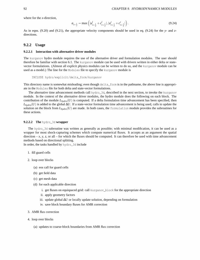
92 CHAPTER 9. HYDRODYNAMICS MODULES
where for the x-direction,
ai+ 12
= max(
|uli+ 1
2+ cl
i+ 12|, |ur
i+ 12+ cr
i+ 12|)
. (9.24)
As in eqns. (9.20) and (9.21), the appropriate velocity components should be used in eq. (9.24) for the y- and z-directions.
9.2.2 Usage
9.2.2.1 Interaction with alternative driver modules
The kurganov hydro module requires the use of the alternative driver and formulation modules. The user shouldtherefore be familiar with section 6.1. The kurganov module can be used with drivers written in either delta or state-vector formulations. (Almost all explicit physics modules can be written to do so, and the kurganov module can beused as a model.) The line for the Modules file to specify the kurganov module is
INCLUDE hydro/explicit/delta_form/kurganov
This directory name is somewhat misleading; even though delta_form is in the pathname, the above line is appropri-ate in the Modules file for both delta and state-vector formulations.
The alternative time advancement methods call hydro_3d, described in the next section, to invoke the kurganovmodule. In the context of the alternative driver modules, the hydro module does the following on each block. Thecontribution of the module Lhydro(U) is computed. If a delta formulation time advancement has been specified, thenLhydro(U) is added to the global ∆U . If a state-vector formulation time advancement is being used, calls to update thesolution on the block from Lhydro(U) are made. In both cases, the formulation module provides the subroutines forthese actions.
9.2.2.2 The hydro_3d wrapper
The hydro_3d subroutine was written as generally as possible; with minimal modification, it can be used as awrapper for most shock-capturing schemes which compute numerical fluxes. It accepts as an argument the spatialdirection – x, y, z, or all – for which the fluxes should be computed. It can therefore be used with time advancementmethods based on directional splitting.In order, the tasks handled by hydro_3d include
1. fill guard cells
2. loop over blocks
(a) eos call for guard cells
(b) get field data
(c) get mesh data
(d) for each applicable direction
i. get fluxes on equispaced grid: call kurganov_block for the appropriate direction
ii. apply geometry factors
iii. update global ∆U or locally update solution, depending on formulation
iv. save block boundary fluxes for AMR correction
3. AMR flux correction
4. loop over blocks
(a) updates to coarse-block boundaries from AMR flux correction
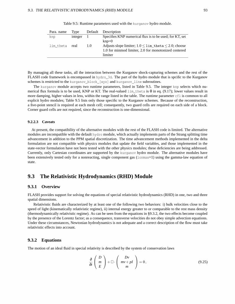
9.3. THE RELATIVISTIC HYDRODYNAMICS (RHD) MODULE 93
Table 9.5: Runtime parameters used with the kurganov hydro module.
Para. name Type Default Descriptionknp integer 1 Specifies KNP numerical flux is to be used; for KT, set
knp=0lim_theta real 1.0 Adjusts slope limiter; 1.0≤ lim_theta≤ 2.0; choose
1.0 for minmod limiter, 2.0 for monotonized centeredlimiter
By managing all these tasks, all the interaction between the Kurganov shock-capturing schemes and the rest of theFLASH code framework is encompassed in hydro_3d. The part of the hydro module that is spcific to the Kurganovschemes is restricted to the kurganov_block_[xyz] and kurganov_line subroutines.
The kurganov module accepts two runtime parameters, listed in Table 9.5. The integer knp selects which nu-merical flux formula is to be used, KNP or KT. The real-valued lim_theta is θ in eq. (9.17); lower values result inmore damping, higher values in less, within the range listed in the table. The runtime parameter cfl is common to allexplicit hydro modules; Table 9.5 lists only those specific to the Kurganov schemes. Because of the reconstruction,a five-point stencil is required at each mesh cell; consequently, two guard cells are required on each side of a block.Corner guard cells are not required, since the reconstruction is one-dimensional.
9.2.2.3 Caveats
At present, the compatibility of the alternative modules with the rest of the FLASH code is limited. The alternativemodules are incompatible with the default hydro module, which actually implements parts of the Strang splitting timeadvancement in addition to the PPM spatial discretization. The time advancement methods implemented in the deltaformulation are not compatible with physics modules that update the field variables, and those implemented in thestate-vector formulation have not been tested with the other physics modules; these deficiencies are being addressed.Currently, only Cartesian coordinates are supported by the kurganov hydro module. The alternative modules havebeen extensively tested only for a nonreacting, single component gas (ionmax=1) using the gamma-law equation ofstate.
9.3 The Relativistic Hydrodynamics (RHD) Module
9.3.1 Overview
FLASH provides support for solving the equations of special relativistic hydrodynamics (RHD) in one, two and threespatial dimensions.
Relativistic fluids are characterized by at least one of the following two behaviors: i) bulk velocities close to thespeed of light (kinematically relativistic regime), ii) internal energy greater to or comparable to the rest mass density(thermodynamically relativistic regime). As can be seen from the equations in §9.3.2, the two effects become coupledby the presence of the Lorentz factor; as a consequence, transverse velocities do not obey simple advection equations.Under these circumstances, Newtonian hydrodynamics is not adequate and a correct description of the flow must takerelativistic effects into account.
9.3.2 Equations
The motion of an ideal fluid in special relativity is described by the system of conservation laws
∂∂t
DmE
+∇ ·
Dvmv+ pI
m
= 0 , (9.25)
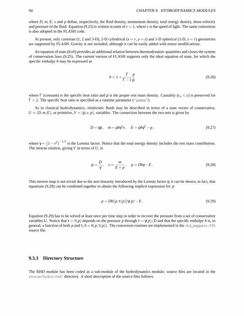
94 CHAPTER 9. HYDRODYNAMICS MODULES
where D, m, E, v and p define, respectively, the fluid density, momentum density, total energy density, three-velocityand pressure of the fluid. Equation (9.25) is written in units of c = 1, where c is the speed of light. The same conventionis also adopted in the FLASH code.
At present, only cartesian (1, 2 and 3-D), 2-D cylindrical (x = r, y = z) and 1-D spherical (1-D, x = r) geometriesare supported by FLASH. Gravity is not included, although it can be easily added with minor modifications.
An equation of state (EoS) provides an additional relation between thermodynamic quantities and closes the systemof conservation laws (9.25). The current version of FLASH supports only the ideal equation of state, for which thespecific enthalpy h may be expressed as
h = 1+Γ
Γ−1pρ
(9.26)
where Γ (constant) is the specific heat ratio and ρ is the proper rest mass density. Causality (cs < c) is preserved forΓ < 2. The specific heat ratio is specified as a runtime parameter ("gamma").
As in classical hydrodynamics, relativistic fluids may be described in terms of a state vector of conservative,U = (D,m,E), or primitive, V = (ρ,v, p), variables. The connection between the two sets is given by
D = γρ , m = ρhγ2v , E = ρhγ2− p , (9.27)
where γ =(
1− v2)−1/2
is the Lorentz factor. Notice that the total energy density includes the rest mass contribution.The inverse relation, giving V in terms of U , is
ρ =Dγ
, v =m
E + p, p = Dhγ−E . (9.28)
This inverse map is not trivial due to the non-linearity introduced by the Lorentz factor γ; it can be shown, in fact, thatequations (9.28) can be combined together to obtain the following implicit expression for p:
p = Dh(
p,τ(p))
γ(p)−E . (9.29)
Equation (9.29) has to be solved at least once per time step in order to recover the pressure from a set of conservativevariables U . Notice that τ = τ(p) depends on the pressure p through τ = γ(p)/D and that the specific enthalpy h is, ingeneral, a function of both p and τ, h = h(p,τ(p)). The conversion routines are implemented in the rhd_mappers.F90source file.
9.3.3 Directory Structure
The RHD module has been coded as a sub-module of the hydrodynamics module; source files are located in thesource/hydro/rhd/ directory. A short description of the source files follows:
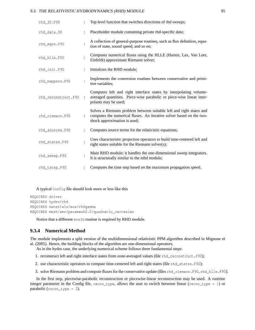
9.3. THE RELATIVISTIC HYDRODYNAMICS (RHD) MODULE 95
rhd_3D.F90 : Top level function that switches directions of rhd sweeps;
rhd_data.90 : Placeholder module containing private rhd-specific data;
rhd_eqns.F90 :A collection of general-purpose routines, such as flux definition, equa-tion of state, sound speed, and so on;
rhd_hlle.F90 :Computes numerical fluxes using the HLLE (Harten, Lax, Van Leer,Einfeldt) approximate Riemann solver;
rhd_init.F90 : Initializes the RHD module;
rhd_mappers.F90 :Implements the conversion routines between conservative and primi-tive variables;
rhd_reconstruct.F90 :Computes left and right interface states by interpolating volume-averaged quantities. Piece-wise parabolic or piece-wise linear inter-polants may be used;
rhd_riemann.F90 :Solves a Riemann problem between suitable left and right states andcomputes the numerical fluxes. An iterative solver based on the two-shock approximation is used;
rhd_sources.F90 : Computes source terms for the relativistic equations;
rhd_states.F90 :Uses characteristic projection operators to build time-centered left andright states suitable for the Riemann solver(s);
rhd_sweep.F90 :Main RHD module; it handles the one-dimensional sweep integrators.It is structurally similar to the mhd module;
rhd_tstep.F90 : Computes the time step based on the maximum propagation speed.
A typical Config file should look more or less like this
REQUIRES driverREQUIRES hydro/rhdREQUIRES materials/eos/rhdgammaREQUIRES mesh/amr/paramesh2.0/quadratic_cartesian
Notice that a different eos3d routine is required by RHD module.
9.3.4 Numerical Method
The module implements a split version of the multidimensional relativistic PPM algorithm described in Mignone etal. (2005). Hence, the building blocks of the algorithm are one-dimensional operators.
As in the hydro case, the underlying numerical scheme follows three fundamental steps:
1. reconstruct left and right interface states from zone-averaged values (file rhd_reconstruct.F90);
2. use characteristic operators to compute time-centered left and right states (file rhd_states.F90);
3. solve Riemann problem and compute fluxes for the conservative update (files rhd_riemann.F90, rhd_hlle.F90).
In the first step, piecewise-parabolic reconstruction or piecewise-linear reconstruction may be used. A runtimeinteger parameter in the Config file, recon_type, allows the user to switch between linear (recon_type = 1) orparabolic (recon_type = 2).

96 CHAPTER 9. HYDRODYNAMICS MODULES
Table 9.6: Additional solution variables used with the MHD (hydro/mhd) module.
Variable Attributes Descriptionmagx ADVECT NORENORM CONSERVE x-component of magnetic fieldmagy ADVECT NORENORM CONSERVE y-component of magnetic fieldmagz ADVECT NORENORM CONSERVE z-component of magnetic fielddivb ADVECT NORENORM NOCONSERVE divergence of magnetic field
The monotonicity constraints are essentially the same ones described in other modules and will not be repeatedhere. It should be mentioned, however, that a major complication in relativistic flows is ensuring that the total re-constructed velocity never exceeds the speed of light. In other words, caution must be taken in order to satisfyv2 = v2
x +v2y +v2
z < 1 everywhere. Therefore, in the reconstruction step an additional limiting step is applied when theprevious inequality is not fulfilled.
Second-order accuracy in time is achieved through characteristic projection operators combined with upwind lim-iting, as in the original PPM scheme (Colella & Woodward, 1984). Despite a more complex characteristic decompo-sition, the temporal evolution of the RHD equations is structurally similar to its classical counterpart. The interestedreader should consult the previous sections or the paper by Mignone et al.(2005) for a more detailed description.
In the third step, the user may choose between a non-linear iterative Riemann solver (more accurate and morecomputationally expensive) or a simple two-wave HLLE solver. Extensive calculations have shown that for highlyrelativistic flows (e.g. |v| & 0.999) the non-linear Riemann solver may fail occasionally due to strong rarefactions orshear flows. In these situations, the numerical fluxes are automatically computed using the HLLE solver. This shouldextend the applicability of the present algorithm to more extreme situations.
9.4 The magnetohydrodynamics module
9.4.1 Description
The magnetohydrodynamics module included with the FLASH code solves the equations of both ideal and non-idealMHD. As discussed in Sec. 9.4.2, the MHD module replaces the hydrodynamics module in simulations of magnetizedfluids. The two modules are conceptually very similar, and they share the same algorithmic structure. Therefore, inthe current version of the FLASH code, the MHD module is a submodule of the hydrodynamics module.
The currently released version of the MHD module uses directional splitting to evolve the equations of ideal andresistive magnetohydrodynamics. Like the hydro modules, the MHD module makes one sweep in each spatial direc-tion to advance physical variables from one time level to the next. In each sweep, the module uses AMR functionalityto fill in guard cells and impose boundary conditions. Then it reconstructs characteristic variables and uses these vari-ables to compute time-averaged interface fluxes of conserved quantities. In order to enforce conservation at jumps inrefinement, the module makes flux conservation calls to AMR, which redistributes affected fluxes using the appropriategeometric area factors. Finally, the module updates the solution and calls the EOS module to ensure thermodynamicalconsistency.
After all sweeps are completed, the MHD module enforces magnetic field divergence cleaning. Two options areavailable: diffusive and elliptic projection cleaning. In order to select a particular method, the user must, respec-tively, specify either mhd/divb_diffuse or mhd/divb_project in the problem Config file. The default methodis diffusive.
The interface of the MHD module is minimal. The module honors all of hydrodynamics module variables, interfacefunctions and runtime parameters described earlier in this chapter. In addition, it declares four global variables andthree runtime parameters, which are listed in Tables 9.6 and 9.7.
9.4.2 Algorithm
The magnetohydrodynamic (MHD) module in the FLASH code is based on a finite-volume, cell-centered methodthat was recently proposed by Powell et al. (1999). This particular choice of solver is made to comply with the data
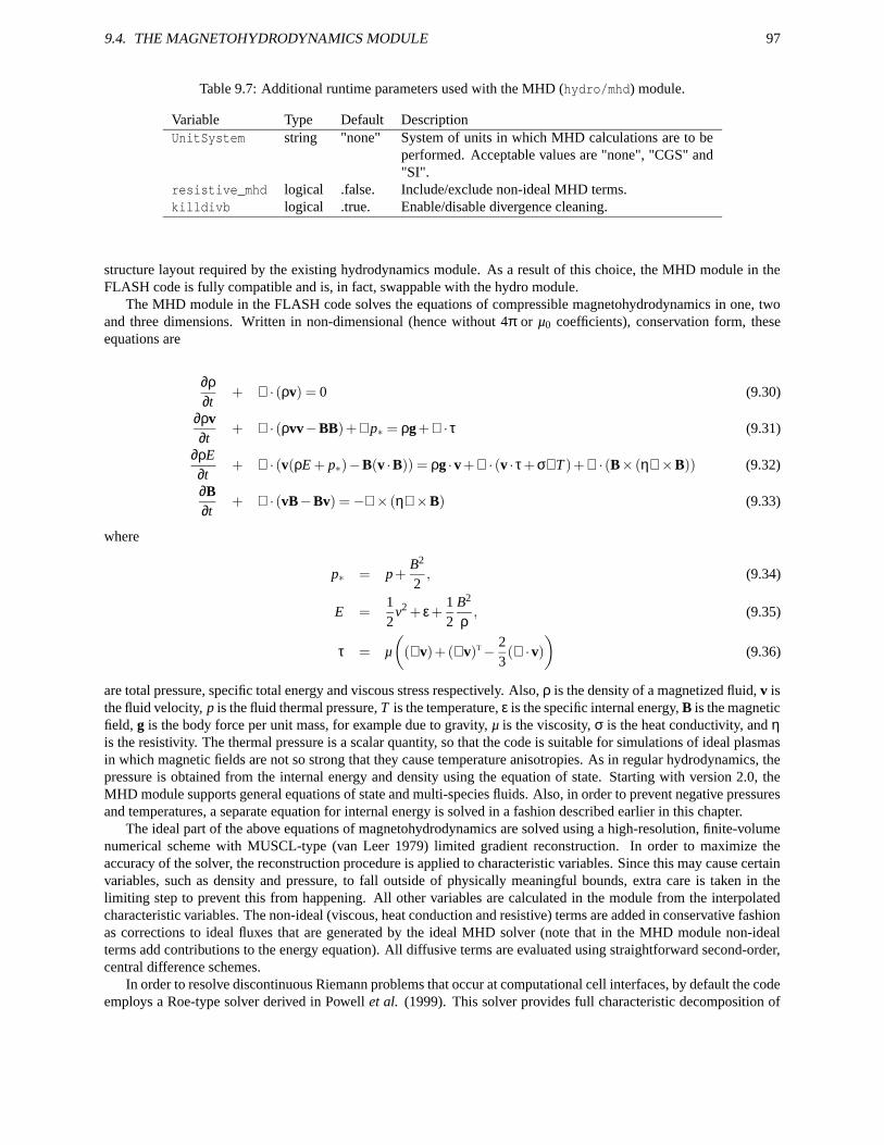
9.4. THE MAGNETOHYDRODYNAMICS MODULE 97
Table 9.7: Additional runtime parameters used with the MHD (hydro/mhd) module.
Variable Type Default DescriptionUnitSystem string "none" System of units in which MHD calculations are to be
performed. Acceptable values are "none", "CGS" and"SI".
resistive_mhd logical .false. Include/exclude non-ideal MHD terms.killdivb logical .true. Enable/disable divergence cleaning.
structure layout required by the existing hydrodynamics module. As a result of this choice, the MHD module in theFLASH code is fully compatible and is, in fact, swappable with the hydro module.
The MHD module in the FLASH code solves the equations of compressible magnetohydrodynamics in one, twoand three dimensions. Written in non-dimensional (hence without 4π or µ0 coefficients), conservation form, theseequations are
∂ρ∂t
+ ∇ · (ρv) = 0 (9.30)
∂ρv∂t
+ ∇ · (ρvv−BB)+∇p∗ = ρg+∇ · τ (9.31)
∂ρE∂t
+ ∇ · (v(ρE + p∗)−B(v ·B)) = ρg ·v+∇ · (v · τ+σ∇T )+∇ · (B× (η∇×B)) (9.32)
∂B∂t
+ ∇ · (vB−Bv) =−∇× (η∇×B) (9.33)
where
p∗ = p+B2
2, (9.34)
E =12
v2 + ε+12
B2
ρ, (9.35)
τ = µ
(
(∇v)+(∇v)T− 23(∇ ·v)
)
(9.36)
are total pressure, specific total energy and viscous stress respectively. Also, ρ is the density of a magnetized fluid, v isthe fluid velocity, p is the fluid thermal pressure, T is the temperature, ε is the specific internal energy, B is the magneticfield, g is the body force per unit mass, for example due to gravity, µ is the viscosity, σ is the heat conductivity, and ηis the resistivity. The thermal pressure is a scalar quantity, so that the code is suitable for simulations of ideal plasmasin which magnetic fields are not so strong that they cause temperature anisotropies. As in regular hydrodynamics, thepressure is obtained from the internal energy and density using the equation of state. Starting with version 2.0, theMHD module supports general equations of state and multi-species fluids. Also, in order to prevent negative pressuresand temperatures, a separate equation for internal energy is solved in a fashion described earlier in this chapter.
The ideal part of the above equations of magnetohydrodynamics are solved using a high-resolution, finite-volumenumerical scheme with MUSCL-type (van Leer 1979) limited gradient reconstruction. In order to maximize theaccuracy of the solver, the reconstruction procedure is applied to characteristic variables. Since this may cause certainvariables, such as density and pressure, to fall outside of physically meaningful bounds, extra care is taken in thelimiting step to prevent this from happening. All other variables are calculated in the module from the interpolatedcharacteristic variables. The non-ideal (viscous, heat conduction and resistive) terms are added in conservative fashionas corrections to ideal fluxes that are generated by the ideal MHD solver (note that in the MHD module non-idealterms add contributions to the energy equation). All diffusive terms are evaluated using straightforward second-order,central difference schemes.
In order to resolve discontinuous Riemann problems that occur at computational cell interfaces, by default the codeemploys a Roe-type solver derived in Powell et al. (1999). This solver provides full characteristic decomposition of
98 CHAPTER 9. HYDRODYNAMICS MODULES
the ideal MHD equations and is, therefore, particularly useful for plasma flow simulations that feature complex waveinteraction patterns. In some instances this solver may lack robustness and therefore an alternative Riemann solver ofHLLE type is provided. In order to enable this solver a Config file should require hydro/mhd/hlle. Time integrationin the MHD module is done using a second-order, one-step method due to Hancock (Toro 1997). For linear systemswith unlimited gradient reconstruction, this method can be shown to coincide with the classic Lax-Wendroff scheme.
A difficulty particularly associated with solving the MHD equations numerically lies in the solenoidality of themagnetic field. The notorious ∇ ·B = 0 condition, a strict physical law, is very hard to satisfy in discrete computations.Being only an initial condition of the MHD equations, it enters the equations indirectly and is not, therefore, guaranteedto be generally satisfied unless special algorithmic provisions are made. Without discussing this issue in much detail,which goes well beyond the scope of this user’s guide (for example, see Tóth (2000) and references therein), we willremind that there are three commonly accepted methods to enforce the ∇ ·B condition: the elliptic projection method(Brackbill and Barnes 1980), the constrained transport method (Evans and Hawley 1988), and the truncation-level errormethod (Powell et al. 1999). In the FLASH code, the truncation-error and elliptic cleaning methods are implemented.
In the truncation-error method, the solenoidality of the magnetic field is enforced by including several termsproportional to ∇ ·B. This removes the effects of unphysical magnetic tension forces parallel to the field and stimulatespassive advection of magnetic monopoles if they are spuriously created. In many applications, this method has beenshown to be an efficient and sufficient way to generate solutions of high physical quality. However, it has also beenshown (Tóth, 2000) that this method can sometimes, for example in strongly discontinuous and stagnated flows,lead to accumulation of magnetic monopoles, whose strength is sufficient to corrupt the physical quality of computedsolutions. In order to eliminate this deficiency, the FLASH code also uses a simple yet very effective method originallydue to Marder (1987) to destroy the magnetic monopoles on the scale on which they are generated. In this method, adiffusive operator proportional to ∇∇ ·B is added to the induction equation, so that the equation becomes
∂B∂t
+∇ · (vB−Bv) =−∇× (η∇×B)−v∇ ·B+ηa∇∇ ·B , (9.37)
with the artificial diffusion coefficient ηa chosen to match that of grid numerical diffusion. In the FLASH code,ηa = λ
2 ( 1∆x + 1
∆y + 1∆z )−1, where λ is the largest characteristic speed in the flow. Since the grid magnetic diffusion
Reynolds number is always on the order of unity, this operator locally destroys magnetic monopoles at the rate atwhich they are created. Recent numerical experiments (Linde and Malagoli, submitted; Powell et al. (2001)) indicatethat this approach can very effectively bring the strength of spurious magnetic monopoles to levels that are sufficientlylow that generated solutions remain physically consistent. The entire ∇ ·B control process is local and very inexpensivecompared to other methods. Moreover, one can show that this process is asymptotically convergent (Munz et al., 2000),and each of its applications is equivalent to one Jacobi iteration in solving the Poisson equation in the elliptic projectionmethod. The caveat is that this method only suppresses but does not completely eliminate magnetic monopoles.Whether this is acceptable depends on a particular physical problem.
In order to eliminate magnetic monopoles completely, the FLASH code includes an elliptic projection method.In this method, the unphysical divergence of magnetic field can be removed to any desired level down to machineprecision. This is achieved by solving a Poisson equation for a correcting scalar field, whose gradient removes con-taminated field components when subtracted from the magnetic field. The Poisson solver needed for this operation isthe multigrid solver that is also used by the gravity module.
9.4.3 Non-ideal MHD
Non-ideal MHD terms (resistive, viscous and heat conduction terms) can be enabled or disabled in FLASH at runtime via flash.par file. In order to avoid adding separate logical tests and to preserve backward compatibility withpreviously released versions of the code, all non-ideal terms in the FLASH MHD module are grouped together inthe “resistive MHD” part of the module. Among other things, this means that now resistive_mhd flag variableturns on/off resistive, viscous and heat conduction simultaneously. This is important to remember, because, unlikethat for resistivity, the default values of kinematic viscosity and thermal conductivity in FLASH are not equal to zero.Therefore, if resistive MHD part of the module is turned on, one must provide appropriate values for all transportcoefficients in the input parameter file. Section 10 discusses in detail how this should be done.
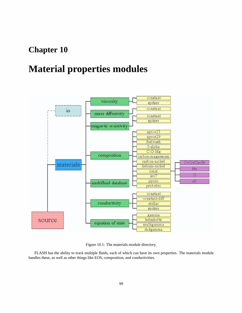
Chapter 10
Material properties modules
Figure 10.1: The materials module directory.
FLASH has the ability to track multiple fluids, each of which can have its own properties. The materials modulehandles these, as well as other things like EOS, composition, and conductivities.
99
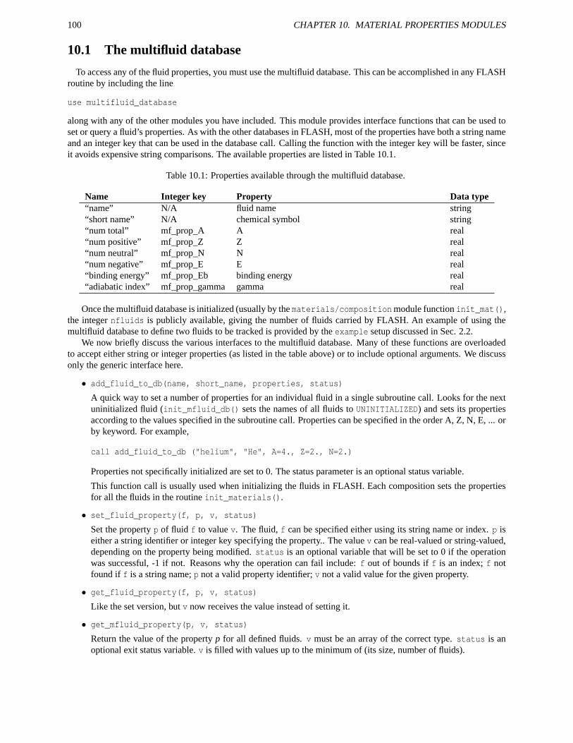
100 CHAPTER 10. MATERIAL PROPERTIES MODULES
10.1 The multifluid database
To access any of the fluid properties, you must use the multifluid database. This can be accomplished in any FLASHroutine by including the line
use multifluid_database
along with any of the other modules you have included. This module provides interface functions that can be used toset or query a fluid’s properties. As with the other databases in FLASH, most of the properties have both a string nameand an integer key that can be used in the database call. Calling the function with the integer key will be faster, sinceit avoids expensive string comparisons. The available properties are listed in Table 10.1.
Table 10.1: Properties available through the multifluid database.
Name Integer key Property Data type“name” N/A fluid name string“short name” N/A chemical symbol string“num total” mf_prop_A A real“num positive” mf_prop_Z Z real“num neutral” mf_prop_N N real“num negative” mf_prop_E E real“binding energy” mf_prop_Eb binding energy real“adiabatic index” mf_prop_gamma gamma real
Once the multifluid database is initialized (usually by the materials/compositionmodule function init_mat(),the integer nfluids is publicly available, giving the number of fluids carried by FLASH. An example of using themultifluid database to define two fluids to be tracked is provided by the example setup discussed in Sec. 2.2.
We now briefly discuss the various interfaces to the multifluid database. Many of these functions are overloadedto accept either string or integer properties (as listed in the table above) or to include optional arguments. We discussonly the generic interface here.
• add_fluid_to_db(name, short_name, properties, status)
A quick way to set a number of properties for an individual fluid in a single subroutine call. Looks for the nextuninitialized fluid (init_mfluid_db() sets the names of all fluids to UNINITIALIZED) and sets its propertiesaccording to the values specified in the subroutine call. Properties can be specified in the order A, Z, N, E, ... orby keyword. For example,
call add_fluid_to_db ("helium", "He", A=4., Z=2., N=2.)
Properties not specifically initialized are set to 0. The status parameter is an optional status variable.
This function call is usually used when initializing the fluids in FLASH. Each composition sets the propertiesfor all the fluids in the routine init_materials().
• set_fluid_property(f, p, v, status)
Set the property p of fluid f to value v. The fluid, f can be specified either using its string name or index. p iseither a string identifier or integer key specifying the property.. The value v can be real-valued or string-valued,depending on the property being modified. status is an optional variable that will be set to 0 if the operationwas successful, -1 if not. Reasons why the operation can fail include: f out of bounds if f is an index; f notfound if f is a string name; p not a valid property identifier; v not a valid value for the given property.
• get_fluid_property(f, p, v, status)
Like the set version, but v now receives the value instead of setting it.
• get_mfluid_property(p, v, status)
Return the value of the property p for all defined fluids. v must be an array of the correct type. status is anoptional exit status variable. v is filled with values up to the minimum of (its size, number of fluids).
10.2. EQUATIONS OF STATE 101
• find_fluid_index(f, i)
Find the database index i of a fluid named f. If init_mfluid_db() has not been called, or if the fluid name isnot found, this function terminates with an error. Errors are signaled by setting i to MFLUID_STATUS_FAIL.
• query_mfluid_sum(p, w, v, status)
Given a property name p and an array of weights w, return the weighted sum of the chosen property in v. wshould be an array of length equal to the number of fluids in the database or else a one-element array. If it isneither, or if the named property is invalid, the routine terminates. Typically, the weights used are the massfractions of each of the fluids in the database. The optional status variable is set to MFLUID_STATUS_OK orMFLUID_STATUS_FAIL depending on whether the summing operation was successful.
• query_mfluid_suminv(p, w, v, status)
Same as query_mfluid_sum(), but compute the weighted sum of the inverse of the chosen property.
For example, the average atomic mass of a collection of fluids is typically defined as
1A
= ∑ Xi
Aia , (10.1)
where Xi is the mass fraction of species i, and Ai is the atomic mass of that species. To compute A using themultifluid database, one would use the following lines
call query_mfluid_suminv(mf_prop_A, xn(:), abarinv, error)abar = 1.e0 / abarinv
where xn(:) is an array of the mass fractions of each species in FLASH.
• query_mfluid_sumfrc(p, w, v, status)
Same as query_mfluid_sum(), but compute the weighted sum of the chosen property divided by the totalnumber of particles (A).
• query_mfluid_sumsqr(p, w, v, status)
Same as query_mfluid_sum(), but compute the weighted sum of the square of the chosen property.
• init_mfluid_db()
Initialize the multifluid database. If this has not been called and one of the other routines is called, that routineterminates with an error. The typical FLASH user will never need to call this, since this call is part of theinit_materials() call in the composition submodule.
• list_mfluid_db(lun)
List the contents of the multifluid database in a snappy table format. Output goes to the logical I/O unit indicatedby the lun parameter.
10.2 Equations of state
The eos module implements the equation of state needed by the hydrodynamical and nuclear burning solvers.Interfaces are provided to operate on an entire block (eos3d), on a one-dimensional vector (eos1d), or for a singlezone (eos). Additionally, these functions can be used to find the thermodynamic quantities either from the density,temperature, and composition or from the density, internal energy, and composition.
Four sub-modules are available in FLASH 2.5 : gamma, which implements a perfect-gas equation of state; rhd-gamma,which implements a perfect-gas equation taking relativistic effects into account; multigamma, which implements aperfect-gas equation of state with multiple fluids, each of which can have its own adiabatic index (γ); and helmholtz,which uses a fast Helmholtz free-energy table interpolation to handle degenerate/relativistic electrons/positrons andincludes radiation pressure and ions (via the perfect gas approximation). Full details of this equation of state areprovided in Timmes & Swesty (1999).
102 CHAPTER 10. MATERIAL PROPERTIES MODULES
10.2.1 Algorithm
As described above, FLASH evolves the Euler equations for compressible, inviscid flow. This system of equationsmust be closed by an additional equation that provides a relation between the thermodynamic quantities of the gas.This is known as the equation of state for the material, and its structure and properties depend on the composition ofthe gas.
It is common to call an equation of state (henceforth EOS) routine more than 109 times during a two-dimensionalsimulation and more than 1011 times during the course of a three-dimensional simulation of stellar phenomena. Thus,it is very desirable to have an EOS that is as efficient as possible, yet accurately represents the relevant physics;considerable work can go into development of a robust and efficient EOS. While FLASH is capable of using anygeneral equation of state, we discuss here only the routines for the three equations of state that are supplied: an ideal-gas or gamma-law EOS, an EOS for a fluid composed of multiple gamma-law gases, and a tabular Helmholtz freeenergy EOS appropriate for stellar interiors. The gamma-law EOS consists of simple analytic expressions that makefor a very fast EOS routine both in the case of a single gas or for a mixture of gases. The Helmholtz EOS includesmuch more physics and relies on a table look-up scheme for performance. In this section we discuss the physics ofthese equations of state; the interfaces between the EOS routines and the codes are discussed in Sec. 10.2.2.
FLASH uses the method of Colella & Glaz (1995) to handle general equations of state. General equations ofstate contain 4 adiabatic indices (Chandrasekhar 1939), but the method of Colella & Glaz parameterizes the EOS andrequires only two of the adiabatic indices. The first is necessary to calculate the adiabatic sound speed and is given by
γ1 =Pρ
∂P∂ρ
. (10.2)
The second relates the pressure to the energy and is given by
γ4 = 1+Pρε
. (10.3)
These two adiabatic indices are stored as the variables gamc and game. All EOS routines must return γ1, and γ4 iscalculated from eq. (10.3).
The gamma-law EOS models a simple ideal gas with a constant adiabatic index γ. Here we have dropped thesubscript on γ. because for an ideal gas, all adiabatic indices are equal. The relationship between pressure P, densityρ, and specific internal energy ε is
P = (γ−1)ρε . (10.4)
We also have an expression relating pressure to the temperature T
P =Nak
AρT , (10.5)
where Na is the Avogadro number, k is the Boltzmann constant, and A is the average atomic mass, defined as
1A
= ∑i
Xi
Ai, (10.6)
where Xi is the mass fraction of the ith element. Equating these expressions for pressure yields an expression for thespecific internal energy as a function of temperature
ε =1
γ−1Nak
AT . (10.7)
The relativistic variant of the ideal gas equation is explained in more detail in Sec. 9.3.Simulations are not restricted to a single ideal gas; the multigamma EOS provides routines for simulations with
several species of ideal gases each with its own value of γ. In this case the above expressions hold, but γ represents theweighted average adiabatic index calculated from
1(γ−1)
= ∑i
1(γi−1)
Xi
Ai. (10.8)
10.2. EQUATIONS OF STATE 103
We note that the analytic expressions apply to both the forward (internal energy as a function of density, tempera-ture, and composition) and backward (temperature as a function of density, internal energy and composition) relations.Because the backward relation requires no iteration in order to obtain the temperature, this EOS is quite inexpensiveto evaluate. Despite its performance, use of the gamma-law EOS is limited, due to its restricted range of applicabilityfor astrophysical flash problems.
The Helmholtz EOS provided with the FLASH distribution contains more physics and is appropriate for addressingastrophysical phenomena in which electrons and positrons may be relativistic and/or degenerate and in which radiationmay significantly contribute to the thermodynamic state. This EOS includes contributions from radiation, completelyionized nuclei, and degenerate/relativistic electrons and positrons. The pressure and internal energy are calculated asthe sum over the components
Ptot = Prad +Pion +Pele +Ppos +Pcoul (10.9)
εtot = εrad + εion + εele + εpos + εcoul . (10.10)
Here the subscripts “rad,” “ion,” “ele,” “pos,” and “coul” represent the contributions from radiation, nuclei, electrons,positrons, and corrections for Coulomb effects, respectively. The radiation portion assumes a blackbody in localthermodynamic equilibrium, the ion portion (nuclei) is treated as an ideal gas with γ = 5/3, and the electrons andpositrons are treated as a non-interacting Fermi gas.
The blackbody pressure and energy are calculated as
Prad =aT 4
3(10.11)
εrad =3Prad
ρ(10.12)
where a is related to the Stephan-Boltzmann constant σB = ac/4, and c is the speed of light. The ion portion of eachroutine is the ideal gas of eqs. (10.4)-(10.5) with γ = 5/3. The number densities of free electrons Nele and positronsNpos in the noninteracting Fermi gas formalism are given by
Nele =8π√
2h3 m3
e c3 β3/2 [F1/2(η,β) + F3/2(η,β)]
(10.13)
Npos =8π√
2h3 m3
e c3 β3/2 [F1/2 (−η−2/β,β) + β F3/2 (−η−2/β,β)]
, (10.14)
where h is Planck’s constant, me is the electron rest mass, β = kT/(mec2) is the relativity parameter, η = µ/kT is thenormalized chemical potential energy µ for electrons, and Fk(η,β) is the Fermi-Dirac integral
Fk(η,β) =
∞∫
0
xk (1+0.5 β x)1/2 dxexp(x−η)+1
. (10.15)
Because the electron rest mass is not included in the chemical potential, the positron chemical potential must have theform ηpos = −η−2/β. For complete ionization, the number density of free electrons in the matter is
Nele,matter =Z
ANa ρ = Z Nion , (10.16)
and charge neutrality requiresNele,matter = Nele−Npos . (10.17)
Solving this equation with a standard one-dimensional root-finding algorithm determines η. Once η is known, theFermi-Dirac integrals can be evaluated, giving the pressure, specific thermal energy, and entropy due to the freeelectrons and positrons. From these, other thermodynamic quantities such as γ1 and γ4 are found. Full details of thisformalism may be found in Fryxell et al. (2000) and references therein.
The above formalism requires many complex calculations to evaluate the thermodynamic quantities, and routinesfor these calculations typically are designed for accuracy and thermodynamic consistency at the expense of speed.The Helmholtz EOS in FLASH provides a table of the Helmholtz free energy (hence the name) and makes use of a
104 CHAPTER 10. MATERIAL PROPERTIES MODULES
thermodynamically consistent interpolation scheme obviating the need to perform the complex calculations required ofthe above formalism during the course of a simulation. The interpolation scheme uses a bi-quintic Hermite interpolantresulting in an accurate EOS that performs reasonably well.
The Helmholtz free energy,F = ε−T S (10.18)
dF =−S dT +Pρ2 dρ , (10.19)
is the appropriate thermodynamic potential for use when the temperature and density are the natural thermodynamicvariables. The free energy table distributed with FLASH was produced from the Timmes EOS (Timmes & Arnett1999). The Timmes EOS evaluates the Fermi-Dirac integrals (Equation 10.15) and their partial derivatives with respectto η and β to machine precision with the efficient quadrature schemes of Aparicio (1998) and uses a Newton-Raphsoniteration to obtain the chemical potential of eq. (10.17). All partial derivatives of the pressure, entropy, and internalenergy are formed analytically. Searches through the free energy table are avoided by computing hash indices fromthe values of any given (T,ρZ/A) pair. No computationally expensive divisions are required in interpolating from thetable; all of them can be computed and stored the first time the EOS routine is called.
We note that the Helmholtz free energy table is constructed for only the electron-positron plasma, and it is a 2-dimensional function of density and temperature, i.e. F(ρ,T). It is made with A = Z = 1 (pure hydrogen), with anelectron fraction Ye = 1. One reason for not including contributions from photons and ions in the table is that thesecomponents of the Helmholtz EOS are very simple (eqs. (10.11)–(10.12)), and one doesn’t need fancy table look-upschemes to evaluate simple analytical functions. A more important reason for only constructing an electron-positronEOS table with Ye = 1 is that the 2-dimensional table is valid for any composition. Separate planes for each Ye arenot necessary (or desirable), since simple multiplication by Ye in the appropriate places gives the desired compositionscaling. If photons and ions were included in the table, then this valuable composition independence would be lost,and a 3-dimensional table would be necessary.
The Helmholtz EOS has been subjected to considerable analysis and testing (Timmes & Swesty 2000), and particu-lar care was taken to reduce the numerical error introduced by the thermodynamical models below the formal accuracyof the hydrodynamics algorithm (Fryxell, et al. 2000; Timmes & Swesty 2000). The physical limits of the HelmholtzEOS are 10−10 < ρ < 1011 (g cm−3) and 104 < T < 1011 (K). As with the gamma-law EOS, the Helmholtz EOSprovides both forward and backward relations. In the case of the forward relation (ρ,T , given along with the composi-tion) the table lookup scheme and analytic formulae directly provide relevant thermodynamic quantities. In the case ofthe backward relation (ρ,ε, and composition given), the routine performs a Newton-Rhaphson iteration to determinetemperature.
10.2.2 Usage
There are three interfaces to the EOS, reflecting the different modes in which it is used. A block interface runsthe EOS on all the zones in a block, the vector interface runs the EOS on a one-dimensional vector of zones, and apointwise interface updates the thermodynamics for a single zone. All interfaces are contained in Fortran 90 modulesto provide compile time argument checking.
10.2.2.1 The block interface, eos3d
After each update from the hydrodynamics or burning, it is necessary to update the pressure and temperature for theentire block. The eos3d function is optimized for updating all of the zones in a single block.
This function will take the density, composition, and either temperature, internal energy, or pressure as input, andreturning adiabatic indices and either the pressure, temperature or internal energy (whichever was not used as input).The input state is obtained through database calls for all of the zones in the block. eos3d takes four arguments
use ModuleEos3d
call eos3d(solnData, iblock, iflag, mode)
where solnData is one block of data, iblock is the block number to operate on, and iflag specifies which regionof the block to update. Setting iflag to 0 will update all of the interior zones (i.e. exclude guard cells). A value of
10.2. EQUATIONS OF STATE 105
7 will update all the zones in a block (interior zones + guard cells). Values between 1 and 6 update the individualregions of guard cells (upper and lower regions in the three coordinate directions). The last argument, mode specifieswhether the temperature (mode = 1), internal energy (mode = 2), or pressure (mode = 3) compliment the density andcomposition as input.
For some equations of state, it is necessary to perform a Newton-Raphson iteration to find the temperature andpressure corresponding to the internal energy, density, and composition, because the equation of state is more naturallystate in terms of temperature and density. In these cases, eos3d will do the necessary root finding up to a tolerancedefined in the function (typically 1×10⁻⁸).
10.2.2.2 The vector interface, eos1d
An alternate interface to the equation of state is provided by eos1d. This function operates on a vector, takingdensity, composition, and either temperature, internal energy, or pressure as input, and returning γ1, and either thepressure, temperature or internal energy (whichever was not used as input).
In eos1d, all the input is taken from the argument list
use ModuleEos1d
call eos1d (input, kbegin, kend, rho, tmp, p, ei, gamc, xn, q, qn)
Here, input is an integer flag that specifies whether the temperature (input = 1), internal energy (input = 2), orpressure (input = 3) compliment the density and composition as input. Two other integers, kbegin and kend specifythe beginning and ending indices in the input vectors on which to operate. The arrays rho, tmp, p, ei, and gamc areof length q, and contain the density, temperature, pressure, internal energy, and γ1, respectively. The array xn(q,qn)contains the composition (for qn fluids) for all of the input zones.
This equation of state interface is useful for initializing a problem. The user is given direct control over from wherethe input comes and where it ultimately is stored, since everything is passed through the argument list. This is moreefficient than calling the equation of state routine directly on a point by point basis, since it permits pipelining andprovides better cache performance.
10.2.2.3 The point interface, eos
The eos interface provides the most information and flexibility. No assumptions about the layout of the data aremade. This function simply takes density, composition, and either temperature or internal energy as input, and returnsa host of thermodynamic quantities. Most of the information provided here is not provided anywhere else, such as theelectron pressure, degeneracy parameter, and thermodynamic derivatives. The interface is
use ModuleEos
call eos(dens, temp, pres, ener, xn, abar, zbar, dpt, dpd, det, ded, &c_v, c_p, gammac, pel, ne, eta, input)
The arguments dens, temp, pres, and ener are the density, temperature, pressure, and internal energy respectively. xnis a vector containing the composition (the length of this vector is ionmax, supplied by the common module. abar andzbar are the average atomic mass and proton number, which are returned at the end of the call. Four thermodynamicderivatives are provided, pressure with respect to temperature (dpt) and density (dpd), and energy with respect totemperature (det) and density (ded). The specific heats at constant volume (c_v) and constant pressure (c_p) arealso provided. Finally, γ1 (gammac), the electron pressure (pel), the electron number density (ne), and the electrondegeneracy pressure (eta) are also returned. The integer input specifies whether temperature (input = 1) or internalenergy (input = 2) are used together with the density and composition as input.
10.2.2.4 Runtime parameters
There are very few runtime parameters used with these equations of state. The gamma-law EOS takes only oneparameter, the value of gamma used to relate the internal energy and pressure (see Table 10.2).
The helmholtz module also takes a single runtime parameter, which indicates whether or not to apply Coulombcorrections. In some regions of the ρ-T plane, the approximations made in the Coulomb corrections may be invalid
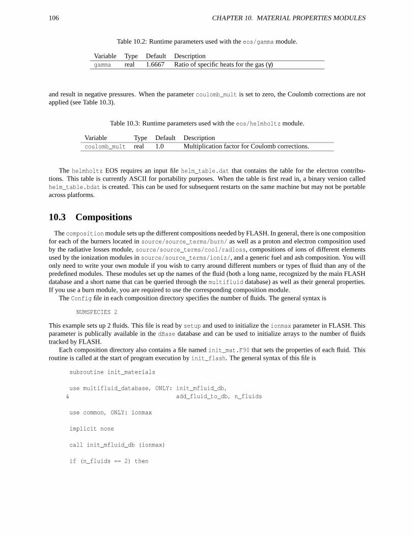
106 CHAPTER 10. MATERIAL PROPERTIES MODULES
Table 10.2: Runtime parameters used with the eos/gamma module.
Variable Type Default Descriptiongamma real 1.6667 Ratio of specific heats for the gas (γ)
and result in negative pressures. When the parameter coulomb_mult is set to zero, the Coulomb corrections are notapplied (see Table 10.3).
Table 10.3: Runtime parameters used with the eos/helmholtz module.
Variable Type Default Descriptioncoulomb_mult real 1.0 Multiplication factor for Coulomb corrections.
The helmholtz EOS requires an input file helm_table.dat that contains the table for the electron contribu-tions. This table is currently ASCII for portability purposes. When the table is first read in, a binary version calledhelm_table.bdat is created. This can be used for subsequent restarts on the same machine but may not be portableacross platforms.
10.3 Compositions
The composition module sets up the different compositions needed by FLASH. In general, there is one compositionfor each of the burners located in source/source_terms/burn/ as well as a proton and electron composition usedby the radiative losses module, source/source_terms/cool/radloss, compositions of ions of different elementsused by the ionization modules in source/source_terms/ioniz/, and a generic fuel and ash composition. You willonly need to write your own module if you wish to carry around different numbers or types of fluid than any of thepredefined modules. These modules set up the names of the fluid (both a long name, recognized by the main FLASHdatabase and a short name that can be queried through the multifluid database) as well as their general properties.If you use a burn module, you are required to use the corresponding composition module.
The Config file in each composition directory specifies the number of fluids. The general syntax is
NUMSPECIES 2
This example sets up 2 fluids. This file is read by setup and used to initialize the ionmax parameter in FLASH. Thisparameter is publically available in the dBase database and can be used to initialize arrays to the number of fluidstracked by FLASH.
Each composition directory also contains a file named init_mat.F90 that sets the properties of each fluid. Thisroutine is called at the start of program execution by init_flash. The general syntax of this file is
subroutine init_materials
use multifluid_database, ONLY: init_mfluid_db,& add_fluid_to_db, n_fluids
use common, ONLY: ionmax
implicit none
call init_mfluid_db (ionmax)
if (n_fluids == 2) then

10.3. COMPOSITIONS 107
call add_fluid_to_db ("fuel", "f", A=1., Z=1., Eb=1.)call add_fluid_to_db ("ash", "a", A=1., Z=1., Eb=1.)
else
call abort_flash("init_mat: fuel+ash requires two fluids!")
endif
returnend
Here we initialize the multifluid database through the call to init_mfluid_db. The value of ionmax is suppliedthrough the dBase database. Next, each fluid is added to the database through the calls to add_fluid_to_db, specify-ing the full name and short name, the atomic mass, proton number, and binding energy. The atomic mass and protonnumbers are used in the equations of state and are accessed via multifluid database calls.
The example setup discussed in Sec. 4.1 demonstrates how to setup a problem with two fluids (using the fuel+ashmodule). The same accessor methods that are used to store the solution data are used to store the fluid abundances ineach zone.
Below we summarize the different compositions.
10.3.1 Fuel plus ash mixture (fuel+ash)
The fuel+ash composition is not directly associated with any burner but is intended for problems that wish to tracktwo fluids, for example to study mixing.
Table 10.4: The fuel+ash composition.
Long name Short name Mass Charge Binding energyfuel f 1. 1. 1.0ash a 1. 1. 1.0
10.3.2 Minimal seven-isotope alpha-chain model (iso7)
iso7 provides a very minimal alpha-chain, useful for problems that do not have enough memory to carry a largerset of isotopes. This is the complement to the iso7 reaction network.
Table 10.5: The iso7 composition.
Long name Short name Mass Charge Binding energyhelium-4 He4 4. 2. 28.29603carbon-12 C12 12. 6. 92.16294oxygen-16 O16 16. 8. 127.62093neon-20 Ne20 20. 10. 160.64788magnesium-24 Mg24 24. 12. 198.25790silicon-28 Si28 28. 14. 236.53790nickel-56 Ni56 56. 28. 484.00300

108 CHAPTER 10. MATERIAL PROPERTIES MODULES
10.3.3 Thirteen-isotope alpha-chain model (aprox13)
aprox13 is an alpha-chain composition suitable for helium or carbon burning. It includes all of the alpha elementsup to 56Ni and is the required composition for the aprox13 network.
Table 10.6: The aprox13 composition.
Long name Short name Mass Charge Binding energyhelium-4 He4 4. 2. 28.29603carbon-12 C12 12. 6. 92.16294oxygen-16 O16 16. 8. 127.62093neon-20 Ne20 20. 10. 160.64788magnesium-24 Mg24 24. 12. 198.25790silicon-28 Si28 28. 14. 236.53790sulfur-32 S32 32. 16. 271.78250argon-36 Ar36 36. 18. 306.72020calcium-40 Ca40 40. 20. 342.05680titanium-44 Ti44 44. 22. 375.47720chromium-48 Cr48 48. 24. 411.46900iron-52 Fe52 52. 26. 447.70800nickel-56 Ni56 56. 28. 484.00300
10.3.4 Nineteen-isotope alpha-chain model (aprox19)
aprox19 builds on the aprox13 alpha-chain and adds isotopes need for pp burning, CNO and hot CNO cycles, andphotodisintegration. This composition module is required by the aprox19 reaction network.
Table 10.7: The aprox19 composition.
Long name Short name Mass Charge Binding energyhydrogen-1 H1 1. 1. 0.00000helium-3 He3 3. 2. 7.71819helium-4 He4 4. 2. 28.29603carbon-12 C12 12. 6. 92.16294nitrogen-14 N14 14. 7. 104.65998oxygen-16 O16 16. 8. 127.62093neon-20 Ne20 20. 10. 160.64788magnesium-24 Mg24 24. 12. 198.25790silicon-28 Si28 28. 14. 236.53790sulfur-32 S32 32. 16. 271.78250argon-36 Ar36 36. 18. 306.72020calcium-40 Ca40 40. 20. 342.05680titanium-44 Ti44 44. 22. 375.47720chromium-48 Cr48 48. 24. 411.46900iron-52 Fe52 52. 26. 447.70800iron-54 Fe54 54. 26. 471.76960nickel-56 Ni56 56. 28. 484.00300neutrons n 1. 0. 0.00000protons p 1. 1. 0.00000
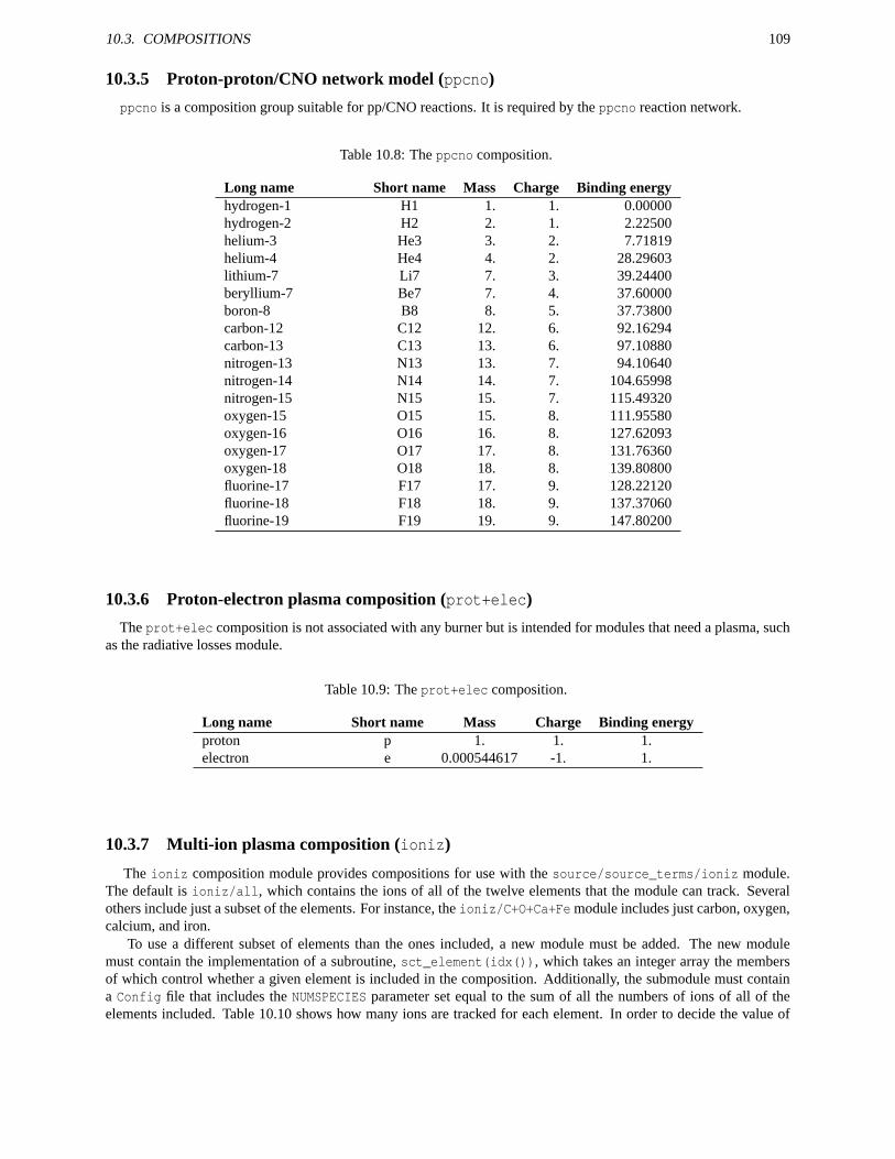
10.3. COMPOSITIONS 109
10.3.5 Proton-proton/CNO network model (ppcno)
ppcno is a composition group suitable for pp/CNO reactions. It is required by the ppcno reaction network.
Table 10.8: The ppcno composition.
Long name Short name Mass Charge Binding energyhydrogen-1 H1 1. 1. 0.00000hydrogen-2 H2 2. 1. 2.22500helium-3 He3 3. 2. 7.71819helium-4 He4 4. 2. 28.29603lithium-7 Li7 7. 3. 39.24400beryllium-7 Be7 7. 4. 37.60000boron-8 B8 8. 5. 37.73800carbon-12 C12 12. 6. 92.16294carbon-13 C13 13. 6. 97.10880nitrogen-13 N13 13. 7. 94.10640nitrogen-14 N14 14. 7. 104.65998nitrogen-15 N15 15. 7. 115.49320oxygen-15 O15 15. 8. 111.95580oxygen-16 O16 16. 8. 127.62093oxygen-17 O17 17. 8. 131.76360oxygen-18 O18 18. 8. 139.80800fluorine-17 F17 17. 9. 128.22120fluorine-18 F18 18. 9. 137.37060fluorine-19 F19 19. 9. 147.80200
10.3.6 Proton-electron plasma composition (prot+elec)
The prot+elec composition is not associated with any burner but is intended for modules that need a plasma, suchas the radiative losses module.
Table 10.9: The prot+elec composition.
Long name Short name Mass Charge Binding energyproton p 1. 1. 1.electron e 0.000544617 -1. 1.
10.3.7 Multi-ion plasma composition (ioniz)
The ioniz composition module provides compositions for use with the source/source_terms/ioniz module.The default is ioniz/all, which contains the ions of all of the twelve elements that the module can track. Severalothers include just a subset of the elements. For instance, the ioniz/C+O+Ca+Fe module includes just carbon, oxygen,calcium, and iron.
To use a different subset of elements than the ones included, a new module must be added. The new modulemust contain the implementation of a subroutine, sct_element(idx()), which takes an integer array the membersof which control whether a given element is included in the composition. Additionally, the submodule must containa Config file that includes the NUMSPECIES parameter set equal to the sum of all the numbers of ions of all of theelements included. Table 10.10 shows how many ions are tracked for each element. In order to decide the value of
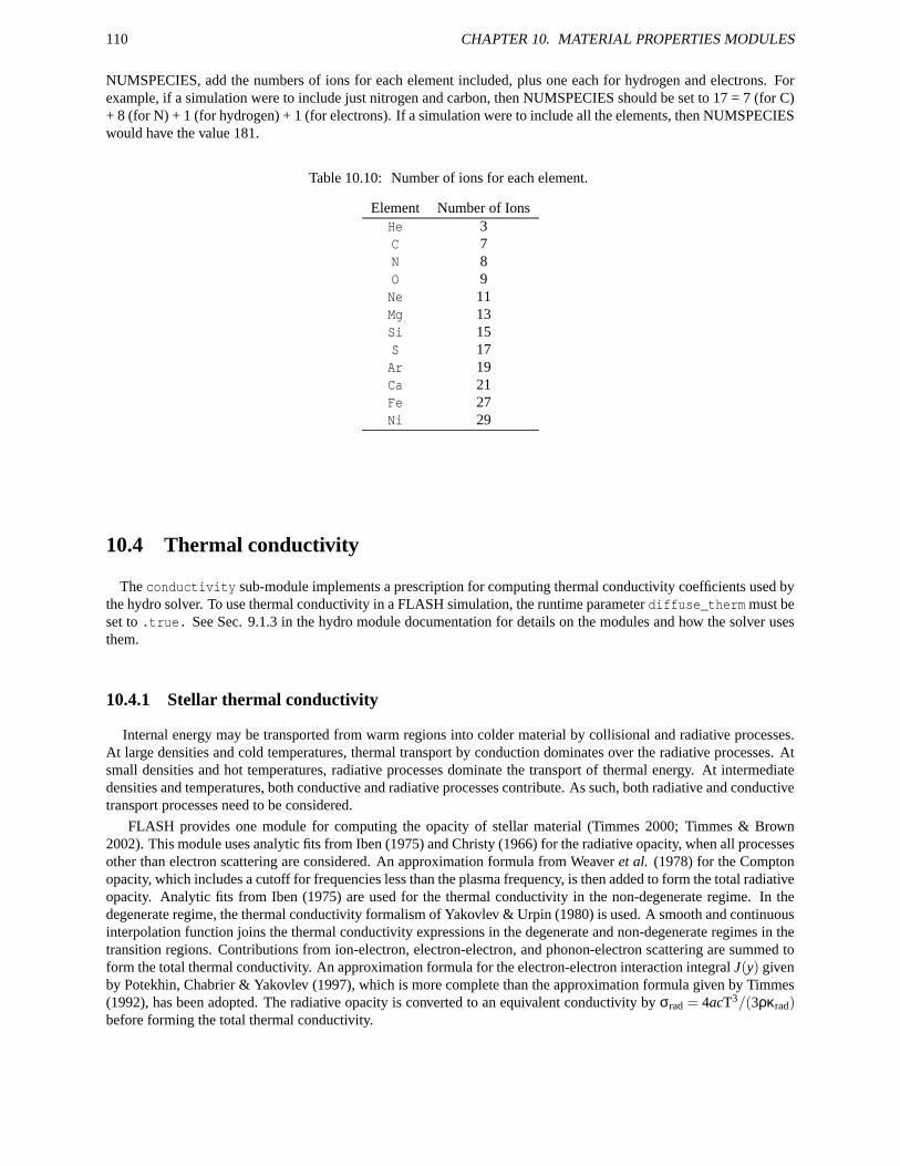
110 CHAPTER 10. MATERIAL PROPERTIES MODULES
NUMSPECIES, add the numbers of ions for each element included, plus one each for hydrogen and electrons. Forexample, if a simulation were to include just nitrogen and carbon, then NUMSPECIES should be set to 17 = 7 (for C)+ 8 (for N) + 1 (for hydrogen) + 1 (for electrons). If a simulation were to include all the elements, then NUMSPECIESwould have the value 181.
Table 10.10: Number of ions for each element.
Element Number of IonsHe 3C 7N 8O 9Ne 11Mg 13Si 15S 17Ar 19Ca 21Fe 27Ni 29
10.4 Thermal conductivity
The conductivity sub-module implements a prescription for computing thermal conductivity coefficients used bythe hydro solver. To use thermal conductivity in a FLASH simulation, the runtime parameter diffuse_therm must beset to .true. See Sec. 9.1.3 in the hydro module documentation for details on the modules and how the solver usesthem.
10.4.1 Stellar thermal conductivity
Internal energy may be transported from warm regions into colder material by collisional and radiative processes.At large densities and cold temperatures, thermal transport by conduction dominates over the radiative processes. Atsmall densities and hot temperatures, radiative processes dominate the transport of thermal energy. At intermediatedensities and temperatures, both conductive and radiative processes contribute. As such, both radiative and conductivetransport processes need to be considered.
FLASH provides one module for computing the opacity of stellar material (Timmes 2000; Timmes & Brown2002). This module uses analytic fits from Iben (1975) and Christy (1966) for the radiative opacity, when all processesother than electron scattering are considered. An approximation formula from Weaver et al. (1978) for the Comptonopacity, which includes a cutoff for frequencies less than the plasma frequency, is then added to form the total radiativeopacity. Analytic fits from Iben (1975) are used for the thermal conductivity in the non-degenerate regime. In thedegenerate regime, the thermal conductivity formalism of Yakovlev & Urpin (1980) is used. A smooth and continuousinterpolation function joins the thermal conductivity expressions in the degenerate and non-degenerate regimes in thetransition regions. Contributions from ion-electron, electron-electron, and phonon-electron scattering are summed toform the total thermal conductivity. An approximation formula for the electron-electron interaction integral J(y) givenby Potekhin, Chabrier & Yakovlev (1997), which is more complete than the approximation formula given by Timmes(1992), has been adopted. The radiative opacity is converted to an equivalent conductivity by σrad = 4acT3/(3ρκrad)before forming the total thermal conductivity.
10.5. VISCOSITY 111
10.4.2 Spitzer thermal conductivity
This module implements the thermal conductivity following the formulation of Spitzer (1962)
σ(Xi,ρ,T ) = κT n , (10.20)
where n = 5/2 and κ = 9.2×10⁻⁷ is the plasma thermal conductivity, here assumed isotropic for simplicity.
10.5 Viscosity
The viscosity sub-module implements a prescription for computing viscosity coefficients used by the hydrosolver. To use viscosity in a FLASH simulation, the runtime parameter diffus_visc must be set to .true.. See Sec.9.1.3 in the hydro module documentation for details on how the solver uses these modules.
10.5.1 Spitzer viscosity
This module implements the coefficient of plasma compressional viscosity according to the classical Spitzer (1962)prescription
ν = κT n , (10.21)
where n = 5/2 and κ = 1.25×10⁻¹⁶ (which corresponds to a Coulomb logarithm lnΛ = 20 at typical coronal condi-tions).
10.6 Magnetic resistivity and viscosity
The magnetic resistivity sub-module (source/materials/magnetic_resistivity) provides routines that com-pute magnetic resistivity η and viscosity νm for a mixture of fully ionized gases. The default top level routines returnzero values for both resistivity and viscosity. Specific routines for constant and variable resistivity are provided inconst and spitzer subdirectories. By default, all routines return results in CGS units. However they provide anoption to return results in SI units. The relationship between magnetic resistivity and viscosity is νm = c2
4π η in CGSand νm = 1
µ0η in SI.
10.6.1 Constant resistivity
This submodule returns constant magnetic resistivity and viscosity. The module declares two runtime variables,resistivity and mvisc, that are respectively the constant resistivity and viscosity. The default value for both vari-ables is zero. The magnetic resistivity function reads in resistivity and returns it to the calling routine. The mag-netic viscosity routine first checks whether mvisc is given a non-zero value in the parameter file. If it is, this non-zerovalue is returned; otherwise, the routine further reads in resistivity and converts it into magnetic viscosity.
10.6.2 Spitzer resistivity
This submodule implements the resistivity coefficient derived in Spitzer (1962)
η =e2Z lnΛ(Z)
2meγE(Z)
(πme
2kT
)32, (10.22)
where Z = ∑i niZ2i /∑i niZi is the average ionic charge of the plasma, lnΛ is the Coulomb logarithm, and γE is the
correction factor that corrects the Lorentz gas resistivity to account for electron-electron collisions. In general, thisfactor must be computed using detailed kinetic models. We fit tabulated values given in Spitzer (1962) by
γE(Z) = 0.582+0.418tanh
(
lnZ2.614
)
, 1≤ Z < ∞. (10.23)
The magnetic viscosity is computed directly from the resistivity.

112 CHAPTER 10. MATERIAL PROPERTIES MODULES
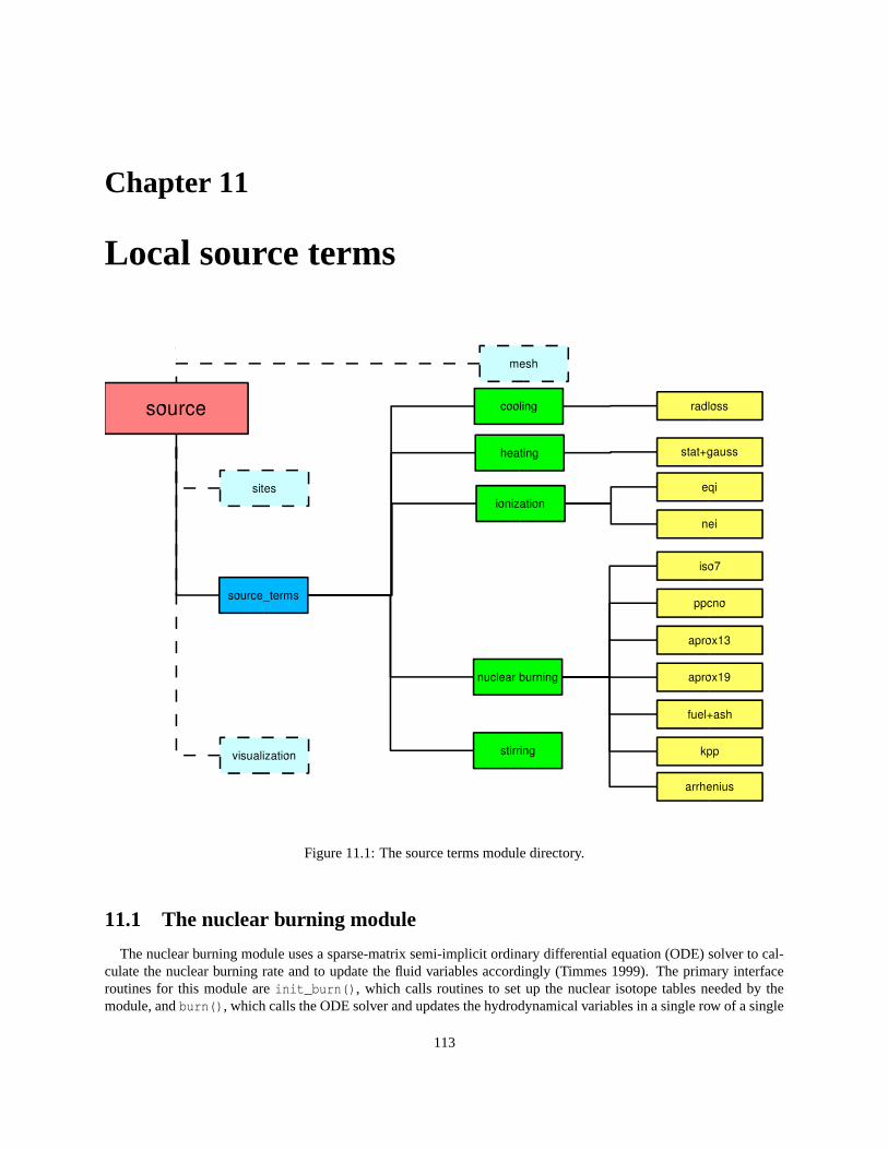
Chapter 11
Local source terms
Figure 11.1: The source terms module directory.
11.1 The nuclear burning module
The nuclear burning module uses a sparse-matrix semi-implicit ordinary differential equation (ODE) solver to cal-culate the nuclear burning rate and to update the fluid variables accordingly (Timmes 1999). The primary interfaceroutines for this module are init_burn(), which calls routines to set up the nuclear isotope tables needed by themodule, and burn(), which calls the ODE solver and updates the hydrodynamical variables in a single row of a single
113
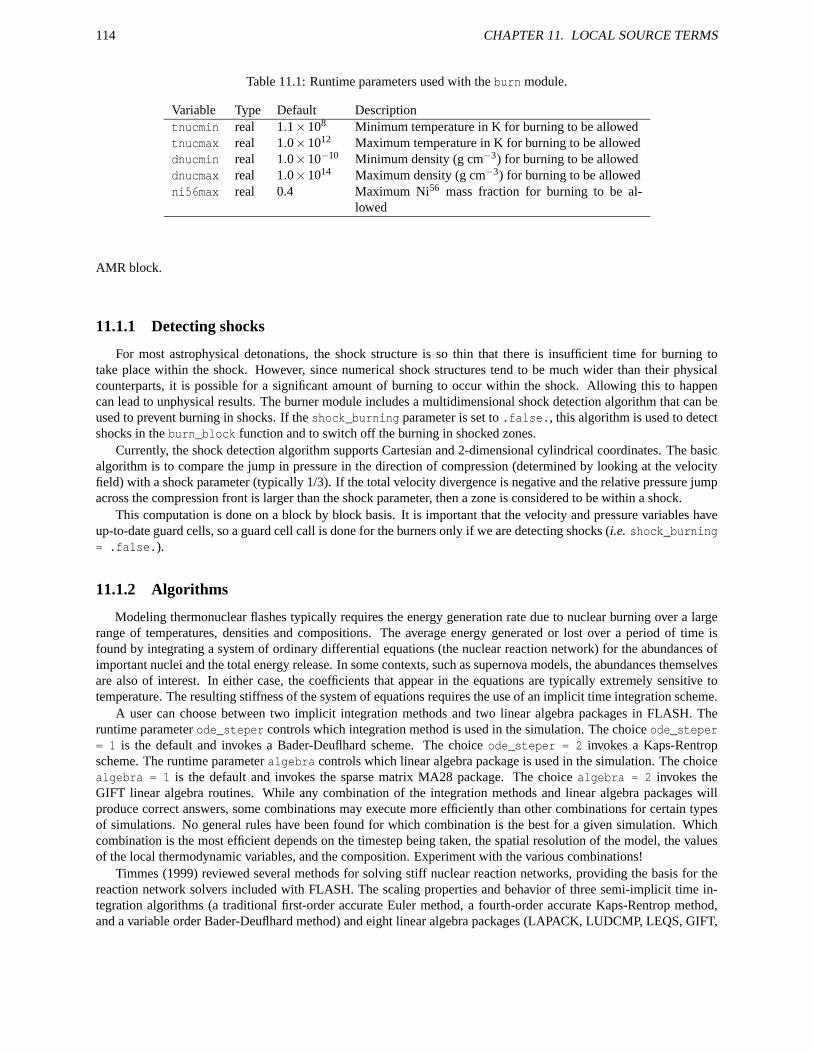
114 CHAPTER 11. LOCAL SOURCE TERMS
Table 11.1: Runtime parameters used with the burn module.
Variable Type Default Descriptiontnucmin real 1.1×10⁸ Minimum temperature in K for burning to be allowedtnucmax real 1.0×10¹² Maximum temperature in K for burning to be alloweddnucmin real 1.0×10⁻¹⁰ Minimum density (g cm−3) for burning to be alloweddnucmax real 1.0×10¹⁴ Maximum density (g cm−3) for burning to be allowedni56max real 0.4 Maximum Ni56 mass fraction for burning to be al-
lowed
AMR block.
11.1.1 Detecting shocks
For most astrophysical detonations, the shock structure is so thin that there is insufficient time for burning totake place within the shock. However, since numerical shock structures tend to be much wider than their physicalcounterparts, it is possible for a significant amount of burning to occur within the shock. Allowing this to happencan lead to unphysical results. The burner module includes a multidimensional shock detection algorithm that can beused to prevent burning in shocks. If the shock_burning parameter is set to .false., this algorithm is used to detectshocks in the burn_block function and to switch off the burning in shocked zones.
Currently, the shock detection algorithm supports Cartesian and 2-dimensional cylindrical coordinates. The basicalgorithm is to compare the jump in pressure in the direction of compression (determined by looking at the velocityfield) with a shock parameter (typically 1/3). If the total velocity divergence is negative and the relative pressure jumpacross the compression front is larger than the shock parameter, then a zone is considered to be within a shock.
This computation is done on a block by block basis. It is important that the velocity and pressure variables haveup-to-date guard cells, so a guard cell call is done for the burners only if we are detecting shocks (i.e. shock_burning= .false.).
11.1.2 Algorithms
Modeling thermonuclear flashes typically requires the energy generation rate due to nuclear burning over a largerange of temperatures, densities and compositions. The average energy generated or lost over a period of time isfound by integrating a system of ordinary differential equations (the nuclear reaction network) for the abundances ofimportant nuclei and the total energy release. In some contexts, such as supernova models, the abundances themselvesare also of interest. In either case, the coefficients that appear in the equations are typically extremely sensitive totemperature. The resulting stiffness of the system of equations requires the use of an implicit time integration scheme.
A user can choose between two implicit integration methods and two linear algebra packages in FLASH. Theruntime parameter ode_steper controls which integration method is used in the simulation. The choice ode_steper= 1 is the default and invokes a Bader-Deuflhard scheme. The choice ode_steper = 2 invokes a Kaps-Rentropscheme. The runtime parameter algebra controls which linear algebra package is used in the simulation. The choicealgebra = 1 is the default and invokes the sparse matrix MA28 package. The choice algebra = 2 invokes theGIFT linear algebra routines. While any combination of the integration methods and linear algebra packages willproduce correct answers, some combinations may execute more efficiently than other combinations for certain typesof simulations. No general rules have been found for which combination is the best for a given simulation. Whichcombination is the most efficient depends on the timestep being taken, the spatial resolution of the model, the valuesof the local thermodynamic variables, and the composition. Experiment with the various combinations!
Timmes (1999) reviewed several methods for solving stiff nuclear reaction networks, providing the basis for thereaction network solvers included with FLASH. The scaling properties and behavior of three semi-implicit time in-tegration algorithms (a traditional first-order accurate Euler method, a fourth-order accurate Kaps-Rentrop method,and a variable order Bader-Deuflhard method) and eight linear algebra packages (LAPACK, LUDCMP, LEQS, GIFT,
11.1. THE NUCLEAR BURNING MODULE 115
MA28, UMFPACK, and Y12M) were investigated by running each of these 24 combinations on seven different nu-clear reaction networks (hard-wired 13- and 19-isotope networks and soft-wired networks of 47, 76, 127, 200, and489 isotopes). Timmes’ analysis suggested that the best balance of accuracy, overall efficiency, memory footprint,and ease-of-use was provided by the two integration methods (Bader-Deuflhard and Kaps-Rentrop) and the two linearalgebra packages (MA28 and GIFT) that are provided with the FLASH code.
11.1.2.1 Reaction networks
We begin by describing the equations solved by the nuclear burning module. We consider material that may bedescribed by a density ρ and a single temperature T and contains a number of isotopes i, each of which has Zi protonsand Ai nucleons (protons + neutrons). Let ni and ρi denote the number and mass density, respectively, of the ithisotope, and let Xi denote its mass fraction, so that
Xi = ρi/ρ = niAi/(ρNA) , (11.1)
where NA is Avogadro’s number. Let the molar abundance of the ith isotope be
Yi = Xi/Ai = ni/(ρNA) . (11.2)
Mass conservation is then expressed byN
∑i=1
Xi = 1 . (11.3)
At the end of each timestep, FLASH checks that the stored abundances satisfy eq. (11.3) to machine precision inorder to avoid the unphysical buildup (or decay) of the abundances or energy generation rate. Roundoff errors in thisequation can lead to significant problems in some contexts (e.g., classical nova envelopes), where trace abundancesare important.
The general continuity equation for the ith isotope is given in Lagrangian formulation by
dYi
dt+∇ · (YiVi) = Ri . (11.4)
In this equation Ri is the total reaction rate due to all binary reactions of the form i(j,k)l,
Ri = ∑j,k
YlYkλk j(l)−YiY jλ jk(i) , (11.5)
where λk j and λ jk are the reverse (creation) and forward (destruction) nuclear reaction rates, respectively. Contribu-tions from three-body reactions, such as the triple-α reaction, are easy to append to eq. (11.5). The mass diffusionvelocities Vi in eq. (11.4) are obtained from the solution of a multicomponent diffusion equation (Chapman & Cowling1970; Burgers 1969; Williams 1988) and reflect the fact that mass diffusion processes arise from pressure, temperature,and/or abundance gradients as well as from external gravitational or electrical forces.
The case Vi ≡ 0 is important for two reasons. First, mass diffusion is often unimportant when compared to othertransport processes, such as thermal or viscous diffusion (i.e., large Lewis numbers and/or small Prandtl numbers).Such a situation obtains, for example, in the study of laminar flame fronts propagating through the quiescent interiorof a white dwarf. Second, this case permits the decoupling of the reaction network solver from the hydrodynamicalsolver through the use of operator splitting, greatly simplifying the algorithm. This is the method used by the defaultFLASH distribution. Setting Vi ≡ 0 transforms eq. (11.4) into
dYi
dt= Ri , (11.6)
which may be written in the more compact, standard form
y = f (y) . (11.7)
Stated another way, in the absence of mass diffusion or advection, any changes to the fluid composition are due tolocal processes.
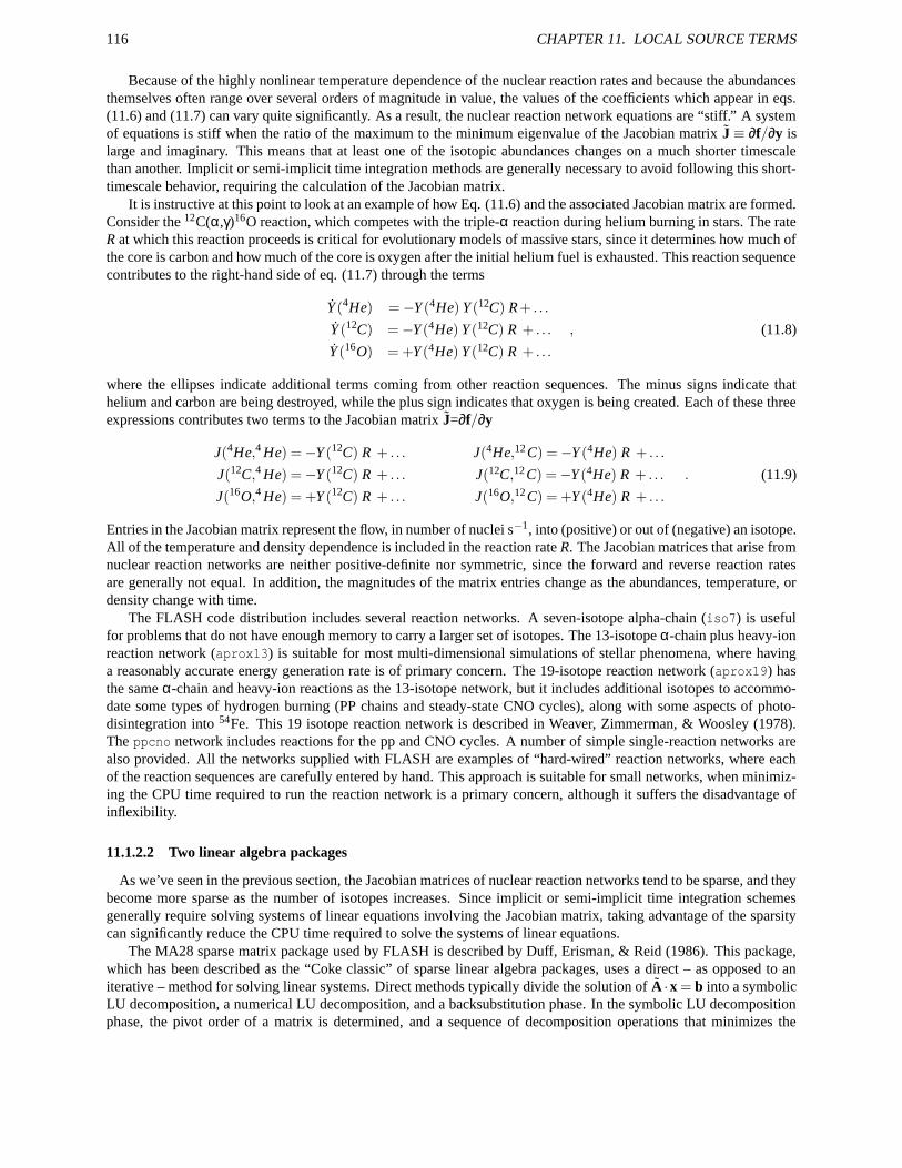
116 CHAPTER 11. LOCAL SOURCE TERMS
Because of the highly nonlinear temperature dependence of the nuclear reaction rates and because the abundancesthemselves often range over several orders of magnitude in value, the values of the coefficients which appear in eqs.(11.6) and (11.7) can vary quite significantly. As a result, the nuclear reaction network equations are “stiff.” A systemof equations is stiff when the ratio of the maximum to the minimum eigenvalue of the Jacobian matrix J ≡ ∂f/∂y islarge and imaginary. This means that at least one of the isotopic abundances changes on a much shorter timescalethan another. Implicit or semi-implicit time integration methods are generally necessary to avoid following this short-timescale behavior, requiring the calculation of the Jacobian matrix.
It is instructive at this point to look at an example of how Eq. (11.6) and the associated Jacobian matrix are formed.Consider the 12C(α,γ)16O reaction, which competes with the triple-α reaction during helium burning in stars. The rateR at which this reaction proceeds is critical for evolutionary models of massive stars, since it determines how much ofthe core is carbon and how much of the core is oxygen after the initial helium fuel is exhausted. This reaction sequencecontributes to the right-hand side of eq. (11.7) through the terms
Y (4He) =−Y (4He) Y (12C) R+ . . .
Y (12C) =−Y (4He) Y (12C) R + . . . , (11.8)
Y (16O) = +Y (4He) Y (12C) R + . . .
where the ellipses indicate additional terms coming from other reaction sequences. The minus signs indicate thathelium and carbon are being destroyed, while the plus sign indicates that oxygen is being created. Each of these threeexpressions contributes two terms to the Jacobian matrix J=∂f/∂y
J(4He,4 He) =−Y (12C) R + . . . J(4He,12 C) =−Y (4He) R + . . .
J(12C,4 He) =−Y (12C) R + . . . J(12C,12 C) =−Y (4He) R + . . . . (11.9)
J(16O,4 He) = +Y (12C) R + . . . J(16O,12 C) = +Y (4He) R + . . .
Entries in the Jacobian matrix represent the flow, in number of nuclei s−1, into (positive) or out of (negative) an isotope.All of the temperature and density dependence is included in the reaction rate R. The Jacobian matrices that arise fromnuclear reaction networks are neither positive-definite nor symmetric, since the forward and reverse reaction ratesare generally not equal. In addition, the magnitudes of the matrix entries change as the abundances, temperature, ordensity change with time.
The FLASH code distribution includes several reaction networks. A seven-isotope alpha-chain (iso7) is usefulfor problems that do not have enough memory to carry a larger set of isotopes. The 13-isotope α-chain plus heavy-ionreaction network (aprox13) is suitable for most multi-dimensional simulations of stellar phenomena, where havinga reasonably accurate energy generation rate is of primary concern. The 19-isotope reaction network (aprox19) hasthe same α-chain and heavy-ion reactions as the 13-isotope network, but it includes additional isotopes to accommo-date some types of hydrogen burning (PP chains and steady-state CNO cycles), along with some aspects of photo-disintegration into 54Fe. This 19 isotope reaction network is described in Weaver, Zimmerman, & Woosley (1978).The ppcno network includes reactions for the pp and CNO cycles. A number of simple single-reaction networks arealso provided. All the networks supplied with FLASH are examples of “hard-wired” reaction networks, where eachof the reaction sequences are carefully entered by hand. This approach is suitable for small networks, when minimiz-ing the CPU time required to run the reaction network is a primary concern, although it suffers the disadvantage ofinflexibility.
11.1.2.2 Two linear algebra packages
As we’ve seen in the previous section, the Jacobian matrices of nuclear reaction networks tend to be sparse, and theybecome more sparse as the number of isotopes increases. Since implicit or semi-implicit time integration schemesgenerally require solving systems of linear equations involving the Jacobian matrix, taking advantage of the sparsitycan significantly reduce the CPU time required to solve the systems of linear equations.
The MA28 sparse matrix package used by FLASH is described by Duff, Erisman, & Reid (1986). This package,which has been described as the “Coke classic” of sparse linear algebra packages, uses a direct – as opposed to aniterative – method for solving linear systems. Direct methods typically divide the solution of A ·x = b into a symbolicLU decomposition, a numerical LU decomposition, and a backsubstitution phase. In the symbolic LU decompositionphase, the pivot order of a matrix is determined, and a sequence of decomposition operations that minimizes the
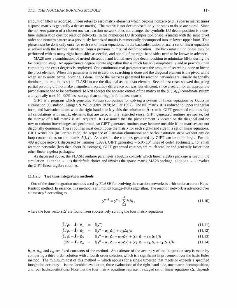
11.1. THE NUCLEAR BURNING MODULE 117
amount of fill-in is recorded. Fill-in refers to zero matrix elements which become nonzero (e.g., a sparse matrix timesa sparse matrix is generally a denser matrix). The matrix is not decomposed; only the steps to do so are stored. Sincethe nonzero pattern of a chosen nuclear reaction network does not change, the symbolic LU decomposition is a one-time initialization cost for reaction networks. In the numerical LU decomposition phase, a matrix with the same pivotorder and nonzero pattern as a previously factorized matrix is numerically decomposed into its lower-upper form. Thisphase must be done only once for each set of linear equations. In the backsubstitution phase, a set of linear equationsis solved with the factors calculated from a previous numerical decomposition. The backsubstitution phase may beperformed with as many right-hand sides as needed, and not all of the right-hand sides need to be known in advance.
MA28 uses a combination of nested dissection and frontal envelope decomposition to minimize fill-in during thefactorization stage. An approximate degree update algorithm that is much faster (asymptotically and in practice) thancomputing the exact degrees is employed. One continuous real parameter sets the amount of searching done to locatethe pivot element. When this parameter is set to zero, no searching is done and the diagonal element is the pivot, whilewhen set to unity, partial pivoting is done. Since the matrices generated by reaction networks are usually diagonallydominant, the routine is set in FLASH to use the diagonal as the pivot element. Several test cases showed that usingpartial pivoting did not make a significant accuracy difference but was less efficient, since a search for an appropriatepivot element had to be performed. MA28 accepts the nonzero entries of the matrix in the (i, j,ai, j) coordinate systemand typically uses 70−90% less storage than storing the full dense matrix.
GIFT is a program which generates Fortran subroutines for solving a system of linear equations by Gaussianelimination (Gustafson, Liniger, & Willoughby 1970; Müller 1997). The full matrix A is reduced to upper triangularform, and backsubstitution with the right-hand side b yields the solution to A · x = b. GIFT generated routines skipall calculations with matrix elements that are zero; in this restricted sense, GIFT generated routines are sparse, butthe storage of a full matrix is still required. It is assumed that the pivot element is located on the diagonal and norow or column interchanges are performed, so GIFT generated routines may become unstable if the matrices are notdiagonally dominant. These routines must decompose the matrix for each right-hand side in a set of linear equations.GIFT writes out (in Fortran code) the sequence of Gaussian elimination and backsubstitution steps without any doloop constructions on the matrix A(i, j). As a result, the routines generated by GIFT can be quite large. For the489 isotope network discussed by Timmes (1999), GIFT generated ∼ 5.0×10⁷ lines of code! Fortunately, for smallreaction networks (less than about 30 isotopes), GIFT generated routines are much smaller and generally faster thanother linear algebra packages.
As discussed above, the FLASH runtime parameter algebra controls which linear algebra package is used in thesimulation. algebra = 1 is the default choice and invokes the sparse matrix MA28 package. algebra = 2 invokesthe GIFT linear algebra routines.
11.1.2.3 Two time integration methods
One of the time integration methods used by FLASH for evolving the reaction networks is a 4th-order accurate Kaps-Rentrop method. In essence, this method is an implicit Runge-Kutta algorithm. The reaction network is advanced overa timestep h according to
yn+1 = yn +4
∑i=1
bi∆i , (11.10)
where the four vectors ∆i are found from successively solving the four matrix equations
(1/γh− J) ·∆1 = f(yn) (11.11)
(1/γh− J) ·∆2 = f(yn +a21∆1)+ c21∆1/h (11.12)
(1/γh− J) ·∆3 = f(yn +a31∆1 +a32∆2)+(c31∆1 + c32∆2)/h (11.13)
(1γh− J) ·∆4 = f(yn +a31∆1 +a32∆2)+(c41∆1 + c42∆2 + c43∆3)/h . (11.14)
bi, γ, ai j, and ci j are fixed constants of the method. An estimate of the accuracy of the integration step is made bycomparing a third-order solution with a fourth-order solution, which is a significant improvement over the basic Eulermethod. The minimum cost of this method − which applies for a single timestep that meets or exceeds a specifiedintegration accuracy − is one Jacobian evaluation, three evaluations of the right-hand side, one matrix decomposition,and four backsubstitutions. Note that the four matrix equations represent a staged set of linear equations (∆4 depends
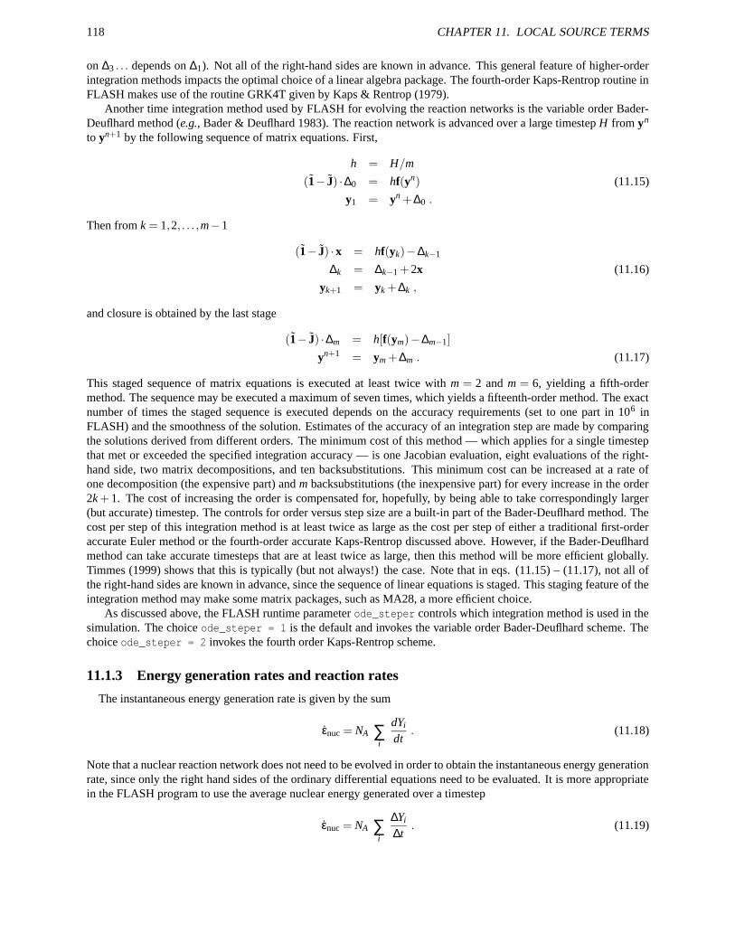
118 CHAPTER 11. LOCAL SOURCE TERMS
on ∆3 . . . depends on ∆1). Not all of the right-hand sides are known in advance. This general feature of higher-orderintegration methods impacts the optimal choice of a linear algebra package. The fourth-order Kaps-Rentrop routine inFLASH makes use of the routine GRK4T given by Kaps & Rentrop (1979).
Another time integration method used by FLASH for evolving the reaction networks is the variable order Bader-Deuflhard method (e.g., Bader & Deuflhard 1983). The reaction network is advanced over a large timestep H from yn
to yn+1 by the following sequence of matrix equations. First,
h = H/m
(1− J) ·∆0 = hf(yn) (11.15)
y1 = yn +∆0 .
Then from k = 1,2, . . . ,m−1
(1− J) ·x = hf(yk)−∆k−1
∆k = ∆k−1 +2x (11.16)
yk+1 = yk +∆k ,
and closure is obtained by the last stage
(1− J) ·∆m = h[f(ym)−∆m−1]
yn+1 = ym +∆m . (11.17)
This staged sequence of matrix equations is executed at least twice with m = 2 and m = 6, yielding a fifth-ordermethod. The sequence may be executed a maximum of seven times, which yields a fifteenth-order method. The exactnumber of times the staged sequence is executed depends on the accuracy requirements (set to one part in 106 inFLASH) and the smoothness of the solution. Estimates of the accuracy of an integration step are made by comparingthe solutions derived from different orders. The minimum cost of this method — which applies for a single timestepthat met or exceeded the specified integration accuracy — is one Jacobian evaluation, eight evaluations of the right-hand side, two matrix decompositions, and ten backsubstitutions. This minimum cost can be increased at a rate ofone decomposition (the expensive part) and m backsubstitutions (the inexpensive part) for every increase in the order2k + 1. The cost of increasing the order is compensated for, hopefully, by being able to take correspondingly larger(but accurate) timestep. The controls for order versus step size are a built-in part of the Bader-Deuflhard method. Thecost per step of this integration method is at least twice as large as the cost per step of either a traditional first-orderaccurate Euler method or the fourth-order accurate Kaps-Rentrop discussed above. However, if the Bader-Deuflhardmethod can take accurate timesteps that are at least twice as large, then this method will be more efficient globally.Timmes (1999) shows that this is typically (but not always!) the case. Note that in eqs. (11.15) – (11.17), not all ofthe right-hand sides are known in advance, since the sequence of linear equations is staged. This staging feature of theintegration method may make some matrix packages, such as MA28, a more efficient choice.
As discussed above, the FLASH runtime parameter ode_steper controls which integration method is used in thesimulation. The choice ode_steper = 1 is the default and invokes the variable order Bader-Deuflhard scheme. Thechoice ode_steper = 2 invokes the fourth order Kaps-Rentrop scheme.
11.1.3 Energy generation rates and reaction rates
The instantaneous energy generation rate is given by the sum
εnuc = NA ∑i
dYi
dt. (11.18)
Note that a nuclear reaction network does not need to be evolved in order to obtain the instantaneous energy generationrate, since only the right hand sides of the ordinary differential equations need to be evaluated. It is more appropriatein the FLASH program to use the average nuclear energy generated over a timestep
εnuc = NA ∑i
∆Yi
∆t. (11.19)
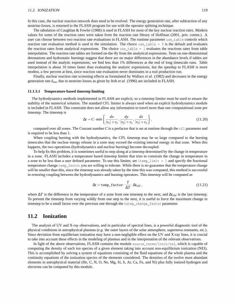
11.2. IONIZATION 119
In this case, the nuclear reaction network does need to be evolved. The energy generation rate, after subtraction of anyneutrino losses, is returned to the FLASH program for use with the operator splitting technique.
The tabulation of Caughlan & Fowler (1988) is used in FLASH for most of the key nuclear reaction rates. Modernvalues for some of the reaction rates were taken from the reaction rate library of Hoffman (2001, priv. comm.). Auser can choose between two reaction rate evaluations in FLASH. The runtime parameter use_table controls whichreaction rate evaluation method is used in the simulation. The choice use_table = 0 is the default and evaluatesthe reaction rates from analytical expressions. The choice use_table = 1 evaluates the reactions rates from tableinterpolation. The reaction rate tables are formed on-the-fly from the analytical expressions. Tests on one-dimensionaldetonations and hydrostatic burnings suggest that there are no major differences in the abundance levels if tables areused instead of the analytic expressions; we find less than 1% differences at the end of long timescale runs. Tableinterpolation is about 10 times faster than evaluating the analytic expressions, but the speedup to FLASH is moremodest, a few percent at best, since reaction rate evaluation never dominates in a real production run.
Finally, nuclear reaction rate screening effects as formulated by Wallace et al. (1982) and decreases in the energygeneration rate εnuc due to neutrino losses as given by Itoh et al. (1996) are included in FLASH.
11.1.3.1 Temperature-based timestep limiting
The hydrodynamics methods implemented in FLASH are explicit, so a timestep limiter must be used to ensure thestability of the numerical solution. The standard CFL limiter is always used when an explicit hydrodynamics moduleis included in FLASH. This constraint does not allow any information to travel more than one computational zone pertimestep. The timestep is
∆t = C ·min
dx|vx|+ cs
,dy
|vy|+ cs,
dz|vz|+ cs
, (11.20)
computed over all zones. The Courant number C is a prefactor that is set at runtime through the cfl parameter andis required to be less than 1.
When coupling burning with the hydrodynamics, the CFL timestep may be so large compared to the burningtimescales that the nuclear energy release in a zone may exceed the existing internal energy in that zone. When thishappens, the two operations (hydrodynamics and nuclear burning) become decoupled.
To help fix this problem, it is sometimes useful to step along at a timestep determined by the change in temperaturein a zone. FLASH includes a temperature based timestep limiter that tries to constrain the change in temperature ina zone to be less than a user defined parameter. To use this limiter, set itemp_limit = 1 and specify the fractionaltemperature change temp_factor you are willing to tolerate. While there is no guarantee that the temperature changewill be smaller than this, since the timestep was already taken by the time this was computed, this method is successfulin restoring coupling between the hydrodynamics and burning operators. This timestep will be computed as
∆t = temp_factor · T∆T·∆told , (11.21)
where ∆T is the difference in the temperature of a zone from one timestep to the next, and ∆told is the last timestep.To prevent the timestep from varying wildly from one step to the next, it is useful to force the maximum change intimestep to be a small factor over the previous one through the tstep_change_factor parameter.
11.2 Ionization
The analysis of UV and X-ray observations, and in particular of spectral lines, is a powerful diagnostic tool of thephysical conditions in astrophysical plasmas (e.g. the outer layers of the solar atmosphere, supernova remnants, etc.).Since deviation from equilibrium ionization may have a non-negligible effect on the UV and X-ray lines, it is crucialto take into account these effects in the modeling of plasmas and in the interpretation of the relevant observations.
In light of the above observations, FLASH contains the module source_terms/ioniz/nei, which is capable ofcomputing the density of each ion species of a given element taking into account non-equilibrium ionization (NEI).This is accomplished by solving a system of equations consisting of the fluid equations of the whole plasma and thecontinuity equations of the ionization species of the elements considered. The densities of the twelve most abundantelements in astrophysical material (He, C, N, O, Ne, Mg, Si, S, Ar, Ca, Fe, and Ni) plus fully ionized hydrogen andelectrons can be computed by this module.
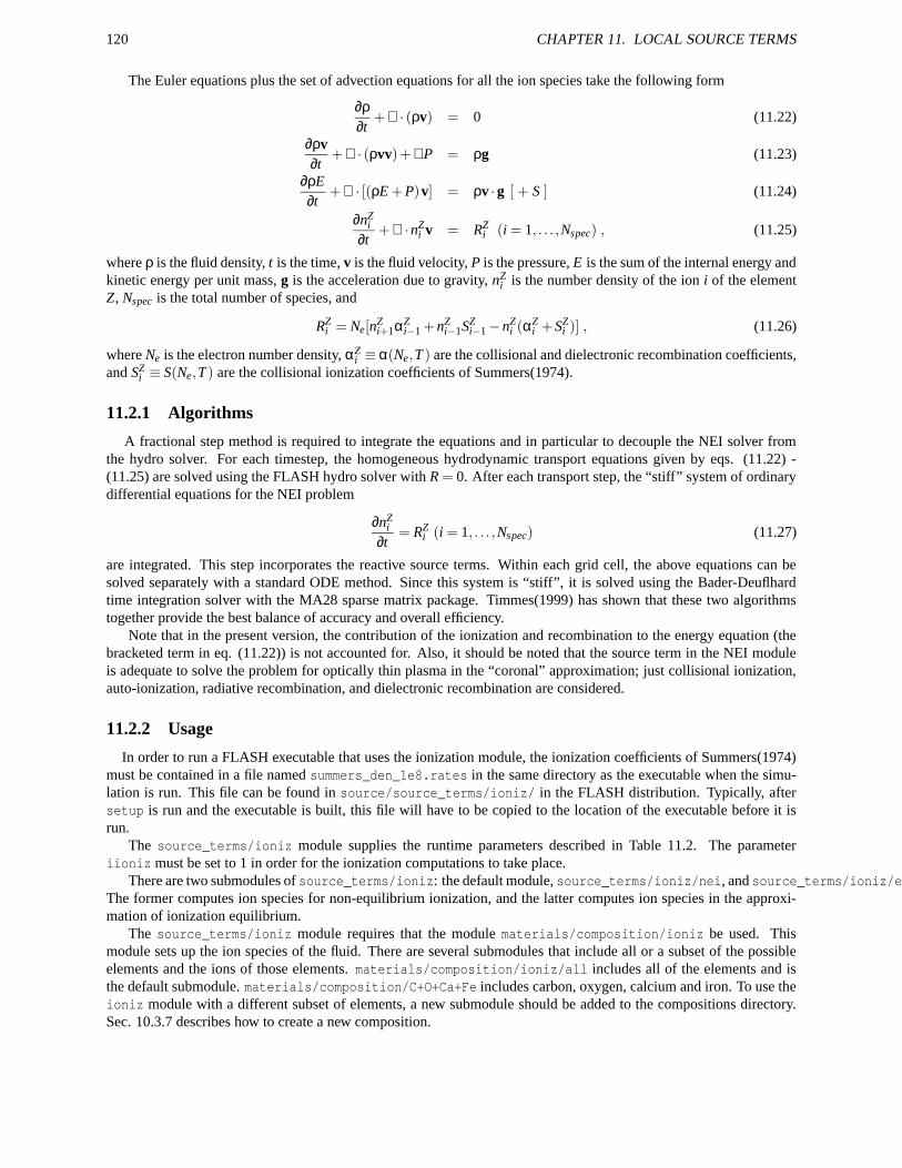
120 CHAPTER 11. LOCAL SOURCE TERMS
The Euler equations plus the set of advection equations for all the ion species take the following form
∂ρ∂t
+∇ · (ρv) = 0 (11.22)
∂ρv∂t
+∇ · (ρvv)+∇P = ρg (11.23)
∂ρE∂t
+∇ · [(ρE +P)v] = ρv ·g [ + S ] (11.24)
∂nZi
∂t+∇ ·nZ
i v = RZi (i = 1, . . . ,Nspec) , (11.25)
where ρ is the fluid density, t is the time, v is the fluid velocity, P is the pressure, E is the sum of the internal energy andkinetic energy per unit mass, g is the acceleration due to gravity, nZ
i is the number density of the ion i of the elementZ, Nspec is the total number of species, and
RZi = Ne[n
Zi+1αZ
i−1 +nZi−1SZ
i−1−nZi (αZ
i +SZi )] , (11.26)
where Ne is the electron number density, αZi ≡ α(Ne,T ) are the collisional and dielectronic recombination coefficients,
and SZi ≡ S(Ne,T ) are the collisional ionization coefficients of Summers(1974).
11.2.1 Algorithms
A fractional step method is required to integrate the equations and in particular to decouple the NEI solver fromthe hydro solver. For each timestep, the homogeneous hydrodynamic transport equations given by eqs. (11.22) -(11.25) are solved using the FLASH hydro solver with R = 0. After each transport step, the “stiff” system of ordinarydifferential equations for the NEI problem
∂nZi
∂t= RZ
i (i = 1, . . . ,Nspec) (11.27)
are integrated. This step incorporates the reactive source terms. Within each grid cell, the above equations can besolved separately with a standard ODE method. Since this system is “stiff”, it is solved using the Bader-Deuflhardtime integration solver with the MA28 sparse matrix package. Timmes(1999) has shown that these two algorithmstogether provide the best balance of accuracy and overall efficiency.
Note that in the present version, the contribution of the ionization and recombination to the energy equation (thebracketed term in eq. (11.22)) is not accounted for. Also, it should be noted that the source term in the NEI moduleis adequate to solve the problem for optically thin plasma in the “coronal” approximation; just collisional ionization,auto-ionization, radiative recombination, and dielectronic recombination are considered.
11.2.2 Usage
In order to run a FLASH executable that uses the ionization module, the ionization coefficients of Summers(1974)must be contained in a file named summers_den_1e8.rates in the same directory as the executable when the simu-lation is run. This file can be found in source/source_terms/ioniz/ in the FLASH distribution. Typically, aftersetup is run and the executable is built, this file will have to be copied to the location of the executable before it isrun.
The source_terms/ioniz module supplies the runtime parameters described in Table 11.2. The parameteriioniz must be set to 1 in order for the ionization computations to take place.
There are two submodules of source_terms/ioniz: the default module, source_terms/ioniz/nei, and source_terms/ioniz/eqi.The former computes ion species for non-equilibrium ionization, and the latter computes ion species in the approxi-mation of ionization equilibrium.
The source_terms/ioniz module requires that the module materials/composition/ioniz be used. Thismodule sets up the ion species of the fluid. There are several submodules that include all or a subset of the possibleelements and the ions of those elements. materials/composition/ioniz/all includes all of the elements and isthe default submodule. materials/composition/C+O+Ca+Fe includes carbon, oxygen, calcium and iron. To use theioniz module with a different subset of elements, a new submodule should be added to the compositions directory.Sec. 10.3.7 describes how to create a new composition.
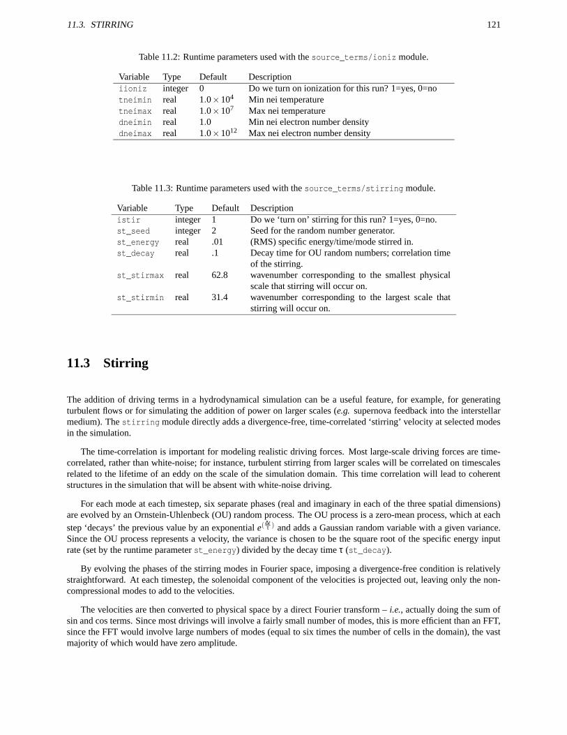
11.3. STIRRING 121
Table 11.2: Runtime parameters used with the source_terms/ioniz module.
Variable Type Default Descriptioniioniz integer 0 Do we turn on ionization for this run? 1=yes, 0=notneimin real 1.0×10⁴ Min nei temperaturetneimax real 1.0×10⁷ Max nei temperaturedneimin real 1.0 Min nei electron number densitydneimax real 1.0×10¹² Max nei electron number density
Table 11.3: Runtime parameters used with the source_terms/stirring module.
Variable Type Default Descriptionistir integer 1 Do we ‘turn on’ stirring for this run? 1=yes, 0=no.st_seed integer 2 Seed for the random number generator.st_energy real .01 (RMS) specific energy/time/mode stirred in.st_decay real .1 Decay time for OU random numbers; correlation time
of the stirring.st_stirmax real 62.8 wavenumber corresponding to the smallest physical
scale that stirring will occur on.st_stirmin real 31.4 wavenumber corresponding to the largest scale that
stirring will occur on.
11.3 Stirring
The addition of driving terms in a hydrodynamical simulation can be a useful feature, for example, for generatingturbulent flows or for simulating the addition of power on larger scales (e.g. supernova feedback into the interstellarmedium). The stirring module directly adds a divergence-free, time-correlated ‘stirring’ velocity at selected modesin the simulation.
The time-correlation is important for modeling realistic driving forces. Most large-scale driving forces are time-correlated, rather than white-noise; for instance, turbulent stirring from larger scales will be correlated on timescalesrelated to the lifetime of an eddy on the scale of the simulation domain. This time correlation will lead to coherentstructures in the simulation that will be absent with white-noise driving.
For each mode at each timestep, six separate phases (real and imaginary in each of the three spatial dimensions)are evolved by an Ornstein-Uhlenbeck (OU) random process. The OU process is a zero-mean process, which at eachstep ‘decays’ the previous value by an exponential e( ∆t
τ ) and adds a Gaussian random variable with a given variance.Since the OU process represents a velocity, the variance is chosen to be the square root of the specific energy inputrate (set by the runtime parameter st_energy) divided by the decay time τ (st_decay).
By evolving the phases of the stirring modes in Fourier space, imposing a divergence-free condition is relativelystraightforward. At each timestep, the solenoidal component of the velocities is projected out, leaving only the non-compressional modes to add to the velocities.
The velocities are then converted to physical space by a direct Fourier transform – i.e., actually doing the sum ofsin and cos terms. Since most drivings will involve a fairly small number of modes, this is more efficient than an FFT,since the FFT would involve large numbers of modes (equal to six times the number of cells in the domain), the vastmajority of which would have zero amplitude.
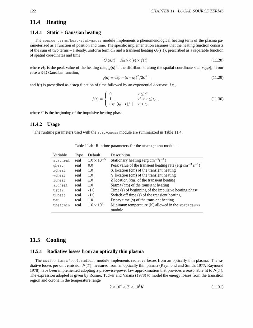
122 CHAPTER 11. LOCAL SOURCE TERMS
11.4 Heating
11.4.1 Static + Gaussian heating
The source_terms/heat/stat+gauss module implements a phenomenological heating term of the plasma pa-rameterized as a function of position and time. The specific implementation assumes that the heating function consistsof the sum of two terms – a steady, uniform term Q0 and a transient heating Qi(s, t), prescribed as a separable functionof spatial coordinates and time
Qi(s, t) = H0×g(s)× f (t) . (11.28)
where H0 is the peak value of the heating rate, g(s) is the distribution along the spatial coordinate s ≡ [x,y,z], in ourcase a 3-D Gaussian function,
g(s) = exp[−(s− s0)2/2σ2] , (11.29)
and f(t) is prescribed as a step function of time followed by an exponential decrease, i.e.,
f (t) =
0, t ≤ t∗
1, t∗ < t ≤ t0 ,exp[(t0− t)/τ], t > t0
(11.30)
where t∗ is the beginning of the impulsive heating phase.
11.4.2 Usage
The runtime parameters used with the stat+gauss module are summarized in Table 11.4.
Table 11.4: Runtime parameters for the stat+gauss module.
Variable Type Default Descriptionstatheat real 1.0×10⁻⁵ Stationary heating (erg cm−3s−1)qheat real 0.0 Peak value of the transient heating rate (erg cm−3 s−1)x0heat real 1.0 X location (cm) of the transient heatingy0heat real 1.0 Y location (cm) of the transient heatingz0heat real 1.0 Z location (cm) of the transient heatingsigheat real 1.0 Sigma (cm) of the transient heatingtstar real -1.0 Time (s) of beginning of the impulsive heating phaset0heat real -1.0 Switch off time (s) of the transient heatingtau real 1.0 Decay time (s) of the transient heatingtheatmin real 1.0×10³ Minimum temperature (K) allowed in the stat+gauss
module
11.5 Cooling
11.5.1 Radiative losses from an optically thin plasma
The source_terms/cool/radloss module implements radiative losses from an optically thin plasma. The ra-diative losses per unit emission Λ(T ) measured from an optically thin plasma (Raymond and Smith, 1977, Raymond1978) have been implemented adopting a piecewise-power law approximation that provides a reasonable fit to Λ(T ).The expression adopted is given by Rosner, Tucker and Vaiana (1978) to model the energy losses from the transitionregion and corona in the temperature range
2×10⁴ < T < 108K (11.31)
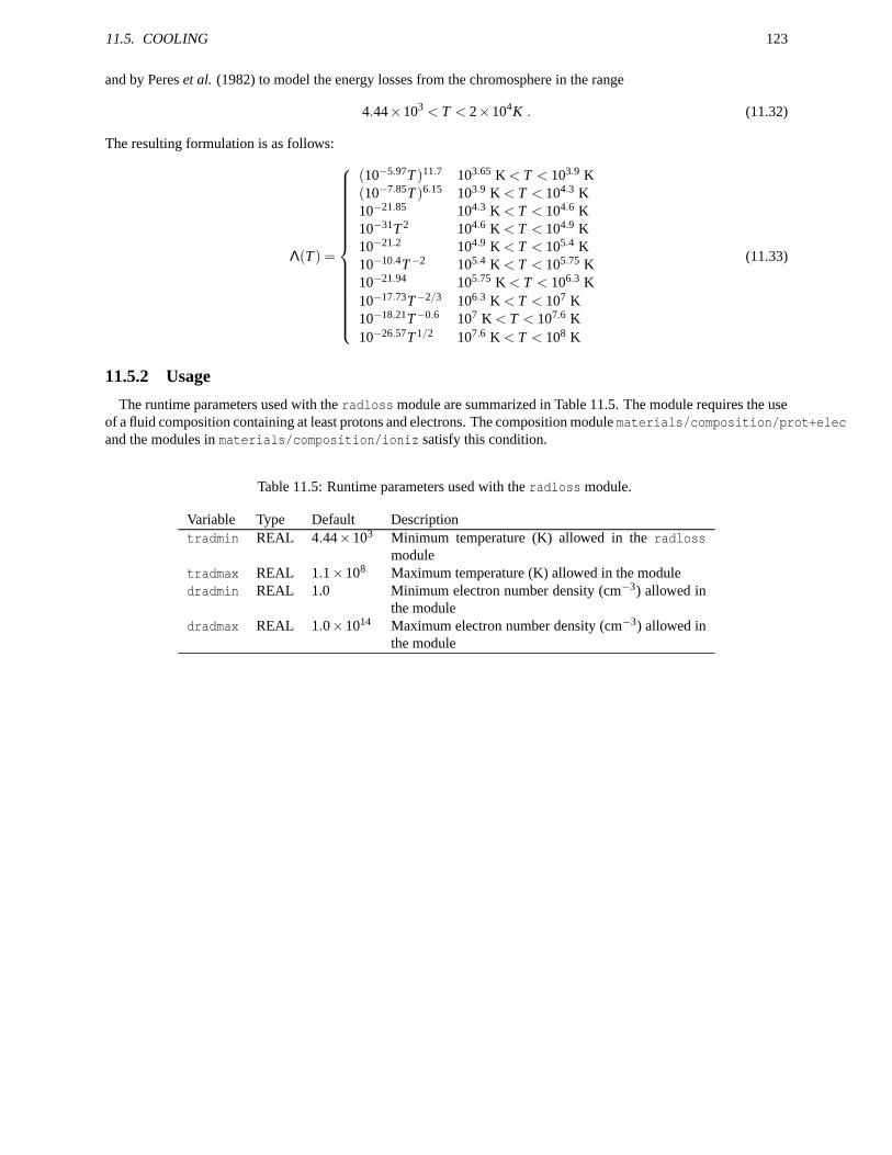
11.5. COOLING 123
and by Peres et al. (1982) to model the energy losses from the chromosphere in the range
4.44×10³ < T < 2×10⁴K . (11.32)
The resulting formulation is as follows:
Λ(T ) =
(10−5.97T )11.7 103.65 K < T < 103.9 K(10−7.85T )6.15 103.9 K < T < 104.3 K10−21.85 104.3 K < T < 104.6 K10−31T 2 104.6 K < T < 104.9 K10−21.2 104.9 K < T < 105.4 K10−10.4T−2 105.4 K < T < 105.75 K10−21.94 105.75 K < T < 106.3 K10−17.73T−2/3 106.3 K < T < 107 K10−18.21T−0.6 107 K < T < 107.6 K10−26.57T 1/2 107.6 K < T < 108 K
(11.33)
11.5.2 Usage
The runtime parameters used with the radloss module are summarized in Table 11.5. The module requires the useof a fluid composition containing at least protons and electrons. The composition module materials/composition/prot+elecand the modules in materials/composition/ioniz satisfy this condition.
Table 11.5: Runtime parameters used with the radloss module.
Variable Type Default Descriptiontradmin REAL 4.44×10³ Minimum temperature (K) allowed in the radloss
moduletradmax REAL 1.1×10⁸ Maximum temperature (K) allowed in the moduledradmin REAL 1.0 Minimum electron number density (cm−3) allowed in
the moduledradmax REAL 1.0×10¹⁴ Maximum electron number density (cm−3) allowed in
the module

124 CHAPTER 11. LOCAL SOURCE TERMS
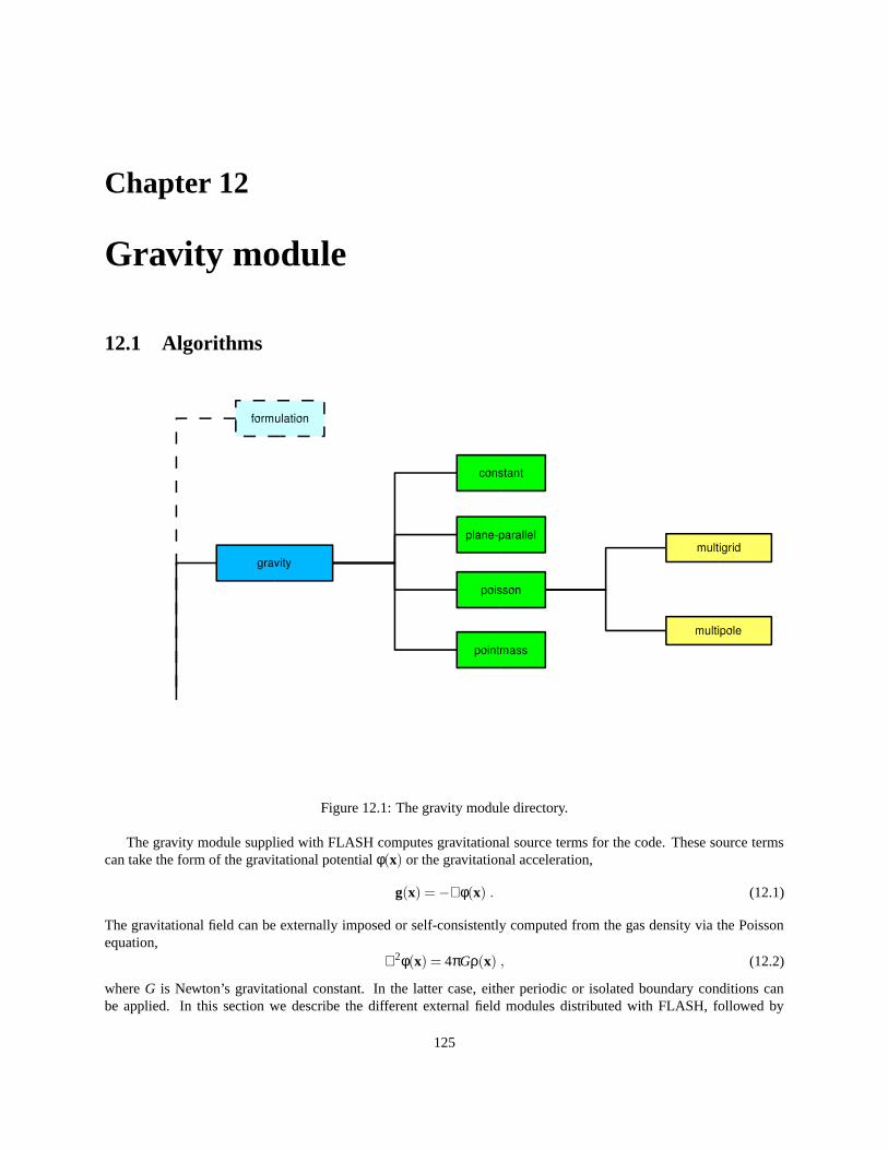
Chapter 12
Gravity module
12.1 Algorithms
Figure 12.1: The gravity module directory.
The gravity module supplied with FLASH computes gravitational source terms for the code. These source termscan take the form of the gravitational potential φ(x) or the gravitational acceleration,
g(x) =−∇φ(x) . (12.1)
The gravitational field can be externally imposed or self-consistently computed from the gas density via the Poissonequation,
∇2φ(x) = 4πGρ(x) , (12.2)
where G is Newton’s gravitational constant. In the latter case, either periodic or isolated boundary conditions canbe applied. In this section we describe the different external field modules distributed with FLASH, followed by
125
126 CHAPTER 12. GRAVITY MODULE
two algorithms for solving the Poisson equation. Coupling of gravity to other modules (e.g., hydrodynamics) is theresponsibility of those other modules, but we also discuss here the gravitational coupling method used by the PPMhydrodynamics module distributed with FLASH.
12.1.1 Externally applied fields
As distributed, FLASH includes the following externally applied gravitational fields. Each provides the accelerationvector g(x) directly, without using the gravitational potential φ(x).
1. Constant gravitational field. The gravitational acceleration is spatially constant and oriented along one of thecoordinate axes.
2. Plane-parallel gravitational field. The acceleration vector is parallel to one of the coordinate axes, and itsmagnitude drops off with distance along that axis as the inverse distance squared. Its magnitude and directionare independent of the other two coordinates.
3. Gravitational field of a point mass. The acceleration falls off with the square of the distance from a given point.The acceleration vector is everywhere directed toward this point.
12.1.2 Self-gravity algorithms
The self-gravity algorithms supplied with FLASH solve the Poisson equation (12.2) for the gravitational potentialφ(x). The modules implementing these algorithms can also return the acceleration field g(x); this is computed byfinite-differencing the potential using the expressions
gx;i jk =1
2∆x
(
φi−1, j,k−φi+1, j,k)
+O(∆x2)
gy;i jk =1
2∆y
(
φi, j−1,k−φi, j+1,k)
+O(∆y2) (12.3)
gz;i jk =1
2∆z
(
φi, j,k−1−φi, j,k+1)
+O(∆z2) .
In order to preserve the second-order accuracy of these expressions at jumps in grid refinement, it is important to usequadratic interpolants when filling guard cells at such locations. Otherwise, the truncation error of the interpolantswill produce unphysical forces at these block boundaries.
See Chapter 15 for information regarding the Poisson solvers that can be used for gravity. Currently multigrid-and multipole-based solvers are available. Each Poisson solver has a gravity sub-module interface; for example,gravity/poisson/multipole requires solvers/poisson/multipole.
12.1.2.1 Multipole Poisson solver
The multipole Poisson solver is appropriate for spherical or nearly-spherical mass distributions with isolated bound-ary conditions.
12.1.2.2 Multigrid Poisson solver
The multigrid Poisson solver is appropriate for general mass distributions and can solve problems with more generalboundary conditions. The algorithm distributed with FLASH is based on a multilevel refinement scheme described byMartin and Cartwright (1996). Isolated boundary conditions are implemented via a method based on James’ (1978)algorithm.
12.1.3 Coupling of gravity with hydrodynamics
The gravitational field couples to the Euler equations only through the momentum and energy equations. If wedefine the total energy density as
ρE ≡ 12
ρv2 +ρε , (12.4)
12.2. USING THE GRAVITY MODULES 127
where ε is the specific internal energy, then the gravitational source terms for the momentum and energy equations areρg and ρv ·g, respectively. Because of the variety of ways in which different hydrodynamics schemes treat these sourceterms, the gravity module only supplies φ and g, leaving the implementation of the fluid coupling to the hydrodynamicsmodule. Finite-difference and finite-volume hydro schemes apply the source terms in their advection steps, sometimesat multiple intermediate timesteps and sometimes using staggered meshes for vector quantities like v and g. Forexample, the PPM algorithm supplied with FLASH uses the following update steps to obtain the momentum andenergy in zone i at timestep n+1
(ρv)n+1i = (ρv)n
i +∆t2
gn+1i
(
ρni +ρn+1
i
)
(ρE)n+1i = (ρE)n
i +∆t4
gn+1i
(
ρni +ρn+1
i
)(
vni + vn+1
i
)
. (12.5)
Here gn+1i is obtained by extrapolation from φn−1
i and φni . The poisson gravity sub-module supplies a variable to
contain the potential from the previous timestep; future releases of FLASH will likely permit the storage of severaltime levels of this quantity for hydrodynamics algorithms that require more steps. Currently, g is computed at zonecenters, but this too is likely to be generalized as FLASH begins to support alternative discretization strategies. Notethat finite-volume schemes do not retain explicit conservation of momentum and energy when gravity source termsare added. Godunov schemes such as PPM, require an additional step in order to preserve second-order time accuracy.The gravitational acceleration (gn
i ) is fitted by interpolants along with the other state variables, and these interpolantsare used to construct characteristic-averaged values of g in each zone. The velocity states vL,i+1/2 and vR,i+1/2, whichare used as inputs to the Riemann problem solver, are then corrected to account for the acceleration using the followingexpressions
vL,i+1/2 → vL,i+1/2 +∆t4
(
g+L,i+1/2 +g−L,i+1/2
)
vR,i+1/2 → vR,i+1/2 +∆t4
(
g+R,i+1/2 +g−R,i+1/2
)
. (12.6)
Here g±X ,i+1/2 is the acceleration averaged using the interpolant on the X side of the interface (X = L,R) for v± ccharacteristics, which bring material to the interface between zones i and i+1 during the timestep.
12.2 Using the gravity modules
To include the effects of gravity in your FLASH executable, include the line
INCLUDE gravity/sub-module[/algorithm]
in your Modules file when you configure the code with setup. The available sub-modules include constant,planepar, poisson, and ptmass. If you are using the Poisson solver to compute the gravitational field, you mayalso specify an algorithm, currently multipole or multigrid. In this case you should also include the line
INCLUDE solvers/poisson[/algorithm]
in your Modules file. The function and usage of each of the gravity sub-modules are described in the followingsections.
Note that to use any of the gravitational field routines in your code, you must use-associate the module Gravity.Most users will be concerned only with the following routines supplied by Gravity:
• GravPotentialAllBlocks()Computes the gravitational potential on the entire mesh. For the externally imposed field sub-modules, thiscurrently does nothing. For poisson, it calls the Poisson solver using the solution variable dens as the sourceof the field. The potential is left in the solution variable gpot, and the previous contents of gpot are copied togpol.
• GravAccelAllBlocks(igpot, igrav, component)Computes the gravitational acceleration on the entire mesh. The arguments accepted are
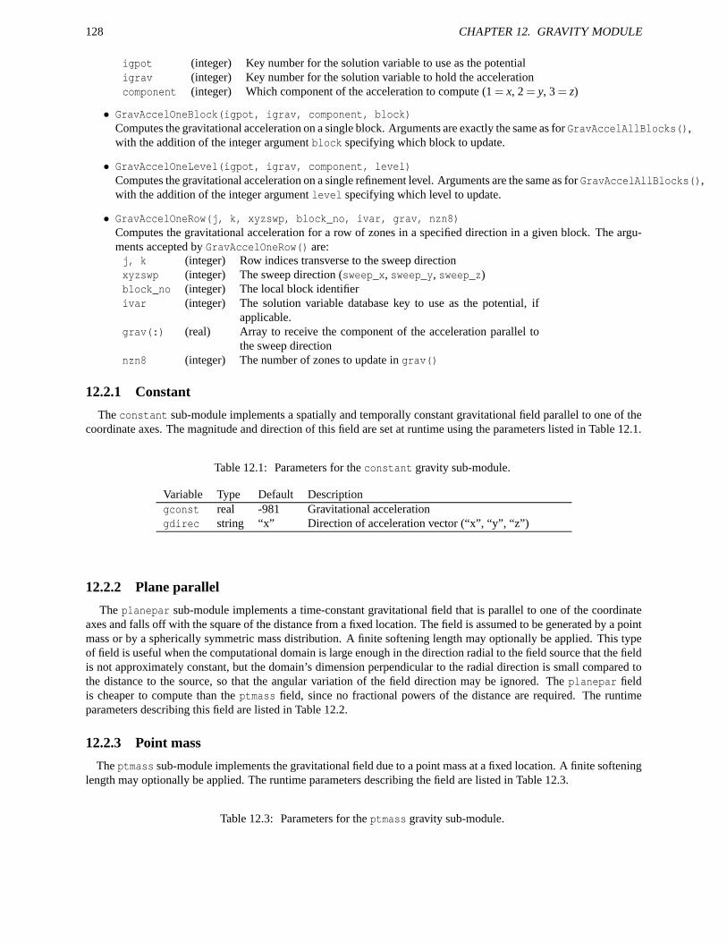
128 CHAPTER 12. GRAVITY MODULE
igpot (integer) Key number for the solution variable to use as the potentialigrav (integer) Key number for the solution variable to hold the accelerationcomponent (integer) Which component of the acceleration to compute (1 = x, 2 = y, 3 = z)
• GravAccelOneBlock(igpot, igrav, component, block)Computes the gravitational acceleration on a single block. Arguments are exactly the same as for GravAccelAllBlocks(),with the addition of the integer argument block specifying which block to update.
• GravAccelOneLevel(igpot, igrav, component, level)Computes the gravitational acceleration on a single refinement level. Arguments are the same as for GravAccelAllBlocks(),with the addition of the integer argument level specifying which level to update.
• GravAccelOneRow(j, k, xyzswp, block_no, ivar, grav, nzn8)Computes the gravitational acceleration for a row of zones in a specified direction in a given block. The argu-ments accepted by GravAccelOneRow() are:j, k (integer) Row indices transverse to the sweep directionxyzswp (integer) The sweep direction (sweep_x, sweep_y, sweep_z)block_no (integer) The local block identifierivar (integer) The solution variable database key to use as the potential, if
applicable.grav(:) (real) Array to receive the component of the acceleration parallel to
the sweep directionnzn8 (integer) The number of zones to update in grav()
12.2.1 Constant
The constant sub-module implements a spatially and temporally constant gravitational field parallel to one of thecoordinate axes. The magnitude and direction of this field are set at runtime using the parameters listed in Table 12.1.
Table 12.1: Parameters for the constant gravity sub-module.
Variable Type Default Descriptiongconst real -981 Gravitational accelerationgdirec string “x” Direction of acceleration vector (“x”, “y”, “z”)
12.2.2 Plane parallel
The planepar sub-module implements a time-constant gravitational field that is parallel to one of the coordinateaxes and falls off with the square of the distance from a fixed location. The field is assumed to be generated by a pointmass or by a spherically symmetric mass distribution. A finite softening length may optionally be applied. This typeof field is useful when the computational domain is large enough in the direction radial to the field source that the fieldis not approximately constant, but the domain’s dimension perpendicular to the radial direction is small compared tothe distance to the source, so that the angular variation of the field direction may be ignored. The planepar fieldis cheaper to compute than the ptmass field, since no fractional powers of the distance are required. The runtimeparameters describing this field are listed in Table 12.2.
12.2.3 Point mass
The ptmass sub-module implements the gravitational field due to a point mass at a fixed location. A finite softeninglength may optionally be applied. The runtime parameters describing the field are listed in Table 12.3.
Table 12.3: Parameters for the ptmass gravity sub-module.
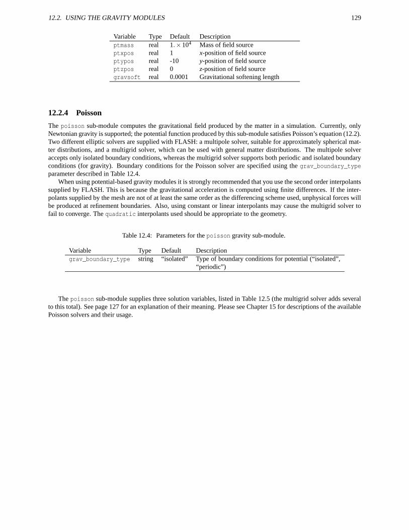
12.2. USING THE GRAVITY MODULES 129
Variable Type Default Descriptionptmass real 1.×104 Mass of field sourceptxpos real 1 x-position of field sourceptypos real -10 y-position of field sourceptzpos real 0 z-position of field sourcegravsoft real 0.0001 Gravitational softening length
12.2.4 Poisson
The poisson sub-module computes the gravitational field produced by the matter in a simulation. Currently, onlyNewtonian gravity is supported; the potential function produced by this sub-module satisfies Poisson’s equation (12.2).Two different elliptic solvers are supplied with FLASH: a multipole solver, suitable for approximately spherical mat-ter distributions, and a multigrid solver, which can be used with general matter distributions. The multipole solveraccepts only isolated boundary conditions, whereas the multigrid solver supports both periodic and isolated boundaryconditions (for gravity). Boundary conditions for the Poisson solver are specified using the grav_boundary_typeparameter described in Table 12.4.
When using potential-based gravity modules it is strongly recommended that you use the second order interpolantssupplied by FLASH. This is because the gravitational acceleration is computed using finite differences. If the inter-polants supplied by the mesh are not of at least the same order as the differencing scheme used, unphysical forces willbe produced at refinement boundaries. Also, using constant or linear interpolants may cause the multigrid solver tofail to converge. The quadratic interpolants used should be appropriate to the geometry.
Table 12.4: Parameters for the poisson gravity sub-module.
Variable Type Default Descriptiongrav_boundary_type string “isolated” Type of boundary conditions for potential (“isolated”,
“periodic”)
The poisson sub-module supplies three solution variables, listed in Table 12.5 (the multigrid solver adds severalto this total). See page 127 for an explanation of their meaning. Please see Chapter 15 for descriptions of the availablePoisson solvers and their usage.
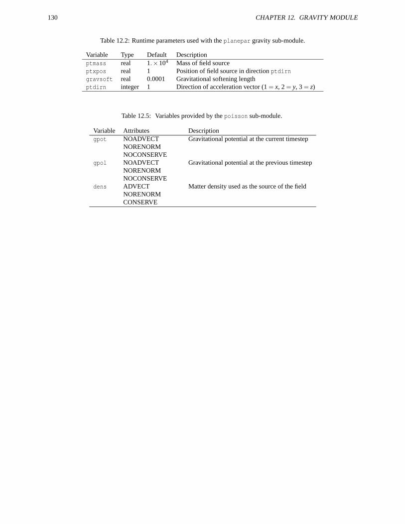
130 CHAPTER 12. GRAVITY MODULE
Table 12.2: Runtime parameters used with the planepar gravity sub-module.
Variable Type Default Descriptionptmass real 1.×104 Mass of field sourceptxpos real 1 Position of field source in direction ptdirngravsoft real 0.0001 Gravitational softening lengthptdirn integer 1 Direction of acceleration vector (1 = x, 2 = y, 3 = z)
Table 12.5: Variables provided by the poisson sub-module.
Variable Attributes Descriptiongpot NOADVECT
NORENORMNOCONSERVE
Gravitational potential at the current timestep
gpol NOADVECTNORENORMNOCONSERVE
Gravitational potential at the previous timestep
dens ADVECTNORENORMCONSERVE
Matter density used as the source of the field
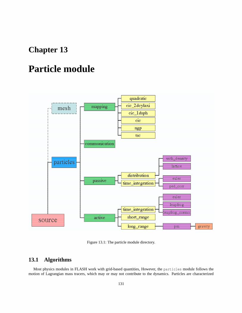
Chapter 13
Particle module
Figure 13.1: The particle module directory.
13.1 Algorithms
Most physics modules in FLASH work with grid-based quantities, However, the particles module follows themotion of Lagrangian mass tracers, which may or may not contribute to the dynamics. Particles are characterized
131
132 CHAPTER 13. PARTICLE MODULE
by positions xi, velocities vi, and sometimes other quantities such as masses mi or charges qi. Their characteristicquantities are considered to be defined at their positions and can be set by interpolation from the mesh or be used toset mesh quantities by interpolation. They move relative to the mesh and can travel from block to block, requiringcommunication patterns different from those used to transfer boundary information between processors for mesh-baseddata.
We divide particles into two types, active and passive. Active particles experience forces and may themselvescontribute to the dynamics (e.g., through long-range forces or through collisions). Solving for the motion of activeparticles is also referred to as solving the N-body problem. The equations of motion for the ith active particle are
dxi
dt= vi
midvi
dt= Flr,i +Fsr,i , (13.1)
where Flr,i represents the sum of all long-range forces (coupling all particles) acting on the ith particle and Fsr,i
represents the sum of all short-range forces (coupling only neighboring particles) acting on the particle. Passiveparticles acquire their kinematic information (velocities) directly from the mesh. They are meant to be used as passiveflow tracers and do not make sense outside of a hydrodynamical context. Since vi is externally imposed, only the firstof the above equations is relevant.
An excellent introduction to the particle techniques used in FLASH is given by R. W. Hockney and J. W. Eastwoodin Computer Simulation using Particles (IOP Publishing, 1988).
13.1.1 Active particles
Available time integration schemes for active particles include
• Forward Euler. Particles are advanced in time from tn to tn+1 = tn + ∆tn using the following difference equa-tions:
xn+1i = xn
i +vni ∆tn
vn+1i = vn
i +ani ∆tn . (13.2)
Here ai is the particle acceleration.
• Variable-timestep leapfrog. Particles are advanced using the following difference equations
x1i = x0
i +v0i ∆t0
v1/2i = v0
i +12
a0i ∆t0 (13.3)
vn+1/2i = vn−1/2
i +Cnani +Dnan−1
i
xn+1i = xn
i +vn+1/2i ∆tn .
The coefficients Cn and Dn are given by
Cn =12
∆tn +13
∆tn−1 +16
(
∆tn2
∆tn−1
)
Dn =16
(
∆tn−1− ∆tn2
∆tn−1
)
. (13.4)
By using time-centered velocities and stored accelerations, this method achieves second-order time accuracyeven with variable timesteps.
• Cosmological variable-timestep leapfrog. The coefficients in the leapfrog update are modified to take intoaccount the effect of cosmological redshift on the particles. The particle positions x are interpreted as comovingpositions, and the particle velocities v are interpreted as comoving peculiar velocities (v = x). The resultingupdate steps are
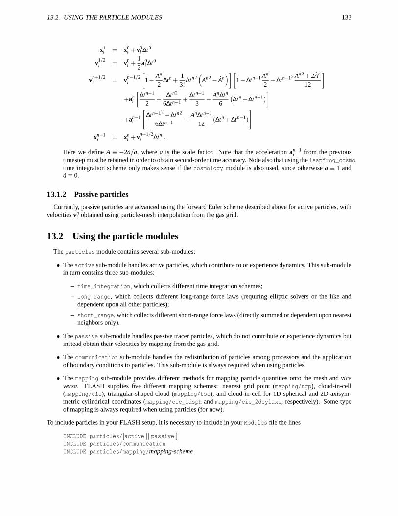
13.2. USING THE PARTICLE MODULES 133
x1i = x0
i +v0i ∆t0
v1/2i = v0
i +12
a0i ∆t0
vn+1/2i = vn−1/2
i
[
1− An
2∆tn +
13!
∆tn2(
An2− An)
][
1−∆tn−1 An
2+∆tn−12 An2 +2An
12
]
+ani
[
∆tn−1
2+
∆tn2
6∆tn−1 +∆tn−1
3− An∆tn
6
(
∆tn +∆tn−1)]
+an−1i
[
∆tn−12−∆tn2
6∆tn−1 − An∆tn−1
12(∆tn +∆tn−1)
]
xn+1i = xn
i +vn+1/2i ∆tn .
Here we define A ≡ −2a/a, where a is the scale factor. Note that the acceleration an−1i from the previous
timestep must be retained in order to obtain second-order time accuracy. Note also that using the leapfrog_cosmotime integration scheme only makes sense if the cosmology module is also used, since otherwise a ≡ 1 anda≡ 0.
13.1.2 Passive particles
Currently, passive particles are advanced using the forward Euler scheme described above for active particles, withvelocities vn
i obtained using particle-mesh interpolation from the gas grid.
13.2 Using the particle modules
The particles module contains several sub-modules:
• The active sub-module handles active particles, which contribute to or experience dynamics. This sub-modulein turn contains three sub-modules:
– time_integration, which collects different time integration schemes;
– long_range, which collects different long-range force laws (requiring elliptic solvers or the like anddependent upon all other particles);
– short_range, which collects different short-range force laws (directly summed or dependent upon nearestneighbors only).
• The passive sub-module handles passive tracer particles, which do not contribute or experience dynamics butinstead obtain their velocities by mapping from the gas grid.
• The communication sub-module handles the redistribution of particles among processors and the applicationof boundary conditions to particles. This sub-module is always required when using particles.
• The mapping sub-module provides different methods for mapping particle quantities onto the mesh and viceversa. FLASH supplies five different mapping schemes: nearest grid point (mapping/ngp), cloud-in-cell(mapping/cic), triangular-shaped cloud (mapping/tsc), and cloud-in-cell for 1D spherical and 2D axisym-metric cylindrical coordinates (mapping/cic_1dsph and mapping/cic_2dcylaxi, respectively). Some typeof mapping is always required when using particles (for now).
To include particles in your FLASH setup, it is necessary to include in your Modules file the lines
INCLUDE particles/[active || passive ]INCLUDE particles/communicationINCLUDE particles/mapping/mapping-scheme
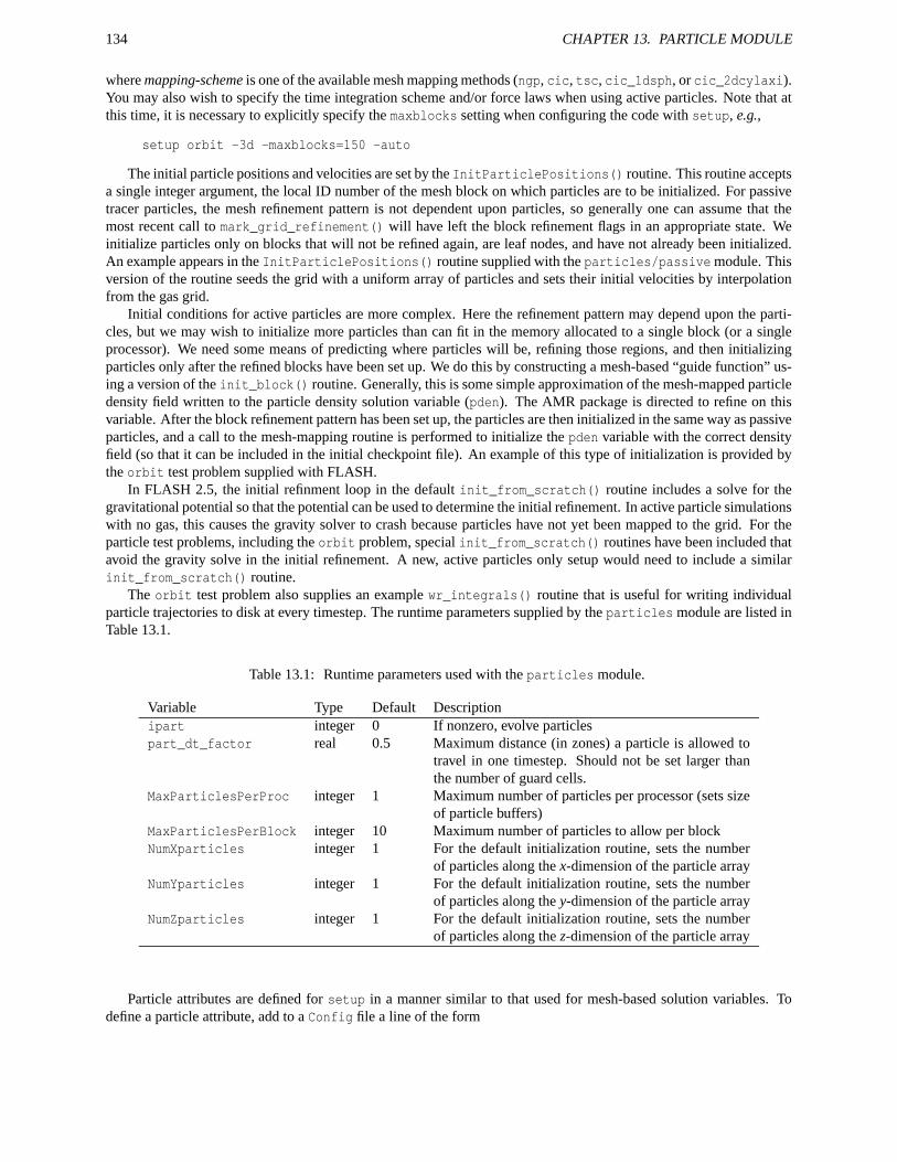
134 CHAPTER 13. PARTICLE MODULE
where mapping-scheme is one of the available mesh mapping methods (ngp, cic, tsc, cic_1dsph, or cic_2dcylaxi).You may also wish to specify the time integration scheme and/or force laws when using active particles. Note that atthis time, it is necessary to explicitly specify the maxblocks setting when configuring the code with setup, e.g.,
setup orbit -3d -maxblocks=150 -auto
The initial particle positions and velocities are set by the InitParticlePositions() routine. This routine acceptsa single integer argument, the local ID number of the mesh block on which particles are to be initialized. For passivetracer particles, the mesh refinement pattern is not dependent upon particles, so generally one can assume that themost recent call to mark_grid_refinement() will have left the block refinement flags in an appropriate state. Weinitialize particles only on blocks that will not be refined again, are leaf nodes, and have not already been initialized.An example appears in the InitParticlePositions() routine supplied with the particles/passive module. Thisversion of the routine seeds the grid with a uniform array of particles and sets their initial velocities by interpolationfrom the gas grid.
Initial conditions for active particles are more complex. Here the refinement pattern may depend upon the parti-cles, but we may wish to initialize more particles than can fit in the memory allocated to a single block (or a singleprocessor). We need some means of predicting where particles will be, refining those regions, and then initializingparticles only after the refined blocks have been set up. We do this by constructing a mesh-based “guide function” us-ing a version of the init_block() routine. Generally, this is some simple approximation of the mesh-mapped particledensity field written to the particle density solution variable (pden). The AMR package is directed to refine on thisvariable. After the block refinement pattern has been set up, the particles are then initialized in the same way as passiveparticles, and a call to the mesh-mapping routine is performed to initialize the pden variable with the correct densityfield (so that it can be included in the initial checkpoint file). An example of this type of initialization is provided bythe orbit test problem supplied with FLASH.
In FLASH 2.5, the initial refinment loop in the default init_from_scratch() routine includes a solve for thegravitational potential so that the potential can be used to determine the initial refinement. In active particle simulationswith no gas, this causes the gravity solver to crash because particles have not yet been mapped to the grid. For theparticle test problems, including the orbit problem, special init_from_scratch() routines have been included thatavoid the gravity solve in the initial refinement. A new, active particles only setup would need to include a similarinit_from_scratch() routine.
The orbit test problem also supplies an example wr_integrals() routine that is useful for writing individualparticle trajectories to disk at every timestep. The runtime parameters supplied by the particles module are listed inTable 13.1.
Table 13.1: Runtime parameters used with the particles module.
Variable Type Default Descriptionipart integer 0 If nonzero, evolve particlespart_dt_factor real 0.5 Maximum distance (in zones) a particle is allowed to
travel in one timestep. Should not be set larger thanthe number of guard cells.
MaxParticlesPerProc integer 1 Maximum number of particles per processor (sets sizeof particle buffers)
MaxParticlesPerBlock integer 10 Maximum number of particles to allow per blockNumXparticles integer 1 For the default initialization routine, sets the number
of particles along the x-dimension of the particle arrayNumYparticles integer 1 For the default initialization routine, sets the number
of particles along the y-dimension of the particle arrayNumZparticles integer 1 For the default initialization routine, sets the number
of particles along the z-dimension of the particle array
Particle attributes are defined for setup in a manner similar to that used for mesh-based solution variables. Todefine a particle attribute, add to a Config file a line of the form
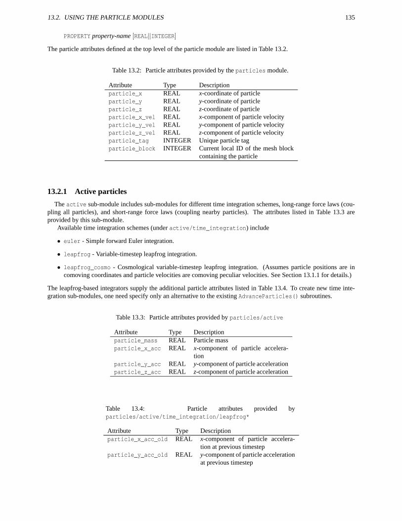
13.2. USING THE PARTICLE MODULES 135
PROPERTY property-name [REAL||INTEGER]
The particle attributes defined at the top level of the particle module are listed in Table 13.2.
Table 13.2: Particle attributes provided by the particles module.
Attribute Type Descriptionparticle_x REAL x-coordinate of particleparticle_y REAL y-coordinate of particleparticle_z REAL z-coordinate of particleparticle_x_vel REAL x-component of particle velocityparticle_y_vel REAL y-component of particle velocityparticle_z_vel REAL z-component of particle velocityparticle_tag INTEGER Unique particle tagparticle_block INTEGER Current local ID of the mesh block
containing the particle
13.2.1 Active particles
The active sub-module includes sub-modules for different time integration schemes, long-range force laws (cou-pling all particles), and short-range force laws (coupling nearby particles). The attributes listed in Table 13.3 areprovided by this sub-module.
Available time integration schemes (under active/time_integration) include
• euler - Simple forward Euler integration.
• leapfrog - Variable-timestep leapfrog integration.
• leapfrog_cosmo - Cosmological variable-timestep leapfrog integration. (Assumes particle positions are incomoving coordinates and particle velocities are comoving peculiar velocities. See Section 13.1.1 for details.)
The leapfrog-based integrators supply the additional particle attributes listed in Table 13.4. To create new time inte-gration sub-modules, one need specify only an alternative to the existing AdvanceParticles() subroutines.
Table 13.3: Particle attributes provided by particles/active
Attribute Type Descriptionparticle_mass REAL Particle massparticle_x_acc REAL x-component of particle accelera-
tionparticle_y_acc REAL y-component of particle accelerationparticle_z_acc REAL z-component of particle acceleration
Table 13.4: Particle attributes provided byparticles/active/time_integration/leapfrog*
Attribute Type Descriptionparticle_x_acc_old REAL x-component of particle accelera-
tion at previous timestepparticle_y_acc_old REAL y-component of particle acceleration
at previous timestep
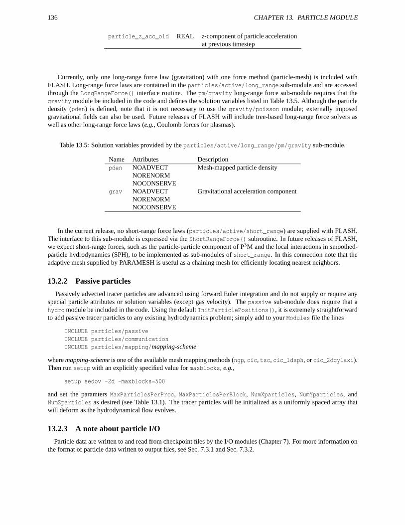
136 CHAPTER 13. PARTICLE MODULE
particle_z_acc_old REAL z-component of particle accelerationat previous timestep
Currently, only one long-range force law (gravitation) with one force method (particle-mesh) is included withFLASH. Long-range force laws are contained in the particles/active/long_range sub-module and are accessedthrough the LongRangeForce() interface routine. The pm/gravity long-range force sub-module requires that thegravity module be included in the code and defines the solution variables listed in Table 13.5. Although the particledensity (pden) is defined, note that it is not necessary to use the gravity/poisson module; externally imposedgravitational fields can also be used. Future releases of FLASH will include tree-based long-range force solvers aswell as other long-range force laws (e.g., Coulomb forces for plasmas).
Table 13.5: Solution variables provided by the particles/active/long_range/pm/gravity sub-module.
Name Attributes Descriptionpden NOADVECT
NORENORMNOCONSERVE
Mesh-mapped particle density
grav NOADVECTNORENORMNOCONSERVE
Gravitational acceleration component
In the current release, no short-range force laws (particles/active/short_range) are supplied with FLASH.The interface to this sub-module is expressed via the ShortRangeForce() subroutine. In future releases of FLASH,we expect short-range forces, such as the particle-particle component of P3M and the local interactions in smoothed-particle hydrodynamics (SPH), to be implemented as sub-modules of short_range. In this connection note that theadaptive mesh supplied by PARAMESH is useful as a chaining mesh for efficiently locating nearest neighbors.
13.2.2 Passive particles
Passively advected tracer particles are advanced using forward Euler integration and do not supply or require anyspecial particle attributes or solution variables (except gas velocity). The passive sub-module does require that ahydro module be included in the code. Using the default InitParticlePositions(), it is extremely straightforwardto add passive tracer particles to any existing hydrodynamics problem; simply add to your Modules file the lines
INCLUDE particles/passiveINCLUDE particles/communicationINCLUDE particles/mapping/mapping-scheme
where mapping-scheme is one of the available mesh mapping methods (ngp, cic, tsc, cic_1dsph, or cic_2dcylaxi).Then run setup with an explicitly specified value for maxblocks, e.g.,
setup sedov -2d -maxblocks=500
and set the paramters MaxParticlesPerProc, MaxParticlesPerBlock, NumXparticles, NumYparticles, andNumZparticles as desired (see Table 13.1). The tracer particles will be initialized as a uniformly spaced array thatwill deform as the hydrodynamical flow evolves.
13.2.3 A note about particle I/O
Particle data are written to and read from checkpoint files by the I/O modules (Chapter 7). For more information onthe format of particle data written to output files, see Sec. 7.3.1 and Sec. 7.3.2.
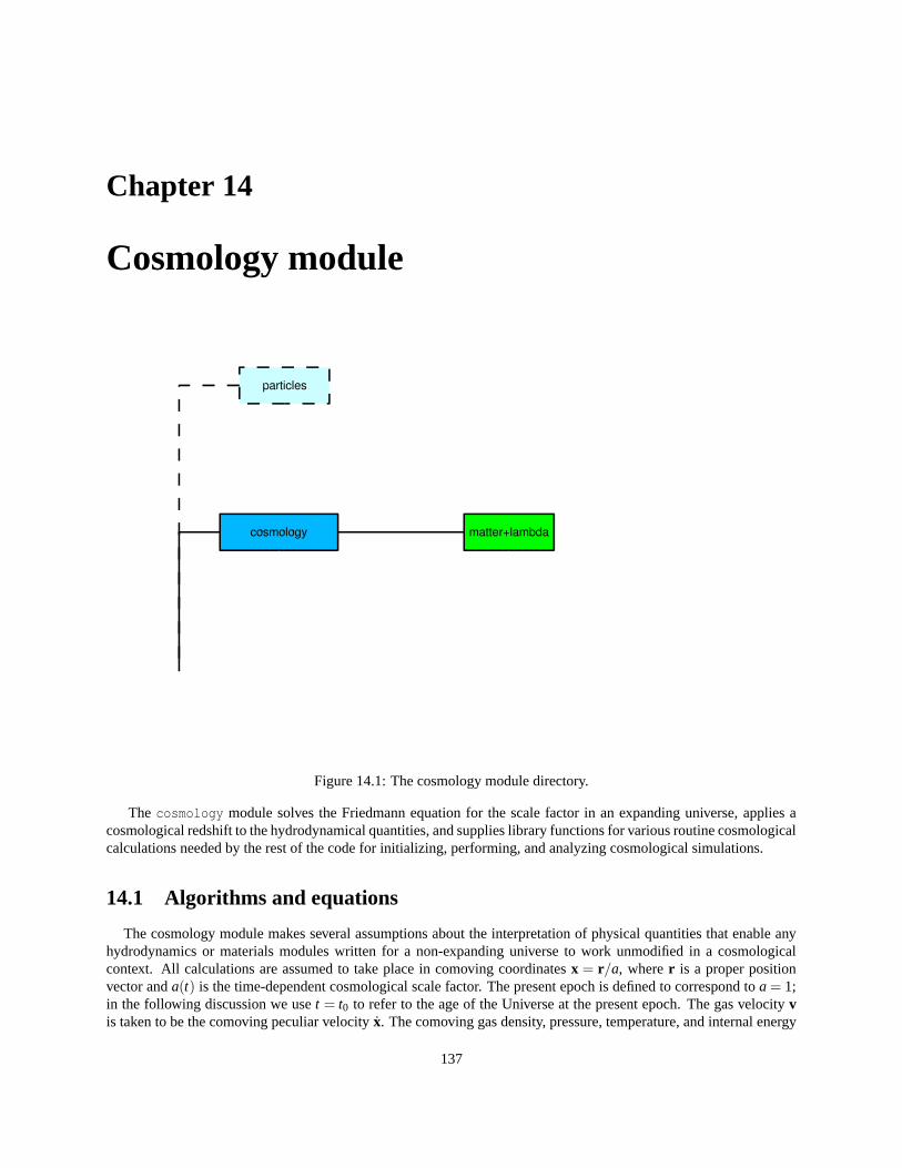
Chapter 14
Cosmology module
Figure 14.1: The cosmology module directory.
The cosmology module solves the Friedmann equation for the scale factor in an expanding universe, applies acosmological redshift to the hydrodynamical quantities, and supplies library functions for various routine cosmologicalcalculations needed by the rest of the code for initializing, performing, and analyzing cosmological simulations.
14.1 Algorithms and equations
The cosmology module makes several assumptions about the interpretation of physical quantities that enable anyhydrodynamics or materials modules written for a non-expanding universe to work unmodified in a cosmologicalcontext. All calculations are assumed to take place in comoving coordinates x = r/a, where r is a proper positionvector and a(t) is the time-dependent cosmological scale factor. The present epoch is defined to correspond to a = 1;in the following discussion we use t = t0 to refer to the age of the Universe at the present epoch. The gas velocity vis taken to be the comoving peculiar velocity x. The comoving gas density, pressure, temperature, and internal energy
137
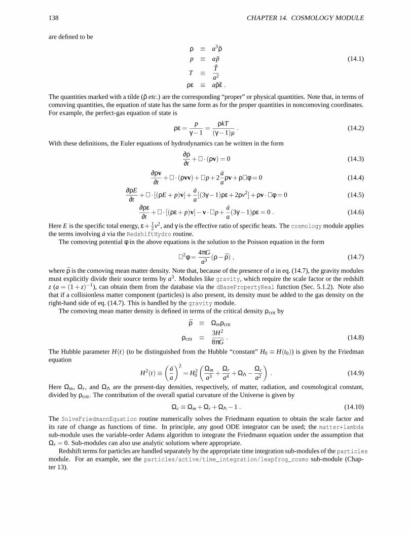
138 CHAPTER 14. COSMOLOGY MODULE
are defined to be
ρ ≡ a3ρp ≡ ap (14.1)
T ≡ Ta2
ρε ≡ aρε .
The quantities marked with a tilde (ρ etc.) are the corresponding “proper” or physical quantities. Note that, in terms ofcomoving quantities, the equation of state has the same form as for the proper quantities in noncomoving coordinates.For example, the perfect-gas equation of state is
ρε =p
γ−1=
ρkT(γ−1)µ
. (14.2)
With these definitions, the Euler equations of hydrodynamics can be written in the form
∂ρ∂t
+∇ · (ρv) = 0 (14.3)
∂ρv∂t
+∇ · (ρvv)+∇p+2aa
ρv+ρ∇φ = 0 (14.4)
∂ρE∂t
+∇ · [(ρE + p)v]+aa[(3γ−1)ρε+2ρv2]+ρv ·∇φ = 0 (14.5)
∂ρε∂t
+∇ · [(ρε+ p)v]−v ·∇p+aa(3γ−1)ρε = 0 . (14.6)
Here E is the specific total energy, ε+ 12 v2, and γ is the effective ratio of specific heats. The cosmology module applies
the terms involving a via the RedshiftHydro routine.The comoving potential φ in the above equations is the solution to the Poisson equation in the form
∇2φ =4πGa3 (ρ− ρ) , (14.7)
where ρ is the comoving mean matter density. Note that, because of the presence of a in eq. (14.7), the gravity modulesmust explicitly divide their source terms by a3. Modules like gravity, which require the scale factor or the redshiftz (a = (1 + z)−1), can obtain them from the database via the dBasePropertyReal function (Sec. 5.1.2). Note alsothat if a collisionless matter component (particles) is also present, its density must be added to the gas density on theright-hand side of eq. (14.7). This is handled by the gravity module.
The comoving mean matter density is defined in terms of the critical density ρcrit by
ρ ≡ Ωmρcrit
ρcrit ≡3H2
8πG. (14.8)
The Hubble parameter H(t) (to be distinguished from the Hubble “constant” H0 ≡ H(t0)) is given by the Friedmanequation
H2(t)≡(
aa
)2
= H20
(
Ωm
a3 +Ωr
a4 +ΩΛ−Ωc
a2
)
. (14.9)
Here Ωm, Ωr, and ΩΛ are the present-day densities, respectively, of matter, radiation, and cosmological constant,divided by ρcrit. The contribution of the overall spatial curvature of the Universe is given by
Ωc ≡Ωm +Ωr +ΩΛ−1 . (14.10)
The SolveFriedmannEquation routine numerically solves the Friedmann equation to obtain the scale factor andits rate of change as functions of time. In principle, any good ODE integrator can be used; the matter+lambdasub-module uses the variable-order Adams algorithm to integrate the Friedmann equation under the assumption thatΩr = 0. Sub-modules can also use analytic solutions where appropriate.
Redshift terms for particles are handled separately by the appropriate time integration sub-modules of the particlesmodule. For an example, see the particles/active/time_integration/leapfrog_cosmo sub-module (Chap-ter 13).
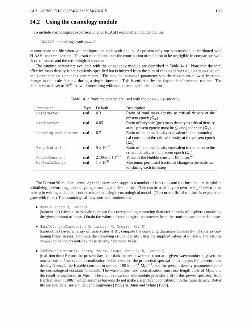
14.2. USING THE COSMOLOGY MODULE 139
14.2 Using the cosmology module
To include cosmological expansion in your FLASH executable, include the line
INCLUDE cosmology/sub-module
in your Modules file when you configure the code with setup. At present only one sub-module is distributed withFLASH: matter+lambda. This sub-module assumes the contribution of radiation to be negligible in comparison withthose of matter and the cosmological constant.
The runtime parameters available with the cosmology module are described in Table 14.1. Note that the totaleffective mass density is not explicitly specified but is inferred from the sum of the OmegaMatter, OmegaRadiation,and CosmologicalConstant parameters. The MaxScaleChange parameter sets the maximum allowed fractionalchange in the scale factor a during a single timestep. This is enforced by the ExpansionTimestep routine. Thedefault value is set to 1099 to avoid interfering with non-cosmological simulations.
Table 14.1: Runtime parameters used with the cosmology module.
Parameter Type Default DescriptionOmegaMatter real 0.3 Ratio of total mass density to critical density at the
present epoch (Ωm)OmegaBaryon real 0.05 Ratio of baryonic (gas) mass density to critical density
at the present epoch; must be ≤ OmegaMatter (Ωb)CosmologicalConstant real 0.7 Ratio of the mass density equivalent in the cosmologi-
cal constant to the critical density at the present epoch(ΩΛ)
OmegaRadiation real 5×10⁻⁵ Ratio of the mass density equivalent in radiation to thecritical density at the present epoch (Ωr)
HubbleConstant real 2.1065×10⁻¹⁸ Value of the Hubble constant H0 in sec−1
MaxScaleChange real 1×1099 Maximum permitted fractional change in the scale fac-tor during each timestep
The Fortran 90 module CosmologicalFunctions supplies a number of functions and routines that are helpful ininitializing, performing, and analyzing cosmological simulations. They can be used in your own init_block routineto help in writing code that is not restricted to a single cosmological model. (The current list of routines is expected togrow with time.) The cosmological functions and routines are:
• MassToLength(M, lambda)(subroutine) Given a mass scale M, return the corresponding comoving diameter lambda of a sphere containingthe given amount of mass. Obtain the values of cosmological parameters from the runtime parameter database.
• MassToLengthConversion(M, lambda, N, Omega0, H0, G)(subroutine) Given an array of mass scales M(N), compute the comoving diameters lambda(N) of spheres con-taining these masses. Compute the comoving critical density using the supplied values of H0 and G and assumeOmega0 to be the present-day mass density parameter value.
• CDMPowerSpectrum(k, Anorm, znorm, npspc, Omega0, h, Lambda0)(real function) Return the present-day cold dark matter power spectrum at a given wavenumber k, given thenormalization Anorm, the normalization redshift znorm, the primordial spectral index npspc, the present massdensity Omega0, the Hubble constant in units of 100 km s−1 Mpc−1, and the present density parameter due tothe cosmological constant Lambda0. The wavenumber and normalization must use length units of Mpc, andthe result is expressed in Mpc3. The matter+lambda sub-module provides a fit to this power spectrum fromBardeen et al. (1986), which assumes baryons do not make a significant contribution to the mass density. Betterfits are available; see e.g., Hu and Sugiyama (1996) or Bunn and White (1997).

140 CHAPTER 14. COSMOLOGY MODULE
• TopHatFilter(k, r)(real function) Given a wavenumber k and the characteristic length scale r (cutoff radius for the top hat filter inreal space), return the Fourier transform of the top hat filter.
• ComputeVariance(lambda, Mass, Delta0, dDelta0dM, N, f, PwrSpc, Filter, Anorm, znorm,npspc, Omega0, h, Lambda0)(subroutine) Given an array of comoving length scales lambda(N) and a processed power spectrum functionPwrSpc, compute the linear variance (δM/M)2 at the present epoch. The factor f is multiplied by the massscale in applying the smoothing kernel. Filter is a Fourier-space filter function with the same interface asTopHatFilter. Anorm, znorm, npspc, Omega0, h, and Lambda0 are passed to PwrSpc and have the same inter-pretations as in CDMPowerSpectrum. The linear variance is returned in the array Delta0(N), and its derivativewith respect to mass is returned in dDelta0dM(N). The masses corresponding to the lengths lambda are returnedin the array Mass(N).
• RedshiftToTime(z, t)(subroutine) Compute the age of the Universe t corresponding to a redshift z. Obtain the values of cosmologicalparameters from the runtime parameter database.
• RedshiftToTimeConversion(z, t, dtdz, N, Omega0, H0, Lambda0, c, Omegatot)(subroutine) Given an array of ages t(N), compute the corresponding redshifts z(N) and first derivativesdtdz(N) given a present-day mass density parameter Omega0, a Hubble constant H0, a cosmological constantdensity parameter Lambda0, the speed of light c, and the total present-day density parameter Omegatot.
• ComputeDeltaCrit(z, dcrit, dcritdz, D, N, Omega0, H0, Lambda0, Omegatot)(subroutine) Compute the linear overdensity at turnaround in the spherical collapse model at the given redshiftsz(N). dcrit(N) and dcritdz(N) return the critical overdensity and its redshift derivative, respectively. D(N)returns the growth factor for linear perturbations at the given redshifts. The remaining arguments are interpretedas for RedshiftToTimeConversion. For more details, see the appendix of Lacey and Cole (1993).
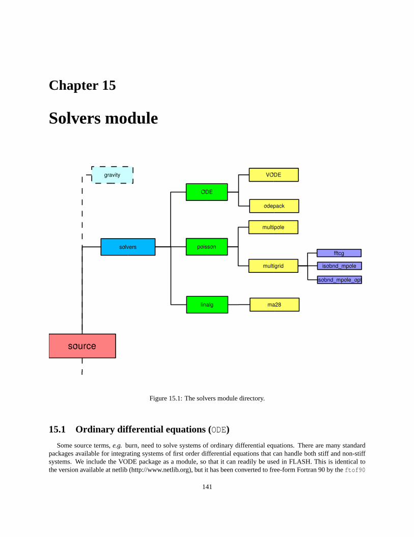
Chapter 15
Solvers module
Figure 15.1: The solvers module directory.
15.1 Ordinary differential equations (ODE)
Some source terms, e.g. burn, need to solve systems of ordinary differential equations. There are many standardpackages available for integrating systems of first order differential equations that can handle both stiff and non-stiffsystems. We include the VODE package as a module, so that it can readily be used in FLASH. This is identical tothe version available at netlib (http://www.netlib.org), but it has been converted to free-form Fortran 90 by the ftof90
141
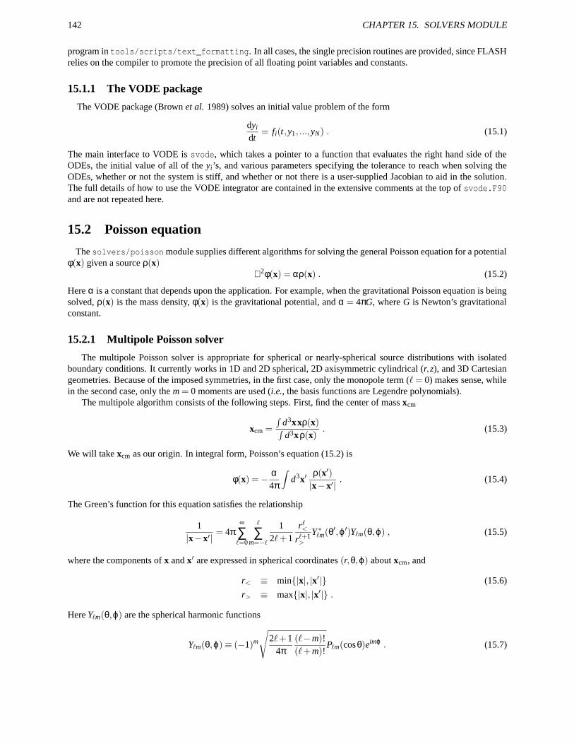
142 CHAPTER 15. SOLVERS MODULE
program in tools/scripts/text_formatting. In all cases, the single precision routines are provided, since FLASHrelies on the compiler to promote the precision of all floating point variables and constants.
15.1.1 The VODE package
The VODE package (Brown et al. 1989) solves an initial value problem of the form
dyi
dt= fi(t,y1, ...,yN) . (15.1)
The main interface to VODE is svode, which takes a pointer to a function that evaluates the right hand side of theODEs, the initial value of all of the yi’s, and various parameters specifying the tolerance to reach when solving theODEs, whether or not the system is stiff, and whether or not there is a user-supplied Jacobian to aid in the solution.The full details of how to use the VODE integrator are contained in the extensive comments at the top of svode.F90and are not repeated here.
15.2 Poisson equation
The solvers/poisson module supplies different algorithms for solving the general Poisson equation for a potentialφ(x) given a source ρ(x)
∇2φ(x) = αρ(x) . (15.2)
Here α is a constant that depends upon the application. For example, when the gravitational Poisson equation is beingsolved, ρ(x) is the mass density, φ(x) is the gravitational potential, and α = 4πG, where G is Newton’s gravitationalconstant.
15.2.1 Multipole Poisson solver
The multipole Poisson solver is appropriate for spherical or nearly-spherical source distributions with isolatedboundary conditions. It currently works in 1D and 2D spherical, 2D axisymmetric cylindrical (r,z), and 3D Cartesiangeometries. Because of the imposed symmetries, in the first case, only the monopole term (` = 0) makes sense, whilein the second case, only the m = 0 moments are used (i.e., the basis functions are Legendre polynomials).
The multipole algorithm consists of the following steps. First, find the center of mass xcm
xcm =
∫
d3xxρ(x)∫
d3xρ(x). (15.3)
We will take xcm as our origin. In integral form, Poisson’s equation (15.2) is
φ(x) =− α4π
∫
d3x′ρ(x′)|x−x′| . (15.4)
The Green’s function for this equation satisfies the relationship
1|x−x′| = 4π
∞
∑=0
`
∑m=−`
12`+1
r`<
r`+1>
Y ∗`m(θ′,ϕ′)Y`m(θ,ϕ) , (15.5)
where the components of x and x′ are expressed in spherical coordinates (r,θ,ϕ) about xcm, and
r< ≡ min|x|, |x′| (15.6)
r> ≡ max|x|, |x′| .
Here Y`m(θ,ϕ) are the spherical harmonic functions
Y`m(θ,ϕ)≡ (−1)m
√
2`+14π
(`−m)!(`+m)!
P m(cosθ)eimϕ . (15.7)
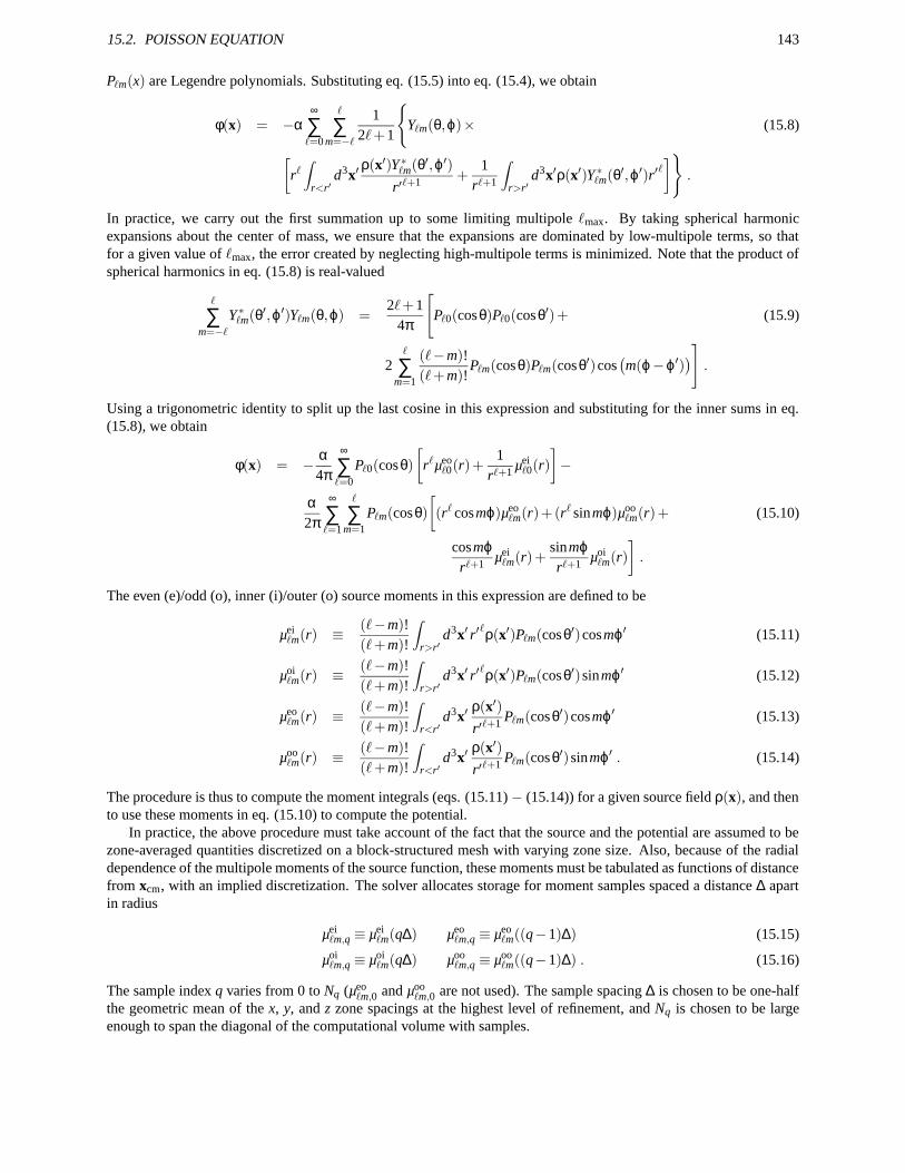
15.2. POISSON EQUATION 143
P m(x) are Legendre polynomials. Substituting eq. (15.5) into eq. (15.4), we obtain
φ(x) = −α∞
∑=0
`
∑m=−`
12`+1
Y`m(θ,ϕ)× (15.8)
[
r`∫
r<r′d3x′
ρ(x′)Y ∗`m(θ′,ϕ′)r′`+1 +
1r`+1
∫
r>r′d3x′ρ(x′)Y ∗`m(θ′,ϕ′)r′`
]
.
In practice, we carry out the first summation up to some limiting multipole `max. By taking spherical harmonicexpansions about the center of mass, we ensure that the expansions are dominated by low-multipole terms, so thatfor a given value of `max, the error created by neglecting high-multipole terms is minimized. Note that the product ofspherical harmonics in eq. (15.8) is real-valued
`
∑m=−`
Y ∗`m(θ′,ϕ′)Y`m(θ,ϕ) =2`+1
4π
[
P 0(cosθ)P 0(cosθ′)+ (15.9)
2`
∑m=1
(`−m)!(`+m)!
P m(cosθ)P m(cosθ′)cos(
m(ϕ−ϕ′))
]
.
Using a trigonometric identity to split up the last cosine in this expression and substituting for the inner sums in eq.(15.8), we obtain
φ(x) = − α4π
∞
∑=0
P 0(cosθ)
[
r`µeo`0(r)+
1r`+1 µei
`0(r)
]
−
α2π
∞
∑=1
`
∑m=1
P m(cosθ)
[
(r` cosmϕ)µeo`m(r)+(r` sinmϕ)µoo
`m(r)+ (15.10)
cosmϕr`+1 µei
`m(r)+sinmϕr`+1 µoi
`m(r)
]
.
The even (e)/odd (o), inner (i)/outer (o) source moments in this expression are defined to be
µei`m(r) ≡ (`−m)!
(`+m)!
∫
r>r′d3x′ r′`ρ(x′)P m(cosθ′)cosmϕ′ (15.11)
µoi`m(r) ≡ (`−m)!
(`+m)!
∫
r>r′d3x′ r′`ρ(x′)P m(cosθ′)sinmϕ′ (15.12)
µeo`m(r) ≡ (`−m)!
(`+m)!
∫
r<r′d3x′
ρ(x′)
r′`+1 P m(cosθ′)cosmϕ′ (15.13)
µoo`m(r) ≡ (`−m)!
(`+m)!
∫
r<r′d3x′
ρ(x′)
r′`+1 P m(cosθ′)sinmϕ′ . (15.14)
The procedure is thus to compute the moment integrals (eqs. (15.11)− (15.14)) for a given source field ρ(x), and thento use these moments in eq. (15.10) to compute the potential.
In practice, the above procedure must take account of the fact that the source and the potential are assumed to bezone-averaged quantities discretized on a block-structured mesh with varying zone size. Also, because of the radialdependence of the multipole moments of the source function, these moments must be tabulated as functions of distancefrom xcm, with an implied discretization. The solver allocates storage for moment samples spaced a distance ∆ apartin radius
µei`m,q ≡ µei
`m(q∆) µeo`m,q ≡ µeo
`m((q−1)∆) (15.15)
µoi`m,q ≡ µoi
`m(q∆) µoo`m,q ≡ µoo
`m((q−1)∆) . (15.16)
The sample index q varies from 0 to Nq (µeo`m,0 and µoo
`m,0 are not used). The sample spacing ∆ is chosen to be one-halfthe geometric mean of the x, y, and z zone spacings at the highest level of refinement, and Nq is chosen to be largeenough to span the diagonal of the computational volume with samples.
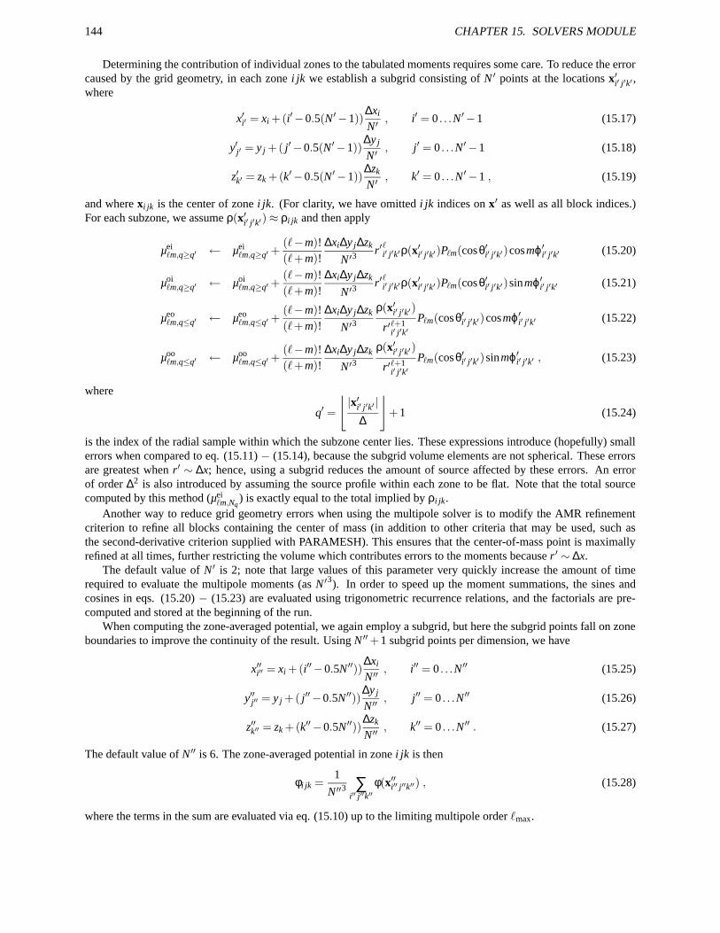
144 CHAPTER 15. SOLVERS MODULE
Determining the contribution of individual zones to the tabulated moments requires some care. To reduce the errorcaused by the grid geometry, in each zone i jk we establish a subgrid consisting of N ′ points at the locations x′i′ j′k′ ,where
x′i′ = xi +(i′−0.5(N ′−1))∆xi
N′, i′ = 0 . . .N ′−1 (15.17)
y′j′ = y j +( j′−0.5(N ′−1))∆y j
N′, j′ = 0 . . .N ′−1 (15.18)
z′k′ = zk +(k′−0.5(N ′−1))∆zk
N′, k′ = 0 . . .N ′−1 , (15.19)
and where xi jk is the center of zone i jk. (For clarity, we have omitted i jk indices on x′ as well as all block indices.)For each subzone, we assume ρ(x′i′ j′k′)≈ ρi jk and then apply
µei`m,q≥q′ ← µei
`m,q≥q′ +(`−m)!(`+m)!
∆xi∆y j∆zk
N′3r′`i′ j′k′ρ(x′i′ j′k′)P m(cosθ′i′ j′k′)cosmϕ′i′ j′k′ (15.20)
µoi`m,q≥q′ ← µoi
`m,q≥q′ +(`−m)!(`+m)!
∆xi∆y j∆zk
N′3r′`i′ j′k′ρ(x′i′ j′k′)P m(cosθ′i′ j′k′)sinmϕ′i′ j′k′ (15.21)
µeo`m,q≤q′ ← µeo
`m,q≤q′ +(`−m)!(`+m)!
∆xi∆y j∆zk
N′3ρ(x′i′ j′k′)
r′`+1i′ j′k′
P m(cosθ′i′ j′k′)cosmϕ′i′ j′k′ (15.22)
µoo`m,q≤q′ ← µoo
`m,q≤q′ +(`−m)!(`+m)!
∆xi∆y j∆zk
N′3ρ(x′i′ j′k′)
r′`+1i′ j′k′
P m(cosθ′i′ j′k′)sinmϕ′i′ j′k′ , (15.23)
where
q′ =
⌊
|x′i′ j′k′ |∆
⌋
+1 (15.24)
is the index of the radial sample within which the subzone center lies. These expressions introduce (hopefully) smallerrors when compared to eq. (15.11) − (15.14), because the subgrid volume elements are not spherical. These errorsare greatest when r′ ∼ ∆x; hence, using a subgrid reduces the amount of source affected by these errors. An errorof order ∆2 is also introduced by assuming the source profile within each zone to be flat. Note that the total sourcecomputed by this method (µei
`m,Nq) is exactly equal to the total implied by ρi jk.
Another way to reduce grid geometry errors when using the multipole solver is to modify the AMR refinementcriterion to refine all blocks containing the center of mass (in addition to other criteria that may be used, such asthe second-derivative criterion supplied with PARAMESH). This ensures that the center-of-mass point is maximallyrefined at all times, further restricting the volume which contributes errors to the moments because r ′ ∼ ∆x.
The default value of N ′ is 2; note that large values of this parameter very quickly increase the amount of timerequired to evaluate the multipole moments (as N ′3). In order to speed up the moment summations, the sines andcosines in eqs. (15.20) − (15.23) are evaluated using trigonometric recurrence relations, and the factorials are pre-computed and stored at the beginning of the run.
When computing the zone-averaged potential, we again employ a subgrid, but here the subgrid points fall on zoneboundaries to improve the continuity of the result. Using N ′′+1 subgrid points per dimension, we have
x′′i′′ = xi +(i′′−0.5N ′′))∆xi
N′′, i′′ = 0 . . .N ′′ (15.25)
y′′j′′ = y j +( j′′−0.5N ′′))∆y j
N′′, j′′ = 0 . . .N ′′ (15.26)
z′′k′′ = zk +(k′′−0.5N ′′))∆zk
N′′, k′′ = 0 . . .N ′′ . (15.27)
The default value of N ′′ is 6. The zone-averaged potential in zone i jk is then
φi jk =1
N′′3∑
i′′ j′′k′′φ(x′′i′′ j′′k′′) , (15.28)
where the terms in the sum are evaluated via eq. (15.10) up to the limiting multipole order `max.
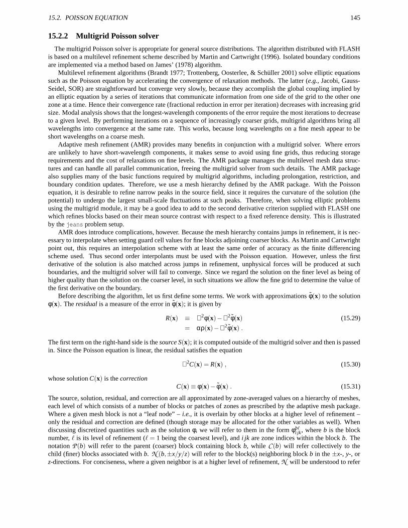
15.2. POISSON EQUATION 145
15.2.2 Multigrid Poisson solver
The multigrid Poisson solver is appropriate for general source distributions. The algorithm distributed with FLASHis based on a multilevel refinement scheme described by Martin and Cartwright (1996). Isolated boundary conditionsare implemented via a method based on James’ (1978) algorithm.
Multilevel refinement algorithms (Brandt 1977; Trottenberg, Oosterlee, & Schüller 2001) solve elliptic equationssuch as the Poisson equation by accelerating the convergence of relaxation methods. The latter (e.g., Jacobi, Gauss-Seidel, SOR) are straightforward but converge very slowly, because they accomplish the global coupling implied byan elliptic equation by a series of iterations that communicate information from one side of the grid to the other onezone at a time. Hence their convergence rate (fractional reduction in error per iteration) decreases with increasing gridsize. Modal analysis shows that the longest-wavelength components of the error require the most iterations to decreaseto a given level. By performing iterations on a sequence of increasingly coarser grids, multigrid algorithms bring allwavelengths into convergence at the same rate. This works, because long wavelengths on a fine mesh appear to beshort wavelengths on a coarse mesh.
Adaptive mesh refinement (AMR) provides many benefits in conjunction with a multigrid solver. Where errorsare unlikely to have short-wavelength components, it makes sense to avoid using fine grids, thus reducing storagerequirements and the cost of relaxations on fine levels. The AMR package manages the multilevel mesh data struc-tures and can handle all parallel communication, freeing the multigrid solver from such details. The AMR packagealso supplies many of the basic functions required by multigrid algorithms, including prolongation, restriction, andboundary condition updates. Therefore, we use a mesh hierarchy defined by the AMR package. With the Poissonequation, it is desirable to refine narrow peaks in the source field, since it requires the curvature of the solution (thepotential) to undergo the largest small-scale fluctuations at such peaks. Therefore, when solving elliptic problemsusing the multigrid module, it may be a good idea to add to the second derivative criterion supplied with FLASH onewhich refines blocks based on their mean source contrast with respect to a fixed reference density. This is illustratedby the jeans problem setup.
AMR does introduce complications, however. Because the mesh hierarchy contains jumps in refinement, it is nec-essary to interpolate when setting guard cell values for fine blocks adjoining coarser blocks. As Martin and Cartwrightpoint out, this requires an interpolation scheme with at least the same order of accuracy as the finite differencingscheme used. Thus second order interpolants must be used with the Poisson equation. However, unless the firstderivative of the solution is also matched across jumps in refinement, unphysical forces will be produced at suchboundaries, and the multigrid solver will fail to converge. Since we regard the solution on the finer level as being ofhigher quality than the solution on the coarser level, in such situations we allow the fine grid to determine the value ofthe first derivative on the boundary.
Before describing the algorithm, let us first define some terms. We work with approximations φ(x) to the solutionφ(x). The residual is a measure of the error in φ(x); it is given by
R(x) ≡ ∇2φ(x)−∇2φ(x) (15.29)
= αρ(x)−∇2φ(x) .
The first term on the right-hand side is the source S(x); it is computed outside of the multigrid solver and then is passedin. Since the Poisson equation is linear, the residual satisfies the equation
∇2C(x) = R(x) , (15.30)
whose solution C(x) is the correctionC(x)≡ φ(x)− φ(x) . (15.31)
The source, solution, residual, and correction are all approximated by zone-averaged values on a hierarchy of meshes,each level of which consists of a number of blocks or patches of zones as prescribed by the adaptive mesh package.Where a given mesh block is not a “leaf node” – i.e., it is overlain by other blocks at a higher level of refinement –only the residual and correction are defined (though storage may be allocated for the other variables as well). Whendiscussing discretized quantities such as the solution φ, we will refer to them in the form φb`
i jk, where b is the blocknumber, ` is its level of refinement (` = 1 being the coarsest level), and i jk are zone indices within the block b. Thenotation P (b) will refer to the parent (coarser) block containing block b, while C (b) will refer collectively to thechild (finer) blocks associated with b. N (b,±x/y/z) will refer to the block(s) neighboring block b in the ±x-, y-, orz-directions. For conciseness, where a given neighbor is at a higher level of refinement, N will be understood to refer

146 CHAPTER 15. SOLVERS MODULE
collectively to all of the neighboring blocks in that direction, with zone indices running from one to the product of therefinement factor with the size of block b in each dimension. Zone indices are assumed to run between 1 . . .nx, 1 . . .ny,and 1 . . .nz in each block, with a factor of 2 refinement between levels. The generalization to different block/patchsizes and different refinement factors should be fairly straightforward.
Difference operators approximating ∇2 on each grid level are defined for relaxation and for computing the residual.On level `, which has zone spacings ∆x`, ∆y`, and ∆z` in the x-, y-, and z-directions, we use
D2` φb`
i jk ≡ 1∆x`
(
D1x` φb`
i+1/2, j,k−D1x` φb`
i−1/2, j,k
)
+ (15.32)
1∆y`
(
D1y` φb`
i, j+1/2,k−D1y` φb`
i, j−1/2,k
)
+ (15.33)
1∆z`
(
D1z` φb`
i, j,k+1/2−D1z` φb`
i, j,k−1/2
)
, (15.34)
where
D1x` φb`
i+1/2, jk ≡ 1∆x`
(
φb`i+1, j,k−φb`
i, j,k
)
(15.35)
D1y` φb`
i, j+1/2,k ≡ 1∆y`
(
φb`i, j+1,k−φb`
i, j,k
)
(15.36)
D1z` φb`
i j,k+1/2 ≡ 1∆z`
(
φb`i, j,k+1−φb`
i, j,k
)
. (15.37)
In cases in which the required values of φ lie outside of a block, they are obtained from guard cells that are filledby the AMR package, possibly through restriction or prolongation from neighboring blocks. The derivative-matchingprocedure outlined above is applied only when computing the residual. In this case we replace the D 1 operators atjumps in refinement with the following operators
D ′1x` φb`
nx+1/2, jk ≡ R`
[
D1x`+1φN (b,+x),`+1
1/2,2 j−1,2k−1
]
(15.38)
D ′1x` φb`
1/2, jk ≡ R`
[
D1x`+1φN (b,−x),`+1
nx+1/2,2 j−1,2k−1
]
(15.39)
D ′1y` φb`
i,ny+1/2,k ≡ R`
[
D1y`+1φN (b,+y),`+1
2i−1,1/2,2k−1
]
(15.40)
D ′1y` φb`
i,1/2,k ≡ R`
[
D1y`+1φN (b,−y),`+1
2i−1,ny+1/2,2k−1
]
(15.41)
D ′1z` φb`
i j,nz+1/2 ≡ R`
[
D1z`+1φN (b,+z),`+1
2i−1,2 j−1,1/2
]
(15.42)
D ′1z` φb`
i j,1/2 ≡ R`
[
D1z`+1φN (b,−z),`+1
2i−1,2 j−1,nz+1/2
]
. (15.43)
The D ′1 operators are used only where the neighboring block is at the next higher level of refinement. In theseexpressions R` denotes the restriction operator that operates between levels ` and `+ 1. This is supplied along withthe prolongation operator I` by the AMR package. The relaxation operator is a Gauss-Seidel with Red-Black orderingiteration, while the coarse-grid solver applies the relaxation operator until convergence to within some threshold isattained.
Here are the steps in the multigrid algorithm:
1. Begin by initializing the solution, correction, and residual arrays to zero, if this is the first time the solver hasbeen called. Otherwise, use the previous solution as our initial guess.
2. Compute the residual Rb`i jk = Sb`
i jk−D2` φb`
i jk on all leaf blocks. Compute the discrete L2 norm of the residual andthe source.
3. Repeat the following steps until the ratio of the residual and source norms drops below some threshold, or untilwe have repeated some number of times.
4. Zero the correction C on the highest level of refinement, `max.
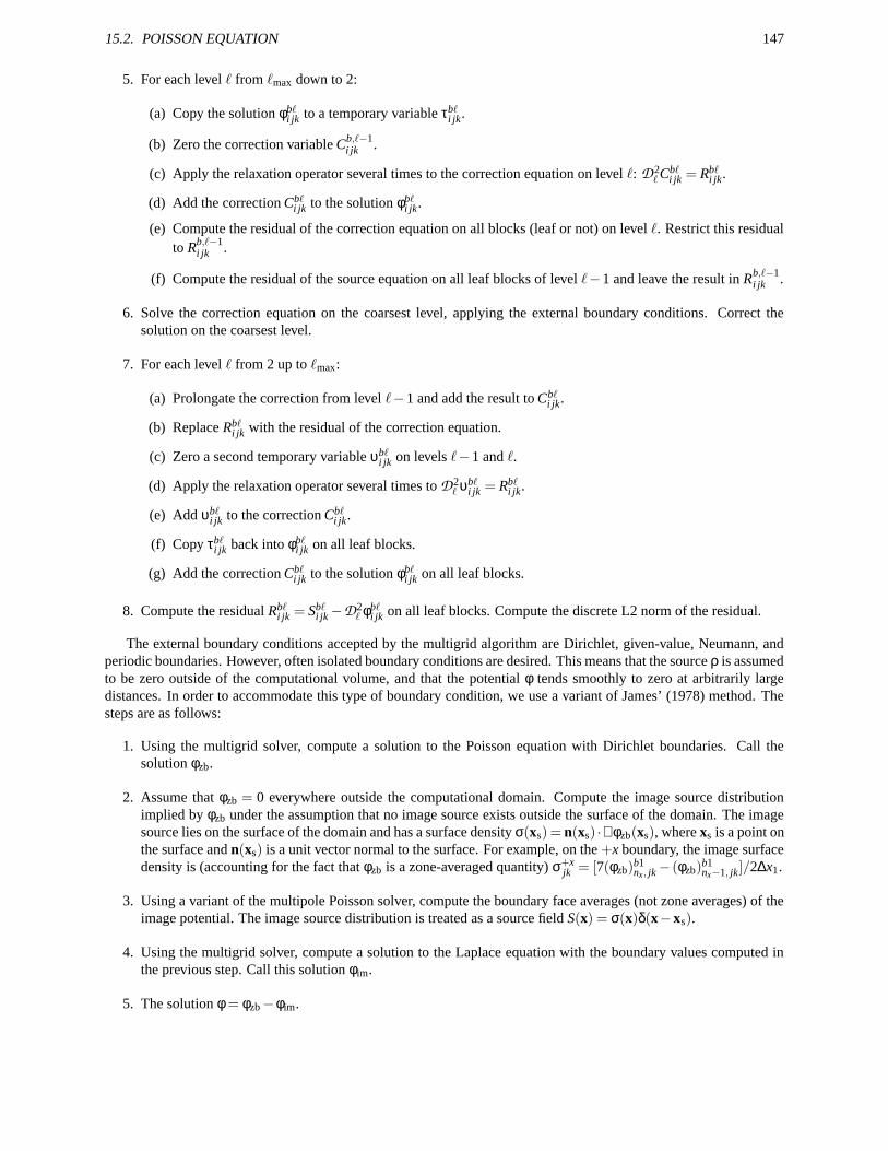
15.2. POISSON EQUATION 147
5. For each level ` from `max down to 2:
(a) Copy the solution φb`i jk to a temporary variable τb`
i jk.
(b) Zero the correction variable Cb,`−1i jk .
(c) Apply the relaxation operator several times to the correction equation on level `: D 2` Cb`
i jk = Rb`i jk.
(d) Add the correction Cb`i jk to the solution φb`
i jk.
(e) Compute the residual of the correction equation on all blocks (leaf or not) on level `. Restrict this residualto Rb,`−1
i jk .
(f) Compute the residual of the source equation on all leaf blocks of level `−1 and leave the result in Rb,`−1i jk .
6. Solve the correction equation on the coarsest level, applying the external boundary conditions. Correct thesolution on the coarsest level.
7. For each level ` from 2 up to `max:
(a) Prolongate the correction from level `−1 and add the result to Cb`i jk.
(b) Replace Rb`i jk with the residual of the correction equation.
(c) Zero a second temporary variable υb`i jk on levels `−1 and `.
(d) Apply the relaxation operator several times to D2` υb`
i jk = Rb`i jk.
(e) Add υb`i jk to the correction Cb`
i jk.
(f) Copy τb`i jk back into φb`
i jk on all leaf blocks.
(g) Add the correction Cb`i jk to the solution φb`
i jk on all leaf blocks.
8. Compute the residual Rb`i jk = Sb`
i jk−D2` φb`
i jk on all leaf blocks. Compute the discrete L2 norm of the residual.
The external boundary conditions accepted by the multigrid algorithm are Dirichlet, given-value, Neumann, andperiodic boundaries. However, often isolated boundary conditions are desired. This means that the source ρ is assumedto be zero outside of the computational volume, and that the potential φ tends smoothly to zero at arbitrarily largedistances. In order to accommodate this type of boundary condition, we use a variant of James’ (1978) method. Thesteps are as follows:
1. Using the multigrid solver, compute a solution to the Poisson equation with Dirichlet boundaries. Call thesolution φzb.
2. Assume that φzb = 0 everywhere outside the computational domain. Compute the image source distributionimplied by φzb under the assumption that no image source exists outside the surface of the domain. The imagesource lies on the surface of the domain and has a surface density σ(xs) = n(xs) ·∇φzb(xs), where xs is a point onthe surface and n(xs) is a unit vector normal to the surface. For example, on the +x boundary, the image surfacedensity is (accounting for the fact that φzb is a zone-averaged quantity) σ+x
jk = [7(φzb)b1nx, jk− (φzb)
b1nx−1, jk]/2∆x1.
3. Using a variant of the multipole Poisson solver, compute the boundary face averages (not zone averages) of theimage potential. The image source distribution is treated as a source field S(x) = σ(x)δ(x−xs).
4. Using the multigrid solver, compute a solution to the Laplace equation with the boundary values computed inthe previous step. Call this solution φim.
5. The solution φ = φzb−φim.
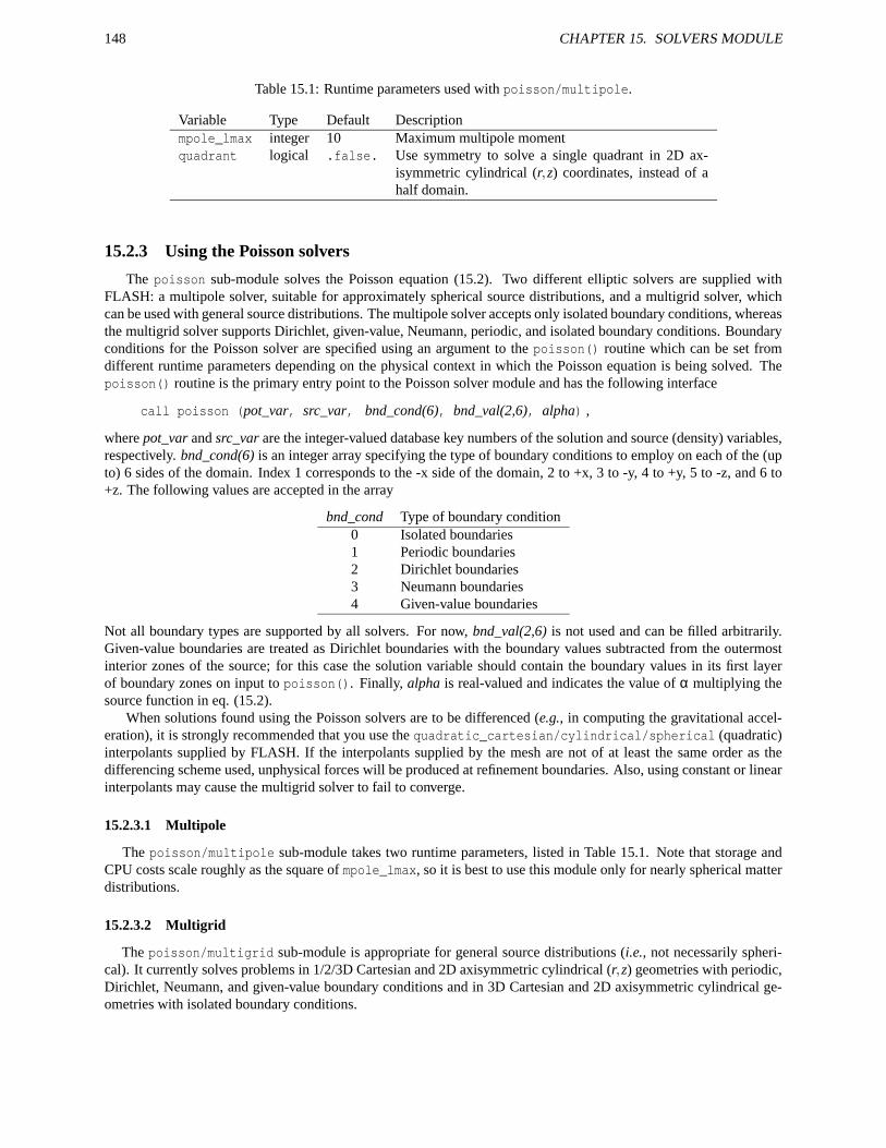
148 CHAPTER 15. SOLVERS MODULE
Table 15.1: Runtime parameters used with poisson/multipole.
Variable Type Default Descriptionmpole_lmax integer 10 Maximum multipole momentquadrant logical .false. Use symmetry to solve a single quadrant in 2D ax-
isymmetric cylindrical (r,z) coordinates, instead of ahalf domain.
15.2.3 Using the Poisson solvers
The poisson sub-module solves the Poisson equation (15.2). Two different elliptic solvers are supplied withFLASH: a multipole solver, suitable for approximately spherical source distributions, and a multigrid solver, whichcan be used with general source distributions. The multipole solver accepts only isolated boundary conditions, whereasthe multigrid solver supports Dirichlet, given-value, Neumann, periodic, and isolated boundary conditions. Boundaryconditions for the Poisson solver are specified using an argument to the poisson() routine which can be set fromdifferent runtime parameters depending on the physical context in which the Poisson equation is being solved. Thepoisson() routine is the primary entry point to the Poisson solver module and has the following interface
call poisson (pot_var, src_var, bnd_cond(6), bnd_val(2,6), alpha) ,
where pot_var and src_var are the integer-valued database key numbers of the solution and source (density) variables,respectively. bnd_cond(6) is an integer array specifying the type of boundary conditions to employ on each of the (upto) 6 sides of the domain. Index 1 corresponds to the -x side of the domain, 2 to +x, 3 to -y, 4 to +y, 5 to -z, and 6 to+z. The following values are accepted in the array
bnd_cond Type of boundary condition0 Isolated boundaries1 Periodic boundaries2 Dirichlet boundaries3 Neumann boundaries4 Given-value boundaries
Not all boundary types are supported by all solvers. For now, bnd_val(2,6) is not used and can be filled arbitrarily.Given-value boundaries are treated as Dirichlet boundaries with the boundary values subtracted from the outermostinterior zones of the source; for this case the solution variable should contain the boundary values in its first layerof boundary zones on input to poisson(). Finally, alpha is real-valued and indicates the value of α multiplying thesource function in eq. (15.2).
When solutions found using the Poisson solvers are to be differenced (e.g., in computing the gravitational accel-eration), it is strongly recommended that you use the quadratic_cartesian/cylindrical/spherical (quadratic)interpolants supplied by FLASH. If the interpolants supplied by the mesh are not of at least the same order as thedifferencing scheme used, unphysical forces will be produced at refinement boundaries. Also, using constant or linearinterpolants may cause the multigrid solver to fail to converge.
15.2.3.1 Multipole
The poisson/multipole sub-module takes two runtime parameters, listed in Table 15.1. Note that storage andCPU costs scale roughly as the square of mpole_lmax, so it is best to use this module only for nearly spherical matterdistributions.
15.2.3.2 Multigrid
The poisson/multigrid sub-module is appropriate for general source distributions (i.e., not necessarily spheri-cal). It currently solves problems in 1/2/3D Cartesian and 2D axisymmetric cylindrical (r,z) geometries with periodic,Dirichlet, Neumann, and given-value boundary conditions and in 3D Cartesian and 2D axisymmetric cylindrical ge-ometries with isolated boundary conditions.
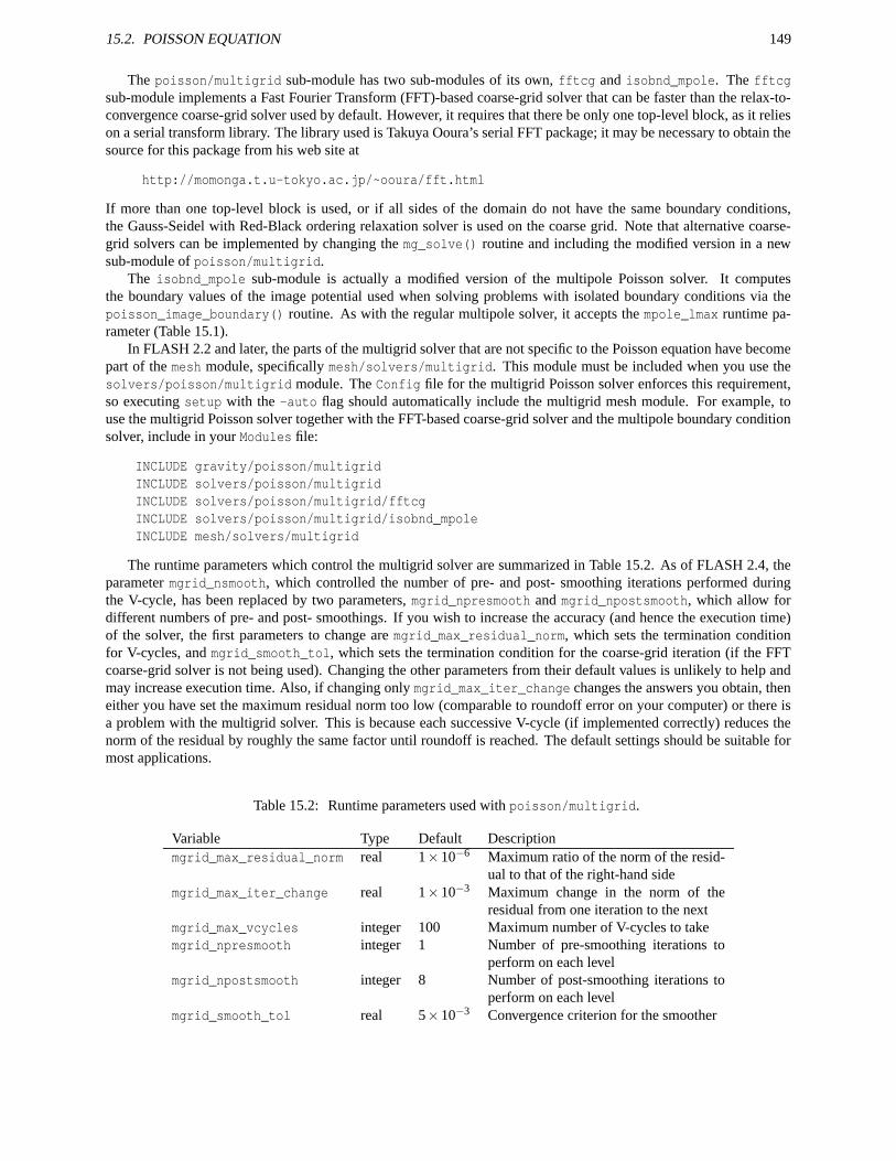
15.2. POISSON EQUATION 149
The poisson/multigrid sub-module has two sub-modules of its own, fftcg and isobnd_mpole. The fftcgsub-module implements a Fast Fourier Transform (FFT)-based coarse-grid solver that can be faster than the relax-to-convergence coarse-grid solver used by default. However, it requires that there be only one top-level block, as it relieson a serial transform library. The library used is Takuya Ooura’s serial FFT package; it may be necessary to obtain thesource for this package from his web site at
http://momonga.t.u-tokyo.ac.jp/~ooura/fft.html
If more than one top-level block is used, or if all sides of the domain do not have the same boundary conditions,the Gauss-Seidel with Red-Black ordering relaxation solver is used on the coarse grid. Note that alternative coarse-grid solvers can be implemented by changing the mg_solve() routine and including the modified version in a newsub-module of poisson/multigrid.
The isobnd_mpole sub-module is actually a modified version of the multipole Poisson solver. It computesthe boundary values of the image potential used when solving problems with isolated boundary conditions via thepoisson_image_boundary() routine. As with the regular multipole solver, it accepts the mpole_lmax runtime pa-rameter (Table 15.1).
In FLASH 2.2 and later, the parts of the multigrid solver that are not specific to the Poisson equation have becomepart of the mesh module, specifically mesh/solvers/multigrid. This module must be included when you use thesolvers/poisson/multigrid module. The Config file for the multigrid Poisson solver enforces this requirement,so executing setup with the -auto flag should automatically include the multigrid mesh module. For example, touse the multigrid Poisson solver together with the FFT-based coarse-grid solver and the multipole boundary conditionsolver, include in your Modules file:
INCLUDE gravity/poisson/multigridINCLUDE solvers/poisson/multigridINCLUDE solvers/poisson/multigrid/fftcgINCLUDE solvers/poisson/multigrid/isobnd_mpoleINCLUDE mesh/solvers/multigrid
The runtime parameters which control the multigrid solver are summarized in Table 15.2. As of FLASH 2.4, theparameter mgrid_nsmooth, which controlled the number of pre- and post- smoothing iterations performed duringthe V-cycle, has been replaced by two parameters, mgrid_npresmooth and mgrid_npostsmooth, which allow fordifferent numbers of pre- and post- smoothings. If you wish to increase the accuracy (and hence the execution time)of the solver, the first parameters to change are mgrid_max_residual_norm, which sets the termination conditionfor V-cycles, and mgrid_smooth_tol, which sets the termination condition for the coarse-grid iteration (if the FFTcoarse-grid solver is not being used). Changing the other parameters from their default values is unlikely to help andmay increase execution time. Also, if changing only mgrid_max_iter_change changes the answers you obtain, theneither you have set the maximum residual norm too low (comparable to roundoff error on your computer) or there isa problem with the multigrid solver. This is because each successive V-cycle (if implemented correctly) reduces thenorm of the residual by roughly the same factor until roundoff is reached. The default settings should be suitable formost applications.
Table 15.2: Runtime parameters used with poisson/multigrid.
Variable Type Default Descriptionmgrid_max_residual_norm real 1×10⁻⁶ Maximum ratio of the norm of the resid-
ual to that of the right-hand sidemgrid_max_iter_change real 1×10⁻³ Maximum change in the norm of the
residual from one iteration to the nextmgrid_max_vcycles integer 100 Maximum number of V-cycles to takemgrid_npresmooth integer 1 Number of pre-smoothing iterations to
perform on each levelmgrid_npostsmooth integer 8 Number of post-smoothing iterations to
perform on each levelmgrid_smooth_tol real 5×10⁻³ Convergence criterion for the smoother
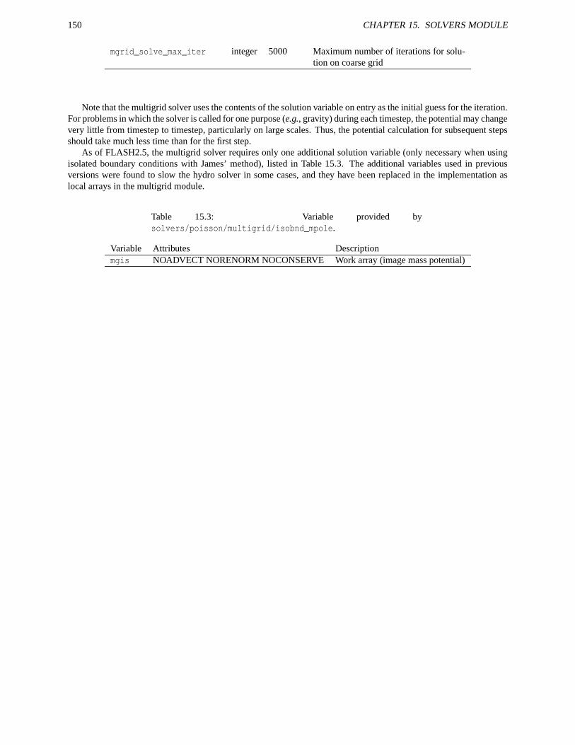
150 CHAPTER 15. SOLVERS MODULE
mgrid_solve_max_iter integer 5000 Maximum number of iterations for solu-tion on coarse grid
Note that the multigrid solver uses the contents of the solution variable on entry as the initial guess for the iteration.For problems in which the solver is called for one purpose (e.g., gravity) during each timestep, the potential may changevery little from timestep to timestep, particularly on large scales. Thus, the potential calculation for subsequent stepsshould take much less time than for the first step.
As of FLASH2.5, the multigrid solver requires only one additional solution variable (only necessary when usingisolated boundary conditions with James’ method), listed in Table 15.3. The additional variables used in previousversions were found to slow the hydro solver in some cases, and they have been replaced in the implementation aslocal arrays in the multigrid module.
Table 15.3: Variable provided bysolvers/poisson/multigrid/isobnd_mpole.
Variable Attributes Descriptionmgis NOADVECT NORENORM NOCONSERVE Work array (image mass potential)
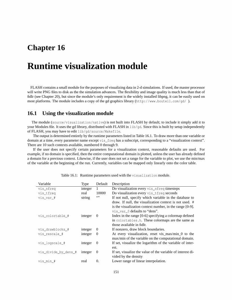
Chapter 16
Runtime visualization module
FLASH contains a small module for the purposes of visualizing data in 2-d simulations. If used, the master processorwill write PNG files to disk as the the simulation advances. The flexibility and image quality is much less than that offidlr (see Chapter 20), but since the module’s only requirement is the widely installed libpng, it can be easily used onmost platforms. The module includes a copy of the gd graphics library (http://www.boutell.com/gd/ ).
16.1 Using the visualization module
The module (source/visualization/native) is not built into FLASH by default; to include it simply add it toyour Modules file. It uses the gd library, distributed with FLASH in lib/gd. Since this is built by setup independentlyof FLASH, you may have to edit lib/gd/source/Makefile.
The output is determined entirely by the runtime parameters listed in Table 16.1. To draw more than one variable ordomain at a time, every parameter name except vis_freq has a subscript, corresponding to a “visualization context”.There are 10 such contexts available, numbered 0 through 9.
If the user does not specify certain parameters for a visualization context, reasonable defaults are used. Forexample, if no domain is specified, then the entire computational domain is plotted, unless the user has already defineda domain for a previous context. Likewise, if the user does not set a range for the variable to plot, we use the min/maxof the variable at the beginning of the run. Currently, variables can be mapped only linearly onto the color table.
Table 16.1: Runtime parameters used with the visualization module.
Variable Type Default Descriptionvis_nfreq integer 1 Do visualization every vis_nfreq timestepsvis_tfreq real 10000 Do visualization every vis_tfreq secondsvis_var_# string “” If not null, specify which variable in the database to
draw. If null, the visualization context is not used. #is the visualization context number, in the range [0-9].vis_var_0 defaults to “dens”.
vis_colortable_# integer 0 Index in the range [0-6] specifying a colormap definedin colortables.h. These colormaps are the same asthose available in fidlr.
vis_drawblocks_# integer 0 If nonzero, draw block boundaries.vis_rescale_# integer 0 At every visualization, reset vis_max/min_0 to the
max/min of the variable on the computational domain.vis_logscale_# integer 0 If set, visualize the logarithm of the variable of inter-
est.vis_divide_by_dens_# integer 0 If set, visualize the value of the variable of interest di-
vided by the densityvis_min_# real 0. Lower range of linear interpolation.
151
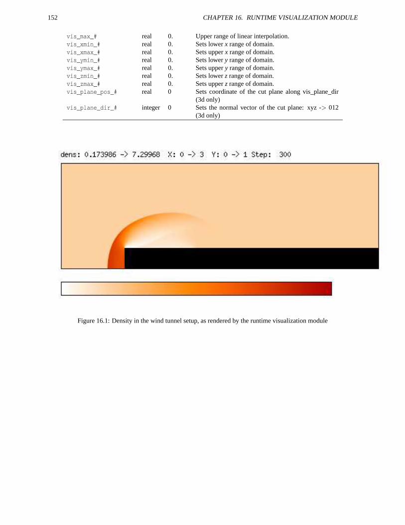
152 CHAPTER 16. RUNTIME VISUALIZATION MODULE
vis_max_# real 0. Upper range of linear interpolation.vis_xmin_# real 0. Sets lower x range of domain.vis_xmax_# real 0. Sets upper x range of domain.vis_ymin_# real 0. Sets lower y range of domain.vis_ymax_# real 0. Sets upper y range of domain.vis_zmin_# real 0. Sets lower z range of domain.vis_zmax_# real 0. Sets upper z range of domain.vis_plane_pos_# real 0 Sets coordinate of the cut plane along vis_plane_dir
(3d only)vis_plane_dir_# integer 0 Sets the normal vector of the cut plane: xyz -> 012
(3d only)
Figure 16.1: Density in the wind tunnel setup, as rendered by the runtime visualization module
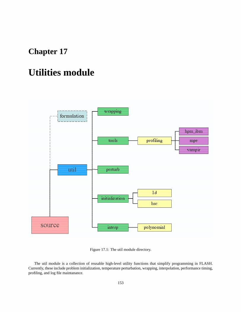
Chapter 17
Utilities module
Figure 17.1: The util module directory.
The util module is a collection of reusable high-level utility functions that simplify programming in FLASH.Currently, these include problem initialization, temperature perturbation, wrapping, interpolation, performance timing,profiling, and log file maintanance.
153
154 CHAPTER 17. UTILITIES MODULE
17.1 Initialization
There are several routines available to assist you in initializing a problem. These are intended to be used in aninit_block.F90 to read in a 1-d initial model to be mapped onto the FLASH grid. The sample_map problem (seeSec. 18.4.1) illustrates how to use the 1d initialization routine.
17.1.1 Reading one-dimensional initial models (1d)
The 1d module is a tool that reads a 1-d initial model from a file and passes it back to the caller. This model fileis required to specify the number of variables and their names in addition to the data for each point in the followingformat
# comment first -- this is my input datanumber of variables = 24denstemp..
Ni561.e-4 1.e8 1.e9 . . . .832.e-4 1.e8 1.1e9 . . . .82...
The first line of this file is a comment and is ignored by the reader. The second line specifies the number of variablescontained in the input file—this does not have to equal the number of variables in FLASH. Next, we list the variablenames, one per line, using the same names that FLASH recognizes (i.e. any of the names that appear in VARIABLElines in the Config files). When the model is read in, these names are compared to the names of the variables thatFLASH understands. Any variables contained in FLASH that are absent from the input file will be initialized to 0 (awarning will be printed to stdout). Any variables contained in the input file that are not defined in FLASH will beignored.
The variables can appear in any order in the input file. init_1d will use the order of the variable name lines todetermine which variable is which. After the variable name lines comes the data. Each line represents one point in theinitial model. The spatial coordinate is given in the first column, followed by the variables in the same order as theirdeclaration above. The initial model will be read until an EOF is encountered.
The data is passed through the argument list to the caller
integer, parameter :: n1d_max = 16384integer :: n1d_modelreal :: xzn(n1d_max), model_1d(n1d_max,nvar)
call init_1d(n1d_max, n1d_model, xzn, model_1d)
n1d_max is the maximum number of points in the initial model that you’ve allocated space for. If the initial modelcontains more points than this, an error will result, and FLASH will abort. n1d_model is the actual number of pointsread in and is returned to the caller.
The data is returned through xzn and model_1d. xzn(i) contains the coordinate of point i in the initial model.model_1d(i,j) contains the value of variable j for point i in the initial model. The variables are mapped from theorder that they are stored in the initial model file to the order that they are stored in the data structures in FLASH.Therefore, we can use dBaseKeyNumber to access a particular variable from the model file. For example, provideddensity is defined in FLASH,
idens = dBaseKeyNumber(’dens’)zone_dens = model_1d(i, idens)
stores the density in point i of the initial model in zone_dens. This allows you to initialize the solution variable inyour init_block from your initial model. See the sample_map problem for examples.
17.2. INTRODUCING TEMPERATURE PERTURBATIONS (PERTURB) 155
17.1.2 Reading hydrostatic 1D initial models (hse)
The hse initialization routine is a variant of 1d. It has basically the same job—read in an initial model and returnthe data to the caller in a manner consistent with the data layout of FLASH. The difference is that hse will restorehydrostatic equilibrium to the initial model before returning the data to the caller. This will only work with the constantgravity modules (basically anything that provides a GravAccelOneZone function).
The data is read in as above and mapped to the same ordering as FLASH. Once the file is read in, we interpolateit onto a new grid whose zone spacing is equivalent to the finest FLASH zone. This is important, since it eliminateserrors from mapping the new, HSE 1-d model onto a grid. If subsample_factor is set, then we map onto a grid that issubsample_factor times larger than the finest uniform grid. This is useful for averaging the result onto the FLASHgrid to better approximate cell averaged quantities.
Next we tweak the structure of the density to yield a model that is in HSE on this grid with the EOS used byFLASH. There are several ways we can force the model into HSE. Remember that, since PPM is a finite volumescheme and thus carries around cell averaged quantities, the unknowns are not associated with a particular point inthe zone. One point in the initial model needs to be defined as the reference point—we take its density, temperature,and composition as correct and use it as the basis for putting the other points into HSE. If reference_zone is set to’base’, then the bottommost zone is the reference. If it is set to ’fuel’, then we use the bottom-most point of the fuellayer as the reference zone. The fuel layer is defined by the point where the composition specified by fuel_markerfirst goes above the value fuel_threshold.
The density structure is adjusted by integrating the equation of hydrostatic equilibrium outward from this referencepoint. A second-order method
〈P〉+1−〈P〉0 =gδ2
(
〈ρ〉+1 + 〈ρ〉0)
, (17.1)
is used if hse_method = 1. A third-order differencing
〈P〉+1−〈P〉0 =gδ12
(
5〈ρ〉+1 +8〈ρ〉0−〈ρ〉−1
)
. (17.2)
is used if hse_method = 4. Here, δ is the mesh spacing. Derivations and further explanations of this procedure iscontained in Zingale et al. (2002).
17.2 Introducing temperature perturbations (perturb)
The perturb module allows the user to put a temperature perturbation on the grid to initiate nuclear burning. Theperturbation can be done at either constant density or isobarically and in several different shapes (currently Gaussian,tophat, and truncated Gaussian perturbations are supported).
The general usage of the perturb module is
use perturbLib
call perturbTemp(xctr, yctr, zctr, radius_x, radius_y, radius_z, &temp_perturb, pert_shape, &pert_type, block_no)
where xctr, yctr, and zctr are the coordinates of the center of the perturbation. radius_x, radius_y, and radius_zare the radius of the perturbation in each coordinate direction—allowing you to create a sphere (all lengths equal)or a generalized ellipsoid. The perturbation temperature is specified by temp_perturb and is shaped according topert_shape, which can be set equal to any one of the following
• gaussianPert
T = Tperturb exp−[(x/Rx)2 +(y/Ry)
2 +(z/Rz)2] (17.3)
156 CHAPTER 17. UTILITIES MODULE
• tophatPert
T =
Tperturb; if (x/Rx)2 +(y/Ry)
2 +(z/Rz)2 ≤ 1
Tambient; if (x/Rx)2 +(y/Ry)
2 +(z/Rz)2 > 1
(17.4)
• truncGaussPert
T = maxmin1.1 · exp−[(x/Rx)2 +(y/Ry)
2 +(z/Rz)2], Tperturb, Tambient (17.5)
Integer keys for these are publicly available through the module.The perturbation is done without modifying the density if perturb_type is set to tempOnly. To modify the
temperature field at a constant pressure (therefore, adjusting the density), perturb_type should be set to isobaric.
17.3 Wrapping Fortran functions to be called from C (wrapping)
The function of the wrapping module is to create the "glue" necessary to call Fortran functions and subroutines fromC. The bulk of the module is a python script named int2API.py which, given a file describing the Fortran functions tobe wrapped, generates the necessary Fortran and C code. This description file (with extension .int) has to be writtenby hand; it essentially looks like a list of C function prototypes. For a more detailed description of the syntax, see theusage message for int2API.
int2API.py is normally called by gmake at compile-time, since we’ve used pattern rules to make it look like anyother compiler. Given a foo.int file, it will create fooAPI-bridges.F90, fooAPI.c and fooAPI.h. This last headerfile is all that needs to be included by C programs in order to call the wrapped Fortran functions.
Currently, there are prototypes (and therefore a C interface) for most of the default database functions (seesource/database/amr/paramesh2.0/dBase.int) and a few of the runtime parameter accessors. For examplesof the wrapped functions in action, see the init_block.c files in the sod, shu_osher and wind tunnel setups; theyprovide exactly the same functionality as their init_block.F90 counterparts and are used as a test of int2API.py.As these wrapped functions have not been heavily tested, they may well behave strangely on some platforms, althoughthey should be sufficient for simple tasks.
17.4 Monitoring performance
FLASH includes a set of stopwatch-like timing routines for monitoring performance that use the timing functionalityprovided by MPI. To invoke these performance routines, the Modules file must include util/tools.
The performance routines start or stop a timer at the beginning or end of the routine(s) to be monitored andaccumulate performance information in dynamically assigned accounting segments. At the completion of the program,the routines write out a performance summary. We note that these routines are not recommended for use in timingvery short segments of code due to the overhead in accounting.
All of the source code for the performance monitoring can be found in the fortran module file perfmon.F90. Thelist below contains the performance routines along with a short description of each. Many of the subroutines areoverloaded to take either a module name or an integer index.
• timer_init ()
Initializes the performance accounting database. Calls system time routines to subtract out their initializationoverhead.
• timer_create (module,id)
Creates a timer and returns a unique integer index for the timer.
• timer_start(module)
Subroutine that begins monitoring code module module or module associated with index id. If module isnot associated with a previously assigned accounting segment, the routine creates one, whereas if id is not
17.5. PROFILING WITH JUMPSHOT, VAMPIR, OR IBM HPM 157
associated with one, then nothing is done. The parameter module is specified with a string (max 30 characters).Calling timer_start on the same module more than once without first calling timer_stop causes the currenttimer for that module to be reset (the accumulated time in the corresponding accounting segment is not reset).Timing modules may be nested as many times as there are slots for accounting segments (see MaxModulessetting). The routine may be called with an integer index instead of with the name of the module.
• timer_stop(module)
Stops accumulating time in the accounting segment associated with code module module. If timer_stop is calledfor a module that does not exist or for a module that is not currently being timed, nothing happens. The routinemay be called with an integer index instead of with the name of the module.
• timer_value(module)
Returns the current value of the timer for the accounting segment associated with the code module module orreferenced by index id. If timer_value is called for a module that does not exist, 0. is returned.
• timer_reset(module)
Resets the accumulated time in the accounting segment corresponding to the specified code module. The routinemay be called with an integer index instead of with the name of the module.
• timer_lookup_index(module)
Function that returns an integer index given a string module name. The integer index can be used in any ofthe overloaded timer routines. If a timer name is not found, the function returns timer_invalid. Use of thisfunction to obtain an integer index and subsequently calling the routines by that index rather than the stringname is encouraged for performance reasons.
• perf_summary (n_period)
Subroutine that writes a performance summary of all current accounting segments to the log file. Included is theaverage over n_period intervals (e.g. timesteps). The accounting database is not reinitialized. n_period are ofdefault integer type. Calling perf_summary stops all currently running timers.
Below is a very simple example of calling the performance routines.
program exampleuse perfmoninteger icall timer_initdo i = 1, 1000call timer_start (’blorg’)call blorgcall timer_stop (’blorg’)call timer_start (’gloob’)call gloobcall timer_stop (’gloob’)
enddocall perf_summary (1000)end
17.5 Profiling with Jumpshot, Vampir, or IBM HPM
FLASH can be used with several external profiling toolkits: Jumpshot and Vampir to profile communicationand IBM’s Hardware Performance Monitor (HPM) to profile hardware counters. Jumpshot is freely available fromArgonne National Laboratory as part of the MPE package in MPICH. Vampir is a commercial product installed atmany supercomputing centers.
158 CHAPTER 17. UTILITIES MODULE
Jumpshot and Vampir both log communication events as the code runs and provide tools to interactively andgraphically examine the logs. HPM gathers hardware counter data, generating reports on user-defined sections ofcode.
The FLASH performance monitoring module, perfmon, invokes profiling if a profiling library is included in thesetup. A call to timer_start starts profiling for a section of code, and a call to timer_stop ends the profiling. Theprofiling modules are: util/tools/profiling/mpe for Jumpshot, util/tools/profiling/vampir for Vampir, orutil/tools/profiling/hpm_ibm for HPM. The Makefile macros appropriate for linking the profiling libraries mustalso be defined in Makefile.h (see section 22): LIB_MPE for Jumpshot, LIB_VAMPIR for Vampir, LIB_HPM_IBM forHPM. For example, LIB_MPE = -L$(MPE_PATH)/lib -lmpe_f2cmpi -llmpe -lmpe.
17.6 Log file maintenance
FLASH supplies a Fortran 90 module called logfile to manage the FLASH log file, which contains various typesof useful information, warnings, and error messages produced by a FLASH run. User-written routines may also makeuse of this module as needed. The logfile routines enable a program to open and close a log file, write time or datestamps to the file, and write arbitrary messages to the file. The file is kept closed and is only opened for appendingwhen information is to be written, avoiding problems with unflushed buffers. For this reason, logfile routines shouldnot be called within time-sensitive loops, as the routines will generate system calls.
An example program using the logfile module might appear as follows:
program testuse logfileinteger :: icall create_logfile ("test.log", "test.par", .false.)call stamp_logfile ("beginning log file test...")do i = 1, 10call open_logfilewrite (log_lun,*) ’i = ’, icall close_logfile
enddocall stamp_logfile ("done with log file test.")end
The following routines, data types, and public constants are provided by this module.
• create_logfile (name, parmfile, restart)
Creates the named log file and writes some header information to it, including the build stamp and the values ofall runtime parameters in the global parameter context. The name of the parameter file is taken as an input; it isechoed to the log file. If restart is .true., the file is opened in append mode.
• stamp_logfile (string)
Write a date stamp and a specified string to the log file.
• tstamp_logfile (n, t, dt)
Write a dated timestep stamp for step n, time t, timestep dt to the log file. n must be an integer, while t and dtmust be reals.
• write_logfile (string)
Write a string to the log file without a date stamp.
• break_logfile()
Write a ‘break’ (a row of =) to the log file.

17.6. LOG FILE MAINTENANCE 159
• open_logfile()
Open the log file for writing, creating it first with a default name (logfile) if necessary. open_logfile() andclose_logfile() should only be used if it is necessary to write something directly to the log file unit withsome external routine.
• close_logfile()
Close the log file.
• log_lun
The logical unit number being used by the logfile module (to permit direct writes to the log file by externalroutines).

160 CHAPTER 17. UTILITIES MODULE

Part III
Test Cases
161

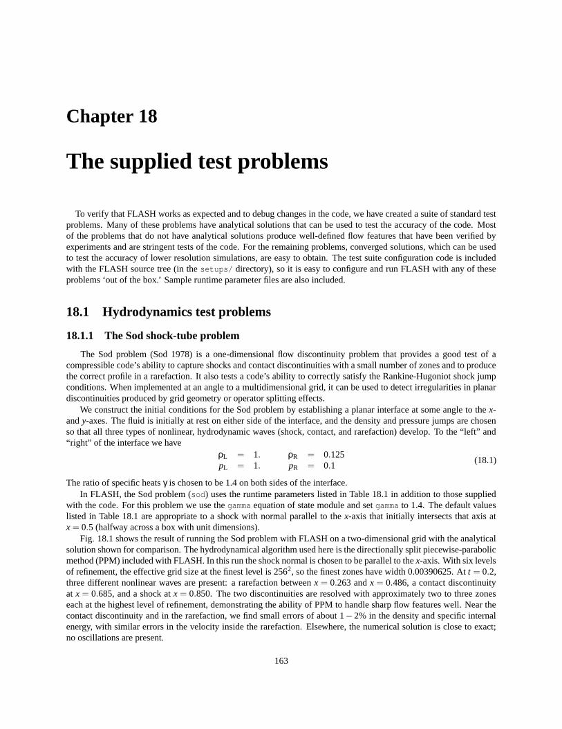
Chapter 18
The supplied test problems
To verify that FLASH works as expected and to debug changes in the code, we have created a suite of standard testproblems. Many of these problems have analytical solutions that can be used to test the accuracy of the code. Mostof the problems that do not have analytical solutions produce well-defined flow features that have been verified byexperiments and are stringent tests of the code. For the remaining problems, converged solutions, which can be usedto test the accuracy of lower resolution simulations, are easy to obtain. The test suite configuration code is includedwith the FLASH source tree (in the setups/ directory), so it is easy to configure and run FLASH with any of theseproblems ‘out of the box.’ Sample runtime parameter files are also included.
18.1 Hydrodynamics test problems
18.1.1 The Sod shock-tube problem
The Sod problem (Sod 1978) is a one-dimensional flow discontinuity problem that provides a good test of acompressible code’s ability to capture shocks and contact discontinuities with a small number of zones and to producethe correct profile in a rarefaction. It also tests a code’s ability to correctly satisfy the Rankine-Hugoniot shock jumpconditions. When implemented at an angle to a multidimensional grid, it can be used to detect irregularities in planardiscontinuities produced by grid geometry or operator splitting effects.
We construct the initial conditions for the Sod problem by establishing a planar interface at some angle to the x-and y-axes. The fluid is initially at rest on either side of the interface, and the density and pressure jumps are chosenso that all three types of nonlinear, hydrodynamic waves (shock, contact, and rarefaction) develop. To the “left” and“right” of the interface we have
ρL = 1. ρR = 0.125pL = 1. pR = 0.1
(18.1)
The ratio of specific heats γ is chosen to be 1.4 on both sides of the interface.In FLASH, the Sod problem (sod) uses the runtime parameters listed in Table 18.1 in addition to those supplied
with the code. For this problem we use the gamma equation of state module and set gamma to 1.4. The default valueslisted in Table 18.1 are appropriate to a shock with normal parallel to the x-axis that initially intersects that axis atx = 0.5 (halfway across a box with unit dimensions).
Fig. 18.1 shows the result of running the Sod problem with FLASH on a two-dimensional grid with the analyticalsolution shown for comparison. The hydrodynamical algorithm used here is the directionally split piecewise-parabolicmethod (PPM) included with FLASH. In this run the shock normal is chosen to be parallel to the x-axis. With six levelsof refinement, the effective grid size at the finest level is 2562, so the finest zones have width 0.00390625. At t = 0.2,three different nonlinear waves are present: a rarefaction between x = 0.263 and x = 0.486, a contact discontinuityat x = 0.685, and a shock at x = 0.850. The two discontinuities are resolved with approximately two to three zoneseach at the highest level of refinement, demonstrating the ability of PPM to handle sharp flow features well. Near thecontact discontinuity and in the rarefaction, we find small errors of about 1− 2% in the density and specific internalenergy, with similar errors in the velocity inside the rarefaction. Elsewhere, the numerical solution is close to exact;no oscillations are present.
163
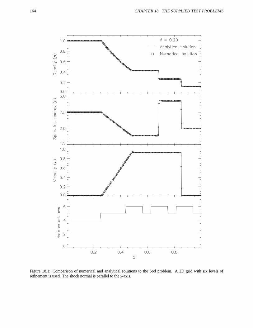
164 CHAPTER 18. THE SUPPLIED TEST PROBLEMS
Figure 18.1: Comparison of numerical and analytical solutions to the Sod problem. A 2D grid with six levels ofrefinement is used. The shock normal is parallel to the x-axis.
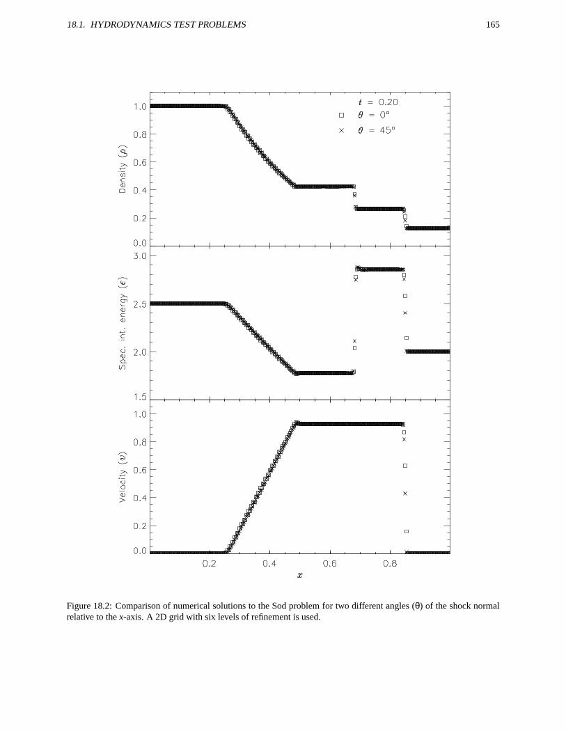
18.1. HYDRODYNAMICS TEST PROBLEMS 165
Figure 18.2: Comparison of numerical solutions to the Sod problem for two different angles (θ) of the shock normalrelative to the x-axis. A 2D grid with six levels of refinement is used.
166 CHAPTER 18. THE SUPPLIED TEST PROBLEMS
Table 18.1: Runtime parameters used with the sod test problem.
Variable Type Default Descriptionrho_left real 1 Initial density to the left of the interface (ρL)rho_right real 0.125 Initial density to the right (ρR)p_left real 1 Initial pressure to the left (pL)p_right real 0.1 Initial pressure to the right (pR)u_left real 0 Initial velocity (perpendicular to interface) to the left
(uL)u_right real 0 Initial velocity (perpendicular to interface) to the right
(uR)xangle real 0 Angle made by interface normal with the x-axis (de-
grees)yangle real 90 Angle made by interface normal with the y-axis (de-
grees)posn real 0.5 Point of intersection between the interface plane and
the x-axis
Fig. 18.2 shows the result of running the Sod problem on the same two-dimensional grid with different shocknormals: parallel to the x-axis (θ = 0) and along the box diagonal (θ = 45). For the diagonal solution, we haveinterpolated values of density, specific internal energy, and velocity to a set of 256 points spaced exactly as in thex-axis solution. This comparison shows the effects of the second-order directional splitting used with FLASH onthe resolution of shocks. At the right side of the rarefaction and at the contact discontinuity, the diagonal solutionundergoes slightly larger oscillations (on the order of a few percent) than the x-axis solution. Also, the value of eachvariable inside the discontinuity regions differs between the two solutions by up to 10%. However, the location andthickness of the discontinuities is the same for the two solutions. In general, shocks at an angle to the grid are resolvedwith approximately the same number of zones as shocks parallel to a coordinate axis.
Fig. 18.3 presents a colormap plot of the density at t = 0.2 in the diagonal solution together with the block structureof the AMR grid. Note that regions surrounding the discontinuities are maximally refined, while behind the shock andcontact discontinuity, the grid has de-refined, because the second derivative of the density has decreased in magnitude.Because zero-gradient outflow boundaries were used for this test, some reflections are present at the upper left andlower right corners, but at t = 0.2 these have not yet propagated to the center of the grid.
18.1.2 The Woodward-Colella interacting blast-wave problem
This problem was originally used by Woodward and Colella (1984) to compare the performance of several differenthydrodynamical methods on problems involving strong shocks and narrow features. It has no analytical solution(except at very early times), but since it is one-dimensional, it is easy to produce a converged solution by runningthe code with a very large number of zones, permitting an estimate of the self-convergence rate. For FLASH, it alsoprovides a good test of the adaptive mesh refinement scheme.
The initial conditions consist of two parallel, planar flow discontinuities. Reflecting boundary conditions are used.The density is unity and the velocity is zero everywhere. The pressure is large at the left and right and small in thecenter
pL = 1000, pM = 0.01, pR = 100 . (18.2)
The equation of state is that of a perfect gas with γ = 1.4.Fig. 18.4 shows the density and velocity profiles at several different times in the converged solution, demonstrating
the complexity inherent in this problem. The initial pressure discontinuities drive shocks into the middle part of thegrid; behind them, rarefactions form and propagate toward the outer boundaries, where they are reflected back into thegrid. By the time the shocks collide at t = 0.028, the reflected rarefactions have caught up to them, weakening themand making their post-shock structure more complex. Because the right-hand shock is initially weaker, the rarefactionon that side reflects from the wall later, so the resulting shock structures going into the collision from the left and rightare quite different. Behind each shock is a contact discontinuity left over from the initial conditions (at x ≈ 0.50 and
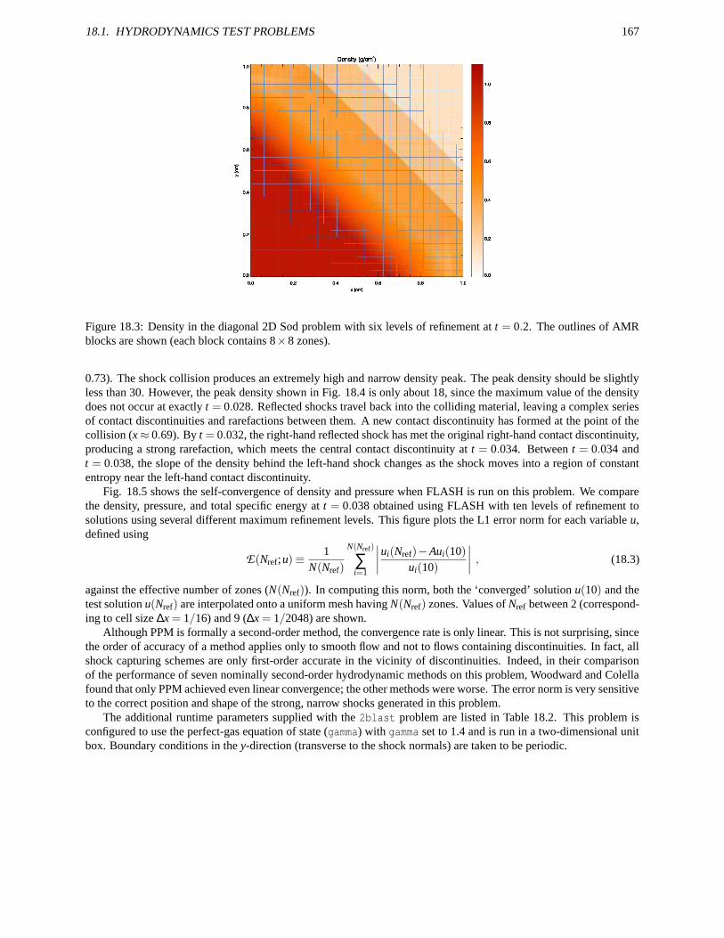
18.1. HYDRODYNAMICS TEST PROBLEMS 167
Figure 18.3: Density in the diagonal 2D Sod problem with six levels of refinement at t = 0.2. The outlines of AMRblocks are shown (each block contains 8×8 zones).
0.73). The shock collision produces an extremely high and narrow density peak. The peak density should be slightlyless than 30. However, the peak density shown in Fig. 18.4 is only about 18, since the maximum value of the densitydoes not occur at exactly t = 0.028. Reflected shocks travel back into the colliding material, leaving a complex seriesof contact discontinuities and rarefactions between them. A new contact discontinuity has formed at the point of thecollision (x≈ 0.69). By t = 0.032, the right-hand reflected shock has met the original right-hand contact discontinuity,producing a strong rarefaction, which meets the central contact discontinuity at t = 0.034. Between t = 0.034 andt = 0.038, the slope of the density behind the left-hand shock changes as the shock moves into a region of constantentropy near the left-hand contact discontinuity.
Fig. 18.5 shows the self-convergence of density and pressure when FLASH is run on this problem. We comparethe density, pressure, and total specific energy at t = 0.038 obtained using FLASH with ten levels of refinement tosolutions using several different maximum refinement levels. This figure plots the L1 error norm for each variable u,defined using
E(Nref;u)≡ 1N(Nref)
N(Nref)
∑i=1
∣
∣
∣
∣
ui(Nref)−Aui(10)
ui(10)
∣
∣
∣
∣
, (18.3)
against the effective number of zones (N(Nref)). In computing this norm, both the ‘converged’ solution u(10) and thetest solution u(Nref) are interpolated onto a uniform mesh having N(Nref) zones. Values of Nref between 2 (correspond-ing to cell size ∆x = 1/16) and 9 (∆x = 1/2048) are shown.
Although PPM is formally a second-order method, the convergence rate is only linear. This is not surprising, sincethe order of accuracy of a method applies only to smooth flow and not to flows containing discontinuities. In fact, allshock capturing schemes are only first-order accurate in the vicinity of discontinuities. Indeed, in their comparisonof the performance of seven nominally second-order hydrodynamic methods on this problem, Woodward and Colellafound that only PPM achieved even linear convergence; the other methods were worse. The error norm is very sensitiveto the correct position and shape of the strong, narrow shocks generated in this problem.
The additional runtime parameters supplied with the 2blast problem are listed in Table 18.2. This problem isconfigured to use the perfect-gas equation of state (gamma) with gamma set to 1.4 and is run in a two-dimensional unitbox. Boundary conditions in the y-direction (transverse to the shock normals) are taken to be periodic.
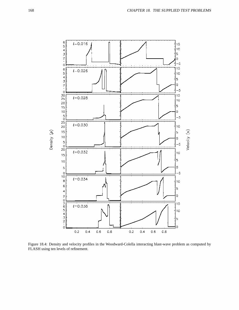
168 CHAPTER 18. THE SUPPLIED TEST PROBLEMS
Figure 18.4: Density and velocity profiles in the Woodward-Colella interacting blast-wave problem as computed byFLASH using ten levels of refinement.
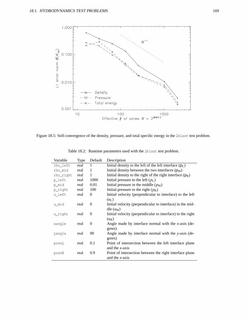
18.1. HYDRODYNAMICS TEST PROBLEMS 169
Figure 18.5: Self-convergence of the density, pressure, and total specific energy in the 2blast test problem.
Table 18.2: Runtime parameters used with the 2blast test problem.
Variable Type Default Descriptionrho_left real 1 Initial density to the left of the left interface (ρL)rho_mid real 1 Initial density between the two interfaces (ρM)rho_right real 1 Initial density to the right of the right interface (ρR)p_left real 1000 Initial pressure to the left (pL)p_mid real 0.01 Initial pressure in the middle (pM)p_right real 100 Initial pressure to the right (pR)u_left real 0 Initial velocity (perpendicular to interface) to the left
(uL)u_mid real 0 Initial velocity (perpendicular to interface) in the mid-
dle (uM)u_right real 0 Initial velocity (perpendicular to interface) to the right
(uR)xangle real 0 Angle made by interface normal with the x-axis (de-
grees)yangle real 90 Angle made by interface normal with the y-axis (de-
grees)posnL real 0.1 Point of intersection between the left interface plane
and the x-axisposnR real 0.9 Point of intersection between the right interface plane
and the x-axis
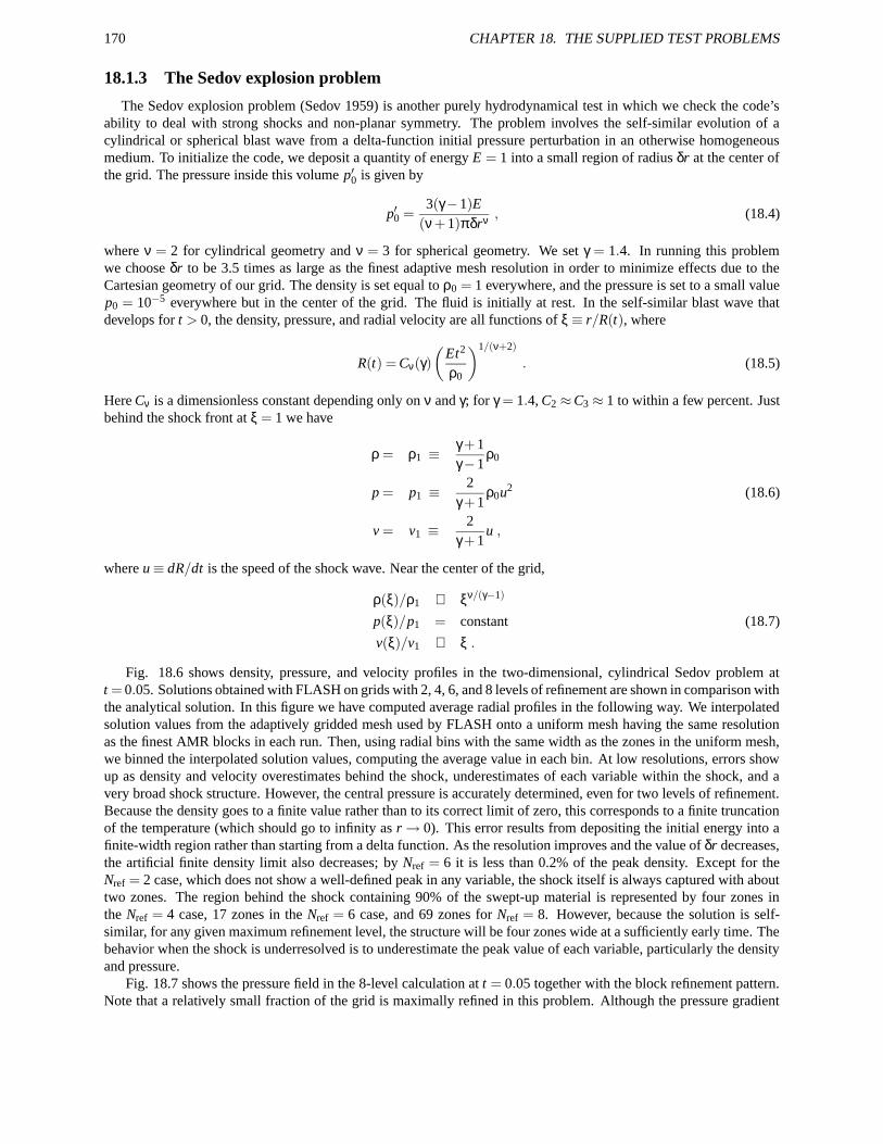
170 CHAPTER 18. THE SUPPLIED TEST PROBLEMS
18.1.3 The Sedov explosion problem
The Sedov explosion problem (Sedov 1959) is another purely hydrodynamical test in which we check the code’sability to deal with strong shocks and non-planar symmetry. The problem involves the self-similar evolution of acylindrical or spherical blast wave from a delta-function initial pressure perturbation in an otherwise homogeneousmedium. To initialize the code, we deposit a quantity of energy E = 1 into a small region of radius δr at the center ofthe grid. The pressure inside this volume p′0 is given by
p′0 =3(γ−1)E
(ν+1)πδrν , (18.4)
where ν = 2 for cylindrical geometry and ν = 3 for spherical geometry. We set γ = 1.4. In running this problemwe choose δr to be 3.5 times as large as the finest adaptive mesh resolution in order to minimize effects due to theCartesian geometry of our grid. The density is set equal to ρ0 = 1 everywhere, and the pressure is set to a small valuep0 = 10−5 everywhere but in the center of the grid. The fluid is initially at rest. In the self-similar blast wave thatdevelops for t > 0, the density, pressure, and radial velocity are all functions of ξ≡ r/R(t), where
R(t) = Cν(γ)(
Et2
ρ0
)1/(ν+2)
. (18.5)
Here Cν is a dimensionless constant depending only on ν and γ; for γ = 1.4, C2 ≈C3 ≈ 1 to within a few percent. Justbehind the shock front at ξ = 1 we have
ρ = ρ1 ≡γ+1γ−1
ρ0
p = p1 ≡2
γ+1ρ0u2 (18.6)
v = v1 ≡2
γ+1u ,
where u≡ dR/dt is the speed of the shock wave. Near the center of the grid,
ρ(ξ)/ρ1 ∝ ξν/(γ−1)
p(ξ)/p1 = constant (18.7)
v(ξ)/v1 ∝ ξ .
Fig. 18.6 shows density, pressure, and velocity profiles in the two-dimensional, cylindrical Sedov problem att = 0.05. Solutions obtained with FLASH on grids with 2, 4, 6, and 8 levels of refinement are shown in comparison withthe analytical solution. In this figure we have computed average radial profiles in the following way. We interpolatedsolution values from the adaptively gridded mesh used by FLASH onto a uniform mesh having the same resolutionas the finest AMR blocks in each run. Then, using radial bins with the same width as the zones in the uniform mesh,we binned the interpolated solution values, computing the average value in each bin. At low resolutions, errors showup as density and velocity overestimates behind the shock, underestimates of each variable within the shock, and avery broad shock structure. However, the central pressure is accurately determined, even for two levels of refinement.Because the density goes to a finite value rather than to its correct limit of zero, this corresponds to a finite truncationof the temperature (which should go to infinity as r→ 0). This error results from depositing the initial energy into afinite-width region rather than starting from a delta function. As the resolution improves and the value of δr decreases,the artificial finite density limit also decreases; by Nref = 6 it is less than 0.2% of the peak density. Except for theNref = 2 case, which does not show a well-defined peak in any variable, the shock itself is always captured with abouttwo zones. The region behind the shock containing 90% of the swept-up material is represented by four zones inthe Nref = 4 case, 17 zones in the Nref = 6 case, and 69 zones for Nref = 8. However, because the solution is self-similar, for any given maximum refinement level, the structure will be four zones wide at a sufficiently early time. Thebehavior when the shock is underresolved is to underestimate the peak value of each variable, particularly the densityand pressure.
Fig. 18.7 shows the pressure field in the 8-level calculation at t = 0.05 together with the block refinement pattern.Note that a relatively small fraction of the grid is maximally refined in this problem. Although the pressure gradient
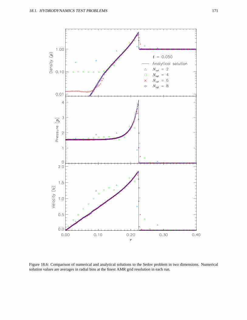
18.1. HYDRODYNAMICS TEST PROBLEMS 171
Figure 18.6: Comparison of numerical and analytical solutions to the Sedov problem in two dimensions. Numericalsolution values are averages in radial bins at the finest AMR grid resolution in each run.
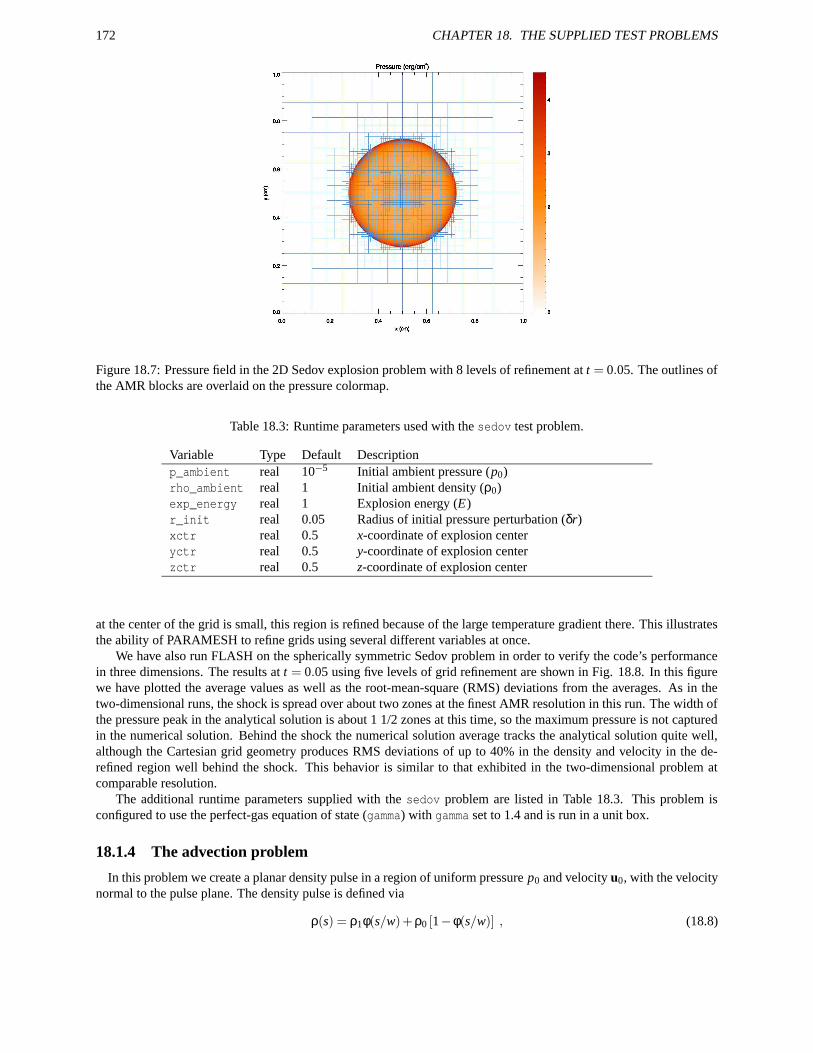
172 CHAPTER 18. THE SUPPLIED TEST PROBLEMS
Figure 18.7: Pressure field in the 2D Sedov explosion problem with 8 levels of refinement at t = 0.05. The outlines ofthe AMR blocks are overlaid on the pressure colormap.
Table 18.3: Runtime parameters used with the sedov test problem.
Variable Type Default Descriptionp_ambient real 10−5 Initial ambient pressure (p0)rho_ambient real 1 Initial ambient density (ρ0)exp_energy real 1 Explosion energy (E)r_init real 0.05 Radius of initial pressure perturbation (δr)xctr real 0.5 x-coordinate of explosion centeryctr real 0.5 y-coordinate of explosion centerzctr real 0.5 z-coordinate of explosion center
at the center of the grid is small, this region is refined because of the large temperature gradient there. This illustratesthe ability of PARAMESH to refine grids using several different variables at once.
We have also run FLASH on the spherically symmetric Sedov problem in order to verify the code’s performancein three dimensions. The results at t = 0.05 using five levels of grid refinement are shown in Fig. 18.8. In this figurewe have plotted the average values as well as the root-mean-square (RMS) deviations from the averages. As in thetwo-dimensional runs, the shock is spread over about two zones at the finest AMR resolution in this run. The width ofthe pressure peak in the analytical solution is about 1 1/2 zones at this time, so the maximum pressure is not capturedin the numerical solution. Behind the shock the numerical solution average tracks the analytical solution quite well,although the Cartesian grid geometry produces RMS deviations of up to 40% in the density and velocity in the de-refined region well behind the shock. This behavior is similar to that exhibited in the two-dimensional problem atcomparable resolution.
The additional runtime parameters supplied with the sedov problem are listed in Table 18.3. This problem isconfigured to use the perfect-gas equation of state (gamma) with gamma set to 1.4 and is run in a unit box.
18.1.4 The advection problem
In this problem we create a planar density pulse in a region of uniform pressure p0 and velocity u0, with the velocitynormal to the pulse plane. The density pulse is defined via
ρ(s) = ρ1φ(s/w)+ρ0 [1−φ(s/w)] , (18.8)
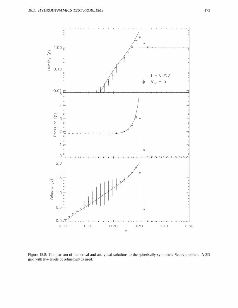
18.1. HYDRODYNAMICS TEST PROBLEMS 173
Figure 18.8: Comparison of numerical and analytical solutions to the spherically symmetric Sedov problem. A 3Dgrid with five levels of refinement is used.
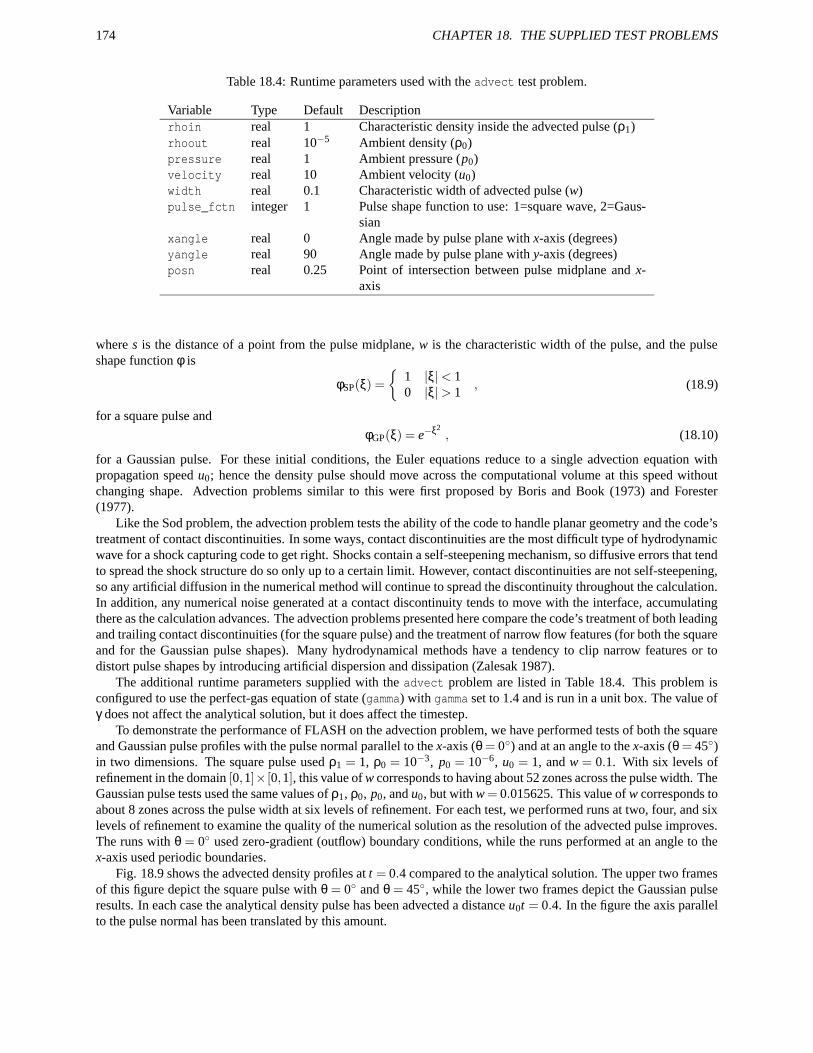
174 CHAPTER 18. THE SUPPLIED TEST PROBLEMS
Table 18.4: Runtime parameters used with the advect test problem.
Variable Type Default Descriptionrhoin real 1 Characteristic density inside the advected pulse (ρ1)rhoout real 10−5 Ambient density (ρ0)pressure real 1 Ambient pressure (p0)velocity real 10 Ambient velocity (u0)width real 0.1 Characteristic width of advected pulse (w)pulse_fctn integer 1 Pulse shape function to use: 1=square wave, 2=Gaus-
sianxangle real 0 Angle made by pulse plane with x-axis (degrees)yangle real 90 Angle made by pulse plane with y-axis (degrees)posn real 0.25 Point of intersection between pulse midplane and x-
axis
where s is the distance of a point from the pulse midplane, w is the characteristic width of the pulse, and the pulseshape function φ is
φSP(ξ) =
1 |ξ|< 10 |ξ|> 1
, (18.9)
for a square pulse and
φGP(ξ) = e−ξ2, (18.10)
for a Gaussian pulse. For these initial conditions, the Euler equations reduce to a single advection equation withpropagation speed u0; hence the density pulse should move across the computational volume at this speed withoutchanging shape. Advection problems similar to this were first proposed by Boris and Book (1973) and Forester(1977).
Like the Sod problem, the advection problem tests the ability of the code to handle planar geometry and the code’streatment of contact discontinuities. In some ways, contact discontinuities are the most difficult type of hydrodynamicwave for a shock capturing code to get right. Shocks contain a self-steepening mechanism, so diffusive errors that tendto spread the shock structure do so only up to a certain limit. However, contact discontinuities are not self-steepening,so any artificial diffusion in the numerical method will continue to spread the discontinuity throughout the calculation.In addition, any numerical noise generated at a contact discontinuity tends to move with the interface, accumulatingthere as the calculation advances. The advection problems presented here compare the code’s treatment of both leadingand trailing contact discontinuities (for the square pulse) and the treatment of narrow flow features (for both the squareand for the Gaussian pulse shapes). Many hydrodynamical methods have a tendency to clip narrow features or todistort pulse shapes by introducing artificial dispersion and dissipation (Zalesak 1987).
The additional runtime parameters supplied with the advect problem are listed in Table 18.4. This problem isconfigured to use the perfect-gas equation of state (gamma) with gamma set to 1.4 and is run in a unit box. The value ofγ does not affect the analytical solution, but it does affect the timestep.
To demonstrate the performance of FLASH on the advection problem, we have performed tests of both the squareand Gaussian pulse profiles with the pulse normal parallel to the x-axis (θ = 0) and at an angle to the x-axis (θ = 45)in two dimensions. The square pulse used ρ1 = 1, ρ0 = 10−3, p0 = 10−6, u0 = 1, and w = 0.1. With six levels ofrefinement in the domain [0,1]× [0,1], this value of w corresponds to having about 52 zones across the pulse width. TheGaussian pulse tests used the same values of ρ1, ρ0, p0, and u0, but with w = 0.015625. This value of w corresponds toabout 8 zones across the pulse width at six levels of refinement. For each test, we performed runs at two, four, and sixlevels of refinement to examine the quality of the numerical solution as the resolution of the advected pulse improves.The runs with θ = 0 used zero-gradient (outflow) boundary conditions, while the runs performed at an angle to thex-axis used periodic boundaries.
Fig. 18.9 shows the advected density profiles at t = 0.4 compared to the analytical solution. The upper two framesof this figure depict the square pulse with θ = 0 and θ = 45, while the lower two frames depict the Gaussian pulseresults. In each case the analytical density pulse has been advected a distance u0t = 0.4. In the figure the axis parallelto the pulse normal has been translated by this amount.
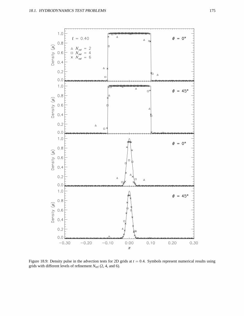
18.1. HYDRODYNAMICS TEST PROBLEMS 175
Figure 18.9: Density pulse in the advection tests for 2D grids at t = 0.4. Symbols represent numerical results usinggrids with different levels of refinement Nref (2, 4, and 6).
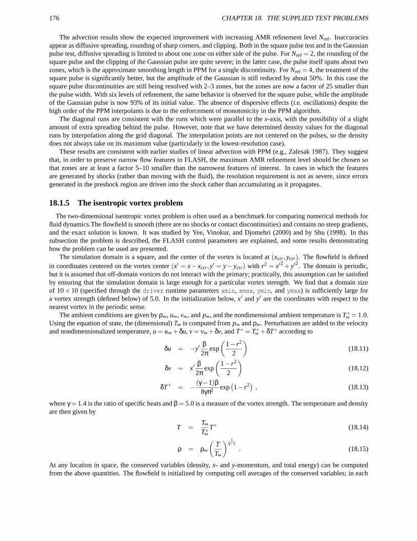
176 CHAPTER 18. THE SUPPLIED TEST PROBLEMS
The advection results show the expected improvement with increasing AMR refinement level Nref. Inaccuraciesappear as diffusive spreading, rounding of sharp corners, and clipping. Both in the square pulse test and in the Gaussianpulse test, diffusive spreading is limited to about one zone on either side of the pulse. For Nref = 2, the rounding of thesquare pulse and the clipping of the Gaussian pulse are quite severe; in the latter case, the pulse itself spans about twozones, which is the approximate smoothing length in PPM for a single discontinuity. For Nref = 4, the treatment of thesquare pulse is significantly better, but the amplitude of the Gaussian is still reduced by about 50%. In this case thesquare pulse discontinuities are still being resolved with 2–3 zones, but the zones are now a factor of 25 smaller thanthe pulse width. With six levels of refinement, the same behavior is observed for the square pulse, while the amplitudeof the Gaussian pulse is now 93% of its initial value. The absence of dispersive effects (i.e. oscillations) despite thehigh order of the PPM interpolants is due to the enforcement of monotonicity in the PPM algorithm.
The diagonal runs are consistent with the runs which were parallel to the x-axis, with the possibility of a slightamount of extra spreading behind the pulse. However, note that we have determined density values for the diagonalruns by interpolation along the grid diagonal. The interpolation points are not centered on the pulses, so the densitydoes not always take on its maximum value (particularly in the lowest-resolution case).
These results are consistent with earlier studies of linear advection with PPM (e.g., Zalesak 1987). They suggestthat, in order to preserve narrow flow features in FLASH, the maximum AMR refinement level should be chosen sothat zones are at least a factor 5–10 smaller than the narrowest features of interest. In cases in which the featuresare generated by shocks (rather than moving with the fluid), the resolution requirement is not as severe, since errorsgenerated in the preshock region are driven into the shock rather than accumulating as it propagates.
18.1.5 The isentropic vortex problem
The two-dimensional isentropic vortex problem is often used as a benchmark for comparing numerical methods forfluid dynamics.The flowfield is smooth (there are no shocks or contact discontinuities) and contains no steep gradients,and the exact solution is known. It was studied by Yee, Vinokur, and Djomehri (2000) and by Shu (1998). In thissubsection the problem is described, the FLASH control parameters are explained, and some results demonstratinghow the problem can be used are presented.
The simulation domain is a square, and the center of the vortex is located at (xctr,yctr). The flowfield is definedin coordinates centered on the vortex center (x′ = x− xctr,y′ = y− yctr) with r2 = x′2 + y′2. The domain is periodic,but it is assumed that off-domain vortices do not interact with the primary; practically, this assumption can be satisfiedby ensuring that the simulation domain is large enough for a particular vortex strength. We find that a domain sizeof 10× 10 (specified through the driver runtime parameters xmin, xmax, ymin, and ymax) is sufficiently large fora vortex strength (defined below) of 5.0. In the initialization below, x′ and y′ are the coordinates with respect to thenearest vortex in the periodic sense.
The ambient conditions are given by ρ∞, u∞, v∞, and p∞, and the nondimensional ambient temperature is T ∗∞ = 1.0.Using the equation of state, the (dimensional) T∞ is computed from p∞ and ρ∞. Perturbations are added to the velocityand nondimensionalized temperature, u = u∞ +δu, v = v∞ +δv, and T ∗ = T ∗∞ +δT ∗ according to
δu = −y′β2π
exp
(
1− r2
2
)
(18.11)
δv = x′β
2πexp
(
1− r2
2
)
(18.12)
δT ∗ = − (γ−1)β8γπ2 exp
(
1− r2) , (18.13)
where γ = 1.4 is the ratio of specific heats and β = 5.0 is a measure of the vortex strength. The temperature and densityare then given by
T =T∞
T ∗∞T ∗ (18.14)
ρ = ρ∞
(
TT∞
) 1γ−1
. (18.15)
At any location in space, the conserved variables (density, x- and y-momentum, and total energy) can be computedfrom the above quantities. The flowfield is initialized by computing cell averages of the conserved variables; in each
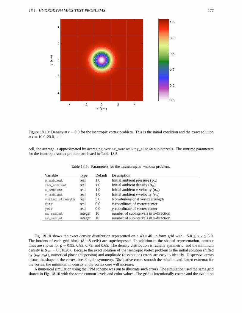
18.1. HYDRODYNAMICS TEST PROBLEMS 177
Figure 18.10: Density at t = 0.0 for the isentropic vortex problem. This is the initial condition and the exact solutionat t = 10.0,20.0, . . ..
cell, the average is approximated by averaging over nx_subint×ny_subint subintervals. The runtime parametersfor the isentropic vortex problem are listed in Table 18.5.
Table 18.5: Parameters for the isentropic_vortex problem.
Variable Type Default Descriptionp_ambient real 1.0 Initial ambient pressure (p∞)rho_ambient real 1.0 Initial ambient density (ρ∞)u_ambient real 1.0 Initial ambient x-velocity (u∞)v_ambient real 1.0 Initial ambient y-velocity (v∞)vortex_strength real 5.0 Non-dimensional vortex strengthxctr real 0.0 x-coordinate of vortex centeryctr real 0.0 y-coordinate of vortex centernx_subint integer 10 number of subintervals in x-directionny_subint integer 10 number of subintervals in y-direction
Fig. 18.10 shows the exact density distribution represented on a 40× 40 uniform grid with −5.0 ≤ x,y ≤ 5.0.The borders of each grid block (8× 8 cells) are superimposed. In addition to the shaded representation, contourlines are shown for ρ = 0.95, 0.85, 0.75, and 0.65. The density distribution is radially symmetric, and the minimumdensity is ρmin = 0.510287. Because the exact solution of the isentropic vortex problem is the initial solution shiftedby (u∞t,v∞t), numerical phase (dispersion) and amplitude (dissipation) errors are easy to identify. Dispersive errorsdistort the shape of the vortex, breaking its symmetry. Dissipative errors smooth the solution and flatten extrema; forthe vortex, the minimum in density at the vortex core will increase.
A numerical simulation using the PPM scheme was run to illustrate such errors. The simulation used the same gridshown in Fig. 18.10 with the same contour levels and color values. The grid is intentionally coarse and the evolution
178 CHAPTER 18. THE SUPPLIED TEST PROBLEMS
Figure 18.11: Density at t = 50.0 for the isentropic vortex problem.
time long to make numerical errors visible. The vortex is represented by approximately 8 grid points in each coordinatedirection and is advected diagonally with respect to the grid. At solution times of t = 10,20, . . ., etc., the vortex shouldbe back at its initial location.
Fig. 18.11 shows the solution at t = 50.0; only slight differences are observed. The density distribution is almostradially symmetric, although the minimum density has risen to 0.0537360. Accumulating dispersion error is clearlyvisible at t = 100.0 (Fig. 18.12), and the minimum density is now 0.601786.
Fig. 18.13 shows the density near y = 0.0 at three simulation times. The black line shows the initial condition.The red line corresponds to t = 50.0 and the blue line to t = 100.0. For the later two times, the density is not radiallysymmetric. The lines plotted are just representative profiles for those times, which give an idea of the magnitude andcharacter of the errors.
18.1.6 The problem of a wind tunnel with a step
The problem of a wind tunnel containing a step was first described by Emery (1968), who used it to compare severalhydrodynamical methods. Woodward and Colella (1984) later used it to compare several more advanced methods,including PPM. Although it has no analytical solution, this problem is useful because it exercises a code’s ability tohandle unsteady shock interactions in multiple dimensions. It also provides an example of the use of FLASH to solveproblems with irregular boundaries.
The problem uses a two-dimensional rectangular domain three units wide and one unit high. Between x = 0.6 andx = 3 along the x-axis is a step 0.2 units high. The step is treated as a reflecting boundary, as are the lower and upperboundaries in the y-direction. For the right-hand x-boundary, we use an outflow (zero gradient) boundary condition,while on the left-hand side we use an inflow boundary. In the inflow boundary zones, we set the density to ρ0, thepressure to p0, and the velocity to u0, with the latter directed parallel to the x-axis. The domain itself is also initializedwith these values. We use
ρ0 = 1.4, p0 = 1, u0 = 3 , γ = 1.4, (18.16)
which corresponds to a Mach 3 flow. Because the outflow is supersonic throughout the calculation, we do not expectreflections from the right-hand boundary.
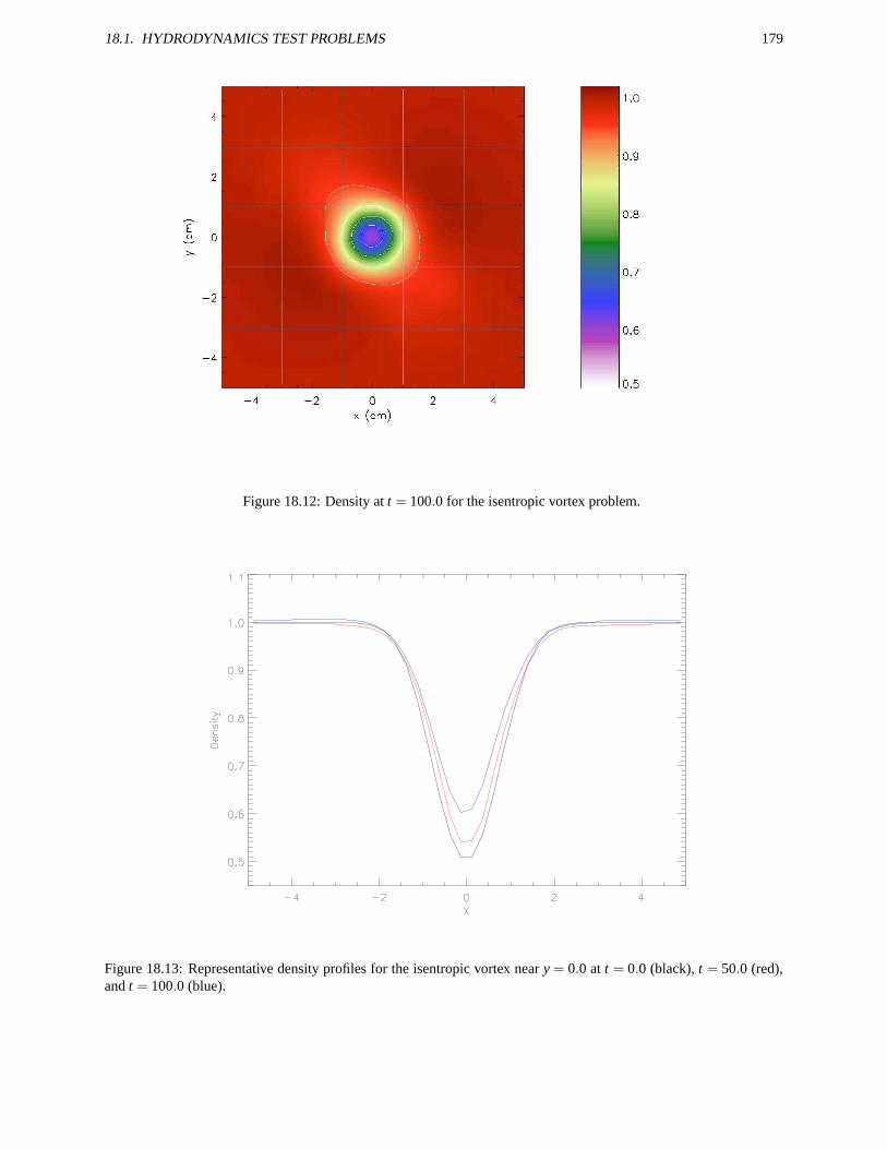
18.1. HYDRODYNAMICS TEST PROBLEMS 179
Figure 18.12: Density at t = 100.0 for the isentropic vortex problem.
Figure 18.13: Representative density profiles for the isentropic vortex near y = 0.0 at t = 0.0 (black), t = 50.0 (red),and t = 100.0 (blue).
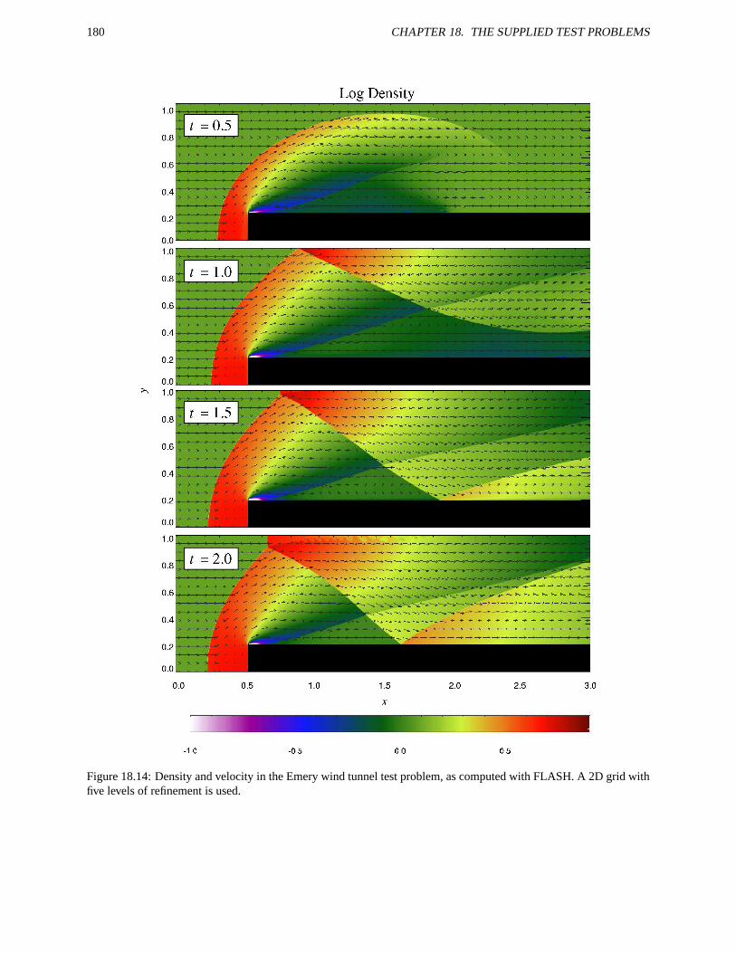
180 CHAPTER 18. THE SUPPLIED TEST PROBLEMS
Figure 18.14: Density and velocity in the Emery wind tunnel test problem, as computed with FLASH. A 2D grid withfive levels of refinement is used.
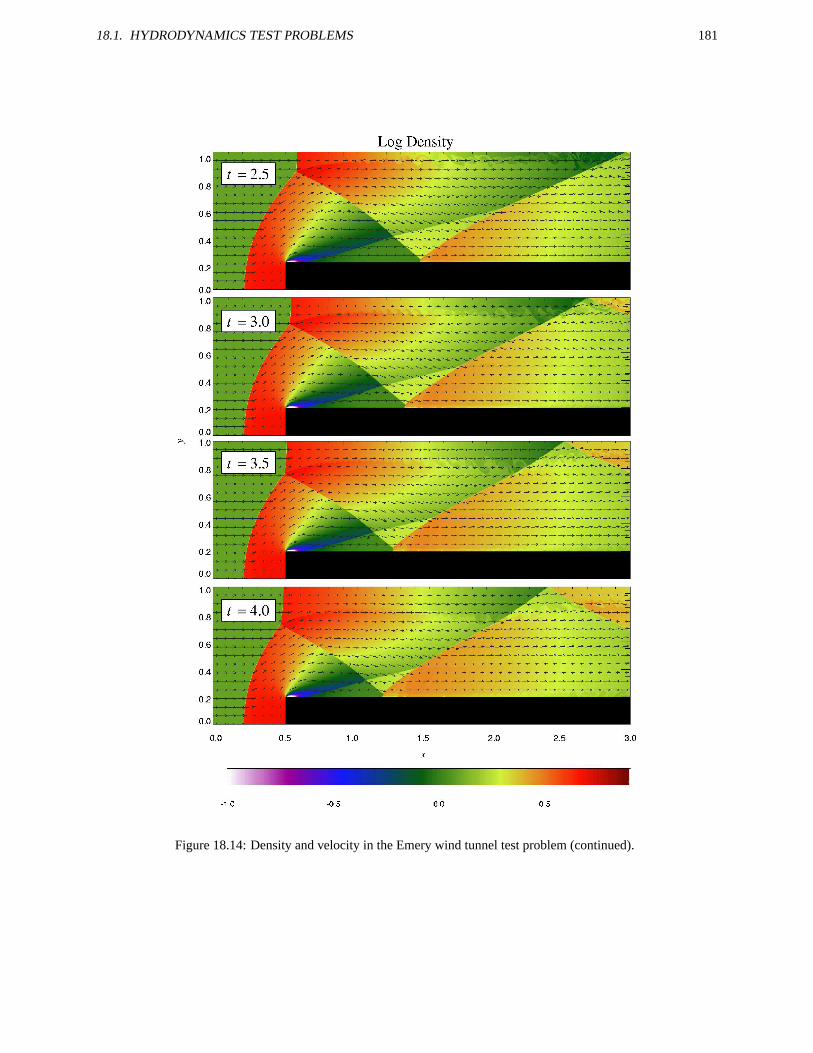
18.1. HYDRODYNAMICS TEST PROBLEMS 181
Figure 18.14: Density and velocity in the Emery wind tunnel test problem (continued).
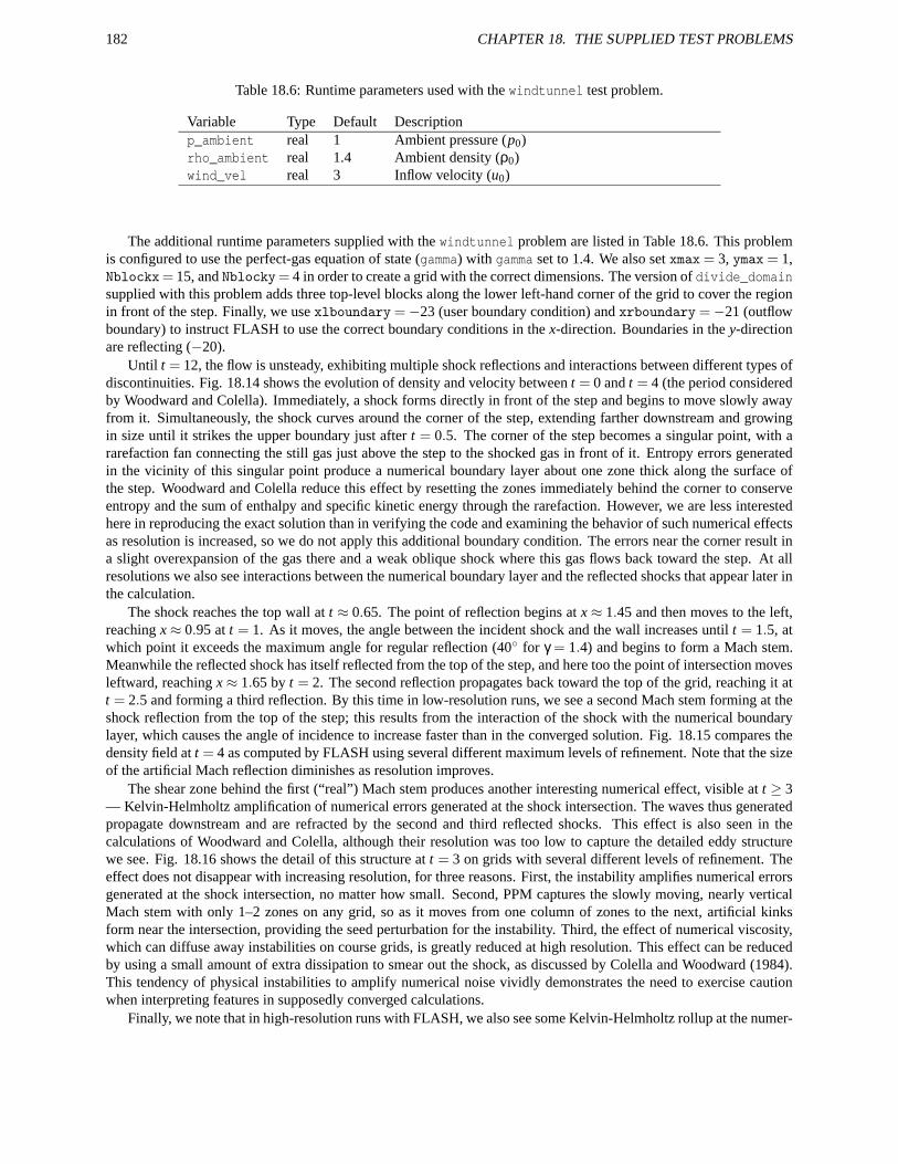
182 CHAPTER 18. THE SUPPLIED TEST PROBLEMS
Table 18.6: Runtime parameters used with the windtunnel test problem.
Variable Type Default Descriptionp_ambient real 1 Ambient pressure (p0)rho_ambient real 1.4 Ambient density (ρ0)wind_vel real 3 Inflow velocity (u0)
The additional runtime parameters supplied with the windtunnel problem are listed in Table 18.6. This problemis configured to use the perfect-gas equation of state (gamma) with gamma set to 1.4. We also set xmax = 3, ymax = 1,Nblockx= 15, and Nblocky= 4 in order to create a grid with the correct dimensions. The version of divide_domainsupplied with this problem adds three top-level blocks along the lower left-hand corner of the grid to cover the regionin front of the step. Finally, we use xlboundary =−23 (user boundary condition) and xrboundary =−21 (outflowboundary) to instruct FLASH to use the correct boundary conditions in the x-direction. Boundaries in the y-directionare reflecting (−20).
Until t = 12, the flow is unsteady, exhibiting multiple shock reflections and interactions between different types ofdiscontinuities. Fig. 18.14 shows the evolution of density and velocity between t = 0 and t = 4 (the period consideredby Woodward and Colella). Immediately, a shock forms directly in front of the step and begins to move slowly awayfrom it. Simultaneously, the shock curves around the corner of the step, extending farther downstream and growingin size until it strikes the upper boundary just after t = 0.5. The corner of the step becomes a singular point, with ararefaction fan connecting the still gas just above the step to the shocked gas in front of it. Entropy errors generatedin the vicinity of this singular point produce a numerical boundary layer about one zone thick along the surface ofthe step. Woodward and Colella reduce this effect by resetting the zones immediately behind the corner to conserveentropy and the sum of enthalpy and specific kinetic energy through the rarefaction. However, we are less interestedhere in reproducing the exact solution than in verifying the code and examining the behavior of such numerical effectsas resolution is increased, so we do not apply this additional boundary condition. The errors near the corner result ina slight overexpansion of the gas there and a weak oblique shock where this gas flows back toward the step. At allresolutions we also see interactions between the numerical boundary layer and the reflected shocks that appear later inthe calculation.
The shock reaches the top wall at t ≈ 0.65. The point of reflection begins at x ≈ 1.45 and then moves to the left,reaching x ≈ 0.95 at t = 1. As it moves, the angle between the incident shock and the wall increases until t = 1.5, atwhich point it exceeds the maximum angle for regular reflection (40 for γ = 1.4) and begins to form a Mach stem.Meanwhile the reflected shock has itself reflected from the top of the step, and here too the point of intersection movesleftward, reaching x ≈ 1.65 by t = 2. The second reflection propagates back toward the top of the grid, reaching it att = 2.5 and forming a third reflection. By this time in low-resolution runs, we see a second Mach stem forming at theshock reflection from the top of the step; this results from the interaction of the shock with the numerical boundarylayer, which causes the angle of incidence to increase faster than in the converged solution. Fig. 18.15 compares thedensity field at t = 4 as computed by FLASH using several different maximum levels of refinement. Note that the sizeof the artificial Mach reflection diminishes as resolution improves.
The shear zone behind the first (“real”) Mach stem produces another interesting numerical effect, visible at t ≥ 3— Kelvin-Helmholtz amplification of numerical errors generated at the shock intersection. The waves thus generatedpropagate downstream and are refracted by the second and third reflected shocks. This effect is also seen in thecalculations of Woodward and Colella, although their resolution was too low to capture the detailed eddy structurewe see. Fig. 18.16 shows the detail of this structure at t = 3 on grids with several different levels of refinement. Theeffect does not disappear with increasing resolution, for three reasons. First, the instability amplifies numerical errorsgenerated at the shock intersection, no matter how small. Second, PPM captures the slowly moving, nearly verticalMach stem with only 1–2 zones on any grid, so as it moves from one column of zones to the next, artificial kinksform near the intersection, providing the seed perturbation for the instability. Third, the effect of numerical viscosity,which can diffuse away instabilities on course grids, is greatly reduced at high resolution. This effect can be reducedby using a small amount of extra dissipation to smear out the shock, as discussed by Colella and Woodward (1984).This tendency of physical instabilities to amplify numerical noise vividly demonstrates the need to exercise cautionwhen interpreting features in supposedly converged calculations.
Finally, we note that in high-resolution runs with FLASH, we also see some Kelvin-Helmholtz rollup at the numer-
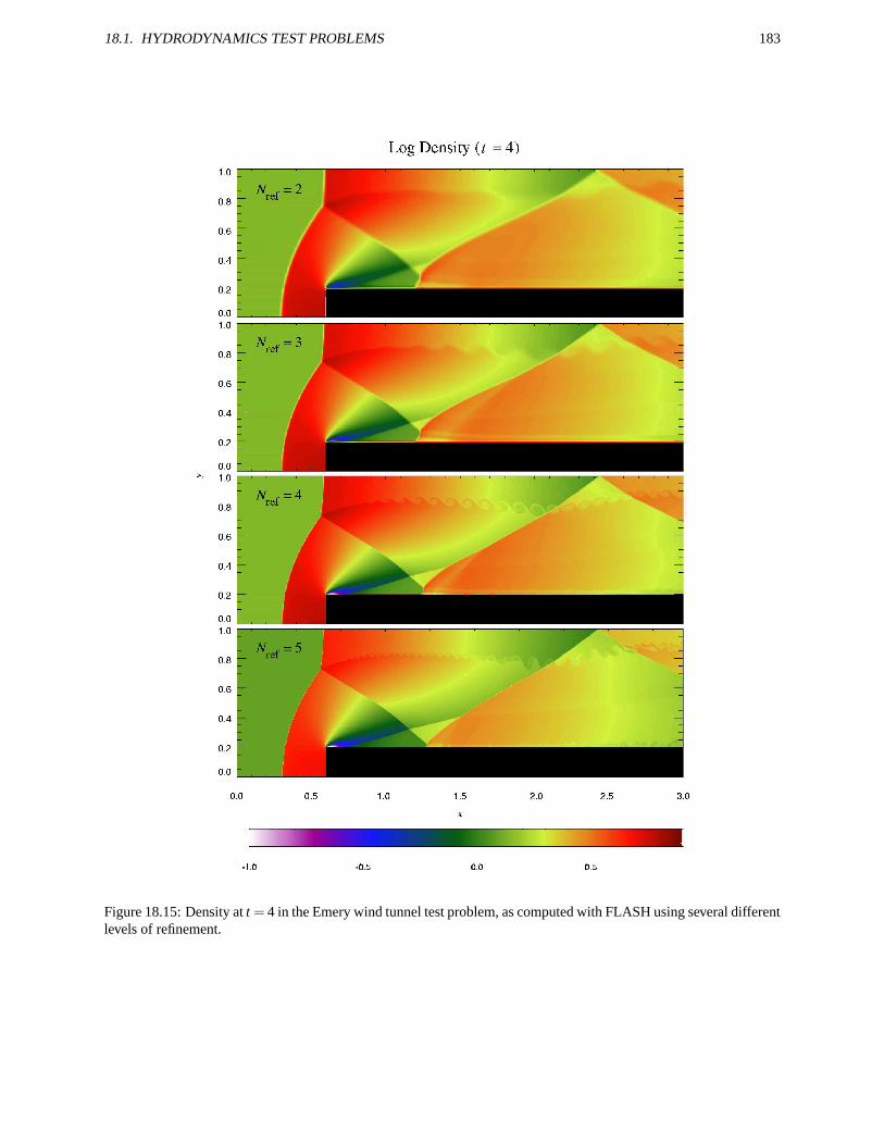
18.1. HYDRODYNAMICS TEST PROBLEMS 183
Figure 18.15: Density at t = 4 in the Emery wind tunnel test problem, as computed with FLASH using several differentlevels of refinement.
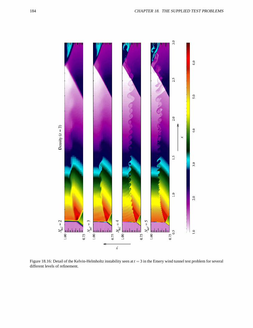
184 CHAPTER 18. THE SUPPLIED TEST PROBLEMS
Figure 18.16: Detail of the Kelvin-Helmholtz instability seen at t = 3 in the Emery wind tunnel test problem for severaldifferent levels of refinement.
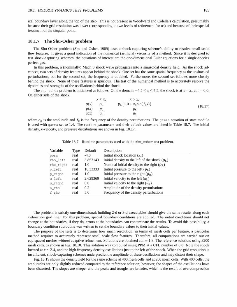
18.1. HYDRODYNAMICS TEST PROBLEMS 185
ical boundary layer along the top of the step. This is not present in Woodward and Colella’s calculation, presumablybecause their grid resolution was lower (corresponding to two levels of refinement for us) and because of their specialtreatment of the singular point.
18.1.7 The Shu-Osher problem
The Shu-Osher problem (Shu and Osher, 1989) tests a shock-capturing scheme’s ability to resolve small-scaleflow features. It gives a good indication of the numerical (artificial) viscosity of a method. Since it is designed totest shock-capturing schemes, the equations of interest are the one-dimensional Euler equations for a single-speciesperfect gas.
In this problem, a (nominally) Mach 3 shock wave propagates into a sinusoidal density field. As the shock ad-vances, two sets of density features appear behind the shock. One set has the same spatial frequency as the unshockedperturbations, but for the second set, the frequency is doubled. Furthermore, the second set follows more closelybehind the shock. None of these features is spurious. The test of the numerical method is to accurately resolve thedynamics and strengths of the oscillations behind the shock.
The shu_osher problem is initialized as follows. On the domain −4.5≤ x≤ 4.5, the shock is at x = xs at t = 0.0.On either side of the shock,
x≤ xs x > xsρ(x) ρL ρR
(
1.0+aρ sin( fρx))
p(x) pL pRu(x) uL uR
(18.17)
where aρ is the amplitude and fρ is the frequency of the density perturbations. The gamma equation of state moduleis used with gamma set to 1.4. The runtime parameters and their default values are listed in Table 18.7. The initialdensity, x-velocity, and pressure distributions are shown in Fig. 18.17.
Table 18.7: Runtime parameters used with the shu_osher test problem.
Variable Type Default Descriptionposn real -4.0 Initial shock location (xs)rho_left real 3.857143 Initial density to the left of the shock (ρL)rho_right real 1.0 Nominal initial density to the right (ρR)p_left real 10.33333 Initial pressure to the left (pL)p_right real 1.0 Initial pressure to the right (pR)u_left real 2.629369 Initial velocity to the left (uL)u_right real 0.0 Initial velocity to the right (uR)a_rho real 0.2 Amplitude of the density perturbationsf_rho real 5.0 Frequency of the density perturbations
The problem is strictly one-dimensional; building 2-d or 3-d executables should give the same results along eachx-direction grid line. For this problem, special boundary conditions are applied. The initial conditions should notchange at the boundaries; if they do, errors at the boundaries can contaminate the results. To avoid this possibility, aboundary condition subroutine was written to set the boundary values to their initial values.
The purpose of the tests is to determine how much resolution, in terms of mesh cells per feature, a particularmethod requires to accurately represent small scale flow features. Therefore, all computations are carried out onequispaced meshes without adaptive refinement. Solutions are obtained at t = 1.8. The reference solution, using 3200mesh cells, is shown in Fig. 18.18. This solution was computed using PPM at a CFL number of 0.8. Note the shocklocated at x' 2.4, and the high frequency density oscillations just to the left of the shock. When the grid resolution isinsufficient, shock-capturing schemes underpredict the amplitude of these oscillations and may distort their shape.
Fig. 18.19 shows the density field for the same scheme at 400 mesh cells and at 200 mesh cells. With 400 cells, theamplitudes are only slightly reduced compared to the reference solution; however, the shapes of the oscillations havebeen distorted. The slopes are steeper and the peaks and troughs are broader, which is the result of overcompression
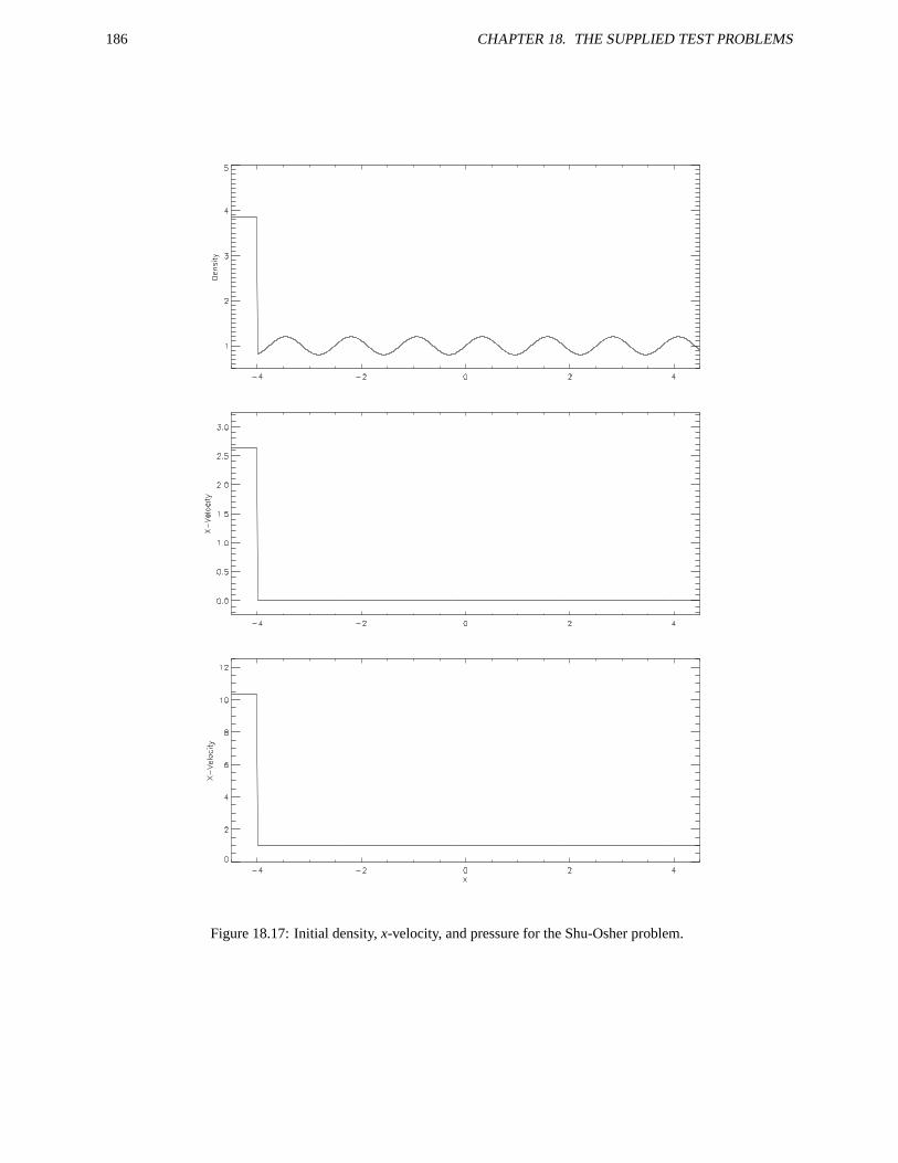
186 CHAPTER 18. THE SUPPLIED TEST PROBLEMS
Figure 18.17: Initial density, x-velocity, and pressure for the Shu-Osher problem.
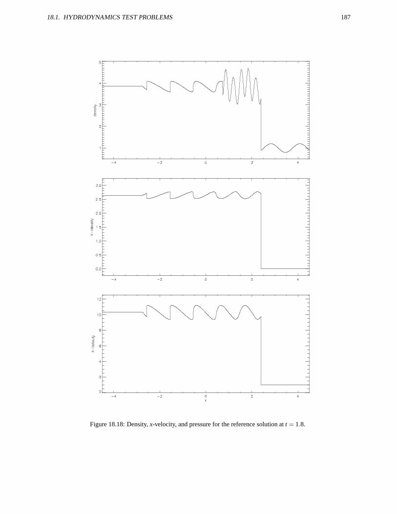
18.1. HYDRODYNAMICS TEST PROBLEMS 187
Figure 18.18: Density, x-velocity, and pressure for the reference solution at t = 1.8.
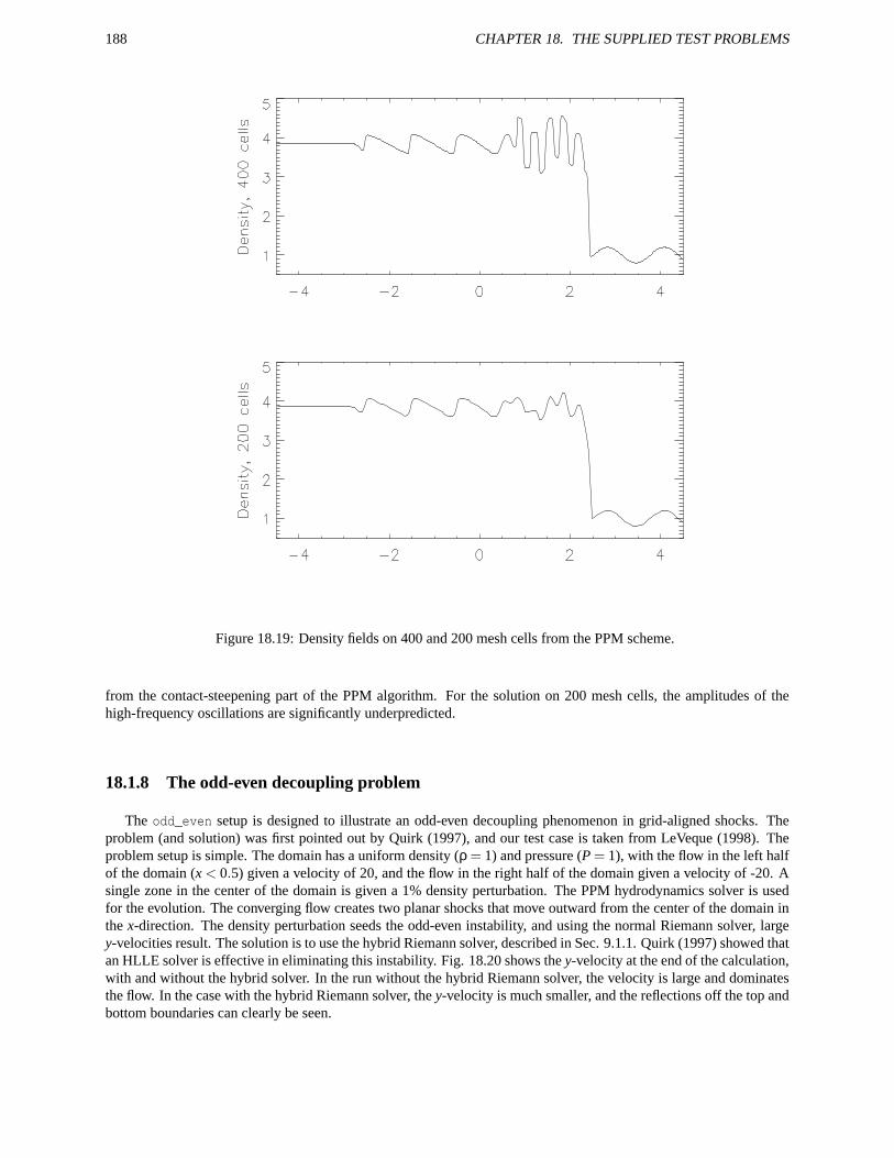
188 CHAPTER 18. THE SUPPLIED TEST PROBLEMS
Figure 18.19: Density fields on 400 and 200 mesh cells from the PPM scheme.
from the contact-steepening part of the PPM algorithm. For the solution on 200 mesh cells, the amplitudes of thehigh-frequency oscillations are significantly underpredicted.
18.1.8 The odd-even decoupling problem
The odd_even setup is designed to illustrate an odd-even decoupling phenomenon in grid-aligned shocks. Theproblem (and solution) was first pointed out by Quirk (1997), and our test case is taken from LeVeque (1998). Theproblem setup is simple. The domain has a uniform density (ρ = 1) and pressure (P = 1), with the flow in the left halfof the domain (x < 0.5) given a velocity of 20, and the flow in the right half of the domain given a velocity of -20. Asingle zone in the center of the domain is given a 1% density perturbation. The PPM hydrodynamics solver is usedfor the evolution. The converging flow creates two planar shocks that move outward from the center of the domain inthe x-direction. The density perturbation seeds the odd-even instability, and using the normal Riemann solver, largey-velocities result. The solution is to use the hybrid Riemann solver, described in Sec. 9.1.1. Quirk (1997) showed thatan HLLE solver is effective in eliminating this instability. Fig. 18.20 shows the y-velocity at the end of the calculation,with and without the hybrid solver. In the run without the hybrid Riemann solver, the velocity is large and dominatesthe flow. In the case with the hybrid Riemann solver, the y-velocity is much smaller, and the reflections off the top andbottom boundaries can clearly be seen.
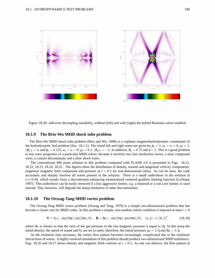
18.1. HYDRODYNAMICS TEST PROBLEMS 189
Figure 18.20: odd-even decoupling instability, without (left) and with (right) the hybrid Riemann solver enabled.
18.1.9 The Brio-Wu MHD shock tube problem
The Brio-Wu MHD shock tube problem (Brio and Wu, 1988) is a coplanar magnetohydrodynamic counterpart ofthe hydrodynamic Sod problem (Sec. 18.1.1). The initial left and right states are given by ρl = 1, ul = vl = 0, pl = 1,(By)l = 1; and ρr = 0.125, ur = vr = 0, pr = 0.1, (By)r =−1. In addition, Bx = 0.75 and γ = 2. This is a good problemto test wave properties of a particular MHD solver, because it involves two fast rarefaction waves, a slow compoundwave, a contact discontinuity and a slow shock wave.
The conventional 800 point solution to this problem computed with FLASH 2.0 is presented in Figs. 18.21,18.22, 18.23, 18.24, 18.25 . The figures show the distribution of density, normal and tangential velocity components,tangential magnetic field component and pressure at t = 0.1 (in non-dimensional units). As can be seen, the codeaccurately and sharply resolves all waves present in the solution. There is a small undershoot in the solution atx ≈ 0.44, which results from a discontinuity-enhancing monotonized centered gradient limiting function (LeVeque1997). This undershoot can be easily removed if a less aggressive limiter, e.g. a minmod or a van Leer limiter, is usedinstead. This, however, will degrade the sharp resolution of other discontinuities.
18.1.10 The Orszag-Tang MHD vortex problem
The Orszag-Tang MHD vortex problem (Orszag and Tang, 1979) is a simple two-dimensional problem that hasbecome a classic test for MHD codes. In this problem a simple, non-random initial condition is imposed at time t = 0
V = V0 (−sin(2πy),sin(2πx),0) , B = B0 (−sin(2πy),sin(4πx),0) , (x,y) =∈ [0,1]2, (18.18)
where B0 is chosen so that the ratio of the gas pressure to the rms magnetic pressure is equal to 2γ. In this setup theinitial density, the speed of sound and V0 are set to unity; therefore, the initial pressure p0 = 1/γ and B0 = 1/γ.
As the evolution time increases, the vortex flow pattern becomes increasingly complicated due to the nonlinearinteractions of waves. A highly resolved simulation of this problem should produce two-dimensional MHD turbulence.Figs. 18.26 and 18.27 shows density and magnetic field contours at t = 0.5. As one can observe, the flow pattern at
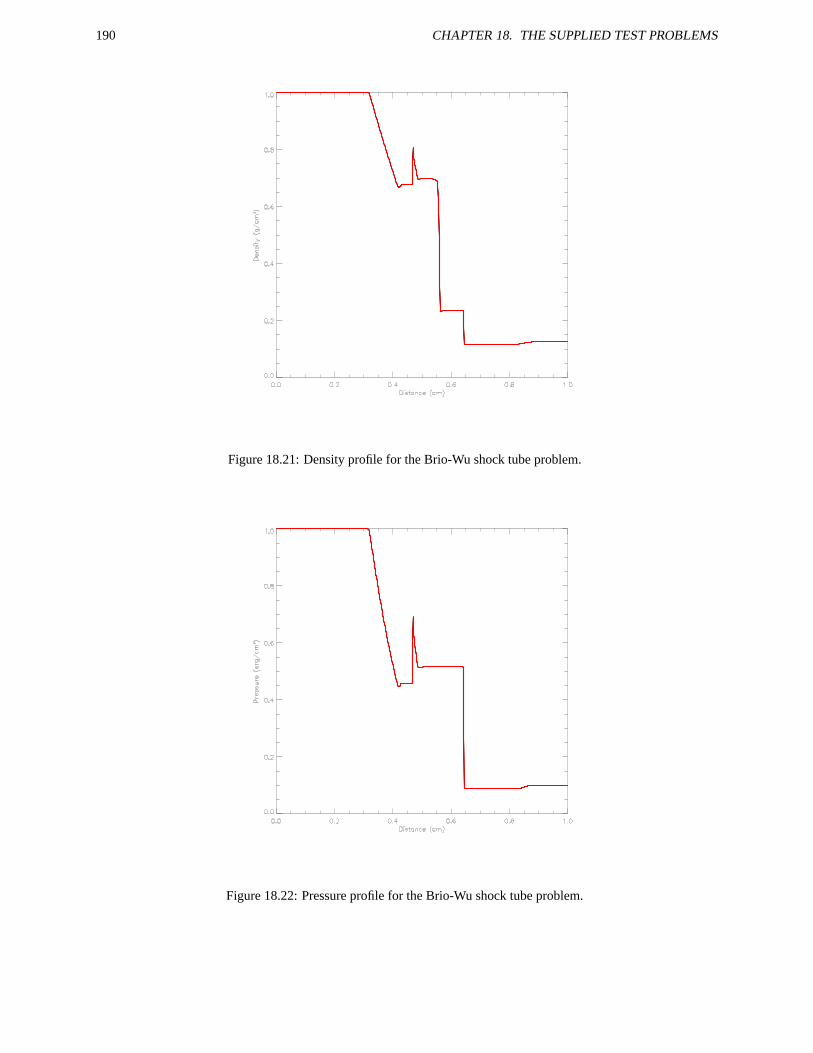
190 CHAPTER 18. THE SUPPLIED TEST PROBLEMS
Figure 18.21: Density profile for the Brio-Wu shock tube problem.
Figure 18.22: Pressure profile for the Brio-Wu shock tube problem.
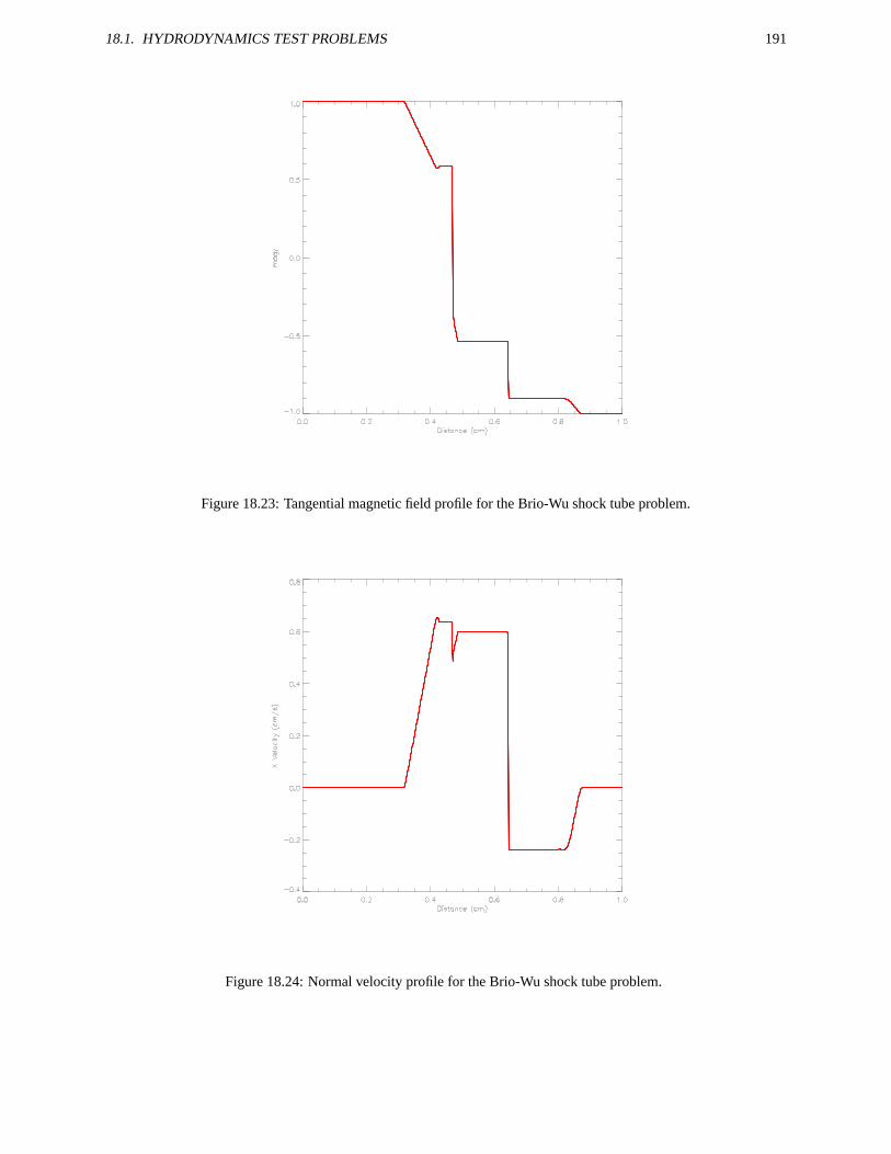
18.1. HYDRODYNAMICS TEST PROBLEMS 191
Figure 18.23: Tangential magnetic field profile for the Brio-Wu shock tube problem.
Figure 18.24: Normal velocity profile for the Brio-Wu shock tube problem.
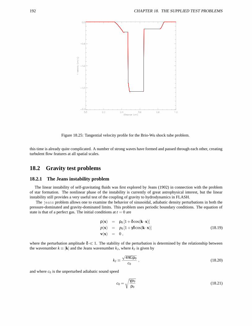
192 CHAPTER 18. THE SUPPLIED TEST PROBLEMS
Figure 18.25: Tangential velocity profile for the Brio-Wu shock tube problem.
this time is already quite complicated. A number of strong waves have formed and passed through each other, creatingturbulent flow features at all spatial scales.
18.2 Gravity test problems
18.2.1 The Jeans instability problem
The linear instability of self-gravitating fluids was first explored by Jeans (1902) in connection with the problemof star formation. The nonlinear phase of the instability is currently of great astrophysical interest, but the linearinstability still provides a very useful test of the coupling of gravity to hydrodynamics in FLASH.
The jeans problem allows one to examine the behavior of sinusoidal, adiabatic density perturbations in both thepressure-dominated and gravity-dominated limits. This problem uses periodic boundary conditions. The equation ofstate is that of a perfect gas. The initial conditions at t = 0 are
ρ(x) = ρ0 [1+δcos(k ·x)]
p(x) = p0 [1+ γδcos(k ·x)] (18.19)
v(x) = 0 ,
where the perturbation amplitude δ 1. The stability of the perturbation is determined by the relationship betweenthe wavenumber k ≡ |k| and the Jeans wavenumber kJ , where kJ is given by
kJ ≡√
4πGρ0
c0, (18.20)
and where c0 is the unperturbed adiabatic sound speed
c0 =
√
γp0
ρ0(18.21)
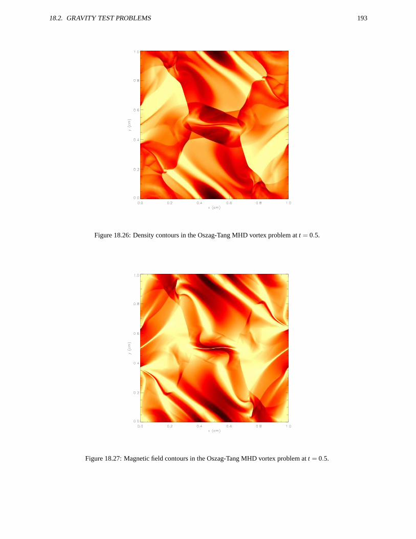
18.2. GRAVITY TEST PROBLEMS 193
Figure 18.26: Density contours in the Oszag-Tang MHD vortex problem at t = 0.5.
Figure 18.27: Magnetic field contours in the Oszag-Tang MHD vortex problem at t = 0.5.
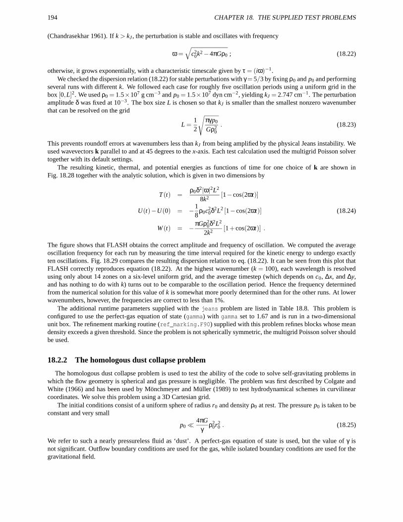
194 CHAPTER 18. THE SUPPLIED TEST PROBLEMS
(Chandrasekhar 1961). If k > kJ , the perturbation is stable and oscillates with frequency
ω =√
c20k2−4πGρ0 ; (18.22)
otherwise, it grows exponentially, with a characteristic timescale given by τ = (iω)−1.We checked the dispersion relation (18.22) for stable perturbations with γ = 5/3 by fixing ρ0 and p0 and performing
several runs with different k. We followed each case for roughly five oscillation periods using a uniform grid in thebox [0,L]2. We used ρ0 = 1.5×10⁷ g cm−3 and p0 = 1.5×10⁷ dyn cm−2, yielding kJ = 2.747 cm−1. The perturbationamplitude δ was fixed at 10−3. The box size L is chosen so that kJ is smaller than the smallest nonzero wavenumberthat can be resolved on the grid
L =12
√
πγp0
Gρ20
. (18.23)
This prevents roundoff errors at wavenumbers less than kJ from being amplified by the physical Jeans instability. Weused wavevectors k parallel to and at 45 degrees to the x-axis. Each test calculation used the multigrid Poisson solvertogether with its default settings.
The resulting kinetic, thermal, and potential energies as functions of time for one choice of k are shown inFig. 18.28 together with the analytic solution, which is given in two dimensions by
T (t) =ρ0δ2|ω|2L2
8k2 [1− cos(2ωt)]
U(t)−U(0) = −18
ρ0c20δ2L2 [1− cos(2ωt)] (18.24)
W (t) = −πGρ20δ2L2
2k2 [1+ cos(2ωt)] .
The figure shows that FLASH obtains the correct amplitude and frequency of oscillation. We computed the averageoscillation frequency for each run by measuring the time interval required for the kinetic energy to undergo exactlyten oscillations. Fig. 18.29 compares the resulting dispersion relation to eq. (18.22). It can be seen from this plot thatFLASH correctly reproduces equation (18.22). At the highest wavenumber (k = 100), each wavelength is resolvedusing only about 14 zones on a six-level uniform grid, and the average timestep (which depends on c0, ∆x, and ∆y,and has nothing to do with k) turns out to be comparable to the oscillation period. Hence the frequency determinedfrom the numerical solution for this value of k is somewhat more poorly determined than for the other runs. At lowerwavenumbers, however, the frequencies are correct to less than 1%.
The additional runtime parameters supplied with the jeans problem are listed in Table 18.8. This problem isconfigured to use the perfect-gas equation of state (gamma) with gamma set to 1.67 and is run in a two-dimensionalunit box. The refinement marking routine (ref_marking.F90) supplied with this problem refines blocks whose meandensity exceeds a given threshold. Since the problem is not spherically symmetric, the multigrid Poisson solver shouldbe used.
18.2.2 The homologous dust collapse problem
The homologous dust collapse problem is used to test the ability of the code to solve self-gravitating problems inwhich the flow geometry is spherical and gas pressure is negligible. The problem was first described by Colgate andWhite (1966) and has been used by Mönchmeyer and Müller (1989) to test hydrodynamical schemes in curvilinearcoordinates. We solve this problem using a 3D Cartesian grid.
The initial conditions consist of a uniform sphere of radius r0 and density ρ0 at rest. The pressure p0 is taken to beconstant and very small
p04πG
γρ2
0r20 . (18.25)
We refer to such a nearly pressureless fluid as ‘dust’. A perfect-gas equation of state is used, but the value of γ isnot significant. Outflow boundary conditions are used for the gas, while isolated boundary conditions are used for thegravitational field.
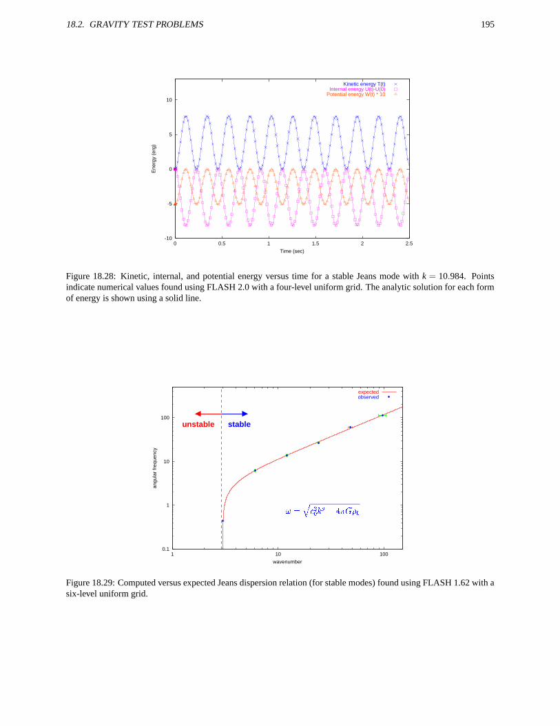
18.2. GRAVITY TEST PROBLEMS 195
-10
-5
0
5
10
0 0.5 1 1.5 2 2.5
Ene
rgy
(erg
)
Time (sec)
Kinetic energy T(t)Internal energy U(t)-U(0)
Potential energy W(t) * 10
Figure 18.28: Kinetic, internal, and potential energy versus time for a stable Jeans mode with k = 10.984. Pointsindicate numerical values found using FLASH 2.0 with a four-level uniform grid. The analytic solution for each formof energy is shown using a solid line.
0.1
1
10
100
1 10 100
angu
lar
freq
uenc
y
wavenumber
expectedobserved
unstable stable
Figure 18.29: Computed versus expected Jeans dispersion relation (for stable modes) found using FLASH 1.62 with asix-level uniform grid.
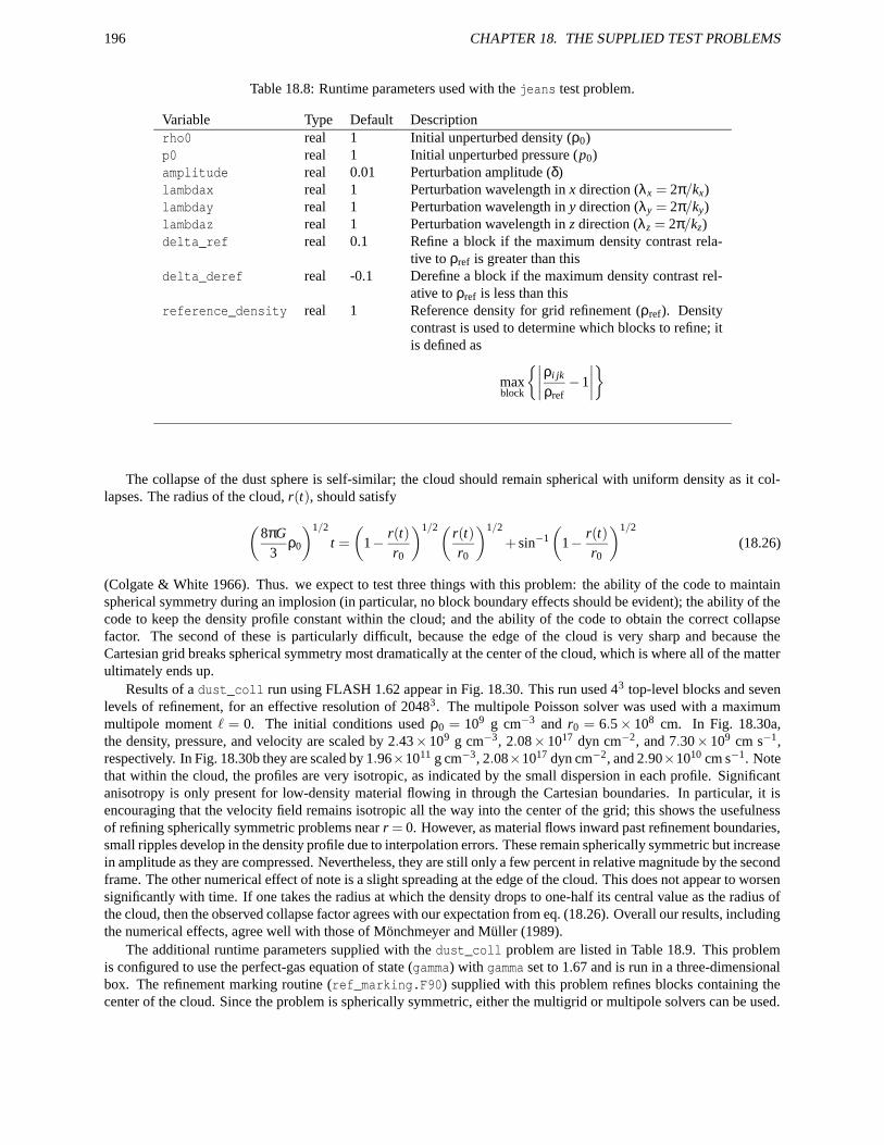
196 CHAPTER 18. THE SUPPLIED TEST PROBLEMS
Table 18.8: Runtime parameters used with the jeans test problem.
Variable Type Default Descriptionrho0 real 1 Initial unperturbed density (ρ0)p0 real 1 Initial unperturbed pressure (p0)amplitude real 0.01 Perturbation amplitude (δ)lambdax real 1 Perturbation wavelength in x direction (λx = 2π/kx)lambday real 1 Perturbation wavelength in y direction (λy = 2π/ky)lambdaz real 1 Perturbation wavelength in z direction (λz = 2π/kz)delta_ref real 0.1 Refine a block if the maximum density contrast rela-
tive to ρref is greater than thisdelta_deref real -0.1 Derefine a block if the maximum density contrast rel-
ative to ρref is less than thisreference_density real 1 Reference density for grid refinement (ρref). Density
contrast is used to determine which blocks to refine; itis defined as
maxblock
∣
∣
∣
∣
ρi jk
ρref−1
∣
∣
∣
∣
The collapse of the dust sphere is self-similar; the cloud should remain spherical with uniform density as it col-lapses. The radius of the cloud, r(t), should satisfy
(
8πG3
ρ0
)1/2
t =
(
1− r(t)r0
)1/2( r(t)r0
)1/2
+ sin−1(
1− r(t)r0
)1/2
(18.26)
(Colgate & White 1966). Thus. we expect to test three things with this problem: the ability of the code to maintainspherical symmetry during an implosion (in particular, no block boundary effects should be evident); the ability of thecode to keep the density profile constant within the cloud; and the ability of the code to obtain the correct collapsefactor. The second of these is particularly difficult, because the edge of the cloud is very sharp and because theCartesian grid breaks spherical symmetry most dramatically at the center of the cloud, which is where all of the matterultimately ends up.
Results of a dust_coll run using FLASH 1.62 appear in Fig. 18.30. This run used 43 top-level blocks and sevenlevels of refinement, for an effective resolution of 20483. The multipole Poisson solver was used with a maximummultipole moment ` = 0. The initial conditions used ρ0 = 109 g cm−3 and r0 = 6.5× 108 cm. In Fig. 18.30a,the density, pressure, and velocity are scaled by 2.43× 10⁹ g cm−3, 2.08× 10¹⁷ dyn cm−2, and 7.30× 109 cm s−1,respectively. In Fig. 18.30b they are scaled by 1.96×10¹¹ g cm−3, 2.08×10¹⁷ dyn cm−2, and 2.90×1010 cm s−1. Notethat within the cloud, the profiles are very isotropic, as indicated by the small dispersion in each profile. Significantanisotropy is only present for low-density material flowing in through the Cartesian boundaries. In particular, it isencouraging that the velocity field remains isotropic all the way into the center of the grid; this shows the usefulnessof refining spherically symmetric problems near r = 0. However, as material flows inward past refinement boundaries,small ripples develop in the density profile due to interpolation errors. These remain spherically symmetric but increasein amplitude as they are compressed. Nevertheless, they are still only a few percent in relative magnitude by the secondframe. The other numerical effect of note is a slight spreading at the edge of the cloud. This does not appear to worsensignificantly with time. If one takes the radius at which the density drops to one-half its central value as the radius ofthe cloud, then the observed collapse factor agrees with our expectation from eq. (18.26). Overall our results, includingthe numerical effects, agree well with those of Mönchmeyer and Müller (1989).
The additional runtime parameters supplied with the dust_coll problem are listed in Table 18.9. This problemis configured to use the perfect-gas equation of state (gamma) with gamma set to 1.67 and is run in a three-dimensionalbox. The refinement marking routine (ref_marking.F90) supplied with this problem refines blocks containing thecenter of the cloud. Since the problem is spherically symmetric, either the multigrid or multipole solvers can be used.
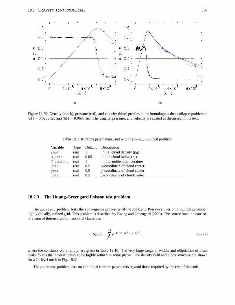
18.2. GRAVITY TEST PROBLEMS 197
(a) (b)
Figure 18.30: Density (black), pressure (red), and velocity (blue) profiles in the homologous dust collapse problem at(a) t = 0.0368 sec and (b) t = 0.0637 sec. The density, pressure, and velocity are scaled as discussed in the text.
Table 18.9: Runtime parameters used with the dust_coll test problem.
Variable Type Default Descriptionrho0 real 1 Initial cloud density (ρ0)R_init real 0.05 Initial cloud radius (r0)T_ambient real 1 Initial ambient temperaturexctr real 0.5 x-coordinate of cloud centeryctr real 0.5 y-coordinate of cloud centerzctr real 0.5 z-coordinate of cloud center
18.2.3 The Huang-Greengard Poisson test problem
The poistest problem tests the convergence properties of the multigrid Poisson solver on a multidimensional,highly (locally) refined grid. This problem is described by Huang and Greengard (2000). The source function consistsof a sum of thirteen two-dimensional Gaussians
ρ(x,y) =13
∑i=1
e−σi[(x−xi)2+(y−yi)
2] , (18.27)
where the constants σi, xi, and yi are given in Table 18.10. The very large range of widths and ellipticities of thesepeaks forces the mesh structure to be highly refined in some places. The density field and block structure are shownfor a 14-level mesh in Fig. 18.31.
The poistest problem uses no additional runtime parameters beyond those required by the rest of the code.
198 CHAPTER 18. THE SUPPLIED TEST PROBLEMS
Figure 18.31: Density field and block structure for a 14-level mesh applied to the Huang-Greengard test problem. Theeffective resolution of the mesh is 65,5362.
Table 18.10: Constants used in the poistest problem.
i 1 2 3 4 5 6 7xi 0 -1 -1 0.28125 0.5 0.3046875 0.3046875yi 0 0.09375 1 0.53125 0.53125 0.1875 0.125σi 0.01 4000 20000 80000 16 360000 400000
i 8 9 10 11 12 13xi 0.375 0.5625 -0.5 -0.125 0.296875 0.5234375yi 0.15625 -0.125 -0.703125 -0.703125 -0.609375 -0.78125σi 2000 18200 128 49000 37000 18900
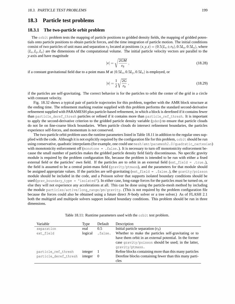
18.3. PARTICLE TEST PROBLEMS 199
18.3 Particle test problems
18.3.1 The two-particle orbit problem
The orbit problem tests the mapping of particle positions to gridded density fields, the mapping of gridded poten-tials onto particle positions to obtain particle forces, and the time integration of particle motion. The initial conditionsconsist of two particles of unit mass and separation r0 located at positions (x,y,z) = (0.5(Lx±r0),0.5Ly,0.5Lz), where(Lx,Ly,Lz) are the dimensions of the computational volume. The initial particle velocity vectors are parallel to they-axis and have magnitude
|v|=√
2GMr0
, (18.28)
if a constant gravitational field due to a point mass M at (0.5Lx,0.5Ly,0.5Lz) is employed, or
|v|= 12
√
2Gr0
, (18.29)
if the particles are self-gravitating. The correct behavior is for the particles to orbit the center of the grid in a circlewith constant velocity.
Fig. 18.32 shows a typical pair of particle trajectories for this problem, together with the AMR block structure atthe ending time. The refinement marking routine supplied with this problem performs the standard second-derivativerefinement supplied with PARAMESH plus particle-based refinement, in which a block is derefined if it contains fewerthan particle_deref_thresh particles or refined if it contains more than particle_ref_thresh. It is importantto apply the second-derivative criterion to the gridded particle density variable (pden) to ensure that particle cloudsdo not lie on fine-coarse block boundaries. When particle clouds do intersect refinement boundaries, the particlesexperience self-forces, and momentum is not conserved.
The two-particle orbit problem uses the runtime parameters listed in Table 18.11 in addition to the regular ones sup-plied with the code. Although it is not explicitly required by the configuration file for this problem, orbit should be runusing conservative, quadratic interpolants (for example, one could use mesh/amr/paramesh2.0/quadratic_cartesian)with monotonicity enforcement off (monotone = .false.). It is necessary to turn off monotonicity enforcement be-cause the small number of particles makes the gridded particle density field fairly discontinuous. No specific gravitymodule is required by the problem configuration file, because the problem is intended to be run with either a fixedexternal field or the particles’ own field. If the particles are to orbit in an external field (ext_field = .true.),the field is assumed to be a central point-mass field (gravity/ptmass), and the parameters for that module shouldbe assigned appropriate values. If the particles are self-gravitating (ext_field = .false.), the gravity/poissonmodule should be included in the code, and a Poisson solver that supports isolated boundary conditions should beused (grav_boundary_type = "isolated"). In either case, long-range forces for the particles must be turned on, orelse they will not experience any accelerations at all. This can be done using the particle-mesh method by includingthe module particles/active/long_range/pm/gravity. (This is not required by the problem configuration filebecause the forces could also be obtained using a future direct N-body solver or a tree solver.) As of FLASH 2.1both the multigrid and multipole solvers support isolated boundary conditions. This problem should be run in threedimensions.
Table 18.11: Runtime parameters used with the orbit test problem.
Variable Type Default Descriptionseparation real 0.5 Initial particle separation (r0)ext_field logical .false. Whether to make the particles self-gravitating or to
have them orbit in an external potential. In the formercase gravity/poisson should be used; in the latter,gravity/ptmass.
particle_ref_thresh integer 1 Refine blocks containing more than this many particlesparticle_deref_thresh integer 0 Derefine blocks containing fewer than this many parti-
cles
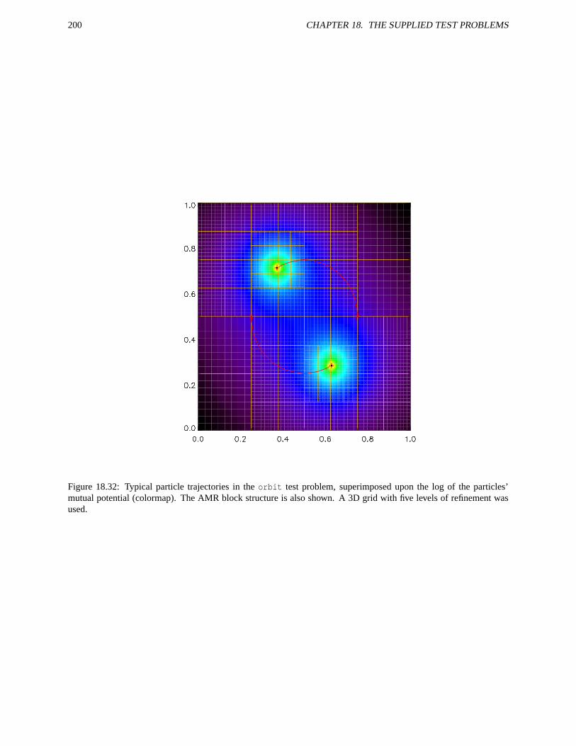
200 CHAPTER 18. THE SUPPLIED TEST PROBLEMS
Figure 18.32: Typical particle trajectories in the orbit test problem, superimposed upon the log of the particles’mutual potential (colormap). The AMR block structure is also shown. A 3D grid with five levels of refinement wasused.
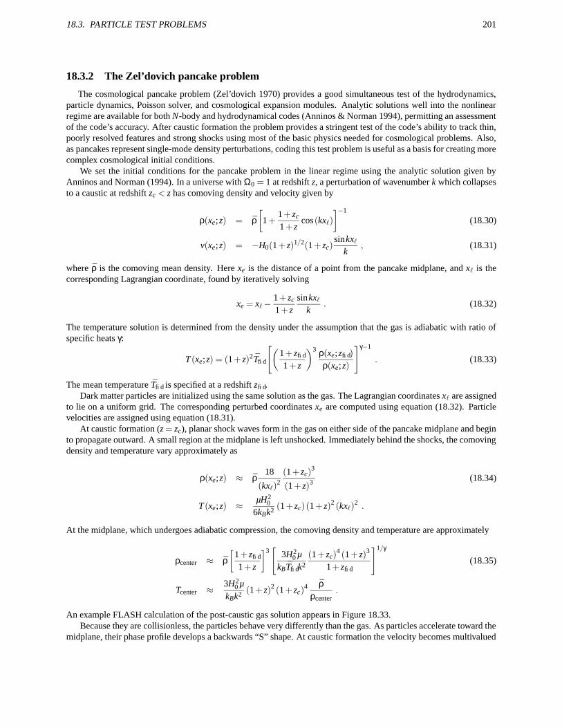
18.3. PARTICLE TEST PROBLEMS 201
18.3.2 The Zel’dovich pancake problem
The cosmological pancake problem (Zel’dovich 1970) provides a good simultaneous test of the hydrodynamics,particle dynamics, Poisson solver, and cosmological expansion modules. Analytic solutions well into the nonlinearregime are available for both N-body and hydrodynamical codes (Anninos & Norman 1994), permitting an assessmentof the code’s accuracy. After caustic formation the problem provides a stringent test of the code’s ability to track thin,poorly resolved features and strong shocks using most of the basic physics needed for cosmological problems. Also,as pancakes represent single-mode density perturbations, coding this test problem is useful as a basis for creating morecomplex cosmological initial conditions.
We set the initial conditions for the pancake problem in the linear regime using the analytic solution given byAnninos and Norman (1994). In a universe with Ω0 = 1 at redshift z, a perturbation of wavenumber k which collapsesto a caustic at redshift zc < z has comoving density and velocity given by
ρ(xe;z) = ρ[
1+1+ zc
1+ zcos(kx`)
]−1
(18.30)
v(xe;z) = −H0(1+ z)1/2(1+ zc)sinkx`
k, (18.31)
where ρ is the comoving mean density. Here xe is the distance of a point from the pancake midplane, and x` is thecorresponding Lagrangian coordinate, found by iteratively solving
xe = x`−1+ zc
1+ zsinkx`
k. (18.32)
The temperature solution is determined from the density under the assumption that the gas is adiabatic with ratio ofspecific heats γ:
T (xe;z) = (1+ z)2Tfid
[
(
1+ zfid
1+ z
)3 ρ(xe;zfid)
ρ(xe;z)
]γ−1
. (18.33)
The mean temperature Tfid is specified at a redshift zfid.Dark matter particles are initialized using the same solution as the gas. The Lagrangian coordinates x` are assigned
to lie on a uniform grid. The corresponding perturbed coordinates xe are computed using equation (18.32). Particlevelocities are assigned using equation (18.31).
At caustic formation (z = zc), planar shock waves form in the gas on either side of the pancake midplane and beginto propagate outward. A small region at the midplane is left unshocked. Immediately behind the shocks, the comovingdensity and temperature vary approximately as
ρ(xe;z) ≈ ρ18
(kx`)2
(1+ zc)3
(1+ z)3 (18.34)
T (xe;z) ≈ µH20
6kBk2 (1+ zc)(1+ z)2 (kx`)2 .
At the midplane, which undergoes adiabatic compression, the comoving density and temperature are approximately
ρcenter ≈ ρ[
1+ zfid
1+ z
]3[
3H20 µ
kBTfidk2
(1+ zc)4 (1+ z)3
1+ zfid
]1/γ
(18.35)
Tcenter ≈ 3H20 µ
kBk2 (1+ z)2 (1+ zc)4 ρ
ρcenter.
An example FLASH calculation of the post-caustic gas solution appears in Figure 18.33.Because they are collisionless, the particles behave very differently than the gas. As particles accelerate toward the
midplane, their phase profile develops a backwards “S” shape. At caustic formation the velocity becomes multivalued
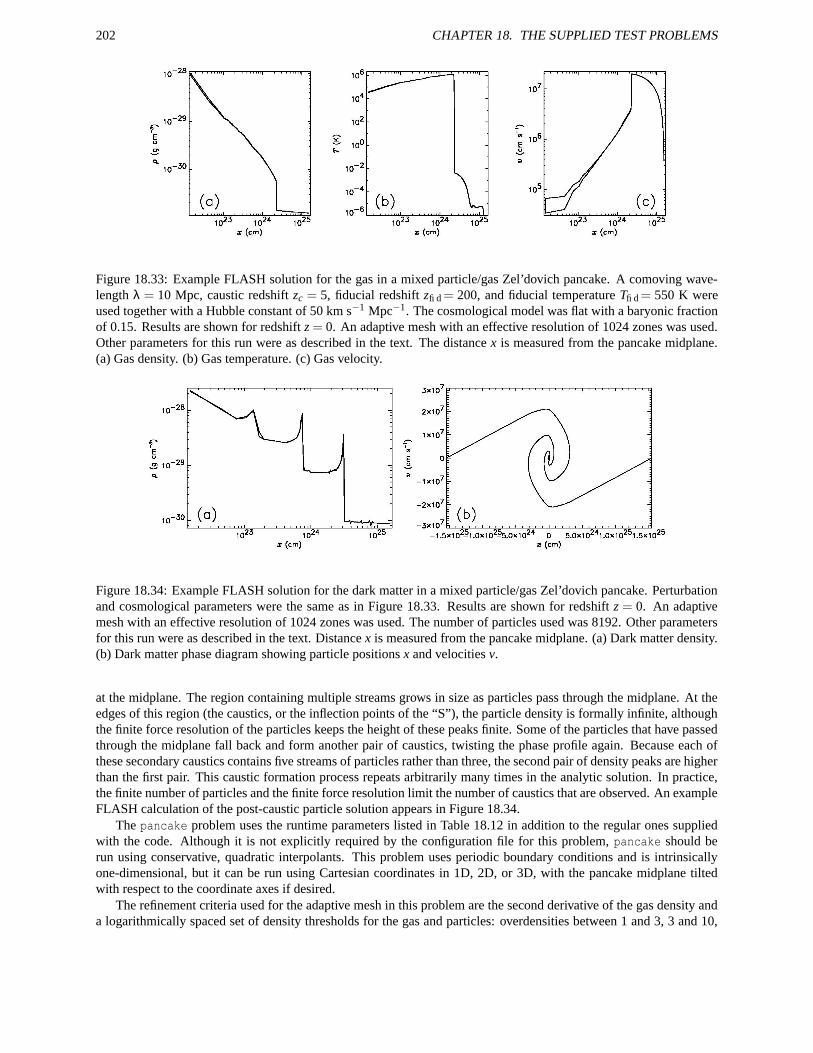
202 CHAPTER 18. THE SUPPLIED TEST PROBLEMS
Figure 18.33: Example FLASH solution for the gas in a mixed particle/gas Zel’dovich pancake. A comoving wave-length λ = 10 Mpc, caustic redshift zc = 5, fiducial redshift zfid = 200, and fiducial temperature Tfid = 550 K wereused together with a Hubble constant of 50 km s−1 Mpc−1. The cosmological model was flat with a baryonic fractionof 0.15. Results are shown for redshift z = 0. An adaptive mesh with an effective resolution of 1024 zones was used.Other parameters for this run were as described in the text. The distance x is measured from the pancake midplane.(a) Gas density. (b) Gas temperature. (c) Gas velocity.
Figure 18.34: Example FLASH solution for the dark matter in a mixed particle/gas Zel’dovich pancake. Perturbationand cosmological parameters were the same as in Figure 18.33. Results are shown for redshift z = 0. An adaptivemesh with an effective resolution of 1024 zones was used. The number of particles used was 8192. Other parametersfor this run were as described in the text. Distance x is measured from the pancake midplane. (a) Dark matter density.(b) Dark matter phase diagram showing particle positions x and velocities v.
at the midplane. The region containing multiple streams grows in size as particles pass through the midplane. At theedges of this region (the caustics, or the inflection points of the “S”), the particle density is formally infinite, althoughthe finite force resolution of the particles keeps the height of these peaks finite. Some of the particles that have passedthrough the midplane fall back and form another pair of caustics, twisting the phase profile again. Because each ofthese secondary caustics contains five streams of particles rather than three, the second pair of density peaks are higherthan the first pair. This caustic formation process repeats arbitrarily many times in the analytic solution. In practice,the finite number of particles and the finite force resolution limit the number of caustics that are observed. An exampleFLASH calculation of the post-caustic particle solution appears in Figure 18.34.
The pancake problem uses the runtime parameters listed in Table 18.12 in addition to the regular ones suppliedwith the code. Although it is not explicitly required by the configuration file for this problem, pancake should berun using conservative, quadratic interpolants. This problem uses periodic boundary conditions and is intrinsicallyone-dimensional, but it can be run using Cartesian coordinates in 1D, 2D, or 3D, with the pancake midplane tiltedwith respect to the coordinate axes if desired.
The refinement criteria used for the adaptive mesh in this problem are the second derivative of the gas density anda logarithmically spaced set of density thresholds for the gas and particles: overdensities between 1 and 3, 3 and 10,
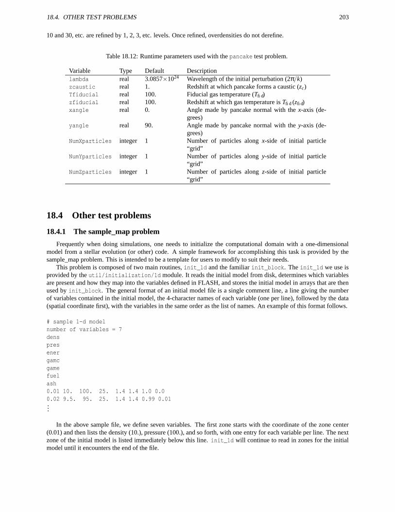
18.4. OTHER TEST PROBLEMS 203
10 and 30, etc. are refined by 1, 2, 3, etc. levels. Once refined, overdensities do not derefine.
Table 18.12: Runtime parameters used with the pancake test problem.
Variable Type Default Descriptionlambda real 3.0857×1024 Wavelength of the initial perturbation (2π/k)zcaustic real 1. Redshift at which pancake forms a caustic (zc)Tfiducial real 100. Fiducial gas temperature (Tfid)zfiducial real 100. Redshift at which gas temperature is Tfid (zfid)xangle real 0. Angle made by pancake normal with the x-axis (de-
grees)yangle real 90. Angle made by pancake normal with the y-axis (de-
grees)NumXparticles integer 1 Number of particles along x-side of initial particle
“grid”NumYparticles integer 1 Number of particles along y-side of initial particle
“grid”NumZparticles integer 1 Number of particles along z-side of initial particle
“grid”
18.4 Other test problems
18.4.1 The sample_map problem
Frequently when doing simulations, one needs to initialize the computational domain with a one-dimensionalmodel from a stellar evolution (or other) code. A simple framework for accomplishing this task is provided by thesample_map problem. This is intended to be a template for users to modify to suit their needs.
This problem is composed of two main routines, init_1d and the familiar init_block. The init_1d we use isprovided by the util/initialization/1d module. It reads the initial model from disk, determines which variablesare present and how they map into the variables defined in FLASH, and stores the initial model in arrays that are thenused by init_block. The general format of an initial model file is a single comment line, a line giving the numberof variables contained in the initial model, the 4-character names of each variable (one per line), followed by the data(spatial coordinate first), with the variables in the same order as the list of names. An example of this format follows.
# sample 1-d modelnumber of variables = 7denspresenergamcgamefuelash0.01 10. 100. 25. 1.4 1.4 1.0 0.00.02 9.5. 95. 25. 1.4 1.4 0.99 0.01...
In the above sample file, we define seven variables. The first zone starts with the coordinate of the zone center(0.01) and then lists the density (10.), pressure (100.), and so forth, with one entry for each variable per line. The nextzone of the initial model is listed immediately below this line. init_1d will continue to read in zones for the initialmodel until it encounters the end of the file.
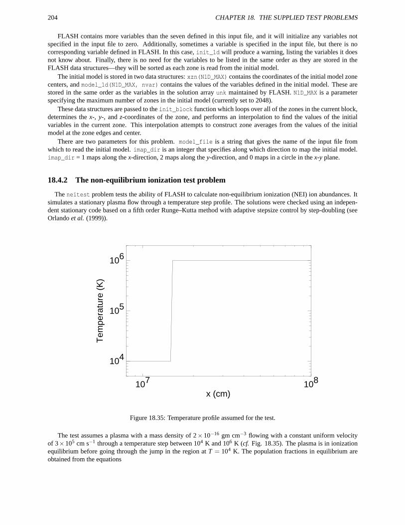
204 CHAPTER 18. THE SUPPLIED TEST PROBLEMS
FLASH contains more variables than the seven defined in this input file, and it will initialize any variables notspecified in the input file to zero. Additionally, sometimes a variable is specified in the input file, but there is nocorresponding variable defined in FLASH. In this case, init_1d will produce a warning, listing the variables it doesnot know about. Finally, there is no need for the variables to be listed in the same order as they are stored in theFLASH data structures—they will be sorted as each zone is read from the initial model.
The initial model is stored in two data structures: xzn(N1D_MAX) contains the coordinates of the initial model zonecenters, and model_1d(N1D_MAX, nvar) contains the values of the variables defined in the initial model. These arestored in the same order as the variables in the solution array unk maintained by FLASH. N1D_MAX is a parameterspecifying the maximum number of zones in the initial model (currently set to 2048).
These data structures are passed to the init_block function which loops over all of the zones in the current block,determines the x-, y-, and z-coordinates of the zone, and performs an interpolation to find the values of the initialvariables in the current zone. This interpolation attempts to construct zone averages from the values of the initialmodel at the zone edges and center.
There are two parameters for this problem. model_file is a string that gives the name of the input file fromwhich to read the initial model. imap_dir is an integer that specifies along which direction to map the initial model.imap_dir = 1 maps along the x-direction, 2 maps along the y-direction, and 0 maps in a circle in the x-y plane.
18.4.2 The non-equilibrium ionization test problem
The neitest problem tests the ability of FLASH to calculate non-equilibrium ionization (NEI) ion abundances. Itsimulates a stationary plasma flow through a temperature step profile. The solutions were checked using an indepen-dent stationary code based on a fifth order Runge–Kutta method with adaptive stepsize control by step-doubling (seeOrlando et al. (1999)).
107 108
x (cm)
104
105
106
Tem
pera
ture
(K
)
Figure 18.35: Temperature profile assumed for the test.
The test assumes a plasma with a mass density of 2× 10⁻¹⁶ gm cm−3 flowing with a constant uniform velocityof 3×105 cm s−1 through a temperature step between 104 K and 106 K (cf. Fig. 18.35). The plasma is in ionizationequilibrium before going through the jump in the region at T = 104 K. The population fractions in equilibrium areobtained from the equations
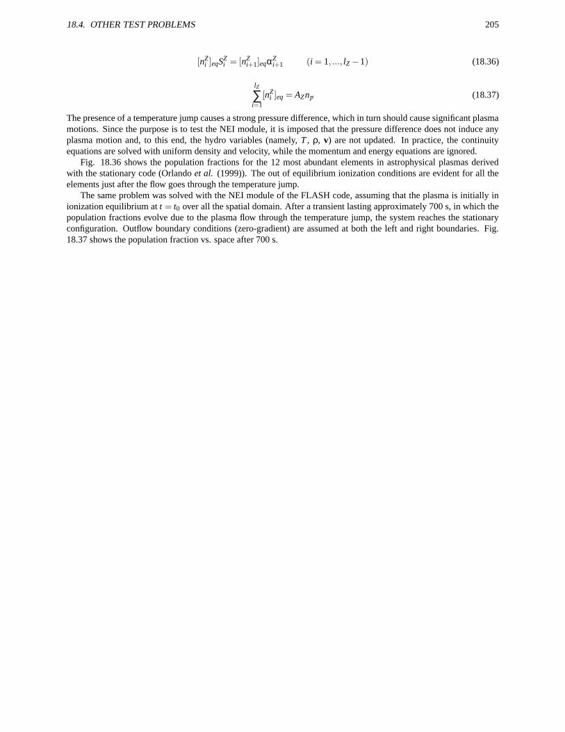
18.4. OTHER TEST PROBLEMS 205
[nZi ]eqSZ
i = [nZi+1]eqαZ
i+1 (i = 1, ..., lZ−1) (18.36)
lZ
∑i=1
[nZi ]eq = AZnp (18.37)
The presence of a temperature jump causes a strong pressure difference, which in turn should cause significant plasmamotions. Since the purpose is to test the NEI module, it is imposed that the pressure difference does not induce anyplasma motion and, to this end, the hydro variables (namely, T , ρ, v) are not updated. In practice, the continuityequations are solved with uniform density and velocity, while the momentum and energy equations are ignored.
Fig. 18.36 shows the population fractions for the 12 most abundant elements in astrophysical plasmas derivedwith the stationary code (Orlando et al. (1999)). The out of equilibrium ionization conditions are evident for all theelements just after the flow goes through the temperature jump.
The same problem was solved with the NEI module of the FLASH code, assuming that the plasma is initially inionization equilibrium at t = t0 over all the spatial domain. After a transient lasting approximately 700 s, in which thepopulation fractions evolve due to the plasma flow through the temperature jump, the system reaches the stationaryconfiguration. Outflow boundary conditions (zero-gradient) are assumed at both the left and right boundaries. Fig.18.37 shows the population fraction vs. space after 700 s.
206 CHAPTER 18. THE SUPPLIED TEST PROBLEMS
Population of He ions
107 108
x (cm)
10-5
10-4
10-3
10-2
10-1
100
Pop
ulat
ion
Fra
ctio
n
Population of C ions
107 108
x (cm)
10-5
10-4
10-3
10-2
10-1
100
Pop
ulat
ion
Fra
ctio
n
Population of N ions
107 108
x (cm)
10-5
10-4
10-3
10-2
10-1
100
Pop
ulat
ion
Fra
ctio
n
Population of O ions
107 108
x (cm)
10-5
10-4
10-3
10-2
10-1
100
Pop
ulat
ion
Fra
ctio
n
Population of Ne ions
107 108
x (cm)
10-5
10-4
10-3
10-2
10-1
100
Pop
ulat
ion
Fra
ctio
n
Population of Mg ions
107 108
x (cm)
10-5
10-4
10-3
10-2
10-1
100
Pop
ulat
ion
Fra
ctio
n
Figure 18.36: Numerical solutions of the stationary code. The figure shows the population fractions vs. space for the12 elements most abundant in astrophysical plasmas assuming a stationary flow through a temperature jump.
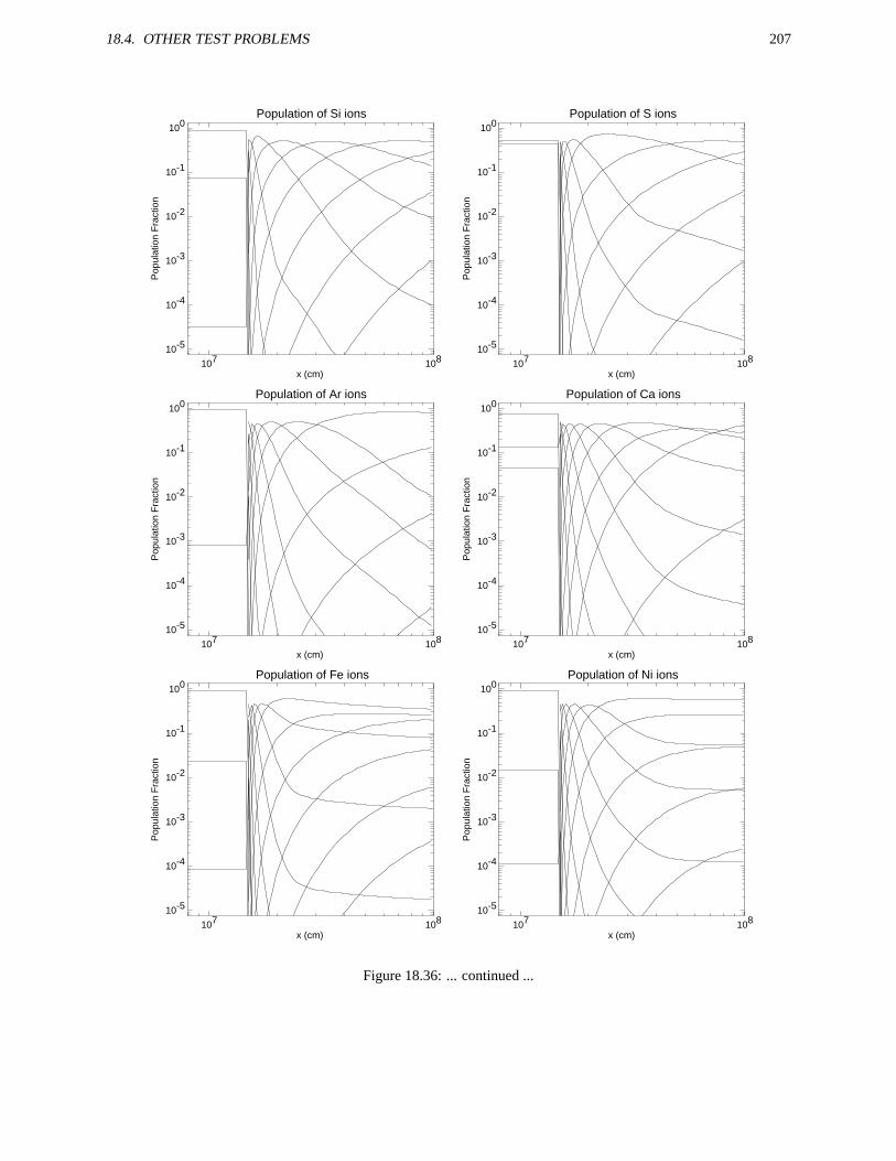
18.4. OTHER TEST PROBLEMS 207
Population of Si ions
107 108
x (cm)
10-5
10-4
10-3
10-2
10-1
100
Pop
ulat
ion
Fra
ctio
n
Population of S ions
107 108
x (cm)
10-5
10-4
10-3
10-2
10-1
100
Pop
ulat
ion
Fra
ctio
n
Population of Ar ions
107 108
x (cm)
10-5
10-4
10-3
10-2
10-1
100
Pop
ulat
ion
Fra
ctio
n
Population of Ca ions
107 108
x (cm)
10-5
10-4
10-3
10-2
10-1
100
Pop
ulat
ion
Fra
ctio
n
Population of Fe ions
107 108
x (cm)
10-5
10-4
10-3
10-2
10-1
100
Pop
ulat
ion
Fra
ctio
n
Population of Ni ions
107 108
x (cm)
10-5
10-4
10-3
10-2
10-1
100
Pop
ulat
ion
Fra
ctio
n
Figure 18.36: ... continued ...
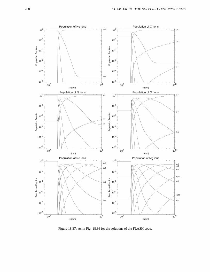
208 CHAPTER 18. THE SUPPLIED TEST PROBLEMS
Population of He ions
107 108
x (cm)
10-5
10-4
10-3
10-2
10-1
100
Pop
ulat
ion
Fra
ctio
n
He2
He3 Population of C ions
107 108
x (cm)
10-5
10-4
10-3
10-2
10-1
100
Pop
ulat
ion
Fra
ctio
n
C 4
C 5
C 6
C 7
Population of N ions
107 108
x (cm)
10-5
10-4
10-3
10-2
10-1
100
Pop
ulat
ion
Fra
ctio
n
N 5
N 6
N 7
Population of O ions
107 108
x (cm)
10-5
10-4
10-3
10-2
10-1
100
Pop
ulat
ion
Fra
ctio
n
O 5
O 6
O 7
O 8
Population of Ne ions
107 108
x (cm)
10-5
10-4
10-3
10-2
10-1
100
Pop
ulat
ion
Fra
ctio
n
Ne5
Ne6
Ne7
Ne8
Ne9
Population of Mg ions
107 108
x (cm)
10-5
10-4
10-3
10-2
10-1
100
Pop
ulat
ion
Fra
ctio
n
Mg5
Mg6
Mg7
Mg8Mg9
Mg10
Mg11
Figure 18.37: As in Fig. 18.36 for the solutions of the FLASH code.
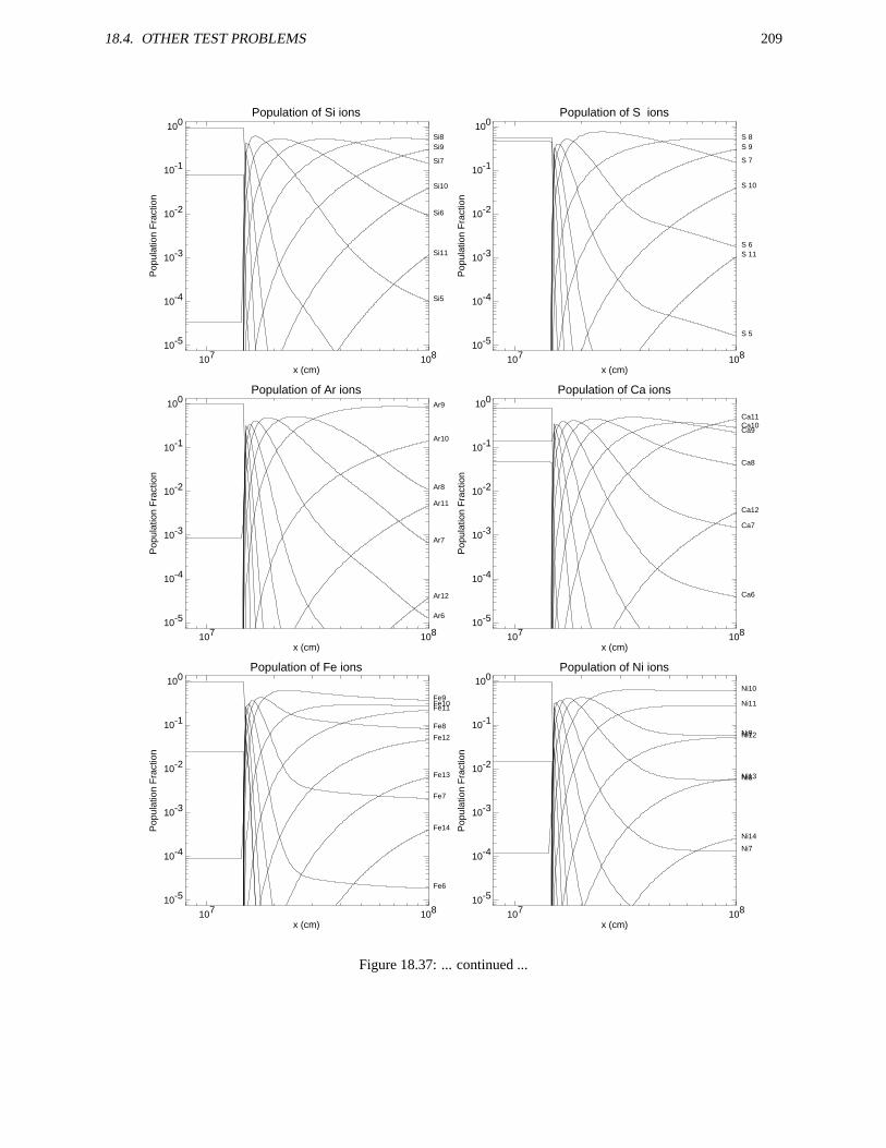
18.4. OTHER TEST PROBLEMS 209
Population of Si ions
107 108
x (cm)
10-5
10-4
10-3
10-2
10-1
100
Pop
ulat
ion
Fra
ctio
n
Si5
Si6
Si7
Si8Si9
Si10
Si11
Population of S ions
107 108
x (cm)
10-5
10-4
10-3
10-2
10-1
100
Pop
ulat
ion
Fra
ctio
n
S 5
S 6
S 7
S 8S 9
S 10
S 11
Population of Ar ions
107 108
x (cm)
10-5
10-4
10-3
10-2
10-1
100
Pop
ulat
ion
Fra
ctio
n
Ar6
Ar7
Ar8
Ar9
Ar10
Ar11
Ar12
Population of Ca ions
107 108
x (cm)
10-5
10-4
10-3
10-2
10-1
100
Pop
ulat
ion
Fra
ctio
n
Ca6
Ca7
Ca8
Ca9Ca10Ca11
Ca12
Population of Fe ions
107 108
x (cm)
10-5
10-4
10-3
10-2
10-1
100
Pop
ulat
ion
Fra
ctio
n
Fe6
Fe7
Fe8
Fe9Fe10Fe11
Fe12
Fe13
Fe14
Population of Ni ions
107 108
x (cm)
10-5
10-4
10-3
10-2
10-1
100
Pop
ulat
ion
Fra
ctio
n
Ni7
Ni8
Ni9
Ni10
Ni11
Ni12
Ni13
Ni14
Figure 18.37: ... continued ...

210 CHAPTER 18. THE SUPPLIED TEST PROBLEMS

Part IV
Tools
211

Chapter 19
Serial FLASH Output Comparison Utility(sfocu)
Sfocu (Serial Flash Output Comparison Utility) is mainly used as part of an automated testing suite calledflash_test and was introduced in FLASH version 2.0 as a replacement for focu.
Sfocu is a serial utility which examines two FLASH checkpoint files and decides whether or not they are “equal”to ensure that any changes made to FLASH do not adversely affect subsequent simulation output. By “equal”, wemean that
• The leaf-block structure matches – each leaf block must have the same position and size in both datasets.
• The data arrays in the leaf blocks (dens, pres...) are identical.
• The number of particles are the same, and all floating point particle attributes are identical.
Thus, sfocu ignores information such as the particular numbering of the blocks and particles, the timestamp, thebuild information, and so on.
Sfocu can read HDF4, HDF5, and PnetCDF FLASH checkpoint files. It has not been tested with FLASH checkpointsthat span multiple files. Although sfocu is a serial program, it is able to do comparisons on the output of large parallelsimulations. Sfocu has been used on irix, linux, AIX and OSF1.
19.1 Building sfocu
The process is entirely manual, although Makefiles for certain machines have been provided. There are a fewcompile-time options which you set via the following preprocessor definitions in the Makefile (in the CDEFINESmacro):
NO_HDF4 build without HDF4 support
NO_HDF5 build without HDF5 support
NO_NCDF build without PnetCDF support
NEED_MPI certain parallel versions of HDF5 and all versions of PnetCDF need to be linked with the MPI library. Thisadds the necessary MPI_Init and MPI_Finalize calls to sfocu. There is no advantage to running sfocu onmore than one processor; it will only give you multiple copies of the same report.
19.2 Using sfocu
There are no command line options. Simply run the command sfocu <file1> <file2>. You will most likelyneed to widen your terminal to view the output, since it is well over 80 columns. Sample output follows:
213

214 CHAPTER 19. SERIAL FLASH OUTPUT COMPARISON UTILITY (SFOCU)
sfocu: comparing advect_2d_45deg_sqr_4lev_hdf_chk_0002 and advect_2d_45deg_gau_4lev_hdf_chk_0002
Min Error: inf(2|a-b| / max(|a+b|, 1e-99) )Max Error: sup(2|a-b| / max(|a+b|, 1e-99) )Abs Error: sup|a-b|Mag Error: sup|a-b| / max(sup|a|, sup|b|, 1e-99)
advect_2d_45deg_sqr_4lev_hdf_chk_0002 has 2 leaf blocks that don’t exist in advect_2d_45deg_gau_4lev_hdf_chk_0002advect_2d_45deg_gau_4lev_hdf_chk_0002 has 8 leaf blocks that don’t exist in advect_2d_45deg_sqr_4lev_hdf_chk_0002Total leaf blocks compared: 53 (all other blocks are ignored)-----+------------+-----------+-----------+-----------+-----------++-----------+-----------+-----------++-----------+-----------+-----------+Var | Bad Blocks | Min Error | Max Error | Abs Error | Mag Error || Sum | Max | Min || Sum | Max | Min |-----+------------+-----------+-----------+-----------+-----------++-----------+-----------+-----------++-----------+-----------+-----------+pres | 53 | 1.11e-16 | 3.234e-13 | 3.234e-13 | 3.234e-13 || 3.39e+03 | 1 | 1 || 3.39e+03 | 1 | 1 |gamc | 0 | 0 | 0 | 0 | 0 || 4.75e+03 | 1.4 | 1.4 || 4.75e+03 | 1.4 | 1.4 |game | 0 | 0 | 0 | 0 | 0 || 4.75e+03 | 1.4 | 1.4 || 4.75e+03 | 1.4 | 1.4 |dens | 53 | 1.694e-16 | 1.998 | 0.6311 | 0.6311 || 714 | 1 | 1e-05 || 619 | 0.958 | 1e-05 |velx | 53 | 1.256e-16 | 2.373e-13 | 1.678e-12 | 2.373e-13 || 2.4e+04 | 7.07 | 7.07 || 2.4e+04 | 7.07 | 7.07 |temp | 53 | 1.803e-16 | 1.998 | 0.001194 | 0.9932 || 2.43 | 0.0012 | 1.2e-08 || 1.5 | 0.0012 | 1.26e-08 |velz | 0 | 0 | 0 | 0 | 0 || 0 | 0 | 0 || 0 | 0 | 0 |ener | 53 | 1.164e-16 | 1.997 | 2.483e+05 | 0.993 || 5.05e+08 | 2.5e+05 | 52.5 || 3.12e+08 | 2.5e+05 | 52.6 |vely | 53 | 1.256e-16 | 2.007e-13 | 1.419e-12 | 2.007e-13 || 2.4e+04 | 7.07 | 7.07 || 2.4e+04 | 7.07 | 7.07 |1 | 53 | 1.11e-16 | 2.499e-09 | 2.499e-09 | 2.499e-09 || 3.39e+03 | 1 | 1 || 3.39e+03 | 1 | 1 |
-----+------------+-----------+-----------+-----------+-----------++-----------+-----------+-----------++-----------+-----------+-----------+FAILURE
“Bad Blocks” is the number of leaf blocks where the data was found to differ between datasets. Four differenterror measures (min/max/abs/mag) are defined in the output above. In addition, the last six columns report the sum,maximum and minimum of the variables in the two files. Note that the sum is physically meaningless, since it is notvolume-weighted. Finally, the last line permits other programs to parse the sfocu output easily: when the files areidentical, the line will instead read SUCCESS.
It is possible for sfocu to miss machine-precision variations in the data on certain machines because of compileror library issues, although this has only been observed on one platform, where the compiler produced code that ignoredIEEE rules until the right flag was found.
Chapter 20
FLASH IDL routines (fidlr)
fidlr is a set of routines written in IDL that can read and plot data files produced by FLASH. These routines includeprograms which can be run from the IDL command line to read 1D, 2D, or 3D FLASH datasets, interactively analyzedatasets, and interpolate them onto uniform grids. A graphical interface to these routines (xflash) is provided, whichenables users to read FLASH AMR datasets or global integral files (flash.dat) and make plots and histograms ofthe data. There are two sets of routines, fidlr2 that do not directly support the HDF5 data format, and fidlr3 thatdo. In terms of their functionality they are very similar. The difference is that fidlr3 routines need IDL version 5.6and above; the earlier versions did not support HDF5 data format. The routines in fidlr2 can work with any versionof IDL, since they do not assume HDF5 data format support. They use call_external function to interface witha set of C routines that read in the HDF5 data (see Chapter 7). Using these routines requires that the HDF5 librarybe installed on your system and that the shared-object wrapper library be compiled before reading in data. Since thecall_external function is used, the demo version of IDL will not run the routines.
The fidlr routines support 1-, 2-, and 3-dimensional datasets in the FLASH HDF5 formats. Both plotfiles andcheckpoint files, which differ only in the number and numerical precision of the variables stored, are supported.Additionally, 1-d plots from the flash.dat files can be made as well. The following sections assume that the user hassome familiarity with IDL. The examples discussed below will use the Sedov data generated in the quickstart at thebeginning of this manual.
20.1 Installing and running fidlr2
fidlr2 is distributed with FLASH and is contained in the tools/fidlr2/ directory. In addition to the IDL proce-dures, a README file is present which will contain up-to-date information on changes and installation requirements.
These routines were written and tested using IDL v5.4 for Linux. They should work without difficulty on any UNIXmachine with IDL installed—any functionality of fidlr2 under Windows is purely coincidental. Later versions ofIDL no longer support GIF files due to copyright difficulties, so PNG images will be produced in their place. Mostgraphics packages, like xv or the GIMP, should be able to convert between these formats. It is possible to run IDL in a‘demo’ mode if there are not enough licenses available. Unfortunately, some parts of fidlr2 will not function in thismode, since certain features of IDL are disabled. In particular, the call_external function is disabled, making theHDF5 wrappers inoperable. This guide assumes that you are running the full version of IDL.
Installation of fidlr2 requires defining some environment variables, making sure your IDL path is properly set,and compiling the support for HDF5 files. These procedures are described below.
20.1.1 Setting up fidlr2 environment variables
The FLASH fidlr2 routines are located in the tools/fidlr2/ subdirectory of the FLASH root directory. To usethem you must set two environment variables. First set the value of XFLASH_DIR to the location of the FLASH IDLroutines; for example, under csh, use
setenv XFLASH_DIR flash-root-path/tools/fidlr2 ,
215
216 CHAPTER 20. FLASH IDL ROUTINES (FIDLR)
where flash-root-path is the absolute path of the FLASH root directory. This variable is used in the plotting routines tofind the customized color table for xflash, as well as to identify the location of the shared-object libraries compiledfor HDF5 support.
Next, make sure that you have an IDL_DIR environment variable set. This should point to the directory in whichthe IDL distribution is installed. For example, if IDL is installed in idl-root-path, then you would define
setenv IDL_DIR idl-root-path .
Finally, you need to tell IDL where to find the fidlr2 routines. This is accomplished through the IDL_PATHenvironment variable
setenv IDL_PATH $XFLASH_DIR:$IDL_DIR:$IDL_DIR/lib .
If you already have an IDL_PATH environment variable defined, just add XFLASH_DIR to the beginning of it. You maywish to include these commands in your .cshrc (or the analogous versions in your .profile file, depending on yourshell) to avoid having to reissue them every time you log in. It is important that the $XFLASH_DIR come beforethe IDL directories in the path and that the $IDL_DIR/lib directory be included as well (otherwise, the compoundwidget procedures, cw_*.pro, will not be found).
20.1.2 Setting up the HDF5 routines
For fidlr2 to read HDF5 files, you need to install the HDF5 library on your machine and compile the wrap-per routines. The HDF5 libraries can be obtained in either source or binary form for most Unix platforms fromhttp://hdf.ncsa.uiuc.edu. Two sample Makefiles are provided. Makefile.sgi will build the shared-object li-brary on an SGI. Makefile.linux will build the library on a Linux machine. In both cases, the Makefile will need tobe edited to point to the directories where IDL and HDF5 are installed on the local machine. The compiler flags for ashared-object library for different versions of Unix can be found in
$IDL_DIR/external/call_external/C/callext_unix.txt .
for IDL versions ≤ 5.5, and by typing
print, !MAKE_DLL
at the IDL prompt for IDL 5.6.The compilation flags in the Makefile should be modified according to the instructions in that file or the output of
the !MAKE_DLL IDL system variable. Again, the path to the HDF5 library needs to be supplied so the header files canbe used in the compilation process, and for the linking stage. The path to the IDL header export.h is needed as well,to deal with IDL strings. IDL defines strings as structures, with a field of the IDL_STRING structure giving the lengthof the string. The datatype of this field has changed from version to version, so we need to get the actual definitionfrom the IDL header files.
It is important that you compile the shared-object to conform to the same application binary interface (ABI) thatIDL was compiled with. This is mainly an issue on an SGI, where IDL version 5.2.1 and later use the n32 ABI, whileversions before this are o32. The HDF library will also need to be compiled in the same format. You can check theformat of the HDF5 library and your version of IDL with the UNIX file command.
IDL interacts with external programs through the call_external function. Any arguments are passed by refer-ence through the standard C command line argument interface, argc and argv. These are recast into pointers of theproper type in the C routines. The C wrappers call the appropriate HDF functions to read the data and return it throughthe argc pointers.
Finally, if the HDF5 library was installed as a shared-object, then the library must be in your shell’s library searchpath. This can be set by defining the LD_LIBRARY_PATH environment variable to point to the HDF5 lib/ subdirectory.
20.1.3 Running IDL
fidlr2 uses 8-bit color tables for all of its plotting. On displays with higher color depths, it may be necessary to usecolor overlays to get the proper colors on your display. For SGI machines, launching IDL with the start.pro scriptwill enable 8-bit pseudocolor overlays. For Linux boxes, setting the X color depth to 24-bits per pixel and launchingIDL with the start_linux.pro script usually produces proper colors.
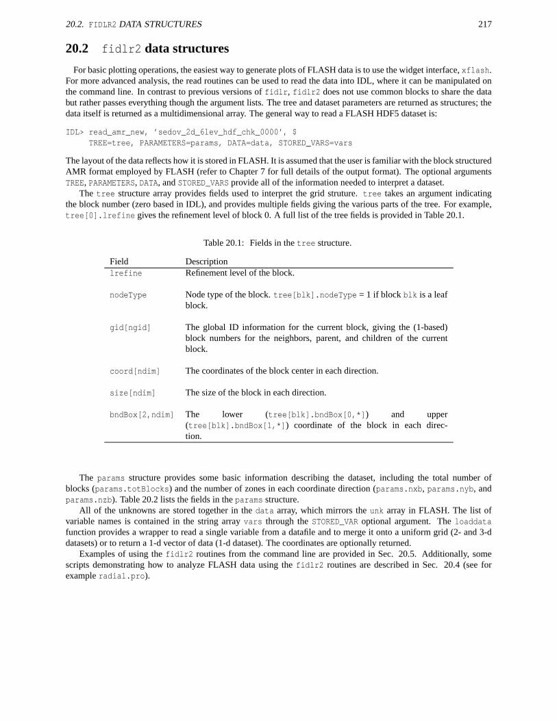
20.2. FIDLR2 DATA STRUCTURES 217
20.2 fidlr2 data structures
For basic plotting operations, the easiest way to generate plots of FLASH data is to use the widget interface, xflash.For more advanced analysis, the read routines can be used to read the data into IDL, where it can be manipulated onthe command line. In contrast to previous versions of fidlr, fidlr2 does not use common blocks to share the databut rather passes everything though the argument lists. The tree and dataset parameters are returned as structures; thedata itself is returned as a multidimensional array. The general way to read a FLASH HDF5 dataset is:
IDL> read_amr_new, ’sedov_2d_6lev_hdf_chk_0000’, $TREE=tree, PARAMETERS=params, DATA=data, STORED_VARS=vars
The layout of the data reflects how it is stored in FLASH. It is assumed that the user is familiar with the block structuredAMR format employed by FLASH (refer to Chapter 7 for full details of the output format). The optional argumentsTREE, PARAMETERS, DATA, and STORED_VARS provide all of the information needed to interpret a dataset.
The tree structure array provides fields used to interpret the grid struture. tree takes an argument indicatingthe block number (zero based in IDL), and provides multiple fields giving the various parts of the tree. For example,tree[0].lrefine gives the refinement level of block 0. A full list of the tree fields is provided in Table 20.1.
Table 20.1: Fields in the tree structure.
Field Descriptionlrefine Refinement level of the block.
nodeType Node type of the block. tree[blk].nodeType = 1 if block blk is a leafblock.
gid[ngid] The global ID information for the current block, giving the (1-based)block numbers for the neighbors, parent, and children of the currentblock.
coord[ndim] The coordinates of the block center in each direction.
size[ndim] The size of the block in each direction.
bndBox[2,ndim] The lower (tree[blk].bndBox[0,*]) and upper(tree[blk].bndBox[1,*]) coordinate of the block in each direc-tion.
The params structure provides some basic information describing the dataset, including the total number ofblocks (params.totBlocks) and the number of zones in each coordinate direction (params.nxb, params.nyb, andparams.nzb). Table 20.2 lists the fields in the params structure.
All of the unknowns are stored together in the data array, which mirrors the unk array in FLASH. The list ofvariable names is contained in the string array vars through the STORED_VAR optional argument. The loaddatafunction provides a wrapper to read a single variable from a datafile and to merge it onto a uniform grid (2- and 3-ddatasets) or to return a 1-d vector of data (1-d dataset). The coordinates are optionally returned.
Examples of using the fidlr2 routines from the command line are provided in Sec. 20.5. Additionally, somescripts demonstrating how to analyze FLASH data using the fidlr2 routines are described in Sec. 20.4 (see forexample radial.pro).
218 CHAPTER 20. FLASH IDL ROUTINES (FIDLR)
Table 20.2: Fields in the params structure.
Field DescriptiontotBlocks The total number of blocks in the dataset.
corners A logical variable specifying whether the data was interpolated to cornersbefore storage.
ndim The number of dimensions of the simulation.
nxb The number of zones per block in the x-direction.
nyb The number of zones per block in the y-direction.
nzb The number of zones per block in the z-direction.
ntopx The number of top level blocks in the x-direction. This is equal to theNblocksx FLASH runtime parameter.
ntopy The number of top level blocks in the y-direction. This is equal to theNblocksy FLASH runtime parameter.
ntopz The number of top level blocks in the z-direction. This is equal to theNblocksz FLASH runtime parameter.
time The simulation time of the current dataset.
dt The timestep used for the last step.
The driver routines provided with fidlr2 visualize the AMR data by first converting it to a uniform mesh. Thisallows for ease of plotting and manipulation, including contour plotting, but it is less efficient than plotting the nativeAMR structure. Efficiency is gained by recognizing that the data is restricted up the tree before output, so it is validat all levels. If the dataset is much larger than the plot device, we ignore those levels that are finer than the deviceresolution and produce the plot using blocks closer to the root of the tree. In 3-d, slices through the dataset are madeby putting only the 2-d slice itself onto a uniform grid. Analysis can still be performed directly on the native datathrough the command line.
20.3 xflash: widget interface to plotting FLASH datasets
The main interface to the fidlr2 routines for plotting FLASH datasets is xflash. Typing xflash at the IDLcommand prompt will launch the main xflash widget, shown in Fig. 20.1. xflash produces colormap plots ofFLASH data with optional overlays of velocity vectors, contours, and the AMR block structure and histogram plotsshowing the distribution of data. The basic operation of xflash is to specify a single file in the dataset as a prototypefor the FLASH simulation. The prototype is probed for the list of variables it contains, and then the remaining plotoptions become active.
xflash can output to the screen, postscript, or an image file (GIF/PNG). If the data is significantly higher reso-lution than the output device, xflash (through xplot_amr.pro) will sub-sample the image by one or more levels ofrefinement before plotting.
Once the image is plotted, the query (2-d data only) and 1-d slice (1 and 2-d data only) buttons will becomeactive. Pressing query and then clicking anywhere in the domain will pop up a window containing the values ofall the FLASH variables in the zone nearest the cursor. The query function uses the actual FLASH data—not theinterpolated/uniformly gridded data generated for the plots. Pressing 1-d slice and then left-clicking on the plot will
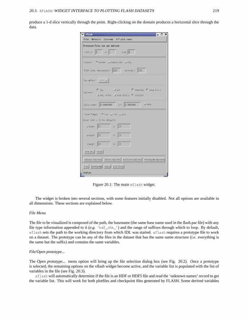
20.3. XFLASH: WIDGET INTERFACE TO PLOTTING FLASH DATASETS 219
produce a 1-d slice vertically through the point. Right-clicking on the domain produces a horizontal slice through thedata.
Figure 20.1: The main xflash widget.
The widget is broken into several sections, with some features initially disabled. Not all options are available inall dimensions. These sections are explained below.
File Menu
The file to be visualized is composed of the path, the basename (the same base name used in the flash.par file) with anyfile type information appended to it (e.g. ’hdf_chk_’) and the range of suffixes through which to loop. By default,xflash sets the path to the working directory from which IDL was started. xflash requires a prototype file to workon a dataset. The prototype can be any of the files in the dataset that has the same name structure (i.e. everything isthe same but the suffix) and contains the same variables.
File/Open prototype...
The Open prototype... menu option will bring up the file selection dialog box (see Fig. 20.2). Once a prototypeis selected, the remaining options on the xflash widget become active, and the variable list is populated with the list ofvariables in the file (see Fig. 20.3).
xflash will automatically determine if the file is an HDF or HDF5 file and read the ‘unknown names’ record to getthe variable list. This will work for both plotfiles and checkpoint files generated by FLASH. Some derived variables
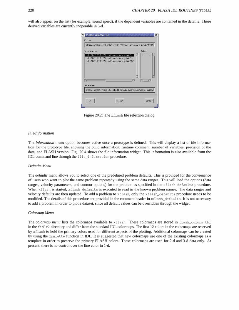
220 CHAPTER 20. FLASH IDL ROUTINES (FIDLR)
will also appear on the list (for example, sound speed), if the dependent variables are contained in the datafile. Thesederived variables are currently inoperable in 3-d.
Figure 20.2: The xflash file selection dialog.
File/Information
The Information menu option becomes active once a prototype is defined. This will display a list of file informa-tion for the prototype file, showing the build information, runtime comment, number of variables, precision of thedata, and FLASH version. Fig. 20.4 shows the file information widget. This information is also available from theIDL command line through the file_information procedure.
Defaults Menu
The defaults menu allows you to select one of the predefined problem defaults. This is provided for the convienenceof users who want to plot the same problem repeatedy using the same data ranges. This will load the options (dataranges, velocity parameters, and contour options) for the problem as specified in the xflash_defaults procedure.When xflash is started, xflash_defaults is executed to read in the known problem names. The data ranges andvelocity defaults are then updated. To add a problem to xflash, only the xflash_defaults procedure needs to bemodified. The details of this procedure are provided in the comment header in xflash_defaults. It is not necessaryto add a problem in order to plot a dataset, since all default values can be overridden through the widget.
Colormap Menu
The colormap menu lists the colormaps available to xflash. These colormaps are stored in flash_colors.tblin the fidlr2 directory and differ from the standard IDL colormaps. The first 12 colors in the colormaps are reservedby xflash to hold the primary colors used for different aspects of the plotting. Additional colormaps can be createdby using the xpalette function in IDL. It is suggested that new colormaps use one of the existing colormaps as atemplate in order to preserve the primary FLASH colors. These colormaps are used for 2-d and 3-d data only. Atpresent, there is no control over the line color in 1-d.
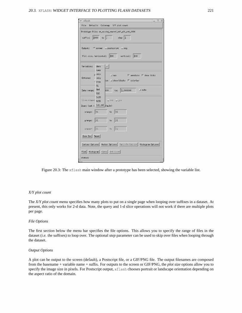
20.3. XFLASH: WIDGET INTERFACE TO PLOTTING FLASH DATASETS 221
Figure 20.3: The xflash main window after a prototype has been selected, showing the variable list.
X/Y plot count
The X/Y plot count menu specifies how many plots to put on a single page when looping over suffixes in a dataset. Atpresent, this only works for 2-d data. Note, the query and 1-d slice operations will not work if there are multiple plotsper page.
File Options
The first section below the menu bar specifies the file options. This allows you to specify the range of files in thedataset (i.e. the suffixes) to loop over. The optional step parameter can be used to skip over files when looping throughthe dataset.
Output Options
A plot can be output to the screen (default), a Postscript file, or a GIF/PNG file. The output filenames are composedfrom the basename + variable name + suffix. For outputs to the screen or GIF/PNG, the plot size options allow you tospecify the image size in pixels. For Postscript output, xflash chooses portrait or landscape orientation depending onthe aspect ratio of the domain.
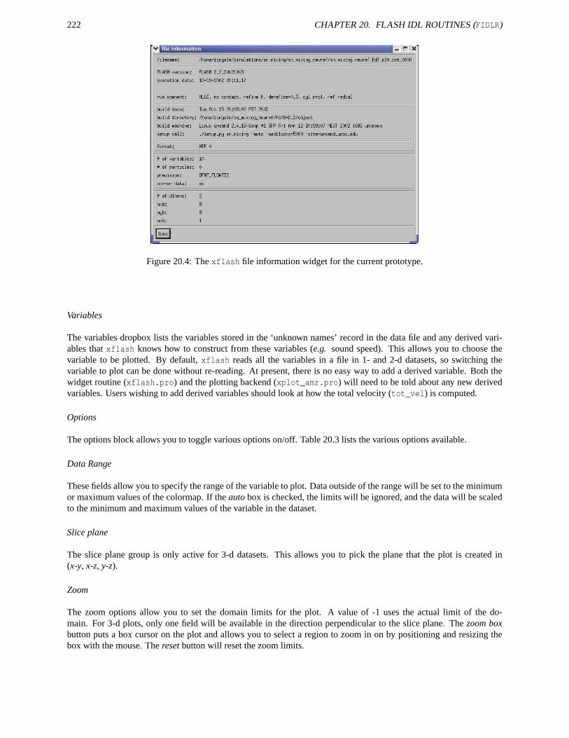
222 CHAPTER 20. FLASH IDL ROUTINES (FIDLR)
Figure 20.4: The xflash file information widget for the current prototype.
Variables
The variables dropbox lists the variables stored in the ‘unknown names’ record in the data file and any derived vari-ables that xflash knows how to construct from these variables (e.g. sound speed). This allows you to choose thevariable to be plotted. By default, xflash reads all the variables in a file in 1- and 2-d datasets, so switching thevariable to plot can be done without re-reading. At present, there is no easy way to add a derived variable. Both thewidget routine (xflash.pro) and the plotting backend (xplot_amr.pro) will need to be told about any new derivedvariables. Users wishing to add derived variables should look at how the total velocity (tot_vel) is computed.
Options
The options block allows you to toggle various options on/off. Table 20.3 lists the various options available.
Data Range
These fields allow you to specify the range of the variable to plot. Data outside of the range will be set to the minimumor maximum values of the colormap. If the auto box is checked, the limits will be ignored, and the data will be scaledto the minimum and maximum values of the variable in the dataset.
Slice plane
The slice plane group is only active for 3-d datasets. This allows you to pick the plane that the plot is created in(x-y, x-z, y-z).
Zoom
The zoom options allow you to set the domain limits for the plot. A value of -1 uses the actual limit of the do-main. For 3-d plots, only one field will be available in the direction perpendicular to the slice plane. The zoom boxbutton puts a box cursor on the plot and allows you to select a region to zoom in on by positioning and resizing thebox with the mouse. The reset button will reset the zoom limits.
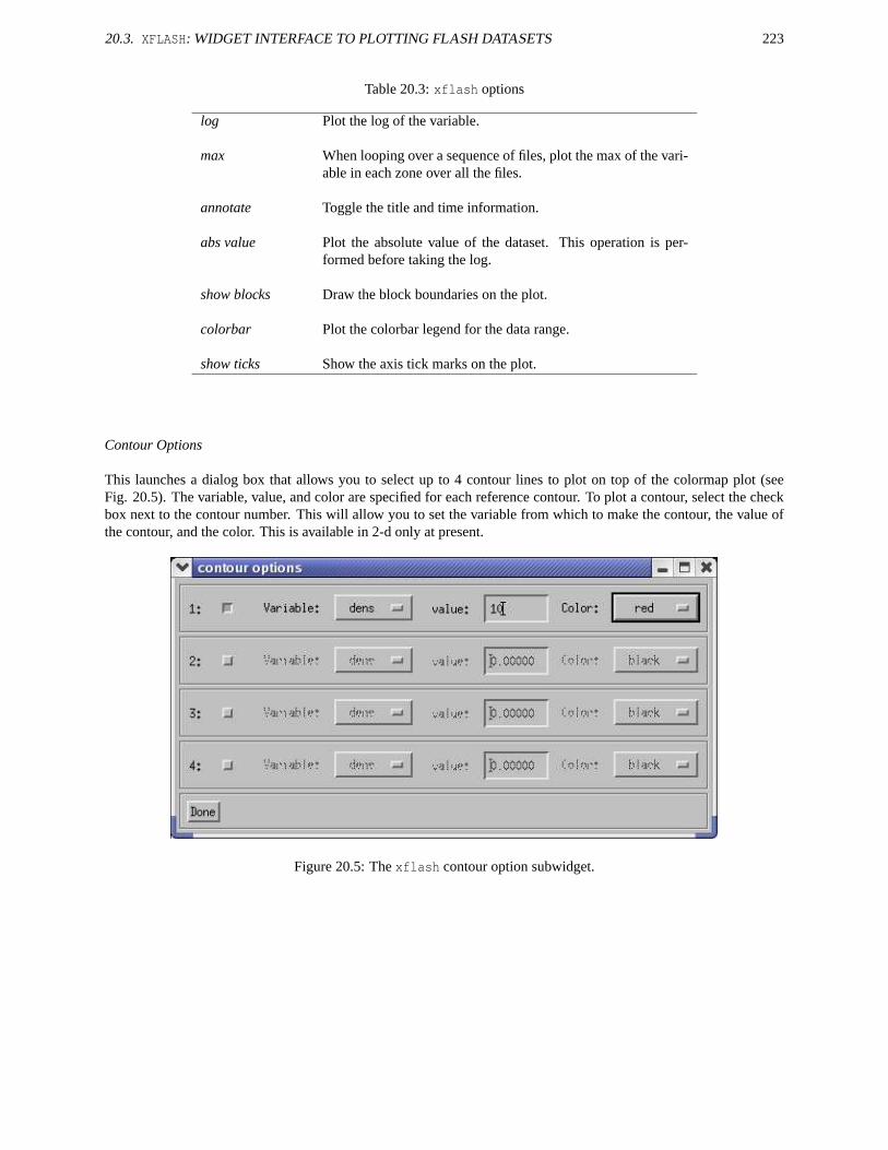
20.3. XFLASH: WIDGET INTERFACE TO PLOTTING FLASH DATASETS 223
Table 20.3: xflash options
log Plot the log of the variable.
max When looping over a sequence of files, plot the max of the vari-able in each zone over all the files.
annotate Toggle the title and time information.
abs value Plot the absolute value of the dataset. This operation is per-formed before taking the log.
show blocks Draw the block boundaries on the plot.
colorbar Plot the colorbar legend for the data range.
show ticks Show the axis tick marks on the plot.
Contour Options
This launches a dialog box that allows you to select up to 4 contour lines to plot on top of the colormap plot (seeFig. 20.5). The variable, value, and color are specified for each reference contour. To plot a contour, select the checkbox next to the contour number. This will allow you to set the variable from which to make the contour, the value ofthe contour, and the color. This is available in 2-d only at present.
Figure 20.5: The xflash contour option subwidget.
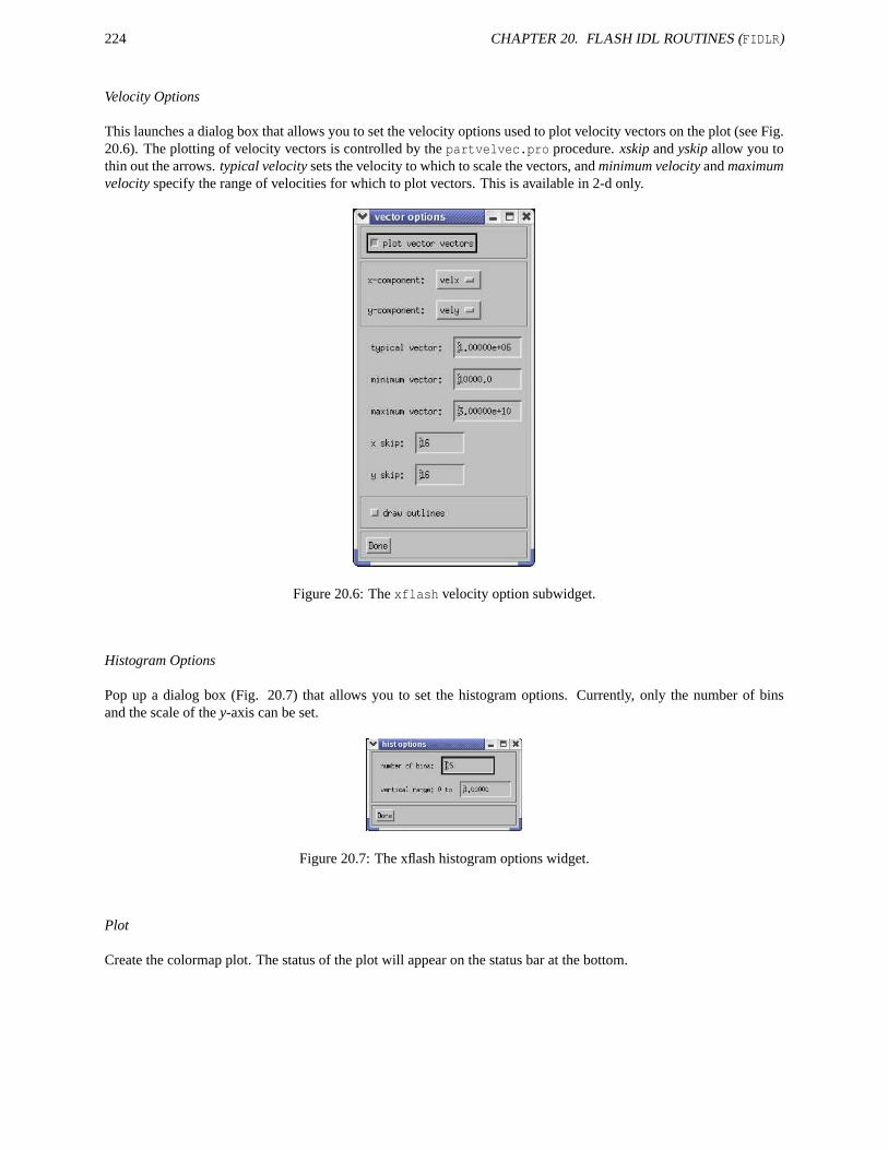
224 CHAPTER 20. FLASH IDL ROUTINES (FIDLR)
Velocity Options
This launches a dialog box that allows you to set the velocity options used to plot velocity vectors on the plot (see Fig.20.6). The plotting of velocity vectors is controlled by the partvelvec.pro procedure. xskip and yskip allow you tothin out the arrows. typical velocity sets the velocity to which to scale the vectors, and minimum velocity and maximumvelocity specify the range of velocities for which to plot vectors. This is available in 2-d only.
Figure 20.6: The xflash velocity option subwidget.
Histogram Options
Pop up a dialog box (Fig. 20.7) that allows you to set the histogram options. Currently, only the number of binsand the scale of the y-axis can be set.
Figure 20.7: The xflash histogram options widget.
Plot
Create the colormap plot. The status of the plot will appear on the status bar at the bottom.
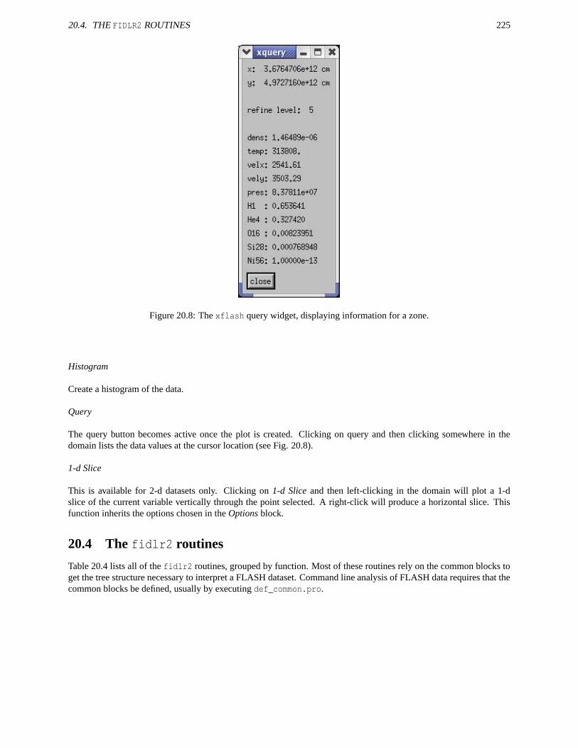
20.4. THE FIDLR2 ROUTINES 225
Figure 20.8: The xflash query widget, displaying information for a zone.
Histogram
Create a histogram of the data.
Query
The query button becomes active once the plot is created. Clicking on query and then clicking somewhere in thedomain lists the data values at the cursor location (see Fig. 20.8).
1-d Slice
This is available for 2-d datasets only. Clicking on 1-d Slice and then left-clicking in the domain will plot a 1-dslice of the current variable vertically through the point selected. A right-click will produce a horizontal slice. Thisfunction inherits the options chosen in the Options block.
20.4 The fidlr2 routines
Table 20.4 lists all of the fidlr2 routines, grouped by function. Most of these routines rely on the common blocks toget the tree structure necessary to interpret a FLASH dataset. Command line analysis of FLASH data requires that thecommon blocks be defined, usually by executing def_common.pro.
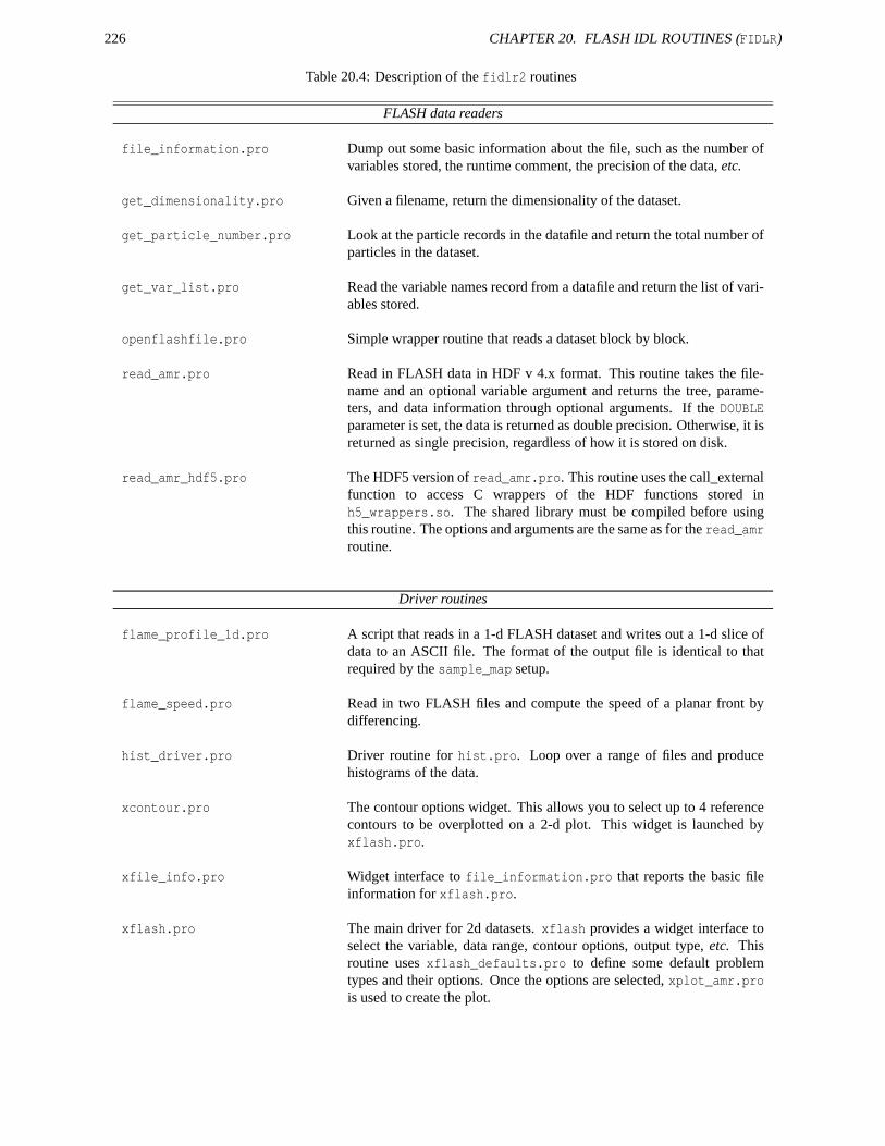
226 CHAPTER 20. FLASH IDL ROUTINES (FIDLR)
Table 20.4: Description of the fidlr2 routines
FLASH data readers
file_information.pro Dump out some basic information about the file, such as the number ofvariables stored, the runtime comment, the precision of the data, etc.
get_dimensionality.pro Given a filename, return the dimensionality of the dataset.
get_particle_number.pro Look at the particle records in the datafile and return the total number ofparticles in the dataset.
get_var_list.pro Read the variable names record from a datafile and return the list of vari-ables stored.
openflashfile.pro Simple wrapper routine that reads a dataset block by block.
read_amr.pro Read in FLASH data in HDF v 4.x format. This routine takes the file-name and an optional variable argument and returns the tree, parame-ters, and data information through optional arguments. If the DOUBLEparameter is set, the data is returned as double precision. Otherwise, it isreturned as single precision, regardless of how it is stored on disk.
read_amr_hdf5.pro The HDF5 version of read_amr.pro. This routine uses the call_externalfunction to access C wrappers of the HDF functions stored inh5_wrappers.so. The shared library must be compiled before usingthis routine. The options and arguments are the same as for the read_amrroutine.
Driver routines
flame_profile_1d.pro A script that reads in a 1-d FLASH dataset and writes out a 1-d slice ofdata to an ASCII file. The format of the output file is identical to thatrequired by the sample_map setup.
flame_speed.pro Read in two FLASH files and compute the speed of a planar front bydifferencing.
hist_driver.pro Driver routine for hist.pro. Loop over a range of files and producehistograms of the data.
xcontour.pro The contour options widget. This allows you to select up to 4 referencecontours to be overplotted on a 2-d plot. This widget is launched byxflash.pro.
xfile_info.pro Widget interface to file_information.pro that reports the basic fileinformation for xflash.pro.
xflash.pro The main driver for 2d datasets. xflash provides a widget interface toselect the variable, data range, contour options, output type, etc. Thisroutine uses xflash_defaults.pro to define some default problemtypes and their options. Once the options are selected, xplot_amr.prois used to create the plot.
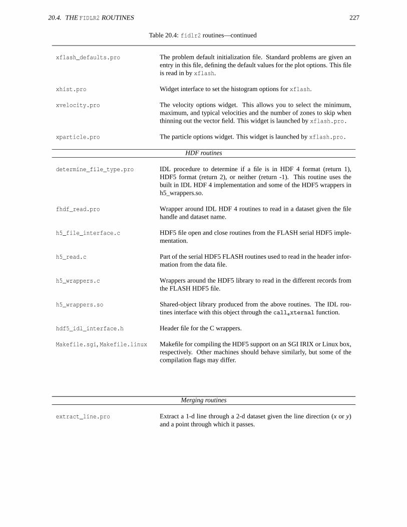
20.4. THE FIDLR2 ROUTINES 227
Table 20.4: fidlr2 routines—continued
xflash_defaults.pro The problem default initialization file. Standard problems are given anentry in this file, defining the default values for the plot options. This fileis read in by xflash.
xhist.pro Widget interface to set the histogram options for xflash.
xvelocity.pro The velocity options widget. This allows you to select the minimum,maximum, and typical velocities and the number of zones to skip whenthinning out the vector field. This widget is launched by xflash.pro.
xparticle.pro The particle options widget. This widget is launched by xflash.pro.
HDF routines
determine_file_type.pro IDL procedure to determine if a file is in HDF 4 format (return 1),HDF5 format (return 2), or neither (return -1). This routine uses thebuilt in IDL HDF 4 implementation and some of the HDF5 wrappers inh5_wrappers.so.
fhdf_read.pro Wrapper around IDL HDF 4 routines to read in a dataset given the filehandle and dataset name.
h5_file_interface.c HDF5 file open and close routines from the FLASH serial HDF5 imple-mentation.
h5_read.c Part of the serial HDF5 FLASH routines used to read in the header infor-mation from the data file.
h5_wrappers.c Wrappers around the HDF5 library to read in the different records fromthe FLASH HDF5 file.
h5_wrappers.so Shared-object library produced from the above routines. The IDL rou-tines interface with this object through the callexternal function.
hdf5_idl_interface.h Header file for the C wrappers.
Makefile.sgi, Makefile.linux Makefile for compiling the HDF5 support on an SGI IRIX or Linux box,respectively. Other machines should behave similarly, but some of thecompilation flags may differ.
Merging routines
extract_line.pro Extract a 1-d line through a 2-d dataset given the line direction (x or y)and a point through which it passes.
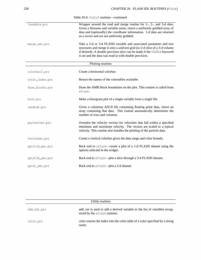
228 CHAPTER 20. FLASH IDL ROUTINES (FIDLR)
Table 20.4: fidlr2 routines—continued
loaddata.pro Wrapper around the read and merge routine for 1-, 2-, and 3-d data.Given a filename and variable name, return a uniformly gridded array ofdata and (optionally) the coordinate information. 1-d data are returnedas a vector and are not uniformly gridded.
merge_amr.pro Take a 2-d or 3-d FLASH variable and associated parameter and treestructures and merge it onto a uniform grid (or 2-d slice of a 3-d volumeif desired). A double precision slice can be made if the DOUBLE keywordis set and the data was read in with double precision.
Plotting routines
colorbar2.pro Create a horizontal colorbar.
color_index.pro Return the names of the colortables available.
draw_blocks.pro Draw the AMR block boundaries on the plot. This routine is called fromxflash.
hist.pro Make a histogram plot of a single variable from a single file.
readtab.pro Given a columnar ASCII file containing floating point data, return anarray containing that data. This routine automatically determines thenumber of rows and columns.
partvelvec.pro Overplot the velocity vectors for velocities that fall within a specifiedminimum and maximum velocity. The vectors are scaled to a typicalvelocity. This routine also handles the plotting of the particle data.
vcolorbar.pro Create a vertical colorbar given the data range and color bounds.
xplot1d_amr.pro Back end to xflash—create a plot of a 1-d FLASH dataset using theoptions selected in the widget.
xplot3d_amr.pro Back end to xflash—plot a slice through a 3-d FLASH dataset.
xplot_amr.pro Back end to xflash—plot a 2-d dataset.
Utility routines
add_var.pro add_var is used to add a derived variable to the list of variables recog-nized by the xflash routines.
color.pro color returns the index into the color table of a color specified by a stringname.
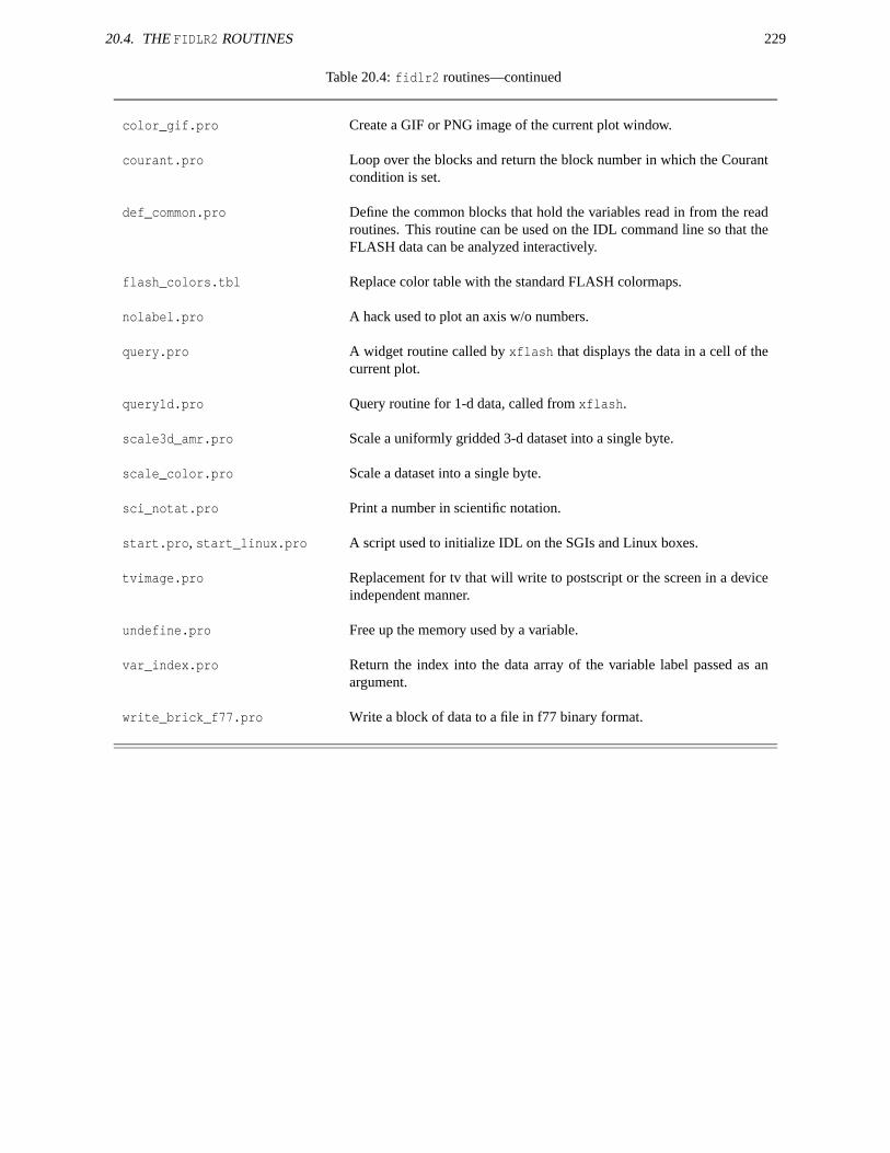
20.4. THE FIDLR2 ROUTINES 229
Table 20.4: fidlr2 routines—continued
color_gif.pro Create a GIF or PNG image of the current plot window.
courant.pro Loop over the blocks and return the block number in which the Courantcondition is set.
def_common.pro Define the common blocks that hold the variables read in from the readroutines. This routine can be used on the IDL command line so that theFLASH data can be analyzed interactively.
flash_colors.tbl Replace color table with the standard FLASH colormaps.
nolabel.pro A hack used to plot an axis w/o numbers.
query.pro A widget routine called by xflash that displays the data in a cell of thecurrent plot.
query1d.pro Query routine for 1-d data, called from xflash.
scale3d_amr.pro Scale a uniformly gridded 3-d dataset into a single byte.
scale_color.pro Scale a dataset into a single byte.
sci_notat.pro Print a number in scientific notation.
start.pro, start_linux.pro A script used to initialize IDL on the SGIs and Linux boxes.
tvimage.pro Replacement for tv that will write to postscript or the screen in a deviceindependent manner.
undefine.pro Free up the memory used by a variable.
var_index.pro Return the index into the data array of the variable label passed as anargument.
write_brick_f77.pro Write a block of data to a file in f77 binary format.
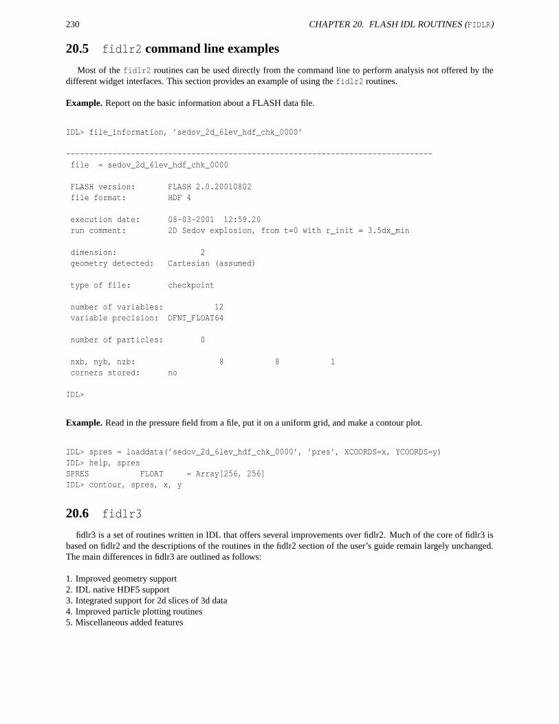
230 CHAPTER 20. FLASH IDL ROUTINES (FIDLR)
20.5 fidlr2 command line examples
Most of the fidlr2 routines can be used directly from the command line to perform analysis not offered by thedifferent widget interfaces. This section provides an example of using the fidlr2 routines.
Example. Report on the basic information about a FLASH data file.
IDL> file_information, ’sedov_2d_6lev_hdf_chk_0000’
-------------------------------------------------------------------------------file = sedov_2d_6lev_hdf_chk_0000
FLASH version: FLASH 2.0.20010802file format: HDF 4
execution date: 08-03-2001 12:59.20run comment: 2D Sedov explosion, from t=0 with r_init = 3.5dx_min
dimension: 2geometry detected: Cartesian (assumed)
type of file: checkpoint
number of variables: 12variable precision: DFNT_FLOAT64
number of particles: 0
nxb, nyb, nzb: 8 8 1corners stored: no
IDL>
Example. Read in the pressure field from a file, put it on a uniform grid, and make a contour plot.
IDL> spres = loaddata(’sedov_2d_6lev_hdf_chk_0000’, ’pres’, XCOORDS=x, YCOORDS=y)IDL> help, spresSPRES FLOAT = Array[256, 256]IDL> contour, spres, x, y
20.6 fidlr3
fidlr3 is a set of routines written in IDL that offers several improvements over fidlr2. Much of the core of fidlr3 isbased on fidlr2 and the descriptions of the routines in the fidlr2 section of the user’s guide remain largely unchanged.The main differences in fidlr3 are outlined as follows:
1. Improved geometry support2. IDL native HDF5 support3. Integrated support for 2d slices of 3d data4. Improved particle plotting routines5. Miscellaneous added features
20.6. FIDLR3 231
1. Improved geometry support
fidlr3 supports cartesian, cylindrical, polar and spherical geometries. The proper geometry should be detected byxflash using the geometry attribute in the HDF5 file header. Please note, however, that hdf5 versions 1.4.4-1.4.5-post2have a bug with Flash attributes in which all attribute names are mangled. If this is the case, xflash will prompt theuser for the proper geometry.
2. IDL native HDF5 support
In IDL versions 5.6 and above, native support of HDF5 has been added. This makes the building and use of theh5_wrapper.so library in fidlr2 obsolete. In practice, the following modifications must be made to the user’s environ-ment:
First, set the environment variable IDL_DIR to the root of your IDL installation:
setenv IDL_DIR /usr/local/rsi/idl_6.0
This can be done manually or through IDL setup scripts for your given shell which reside under $IDL_DIR/bin/idl_setup(for csh and related shells) and $IDL_DIR/bin/idl_setup.ksh (for bourne and related shells).
An XFLASH_DIR and IDL_PATH environment variable must be set manually:
setenv XFLASH_DIR <your_path_to_flash>/FLASH2.4/tools/fidlr3setenv IDL_PATH $IDL_DIR:$IDL_DIR/lib:$XFLASH_DIR
This is all that is required to enable IDL to read HDF5 data when using IDL 5.6 and above.
Caveat:
One problem with this approach is that as of IDL version 6.0, the native support for HDF5 cannot read data createdwith HDF5 versions 1.6.0 and above (currently 1.6.1 and 1.6.2). If you have data created with these versions of HDF5you must use fidlr2 and the h5_wrappers.
3. Integrated support for 2d slices of 3d data
fidlr3 can make 2d slices of 3d data. The routine used to do this is xplot3d_amr_new.pro, and is driven by xflash infidlr3. 3d data can be loaded within the GUI just as 2d data can. There are 3 toggle buttons marked “Slice Plane" forselecting x-y, x-z and y-z slices of 3d data.
4. Improved particle plotting routines
Newly present in FLASH2.4 checkpoint files is a dataset named “particle tracers", which can be accessed via the“Particle Options" button. The main particle plotting routine, “xparticle.pro", can then plot particle positions, particlevelocity vectors and the trajectory of a given particle across a set of checkpoint files. Please note that the dataset isnamed “particle tracers" for both active and passive particles in FLASH2.4.
Particle Positions and Velocity Vectors:
Once the particle options GUI has been brought up by pressing the “Particle Options" button there is first a togglefor enabling the plotting of particle positions. There one can also plot particle velocity vectors by pressing the “plotvelocity vectors" toggle button. To get meaningful velocity vectors it is necessary to have an idea of the range in
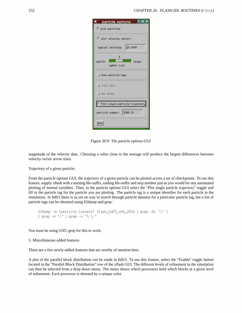
232 CHAPTER 20. FLASH IDL ROUTINES (FIDLR)
Figure 20.9: The particle options GUI
magnitude of the velocity data. Choosing a value close to the average will produce the largest differences betweenvelocity vector arrow sizes.
Trajectory of a given particle:
From the particle options GUI, the trajectory of a given particle can be plotted across a set of checkpoints. To use thisfeature, supply xflash with a starting file-suffix, ending file-suffix and step number just as you would for any automatedplotting of normal variables. Then, in the particle options GUI select the “Plot single particle trajectory" toggle andfill in the particle tag for the particle you are plotting. The particle tag is a unique identifier for each particle in thesimulation. In fidlr3 there is as yet no way to search through particle datasets for a particular particle tag, but a list ofparticle tags can be obtained using h5dump and grep:
h5dump -d "particle tracers" flash_hdf5_chk_0000 | grep -A1 "" \| grep -v "" | grep -v "\-\-"
You must be using GNU grep for this to work.
5. Miscellaneous added features
There are a few newly-added features that are worthy of mention here.
A plot of the parallel block distribution can be made in fidlr3. To use this feature, select the “Enable" toggle buttonlocated in the “Parallel Block Distribution" row of the xflash GUI. The different levels of refinement in the simulationcan then be selected from a drop down menu. The menu shows which processors hold which blocks at a given levelof refinement. Each processor is denoted by a unique color.

20.6. FIDLR3 233
From the IDL prompt, a “visual diff" can be made between any two variables in different files or the same file. Forexample, the command:
IDL> diff, ’<path_to_flash_hdf5_file>/flash_hdf5_0001’,’dens’, \’<path_to_flash_hdf5_file>/flash_hdf5_0002’,’dens’
would plot the difference between the ’dens’ variable in two different Flash hdf5 files.
Also present in the fidlr3 routines is the ability to read Flash data in netCDF format. Flash 2.4 will not contain anetCDF I/O module, but will in future releases.

234 CHAPTER 20. FLASH IDL ROUTINES (FIDLR)

Part V
Going Further with FLASH
235

Chapter 21
Adding new solvers
Adding new solvers (either for new or existing physics) to FLASH is similar in some ways to adding a problemconfiguration. In general, one creates a subdirectory for the solver, placing it under the source subdirectory for theparent module, if the solver implements currently supported physics, or creating a new module subdirectory, if it doesnot. Put the source files required by the solver into this directory and then create the following files:
Makefile: The make include file for the module should set a macro with the name of the module equal to a list of theobject files in the module. Optionally (recommended), add a list of dependencies for each of the source files in themodule. For example, the source_terms module’s make include file is
# Makefile for source term solvers
source_terms = source_termsModule.o burn.o heat.o cool.o init_burn.o init_heat.o \init_cool.o tstep_burn.o tstep_heat.o tstep_cool.o init_src.o
source_termsModule.o : source_termsModule.F90 dBase.oburn.o : burn.F90heat.o : heat.F90cool.o : cool.F90init_src.o : init_src.F90 dBase.oinit_burn.o : init_burn.F90init_heat.o : init_heat.F90init_cool.o : init_cool.F90tstep_burn.o : tstep_burn.F90tstep_heat.o : tstep_heat.F90tstep_cool.o : tstep_cool.F90
Sub-module make include files use macro concatenation to add to their parent modules’ make include files. Forexample, the source_terms/burn sub-module has the following make include file
237
238 CHAPTER 21. ADDING NEW SOLVERS
# Makefile for the nuclear burning sub-module
source_terms += burn_block.o net_auxillary.o net_integrate.o sparse_ma28.o \gift.o net.o shock_detect.o
burn_block.o : burn_block.F90 dBase.o network_common.fh eos_common.fh net.onet_auxillary.o : net_auxillary.F90 network_common.fh eos_common.fhnet_integrate.o : net_integrate.F90 network_common.fhsparse_ma28.o : sparse_ma28.F90net.o : net.F90 network_common.fh eos_common.fhgift.o : gift.F90shock_detect.o : shock_detect.F90 dBase.o
network_common.fh : network_size.fhtouch network_common.fh
# Additional dependencies
burn.o : dBase.o network_common.fh net.oinit_burn.o : dBase.o network_common.fh net.o
Note that the sub-module’s make include file only makes reference to files provided at its own level of the directoryhierarchy. If the sub-module provides special versions of routines to override those supplied by the parent module,they do not need to be mentioned again in the object list, because the sub-module’s Makefile is concatenated with itsparent’s. However, if these special versions have additional dependencies, they can be specified as shown. Of course,any files supplied by the sub-module that are not part of the parent module should be mentioned in the sub-module’sobject list, and their dependencies should be included.
If you are creating a new top-level module, your source files at this level will be included in the code, even if youdo not request the module in Modules. However, no sub-modules will be included. If you intend to have specialversions of these files (stubs) that are used when the module is not included, create a sub-module named null andplace them in it. null is automatically included if it is found and the module is not referenced in Modules.
If you create a top-level module with no Makefile, setup will automatically generate an empty one. For exam-ple, creating a directory named my_module/ in source/ causes setup to generate a Makefile.my_module in thebuild directory with contents
my_module =
If sub-modules of my_module exist and are requested, their Makefiles will be appended to this base.
Config: Create a configuration file for the module or sub-module you are creating. All configuration files in a sub-module path are used by setup, so a sub-module inherits its parent module’s configuration. Config should declare anyruntime parameters you wish to make available to the code when this module is included. It should indicate which (ifany) other modules your module requires in order to function, and it should indicate which (if any) of its sub-modulesshould be used as a default if none is specified when setup is run. The configuration file format is described in Sec. 4.1.
This is all that is necessary to add a module or sub-module to the code. However, it is not sufficient to have themodule routines called by the code! If you are creating a new solver for an existing physics module, the module itselfshould provide the interface layer to the rest of the code. As long as your sub-module provides the routines expectedby the interface layer, the sub-module should be ready to work. However, if you are adding a new module (or if yoursub-module has externally visible routines – a no-no for the future), you will need to add calls to your externally visibleroutines.
It is difficult to give complete general guidance; here we simply note a few things to keep in mind. If you wish tobe able to turn your module on or off without recompiling the code, create a new runtime parameter (e.g., use_module)
239
in the driver module. You can then test the value of this parameter before calling your externally visible routinesfrom the main code. For example, the burn module routines are only called if (iburn .eq. 1). (Of course, if theburn module is not included in the code, setting iburn to 1 will result in empty subroutine calls.)
You will need to add use dBase if you wish to have access to the global AMR data structure. Since this is theonly mechanism for operating on the grid data in FLASH, you will probably want to do this. An alternative, if yourmodule uses a pre-existing data structure, is to create an interface layer which converts the PARAMESH-inspired treedata structure used by FLASH into your data structure and then calls your routines. This will probably have someperformance impact, but it will enable you to get things working quickly.
You may wish to create an initialization routine for your module that is called before anything (e.g., setting initialconditions) is done. In this case you should call the routine init_module() and place a call to it (without any arguments)in the main initialization routine, init_flash.F90, which is part of the driver module. Be sure this routine has astub available.
If your solver introduces a constraint on the timestep, you should create a routine named tstep_module() thatcomputes this constraint. Add a call to this routine in timestep.F90 (part of the driver/time_dep module) usingyour global switch parameter, if you have created one. See this file for examples. Your routine should operate ona single block and take three parameters: the timestep variable (a real variable which you should set to the smallerof itself and your constraint before returning), the minimum timestep location (an integer array with five elements),and the block identifier (an integer). Returning anything for the minimum location is optional, but the other timesteproutines interpret it in the following way. The first three elements are set to the coordinates within the block of thezone contributing the minimum timestep. The fourth element is set to the block identifier, and the fifth is set to thecurrent processor identifier (MyPE). This information tags, along with the timestep constraint, when blocks and solversare compared across processors, and it is printed on stdout by the master processor along with the timestep informationas FLASH advances.
If your solver is time-dependent, you will need to add a call to your solver in the evolve() routine (driver/time_dep/evolve.F90).If it is time-independent, add the call to driver/steady/flash.F90. The default version of evolve() implementssecond-order Strang time splitting within the time loop maintained by driver/time_dep/flash.F90. The steadyversion of flash.F90 simply calls each operator once and then exits.
Try to limit the number of entry points to your module. This will make it easier to update it when the next versionof FLASH is released. It will also help to keep you sane.

240 CHAPTER 21. ADDING NEW SOLVERS
Chapter 22
Porting FLASH to other machines
Porting FLASH to new architectures should be fairly straightforward for most Unix or Unix-like systems. Forsystems which look nothing like Unix or which have no ability to interpret the setup script or makefiles, extensivereworking of the meta-code which configures and builds FLASH would be necessary. We do not treat such systemshere; rather than do so, it would be simpler for us to do the port ourselves. The good news in such cases is that,assuming that you can get the source tree configured on your system and that you have a Fortran 90 compiler and theother requirements discussed in Chapter 2, you should be able to compile the code without making too many changesto the source. We have generally tried to stick to standard Fortran 90, avoiding machine-specific features.
For Unix-like systems, you should make sure that your system has csh, a gmake that permits included makefiles,awk, sed, and python. Next, create a directory in source/sites/ with the name of your site (or a directory insource/sites/Prototypes/ with the name of your operating system). This directory should contain at least amakefile fragment named Makefile.h. The best way to start is to copy one of the existing makefile fragments toyour new directory and modify that. Makefile.h sets macros that define the names of your compilers, the compilerand linker flags, the names of additional object files needed for your machine but not included in the standard sourcedistribution, and additional shell commands (such as file renaming and deletion commands) needed for processing themaster makefile.
For most Unix systems, this will be all you need to do. However, in addition to Makefile.h you may need tocreate machine-specific subroutines that override the defaults included with the main source code. As long as thefiles containing these routines duplicate the existing routines’ filenames, they do not need to be added to the machine-dependent object list in Makefile.h; setup will automatically find the special routine in the system-specific directoryand link to it rather than to the general routine in the main source directories. An example of such a routine isgetarg(), which returns command-line arguments and is used by FLASH to read the name of the runtime parameterfile from the command line. This routine is not part of the Fortran 90 standard, but it is available on many Unixsystems without the need to link to a special library. However, it is not available on the Cray T3E; instead, a routinenamed pxfgetarg() provides the same functionality. Therefore, we have encapsulated the getarg() functionality ina routine named get_arguments(), which is part of the driver module, in a file named getarg.F90. The defaultversion simply calls getarg(). For the T3E, a replacement getarg.F90 that calls pxfgetarg() is supplied. Sincethis file overrides a default file with the same name, getarg.o does not need to be added to the machine-dependentobject list in source/sites/Prototypes/UNICOS/Makefile.h.
22.1 Writing a Makefile.h
To create a custom Makefile.h for your site, create a directory under source/sites that is the name returnedby hostname (e.g. sphere.uchicago.edu). In this directory, copy the Makefile.h from the Prototypes directory thatmatches your system most closely. Currently, the Makefile in sphere.uchicago.edu is usually the most up-to-date andshould be used as a starting point, if no other sites seem appropriate. To reflect your system, you must modify thedifferent macros defined in Makefile.
Listed and described below are macros defined in the Makefile.h:
FCOMP : the name of the Fortran 90 compiler
241
242 CHAPTER 22. PORTING FLASH TO OTHER MACHINES
CCOMP : the name of the C compiler
CPPCOMP : the name of the C++ compiler
LINK : the name of the linker (usually the Fortran compiler should serve as the linker)
PP : a flag (if any) that should precede a preprocessor directive (typically -D)
FFLAGS_OPT : the Fortran compilation flags to produce an optimized executable. These are theflags used when -auto is given to setup.
FFLAGS_DEBUG : the Fortran compilation flags to produce an executable that can be used with adebugger (e.g. totalview). These flags are used when -debug is passed to setup.
FFLAGS_TEST : Fortran compilation flags to produce an executable suitable for testing. Theseusually involve less optimization. These flags are used when -test is passed to setup.
CFLAGS_OPT : the optimized set of compilation flags for C/C++ code.
CFLAGS_DEBUG : the debug compilation flags for C/C++ code.
CFLAGS_TEST : the test compilation flags for C/C++ code.
LFLAGS_OPT : linker flags used with the _OPT compilation flags. This usually ends in ’-o’ torename the executable.
LFLAGS_DEBUG : linker flags used with the _DEBUG compilation.
LFLAGS_TEST : linker flags used with the _TEST compilation.
LIB_OPT : libraries to link in with the _OPT compilation. This should include the MPI libraryif an MPI wrapper for the linker was not used (e.g. mpif90).
LIB_DEBUG : libraries to link in the with the _DEBUG compilation.
LIB_TEST : libraries to link in with the _TEST compilation.
LIB_HDF4 : the necessary link line required to link the HDF4 library. This will be somethingof the form
L /path/to/library -lmfhdf -ldf -ljpeg -lz
LIB_HDF5 the necessary link line required to link in the HDF5 library. This will look somethinglike
-L /path/to/library -lhdf5
For example, here’s how you might modify the macros defined in the Makefile.h in sphere.uchicago.edu/.The first part of Makefile.h defines the paths for the libraries that FLASH requires (HDF/HDF5).
HDF4_PATH = /opt/pkgs/HDF/4.1r2_irix64v6.4-n32HDF5_PATH = /opt/pkgs/HDF5-1.4.0-irix64n32ZLIB_PATH = /opt/pkgs/zlib-1.1.3
These should be modified to reflect the locations on your system. For some machines, zlib isneeded in addition to the HDF5 library in order to resolve all of the dependencies.
22.1. WRITING A MAKEFILE.H 243
Next we setup the compilers and linker. We almost always use the Fortran 90 compiler as thelinker, so the Fortran libraries are automatically linked in.
FCOMP = f90CCOMP = ccCPPCOMP = CCLINK = f90
# pre-processor flagPP = -D
These commands will need to be changed if your compiler names are different. Note that on somesystems (i.e. those with MPICH as the MPI implementation), there are wrappers for the compilers(mpif90, mpicc, mpiCC) that automatically add the proper flags for the include files and the librariesto the link line when building. You are encouraged to use these wrappers. Some older versionsof MPICH do not recognize .F90 as a valid extension. For these, you can either update MPICH toa later version or edit mpif90 and add .F90 to the line that checks for a valid extension. ThePP macro refers to the pre-processor and should be set to the flag that the compiler uses to passinformation to the C preprocessor (usually -D).
We define three different setups of compiler flags as described earlier: the “_OPT” set fornormal, fully optimized code, the “_DEBUG” set for debugging FLASH, and the “_TEST” set for regressiontesting. This latter set usually has less optimization. These three sets are picked with the-auto, -debug, and -test flags to setup respectively.
FFLAGS_OPT = -c -Ofast=ip27 -OPT:Olimit=0:IEEE_arithmetic=3:roundoff=3 -IPA \-r8 -d8 -i4 -cpp -r10000 -LNO
FFLAGS_DEBUG = -c -DEBUG:subscript_check=ON:verbose_runtime=ON -r8 -d8 -i4 \-cpp -g
FFLAGS_TEST = -c -r8 -d8 -i4 -cpp -O2
F90FLAGS =
CFLAGS_OPT = -IPA -Ofast=ip27 -cCFLAGS_DEBUG = -g -cCFLAGS_TEST = -c -O2
Next come the linker flags. Typically, these have only -o to rename the executable, and somedebug flags (e.g. -g) for the “_DEBUG” set.
LFLAGS_OPT = -r8 -d8 -i4 -IPA -oLFLAGS_DEBUG = -r8 -d8 -i4 -g -oLFLAGS_TEST = -r8 -d8 -i4 -o
There are two different groups of library macros defined in the Makefile.h: one group correspondingto the “_OPT”, “_DEBUG”, “_TEST” flags defined above, and the other group for any libraries thatare required by a specific module (e.g. HDF5). Any module can require a certain library by puttinga line like
LIBRARY xxx
in its Config file. This library requirement will be satisfied in the Makefile.h by creatinga macro called LIB_xxx, and setting it equal to the libraries (including any path) that are requiredto resolve the dependencies in that module.
244 CHAPTER 22. PORTING FLASH TO OTHER MACHINES
For the sphere.uchicago.edu Makefile.h we have
LIB_HDF4 = -L$(HDF4_PATH)/lib -lmfhdf -ldf -lz
CFLAGS_HDF5 = -I $(HDF5_PATH)/includeLIB_HDF5 = -B static -L $(HDF5_PATH)/lib -lhdf5 \
-B dynamic -L $(ZLIB_PATH)/lib -lz
CFLAGS_VISTOOLS = -I /scratch2/caceres/python/include/python2.1LIB_VISTOOLS = -L /scratch2/caceres/python/src -lpython2.1 \
-lpthread
LIB_OPT = -L/usr/lib32 -lmpi -lfastmLIB_DEBUG = -L/usr/lib32 -lmpi -lfastmLIB_TEST = -L/usr/lib32 -lmpi
Note that there are also two CFLAGS_xxx macros here. They specify the include path for the libraryif any header files are needed. When setup generates the master Makefile, it will append theindividual CFLAGS_xxx lines to the master CFLAGS macro and the LIB_xxx lines to the master LIBmacro.
Finally, we have a macro to specify any platform dependent code and some macros for basic filemanipulation and library tools.
MACHOBJ =
MV = mv -fAR = ar -rRM = rm -fCD = cdRL = ranlibECHO = echo
On most platforms, these will not need to be modified.It is strongly suggested that you use the compiler flags from the prototype Makefile.h that
matches your system, if one exists. These are the flags that we use when testing FLASH.
Chapter 23
Troubleshooting
This section addresses some known problems that users and developers alike have encounteredin compiling and using FLASH on a number of different machines.
23.1 General questions about compiling FLASH
23.1.1 When I try to make FLASH, I get the following error:
make:file ‘Makefile.driver’ line 34: Must be a separator (: or ::) for rules (bu39)
FLASH requires the use of GNU make (usually called gmake) to build the code.
23.1.2 I noticed that FLASH uses the REAL declaration for single precision. Is there asimple way to make sure the computer calculates to DOUBLE PRECISION, eventhough the variables are defined with REAL?
Although the variables are all declared as real instead of double precision (or real*8) inthe code and constants are written as 1.e30 instead of 1.d30, the Makefiles for the differentplatforms use compiler switches to promote the reals to double precision. This is necessary,since on some platforms (e.g. Cray T3E), double precision is 16-byte precision.
23.1.3 When I make FLASH, lots of compilation lines are output, but no object (.o) files areproduced in object/—what’s up?
Older versions of MPICH do not recognize .F90 as a valid Fortran file extension in the mpif90compiler wrapper. All FLASH Fortran files end in .F90 to signify that they are free-form andrequire preprocessing. To fix this, edit the mpif90 wrapper and add ".F90" to the if test onthe file extension. It should look something like this
if [ "$ext" = ".f" -o "$ext" = ".F" -o "$ext" = ".f90" -o \"$ext" = ".for" -o "$ext" = ".FOR" -o "$ext" = ".F90" ] ; then
This should make mpif90 recognize .F90 files.
245
246 CHAPTER 23. TROUBLESHOOTING
23.2 Runtime errors
23.2.1 My problem hangs in refinement. Is there anything I can do?
This problem can be diagnosed by viewing the FLASH logfile. If your problem has hung, andthe last message of your logfile looks like this:
[ 08-17-2004 18:03.08 ] [AMR_REFINE_DEREFINE]: refinement initiated at 18:03.08
then chances are you’ve hung in refinement. This is a problem with the amr_redist_blk routine.There are three versions of the routine in the code: one chosen by default that’s faster butsometimes for unknown reasons hangs, and two others that are guaranteed not to hang. One of themis slower on most platforms and the newest one is slower on some platforms. To use one of them,resetup your problem including the additional module source/mesh/amr/paramesh2.0/amr_redist_blk_blockingor source/mesh/amr/paramesh2.0/amr_redist_blk_new..
We’ve observed this problem intermittently on the QSC system and possibly on intel linux systemswith the Portland Group fortran compiler version 5.1-3.
23.2.2 My problem ran fine, and I can look at data, but the HDF5 attributes are all blank.
This is a known problem when running FLASH with HDF5 versions 1.4.4 through 1.4.5-post2- HDF5attribute values are blank in FLASH checkpoints and plotfiles. HDF5 attributes in FLASH are usedto store descriptive information about the FLASH run, like which FLASH modules were included andthe geometry of the run, but actual grid data, like the values of variables, are stored as HDF5datasets which don’t have the same problem as the attributes. This error will allow running thecode and looking at most of the vital data in the FLASH run, but it’s not guaranteed that allfunctionality will work. To fix the problem, we recommend using FLASH with HDF5 version 1.4.3,or HDF5 version 1.6.2. Note that you need IDL version 6.1 or higher for the fidlr routines tobe compatible with HDF5 1.6.2 data format.
23.2.3 I ran a big problem, and in the performance summary, the number of zones persecond is negative.
Your run is fine- the problem is that the precision of the number that stores the value ofzones evolved is too small. The next version of FLASH or possibly a patch will fix this problem.
23.2.4 The detonation problem dies after the first timestep on an SGI with the error mes-sage:
matrix is structurally singular, rank = 1~.
Originally, the MIPS Pro 7.3.X series of compilers did not work properly with FLASH, and werecommended that users try dropping down to the 7.2 series, or else compile without the -IPA switch.However, skipping the interprocedural inlining will significantly affect performance. This problemhas been fixed by the 7.3.2.1m series compilers. A test suite comparison of the 7.2 series and7.3.2.1 compilers found no differences in the FLASH results.
23.2.5 I get an mmap error when running a large job (>∼ 32 processors) on an SGI.
Try recompiling and linking with the -64 switch (see the ABI man page). This will createa 64-bit executable. You will need to link in the 64-bit versions of the HDF libraries.
23.3. CONTACTING THE AUTHORS OF FLASH 247
23.2.6 FLASH runs for a while, but all of a sudden it stops, without printing any errors tostdout – what’s going on?
Most likely you’ve exceeded the maximum number of blocks that you have allocated on a processor- this is controlled by the MAXBLOCKS parameter. There may be an error message in the amr_logfile generated by the PARAMESH library. Possible errors include:
ERROR memory overflow in restrictNo. of blocks per processor exceeds maxblocks
There are two ways to fix this problem. Either increase the number of processors you are usingor increase the number of blocks per processor. To increase the number of blocks per processor,you need to rerun setup with the -maxblocks flag. For example, to setup the Sedov problem with1000 blocks per processor, use
./setup sedov -auto -maxblocks=1000
You want to ensure that the resulting executable fits into the available memory on a processor(leaving room for the operating system). You can check the size of the memory taken by the executablewith the size command. Since flash uses very little dynamically allocated memory, this is a goodmeasure of the memory requirements of FLASH. The default values of MAXBLOCKS are 500 for 2-d and200 for 3-d.
23.2.7 I can compile FLASH with HDF5 fine, but when I run, I get an error—“error whileloading shared libraries: libhdf5.so.0”. How do I get HDF5 output to work?
You’ve installed the shared-object library for HDF5 and linked to it fine, because you specifiedthe location of the library using -L on the link line. However, this library is not in your librarypath, so when the executable is run and tries to load it, it cannot find it. Try setting theLD_LIBRARY_PATH environment variable to the location of the library. For example, under tcsh
setenv LD_LIBRARY_PATH /opt/HDF5-1.x.x/lib
23.2.8 FLASH segmentation faults on an IBM when running on multiple processors, what’sup?
There is a bug in either FLASH (which we have not yet found) or in the AIX compilers thatprevents runtime_parameters.F90 from working on multiple processors when optimized with -O3 orhigher. If compiled with -O3, a segmentation fault will arise, because the pointer to the headof the integer linked list magically becomes null. The current work around is to compile with-O2.
23.2.9 When I run FLASH on an IBM machine using the AIX compilers, I get far moreblocks than I do on other platforms – how do I fix this?
Don’t use -qipa or -qhot with FLASH. It just doesn’t work. The issue is somewhere in thePARAMESH library, but it has not been worked out yet. If you are insistent, you can try compilingall of amr_*.F90 without -qipa/-qhot and the rest with these flags, but we’ve never tested FLASHin this manner and do not support it.
23.3 Contacting the authors of FLASH
FLASH is still under active development, so many desirable features have not yet been included.Also, you will most likely encounter bugs in the distributed code. A mailing list has been establishedfor reporting problems with the distributed FLASH code. To report a bug, send email to
248 CHAPTER 23. TROUBLESHOOTING
giving your name and contact information and a description of the procedure you were followingwhen you encountered the error. Information about the machine, operating system (uname -a), andcompiler you are using is also extremely helpful. Please do not send checkpoint files, as these can bevery large. If the problem can be reproduced with one of the standard test problems, send a copyof your runtime parameter file and your setup options. This situation is very desirable, as itlimits the amount of back-and-forth communication needed for us to reproduce the problem. Wecannot be responsible for problems that arise with a physics module or initial model you havedeveloped yourself, but we will generally try to help with these if you can narrow down the problemto an easily reproducible effect that occurs in a short program run and if you are willing tosupply your added source code.
We have also established a mailing list for FLASH users. This is a moderated mailing listand is intended both for FLASH users to communicate with each other about general usage issues(other than bugs) and for FLASH developers to announce the availability of new releases. Theaddress for this mailing list is
More information about FLASH can be obtained on the World Wide Web at
http://flash.uchicago.edu/
Chapter 24
References
Anninos, W. Y., & Norman, M. L. 1994, ApJ, 429, 434
Aparicio, J. M. 1998, ApJS, 117, 627
Bader, G. & Deuflhard, P. 1983, NuMat, 41, 373
Bardeen, J. M., Bond, J. R., Kaiser, N., & Szalay, A. S. 1986, ApJ, 304, 15
Berger, M. J. & Collela, P. 1989, JCP, 82, 64
Berger, M. J. & Oliger, J. 1984, JCP, 53, 484
Blinnikov, S. I., Dunina-Barkovskaya, N. V., & Nadyozhin, D. K. 1996, ApJS, 106, 171
Boris, J. P. & Book, D. L. 1973, JCP, 11, 38
Brackbill, J. & Barnes, D. C. 1980 JCP, 35, 426
Brandt, A. 1977, Math. Comp., 31, 333
Brio, M. & Wu, C. C. 1988 JCP, 75, 400
Brown, P. N., Byrne, G. D., & Hindmarsh, A. C. 1989, SIAM J. Sci. Stat. Comput., 10, 1038
Bunn, E. F. & White, M. 1997, ApJ, 480, 6
Burgers, J. M. 1969, Flow Equations for Composite Gases (New York: Academic)
Caughlan, G. R. & Fowler, W. A. 1988, Atomic Data and Nuclear Data Tables, 40, 283
Chandrasekhar, S. 1961, Hydrodynamic and Hydromagnetic Stability (Oxford: Clarendon)
Chandrasekhar, S. 1939, An Introduction to the Study of Stellar Structure (Toronto: Dover)
Chandrasekhar, S. 1987, Ellipsoidal Figures of Equilibrium (New York: Dover)
Chapman, S. & Cowling, T. G. 1970, The Mathematical Theory of Non-uniform Gases (Cambridge: CUP)
Christy, R. F. 1966, ApJ, 144, 108
Colella, P. & Glaz, H. M. 1985, JCP, 59, 264
Colella, P. & Woodward, P. 1984, JCP, 54, 174
Colgate, S. A., & White, R. H. 1966, ApJ, 143, 626
Decyk, V. K., Norton, C. D., & Szymanski, B. K. 1997, ACM Fortran Forum, 16 (alsohttp://www.cs.rpi.edu/~szymansk/oof90.html)
249
250 CHAPTER 24. REFERENCES
DeZeeuw, D. & Powell, K. G. 1993, JCP, 104, 56
Duff, I. S., Erisman, A. M., & Reid, J. K. 1986, Direct Methods for Sparse Matrices (Oxford:Clarendon Press)
Emery, A. F. 1968, JCP, 2, 306
Eswaran, V. and Pope, S. B. 1988, Computers & Fluids, 16, 257-278
Evans, C. R. & Hawley, J. F. 1988, ApJ, 332, 659
Fletcher, C. A. J. 1991, Computational Techniques for Fluid Dynamics, 2d ed. (Berlin: Springer-Verlag)
Forester, C. K. 1977, JCP, 23, 1
Foster, P. N., & Chevalier, R. A. 1993, ApJ, 416, 303
Fryxell, B. A., Müller, E., & Arnett, D. 1989, in Numerical Methods in Astrophysics, ed. P. R. Woodward(New York: Academic)
Fryxell, B., Olson, K., Ricker, P., Timmes, F. X., Zingale, M., Lamb, D. Q., MacNeice, P., Rosner,R., Truran, J. W., & Tufo, H. 2000, ApJS, 131, 273
Godunov, S. K. 1959, Mat. Sbornik, 47, 271
Hu, W. & Sugiyama, N. 1996, ApJ, 471, 542
Huang, J., & Greengard, L. 2000, SIAM. J. Sci. Comput., 21, 1551
Iben, I. Jr. 1975, ApJ, 196, 525
Itoh, N., Hayashi, H., Nishikawa, A., & Kohyama, Y. 1996, ApJS, 102, 411
James, R. A. 1977, JCP, 25, 71
Jeans, J. H. 1902, Phil. Trans. Roy. Soc. (London), 199, 1
Khokhlov, A. M. 1997, Naval Research Lab memo 6406-97-7950
Kurganov, A., Noelle, S., & Petrova, G. 2001, SIAM. J. 23, 707
Kurganov, A., & Tadmor, E. 2000 JCP, 160, 241
Lacey, C. G. & Cole, S. 1993, MNRAS, 262, 627
Löhner, R. 1987, Comp. Meth. App. Mech. Eng., 61, 323
LeVeque, R. J. 1997, JCP, 131, 327
LeVeque, R. J. 1998, “Nonlinear Convservation Laws and Finite Volume Methods”, R. J. LeVeque,D. Mihalas, E. A. Dorfi, E. Mueller (ed.), Computational Methods for Astrophysical FluidFlow, Springer.
Linde, T., & Malagoli, A. 2001, JCP, submitted
MacNeice, P., Olson, K. M., Mobarry, C., de Fainchtein, R., & Packer, C. 1999, CPC, accepted
Marder, B. 1987, JCP, 68, 48
Martin, D., & Cartwright, K. 1996, “Solving Poisson’s Equation using Adaptive Mesh Refinement.”(http://seesar.lbl.gov/anag/staff/martin/AMRPoisson.html)
Mönchmeyer, R., & Müller, E. 1989, A&A, 217, 351
251
Munz, C. D., Omnes, P., Schneider, R., Sonnendrücker, & Voß, U. 2000, JCP, 161, 484
Nadyozhin, D. K. 1974, Nauchnye informatsii Astron, Sov. USSR, 32, 33
Orszag, S. A., Tang, C.-M., 1979, JFM, 90, 129
Parashar M., 1999, private communication (http://www.caip.rutgers.edu/~parashar/DAGH)
Plewa, T. & Müller, E. 1999, A&A, 342, 179.
Potekhin, A. Y., Chabrier, G., & Yakovlev, D. G. 1997, A&A323, 415
Powell, K. G., Roe, P. L., Linde, T. J. , Gombosi, T. I., & DeZeeuw, D. L. 1999, JCP, 154, 284
Press, W. H., Teukolsky, S. A., Vetterling, W. T., & Flannery, B. P. 1992, Numerical Recipesin Fortran, 2d ed. (Cambridge: CUP)
Quirk, J. J., in Upwind and High-Resolution Schemes, ed. M. Yousuff Hussaini, Bram van Leer,and John Van Rosendale, 1997, (Berlin: Springer).
Ross, R., Nurmi, D., Cheng, A. & Zingale, M. 2001, Proceedings of SC2001.
Sedov, L. I. 1959, Similarity and Dimensional Methods in Mechanics (New York: Academic)
Shu, C.-W. 1998, in Advanced Numerical Approximation of Nonlinear Hyperbolic Equations, ed. A. Quarteroni,Lecture Notes in Mathematics, 1697, (Springer: Berlin)
Shu, C.-W. & Osher, S. 1989, JCP, 83, 32
Spitzer, L. 1962, Physics of Fully Ionized Gases. (New York: Wiley)
Sportisse, B. 2000, JCP, 161, 140
Sod, G. 1978, JCP, 27, 1
Strang, G. 1968, SIAM J. Numer. Anal., 5, 506
Timmes, F. X. 1992, ApJ, 390, L107
Timmes, F. X. 1999, ApJS, 124, 241
Timmes, F. X. 2000, ApJ, 528, 913
Timmes, F. X. & Arnett, D. 2000, ApJS, 125, 294
Timmes, F. X. & Brown, E. 2002 (in preparation)
Timmes, F. X. & Swesty, F. D. 2000, ApJS, 126, 501
Toro, E. F. 1997, Riemann Solvers and Numerical Methods for Fluid Dynamics. (New York: Springer-Verlag)
Tóth, G. 2000, JCP, 161, 605
Trottenberg, U., Oosterlee, C., & Schüller, A. 2001, Multigrid (San Diego: Academic Press)
van Leer, B. 1979, JCP, 32, 101
Wallace, R. K., Woosley, S. E., & Weaver, T. A. 1982, ApJ, 258, 696
Warren, M. S. & Salmon, J. K. 1993, in Proc. Supercomputing 1993 (Washington, DC: IEEE ComputerSoc.)
Weaver, T. A., Zimmerman, G. B., & Woosley, S. E. 1978, ApJ, 225, 1021
Williams, F. A. 1988, Combustion Theory (Menlo Park: Benjamin-Cummings)
252 CHAPTER 24. REFERENCES
Williamson, J. H. 1980, JCP, 35, 48
Woodward, P. & Colella, P. 1984, JCP, 54, 115
Yakovlev, D. G., & Urpin, V. A. (YU) 1980 24, 303
Yee, H. C., Vinokur, M., and Djomehri, M. J. 2000, JCP, 162, 33
Zalesak, S. T. 1987, in Advances in Computer Methods for Partial Differential Equations VI, eds. Vichnevetsky,R. and Stepleman, R. S. (IMACS), 15
Zel’dovich, Ya. B. 1970, A&A, 5, 84
Zingale, M., Dursi, L. J., ZuHone, J., Calder, A. C., Fryxell, B., Plewa, T., Truran, J. W., Caceres,A., Olson, K., Ricker, P. M., Riley, K., Rosner, R., Siegel, A., Timmes, F. X., and Vladimirova,N. 2002, ApJS, 143, 539