Flat systems, equivalence and trajectory

generation

Ph. Martin∗ R. M. Murray† P. Rouchon∗

Technical report, April 2003

Abstract

Flat systems, an important subclass of nonlinear control systems in-troduced via differential-algebraic methods, are defined in a differentialgeometric framework. We utilize the infinite dimensional geometry devel-oped by Vinogradov and coworkers: a control system is a diffiety, or moreprecisely, an ordinary diffiety, i.e. a smooth infinite-dimensional manifoldequipped with a privileged vector field. After recalling the definition ofa Lie-Backlund mapping, we say that two systems are equivalent if theyare related by a Lie-Backlund isomorphism. Flat systems are those sys-tems which are equivalent to a controllable linear one. The interest ofsuch an abstract setting relies mainly on the fact that the above systemequivalence is interpreted in terms of endogenous dynamic feedback. Thepresentation is as elementary as possible and illustrated by the VTOLaircraft.

1 Introduction

Control systems are ubiquitous in modern technology. The use of feedback con-trol can be found in systems ranging from simple thermostats that regulate thetemperature of a room, to digital engine controllers that govern the operation ofengines in cars, ships, and planes, to flight control systems for high performanceaircraft. The rapid advances in sensing, computation, and actuation technolo-gies is continuing to drive this trend and the role of control theory in advanced(and even not so advanced) systems is increasing.

A typical use of control theory in many modern systems is to invert thesystem dynamics to compute the inputs required to perform a specific task.This inversion may involve finding appropriate inputs to steer a control systemfrom one state to another or may involve finding inputs to follow a desired

∗Centre Automatique et Systemes, Ecole des Mines de Paris, 35 rue Saint-Honore, 77305Fontainebleau, FRANCE. [martin,rouchon]@cas.ensmp.fr.

†Division of Engineering and Applied Science, California Institute of Technology, Pasadena,CA 91125, USA. murray@cds.caltech.edu.

1

trajectory for some or all of the state variables of the system. In general, thesolution to a given control problem will not be unique, if it exists at all, and soone must trade off the performance of the system for the stability and actuationeffort. Often this tradeoff is described as a cost function balancing the desiredperformance objectives with stability and effort, resulting in an optimal controlproblem.

This inverse dynamics problem assumes that the dynamics for the systemare known and fixed. In practice, uncertainty and noise are always present insystems and must be accounted for in order to achieve acceptable performanceof this system. Feedback control formulations allow the system to respondto errors and changing operating conditions in real-time and can substantiallyaffect the operability of the system by stabilizing the system and extending itscapabilities. Again, one may formulate the feedback regulation problems asan optimization problem to allow tradeoffs between stability, performance, andactuator effort.

The basic paradigm used in most, if not all, control techniques is to exploitthe mathematical structure of the system to obtain solutions to the inversedynamics and feedback regulation problems. The most common structure toexploit is linear structure, where one approximates the given system by its lin-earization and then uses properties of linear control systems combined with ap-propriate cost function to give closed form (or at least numerically computable)solutions. By using different linearizations around different operating points, itis even possible to obtain good results when the system is nonlinear by “schedul-ing” the gains depending on the operating point.

As the systems that we seek to control become more complex, the use oflinear structure alone is often not sufficient to solve the control problems that arearising in applications. This is especially true of the inverse dynamics problems,where the desired task may span multiple operating regions and hence the useof a single linear system is inappropriate.

In order to solve these harder problems, control theorists look for differenttypes of structure to exploit in addition to simple linear structure. In thispaper we concentrate on a specific class of systems, called “(differentially) flatsystems”, for which the structure of the trajectories of the (nonlinear) dynamicscan be completely characterized. Flat systems are a generalization of linearsystems (in the sense that all linear, controllable systems are flat), but thetechniques used for controlling flat systems are much different than many of theexisting techniques for linear systems. As we shall see, flatness is particularlywell tuned for allowing one to solve the inverse dynamics problems and onebuilds off of that fundamental solution in using the structure of flatness to solvemore general control problems.

Flatness was first defined by Fliess et al. [19, 22] using the formalism ofdifferential algebra, see also [53] for a somewhat different approach. In differ-ential algebra, a system is viewed as a differential field generated by a set ofvariables (states and inputs). The system is said to be flat if one can find a setof variables, called the flat outputs, such that the system is (non-differentially)algebraic over the differential field generated by the set of flat outputs. Roughly

2

speaking, a system is flat if we can find a set of outputs (equal in number to thenumber of inputs) such that all states and inputs can be determined from theseoutputs without integration. More precisely, if the system has states x ∈ Rn,and inputs u ∈ Rm then the system is flat if we can find outputs y ∈ Rm of theform

y = h(x, u, u, . . . , u(r))

such that

x = ϕ(y, y, . . . , y(q))

u = α(y, y, . . . , y(q)).

More recently, flatness has been defined in a more geometric context, wheretools for nonlinear control are more commonly available. One approach is to useexterior differential systems and regard a nonlinear control system as a Pfaffiansystem on an appropriate space [110]. In this context, flatness can be describedin terms of the notion of absolute equivalence defined by E. Cartan [8, 9, 104].

In this paper we adopt a somewhat different geometric point of view, relyingon a Lie-Backlund framework as the underlying mathematical structure. Thispoint of view was originally described in [20, 23, 24] and is related to the workof Pomet et al. [87, 85] on “infinitesimal Brunovsky forms” (in the context offeedback linearization). It offers a compact framework in which to describebasic results and is also closely related to the basic techniques that are usedto compute the functions that are required to characterize the solutions of flatsystems (the so-called flat outputs).

Applications of flatness to problems of engineering interest have grown steadilyin recent years. It is important to point out that many classes of systems com-monly used in nonlinear control theory are flat. As already noted, all con-trollable linear systems can be shown to be flat. Indeed, any system that canbe transformed into a linear system by changes of coordinates, static feedbacktransformations (change of coordinates plus nonlinear change of inputs), or dy-namic feedback transformations is also flat. Nonlinear control systems in “purefeedback form”, which have gained popularity due to the applicability of back-stepping [41] to such systems, are also flat. Thus, many of the systems forwhich strong nonlinear control techniques are available are in fact flat systems,leading one to question how the structure of flatness plays a role in control ofsuch systems.

One common misconception is that flatness amounts to dynamic feedbacklinearization. It is true that any flat system can be feedback linearized usingdynamic feedback (up to some regularity conditions that are generically satis-fied). However, flatness is a property of a system and does not imply that oneintends to then transform the system, via a dynamic feedback and appropriatechanges of coordinates, to a single linear system. Indeed, the power of flatnessis precisely that it does not convert nonlinear systems into linear ones. Whena system is flat it is an indication that the nonlinear structure of the system iswell characterized and one can exploit that structure in designing control algo-rithms for motion planning, trajectory generation, and stabilization. Dynamic

3

feedback linearization is one such technique, although it is often a poor choiceif the dynamics of the system are substantially different in different operatingregimes.

Another advantage of studying flatness over dynamic feedback linearizationis that flatness is a geometric property of a system, independent of coordinatechoice. Typically when one speaks of linear systems in a state space context,this does not make sense geometrically since the system is linear only in certainchoices of coordinate representations. In particular, it is difficult to discuss thenotion of a linear state space system on a manifold since the very definitionof linearity requires an underlying linear space. In this way, flatness can beconsidered the proper geometric notion of linearity, even though the systemmay be quite nonlinear in almost any natural representation.

Finally, the notion of flatness can be extended to distributed parameterssystems with boundary control and is useful even for controlling linear systems,whereas feedback linearization is yet to be defined in that context.

2 Equivalence and flatness

2.1 Control systems as infinite dimensional vector fields

A system of differential equations

x = f(x), x ∈ X ⊂ Rn (1)

is by definition a pair (X, f), where X is an open set of Rn and f is a smoothvector field on X . A solution, or trajectory, of (1) is a mapping t → x(t) suchthat

x(t) = f(x(t)) ∀t ≥ 0.

Notice that if x → h(x) is a smooth function on X and t → x(t) is a trajectoryof (1), then

d

dth(x(t)) =

∂h

∂x(x(t)) · x(t) =

∂h

∂x(x(t)) · f(x(t)) ∀t ≥ 0.

For that reason the total derivative, i.e., the mapping

x → ∂h

∂x(x) · f(x)

is somewhat abusively called the “time-derivative” of h and denoted by h.We would like to have a similar description, i.e., a “space” and a vector field

on this space, for a control system

x = f(x, u), (2)

where f is smooth on an open subset X ×U ⊂ Rn ×R

m. Here f is no longer avector field on X , but rather an infinite collection of vector fields on X param-eterized by u: for all u ∈ U , the mapping

x → fu(x) = f(x, u)

4

is a vector field on X . Such a description is not well-adapted when consideringdynamic feedback.

It is nevertheless possible to associate to (2) a vector field with the “same”solutions using the following remarks: given a smooth solution of (2), i.e., amapping t → (x(t), u(t)) with values in X × U such that

x(t) = f(x(t), u(t)) ∀t ≥ 0,

we can consider the infinite mapping

t → ξ(t) = (x(t), u(t), u(t), . . .)

taking values in X ×U ×R∞m , where R∞

m = Rm ×Rm × . . . denotes the productof an infinite (countable) number of copies of Rm. A typical point of R∞

m is thusof the form (u1, u2, . . .) with ui ∈ Rm. This mapping satisfies

ξ(t) =(f(x(t), u(t)), u(t), u(t), . . .

) ∀t ≥ 0,

hence it can be thought of as a trajectory of the infinite vector field

(x, u, u1, . . .) → F (x, u, u1, . . .) = (f(x, u), u1, u2, . . .)

on X × U × R∞m . Conversely, any mapping

t → ξ(t) = (x(t), u(t), u1(t), . . .)

that is a trajectory of this infinite vector field necessarily takes the form (x(t), u(t), u(t), . . .)with x(t) = f(x(t), u(t)), hence corresponds to a solution of (2). Thus F is trulya vector field and no longer a parameterized family of vector fields.

Using this construction, the control system (2) can be seen as the data of the“space” X × U × R∞

m together with the “smooth” vector field F on this space.Notice that, as in the uncontrolled case, we can define the “time-derivative”of a smooth function (x, u, u1, . . .) → h(x, u, u1, . . . , uk) depending on a finitenumber of variables by

h(x, u, u1, . . . , uk+1) := Dh · F=∂h

∂x· f(x, u) +

∂h

∂u· u1 +

∂h

∂u1· u2 + · · · .

The above sum is finite because h depends on finitely many variables.

Remark 1. To be rigorous we must say something of the underlying topologyand differentiable structure of R∞

m to be able to speak of smooth objects [113].This topology is the Frechet topology, which makes things look as if we wereworking on the product of k copies of Rm for a “large enough” k. For ourpurpose it is enough to know that a basis of the open sets of this topology consistsof infinite products U0×U1×. . . of open sets of Rm, and that a function is smoothif it depends on a finite but arbitrary number of variables and is smooth in the

5

usual sense. In the same way a mapping Φ : R∞m → R∞

n is smooth if all of itscomponents are smooth functions.

R∞m equipped with the Frechet topology has very weak properties: useful the-

orems such as the implicit function theorem, the Frobenius theorem, and thestraightening out theorem no longer hold true. This is only because R

∞m is a

very big space: indeed the Frechet topology on the product of k copies of Rm forany finite k coincides with the usual Euclidian topology.

We can also define manifolds modeled on R∞m using the standard machinery.

The reader not interested in these technicalities can safely ignore the details andwon’t loose much by replacing “manifold modeled on R∞

m” by “open set of R∞m”.

We are now in position to give a formal definition of a system:

Definition 1. A system is a pair (M, F ) where M is a smooth manifold, possiblyof infinite dimension, and F is a smooth vector field on M.

Locally, a control system looks like an open subset of Rα (α not necessarilyfinite) with coordinates (ξ1, . . . , ξα) together with the vector field

ξ → F (ξ) = (F1(ξ), . . . , Fα(ξ))

where all the components Fi depend only on a finite number of coordinates. Atrajectory of the system is a mapping t → ξ(t) such that ξ(t) = F (ξ(t)).

We saw in the beginning of this section how a “traditional” control systemfits into our definition. There is nevertheless an important difference: we losethe notion of state dimension. Indeed

x = f(x, u), (x, u) ∈ X × U ⊂ Rn × R

m (3)

andx = f(x, u), u = v (4)

now have the same description (X × U × R∞m , F ), with

F (x, u, u1, . . .) = (f(x, u), u1, u2, . . .),

in our formalism: t → (x(t), u(t)) is a trajectory of (3) if and only if t →(x(t), u(t), u(t)) is a trajectory of (4). This situation is not surprising since thestate dimension is of course not preserved by dynamic feedback. On the otherhand we will see there is still a notion of input dimension.

Example 1 (The trivial system). The trivial system (R∞m , Fm), with coor-

dinates (y, y1, y2, . . .) and vector field

Fm(y, y1, y2, . . .) = (y1, y2, y3, . . .)

describes any “traditional” system made of m chains of integrators of arbitrarylengths, and in particular the direct transfer y = u.

6

In practice we often identify the “system” F (x, u) := (f(x, u), u1, u2, . . .)with the “dynamics” x = f(x, u) which defines it. Our main motivation forintroducing a new formalism is that it will turn out to be a natural frameworkfor the notions of equivalence and flatness we want to define.

Remark 2. It is easy to see that the manifold M is finite-dimensional onlywhen there is no input, i.e., to describe a determined system of differentialequations one needs as many equations as variables. In the presence of inputs,the system becomes underdetermined, there are more variables than equations,which accounts for the infinite dimension.

Remark 3. Our definition of a system is adapted from the notion of diffietyintroduced in [113] to deal with systems of (partial) differential equations. Bydefinition a diffiety is a pair (M, CTM) where M is smooth manifold, possiblyof infinite dimension, and CTM is an involutive finite-dimensional distributionon M, i.e., the Lie bracket of any two vector fields of CTM is itself in CTM.The dimension of CTM is equal to the number of independent variables.

As we are only working with systems with lumped parameters, hence governedby ordinary differential equations, we consider diffieties with one dimensionaldistributions. For our purpose we have also chosen to single out a particularvector field rather than work with the distribution it spans.

2.2 Equivalence of systems

In this section we define an equivalence relation formalizing the idea that twosystems are “equivalent” if there is an invertible transformation exchangingtheir trajectories. As we will see later, the relevance of this rather naturalequivalence notion lies in the fact that it admits an interpretation in terms ofdynamic feedback.

Consider two systems (M, F ) and (N, G) and a smooth mapping Ψ : M → N(remember that by definition every component of a smooth mapping dependsonly on finitely many coordinates). If t → ξ(t) is a trajectory of (M, F ), i.e.,

∀ξ, ξ(t) = F (ξ(t)),

the composed mapping t → ζ(t) = Ψ(ξ(t)) satisfies the chain rule

ζ(t) =∂Ψ∂ξ

(ξ(t)) · ξ(t) =∂Ψ∂ξ

(ξ(t)) · F (ξ(t)).

The above expressions involve only finite sums even if the matrices and vectorshave infinite sizes: indeed a row of ∂Ψ

∂ξ contains only a finite number of non zeroterms because a component of Ψ depends only on finitely many coordinates.Now, if the vector fields F and G are Ψ-related, i.e.,

∀ξ, G(Ψ(ξ)) =∂Ψ∂ξ

(ξ) · F (ξ)

7

thenζ(t) = G(Ψ(ξ(t)) = G(ζ(t)),

which means that t → ζ(t) = Ψ(ξ(t)) is a trajectory of (N, G). If moreover Ψhas a smooth inverse Φ then obviously F,G are also Φ-related, and there is aone-to-one correspondence between the trajectories of the two systems. We callsuch an invertible Ψ relating F and G an endogenous transformation.

Definition 2. Two systems (M, F ) and (N, G) are equivalent at (p, q) ∈ M×Nif there exists an endogenous transformation from a neighborhood of p to aneighborhood of q. (M, F ) and (N, G) are equivalent if they are equivalent atevery pair of points (p, q) of a dense open subset of M × N.

Notice that when M and N have the same finite dimension, the systems arenecessarily equivalent by the straightening out theorem. This is no longer truein infinite dimensions.

Consider the two systems (X×U ×R∞m , F ) and (Y ×V ×R

∞s , G) describing

the dynamics

x = f(x, u), (x, u) ∈ X × U ⊂ Rn × R

m (5)y = g(y, v), (y, v) ∈ Y × V ⊂ R

r × Rs. (6)

The vector fields F,G are defined by

F (x, u, u1, . . .) = (f(x, u), u1, u2, . . .)

G(y, v, v1, . . .) = (g(y, v), v1, v2, . . .).

If the systems are equivalent, the endogenous transformation Ψ takes the form

Ψ(x, u, u1, . . .) = (ψ(x, u), β(x, u), β(x, u), . . .).

Here we have used the short-hand notation u = (u, u1, . . . , uk), where k is somefinite but otherwise arbitrary integer. Hence Ψ is completely specified by themappings ψ and β, i.e, by the expression of y, v in terms of x, u. Similarly, theinverse Φ of Ψ takes the form

Φ(y, v, v1, . . .) = (ϕ(y, v), α(y, v), α(y, v), . . .).

As Ψ and Φ are inverse mappings we have

ψ(ϕ(y, v), α(y, v)

)= y

β(ϕ(y, v), α(y, v)

)= v

andϕ(ψ(x, u), β(x, u)

)= x

α(ψ(x, u), β(x, u)

)= u.

Moreover F and G Ψ-related implies

f(ϕ(y, v), α(y, v)

)= Dϕ(y, v) · g(y, v)

where g stands for (g, v1, . . . , vk), i.e., a truncation of G for some large enough k.Conversely,

g(ψ(x, u), β(y, u)

)= Dψ(x, u) · f(y, u).

8

In other words, whenever t → (x(t), u(t)) is a trajectory of (5)

t → (y(t), v(t)) =(ϕ(x(t), u(t)), α(x(t), u(t))

)is a trajectory of (6), and vice versa.

Example 2 (The PVTOL). The system generated by

x = −u1 sin θ + εu2 cos θz = u1 cos θ + εu2 sin θ − 1

θ = u2.

is globally equivalent to the systems generated by

y1 = −ξ sin θ, y2 = ξ cos θ − 1,

where ξ and θ are the control inputs. Indeed, setting

X := (x, z, x, z, θ, θ)U := (u1, u2)

andY := (y1, y2, y1, y2)V := (ξ, θ)

and using the notations in the discussion after definition 2, we define the map-pings Y = ψ(X,U) and V = β(X,U) by

ψ(X,U) :=

x− ε sin θz + ε cos θx− εθ cos θz − εθ sin θ

and β(X,U) :=

(u1 − εθ2

θ

)

to generate the mapping Ψ. The inverse mapping Φ is generated by the mappingsX = ϕ(Y, V ) and U = α(Y, V ) defined by

ϕ(Y, V ) :=

y1 + ε sin θy2 − ε cos θy1 + εθ cos θy2 − εθ sin θ

θ

θ

and α(Y, V ) :=(ξ + εθ2

θ

)

An important property of endogenous transformations is that they preservethe input dimension:

Theorem 1. If two systems (X×U×R∞m , F ) and (Y×V×R∞

s , G) are equivalent,then they have the same number of inputs, i.e., m = s.

Proof. Consider the truncation Φµ of Φ on X × U × (Rm)µ,

Φµ : X × U × (Rm+k)µ → Y × V × (Rs)µ

(x, u, u1, . . . , uk+µ) → (ϕ, α, α, . . . , α(µ)),

9

i.e., the first µ + 2 blocks of components of Ψ; k is just a fixed “large enough”integer. Because Ψ is invertible, Ψµ is a submersion for all µ. Hence thedimension of the domain is greater than or equal to the dimension of the range,

n+m(k + µ+ 1) ≥ s(µ+ 1) ∀µ > 0,

which implies m ≥ s. Using the same idea with Ψ leads to s ≥ m.

Remark 4. Our definition of equivalence is adapted from the notion of equiva-lence between diffieties. Given two diffieties (M, CTM) and (N, CTN), we saythat a smooth mapping Ψ from (an open subset of) M to N is Lie-Backlundif its tangent mapping TΨ satisfies TΦ(CTM) ⊂ CTN. If moreover Ψ has asmooth inverse Φ such that TΨ(CTN) ⊂ CTM, we say it is a Lie-Backlundisomorphism. When such an isomorphism exists, the diffieties are said to beequivalent. An endogenous transformation is just a special Lie-Backlund iso-morphism, which preserves the time parameterization of the integral curves. Itis possible to define the more general concept of orbital equivalence [20, 18] byconsidering general Lie-Backlund isomorphisms, which preserve only the geo-metric locus of the integral curves.

2.3 Differential Flatness

We single out a very important class of systems, namely systems equivalent toa trivial system (R∞

s , Fs) (see example 1):

Definition 3. The system (M, F ) is flat at p ∈ M (resp. flat) if it equivalentat p (resp. equivalent) to a trivial system.

We specialize the discussion after definition 2 to a flat system (X×U×R∞m , F )

describing the dynamics

x = f(x, u), (x, u) ∈ X × U ⊂ Rn × R

m.

By definition the system is equivalent to the trivial system (R∞s , Fs) where the

endogenous transformation Ψ takes the form

Ψ(x, u, u1, . . . ) = (h(x, u), h(x, u), h(x, u), . . . ). (7)

In other words Ψ is the infinite prolongation of the mapping h. The inverse Φof Ψ takes the form

Ψ(y) = (ψ(y), β(y), β(y), . . .).

As Φ and Ψ are inverse mappings we have in particular

ϕ(h(x, u)

)= x and α

(h(x, u)

)= u.

Moreover F and G Φ-related implies that whenever t → y(t) is a trajectory ofy = v –i.e., nothing but an arbitrary mapping–

t → (x(t), u(t)

)=

(ψ(y(t)), β(y(t))

)is a trajectory of x = f(x, u), and vice versa.

We single out the importance of the mapping h of the previous example:

10

Definition 4. Let (M, F ) be a flat system and Ψ the endogenous transformationputting it into a trivial system. The first block of components of Ψ, i.e., themapping h in (7), is called a flat (or linearizing) output.

With this definition, an obvious consequence of theorem 1 is:

Corollary 1. Consider a flat system. The dimension of a flat output is equalto the input dimension, i.e., s = m.

Example 3 (The PVTOL). The system studied in example 2 is flat, with

y = h(X,U) := (x− ε sin θ, z + ε cos θ)

as a flat output. Indeed, the mappings X = ϕ(y) and U = α(y) which generatethe inverse mapping Φ can be obtained from the implicit equations

(y1 − x)2 + (y2 − z)2 = ε2

(y1 − x)(y2 + 1) − (y2 − z)y1 = 0(y2 + 1) sin θ + y1 cos θ = 0.

We first solve for x, z, θ,

x = y1 + εy1√

y21 + (y2 + 1)2

z = y2 + ε(y2 + 1)√

y21 + (y2 + 1)2

θ = arg(y1, y2 + 1),

and then differentiate to get x, z, θ, u in function of the derivatives of y. Noticethe only singularity is y2

1 + (y2 + 1)2 = 0.

2.4 Application to motion planning

We now illustrate how flatness can be used for solving control problems. Con-sider a nonlinear control system of the form

x = f(x, u) x ∈ Rn, u ∈ R

m

with flat outputy = h(x, u, u, . . . , u(r)).

By virtue of the system being flat, we can write all trajectories (x(t), u(t))satisfying the differential equation in terms of the flat output and its derivatives:

x = ϕ(y, y, . . . , y(q))

u = α(y, y, . . . , y(q)).

11

We begin by considering the problem of steering from an initial state to a fi-nal state. We parameterize the components of the flat output yi, i = 1, . . . ,m by

yi(t) :=∑

j

Aijλj(t), (8)

where the λj(t), j = 1, . . . , N are basis functions. This reduces the problemfrom finding a function in an infinite dimensional space to finding a finite set ofparameters.

Suppose we have available to us an initial state x0 at time τ0 and a finalstate xf at time τf . Steering from an initial point in state space to a desiredpoint in state space is trivial for flat systems. We have to calculate the valuesof the flat output and its derivatives from the desired points in state space andthen solve for the coefficients Aij in the following system of equations:

yi(τ0) =∑

j Aijλj(τ0) yi(τf ) =∑

j Aijλj(τf )...

...y(q)i (τ0) =

∑j Aijλ

(q)j (τ0) y

(q)i (τf ) =

∑j Aijλ

(q)j (τf ).

(9)

To streamline notation we write the following expressions for the case of aone-dimensional flat output only. The multi-dimensional case follows by repeat-edly applying the one-dimensional case, since the algorithm is decoupled in thecomponent of the flat output. Let Λ(t) be the q+1 by N matrix Λij(t) = λ

(i)j (t)

and lety0 = (y1(τ0), . . . , y

(q)1 (τ0))

yf = (y1(τf ), . . . , y(q)1 (τf ))

y = (y0, yf).

(10)

Then the constraint in equation (9) can be written as

y =(

Λ(τ0)Λ(τf )

)A =: ΛA. (11)

That is, we require the coefficients A to be in an affine sub-space defined byequation (11). The only condition on the basis functions is that Λ is full rank,in order for equation (11) to have a solution.

The implications of flatness is that the trajectory generation problem can bereduced to simple algebra, in theory, and computationally attractive algorithmsin practice. For example, in the case of the towed cable system [70], a reasonablestate space representation of the system consists of approximately 128 states.Traditional approaches to trajectory generation, such as optimal control, cannotbe easily applied in this case. However, it follows from the fact that the systemis flat that the feasible trajectories of the system are completely characterizedby the motion of the point at the bottom of the cable. By converting the inputconstraints on the system to constraints on the curvature and higher derivativesof the motion of the bottom of the cable, it is possible to compute efficienttechniques for trajectory generation.

12

2.5 Motion planning with singularities

In the previous section we assumed the endogenous transformation

Ψ(x, u, u1, . . . ) :=(h(x, u), h(x, u), h(x, u), . . .

)generated by the flat output y = h(x, u) everywhere nonsingular, so that wecould invert it and express x and u in function of y and its derivatives,

(y, y, . . . , y(q)) → (x, u) = φ(y, y, . . . , y(q)).

But it may well be that a singularity is in fact an interesting point of operation.As φ is not defined at such a point, the previous computations do not apply.A way to overcome the problem is to “blow up” the singularity by consideringtrajectories t → y(t) such that

t → φ(y(t), y(t), . . . , y(q)(t)

)can be prolonged into a smooth mapping at points where φ is not defined. Todo so requires a detailed study of the singularity. A general statement is beyondthe scope of this paper and we simply illustrate the idea with an example.

Example 4. Consider the flat dynamics

x1 = u1, x2 = u2u1, x3 = x2u1,

with flat output y := (x1, x3). When u1 = 0, i.e., y1 = 0 the endogenoustransformation generated by the flat output is singular and the inverse mapping

(y, y, y)φ−→ (x1, x2, x3, u1, u2) =

(y1,

y2y1, y2, y1,

y2y1 − y1y2y31

),

is undefined. But if we consider trajectories t → y(t) :=(σ(t), p(σ(t))

), with σ

and p smooth functions, we find that

y2(t)y1(t)

=

dp

dσ

(σ(t)

) · σ(t)

σ(t)and

y2y1 − y1y2y31

=

d2p

dσ2

(σ(t)

) · σ3(t)

σ3(t),

hence we can prolong t → φ(y(t), y(t), y(t)) everywhere by

t →(σ(t),

dp

dσ

(σ(t)

), p(σ(t)), σ(t),

d2p

dσ2

(σ(t)

)).

The motion planning can now be done as in the previous section: indeed, thefunctions σ and p and their derivatives are constrained at the initial (resp. final)time by the initial (resp. final) point but otherwise arbitrary.

For a more substantial application see [97, 98, 22], where the same ideawas applied to nonholonomic mechanical systems by taking advantage of the“natural” geometry of the problem.

13

3 Feedback design with equivalence

3.1 From equivalence to feedback

The equivalence relation we have defined is very natural since it is essentially a1− 1 correspondence between trajectories of systems. We had mainly an open-loop point of view. We now turn to a closed-loop point of view by interpretingequivalence in terms of feedback. For that, consider the two dynamics

x = f(x, u), (x, u) ∈ X × U ⊂ Rn × R

m

y = g(y, v), (y, v) ∈ Y × V ⊂ Rr × R

s.

They are described in our formalism by the systems (X × U × R∞m , F ) and

(Y × V × R∞s , G), with F and G defined by

F (x, u, u1, . . .) := (f(x, u), u1, u2, . . .)

G(y, v, v1, . . .) := (g(y, v), v1, v2, . . .).

Assume now the two systems are equivalent, i.e., they have the same trajectories.Does it imply that it is possible to go from x = f(x, u) to y = g(y, v) by a(possibly) dynamic feedback

z = a(x, z, v), z ∈ Z ⊂ Rq

u = κ(x, z, v),

and vice versa? The question might look stupid at first glance since such afeedback can only increase the state dimension. Yet, we can give it some senseif we agree to work “up to pure integrators” (remember this does not changethe system in our formalism, see the remark after definition 1).

Theorem 2. Assume x = f(x, u) and y = g(y, v) are equivalent. Then x =f(x, u) can be transformed by (dynamic) feedback and coordinate change into

y = g(y, v), v = v1, v1 = v2, . . . , vµ = w

for some large enough integer µ. Conversely, y = g(y, v) can be transformed by(dynamic) feedback and coordinate change into

x = f(x, u), u = u1, u1 = u2, . . . , uν = w

for some large enough integer ν.

Proof [53]. Denote by F and G the infinite vector fields representing the twodynamics. Equivalence means there is an invertible mapping

Φ(y, v) = (ϕ(y, v), α(y, v), α(y, v), . . .)

such thatF (Φ(y, v)) = DΦ(y, v).G(y, v). (12)

14

Let y := (y, v, v1, . . . , vµ) and w := vµ+1. For µ large enough, ϕ (resp. α)depends only on y (resp. on y and w). With these notations, Φ reads

Φ(y, w) = (ϕ(y), α(y, w), α(y, w), . . .),

and equation (12) implies in particular

f(ϕ(y), α(y, w)) = Dϕ(y).g(y, w), (13)

where g := (g, v1, . . . , vk). Because Φ is invertible, ϕ is full rank hence can becompleted by some map π to a coordinate change

y → φ(y) = (ϕ(y), π(y)).

Consider now the dynamic feedback

u = α(φ−1(x, z), w))

z = Dπ(φ−1(x, z)).g(φ−1(x, z), w)),

which transforms x = f(x, u) into(xz

)= f(x, z, w) :=

(f(x, α(φ−1(x, z), w))

Dπ(φ−1(x, z)).g(φ−1(x, z), w))

).

Using (13), we have

f(φ(y), w

)=

(f(ϕ(y), α(y, w)

)Dπ(y).g(y, w)

)=(Dϕ(y)Dπ(y)

)· g(y, w) = Dφ(y).g(y, w).

Therefore f and g are φ-related, which ends the proof. Exchanging the roles off and g proves the converse statement.

As a flat system is equivalent to a trivial one, we get as an immediate con-sequence of the theorem:

Corollary 2. A flat dynamics can be linearized by (dynamic) feedback andcoordinate change.

Remark 5. As can be seen in the proof of the theorem there are many feedbacksrealizing the equivalence, as many as suitable mappings π. Notice all thesefeedback explode at points where ϕ is singular (i.e., where its rank collapses).

Further details about the construction of a linearizing feedback from an outputand the links with extension algorithms can be found in [55].

Example 5 (The PVTOL). We know from example 3 that the dynamics

x = −u1 sin θ + εu2 cos θz = u1 cos θ + εu2 sin θ − 1

θ = u2

15

admits the flat output

y = (x− ε sin θ, z + ε cos θ).

It is transformed into the linear dynamics

y(4)1 = v1, y

(4)2 = v2

by the feedback

ξ = −v1 sin θ + v2 cos θ + ξθ2

u1 = ξ + εθ2

u2 =−1ξ

(v1 cos θ + v2 sin θ + 2ξθ)

and the coordinate change

(x, z, θ, x, z, θ, ξ, ξ) → (y, y, y, y(3)).

The only singularity of this transformation is ξ = 0, i.e., y21 + (y2 + 1)2 = 0.

Notice the PVTOL is not linearizable by static feedback.

3.2 Endogenous feedback

Theorem 2 asserts the existence of a feedback such that

x = f(x, κ(x, z, w))z = a(x, z, w).

(14)

reads, up to a coordinate change,

y = g(y, v), v = v1, . . . , vµ = w. (15)

But (15) is trivially equivalent to y = g(y, v) (see the remark after definition 1),which is itself equivalent to x = f(x, u). Hence, (14) is equivalent to x = f(x, u).This leads to

Definition 5. Consider the dynamics x = f(x, u). We say the feedback

u = κ(x, z, w)z = a(x, z, w)

is endogenous if the open-loop dynamics x = f(x, u) is equivalent to the closed-loop dynamics

x = f(x, κ(x, z, w))z = a(x, z, w).

16

The word “endogenous” reflects the fact that the feedback variables z andw are in loose sense “generated” by the original variables x, u (see [53, 56] forfurther details and a characterization of such feedbacks)

Remark 6. It is also possible to consider at no extra cost “generalized” feed-backs depending not only on w but also on derivatives of w.

We thus have a more precise characterization of equivalence and flatness:

Theorem 3. Two dynamics x = f(x, u) and y = g(y, v) are equivalent if andonly if x = f(x, u) can be transformed by endogenous feedback and coordinatechange into

y = g(y, v), v = v1, . . . , vµ = w. (16)

for some large enough integer ν, and vice versa.

Corollary 3. A dynamics is flat if and only if it is linearizable by endogenousfeedback and coordinate change.

Another trivial but important consequence of theorem 2 is that an endoge-nous feedback can be “unraveled” by another endogenous feedback:

Corollary 4. Consider a dynamics

x = f(x, κ(x, z, w))z = a(x, z, w)

where

u = κ(x, z, w)z = a(x, z, w)

is an endogenous feedback. Then it can be transformed by endogenous feedbackand coordinate change into

x = f(x, u), u = u1, . . . , uµ = w. (17)

for some large enough integer µ.

This clearly shows which properties are preserved by equivalence: proper-ties that are preserved by adding pure integrators and coordinate changes, inparticular controllability.

An endogenous feedback is thus truly “reversible”, up to pure integrators. Itis worth pointing out that a feedback which is invertible in the sense of the stan-dard –but maybe unfortunate– terminology [77] is not necessarily endogenous.For instance the invertible feedback z = v, u = v acting on the scalar dynamicsx = u is not endogenous. Indeed, the closed-loop dynamics x = v, z = v is nolonger controllable, and there is no way to change that by another feedback!

17

3.3 Tracking: feedback linearization

One of the central problems of control theory is trajectory tracking: given adynamics x = f(x, u), we want to design a controller able to track any referencetrajectory t → (

xr(t), ur(t)). If this dynamics admits a flat output y = h(x, u),

we can use corollary 2 to transform it by (endogenous) feedback and coordinatechange into the linear dynamics y(µ+1) = w. Assigning then

v := y(µ+1)r (t) −K∆y

with a suitable gain matrix K, we get the stable closed-loop error dynamics

∆y(µ+1) = −K∆y,

where yr(t) := (xr(t), ur(t))

and y := (y, y, . . . , yµ) and ∆ξ stands for ξ − ξr(t).This control law meets the design objective. Indeed, there is by the definitionof flatness an invertible mapping

Φ(y) = (ϕ(y), α(y), α(y), . . . )

relating the infinite dimension vector fields F (x, u) := (f(x, u), u, u1, . . . ) andG(y) := (y, y1, . . . ). From the proof of theorem 2, this means in particular

x = ϕ(yr(t) + ∆y)= ϕ(yr(t)) +Rϕ(yr(t),∆y).∆y= xr(t) +Rϕ(yr(t),∆y).∆y

and

u = α(yr(t) + ∆y,−K∆y)

= α(yr(t)) +Rα(y(µ+1)r (t),∆y).

(∆y

−K∆y

)

= ur(t) +Rα(yr(t), y(µ+1)r (t),∆y,∆w).

(∆y

−K∆y

),

where we have used the fundamental theorem of calculus to define

Rϕ(Y,∆Y ) :=∫ 1

0

Dϕ(Y + t∆Y )dt

Rα(Y,w,∆Y,∆w) :=∫ 1

0

Dα(Y + t∆Y,w + t∆w)dt.

Since ∆y → 0 as t → ∞, this means x → xr(t) and u → ur(t). Of coursethe tracking gets poorer and poorer as the ball of center yr(t) and radius ∆yapproaches a singularity of ϕ. At the same time the control effort gets largerand larger, since the feedback explodes at such a point (see the remark aftertheorem 2). Notice the tracking quality and control effort depend only on themapping Φ, hence on the flat output, and not on the feedback itself.

18

We end this section with some comments on the use of feedback linearization.A linearizing feedback should always be fed by a trajectory generator, even ifthe original problem is not stated in terms of tracking. For instance, if it isdesired to stabilize an equilibrium point, applying directly feedback linearizationwithout first planning a reference trajectory yields very large control effort whenstarting from a distant initial point. The role of the trajectory generator is todefine an open-loop “reasonable” trajectory –i.e., satisfying some state and/orcontrol constraints– that the linearizing feedback will then track.

3.4 Tracking: singularities and time scaling

Tracking by feedback linearization is possible only far from singularities of theendogenous transformation generated by the flat output. If the reference tra-jectory passes through or near a singularity, then feedback linearization cannotbe directly applied, as is the case for motion planning, see section 2.5. Never-theless, it can be used after a time scaling, at least in the presence of “simple”singularities. The interest is that it allows exponential tracking, though in anew “singular” time.

Example 6. Take a reference trajectory t → yr(t) = (σ(t), p(σ(t)) for ex-ample 4. Consider the dynamic time-varying compensator u1 = ξσ(t) andξ = v1σ(t). The closed loop system reads

x′1 = ξ, x′2 = u2ξ, x′3 = x2ξ ξ′ = v1.

where ′ stands for d/dσ, the extended state is (x1, x2, x3, ξ), the new control is(v1, v2). An equivalent second order formulation is

x′′1 = v1, x′′3 = u2ξ2 + x2v1.

When ξ is far from zero, the static feedback u2 = (v2 − x2v1)/ξ2 linearizes thedynamics,

x′′1 = v1, x′′3 = v2

in σ scale. When the system remains close to the reference, ξ ≈ 1, even if forsome t, σ(t) = 0. Take

v1 = 0 − sign(σ)a1(ξ − 1) − a2(x1 − σ)v2 = d2p

dσ2 − sign(σ)a1

(x2ξ − dp

dσ

)) − a2(x3 − p) (18)

with a1 > 0 and a2 > 0 , then the error dynamics becomes exponentially stablein σ-scale (the term sign(σ) is for dealing with σ < 0 ).

Similar computations for trailer systems can be found in [21, 18].Notice that linearizing controller can be achieved via quasi-static feedback

as proposed in [15].

19

3.5 Tracking: flatness and backstepping

3.5.1 Some drawbacks of feedback linearization

We illustrate on two simple (and caricatural) examples that feedback lineariza-tion may not lead to the best tracking controller in terms of control effort.

Example 7. Assume we want to track any trajectory t → (xr(t), ur(t)

)of

x = −x− x3 + u, x ∈ R.

The linearizing feedback

u = x+ x3 − k∆x+ xr(t)

= ur(t) + 3xr(t)∆x2 +(1 + 3x2

r(t) − k)∆x+ ∆x3

meets this objective by imposing the closed-loop dynamics ∆x = −k∆x.But a closer inspection shows the open-loop error dynamics

∆x = − (1 + 3x2

r(t))∆x − ∆x3 + 3xr(t)∆x2 + ∆u

= −∆x(1 + 3x2

r(t) − 3xr(t)∆x + ∆x2)

+ ∆u

is naturally stable when the open-loop control u := ur(t) is applied (indeed1 + 3x2

r(t) − 3xr(t)∆x + ∆x2 is always strictly positive). In other words, thelinearizing feedback does not take advantage of the natural damping effects.

Example 8. Consider the dynamics

x1 = u1, x2 = u2(1 − u1),

for which it is required to track an arbitrary trajectory t → (xr(t), ur(t)

)(notice

ur(t) may not be so easy to define because of the singularity u1 = 1). Thelinearizing feedback

u1 = −k∆x1 + x1r(t)

u2 =−k∆x2 + x2r(t)

1 + k∆x1 − x1r(t)

meets this objective by imposing the closed-loop dynamics ∆x = −k∆x. Un-fortunately u2 grows unbounded as u1 approaches one. This means we must inpractice restrict to reference trajectories such that |1 − u1r(t)| is always “large”–in particular it is impossible to cross the singularity– and to a “small” gain k.

A smarter control law can do away with these limitations. Indeed, consider-ing the error dynamics

∆x1 = ∆u1

∆x2 = (1 − u1r(t) − ∆u1)∆u2 − u2r(t)∆u1,

20

and differentiating the positive function V (∆x) := 12 (∆x2

1 + ∆x22) we get

V = ∆u1(∆x1 − u2r(t)∆x2) + (1 − u1r(t) − ∆u1)∆u1∆u2.

The control law

∆u1 = −k(∆x1 − u2r(t)∆x2)∆u2 = −(1 − u1r(t) − ∆u1)∆x2

does the job since

V = −(∆x1 − u2r(t)∆x2

)2 − ((1 − u1r(t) − ∆u1)∆x2

)2 ≤ 0.

Moreover, when u1r(t) = 0, V is zero if and only if ‖∆x‖ is zero. It is thuspossible to cross the singularity –which has been made an unstable equilibriumof the closed-loop error dynamics– and to choose the gain k as large as desired.Notice the singularity is overcome by a “truly” multi-input design.

It should not be inferred from the previous examples that feedback lin-earization necessarily leads to inefficient tracking controllers. Indeed, when thetrajectory generator is well-designed, the system is always close to the refer-ence trajectory. Singularities are avoided by restricting to reference trajectorieswhich stay away from them. This makes sense in practice when singularitiesdo not correspond to interesting regions of operations. In this case, designing atracking controller “smarter” than a linearizing feedback often turns out to berather complicated, if possible at all.

3.5.2 Backstepping

The previous examples are rather trivial because the control input has the samedimension as the state. More complicated systems can be handled by backstep-ping. Backstepping is a versatile design tool which can be helpful in a variety ofsituations: stabilization, adaptive or output feedback, etc ([41] for a completesurvey). It relies on the simple yet powerful following idea: consider the system

x = f(x, ξ), f(x0, ξ0) = 0

ξ = u,

where (x, ξ) ∈ Rn × R is the state and u ∈ R the control input, and assume wecan asymptotically stabilize the equilibrium x0 of the subsystem x = f(x, ξ),i.e., we know a control law ξ = α(x), α(x0) = ξ0 and a positive function V (x)such that

V = DV (x).f(x, α(x)) ≤ 0.

A key observation is that the “virtual” control input ξ can then “back-stepped” to stabilize the equilibrium (x0, ξ0) of the complete system. Indeed,introducing the positive function

W (x, ξ) := V (x) +12(ξ − α(x))2

21

and the error variable z := ξ − α(x), we have

W = DV (x).f(x, α(x) + z) + z(u− α(x, ξ)

)= DV (x).

(f(x, α(x)) +R(x, z).z

)+ z

(u−Dα(x).f(x, ξ)

)= V + z

(u−Dα(x).f(x, ξ) +DV (x).R(x, z)

),

where we have used the fundamental theorem of calculus to define

R(x, h) :=∫ 1

0

∂f

∂ξ(x, x+ th)dt

(notice R(x, h) is trivially computed when f is linear in ξ). As V is negative byassumption, we can make W negative, hence stabilize the system, by choosingfor instance

u := −z +Dα(x).f(x, ξ) −DV (x).R(x, z).

3.5.3 Blending equivalence with backstepping

Consider a dynamics y = g(y, v) for which we would like to solve the trackingproblem. Assume it is equivalent to another dynamics x = f(x, u) for whichwe can solve this problem, i.e., we know a tracking control law together witha Lyapunov function. How can we use this property to control y = g(y, v)?Another formulation of the question is: assume we know a controller for x =f(x, u). How can we derive a controller for

x = f(x, κ(x, z, v))z = a(x, z, v),

where u = κ(x, z, v), z = a(x, z, v) is an endogenous feedback? Notice back-stepping answers the question for the elementary case where the feedback inquestion is a pure integrator.

By theorem 2, we can transform x = f(x, u) by (dynamic) feedback andcoordinate change into

y = g(y, v), v = v1, . . . , vµ = w. (19)

for some large enough integer µ. We can then trivially backstep the control fromv to w and change coordinates. Using the same reasoning as in section 3.3, itis easy to prove this leads to a control law solving the tracking problem forx = f(x, u). In fact, this is essentially the method we followed in section 3.3 onthe special case of a flat x = f(x, u). We illustrated in section 3.5.1 potentialdrawbacks of this approach.

However, it is often possible to design better –though in general more complicated–tracking controllers by suitably using backstepping. This point of view is ex-tensively developed in [41], though essentially in the single-input case, wheregeneral equivalence boils down to equivalence by coordinate change. In themulti-input case new phenomena occur as illustrated by the following examples.

22

Example 9 (The PVTOL). We know from example 2 that

x = −u1 sin θ + εu2 cos θz = u1 cos θ + εu2 sin θ − 1

θ = u2

(20)

is globally equivalent to

y1 = −ξ sin θ, y2 = ξ cos θ − 1,

where ξ = u1 +εθ2. This latter form is rather appealing for designing a trackingcontroller and leads to the error dynamics

∆y1 = −ξ sin θ + ξr(t) sin θr(t)∆y2 = ξ cos θ − ξr(t) cos θr(t)

Clearly, if θ were a control input, we could track trajectories by assigning

−ξ sin θ = α1(∆y1,∆y1) + y1r(t)ξ cos θ = α2(∆y2,∆y2) + y2r(t)

for suitable functions α1, α2 and find a Lyapunov function V (∆y,∆y) for thesystem. In other words, we would assign

ξ = Ξ(∆y,∆y, yr(t)

):=

√(α1 + y1r)2 + (α2 + y2r)2

θ = Θ(∆y,∆y, yr(t)

):= arg(α1 + y1r, α2 + y2r).

(21)

The angle θ is a priori not defined when ξ = 0, i.e., at the singularity of theflat output y. We will not discuss the possibility of overcoming this singularityand simply assume we stay away from it. Aside from that, there remains a bigproblem: how should the “virtual” control law (21) be understood? Indeed, itseems to be a differential equation: because y depends on θ, hence Ξ and Θ arein fact functions of the variables

x, x, z, z, θ, θ, yr(t), yr(t), yr(t).

Notice ξ is related to the actual control u1 by a relation that also depends on θ.Let us forget this apparent difficulty for the time being and backstep (21) the

usual way. Introducing the error variable κ1 := θ −Θ(∆y,∆y, yr(t)

)and using

the fundamental theorem of calculus, the error dynamics becomes

∆y1 = α1(∆y1,∆y1) − κ1 Rsin

(Θ(∆y,∆y, yr(t)), κ1

)Ξ(∆y,∆y, yr(t)

)∆y2 = α2(∆y1,∆y1) + κ1 Rcos

(Θ(∆y,∆y, yr(t)), κ1

)Ξ(∆y,∆y, yr(t)

)κ1 = θ − Θ

(κ1,∆y,∆y, yr(t), y(3)

r (t))

23

Notice the functions

Rsin(x, h) = sinxcosh− 1

h+ cosx

sinhh

Rcos(x, h) = cosxcosh− 1

h− sinx

sinhh

are bounded and analytic. Differentiate now the positive function

V1(∆y,∆y, κ1) := V (∆y,∆y) +12κ2

1

to get

V1 =∂V

∂∆y1∆y1 +

∂V

∂∆y1(α1 − κ1RsinΞ)+

∂V

∂∆y2∆y2 +

∂V

∂∆y2(α2 + κ1RcosΞ) + κ1 (θ − Θ)

= V + κ1

(θ − Θ + κ1

(Rcos

∂V

∂∆y1−Rsin

∂V

∂∆y2

)Ξ),

where we have omitted arguments of all the functions for the sake of clarity. Ifθ were a control input, we could for instance assign

θ := −κ1 + Θ − κ1

(Rcos

∂V

∂∆y1−Rsin

∂V

∂∆y2

)Ξ

:= Θ1

(κ1,∆y,∆y, yr(t), y(3)

r (t)),

to get V1 = V −κ21 ≤ 0. We thus backstep this “virtual” control law: we introduce

the error variable

κ2 := θ − Θ1

(κ1,∆y,∆y, yr(t), y(3)

r (t))

together with the positive function

V2(∆y,∆y, κ1, κ2) := V1(∆y,∆y, κ1) +12κ2

2.

Differentiating

V2 = V + κ1(−κ1 + κ2) + κ2(v2 − Θ1)

= V1 + κ2(u2 − Θ1 + κ2),

and we can easily make V1 negative by assigning

u2 := Θ2

(κ1, κ2,∆y,∆y, yr(t), y(3)

r (t), y(4)r (t)

)(22)

for some suitable function Θ2.A key observation is that Θ2 and V2 are in fact functions of the variables

x, x, z, z, θ, θ, yr(t), . . . , y(4)r (t),

24

which means (22) makes sense. We have thus built a static control law

u1 = Ξ(x, x, z, z, θ, θ, yr(t), yr(t), yr(t)

)+ εθ2

u2 = Θ2

(x, x, z, z, θ, θ, yr(t), . . . , y(4)

r (t))

that does the tracking for (20). Notice it depends on yr(t) up to the fourthderivative.

Example 10. The dynamics

x1 = u1, x2 = x3(1 − u1), x3 = u2,

admits (x1, x2) as a flat output. The corresponding endogenous transformationis singular, hence any linearizing feedback blows up, when u1 = 1. However, itis easy to backstep the controller of example 8 to build a globally tracking staticcontroller

Remark 7. Notice that none the of two previous examples can be linearizedby static feedback. Dynamic feedback is necessary for that. Nevertheless wewere able to derive static tracking control laws for them. An explanation of whythis is possible is that a flat system can in theory be linearized by a quasistaticfeedback [14] –provided the flat output does not depend on derivatives of theinput–.

3.5.4 Backstepping and time-scaling

Backstepping can be combined with linearization and time-scaling, as illustratedin the following example.

Example 11. Consider example 4 and its tracking control defined in example 6.Assume, for example, that σ ≥ 0. With the dynamic controller

ξ = v1σ, u1 = ξσ, u2 = (v2 − x2v1)/ξ2

where v1 and v2 are given by equation (18), we have, for the error e = y − yr,a Lyapunov function V (e, de/dσ) satisfying

dV/dσ ≤ −aV (23)

with some constant a > 0. Remember that de/dσ corresponds to (ξ − 1, x2ξ −dp/dσ). Assume now that the real control is not (u1, u2) but (u1 := w1, u2).With the extended Lyapunov function

W = V (e, de/dσ) +12(u1 − ξσ)2

we haveW = V + (w1 − ξσ − ξσ)((u1 − ξσ).

25

Some manipulations show that

V = (u1 − σξ)(∂V

∂e1+∂V

∂e2x2 +

∂V

∂e′2u2ξ

)+ σ

dV

dσ

(remember ξ = v1σ and (v1, v2) are given by (18)). The feedback (b > 0)

w1 = −(∂V

∂e1+∂V

∂e2x2 +

∂V

∂e′2u2ξ

)+ ξσ + ξσ − b(u1 − ξσ)

achieves asymptotic tracking since W ≤ −aσV − b(u1 − ξσ)2.

3.5.5 Conclusion

It is possible to generalize the previous examples to prove that a control lawcan be backstepped “through” any endogenous feedback. In particular a flatdynamics can be seen as a (generalized) endogenous feedback acting on theflat output; hence we can backstep a control law for the flat output throughthe whole dynamics. In other words the flat output serves as a first “virtual”control in the backstepping process. It is another illustration of the fact that aflat output “summarizes” the dynamical behavior.

Notice also that in a tracking problem the knowledge of a flat output isextremely useful not only for the tracking itself (i.e., the closed-loop problem)but also for the trajectory generation (i.e., the open-loop problem)

4 Checking flatness: an overview

4.1 The general problem

Devising a general computable test for checking whether x = f(x, u), x ∈R

n, u ∈ Rm is flat remains up to now an open problem. This means there are no

systematic methods for constructing flat outputs. This does not make flatnessa useless concept: for instance Lyapunov functions and uniform first integralsof dynamical systems are extremely helpful notions both from a theoretical andpractical point of view though they cannot be systematically computed.

The main difficulty in checking flatness is that a candidate flat output y =h(x, u, . . . , u(r)) may a priori depend on derivatives of u of arbitrary order r.Whether this order r admits an upper bound (in terms of n and m) is at themoment completely unknown. Hence we do not know whether a finite boundexists at all. In the sequel, we say a system is r-flat if it admits a flat outputdepending on derivatives of u of order at most r.

To illustrate this upper bound might be at least linear in the state dimension,consider the system

x(α1)1 = u1, x

(α2)2 = u2, x3 = u1u2

26

with α1 > 0 and α2 > 0. It admits the flat output

y1 = x3 +α1∑i=1

(−1)ix(α1−i)1 u

(i−1)2 , y2 = x2,

hence is r-flat with r := min(α1, α2) − 1. We suspect (without proof) there isno flat output depending on derivatives of u of order less than r − 1.

If such a bound κ(n,m) were known, the problem would amount to checkingp-flatness for a given p ≤ κ(n,m) and could be solved in theory. Indeed, itconsists [53] in finding m functions h1, . . . , hm depending on (x, u, . . . , u(p)) suchthat

dim spandx1, . . . , dxn, du1, . . . , dum, dh

(µ)1 , . . . , dh(µ)

m

0≤µ≤ν

= m(ν + 1),

where ν := n+ pm. This means checking the integrability of the partial differ-ential system with a transversality condition

dxi ∧ dh ∧ . . . ∧ dh(ν) = 0, i = 1, . . . , n

duj ∧ dh ∧ . . . ∧ dh(ν) = 0, j = 1, . . . ,m

dh ∧ . . . ∧ dh(ν) = 0,

where dh(µ) stands for dh(µ)1 ∧ . . . ∧ dh(µ)

m . It is in theory possible to concludeby using a computable criterion [5, 88], though this seems to lead to practicallyintractable calculations. Nevertheless it can be hoped that, due to the specialstructure of the above equations, major simplifications might appear.

4.2 Known results

4.2.1 Systems linearizable by static feedback.

A system which is linearizable by static feedback and coordinate change is clearlyflat. Hence the geometric necessary and sufficient conditions in [38, 37] providesufficient conditions for flatness. Notice a flat system is in general not lineariz-able by static feedback, with the major exception of the single-input case.

4.2.2 Single-input systems.

When there is only one control input flatness reduces to static feedback lineariz-ability [10] and is thus completely characterized by the test in [38, 37].

4.2.3 Affine systems of codimension 1.

A system of the form

x = f0(x) +n−1∑j=1

ujgj(x), x ∈ Rn,

27

i.e., with one input less than states and linear w.r.t. the inputs is 0-flat as soonas it is controllable [10] (more precisely strongly accessible for almost every x).

The picture is much more complicated when the system is not linear w.r.t.the control, see [54] for a geometric sufficient condition.

4.2.4 Affine systems with 2 inputs and 4 states.

Necessary and sufficient conditions for 1-flatness of the system can be foundin [86]. They give a good idea of the complexity of checking r-flatness evenfor r small. Very recently J-B. Pomet and D. Avanessoff have shown that theabove conditions are also necessary and sufficient conditions for r-flatness, rarbitrary. This means that, for control-affine systems with 4 states or generalcontrol systems with 3 state, flatness characterization is solved.

4.2.5 Driftless systems.

For driftless systems of the form x =∑m

i=1 fi(x)ui additional results are avail-able.

Theorem 4 (Driftless systems with two inputs [60]). The system

x = f1(x)u1 + f2(x)u2

is flat if and only if the generic rank of Ek is equal to k+2 for k = 0, . . . , n−2nwhere E0 := spanf1, f2, Ek+1 := spanEk, [Ek, Ek], k ≥ 0.

A flat two-input driftless system is always 0-flat. As a consequence of a resultin [72], a flat two-input driftless system satisfying some additional regularityconditions can be put by static feedback and coordinate change into the chainedsystem [73]

x1 = u1, x2 = u2, x3 = x2u1, . . . , xn = xn−1u1.

Theorem 5 (Driftless systems, n states, and n− 2 inputs [61, 62]).

x =n−2∑i=1

uifi(x), x ∈ Rn

is flat as soon as it is controllable (i.e., strongly accessible for almost every x).More precisely it is 0-flat when n is odd, and 1-flat when n is even.

All the results mentioned above rely on the use of exterior differential sys-tems. Additional results on driftless systems, with applications to nonholonomicsystems, can be found in [108, 107, 104].

4.2.6 Mechanical systems.

For mechanical systems with one control input less than configuration variables,[92] provides a geometric characterization, in terms of the metric derived formthe kinetic energy and the control codistribution, of flat outputs depending onlyon the configuration variables.

28

4.2.7 A necessary condition.

Because it is not known whether flatness can be checked with a finite test, seesection 4.1, it is very difficult to prove that a system is not flat. The followingresult provides a simple necessary condition.

Theorem 6 (The ruled-manifold criterion [96, 22]). Assume x = f(x, u)is flat. The projection on the p-space of the submanifold p = f(x, u), where x isconsidered as a parameter, is a ruled submanifold for all x.

The criterion just means that eliminating u from x = f(x, u) yields a setof equations F (x, x) = 0 with the following property: for all (x, p) such thatF (x, p) = 0, there exists a ∈ Rn, a = 0 such that

∀λ ∈ R, F (x, p+ λa) = 0.

F (x, p) = 0 is thus a ruled manifold containing straight lines of direction a.The proof directly derives from the method used by Hilbert [35] to prove the

second order Monge equation d2zdx2 =

(dydx

)2

is not solvable without integrals.A restricted version of this result was proposed in [105] for systems lineariz-

able by a special class of dynamic feedbacks.As crude as it may look, this criterion is up to now the only way –except for

two-input driftless systems– to prove a multi-input system is not flat.

Example 12. The system

x1 = u1, x2 = u2, x3 = (u1)2 + (u2)3

is not flat, since the submanifold p3 = p21 + p3

2 is not ruled: there is no a ∈ R3,a = 0, such that

∀λ ∈ R, p3 + λa3 = (p1 + λa1)2 + (p2 + λa2)3.

Indeed, the cubic term in λ implies a2 = 0, the quadratic term a1 = 0 hencea3 = 0.

Example 13. The system x3 = x21 + x2

2 does not define a ruled submanifold ofR3: it is not flat in R. But it defines a ruled submanifold in C3: in fact it isflat in C, with the flat output

y =(x3 − (x1 − x2

√−1)(x1 + x2

√−1), x1 + x2

√−1).

Example 14 (The ball and beam [33]). We now prove by the ruled manifoldcriterion that

r = −Bg sin θ +Brθ2

(mr2 + J + Jb)θ = τ − 2mrrθ −mgr cos θ,

29

where (r, r, θ, θ) is the state and τ the input, is not flat (as it is a single-input sys-tem, we could also prove it is not static feedback linearizable, see section 4.2.2).Eliminating the input τ yields

r = vr, vr = −Bg sin θ +Brθ2, θ = vθ

which defines a ruled manifold in the (r, vr, θ, vθ)-space for any r, vr, θ, vθ, andwe cannot conclude directly. Yet, the system is obviously equivalent to

r = vr, vr = −Bg sin θ +Brθ2,

which clearly does not define a ruled submanifold for any (r, vr , θ). Hence thesystem is not flat.

5 State constraints and optimal control

5.1 Optimal control

Consider the standard optimal control problem

minuJ(u) =

∫ T

0

L(x(t), u(t))dt

together with x = f(x, u), x(0) = a and x(T ) = b, for known a, b and T .Assume that x = f(x, u) is flat with y = h(x, u, . . . , u(r)) as flat output,

x = ϕ(y, . . . , y(q)), u = α(y, . . . , y(q)).

A numerical resolution of minu J(u) a priori requires a discretization of the statespace, i.e., a finite dimensional approximation. A better way is to discretize theflat output space. Set yi(t) =

∑N1 Aijλj(t). The initial and final conditions on

x provide then initial and final constraints on y and its derivatives up to orderq. These constraints define an affine sub-space V of the vector space spannedby the the Aij ’s. We are thus left with the nonlinear programming problem

minA∈V

J(A) =∫ T

0

L(ϕ(y, . . . , y(q)), α(y, . . . , y(q)))dt,

where the yi’s must be replaced by∑N

1 Aijλj(t).This methodology is used in [76] for trajectory generation and optimal con-

trol. It should also be very useful for predictive control. The main expectedbenefit is a dramatic improvement in computing time and numerical stability.Indeed the exact quadrature of the dynamics –corresponding here to exact dis-cretization via well chosen input signals through the mapping α– avoids theusual numerical sensitivity troubles during integration of x = f(x, u) and theproblem of satisfying x(T ) = b. A systematic method exploiting flatness forpredictive control is proposed in [25]. See also [81] for an industrial applicationof such methodology on a chemical reactor.

Recent numerical experiments [82, 65] (the Nonlinear Trajectory Genera-tion (NTG) project at Caltech) indicate that substantial computing gains areobtained when flatness based parameterizations are employed.

30

5.2 State constraints and predictive control

In the previous section, we did not consider state constraints. We now turnto the problem of planning a trajectory steering the state from a to b whilesatisfying the constraint k(x, u, . . . , u(p)) ≤ 0. In the flat output “coordinates”this yields the following problem: find T > 0 and a smooth function [0, T ] t →y(t) such that (y, . . . , y(q)) has prescribed value at t = 0 and T and such that∀t ∈ [0, T ], K(y, . . . , y(ν))(t) ≤ 0 for some ν. When q = ν = 0 this problem,known as the piano mover problem, is already very difficult.

Assume for simplicity sake that the initial and final states are equilibriumpoints. Assume also there is a quasistatic motion strictly satisfying the con-straints: there exists a path (not a trajectory) [0, 1] σ → Y (σ) such thatY (0) and Y (1) correspond to the initial and final point and for any σ ∈ [0, 1],K(Y (σ), 0, . . . , 0) < 0. Then, there exists T > 0 and [0, T ] t → y(t) solutionof the original problem. It suffices to take Y (η(t/T )) where T is large enough,and where η is a smooth increasing function [0, 1] s → η(s) ∈ [0, 1], withη(0) = 0, η(1) = 1 and diη

dsi (0, 1) = 0 for i = 1, . . . ,max(q, ν).In [95] this method is applied to a two-input chemical reactor. In [90] the

minimum-time problem under state constraints is investigated for several me-chanical systems. [102] considers, in the context of non holonomic systems, thepath planning problem with obstacles. Due to the nonholonomic constraints,the above quasistatic method fails: one cannot set the y-derivative to zero sincethey do not correspond to time derivatives but to arc-length derivatives. How-ever, several numerical experiments clearly show that sorting the constraintswith respect to the order of y-derivatives plays a crucial role in the computingperformance.

6 Symmetries

6.1 Symmetry preserving flat output

Consider the dynamics x = f(x, u), (x, u) ∈ X × U ⊂ Rn × Rm. It gen-erates a system (F,M), where M := X × U × R∞

m and F (x, u, u1, . . . ) :=(f(x, u), u1, u2, . . . ). At the heart of our notion of equivalence are endogenoustransformations, which map solutions of a system to solutions of another system.We single out here the important class of transformations mapping solutions ofa system onto solutions of the same system:

Definition 6. An endogenous transformation Φg : M −→ M is a symmetry ofthe system (F,M) if

∀ξ := (x, u, u1, . . . ) ∈ M, F (Φg(ξ)) = DΦg(ξ) · F (ξ).

More generally, we can consider a symmetry group, i.e., a collection(Φg

)g∈G

of symmetries such that ∀g1, g2 ∈ G,Φg1 Φg2 = Φg1∗g2 , where (G, ∗) is a group.

31

Assume now the system is flat. The choice of a flat output is by no meansunique, since any endogenous transformation on a flat output gives rise to an-other flat output.

Example 15 (The kinematic car). The system generated by

x = u1 cos θ, y = u1 sin θ, θ = u2,

admits the 3-parameter symmetry group of planar (orientation-preserving) isome-tries: for all translation (a, b)′ and rotation α , the endogenous mapping gener-ated by

X = x cosα− y sinα+ a

Y = x sinα+ y cosα+ b

Θ = θ + α

U1 = u1

U2 = u2

is a symmetry, since the state equations remain unchanged,

X = U1 cosΘ, Y = U1 sin Θ, Θ = U2.

This system is flat z := (x, y) as a flat output. Of course, there are infinitelymany other flat outputs, for instance z := (x, y + x). Yet, z is obviously amore “natural” choice than z, because it “respects” the symmetries of the sys-tem. Indeed, each symmetry of the system induces a transformation on the flatoutput z (

z1z2

)−→

(Z1

Z2

)=(XY

)=(z1 cosα− z2 sinα+ az1 sinα+ z2 cosα+ b

)which does not involve derivatives of z, i.e., a point transformation. This pointtransformation generates an endogenous transformation (z, z, . . . ) → (Z, Z, . . . ).Following [31], we say such an endogenous transformation which is the total pro-longation of a point transformation is holonomic.

On the contrary, the induced transformation on z(z1z2

)−→

(Z1

Z2

)=

(X

Y + X

)=(

z1 cosα+ ( ˙z1 − z2) sinα+ a

z1 sinα+ z2 cosα+ ( ¨z1 − ˙z2) sinα+ b

)

is not a point transformation (it involves derivatives of z) and does not give toa holonomic transformation.

Consider the system (F,M) admitting a symmetry Φg (or a symmetry group(Φg

)g∈G

). Assume moreover the system is flat with h as a flat output and

denotes by Ψ := (h, h, h, . . . ) the endogenous transformation generated by h.We then have:

32

Definition 7 (Symmetry-preserving flat output). The flat output h pre-serves the symmetry Φg if the composite transformation Ψ Φg Ψ−1 is holo-nomic.

This leads naturally to a fundamental question: assume a flat system admitsthe symmetry group

(Φg

)g∈G

. Is there a flat output which preserves(Φg

)g∈G

?This question can in turn be seen as a special case of the following problem:

view a dynamics x− f(x, u) = 0 as an underdetermined differential system andassume it admits a symmetry group; can it then be reduced to a “smaller”differential system? Whereas this problem has been studied for a long time andreceived a positive answer in the determined case, the underdetermined caseseems to have been barely untouched [78]. Some connected question relative toinvariant tracking are sketched in [99].

6.2 Flat outputs as potentials and gauge degree of free-dom

Symmetries and the quest for potentials are at the heart of physics. To end thepaper, we would like to show that flatness fits into this broader scheme.

Maxwell’s equations in an empty medium imply that the magnetic field His divergent free, ∇ · H = 0. In Euclidian coordinates (x1, x2, x3), it gives theunderdetermined partial differential equation

∂H1

∂x1+∂H2

∂x2+∂H3

∂x3= 0

A key observation is that the solutions to this equation derive from a vectorpotential H = ∇ × A : the constraint ∇ · H = 0 is automatically satisfiedwhatever the potential A. This potential parameterizes all the solutions of theunderdetermined system ∇ ·H = 0, see [89] for a general theory. A is a priorinot uniquely defined, but up to an arbitrary gradient field, the gauge degreeof freedom. The symmetries of the problem indicate how to use this degree offreedom to fix a “natural” potential.

The picture is similar for flat systems. A flat output is a “potential” for theunderdetermined differential equation x− f(x, u) = 0. Endogenous transforma-tions on the flat output correspond to gauge degrees of freedom. The “natural”flat output is determined by symmetries of the system. Hence controllers de-signed from this flat output can also preserve the physics.

A slightly less esoteric way to convince the reader that flatness is an inter-esting notion is to take a look at the following small catalog of flat systems.

7 Catalogue of finite dimensional flat systems.

We give here a (partial) list of finite dimensional flat systems encountered inapplications.

33

7.1 Holonomic mechanical systems

7.1.1 Fully actuated holonomic systems

The dynamics of a holonomic system with as many independent inputs as con-figuration variables is

ddt

(∂L

∂q

)− ∂L

∂q= M(q)u+D(q, q),

with M(q) invertible. It admits q as a flat output –even when ∂2L∂q2 is singular–:

indeed, u can be expressed in function of q, q by the computed torque formula

u = M(q)−1

(ddt

(∂L

∂q

)− ∂L

∂q−D(q, q)

).

If q is constrained by c(q) = 0 the system remains flat, and the flat outputcorresponds to the configuration point in c(q) = 0.

7.1.2 Linearized cart inverted pendulum

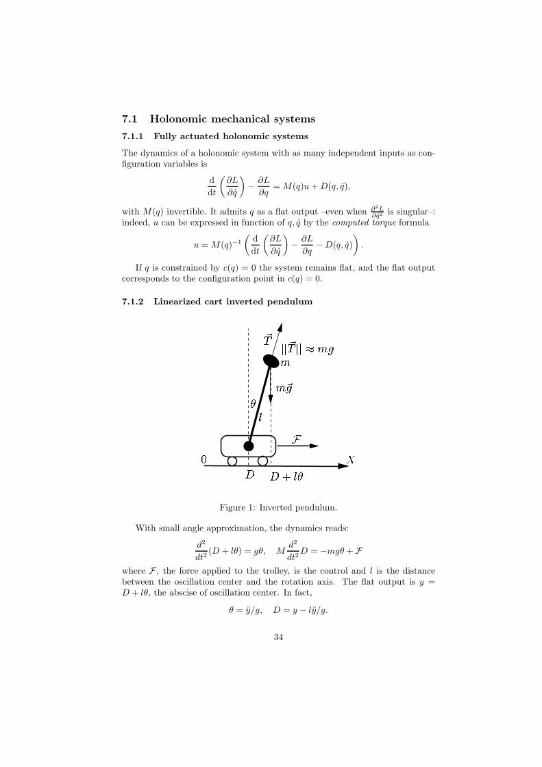
Figure 1: Inverted pendulum.

With small angle approximation, the dynamics reads:

d2

dt2(D + lθ) = gθ, M

d2

dt2D = −mgθ + F

where F , the force applied to the trolley, is the control and l is the distancebetween the oscillation center and the rotation axis. The flat output is y =D + lθ, the abscise of oscillation center. In fact,

θ = y/g, D = y − ly/g.

34

The high gain feedback (u as position set-point)

F = −Mk1D −Mk2(D − u)

with k1 ≈ 10/τ , k2 ≈ 10/τ2 (τ =√l/g), yields the following slow dynamics:

d2

dt2(y) = g(y − u)/l =

y − u

τ2.

The simple feedback

u = −y − τ2yr(t) + τ(y − yr(t)) + (y − yr(t))

ensure the tracking of t → yr(t).This system is not feedback linearizable for large angle thus itis not flat

(single input case).

7.1.3 The double inverted pendulum

Figure 2: The double inverted pendulum.

Take two identical homogeneous beam over a trolley whose position D is

35

directly controlled. Under small angle approximations, the dynamics reads

θ1 =y(2)

g− ly(4)

3g2

θ2 =y(2)

g+ly(4)

9g2

D = y − 3536lθ1 − 7

12lθ2

= y − 14ly(2)

9g+

7l2y(4)

27g2.

where y is the flat output.

7.1.4 Planar rigid body with forces

Figure 3: Planar rigid solid controlled by two body fixed forces.

Consider a planar rigid body moving in a vertical plane under the influenceof gravity and controlled by two forces having lines of action that are fixed withrespect to the body and intersect at a single point (see figure 3) (see [111]).The force are denoted by F1 and F2. Their directions, e1 and e2, are fixedwith respect to the solid. These forces are applied at S1 and S2 points that arefixed with respect to the solid. We assume that these forces are independent, i.e.,when S1 = S2 their direction are not the same. We exclude the case S1 = S2 = Gsince the system is not controllable (kinetic momentum is invariant).

Set G the mass center and θ the orientation of the solid. Denote by k theunitary vector orthogonal to the plane. m is the mass and J the inertia withrespect to the axis passing through G and of direction k. g is the gravity.

Dynamics read

mG = F1 + F2 +mg

Jθk =−−→GS1 ∧ F1 +

−−→GS2 ∧ F2.

36

As shown on figure 3, flat output P is Huyghens oscillation center when thecenter of rotation is the intersection Q of the straight lines (S1, e1) and (S2, e2):

P = Q+

√1 +

J

ma2

−−→QG.

with a = QG. Notice that when e1 and e2 are co-linear Q is sent to ∞ and Pcoincides with G. Point P is the only point such that P − g is colinear to thedirection PG, i.e, gives θ.

This example has some practical importance. The PVTOL system, thegantry crane and the robot 2kπ (see below) are of this form, as is the simplifiedplanar ducted fan [75]. Variations of this example can be formed by changingthe number and type of the inputs [71].

7.1.5 The rocket

Figure 4: a rocket and it flat output P .

Other examples are possible in the 3-dimensional space with rigid bodyadmitting symmetries. Take, e.g., the rocket of figure 4. Its equations are (noaero-dynamic forces)

mG = F +mg

Jd

dt(b ∧ b) = −−→

SG ∧ F

where b =−→SG/SG and

P = S +√SG2 + J/m b.

It is easy to see that P − g is co-linear to the direction b.

37

7.1.6 PVTOL aircraft

A simplified Vertical Take Off and Landing aircraft moving in a vertical Plane [34]can be described by

x = −u1 sin θ + εu2 cos θz = u1 cos θ + εu2 sin θ − 1

θ = u2.

A flat output is y = (x − ε sin θ, z + ε cos θ), see [58] more more details and adiscussion in relation with unstable zero dynamics.

7.1.7 2kπ the juggling robot [47]

laboratoryframe

O

Pendulum

g S

motor

motor

motor

θ1

θ2

θ 3

Figure 5: the robot 2kπ.

The robot 2kπ is developed at Ecole des Mines de Paris and consists ofa manipulator carrying a pendulum, see figure 5. There are five degrees offreedom (dof’s): 3 angles for the manipulator and 2 angles for the pendulum.The 3 dof’s of the manipulator are actuated by electric drives, while the 2 dof’sof the pendulum are not actuated.

This system is typical of underactuated, nonlinear and unstable mechanicalsystems such as the PVTOL [57], Caltech’s ducted fan [64, 59], the gantrycrane [22], Champagne flyer [46]. As shown in [53, 22, 59] the robot 2kπ is flat,with the center of oscillation of the pendulum as a flat output. Let us recallsome elementary facts

38

The cartesian coordinates of the suspension point S of the pendulum can beconsidered here as the control variables : they are related to the 3 angles of themanipulator θ1, θ2, θ3 via static relations. Let us concentrated on the pendulumdynamics. This dynamics is similar to the ones of a punctual pendulum withthe same mass m located at point H , the oscillation center (Huygens theorem).Denoting by l = ‖SH‖ the length of the isochronous punctual pendulum, New-ton equation and geometric constraints yield the following differential-algebraicsystem (T is the tension, see figure 6):

mH = T +mg, SH ∧ T = 0, ‖SH‖ = l.

If, instead of setting t → S(t), we set t → H(t), then T = m(H − g). S islocated at the intersection of the sphere of center H and radius l with the linepassing through H of direction H − g:

S = H ± 1‖H − g‖ (H − g).

These formulas are crucial for designing a control law steering the pendulumfrom the lower equilibrium to the upper equilibrium, and also for stabilizing thependulum while the manipulator is moving around [47].

Figure 6: the isochronous pendulum.

7.1.8 Towed cable systems [70, 59]

This system consists of an aircraft flying in a circular pattern while towinga cable with a tow body (drogue) attached at the bottom. Under suitableconditions, the cable reaches a relative equilibrium in which the cable maintainsits shape as it rotates. By choosing the parameters of the system appropriately,it is possible to make the radius at the bottom of the cable much smaller thanthe radius at the top of the cable. This is illustrated in Figure 7.

The motion of the towed cable system can be approximately representedusing a finite element model in which segments of the cable are replaced byrigid links connected by spherical joints. The forces acting on the segment(tension, aerodynamic drag and gravity) are lumped and applied at the end of

39

Figure 7: towed cable system and finite link approximate model.

each rigid link. In addition to the forces on the cable, we must also considerthe forces on the drogue and the towplane. The drogue is modeled as a sphereand essentially acts as a mass attached to the last link of the cable, so thatthe forces acting on it are included in the cable dynamics. The external forceson the drogue again consist of gravity and aerodynamic drag. The towplane isattached to the top of the cable and is subject to drag, gravity, and the forceof the attached cable. For simplicity, we simply model the towplane as a pureforce applied at the top of the cable. Our goal is to generate trajectories for thissystem that allow operation away from relative equilibria as well as transitionbetween one equilibrium point and another. Due to the high dimension of themodel for the system (128 states is typical), traditional approaches to solvingthis problem, such as optimal control theory, cannot be easily applied. However,it can be shown that this system is differentially flat using the position of thebottom of the cable Hn as the differentially flat output. See [70] for a morecomplete description and additional references.

Assume no friction and only gravity. Then, as for the pendulum of 2kπ, wehave

Hn−1 = Hn +1

‖mnHn −mng‖(mnHn −mng)

where mn is the mass of link n. Newton equation for link n − 1 yields (with

40

obvious notations)

Hn−2 = Hn−1 +(mnHn +mn−1Hn−1 − (mn +mn−1)g)

‖mnHn +mn−1Hn−1 − (mn +mn−1)g‖.

More generally, we have at link i

Hi−1 = Hi +1

‖∑ni mk(Hk − g)‖

(n∑i

mk(Hk − g)

).

These relations imply that S is function of Hn and its time derivatives up to order 2n.Thus Hn is the flat output.

7.1.9 Gantry crane [22, 51, 49]

A direct application of Newton’s laws provides the implicit equations of motion

mx = −T sin θ x = R sin θ +D

mz = −T cos θ +mg z = R cos θ,

where x, z, θ are the configuration variables and T is the tension in the cable. Thecontrol inputs are the trolley position D and the cable length R. This system is flat,with the position (x, z) of the load as a flat output.

7.1.10 Conventional aircraft

A conventional aircraft is flat, provided some small aerodynamic effects are neglected,with the coordinates of the center of mass and side-slip angle as a flat output. See [53]for a detailed study.

7.1.11 Satellite with two controls

We end this section with a system which is not known to be flat for generic parametervalue but still enjoys the weaker property of being orbitally flat [20]. Consider with [6]a satellite with two control inputs u1, u2 described by

ω1 = u1

ω2 = u2

ω3 = aω1ω2

ϕ = ω1 cos θ + ω3 sin θ

θ = (ω1 sin θ − ω3 cos θ) tanϕ+ ω2

ψ =(ω3 cos θ − ω1 sin θ)

cosϕ,

(24)

where a = (J1 − J2)/J3 (Ji are the principal moments of inertia); physical senseimposes |a| ≤ 1. Eliminating u1, u2 and ω1, ω2 by

ω1 =ϕ− ω3 sin θ

cos θand ω2 = θ + ψ sinϕ

41

yields the equivalent system

ω3 = a(θ + ψ sinϕ)ϕ− ω3 sin θ

cos θ(25)

ψ =ω3 − ϕ sin θ

cosϕ cos θ. (26)

But this system is in turn equivalent to

cos θ(ψ cosϕ− (1 + a)ψϕ sinϕ

)+ sin θ

(ϕ+ aψ2 sinϕ cosϕ

)+ θ(1 − a)(ϕ cos θ − ψ sin θ cosϕ) = 0

by substituting ω3 = ψ cosϕ cos θ + ϕ sin θ in (25).When a = 1, θ can clearly be expressed in function of ϕ,ψ and their derivatives.

We have proved that (24) is flat with (ϕ,ψ) as a flat output. A similar calculation canbe performed when a = −1.

When |a| < 1, whether (24) is flat is unknown. Yet, it is orbitally flat [93]. To seethat, rescale time by σ = ω3; by the chain rule x = σx′ whatever the variable x, where′ denotes the derivation with respect to σ. Setting then

ω1 := ω1/ω3, ω2 := ω2/ω3, ω3 := −1/aω3,

and eliminating the controls transforms (24) into

ω′3 = ω1ω2

ϕ′ = ω1 cos θ + sin θ

θ′ = (ω1 sin θ − cos θ) tanϕ+ ω2

ψ′ =(cos θ − ω1 sin θ)

cosϕ.

The equations are now independent of a. This implies the satellite with a = 1 isorbitally equivalent to the satellite with a = 1. Since it is flat when a = 1 it isorbitally flat when a = 1, with (ϕ,ψ) as an orbitally flat output.

7.2 Nonholonomic mechanical systems

Many mobile robots such as considered in [7, 73, 108] admit the same structure. Theyare flat and the flat output corresponds to the Cartesian coordinates of a specialpoint. Starting from the classical n-trailer systems [98, 22, 97, 18] we show that, whenn, the number of trailers, tends to infinity the system tends to a trivial delay system,the non-holonomic snake. Invariance with respect to rotations and translations makevery natural the use of Frenet formulae and curve parameterization with respect toarc length instead of time (see [59, 99] for relations between flatness and physicalsymmetries) . The study of such systems gives us the opportunity to recall linkswith an old problem stated by Hilbert [35] and investigated by Cartan [8], on Pfaffiansystems, Goursat normal forms and (absolute) equivalence.

7.2.1 The car

The rolling without slipping conditions yield (see figure 8 for the notations)

x = v cos θy = v sin θ

θ =v

ltanϕ

(27)

42

Figure 8: kinematic of a car.

where v, the velocity, and ϕ, the steering angle are the two controls. These equationsmean geometrically that the angle θ gives the direction of the tangent to the curvefollowed by P , the point of coordinates (x, y), and that tanϕ/l corresponds to thecurvature of this curve:

v = ±‖P‖,(

cos θsin θ

)= P /v, tanϕ = l det(P P )/v

√|v|.

There is thus a one to one correspondence between arbitrary smooth curves and thesolutions of (27). It provides, as shown in [22], a very simple algorithm to steer thecar from on a configuration to another one.

7.2.2 Car with n-trailers [22]

Figure 9: car with n trailers.

Take the single car here above and hitch, as display on figure 9, n trailers. Theresulting system still admits two control: the velocity of the car v and the steeringangle φ. As for the single car, modelling is based on the rolling without slippingconditions.

There is a one to one correspondence between smooth curves of arbitrary shapesand the system trajectories. It suffices to consider the curve followed by Pn, the

43

cartesian position of the last trailer. It is not necessary to write down explicitly thesystem equations in the state-space form as (27). Just remember that the kinematicconstraints say that the velocity of each trailer (more precisely of the middle of itswheel axle) is parallel to the direction of its hitch.

Figure 10: case n = 1.

Take n = 1 and have a look at figure 10. Assume that the curve C followed byP1 is smooth. Take s → P (s) an arc length parameterization. Then P1 = P (s), θ1 isthe angle of τ , the unitary tangent vector to C. Since P0 = P + d1τ derivation withrespect to s provides

d

dsP0 = τ + d1κν

with (τ , ν) the Frenet frame of C and κ its curvature. Thusd

dsP0 = 0 is tangent to

C0, the curve followed by P0. This curve is necessary smooth and

tan(θ0 − θ1) = d1κ, τ0 =1√

1 + (d1κ)2(τ + d1κν).

Derivation with respect to s0, (ds0 =√

1 + (d1κ)2 ds) yields the steering angle φ :

tanφ = d0κ0 = d01√

1 + (d1κ)2

(κ+

d1

1 + (d1κ)2dκ

ds

).

The car velocity v is then given by

v(t) =√

1 + d21κ

2(s(t)) s(t)

for any C1 time function, t → s(t). Notice that φ and θ0 − θ1 always remain in] − π/2, π/2[. These computations prove the one to one correspondence between the

44

system trajectories respecting φ and θ0 − θ1 in ]−π/2, π/2[, and regular planar curvesof arbitrary shape with an arbitrary C1 time parameterization.

The case n > 1 is just a direct generalization. The correspondence between arbi-trary smooth curves s → P (s) (tangent τ , curvature κ) with a C1 time parameteriza-tion t → s(t) is then defined by a smooth invertible map

R2 × S

1 × Rn+2 → R

2 × S1×] − π/2, π/2[n+1×R(

P,τ, κ, dκds, . . . , dnκ

dsn , s)

→ (Pn, θn, θn − θn−1, . . . , θ1 − θ0, φ, v)

where v is the car velocity. More details are given in [22].With such a correspondence, motion planning reduces to a trivial problem: to find

a smooth curve with prescribed initial and final positions, tangents, curvatures κ andcurvature derivatives, diκ/dsi, i = 1, . . . , n.

7.2.3 The general one-trailer system [98]

Figure 11: car with one trailer.

This nonholonomic system is displayed on figure 11: here the trailer is not directlyhitched to the car at the center of the rear axle, but more realistically at a distance aof this point. The equations are

x = cosα vy = sinα v

α =1

ltanϕ v

β =1

b

(al

tanϕ cos(α− β) − sin(α− β))v.

(28)

Controls are the car velocity v and the steering angle ϕ.There still exists a one to one correspondence between the trajectories of (28) and

arbitrary smooth curves with a C1 time parameterization. Such curves are followedby the point P (see figure 11) of coordinates

X = x+ b cos β + L(α− β)b sin β − a sinα√

a2 + b2 − 2ab cos(α− β)

Y = y + b sin β + L(α− β)a cosα− b cos β√

a2 + b2 − 2ab cos(α− β)

(29)

45

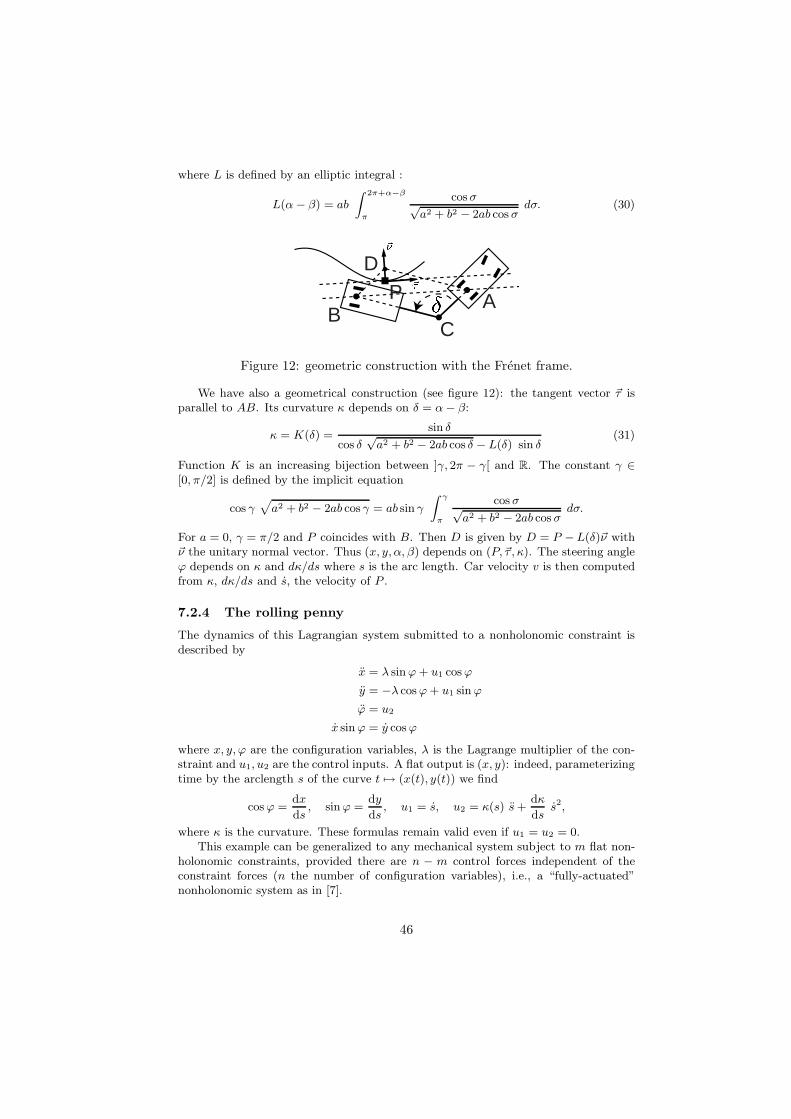
where L is defined by an elliptic integral :

L(α− β) = ab

∫ 2π+α−β

π

cosσ√a2 + b2 − 2ab cos σ

dσ. (30)

BC

APD

Figure 12: geometric construction with the Frenet frame.

We have also a geometrical construction (see figure 12): the tangent vector τ isparallel to AB. Its curvature κ depends on δ = α− β:

κ = K(δ) =sin δ

cos δ√a2 + b2 − 2ab cos δ − L(δ) sin δ

(31)

Function K is an increasing bijection between ]γ, 2π − γ[ and R. The constant γ ∈[0, π/2] is defined by the implicit equation

cos γ√a2 + b2 − 2ab cos γ = ab sin γ

∫ γ

π

cos σ√a2 + b2 − 2ab cos σ

dσ.

For a = 0, γ = π/2 and P coincides with B. Then D is given by D = P −L(δ)ν withν the unitary normal vector. Thus (x, y, α, β) depends on (P,τ , κ). The steering angleϕ depends on κ and dκ/ds where s is the arc length. Car velocity v is then computedfrom κ, dκ/ds and s, the velocity of P .

7.2.4 The rolling penny

The dynamics of this Lagrangian system submitted to a nonholonomic constraint isdescribed by

x = λ sinϕ+ u1 cosϕ

y = −λ cosϕ+ u1 sinϕ

ϕ = u2

x sinϕ = y cosϕ

where x, y, ϕ are the configuration variables, λ is the Lagrange multiplier of the con-straint and u1, u2 are the control inputs. A flat output is (x, y): indeed, parameterizingtime by the arclength s of the curve t → (x(t), y(t)) we find

cosϕ =dx

ds, sinϕ =

dy

ds, u1 = s, u2 = κ(s) s+

dκ

dss2,

where κ is the curvature. These formulas remain valid even if u1 = u2 = 0.This example can be generalized to any mechanical system subject to m flat non-

holonomic constraints, provided there are n − m control forces independent of theconstraint forces (n the number of configuration variables), i.e., a “fully-actuated”nonholonomic system as in [7].

46

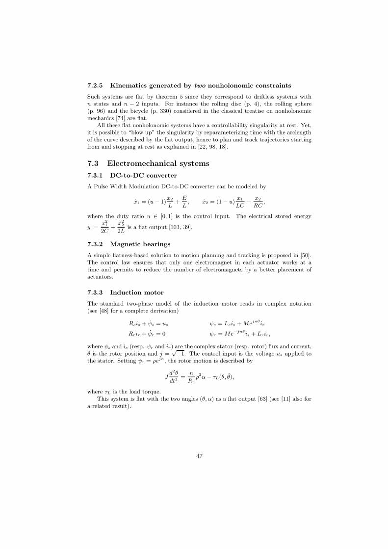
7.2.5 Kinematics generated by two nonholonomic constraints

Such systems are flat by theorem 5 since they correspond to driftless systems withn states and n − 2 inputs. For instance the rolling disc (p. 4), the rolling sphere(p. 96) and the bicycle (p. 330) considered in the classical treatise on nonholonomicmechanics [74] are flat.

All these flat nonholonomic systems have a controllability singularity at rest. Yet,it is possible to “blow up” the singularity by reparameterizing time with the arclengthof the curve described by the flat output, hence to plan and track trajectories startingfrom and stopping at rest as explained in [22, 98, 18].

7.3 Electromechanical systems

7.3.1 DC-to-DC converter

A Pulse Width Modulation DC-to-DC converter can be modeled by

x1 = (u− 1)x2

L+E

L, x2 = (1 − u)

x1

LC− x2

RC,

where the duty ratio u ∈ [0, 1] is the control input. The electrical stored energy

y :=x2

1

2C+x2

2

2Lis a flat output [103, 39].

7.3.2 Magnetic bearings

A simple flatness-based solution to motion planning and tracking is proposed in [50].The control law ensures that only one electromagnet in each actuator works at atime and permits to reduce the number of electromagnets by a better placement ofactuators.

7.3.3 Induction motor

The standard two-phase model of the induction motor reads in complex notation(see [48] for a complete derivation)

Rsis + ψs = us ψs = Lsis +Mejnθir

Rrir + ψr = 0 ψr = Me−jnθis + Lrir,

where ψs and is (resp. ψr and ir) are the complex stator (resp. rotor) flux and current,θ is the rotor position and j =

√−1. The control input is the voltage us applied tothe stator. Setting ψr = ρejα, the rotor motion is described by

Jd2θ

dt2=

n

Rrρ2α− τL(θ, θ),

where τL is the load torque.This system is flat with the two angles (θ, α) as a flat output [63] (see [11] also for

a related result).

47

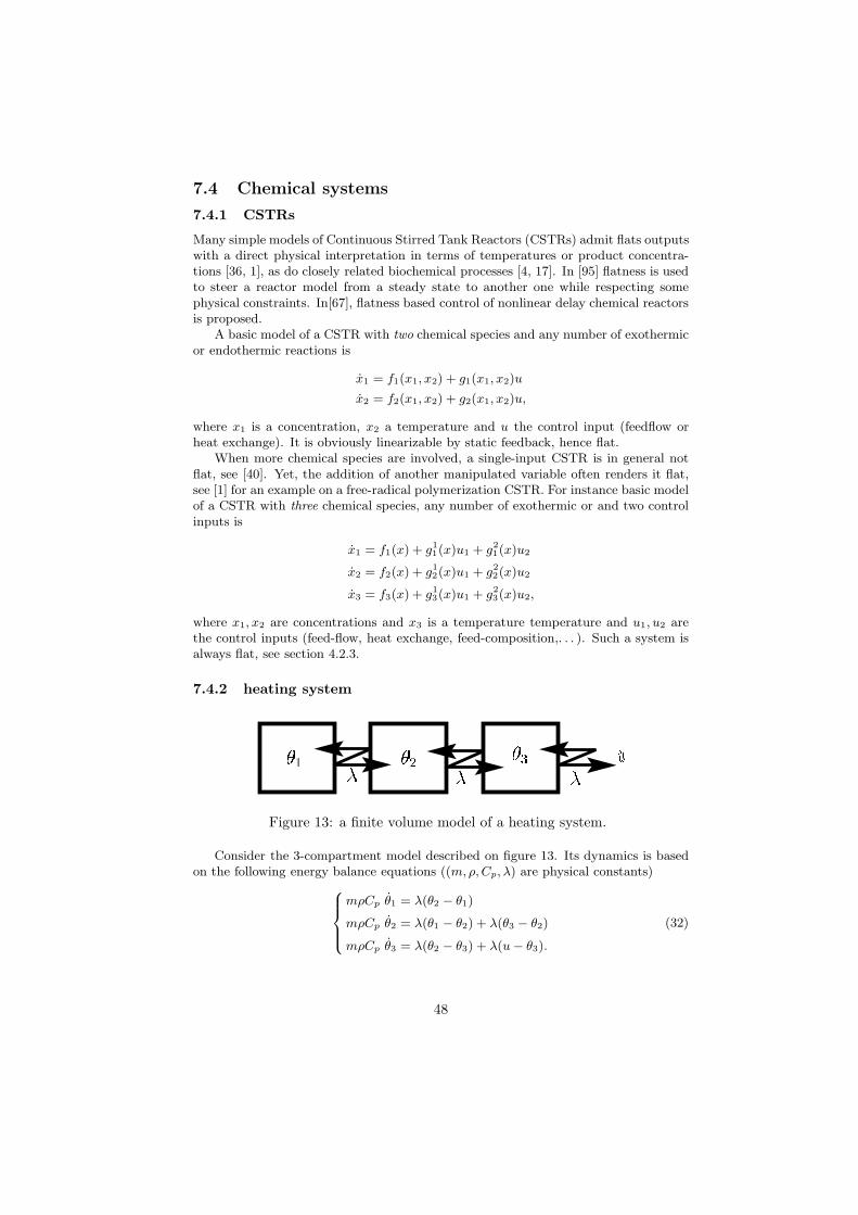
7.4 Chemical systems

7.4.1 CSTRs

Many simple models of Continuous Stirred Tank Reactors (CSTRs) admit flats outputswith a direct physical interpretation in terms of temperatures or product concentra-tions [36, 1], as do closely related biochemical processes [4, 17]. In [95] flatness is usedto steer a reactor model from a steady state to another one while respecting somephysical constraints. In[67], flatness based control of nonlinear delay chemical reactorsis proposed.

A basic model of a CSTR with two chemical species and any number of exothermicor endothermic reactions is

x1 = f1(x1, x2) + g1(x1, x2)u

x2 = f2(x1, x2) + g2(x1, x2)u,

where x1 is a concentration, x2 a temperature and u the control input (feedflow orheat exchange). It is obviously linearizable by static feedback, hence flat.

When more chemical species are involved, a single-input CSTR is in general notflat, see [40]. Yet, the addition of another manipulated variable often renders it flat,see [1] for an example on a free-radical polymerization CSTR. For instance basic modelof a CSTR with three chemical species, any number of exothermic or and two controlinputs is

x1 = f1(x) + g11(x)u1 + g2

1(x)u2

x2 = f2(x) + g12(x)u1 + g2

2(x)u2

x3 = f3(x) + g13(x)u1 + g2

3(x)u2,

where x1, x2 are concentrations and x3 is a temperature temperature and u1, u2 arethe control inputs (feed-flow, heat exchange, feed-composition,. . . ). Such a system isalways flat, see section 4.2.3.

7.4.2 heating system

Figure 13: a finite volume model of a heating system.

Consider the 3-compartment model described on figure 13. Its dynamics is basedon the following energy balance equations ((m,ρ,Cp, λ) are physical constants)

mρCp θ1 = λ(θ2 − θ1)

mρCp θ2 = λ(θ1 − θ2) + λ(θ3 − θ2)

mρCp θ3 = λ(θ2 − θ3) + λ(u− θ3).

(32)

48

Its is obvious that this linear system is controllable with y = θ1 as Brunovsky output:it can be transformed via linear change of coordinates and linear static feedback intoy(3) = v.

Taking an arbitrary number n of compartments yields

mρCp θ1 = λ(θ2 − θ1)

mρCp θ2 = λ(θ1 − θ2) + λ(θ3 − θ2)

...

mρCp θi = λ(θi−1 − θi) + λ(θi+1 − θi)

...

mρCp θn−1 = λ(θn−2 − θn−1) + λ(θn − θn−1)

mρCp θn = λ(θn−1 − θn) + λ(u− θn).

(33)

y = θ1 remains the Brunovsky output: via linear change of coordinates and linearstatic feedback we have y(n) = v.

When n tends to infinity, m and λ tend to zeros as 1/n and (33) tends to theclassical heat equation where the temperature on the opposite side to u, i.e., y = θ(0, t),still plays a special role.

7.4.3 Polymerization reactor

Consider with [106] the reactor

Cm =Cmms

τ−(

1 + εµ1

µ1 +MmCm

)Cm

τ+Rm(Cm, Ci, Cs, T )

Ci = −ki(T )Ci + u2

Ciis

V−(

1 + εµ1

µ1 +MmCm

)Ci

τ

Cs = u2

Csis

V+Csms

τ−(

1 + εµ1

µ1 +MmCm

)Cs

τ

µ1 = −MmRm(Cm, Ci, Cs, T ) −(

1 + εµ1

µ1 +MmCm

)µ1

τ

T = φ(Cm, Ci, Cs, µ1, T ) + α1Tj

Tj = f6(T, Tj) + α4u1,

where u1, u2 are the control inputs and Cmms, Mm, ε, τ, Ciis

, Csms, Csis

, V , α1,α4 are constant parameters. The functions Rm, ki, φ and f6 are not well-known andderive from experimental data and semi-empirical considerations, involving kineticlaws, heat transfer coefficients and reaction enthalpies.

The polymerization reactor is flat whatever the functions Rm, ki, φ, f6 and admits(Csis

Ci − CiisCs, MmCm + µ1) as a flat output [96].

8 Infinite dimension “flat” systems

The idea underlying equivalence and flatness –a one-to-one correspondence betweentrajectories of systems– is not restricted to control systems described by ordinary

49

differential equations. It can be adapted to delay differential systems and to par-tial differential equations with boundary control. Of course, there are many moretechnicalities and the picture is far from clear. Nevertheless, this new point of viewseems promising for the design of control laws. In this section, we sketch some recentdevelopments in this direction.

8.1 Delay systems

Consider for instance the simple differential delay system

x1(t) = x2(t), x2(t) = x1(t) − x2(t) + u(t− 1).

Setting y(t) := x1(t), we can clearly explicitly parameterize its trajectories by

x1(t) = y(t), x2(t) = y(t), u(t) = y(t+ 1) + y(t+ 1) − y(t+ 1).

In other words, y(t) := x1(t) plays the role of a“flat” output. This idea is investigatedin detail in [66], where the class of δ-free systems is defined (δ is the delay operator).More precisely, [66, 68] considers linear differential delay systems

M(d/dt, δ)w = 0

where M is a (n − m) × n matrix with entries polynomials in d/dt and δ and w =(w1, . . . , wn) are the system variables. Such a system is said to be δ-free if it can berelated to the “free” system y = (y1, . . . , ym) consisting of arbitrary functions of timeby

w = P (d/dt, δ, δ−1)y

y = Q(d/dt, δ, δ−1)w,

where P (resp. Q) is a n×m (resp. m×n ) matrix the entries of which are polynomialin d/dt, δ and δ−1.

Many linear delay systems are δ-free. For example, x(t) = Ax(t) + Bu(t − 1),(A,B) controllable, is δ-free, with the Brunovski output of x = Ax+Bv as a “δ-free”output.

The following systems, commonly used in process control,

zi(s) =m∑

j=1

Kj

i exp(−sδji )

1 + τ ji s

uj(s), i = 1, . . . p

(s Laplace variable, gains Kji , delays δj

i and time constants τ ji between uj and zi) are

δ-free [79]. Other interesting examples of δ-free systems arise from partial differentialequations:

Example 16 (Torsion beam system). The torsion motion of a beam (figure 14)can be modeled in the linear elastic domain by

∂2t θ(x, t) = ∂2

xθ(x, t), x ∈ [0, 1]

∂xθ(0, t) = u(t)

∂xθ(1, t) = ∂2t θ(1, t),

50

where θ(x, t) is the torsion of the beam and u(t) the control input. From d’Alembert’sformula, θ(x, t) = φ(x+ t) + ψ(x− t), we easily deduce

2θ(t, x) = y(t+ x− 1) − y(t− x+ 1) + y(t+ x− 1) + y(t− x+ 1)

2u(t) = y(t+ 1) + y(t− 1) − y(t+ 1) + y(t− 1),

where we have set y(t) := θ(1, t). This proves the system is δ-free with θ(1, t) as a“δ-flat” output. See [69, 27, 30] for details and an application to motion planning.

u(t)

θ(x, t)y (t) = θ(1, t)

0

1

x

Figure 14: torsion of a flexible beam

Many examples of delay systems derived from the 1D-wave equation can be treatedvia such techniques (see [16] for tank filled with liquid, [26] for the telegraph equationand [80] for two physical examples with delay depending on control).

Figure 15: the homogeneous chain without any load.

51

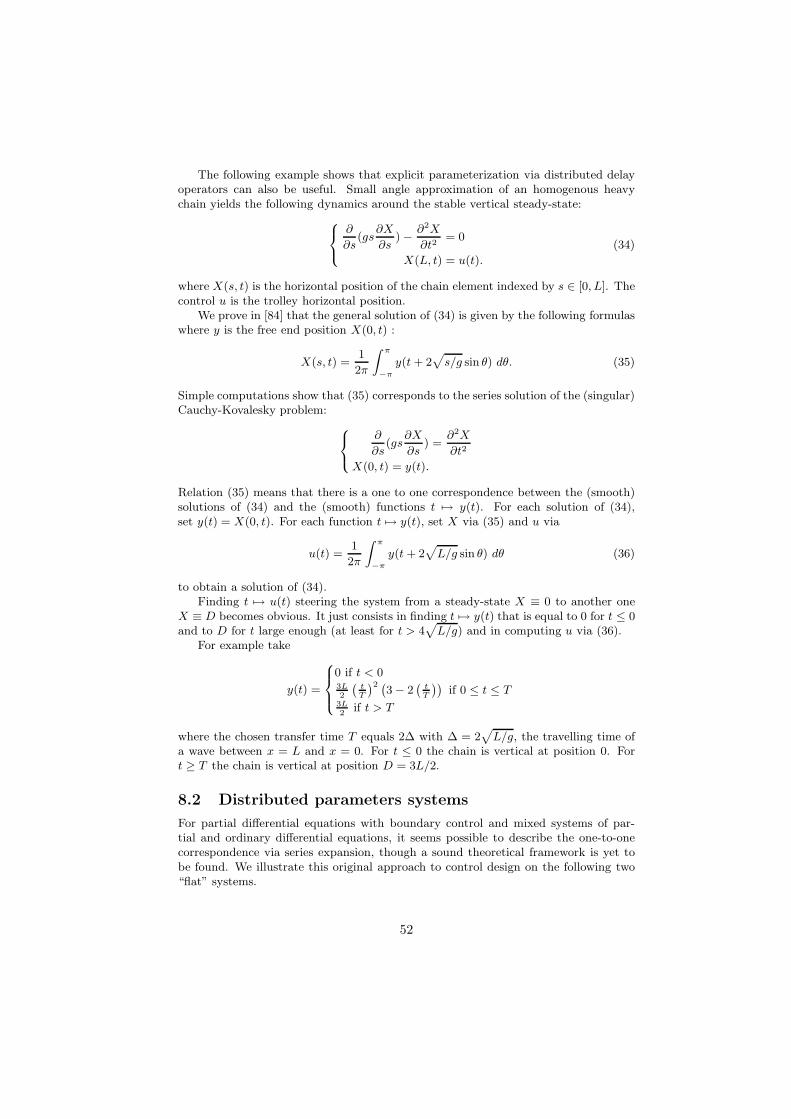
The following example shows that explicit parameterization via distributed delayoperators can also be useful. Small angle approximation of an homogenous heavychain yields the following dynamics around the stable vertical steady-state:

∂

∂s(gs

∂X

∂s) − ∂2X

∂t2= 0

X(L, t) = u(t).

(34)

where X(s, t) is the horizontal position of the chain element indexed by s ∈ [0, L]. Thecontrol u is the trolley horizontal position.

We prove in [84] that the general solution of (34) is given by the following formulaswhere y is the free end position X(0, t) :

X(s, t) =1

2π

∫ π

−π

y(t+ 2√s/g sin θ) dθ. (35)

Simple computations show that (35) corresponds to the series solution of the (singular)Cauchy-Kovalesky problem:

∂

∂s(gs

∂X

∂s) =

∂2X

∂t2

X(0, t) = y(t).

Relation (35) means that there is a one to one correspondence between the (smooth)solutions of (34) and the (smooth) functions t → y(t). For each solution of (34),set y(t) = X(0, t). For each function t → y(t), set X via (35) and u via

u(t) =1

2π

∫ π

−π

y(t+ 2√L/g sin θ) dθ (36)

to obtain a solution of (34).Finding t → u(t) steering the system from a steady-state X ≡ 0 to another one

X ≡ D becomes obvious. It just consists in finding t → y(t) that is equal to 0 for t ≤ 0and to D for t large enough (at least for t > 4

√L/g) and in computing u via (36).

For example take

y(t) =

0 if t < 03L2

(tT

)2 (3 − 2

(tT

))if 0 ≤ t ≤ T

3L2

if t > T

where the chosen transfer time T equals 2∆ with ∆ = 2√L/g, the travelling time of

a wave between x = L and x = 0. For t ≤ 0 the chain is vertical at position 0. Fort ≥ T the chain is vertical at position D = 3L/2.

8.2 Distributed parameters systems

For partial differential equations with boundary control and mixed systems of par-tial and ordinary differential equations, it seems possible to describe the one-to-onecorrespondence via series expansion, though a sound theoretical framework is yet tobe found. We illustrate this original approach to control design on the following two“flat” systems.

52

Example 17 (Heat equation). Consider as in [45] the linear heat equation

∂tθ(x, t) = ∂2xθ(x, t), x ∈ [0, 1] (37)

∂xθ(0, t) = 0 (38)

θ(1, t) = u(t), (39)

where θ(x, t) is the temperature and u(t) is the control input.

We claim thaty(t) := θ(0, t)

is a “flat” output. Indeed, the equation in the Laplace variable s reads

sθ(x, s) = θ′′(x, s) with θ′(0, s) = 0, θ(1, s) = u(s)

( ′ stands for ∂x and ˆ for the Laplace transform), and the solution is clearly θ(x, s) =cosh(x

√s)u(s)/ cosh(

√s). As θ(0, s) = u(s)/ cosh(

√s), this implies

u(s) = cosh(√s) y(s) and θ(x, s) = cosh(x

√s) y(s).

Since cosh√s =

∑+∞i=0 s

i/(2i)!, we eventually get

θ(x, t) =+∞∑i=1

x2i y(i)(t)

(2i)!(40)

u(t) =

+∞∑i=1

y(i)(t)

(2i)!. (41)

In other words, whenever t → y(t) is an arbitrary function (i.e., a trajectory of thetrivial system y = v), t → (

θ(x, t), u(t))

defined by (40)-(41) is a (formal) trajectoryof (37)–(39), and vice versa. This is exactly the idea underlying the definition offlatness. Notice these calculations have been known for a long time, see [109, pp. 588and 594].

To make the statement precise, we now turn to convergence issues. On the onehand, t → y(t) must be a smooth function such that

∃ K,M > 0, ∀i ≥ 0,∀t ∈ [t0, t1], |y(i)(t)| ≤M(Ki)2i

to ensure the convergence of the series (40)-(41).On the other hand t → y(t) cannot in general be analytic. Indeed, if the system is

to be steered from an initial temperature profile θ(x, t0) = α0(x) at time t0 to a finalprofile θ(x, t1) = α1(x) at time t1, equation (37) implies

∀t ∈ [0, 1], ∀i ≥ 0, y(i)(t) = ∂itθ(0, t) = ∂2i

x θ(0, t),

and in particular

∀i ≥ 0, y(i)(t0) = ∂2ix α0(0) and y(i)(t1) = ∂2i

x α1(1).

If for instance α0(x) = c for all x ∈ [0, 1] (i.e., uniform temperature profile), theny(t0) = c and y(i)(t0) = 0 for all i ≥ 1, which implies y(t) = c for all t when thefunction is analytic. It is thus impossible to reach any final profile but α1(x) = c forall x ∈ [0, 1].

53

Smooth functions t ∈ [t0, t1] → y(t) that satisfy

∃ K,M > 0, ∀i ≥ 0, |y(i)(t)| ≤M(Ki)σi

are known as Gevrey-Roumieu functions of order σ [91] (they are also closely related toclass S functions [32]). The Taylor expansion of such functions is convergent for σ ≤ 1and divergent for σ > 1 (the larger σ is, the “more divergent” the Taylor expansion is). Analytic functions are thus Gevrey-Roumieu of order ≤ 1.

In other words we need a Gevrey-Roumieu function on [t0, t1] of order > 1 but ≤ 2,with initial and final Taylor expansions imposed by the initial and final temperatureprofiles. With such a function, we can then compute open-loop control steering thesystem from one profile to the other by the formula (40).

For instance, we steered the system from uniform temperature 0 at t = 0 to uniformtemperature 1 at t = 1 by using the function

R t → y(t) :=

0 if t < 0

1 if t > 1∫ t

0exp

(−1/(τ (1 − τ ))γ)dτ∫ 1

0exp

(−1/(τ (1 − τ ))γ)dτ

if t ∈ [0, 1],

with γ = 1 (this function is Gevrey-Roumieu functions of order 1+1/γ). The evolutionof the temperature profile θ(x, t) is displayed on figure 16 (the Matlab simulation isavailable upon request at rouchon@cas.ensmp.fr).

00.2

0.40.6

0.81

0

0.2

0.4

0.6

0.8

10

0.5

1

1.5

2

x t

thet

a

Figure 16: evolution of the temperature profile for t ∈ [0, 1].

54

Similar but more involved calculations with convergent series corresponding toMikunsinski operators are used in [28, 29] to control a chemical reactor and a flexiblerod modeled by an Euler-Bernoulli equation. For nonlinear systems, convergence issuesare more involved and are currently under investigation. Yet, it is possible to work–at least formally– along the same line.

Example 18 (Flexion beam system). Consider with [43] the mixed system

ρ∂2t u(x, t) = ρω2(t)u(x, t) − EI∂4

xu(x, t), x ∈ [0, 1]

ω(t) =Γ3(t) − 2ω(t) <u, ∂tu>(t)

Id+ <u, u>(t)

with boundary conditions

u(0, t) = ∂xu(0, t) = 0, ∂2xu(1, t) = Γ1(t), ∂3

xu(1, t) = Γ2(t),

where ρ,EI, Id are constant parameters, u(x, t) is the deformation of the beam, ω(t)is the angular velocity of the body and <f, g>(t) :=

∫ 1

0ρf(x, t)g(x, t)dx. The three

control inputs are Γ1(t), Γ2(t), Γ3(t).

We claim thaty(t) :=

(∂2

xu(0, t), ∂3xu(0, t), ω(t)

)is a “flat” output. Indeed, ω(t), Γ1(t), Γ2(t) and Γ3(t) can clearly be expressed interms of y(t) and u(x, t), which transforms the system into the equivalent Cauchy-Kovalevskaya form

EI∂4xu(x, t) = ρy2

3(t)u(x, t) − ρ∂2t u(x, t) and

u(0, t) = 0

∂xu(0, t) = 0

∂2xu(0, t) = y1(t)

∂3xu(0, t) = y2(t).

Set then formally u(x, t) =∑+∞

i=0 ai(t)xi

i!, plug this series into the above system and

identify term by term. This yields

a0 = 0, a1 = 0, a2 = y1, a3 = y2,

and the iterative relation ∀i ≥ 0, EIai+4 = ρy23ai − ρai. Hence for all i ≥ 1,

a4i = 0 a4i+2 =ρ

EI(y2

3a4i−2 − a4i−2)

a4i+1 = 0 a4i+3 =ρ

EI(y2

3a4i−1 − a4i−1).

There is thus a 1–1 correspondence between (formal) solutions of the system andarbitrary mappings t → y(t): the system is formally flat.

For recent results on nonlinear flexion systems see [101].

9 A catalog of infinite dimensional “flat systems”

9.1 Chemical reactor with a recycle loop

This example is borrowed to [100] where a catalogue of flat chemical systems is avail-able. Take the exothermic chemical reactor studied in [3] (one reaction A −→ B

55

Figure 17: A chemical reactor with a recycle loop.

involving two species, A and B) and add, as shown on figure 17, a recycle loop anda delay τQ in the cooling system. Under classical assumption the mass and energybalances read

x(t) = D(xF − x(t)) +DR(x(t− τR) − x(t)) − r(x(t), T (t))

T (t) = D(TF − T (t)) +DR(T (t− τR) − T (t)) + α r(x(t), T (t)) +Q(t− τQ).(42)

The concentration of A is denoted by x and the temperature by T . The control Q isproportional to the cooling duty. The constant parameter are : α (reaction enthalpy); D (dilution rate); xF and TF (feed composition and temperature).

The recycle dynamics is described here by a delay τR (plug flow without reactionnor diffusion). Denote by VR the volume of the recycle loop and FR the recyclevolumetric flow. Then τR = VR/FR. We will show that y = x(t) is the flat-output.

Assume that x(t) = y(t) is given. The mass balance (the first equation in (42))defines implicitly the temperature T as a function of y(t), y(t) and y(t− τR) :

T (t) = Θ(y(t), y(t), y(t− τR)).

The energy balance reads

Q(t− τQ) = T (t) −D(TF − T (t)) −DR(T (t− τR) − T (t)) − α r(y(t), T (t));

thus

Q(t) = T (t+ τQ) −D(TF − T (t+ τQ)) −DR(T (t− τR + τQ) − T (t+ τQ))

−α r(y(t+ τQ), T (t+ τQ)).

This means that Q(t) depends on y(t + τQ), y(t + τQ), y(t + τQ), y(t − τR + τQ),y(t− 2τR + τQ) et y(t− τR + τQ). Formally we have

Q(t) = Λ[y(t+ τQ), y(t+ τQ), y(t+ τQ), y(t− τR + τQ), y(t− 2τR + τQ),

y(t− τR + τQ)].

The value of Q(t) for t ∈ [0, t∗] depends on y(t) for t ∈ [−2τR + τQ, t∗ + τQ]. Tofind a control steering the system from one steady state to another one, take t → y(t)constant outside of [0, t∗]. Then the transition starts at t = −τQ for Q, at t = 0 forT and x. The new steady-state is reached at t = t∗ for x, at t = t∗ + τR for T andt = t∗ + 2τR − τQ for Q.

56

9.2 The nonholonomic snake

Figure 18: the non-holonomic snake, a car with an infinite number of smalltrailers.

When the number of trailers is large, it is natural, as displayed on figure 18, tointroduce the continuous approximation of the “non-holonomic snake”. The trailersare now indexed by a continuous variable l ∈ [0, L] and their positions are given by amap [0, L] l →M(l, t) ∈ R

2 satisfying the following partial differential equations:∥∥∥∥∂M∂l∥∥∥∥ = 1,

∂M

∂l∧ ∂M

∂t= 0.

The first equation says that l →M(l, t) is an arc length parameterization. The secondone is just the rolling without slipping conditions : velocity of trailer l is parallel tothe direction of the plan of its wheels, i.e., the tangent to the curve l → M(l, t). It isthen obvious that the general solution of this system is

M(l, t) = P (s(t)− l), l ∈ [0, L]

where P is the snake head and s → P (s) an arc length parameterization of the curvefollowed by P . Similarly,

M(l, t) = Q(s(t) + l), l ∈ [0, L]

where Q is the snake tail. It corresponds to the flat output of the finite dimensionalapproximation, the n-trailers system of figure 9, with n large and di = L/n. Deriva-tives up to order n are in the infinite case replaced by advances in the arc length scale.This results from the formal relation

Q(s+ l) =∑i≥0

Q(i)(s)li/i!

and the series truncation up to the first n terms. Nevertheless, M(l, t) = Q(s(t) + l)is much more simple to use in practice. When n is large, the series admit convergencetroubles for s → Q(s) smooth but not analytic.

When the number of trailers is large and the curvature radius 1/κ of s → Q(s) ismuch larger than the length of each small trailer, such infinite dimensional approxi-mation is valid. It reduces the dynamics to trivial delays. It is noteworthy that, inthis case, an infinite dimensional description yields to a much better reduced modelthan a finite dimensional description that gives complex nonlinear control models andalgorithms 1.

1The finite dimensional system does not require to be flat (trailer i can be hitched to traileri − 1 not directly at the center of its wheel axle, but more realistically at a positive distanceof this point [60]).

57

9.3 Nonlinear heavy chain systems

The nonlinear conservative model of an homogenous heavy chain with an end mass isthe following.

ρ∂2M

∂t2=

∂

∂s

(T∂M

∂s

)+ ρg∥∥∥∥∂M∂s

∥∥∥∥ = 1

M(L, t) = u(t)

T (0, t)∂M

∂s(0, t) = m

∂2M

∂t2(0, t) −mg.

(43)

where [0, L] s → M(s, t) ∈ R3 is an arc length parameterization of the chain and

T (s, t) > 0 is the tension. The control u is the position of the suspension point. If weuse

N(s, t) =

∫ s

0

M(σ, t) dσ

instead of M(s, t) (Backlund transformation) we have

ρ∂2N

∂t2= T (s, t)

∂2N

∂s2(s, t) − T (0, t)

∂2N

∂s2(0, t) + ρsg∥∥∥∥∂2N

∂s2

∥∥∥∥ = 1

∂N

∂s(L, t) = u(t)

T (0, t)∂2N

∂s2(0, t) = m

∂3N

∂t2∂s(0, t) −mg

N(0, t) = 0.

Assume that the load trajectory is given

t → y(t) =∂N

∂s(0, t).

Then (we take the positive branch)

T (s, t) =

∥∥∥∥ρ∂2N

∂t2(s, t) − (ρs+m)g +my(t)

∥∥∥∥and we have the Cauchy-Kovalevsky problem

∂2N

∂s2(s, t) =

1

T (s, t)

(ρ∂2N

∂t2(s, t) − (ρs+m)g +my(t)

)N(0, t) = 0

∂N

∂s(0, t) = y(t).

Formally, its series solution expresses in terms of y and its derivatives of infinite order.This could be problematic since y must be analytic and the series converge for s ≥ 0small enough.

58

We will see here below that the solution of the tangent linearization of this Cauchy-Kovalevsky system around the stable vertical steady-state can be expressed via ad-vances and delays of y. Such a formulation avoids series with y derivatives of arbitraryorders. For the nonlinear system here above, we conjecture a solution involving non-linear delays and advances of y.

9.4 Burger equation without diffusion [80]

0

0.5

1

1.5

0

0.2

0.4

0.6

0.8

11

1.5

2

2.5

3

3.5

4

Figure 19: A velocity described by Burger equation; transition from low velocityv ≡ 1 to a high velocity v ≡ 4 without shock.

The Burger equation represent the velocity flied in a one dimensional gas whereparticles have no interaction and have an inertial motion in a tube of length l:

∂v

∂t+ v

∂v

∂x= 0 x ∈ [0, 1]

v(0, t) = u(t). (44)

The field x → v(x, t) represents the velocity of the particles for x ∈ [0, l]. The controlis the input velocity u(t) > 0.

The output velocity is y(t) = v(l, t). Since the acceleration of each particle is zero,its velocity remains constant. Thus the particle coming out of the tube at time t hasvelocity equation to y(t). At time t − l/y(t) this particle enters the as tube in x = 0with velocity u(t− 1/y(t)). Thus

y(t) = u(t− 1/y(t)).

59

Similarly;u(t) = y(t+ 1/u(t)).

More generally :y(t) = v(t− (1 − x)/y(t), x) x ∈ [0, 1]

andu(t) = v(t+ x/u(t), x) x ∈ [0, 1].

Formally, we have a one to one correspondence between t → v( , t), solution of (44),and t → y(t). This correspondence is effective as soon as y > 0 is differentiable,t → t− (1 − x)/y(t) increasing for all x ∈ [0, l], i.e., for all t, y(t) > −y2(t).

This condition corresponds to smooth solution and avoid shocks and discontinuoussolution. It is then easy to find t → u(t) steering smoothly from a low velocityv( , 0) ≡ v1 > 0 to a high one v( , T ) ≡ v2 > v1 in a time T . Notice that the samecomputation remains valid for

vt + λ(v)vx = 0 x ∈ [0, l]v(0, t) = u(t).

The relations between y(t) = v(l, t), u and v becomes (see, e.g., [13][page 41]):

y(t) = u[t− 1/λ(y(t))], y(t) = v[t− (1 − x)/λ(y(t)), x].

9.5 Mixing processes

Example of figure 20 comes from [80], a system where delays depend on control. Usingthree tanks with base colors, the goal is to produce in the output tank a specifiedquantity and color.

Since the pipe volume are comparable to the output tank volume, delays appear.We assume plug flow in pipes α and β. Knowing the output tank quantities, t → Y =(Y1, Y2, Y3), it is possible to derived explicitly the three control u = (u1, u2, u3) andthe color profile in pipes α and β via Y and its time derivative Y . Notations are asfollows (see figure 20).

• a color (or composition) is a triplet (c1, c2, c3) with ∀i = 1, 2, 3 0 ≤ ci ≤ 1 andc1 + c2 + c3 = 1.

• bi = (δij)j=1,2,3 corresponds to base color in the input tank no i, i = 1, 2, 3.

• u = (u1, u2, u3)T : the output flow from the input tanks (the control).

• α = (α1, α2, 0)T : color at mixing node α.

• β = (β1, β2, β3)T : color at mixing node β.

• V : volume in the output tank.

• X = (X1,X2,X3): color in the output tank.

• Y = (Y1, Y2, Y3)T = (V.X1, V.X2, V.X3)

T the three holdups in output tank.Y1, Y2, Y3 are increasing time functions.

• Vα: volume of pipe α.

• Vβ : volume of pipe β.

60

α

β

α

β

node

node

Figure 20: colors mixing; variable delays are due to non negligible pipe volumesVα and Vβ .

61

Notice that

α1 + α2 = 1, β1 + β2 + β3 = 1, X1 +X2 +X3 = 1.

Balance equations provide u, α and β versus Y . Assume that t → σ(t) → Y (σ(t))is given: t → σ(t) is a smooth increasing time function and σ → Yi(σ) is positive,smooth and strictly increasing, i = 1, 2, 3. Computations start from the output andfinish at the input. The main steps are ( ′ stands for d/dσ):

1. solve (via , e.g., a Newton-like method) the scalar equation

3∑i=1

Yi(σβ) =

3∑i=1

Yi(σ(t)) + Vβ

with σβ as unknown.

2. solve, similarly

Y1(σα) + Y2(σα) = Y1(σβ) + Y2(σβ) + Vα

with σα as unknown.

3. set

α1(t) =Y ′

1(σα)

Y ′1(σα) + Y ′

2(σα), α2(t) = 1 − α1(t).

and

β(t) =

[Y ′

V ′

](sβ)

with V = Y1 + Y2 + Y3.

4. setui(t) = αi(t) (Y ′

1(σβ) + Y ′2(σβ)) V ′(σ(t)) σ(t) i = 1, 2

andu3(t) = V ′(σ(t)) σ(t) − u1(t) − u2(t)

Assume now that we have to produce a series of batches of prescribed volumesand colors defined by Qa = (Qa

1 , Qa2 , Q

a3), Qb = (Qb

1, Qb2, Q

b3), Q

c, . . . . We cannotflush pipes α and β between two batches. Define an increasing Y , t → σ → Yi as onfigure 21. The clock law t → σ(t) admits horizontal tangent at ta, tb, tc, . . . to ensuresmooth transitions between batches.

9.6 Flexible beam (Euler-Bernoulli) [2, 28]

Symbolic computations “ a la Heaviside” with s instead of ∂∂t

are here important. Wewill not develop the formal aspect with Mikusinski operational calculus as in [28]. Wejust concentrate on the computations. We have the following 1D modelling:

∂ttX = −∂xxxxX

X(0, t) = 0, ∂xX(0, t) = θ(t)

θ(t) = u(t) + k∂xxX(0, t)

∂xxX(1, t) = −λ∂ttxX(1, t)∂xxxX(1, t) = µ∂ttX(1, t)

62

Y

Figure 21: Batch scheduling via smooth flat output t → σ(t) → Y (σ(t)).

Figure 22: a flexible beam rotating around a control axle

63

where the control is the motor torque u, X(r, t) is the deformation profile, k, λ and µare physical parameters (t and r are in reduced scales).

We will show that the general solution expresses in term of an arbitrary C∞

function y (Gevrey order ≤ 2 for convergence):

X(x, t) =∑n≥0

(−1)n y(2n)(t)

(4n)!Pn(x) +

∑n≥0

(−1)n y(2n+2)(t)

(4n+ 4)!Qn(x) (45)

with ı =√−1,

Pn(x) =x4n+1

2(4n+ 1)+

(− )(1 − x+ ı)4n+1

2(4n+ 1)+ µ(1 − x+ ı)4n

and

Qn(x) =λµ

2(4n+ 4)(4n+ 3)(4n+ 2)

((− )(1 − x+ ı)4n+1 − x4n+1)

− λ(4n+ 4)(4n+ 3)(1 − x+ ı)4n+2

( and stand for real part and imaginary part). Notice that θ and u result from (45):it suffices to derive term by term.

We just show here how to get these formulas with λ = µ = 0 ( no inertia at thefree end r = 1, M = J = 0). The method remains unchanged in the general case. Thequestion is: how to get

X(x, t) =∑n≥0

y(2n)(t)(−1)n

(4n)!πn(x) (46)

with

πn(x) =x4n+1

2(4n+ 1)+

( −)(1 − x+ ı)4n+1

2(4n+ 1).

With the Laplace variable s, we have the ordinary differential system

X(4) = −s2Xwhere

X(0) = 0, X(2)(1) = 0, X(3)(1) = 0.

Derivatives are with respect to the space variable r and s is here a parameter. Thegeneral solution depends on an arbitrary constant, i.e., an arbitrary function of s, sincewe have 3 boundary conditions. With the 4 elementary solutions of X(4) = −s2X

C+(x) = (cosh((1 − x)√sξ) + cosh((1 − x)

√s/ξ))/2

C−(x) = (cosh((1 − x)√sξ) − cosh((1 − x)

√s/ξ))/(2ı)

S+(x) = (ı sinh((1 − x)√sξ) + sinh((1 − x)

√s/ξ))/(2ξ

√s)

S−(x) = ξ(ı sinh((1 − x)√sξ) − sinh((1 − x)

√s/ξ))/(2

√s)

where ξ = exp(ıπ/4), X reads

X(x) = aC+(x) + bC−(x) + cS+(x) + dS−(x).

64

The 3 boundary conditions provide 3 equations relating the constant a, b, c and d :

aC+(0) + bC−(0) + cS+(0) + dS−(0) = 0

sb = 0

sc = 0.

Thus b = c = 0 and we have just one relation between a and d

aC+(0) + dS−(0) = 0.

SinceC+(0) = (cosh(ξ

√s), S−(0) = (ξ sinh(ξ

√s/√s)

are entire functions of s very similar to cosh(√s) and sinh

√s/√s appearing for the

heat equation (37), we can associate to them two operators, algebraically independentand commuting,

δ+ = C+(0), δ− = S−(0).

They are in fact ultra-distributions belonging to the dual of Gevrey function of orderless than ≤ 2 and with a punctual support [32]. We have thus a module generated bytwo elements (a, d) satisfying δ+a+ δ−d = 0. This is a R[δ+, δ−]-module. This moduleis not free but δ+-free [66]:

a = δ−y, d = −δ+ywith y = −δ−1

+ d.The basis y plays the role of flat output since

X(x) = (S−(0)C+(x) − S−(x)C+(0))y.

Simple but tedious computations using hyperbolic trigonometry formulas yield thento

X(x) = −1

2[S−(x) + (S−(1 − x+ ı))]y.

The series of the entire function S− provides (46). We conjecture that the quantityy admits a physical sense as an explicit expression with integrals of X over r ∈ [0, 1](center of flexion).

9.7 Horizontal translation of the circular tank: the tum-bler [83]

Take the 2D wave equation corresponding, in the linear approximation, to the sur-face wave generated by the horizontal motions of a cylindric tank containing a fluid(linearized Saint-Venant equations (shallow water approximation)):

∂2ξ

∂t2= gh ∆ξ on Ω

g∇ξ · n = −D · n on ∂Ω

(47)

where Ω is the interior of a circle of radius R and of center D(t) ∈ R2, the control

(n is the normal to the boundary ∂Ω), h + ξ is the height of liquid, g is the gravity.A family of solutions of (47) is given by the following formulas ((r, θ) are the polarcoordinates)

ξ(r, θ, t) =1

π

√h

g

(∫ 2π

0

cosα[a(t− r cosα

c

)cos θ + b

(t− r cosα

c

)sin θ

]dα

)

65

and ((u, v) are the Cartesian coordinates of D)

u =1

π

∫ 2π

0

a

(t− R cosα

c

)cos2 α dα, v =

1

π

∫ 2π

0

b

(t− R cosα

c

)cos2 α dα

where t → (a(t), b(t)) ∈ R2 is an arbitrary smooth function.

9.8 Tubular reactor (convection/diffusion)

We recalled here [29, 100]. The controls are the input flux at z = 0 of mass and energy.

Figure 23: Adiabatic tubular reator.

It is then possible to parameterize trajectories versus the outflow concentrations x(l, t)and temperature T (l, t).

To simplify consider the tangent linearization around a steady-state. This givesthe following convection-diffusion system:

∂

∂t

[x(z, t)T (z, t)

]= Γ

∂2

∂z2

[x(z, t)T (z, t)

]− v

∂

∂z

[x(z, t)T (z, t)

]+

[−rx −rT

αrx αrT

] [x(z, t)T (z, t)

], (48)

for z ∈ [0, l], with boundary conditions

v

[x(0, t)T (0, t)

]− Γ

∂

∂z

[xT

]∣∣∣∣0,t

=

[ux(t)uT (t)

]

∂

∂z

[xT

]∣∣∣∣l,t

= 0.

The controls are ux and uT at z = 0. The flow velocity v is uniform and constant.The diffusion matrix is Γ; α is related to enthalpy reactions. Partial derivatives ofthe kinetics r(x, T ) are denoted by rx and rT . For simplicity, we assume here belowthat v, Γ, α, rx and rT are constants. But the computations remain valid but moreinvolved when these quantities are analytic function of x.

Set y(t) ≡ [x(l, t), T (l, t)]′ and take the series in (z − l) :[xT

](z, t) =

∞∑i=0

(z − l)i

i!ai(t).

where ai are vectors. We havea0(t) = y(t),

anda1(t) = 0.

The dynamics (48) implies the recurrence

ai+2 = Γ−1

[dai

dt+ vai+1 +Rai

], i > 0, (49)

66

with

R =

[rx rT

−αrx −αrT

].

Thus ai is a function of y and its derivatives of order less than E(i/2).The control is then by setting z = 0 in the series providing x, T , ∂x

∂zand ∂T

∂z:

[xT

](0, t) =

∞∑i=0

(−l)i

i!ai(t)

et∂

∂z

[xT

](0, t) =

∞∑i=0

(−l)i

i!ai+1(t).

thus [ux(t)uT (t)

]=

∞∑i=0

(−l)i

i!(vai − Γai+1). (50)

The profiles x and T and the control u(t) depends on y and all its time derivatives.The convergence of the obtained series are still valid but less easy to prove than forthe heat equation (see also [44, 52] for detailed convergence analysis of such series forlinear and nonlinear cases).

9.9 The indian rope

Take the homogenous chain 15 and set g negative. This corresponds to an infiniteseries of inverted small pendulums. The dynamics reads

∂2X

∂t2= − ∂

∂z

(gz∂X

∂z

)pour z ∈ [0, L], X(L, t) = D(t) (51)

with boundary control D(t), the position of the trolley that is now under the chain.The flat output y = X(0, t) remains unchanged, and (35) becomes with a complextime:

X(z, t) =1

2π

∫ π

0

(y(t+ 2ı

√z/g sin ξ) + y(t− 2ı

√z/g sin ξ)

)dξ

where ı =√−1.

This relationship just means that, for any holomorphic function C ζ → y(ζ)whose restriction to the real axis is real, the quantity X(z, t) computed via the aboveintegral is real and automatically satisfies

∂2X

∂t2= − ∂

∂z

(gz∂X

∂z

).

We are in face of a correspondence between system trajectories and the set ofholomorphic functions ] − ∞,+∞[×[−2

√L/g, 2

√L/g] ζ → y(ζ) that are real on

the real axis. With y defined by (σ > 0 is given)

y(µ+ ıν) =

∫ +∞

−∞exp(−(µ− τ + ıν)2/σ2) f(τ ) dτ

where R τ → f(τ ) ∈ R is measurable and bounded, we generate a large set ofsmooth trajectories. This can be used to solve approximatively some motion planningproblems for such elliptic systems (ill-posed in the sense of Hadamard).

67

9.10 Drilling system

Figure 24: torsion dynamics of a drilling system.

The torsion dynamics of a drilling beam can be represented by a wave equationswith non linear boundary conditions (normalized equations):

∂2t θ = ∂2

xθ, x ∈ [0, 1]∂xθ(0, t) = −u(t)∂xθ(1, t) = −F (∂tθ(1, t)) − ∂2

t θ(1, t)(52)

where [0, 1] x → θ(x, t) is the torsion profile a time t, u is the control, the torqueapplied at the top of the beam. The behavior of the machinery cutting the rock isrepresented here by the non-linear function F .

More complex law can be used, the system remaining flat as soon as the dependenceinvolve only y = θ(1, t) the bottom position, the flat output of the system. Simplecomputations with d’Alembert formulae show that

2θ(x, t) = y(t+1−x)+y(t−(1−x))+ y(t+1−x)− y(t−(1−x))+∫ t+(1−x)

t−(1−x)

F (y(τ )) dτ.

9.11 Water tank

This example is borrowed to [16, 83]. The following problem is derived from an in-dustrial process control problem where tanks filled with liquid are to be moved to

68

Figure 25: moving tank containing a perfect fluid.

different workbenches as fast as possible. To move such a tank horizontally, one hasto take the motion of the liquid into account in order to prevent any overflowing. Weassume that the motion of the fluid is described by the tangent linearization aroundthe steady-state depth h of Saint-Venant’s equations [42]

∂2H

∂t2= hg

∂2H

∂x2

∂H

∂x(a, t) =

∂H

∂x(−a, t) = −u

g

D = u

with (H, ∂H∂t,D, D) as state and u as control. The liquid depth h = h + H and the

tank position is D. It is proved in [83] that the general solution passing through asteady state is given by

H(x, t) =c

2g

(y(t− x

c) − y(t+

x

c))

D(t) =1

2

(y(t+

l

c) + y(t− l

c)

)

u(t) =1

2

(y(t+

l

c) + y(t− l

c)

) (53)

where y is an arbitrary time function. Moreover

y(t) = D(t) +1

2h

(∫ l

0

H(x, t) dx−∫ 0

−l

H(x, t) dx

).

9.12 The electric line

We are interested in the propagation of an electric signal through an electric line oflength . Per unit of length, the resistance is R, the inductance is L, the capacity is

69

C and the perditance is G. Kirschoff’s laws read (see for instance [94]):

L∂i

∂t= −Ri− ∂v

∂x

C∂v

∂t= − ∂i

∂x−Gv.

where 0 ≤ x ≤ , t ≥ 0. Eliminating the current, we get the telegraph equation

∂2v(x, t)

∂x2= (R+ L

∂

∂t)(G+ C

∂

∂t)v(x, t). (54)

The boundary conditions are

v(0, t) = u(t)

v(, t) = Zi(, t).

The input and the output of the system are respectively u(t) = v(0, t) and y(t) =v(, t). Let us prove that y is the flat output.

We turn (54) into the following ODE thanks to operational calculus

v′′(x, s) = (s)v(x, s), (55)

where (s) = (R+ Ls)(G+ Cs) and s stands for the time derivative. The boundaryconditions now read

v(0, s) = u(s), (R+ Ls)v(, s) = Zv′(, s). (56)

u et v are the operational images of u and v. Clearly the general solution of (55) is

v(x, s) = A(s)ch((− x)√(s)) +B(s)sh((− x)

√(s)),

where A(s) and B(s) are independent of x and are determined by the boundary condi-tions (56). Now, instead of writing the relation between v and u, we write the relationbetween v and y(s) = v(, s):

v(x, s) =(ch((− x)

√(s))

+R+ Ls

Z

sh((− x)√(s))√

(s)

)y(s). (57)

Notice the remarkable fact that the transfer function from y to v has only zeroes andno poles, i.e., is an analytic function (it is even an entire analytic function).

In particular, for x = 0 (57) reads

u(s) =

ch

(√(s)

)+R+ Ls

Z

sh(√(s)

)√(s)

y(s). (58)

We now express formula (58) back into the time domain. For the sake of simplicitybut without loss of generality, we assume G = 0. Let λ =

√LC, α = R

2L. Then

70

(s) = RCs+ LCs2 and (58) gives

u(t) =1

2e−αλ(1 − 1

Z

√L

C)y(t− λ)

+1

2eαλ(1 +

1

Z

√L

C)y(t+ λ)

+

∫ +λ

−λ

( R

4Z√LC

e−ατJ0(iα√τ 2 − λ2)

+e−ατ iα

2√τ 2 − λ2

(λ− 1

Z

√L

Cτ )J1(iα

√τ 2 − λ2)

)y(t− τ )dτ (59)

where J0 et J1 are Bessel functions of the first kind.Notice that the last formula is indeed the equation of a noncausal prefilter F with

compact support (u(t) is expressed in terms of the values of y over the finite interval[t−λ, t+λ]). This can be used to compensate by a prefilter the distortion of an inputsignal along the electric line.

9.13 Isentropic gas dynamics in one dimension

Take a pipe described by x ∈ [0, L] and containing an isentropic ideal gas of constantspecific heats, with positive velocity v(x, t) and sound-speed a(x, t) (see [112], chapter6). Assume that the pressure at z = L is given , i.e. that a(L, t) is given and thatthe control is the input velocity u(t) = v(0, t). The dynamics read (γ is a positiveconstant, equal to 5/3 or 7/5 for mono-atomic or bi-atomic gas):

at + vax +γ − 1

2avx = 0

vt + vvx +2

γ − 1aax = 0

a(L, t) = a, v(0, t) = u(t)

where at stands for ∂a/∂t , ....Consider the hodograph transformation exchanging the role of dependent variables

(a, u) and independent variables (t, x). Then t and x are functions of a and v with

xv =−at

vtax − atvx, tv =

ax

vtax − atvx, xa =

vt

vtax − atvx, ta =

−vx

vtax − atvx.

This transformation is defined locally when vtax − atvx = 0.Now t and x satisfy a linear partial system:

xv − vtv +γ − 1

2ata = 0

xa − vta +2

γ − 1atv = 0.

Elimination of x yields

tbb +2n

btb = tvv

71

where b = 2a/(γ − 1). When n is an integer its general solution is

t =

(∂2

∂v2− ∂2

∂b2

)n−1 (F (v + b) +G(v − b)

b

)

where F and G are arbitrary functions.We continue the computations in the interesting case γ = 5/3, i.e., n = 2. Then

the general solution of linear partial differential system here above reads:

t =F ′(v + b) −G′(v − b)

b2− 2

F (v + b) +G(v − b)

b3

x =

(v

b2− 1

3b

)F ′(v + b) +

(1

3b2− 2v

b3

)F (v + b)

−(

1

3b+

v

b2

)G′(v − b) −

(1

3b2+

2v

b3

)G(v − b).

The boundary constraint at x = L, a = a or b = b = 2a/γ becomes then a linearv-varying delay equation between F and G:

L =

(v

b2− 1

3b

)F ′(v+b)+

(1

3b2− 2v

b3

)F (v+b)−

(1

3b+

v

b2

)G′(v−b)−

(1

3b2+

2v

b3

)G(v−b).

Its general solution expresses in terms of

Y (v) =v(F (v + b) −G(v − b))

b2− F (v + b) +G(v − b))

3b,

its first derivative, its advance and delay. It suffices to solve the following linear systemin H(v) = F (v + b) −G(v − b) and I(v) = F (v + b) +G(v − b)

vH − b

3I = b2Y (v)

b

3H + vI =

b3

2(Y ′(v) − L).

This computation means that formally as for the mixing process (see subsection 9.5),the trajectories can be explicitly parameterized. This is achieved by enlarging the setof allowed manipulations (classical algebraic computations, time derivations, advances,delays) by using compositions and inversions of functions. Such approach could be ofsome use for the design of open-loop control steering from low-velocity to high-velocity,without shocks during the transient (as for the Burger equation of subsection 9.4).

Since for γ = 2 we recover the Saint-Venant equations of shallow water dynam-ics, such hodograph transformations could be used to design open-loop trajectoriesavoiding flooding for irrigation canals [12].

References

[1] J. Alvarez, R. Suarez, and A. Sanchez. Nonlinear decoupling control of free-radical polymerization continuous stirred tank reactors. Chem. Engng. Sci,45:3341–3357, 1990.

72

[2] Y. Aoustin, M. Fliess, H. Mounier, P. Rouchon, and J. Rudolph. Theoryand practice in the motion planning and control of a flexible robot arm usingmikusinski operators. In Proc. of the Fifth IFAC Symposium on Robot Control,pages 287–293, Nantes, France, 1997.

[3] R. Aris and N.R. Amundson. An analysis of chemical reactor stability andcontrol- i,ii,iii. Chem. Engng. Sci., 7:121–155, 1958.

[4] G. Bastin and Dochain. On-Line Estimation and Adaptive Control of Bioreac-tors. Elsevier Science Publishing Co, 1990.

[5] R.L. Bryant, S.S. Chern, R.B. Gardner, H.L. Goldschmidt, and P.A. Griffiths.Exterior Differential Systems. Springer, 1991.

[6] C.I. Byrnes and A. Isidori. On the attitude stabilization of rigid spacecraft.Automatica, 27:87–95, 1991.

[7] G. Campion, B. d’Andrea Novel, and G. Bastin. Structural properties andclassification of kinematic and dynamic models of wheeled mobile robots. IEEETrans. Robotics Automation, 12(1):47–62, 1996.

[8] E. Cartan. Sur l’equivalence absolue de certains systemes d’equationsdifferentielles et sur certaines familles de courves. Bull. Soc. Math. France, 42:12–48, 1914. Also in Œuvres Completes, part II, vol. 2, pp.1133–1168, CNRS, Paris,1984.

[9] E. Cartan. Sur l’integration de certains systemes indetermines d’equationsdifferentielles. J. fur reine und angew. Math., 145:86–91, 1915. Also in ŒuvresCompletes, part II, vol. 2, pp.1164–1174, CNRS, Paris, 1984.

[10] B. Charlet, J. Levine, and R. Marino. On dynamic feedback linearization. Sys-tems Control Letters, 13:143–151, 1989.

[11] J. Chiasson. Dynamic feedback linearization of the induction motor. IEEETrans. Automat. Control, 38:1588–1594, 1993.

[12] J.M. Coron and G. Bastin B. D’Andrea-Novel. A lyapunov approach to controlirrigation canals modeled by saint-venant equations. In Proc. European ControlConference, Karlsruhe, 1999.

[13] R. Courant and D. Hilbert. Methods of Mathematical Physics, volume 2. Inter-science, 1962.

[14] E. Delaleau and J. Rudolph. Decoupling and linearization by quasi-static feed-back of generalized states. In Proc. of the 3rd European Control Conf., pages1069–1074, Rome, 1995.

[15] E. Delaleau and J. Rudolph. Control of flat systems by quasi-static feedback ofgeneralized states. Int. Journal of Control, 71:745–765, 1998.

[16] F. Dubois, N. Petit, and P. Rouchon. Motion planing and nonlinear simulationsfor a tank containing a fluid. In European Control Conference, Karlsruhe, 1999.

[17] J. El Moubaraki, G. Bastin, and J. Levine. Nonlinear control of biological pro-cesses with growth/production decoupling. Mathematical Biosciences, 116:21–44, 1993.

[18] M. Fliess, J. levine, P. Martin, F. Ollivier, and P. Rouchon. Controlling nonlinearsystems by flatness. In C.I. Byrnes, B.N. Datta, D.S. Gilliam, and C.F. Martin,editors, Systems and control in the Twenty-First Century, Progress in Systemsand Control Theory. Birkhauser, 1997.

73

[19] M. Fliess, J. Levine, Ph. Martin, and P. Rouchon. Sur les systemes non lineairesdifferentiellement plats. C.R. Acad. Sci. Paris, I–315:619–624, 1992.

[20] M. Fliess, J. Levine, Ph. Martin, and P. Rouchon. Linearisation par bouclage dy-namique et transformations de Lie-Backlund. C.R. Acad. Sci. Paris, I-317:981–986, 1993.

[21] M. Fliess, J. Levine, Ph. Martin, and P. Rouchon. Design of trajectory stabilizingfeedback for driftless flat systems. In Proc. of the 3rd European Control Conf.,pages 1882–1887, Rome, 1995.

[22] M. Fliess, J. Levine, Ph. Martin, and P. Rouchon. Flatness and defect of non-linear systems: introductory theory and examples. Int. J. Control, 61(6):1327–1361, 1995.

[23] M. Fliess, J. Levine, Ph. Martin, and P. Rouchon. Nonlinear control and diffi-eties, with an application to physics. Contemporary Mathematics, 219:81–92,1998.

[24] M. Fliess, J. Levine, Ph. Martin, and P. Rouchon. A Lie-Backlund approach toequivalence and flatness of nonlinear systems. IEEE AC, 44:922–937, 1999.

[25] M. Fliess and R. Marquez. Continuous time linear predictive control and flatness:a module theoretic setting with examples. Int. Journal of Control, 73:606–623,2000.

[26] M. Fliess, Ph. Martin, N. Petit, and P. Rouchon. Active signal restoration forthe telegraph equation. In CDC 99, Phenix, december 1999.

[27] M. Fliess, H. Mounier, P. Rouchon, and J. Rudolph. Controllability and motionplanning for linear delay systems with an application to a flexible rod. In Proc.of the 34th IEEE Conf. on Decision and Control, pages 2046–2051, New Orleans,1995.

[28] M. Fliess, H. Mounier, P. Rouchon, and J. Rudolph. Systemes lineaires surles operateurs de Mikusinski et commande d’une poutre flexible. In ESAIMProc. “Elasticite, viscolelasticite et controle optimal”, 8eme entretiens du centreJacques Cartier, Lyon, pages 157–168, 1996.

[29] M. Fliess, H. Mounier, P. Rouchon, and J. Rudolph. A distributed parameterapproach to the control of a tubular reactor: A multi- variable case. In Controland Decision Conference, Tampa, pages 439– 442, 1998.

[30] M. Fliess, H. Mounier, P. Rouchon, and J. Rudolph. Tracking control of avibrating string with an interior mass viewed as delay system. ESAIM: COCV(www.eamth.fr/cocv, 3:315–321, 1998.

[31] M. Gromov. Partial Differential Relations. Springer-Verlag, 1986.

[32] I.M. Guelfand and G.E. Chilov. Les Distributions, tome 3. Dunod, Paris, 1964.

[33] J. Hauser, S. Sastry, and P. Kokotovic. Nonlinear control via approximatedinput-output linearization: the ball and beam example. IEEE Trans. Automat.Contr., 37:392–398, 1992.

[34] J. Hauser, S. Sastry, and G. Meyer. Nonlinear control design for slightly nonmin-imum phase systems: Application to V/STOL aircraft. Automatica, 28(4):665–679, 1992.

[35] D. Hilbert. Uber den Begriff der Klasse von Differentialgleichungen. Math. Ann.,73:95–108, 1912. also in Gesammelte Abhandlungen, vol. III, pp. 81–93, Chelsea,New York, 1965.

74

[36] K.A. Hoo and J.C. Kantor. An exothermic continuous stirred tank reactor isfeedback equivalent to a linear system. Chem. Eng. Commun., 37:1–10, 1985.

[37] L.R. Hunt, R. Su, and G. Meyer. Global transformations of nonlinear systems.IEEE Trans. Automat. Control, 28:24–31, 1983.

[38] B. Jakubczyk and W. Respondek. On linearization of control systems. Bull.Acad. Pol. Sci. Ser. Sci. Math., 28:517–522, 1980.

[39] L. Karsenti and P. Rouchon. A tracking controller-observer scheme for DC-to-DC converters. In ECC’97, 1997.

[40] C. Kravaris and C.B. Chung. Nonlinear state feedback synthesis by global in-put/output linearization. AIChE J., 33:592–603, 1987.

[41] M. Krstic, I. Kanellakopoulos, and P. Kokotovic. Nonlinear and Adaptive ControlDesign. John Wiley & Sons, Inc., 1995.

[42] L. Landau and E. Lifchitz. Mecanique des fluides. Mir Moscou, second edition,1986.

[43] H. Laousy, C.Z. Xu, and G. Sallet. Boundary feedback stabilization of rotationbody-beam system. IEEE Autom. Control, 41:1–5, 1996.

[44] B. Laroche, Ph. Martin, and P. Rouchon. Motion planning for a class of partialdifferential equations with boundary control. In IEEE-CDC, Tampa, pages 3494–3497, 1998.

[45] B. Laroche, Ph. Martin, and P. Rouchon. Motion planing for the heat equation.Int. Journal of Robust and Nonlinear Control, 10:629–643, 2000.

[46] C. Lemon and J.E. Hause. Design and initial flight test of the Champagne Flyer.In Proc. 33nd IEEE Conf. Decision and Control, pages 3852–3853, Lake BuenaVista, 1994.

[47] Y. Lenoir, , Ph. Martin, and P. Rouchon. 2kπ , the juggling robot. In Controland Decision Conference, Tampa, pages 1995–2000, 1998.

[48] W. Leonhard. Control of Electrical Drives. Elsevier, 1985.

[49] J. Levine. Are there new industrial perspectives in the control of mechanicalsystems? In P. Frank, editor, In Issues in Control, ECC99. Springer, 1999.

[50] J. Levine, J. Lottin, and J.-C. Ponsart. A nonlinear approach to the control ofmagnetic bearings. IEEE Trans. Control Systems Technology, 4:524–544, 1996.

[51] J. Levine, P. Rouchon, G. Yuan, C. Grebogi, B.R. Hunt, E. Kostelich, E. Ott,and J.A. Yorke. On the control of US Navy cranes. In ECC97, 1997.

[52] A. F. Lynch and J. Rudolph. Flatness-based boundary control of a nonlinearparabolic equation modelling a tubular reactor. In Nonlinear control in the year2000 (Paris, 2000), A. Isidori, F. Lamnabhi-Lagarrigue, and W. Respondek,Eds., pages 45–54. vol. 259, Lecture notes in control and information sciences,Springer, 2000.

[53] Ph. Martin. Contribution a l’etude des systemes differentiellement plats. PhDthesis, Ecole des Mines de Paris, 1992.

[54] Ph. Martin. A geometric sufficient conditions for flatness of systems with minputs and m + 1 states. In Proc. of the 32nd IEEE Conf. on Decision andControl, pages 3431–3436, San Antonio, 1993.

75

[55] Ph. Martin. An intrinsic condition for regular decoupling. Systems & ControlLetters, 20:383–391, 1993.

[56] Ph. Martin. Endogenous feedbacks and equivalence. In Systems and Networks:Marthematical Theory and Applications (MTNS’93), volume II, pages 343–346.Akademie Verlag, Berlin, 1994.

[57] Ph. Martin, S. Devasia, and B. Paden. A different look at output tracking:control of a VTOL aircraft. Automatica, 32:101–108, 1995.

[58] Ph. Martin, S. Devasia, and B Paden. A different look at output feedback:control of a VTOL aircraft. Automatica, 32(1):101–108, 1996.

[59] Ph Martin, R. Murray, and P. Rouchon. Flat systems. In Proc. of the 4thEuropean Control Conf., pages 211–264, Brussels, 1997. Plenary lectures andMini-courses.

[60] Ph. Martin and P. Rouchon. Feedback linearization and driftless systems. Math.Control Signal Syst., 7:235–254, 1994.

[61] Ph. Martin and P. Rouchon. Any (controllable) driftless system with 3 inputsand 5 states is flat. Systems Control Letters, 25:167–173, 1995.

[62] Ph. Martin and P. Rouchon. Any (controllable) driftless system with m inputsand m+2 states is flat. In Proc. of the 34th IEEE Conf. on Decision and Control,pages 2886–2891, New Orleans, 1995.

[63] Ph. Martin and P. Rouchon. Flatness and sampling control of induction motors.In Proc. IFAC World Congress, pages 389–394, San Francisco, 1996.

[64] M. B. Milam and R. M. Murray. A testbed for nonlinear flight control techniques:The Caltech ducted fan. In Proc. IEEE International Conference on Control andApplications, 1999.

[65] M. B. Milam, K. Mushambi, and R. M. Murray. A new computational approachto real-time trajectory generation for constrained mechanical systems. In IEEEConference on Decision and Control, 2000.

[66] H. Mounier. Proprietes structurelles des systemes lineaires a retards: aspectstheoriques et pratiques. PhD thesis, Universite Paris Sud, Orsay, 1995.

[67] H. Mounier and J. Rudolph. Flatness based control of nonlinear delay systems:A chemical reactor example. Int. Journal of Control, 71:871–890, 1998.

[68] H. Mounier, J. Rudolph, M. Fliess, and P. Rouchon. Tracking control of avibrating string with an interior mass viewed as delay system. ESAIM: COCV(www.eamth.fr/cocv, 3:315–321, 1998.

[69] H. Mounier, J. Rudolph, M. Petitot, and M. Fliess. A flexible rod as a lineardelay system. In Proc. of the 3rd European Control Conf., pages 3676–3681,Rome, 1995.

[70] R. M. Murray. Trajectory generation for a towed cable flight control system. InProc. IFAC World Congress, pages 395–400, San Francisco, 1996.

[71] R. M. Murray, M. Rathinam, and W. Sluis. Differential flatness of mechani-cal control systems: A catalog of prototype systems. In ASME InternationalMechanical Engineering Congress and Exposition, 1995.

[72] R.M. Murray. Nilpotent bases for a class on nonintegrable distributions withapplications to trajectory generation for nonholonomic systems. Math. ControlSignal Syst., 7:58–75, 1994.

76

[73] R.M. Murray and S.S. Sastry. Nonholonomic motion planning: Steering usingsinusoids. IEEE Trans. Automat. Control, 38:700–716, 1993.

[74] Iu I. Neimark and N.A. Fufaev. Dynamics of Nonholonomic Systems, volume 33of Translations of Mathematical Monographs. American Mathematical Society,Providence, Rhode Island, 1972.

[75] M. van Nieuwstadt and R. M. Murray. Approximate trajectory generation fordifferentially flat systems with zero dynamics. In Proc. of the 34th IEEE Conf.on Decision and Control, pages 4224–4230, New Orleans, 1995.

[76] M. van Nieuwstadt and R.M. Murray. Real time trajectory generation for differ-entially flat systems. Int. Journal of Robust and Nonlinear Control, 8(11):995–1020, 1998.

[77] H. Nijmeijer and A.J. van der Schaft. Nonlinear Dynamical Control Systems.Springer-Verlag, 1990.

[78] P.J. Olver. Applications of Lie groups to differential equations, volume 107 ofGraduate Texts in Mathematics. Springer-Verlag, 2nd edition, 1993.

[79] N. Petit, Y. Creff, and P. Rouchon. δ-freeness of a class of linear delayed systems.In European Control Conference, Brussels, 1997.

[80] N. Petit, Y. Creff, and P. Rouchon. Motion planning for two classes of non-linear systems with delays depending on the control. In Control and DecisionConference, Tampa, pages 1007– 1011, 1998.

[81] N Petit, Y. Creff, and P. Rouchon. Minimum time constrained control of acidstrength on a sulfuric acid alkylation unit. Chemical Engineering Science, 56(8),2001.

[82] N. Petit, M. B. Milam, and R. M. Murray. Inversion based constrained trajectoryoptimization. In NOLCOS, 5th IFAC symposium on nonlinear control systems,2001.

[83] N. Petit and P. Rouchon. Dynamics and solutions to some control problems forwater-tank systems. IEEE AC, 2001. accepted for publication.

[84] N. Petit and P. Rouchon. Motion planning for heavy chain systems. SIAM J.Control and Optim., 41(2):475–495, 2001.

[85] J.B. Pomet. A differential geometric setting for dynamic equivalence and dy-namic linearization. In Workshop on Geometry in Nonlinear Control, BanachCenter Publications, Warsaw, 1993.

[86] J.B. Pomet. On dynamic feedback linearization of four-dimensionalaffine control systems with two inputs. ESAIM-COCV, 1997.http://www.emath.fr/Maths/Cocv/Articles/articleEng.html.

[87] J.B. Pomet, C. Moog, and E. Aranda. A non-exact Brunovsky form and dynamicfeedback linearization. In Proc. of the 31st IEEE Conf. on Decision and Control,pages 2012–2017, 1992.

[88] J.F. Pommaret. Systems of Partial Differential Equations and Lie Pseudogroups.Gordon & Breach, N.Y., 1978.

[89] J.F. Pommaret. Dualite differentielle et applications. C.R. Acad. Sci. Paris,Serie I, 320:1225–1230, 1995.

[90] C. Raczy. Commandes optimales en temps pour les systemes differentiellementplats. PhD thesis, Universite des Sciences et Technologies de Lille, 1997.

77

[91] J.P. Ramis. Devissage Gevrey. Asterisque, 59-60:173–204, 1979.

[92] M. Rathinam and R. Murray. Configuration flatness of Lagrangian systemsunderactuated by one control. SIAM J. Control Optimization, 36(1):164–179,1998.

[93] A. Reghai. Satellite a deux commandes. Technical report, Ecole Polytechnique,Palaiseau, France, 1995. Memoire de fin d’etudes.

[94] Y. Rocard. Dynamique generale des vibrations. Masson, Paris, 1971.

[95] R. Rothfuß, J. Rudolph, and M. Zeitz. Flatness based control of a nonlinearchemical reactor model. Automatica, 32:1433–1439, 1996.

[96] P. Rouchon. Necessary condition and genericity of dynamic feedback lineariza-tion. J. Math. Systems Estim. Control, 5(3):345–358, 1995.

[97] P. Rouchon, M. Fliess, J. Levine, and Ph. Martin. Flatness and motion planning:the car with n-trailers. In Proc. ECC’93, Groningen, pages 1518–1522, 1993.

[98] P. Rouchon, M. Fliess, J. Levine, and Ph. Martin. Flatness, motion planningand trailer systems. In Proc. of the 32nd IEEE Conf. on Decision and Control,pages 2700–2705, San Antonio, 1993.

[99] P. Rouchon and J. Rudolph. Invariant tracking and stabilization: problem formu-lation and examples, pages 261–273. Lecture Notes in Control and InformationSciences 246. Springer, 1999.

[100] P. Rouchon and J. Rudolph. Commande de procedes chimiques: reacteurs etcolonnes de distillation, chapter Reacteurs chimiques differentiellement plats:planification et suivi de trajectoires, pages 163–200. Traite IC2. J.P. Corriou,Paris, hermes edition, 2001.

[101] A. Sedoglavic. Methodes seminumeriques en algebre differentielle ; applicationsa l’etude des proprietes structurelles de systemes differentiels algebriques en au-tomatique. PhD thesis, Ecole Polytechnique, 2001.

[102] S. Sekhavat. Planification de Mouvements sans Collision pour Systemes nonHolonomes. PhD thesis, LAAS-CNRS, Toulouse, 1996.

[103] H. Sira-Ramirez and M. Ilic-Spong. Exact linearzation in switched-mode DC-to-DC power converters. Int. J. Control, 50:511–524, 1989.

[104] W.M. Sluis. Absolute Equivalence and its Application to Control Theory. PhDthesis, University of Waterloo, Ontario, 1992.

[105] W.M. Sluis. A necessary condition for dynamic feedback linearization. SystemsControl Letters, 21:277–283, 1993.

[106] M. Soroush and C. Kravaris. Multivariable nonlinear control of a continouspolymerization reactor. In American Control Conference, pages 607–614, 1992.

[107] D. Tilbury, O. Sørdalen, L. Bushnell, and S. Sastry. A multisteering trailersystem: conversion into chained form using dynamic feedback. IEEE Trans.Robotics Automation, 11(6):807, 1995.

[108] D.M. Tilbury. Exterior differential systems and nonholonomic motion plan-ning. PhD thesis, University of California, Berkeley, 1994. Memorandum No.UCB/ERL M94/90.

[109] G. Valiron. Equations Fonctionnelles. Masson et Cie, Editeurs, Paris, 2ndedition, 1950.

78

[110] M. van Nieuwstadt, M. Rathinam, and R. M. Murray. Differential flatness andabsolute equivalence. SIAM Journal of Control and Optimization, 36(4):1225–1239, 1998.

[111] M. J. van Nieuwstadt and R. M. Murray. Rapid hover to forward flight transi-tions for a thrust vectored aircraft. 21(1):93–100, 1998.

[112] G. B. Whitham. Linear and Nonlinear Waves. John Wiley and Sons, Inc., 1974.

[113] V.V. Zharinov. Geometrical Aspects of Partial Differential Equations. WorldScientific, Singapore, 1992.

79