Flexible Graphical Assessment of Experimental

Designs in R: The vdg Package

Pieter C. SchooneesRotterdam School of Management,

Erasmus University

Niel J. Le RouxUniversity ofStellenbosch

Roelof L. J. CoetzerGroup Technology,Sasol South Africa

Abstract

This is an adapted version of a paper submitted to the Journal of Statistical Software(Schoonees, le Roux, and Coetzer 2016).

The R package vdg provides a flexible interface for producing various graphical sum-maries of the prediction variance associated with specific linear model specifications andexperimental designs. These methods include variance dispersion graphs, fraction of de-sign space plots and quantile plots which can assist in choosing between a catalogue ofcandidate experimental designs. Instead of restrictive optimization methods used in tra-ditional software to explore design regions, vdg utilizes sampling methods to introducemore flexibility. The package takes advantage of R’s modern graphical abilities via gg-plot2 (Wickham 2009), adds facilities for using a variety of distance methods, allows formore flexible model specifications and incorporates quantile regressions to help with modelcomparison.

Keywords: experimental design, fraction of design space plot, variance dispersion graph, scaledprediction variance.

1. Introduction

A challenging problem in experimental design is that of choosing the most appropriate designfrom a catalogue of possibilities, given a specific model form. The designs available will mostlikely originate from either traditional design theory, such as well-known (fractional) factorialor Box-Behnken designs, or as algorithmically constructed designs according to optimal designtheory. Optimal designs have a more tailor-made character and are constructed by choosingthe design points so that the selected design criterion is optimized. Such optimality criteria areusually referred to by a letter of the alphabet, such as in D- or I-optimality for “determinant”and “integrated variance” optimality respectively (see Atkinson, Donev, and Tobias 2007, forfurther details).

Whereas traditional experimental design theory depends mostly on qualitative aspects ofdesigns to choose the most suitable design, comparisons based on the value of the optimalitycriterion are comparatively simple and convenient. This is often justifiable because manystandard designs are also optimal for specific models and design criteria, but in nonstandarddesign settings this method can be dangerous. Since an optimality criterion is a single numbersummary of a multidimensional concept, it supplies limited information. For example, the D-criterion minimizes the generalized variance of the parameter estimates for a linear regression

2 The vdg package

model but conveys nothing about the estimation accuracy of the individual parameters.

Consequently, graphical procedures for design assessment have been developed to enable re-searchers to study designs more thoroughly. The main types of procedures are the variancedispersion graph (VDG) (Giovannitti-Jensen and Myers 1989), the related quantile plot (QP)(Khuri, Kim, and Um 1996) and the more recent fraction of design space (FDS) plot (Zahran,Anderson-Cook, and Myers 2003). These graphs provide a less contrived summary of theprediction variance properties of an experimental design for a given model. The predictionvariance is especially important where models are used for process optimization, such as inresponse surface methodology (RSM) (Myers, Montgomery, and Anderson-Cook 2009).

There are currently two similar packages available for R on CRAN, namely Vdgraph (Lawson2013) and VdgRsm (Srisuradetchai and Borkowski 2014). Vdgraph provides a front-endfor the original Fortran program of Vining (1993a,b) for constructing VDGs, rewritten andsimplified to a subroutine. This package allows only full second-order models to be investigatedover hyperspherical design regions, using an optimization strategy which combines a Nelder-Mead simplex search with a grid search. In contrast, VdgRsm employs random sampling toexplore design regions. VdgRsm also includes FDS plots. However, VdgRsm allows only forfull second-order models, and the user has limited control over graphical output.

In this paper we present and discuss the new R (R Core Team 2016) package vdg (Schoonees2016), of which version 1.2.0 is available on the Comprehensive R Archive Network (CRAN).The aims of this package are threefold. First, we aim to offer an implementation of VDGsand FDS plots which harness the modern graphical capabilities of R by utilizing the popularggplot2 plotting system (Wickham 2009). Furthermore, vdg offers generalizations of VDGsby borrowing ideas from QPs (Khuri et al. 1996) and increased flexibility by harnessing thewell-known R modelling infrastructure. The latter use of formulae and model matrices greatlyincrease the scope of models that can be explored. Finally, vdg uses random sampling as adesign philosophy for exploring design regions, in contrast to optimization methods employedin traditional VDG software. This allows novel enhancements of VDGs such as allowing forflexible design regions, while also alleviating convergence problems and lack of flexibility oftencharacteristic of traditional software tools in this area.

In the subsequent section the theory of these graphical procedures is briefly reviewed, and inparticular some extensions are offered. This is followed by a succinct overview of samplingalgorithms available in our package. Finally, the vdg package is introduced together with adiscussion of its main features, and several examples are considered.

2. Graphical design assessment techniques and extensions

Let ξn denote an n-run exact experimental design, and suppose m design variables are beingconsidered. The design runs are gathered in the n×m matrix X. Consider a regression modellinear in p parameters that requires the expansion of each design run xi : m× 1 into a modelvector f(xi) : p× 1, and define F : n× p as the design matrix with these vectors as rows. Forexample, when m = 2 and p = 4, consider the model

y = β0 + β1x1 + β2x2 + β12x1x2.

This model requires the expansion of x = (x1, x2)> into f(x) = (1, x1, x2, x1x2)

> where x>

denotes the transpose of the column vector x . The Fisher information matrix M(ξn) is given

Pieter Schoonees, Niel le Roux, Roelof Coetzer 3

byM (ξn) = n−1F>F. (1)

Letting σ2 denote the unknown error variance of the regression model, the variance of theestimated response at some x in the design space X under ordinary least squares estimation(OLS) is

VAR(y(x)) = σ2 f(x)>(F>F

)−1f(x). (2)

Furthermore, define the scaled prediction variance (SPV) of the design ξn for a given modelas

d(x, ξn) = σ−2 · n(VAR(y(x))) = f(x)>M−1(ξn)f(x). (3)

Note that in Equations 1 – 3 only regression models that are linear in the parameters areconsidered. Models non-linear in the parameters have the property that the Fisher informationmatrix, introduced below, is a function of the unknown parameters. In such models thedesign properties also depend on these unknown parameters, and designs for these modelsare consequently often called “locally optimal” in the optimal design context. In such casesa Bayesian approach to optimal design construction, as surveyed in Chaloner and Verdinelli(1995), is more natural. This falls outside the scope of vdg.

2.1. Variance dispersion graphs

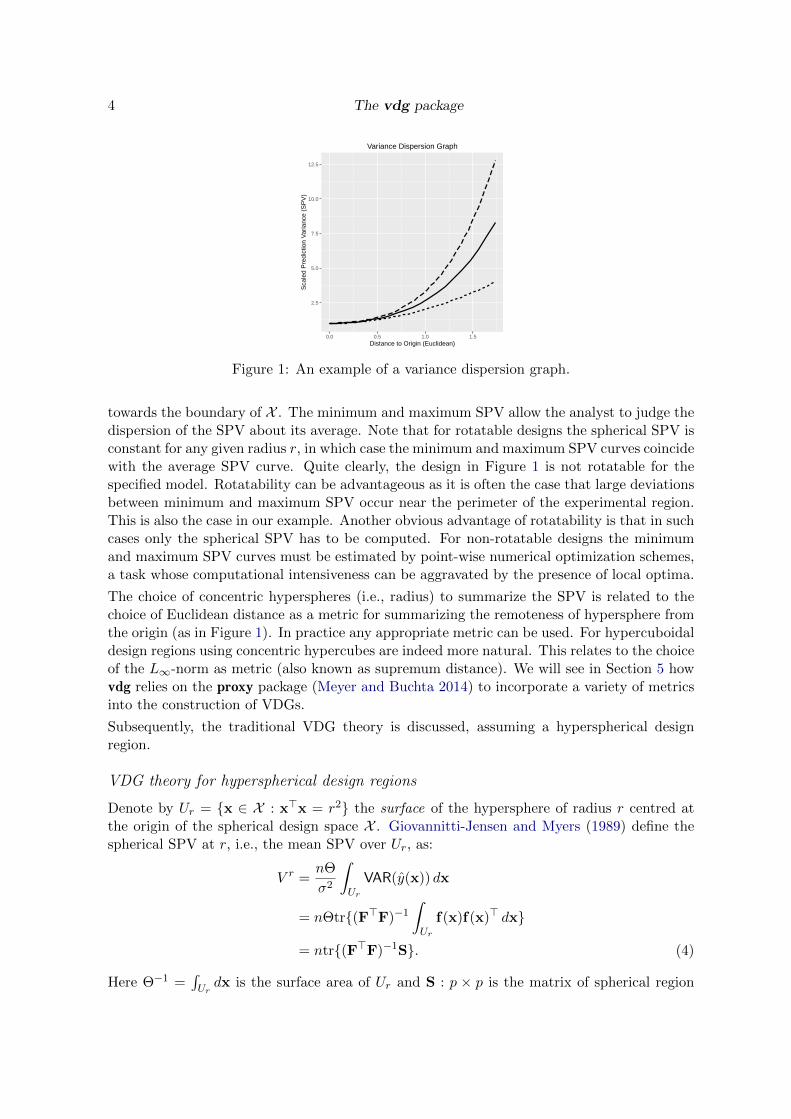
The VDG of Giovannitti-Jensen and Myers (1989) displays a summary of the SPV of thedesign ξn over the design region X . In the original formulation, the summary is achievedby concentric hyperspheres spanning X and usually centred at the origin. The VDG thensummarizes the SPV distribution by plotting the estimated minimum, average and maximumSPV on the surface of each hypersphere against the radius of the hypersphere. In this waythe high-dimensional SPV profile can always be summarized in a two-dimensional plot of theSPV values against the radius. An example is given in Figure 1, where X is spherical withmaximum radius

√3. Here the solid line represents the mean SPV, and the long and short

dashed lines the maximum and minimum SPV respectively. The mean of the SPV distributionover the surface of a hypersphere is also known as the spherical SPV.

Loading required package: parallel

Loading required package: ggplot2

Loading required package: quantreg

Loading required package: SparseM

Attaching package: ’SparseM’

The following object is masked from ’package:base’:

backsolve

Due to the uncertainty regarding where in the design space a prediction will be required,a stable SPV profile is desirable. A stable SPV is associated with a relatively flat VDGand cases where the maximum and minimum SPV curves do not deviate markedly from theaverage SPV. This is not the case for the design in Figure 1, where the SPV increases greatly

4 The vdg package

2.5

5.0

7.5

10.0

12.5

0.0 0.5 1.0 1.5Distance to Origin (Euclidean)

Sca

led

Pre

dict

ion

Var

ianc

e (S

PV

)

Variance Dispersion Graph

Figure 1: An example of a variance dispersion graph.

towards the boundary of X . The minimum and maximum SPV allow the analyst to judge thedispersion of the SPV about its average. Note that for rotatable designs the spherical SPV isconstant for any given radius r, in which case the minimum and maximum SPV curves coincidewith the average SPV curve. Quite clearly, the design in Figure 1 is not rotatable for thespecified model. Rotatability can be advantageous as it is often the case that large deviationsbetween minimum and maximum SPV occur near the perimeter of the experimental region.This is also the case in our example. Another obvious advantage of rotatability is that in suchcases only the spherical SPV has to be computed. For non-rotatable designs the minimumand maximum SPV curves must be estimated by point-wise numerical optimization schemes,a task whose computational intensiveness can be aggravated by the presence of local optima.

The choice of concentric hyperspheres (i.e., radius) to summarize the SPV is related to thechoice of Euclidean distance as a metric for summarizing the remoteness of hypersphere fromthe origin (as in Figure 1). In practice any appropriate metric can be used. For hypercuboidaldesign regions using concentric hypercubes are indeed more natural. This relates to the choiceof the L∞-norm as metric (also known as supremum distance). We will see in Section 5 howvdg relies on the proxy package (Meyer and Buchta 2014) to incorporate a variety of metricsinto the construction of VDGs.

Subsequently, the traditional VDG theory is discussed, assuming a hyperspherical designregion.

VDG theory for hyperspherical design regions

Denote by Ur = {x ∈ X : x>x = r2} the surface of the hypersphere of radius r centred atthe origin of the spherical design space X . Giovannitti-Jensen and Myers (1989) define thespherical SPV at r, i.e., the mean SPV over Ur, as:

V r =nΘ

σ2

∫Ur

VAR(y(x)) dx

= nΘtr{(F>F)−1∫Ur

f(x)f(x)> dx}

= ntr{(F>F)−1S}. (4)

Here Θ−1 =∫Urdx is the surface area of Ur and S : p × p is the matrix of spherical region

Pieter Schoonees, Niel le Roux, Roelof Coetzer 5

moments for Ur. Specifically, the elements of S have the form (Giovannitti-Jensen and Myers1989):

σ(δ) = Θ

∫Ur

xδ11 xδ22 . . . xδmm dx, (5)

where δ = (δ1, . . . , δm)>.

Due to the symmetry of the surface Ur, σ(δ) is zero whenever any of the {δi} are odd.Depending on the model, this property often leads to S being quite sparse. Often only a fewelements of δ are nonzero, and since the symmetry implies that it does not matter whichelements these are, it is notationally more convenient to characterize the spherical regionmoments in Equation 5 in terms of the values of the nonzero elements. As an example, thetwo-variable first-order model y = β0 +β1x1 +β2x2 + ε has a spherical region moment matrixof the form (Giovannitti-Jensen and Myers 1989): 1 0 0

0 σ2 00 0 σ2

(6)

where

σ2 =r2

m. (7)

For the model linear in the parameters, explicit equations for the spherical SPV function (aswell as for the minimum and maximum SPV curves) exist (see Giovannitti-Jensen and Myers1989). Note also that the second-order model in addition requires the following sphericalregion moments:

σ4 =3r4

m(m+ 2)(8)

σ22 =r4

m(m+ 2). (9)

In this case the form of S is more involved (for further details, see Giovannitti-Jensen andMyers 1989).

Generalizing to more flexible models

However, to consider more general models, or models containing only specific terms, moregeneral spherical region moments are required. For this purpose the VDG theory can beextended as follows. The formula for a general spherical region moment with all elements ofδ even is:

σ (δ) =

r1>δΓ

(m2

) m∏i=1

Γ(δi+12

)π

m2 Γ(1>δ+m

2

) . (10)

This formula can be derived from the evaluation of Equation 5 after using a transformationto polar coordinates (see for example Muirhead 1982, pp. 55-56) together with the propertiesof beta integrals. Considering the result in Equation 10, it is apparent that the spherical

6 The vdg package

moments are functions of the radius r and the number of design variables m only. Thehigher-order moments dominate the average SPV at large radii since the factor r1

>δ in theformula is monotonically increasing. Equation 10 has been implemented in vdg to calculatethe mean spherical SPV for any model formula (albeit subject to some restrictions – see?meanspv for details).

Advantages of the random sampling approach to VDGs

Note that although Equation 10 facilitates the analytical calculation of the average sphericalSPV curve, the minimum and maximum SPV must still be found by pointwise numericaloptimization techniques (except for first-order models – see Giovannitti-Jensen and Myers1989). This can be a tedious exercise as typically optimization needs to be done over a gridof radii spanning the design region X , and local optima may be problematic. The Fortranprogram of Vining (1993a,b) uses a combination of grid search and the Nelder-Mead simplexmethod, which can have erratic behaviour.

Although R provides a wide variety of other optimization possibilities – see for example theOptimization Task View on CRAN (Theussl 2014) – using the random sampling approachto explore X with the computational power available holds many advantages. In fact weargue that there is no need to use the exact minimum or maximum to assess the spread ofthe SPV. Instead of using pointwise optimization, vdg can use quantile regression throughmany randomly sampled points to give the user an impression of how e.g., the 5th and 95thpercentiles evolve for different radii. For this we use the excellent quantreg package (Koenker2013). At the same time the spread of the SPV at the randomly sampled points still gives anindication of the minimum or maximum SPV.

The form of the design region X is another important aspect to consider in the calculation ofVDGs. If X is non-spherical, for example cuboidal, Equation 10 does not hold for larger radiir for which only part of the hypersphere is contained in X . In such a case only the part ofthe concentric hyperspheres contained in X should contribute to the minimum, average andmaximum SPV curves, and truncation will be necessary. The ease with which the samplingapproach can allow for these and other nonstandard design regions is an important advantageover the optimization approach.

Furthermore, it is important to note that the maximum and minimum SPV values plotted onthe VDG only give an indication of the range of the spherical SPV. It is quite possible that twodesigns could have similar VDGs but quite different SPV distributions over the hyperspheres.In such a case, additional knowledge of the spherical SPV distribution is required, which isreadily available when using the random sampling approach. A traditional approach of thisflavour is the QPs described in the next Section.

2.2. Quantile plots

Related to the VDG is the QP of Khuri et al. (1996). QPs are based on the same principle asVDGs, but present more information about the distribution of the SPV over the hyperspheres.These plots use the quantiles of the SPV over the hyperspheres to display more informationand can therefore be used to distinguish between designs with similar VDGs but with differentSPV distributions.

In its original formulation, the basic idea of the QP is to graph the empirical cumulativedistribution functions (or ecdfs) of the SPV over each hypersphere for a number of concentric

Pieter Schoonees, Niel le Roux, Roelof Coetzer 7

2.5

5.0

7.5

10.0

12.5

0.00 0.25 0.50 0.75 1.00Proportion

SP

V Q

uant

ile

Radius

0.346

0.693

1.039

1.386

1.732

Figure 2: An example of a quantile plot, corresponding to the example in Figure 1.

hyperspheres with radii spanning the design region. These are estimated by randomly sam-pling a large number of points, say n∗, on the surface of each hypersphere. At each sampledpoint i the SPV dri is calculated and the ecdf of {dri } is computed. The QP then consists ofall the ecdf’s. If the sampled points adequately cover the experimental region, the resultinggraphs give detailed information about the distribution of the SPV over the experimentalregion. An example of such a QP is shown in Figure 2, where the quantiles of the SPV isplotted on the vertical axis. The lines in the plot represent the ecdf’s for five concentrichyperspheres, which is a more refined way of representing the information in Figure 1.

An alternative version of the QP displays boxplots side by side to summarize the SPV distri-bution at different radii. This leads to a display similar to the corresponding VDG. In vdgwe typically combine the information on display in a VDG and QP in a single graph (or aseries of related graphs).

2.3. Fraction of design space plots

The FDS plot, introduced by Zahran et al. (2003), is based on the argument that accurateprediction over the entire X must take into account the fraction of the volume of X thatis associated with the various values of the SPV. In contrast, the VDG and QP give equalweight to the SPV for all radii r, although the fraction of the volume of the design regionrepresented by the hypersphere of each radius differs substantially. This means that a smallSPV at a radius close to the origin does not give as much assurance of good prediction as asimilar SPV value at a larger radius.

The FDS plot is a way of correcting for this weighting problem which can make the use ofthe VDG and/or QP in isolation problematic. For example, it might occur that one design isfar superior (in terms of the SPV) compared to another for a small to moderate r, but onlysomewhat inferior at large r. From the VDG it will be tempting to choose the first designsince it is superior for most radii, but for higher dimensional design problems the designperformance at the boundaries of the design region becomes exponentially more important.Therefore the second design may be preferable.

FDS theory

For a fixed value ν of the SPV d(x, ξn), the FDS criterion is defined as

FDS (ν; ξn) = Φ−1∫Adx, (11)

8 The vdg package

2.5

5.0

7.5

10.0

12.5

0.00 0.25 0.50 0.75 1.00Fraction of Design Space

Sca

led

Pre

dict

ion

Var

ianc

e (S

PV

)

Fraction of Design Space Plot

Figure 3: An example of and FDS plot, corresponding to Figures 1 and 2.

where A = {x ∈ X : d (x, ξn) < ν} and Φ is the volume of X . The criterion therefore expressesthe volume of the set A containing all points in X with SPV lower than ν as a proportion ofthe total design space volume.

For each specified SPV value ν, the FDS plot graphs ν against FDS(ν). This in essenceamounts to calculating the cumulative distribution function (cdf) for the SPV values andrepresenting it graphically, albeit with a reversal of the usual horizontal and vertical axes(Goldfarb, Anderson-Cook, Borror, and Montgomery 2004). The latter reversal is motivatedby the need to make the FDS plots directly comparable to VDGs.

Since calculating the FDS criterion analytically becomes cumbersome in higher dimensions,an ecdf is used in practice to estimate the cdf described above. This is done through MonteCarlo simulation. First, a large number of points, say n∗, throughout X is generated. Foreach of these points the SPV is computed and finally the ecdf is calculated. A design wherethe SPV values are relatively small and does not vary much over the design region is desirable.

Figure 3 is an example of an FDS plot for the running example in Figures 1 and 2. We seethat for this design and model, the SPV is below 5 for 60% of the design region. The SPVexceeds 7.5 for roughly 12.5% of X , with less that 5% of X having an SPV value in excess of10.

Variants of FDS plots

Several variations of FDS plots exist. One variation is to use the so-called unscaled predictionvariance (or UPV) instead of the SPV of Equation 3. The UPV d∗(x, ξn) is defined as

d∗(x, ξn) = n · d(x, ξn) = σ−2 VAR(y(x)). (12)

The UPV is appropriate when the size and the related cost of two or more designs are notconsidered to be important. This can occur when the cost of individual runs are insignificant.

Another version of FDS plots is the scaled FDS plot which focuses on the stability of theprediction variance over the design region X (Zahran 2002). Here the normal FDS plot isadjusted by using the scaled SPV, which can be expressed as

d(x, ξn)

minx∈X d(x, ξn). (13)

Pieter Schoonees, Niel le Roux, Roelof Coetzer 9

A design with a steeper scaled SPV curve compared to another has a SPV which is less stableover the design region. This version of the FDS plot also allows the analyst to read off theratio of the maximum to the minimum SPV.

One further variant is the variance ratio FDS plot (or VRFDS, Rodriguez, Jones, Borror, andMontgomery 2010). This plot is especially useful when a number of candidate designs arebeing compared to a reference design. To construct such a plot, the SPV is calculated fora number of different designs at the same randomly simulated points over the design regionX . The VRFDS plot is then constructed by replacing the SPV with the natural logarithmof the ratio of the SPV of each design to the SPV of the reference design. Supposing thattwo designs, ξ1n1

and ξ2n2are of interest, the VRFDS plot is constructed by calculating the log

variance ratio

log V R(x∗, ξ1n1

; ξ2n2

)= log

d(x∗, ξ1n1

)d(x∗, ξ2n2

) (14)

for each simulated point x∗.

In Equation 14, ξ2n2is the reference design and is represented by a constant log variance ratio

of zero in the plot. If the log variance ratio for a design is negative, it has a lower SPV thanthe reference design and is therefore the preferred design. Similarly, when the log varianceratio is positive it has a larger SPV than the reference design and is therefore not preferred.A design which leads to better predictions over much of the experimental region will have acurve largely below the horizontal line representing the reference design. These VRFDS plotscan be useful for eliminating designs which are not admissible in the sense that they performworse compared to any other candidate design over most of the experimental region.

3. Simulation algorithms and guidelines

In this section the sampling algorithms used in the vdg package are introduced for exploringthe design space X . In addition, recommendations are provided regarding the number ofsamples required.

3.1. Simulation algorithms

It is important to note that random sampling of X has advantages compared to using a grid ofpoints covering the design region. Borkowski (2003) shows that using a grid of points placestoo much emphasis on the boundary regions of X , which leads to inaccurate SPV estimatessince the SPV is likely to be large at the perimeter of X . Although similar accuracy can beachieved for a fine grid of points, the relative efficiency remains lower.

In the design literature generally cuboidal or spherical design regions are commonly employed.Therefore these two cases will receive special attention here. Note however that using randomsampling to explore the design space implies that any type of design region can be consideredas long as it is possible to sample uniformly over it.

Sampling in hypercubes

A trivial way to generate uniform samples in an m-dimensional hypercube is to generateeach of the m coordinates independently as uniform random numbers. For X = [−a, a]m,

10 The vdg package

−1.0 −0.5 0.0 0.5 1.0

−1.

0−

0.5

0.0

0.5

1.0

X1

X2

Figure 4: An example of an LHS of 10 points in a two-dimensional design space.

the m-dimensional hypercube with sides of length 2a, each coordinate is simply generatedindependently as uniform variates on [−a, a].

Space-filling designs originate from the literature on computer experiments and provide analternative to this method (Fang, Li, and Sudjianto 2006). Simulation studies for FDS graphshave shown that Latin hypercube sampling (LHS) can be more efficient for large designproblems (Schoonees 2011). LHS was first introduced by McKay, Beckman, and Conover(1979). A Latin hypercube design is a design where each column of the n ×m matrix V isa random permutation of the column levels 1, 2, . . . , n. This matrix is then transformed intothe n×m design matrix X, by adding a random uniform value to each column. LHS amountsto first dividing X into a grid of equal sized hypercuboidal blocks. Then exactly one blockis selected from every dimension. Finally, a random uniform value is added to each selectedblock. An example of a LHS is given in Figure 4 and can be constructed as follows:

R> library("vdg")

R> set.seed(8745)

R> samp <- LHS(n = 10, m = 2, lim = c(-1, 1))

R> plot(samp, main = "", pty = "s", pch = 16, ylim = c(-1, 1),

+ asp = 1, xlab = expression(X[1]), ylab = expression(X[2]))

R> abline(h = seq(-1, 1, length.out = 10),

+ v = seq(-1, 1, length.out = 10), lty = 3, col = "grey")

Latin hypercube sampling thus provides an alternative to the grid procedure and the simpleuniform random sampling outlined previously. It can be seen as an extension to stratifiedsampling as it ensures that every portion of the range of each design factor is represented.Fang et al. (2006) show that LHS produces samples with a smaller variance of the samplemean than simple random sampling. The interested reader should consult their book for adetailed discussion of the subject.

Algorithm 1 provides an overview of the method. Four different variants are implemented invdg – see ?LHS and the examples for more details. It is also possible to interface to otherspace-filling design implementations, such as those available in for example lhs (Carnell 2012)and DiceDesign (Franco, Dupuy, Roustant, Damblin, and Iooss 2014). An example is givenin ?sampler.

Pieter Schoonees, Niel le Roux, Roelof Coetzer 11

Algorithm 1 Latin hypercube sampling algorithm on [−a, a]m (after Fang et al. 2006)

� Calculate b = [−a+ in ], i = 1, 2, . . . , n.

� For j = 1→ m:

– Permute the elements of b to give vj .

– Sample a vector of random numbers uj .

– Calculate xj as vj − 2an · uj .

� Form the matrix of samples as X =(x1 x2 · · · xm

).

Sampling in hyperspheres

The obvious method for obtaining a uniform random sample inside a hypersphere is therejection method – sample uniformly from the smallest hypercube containing the hypersphereand reject all samples falling outside the hypersphere. For higher dimensions and large samplesthis method is however inefficient. It is easy to show that the proportion of the volume ofa hypercube, contained in the largest hypersphere, rapidly approaches zero as the numberof dimensions m increases. It is therefore of interest to use alternative methods to generateuniform random samples within hyperspheres.

This can conveniently be achieved in two independent steps. The first requires a uniform sam-ple on the surface of the hypersphere with unit radius, after which each point is shrunken orextendend to the interior of the hypersphere by sampling radii from a particular distribution.The theory of spherical distributions, which includes the (multivariate) normal distribution,can be used to show that a point on the surface of the unit hypersphere can be found by sam-pling from a spherical distribution and rescaling the resulting vector to unit length (Schoonees2011; Muirhead 1982). This is readily achieved by concatenating m univariate samples frome.g., the normal distribution (rnorm() in R) and rescaling.

Furthermore, it can be shown that in order to ensure uniformity over the hypersphere, thecdf of the radius r on [0, R] is given by:

F (r) =Γ(m/2 + 1)

mπm/2Rm2(m−1)(m−2)/2+1rm

m−2∏i=1

B(m− i

2,m− i

2) (15)

where B(·, ·) denotes the Beta function. The inverse cdf method is used in vdg to sample therequired radii.

3.2. Simulation size

Ozol-Godfrey (2004) recommends using at least 10,000 randomly sampled points for an FDSgraph of up to eight factors. In practice, it is not harmful in terms of computation time to usemore. It should be clear from the plots produced by vdg whether or not a sufficient numberof samples had been used.

12 The vdg package

4. The vdg package

The design of vdg revolves around the spv() function, which creates objects of S3 classesspv, spvlist, spvforlist and spvlistforlist. These classes differ with respect to thenumber of designs and model formulae passed to them. For example, an object of classspvlistforlist results from a call where both arguments design and formula are lists ofdesigns and formulae repectively.

Objects of these classes contain the SPV (or unscaled prediction variance if unscaled =

TRUE) evaluated for all designs and formulae at a set of n points sampled throughout X . TheSPV is calculated by a simple Fortran subroutine, and parallelization over multiple designs orformulae are facilitated by the built-in parallel package.

The sample can be passed explicitly by the user via the sample argument, but usually isconstructed automatically by the sampler() function. The latter is a simple wrapper forthe sampling algorithms built into the package (see Section 3), and automatically handlesspherical and cuboidal design regions (via argument type). The user can request samplingon the surface of concentric hyperspheres or hypercubes by setting at = TRUE in a call tospv(). In such cases accurate FDS plots cannot be constructed however and hence will notbe produced. Rejection sampling for nonstandard design regions can be achieved by passingan appropriate function as the keepfun argument to spv(). In such cases sampling willcontinue until a sample of at least the requested size is obtained.

Besides simple print() methods, the power of vdg lies in its plot() methods, which produce avariety of graphs returned as a list of ggplot2 objects. Use is made of facets to produce differentpanels for different designs and/or formulae. These graphical objects can subsequently bemanipulated further, notably by using the theme functions in ggplot2. Which plots areproduced depend on the input class as well as a variety of arguments (including which =

1:5). Only the most important can be mentioned here.

The alpha parameter determines the transparency of the plotted points, which helps to builda picture of the density of the prediction variance. It is often worth fine tuning this parameter,although a default is provided. The vector tau of values between zero and one determineswhich quantile regressions are included in the VDGs. A nonnull value for the radii argumentimplies that the mean spherical prediction variance will be added to the VDGs according toEquation 10. It is advisable to read the help page of meanspv() when using this facility –there are limits to what types of formulas can be handled safely.

Finally, the optional method argument is passed to proxy::dist() and determines how thedistance between a sampled point and the origin of X is determined. Several metrics are avail-able, as described in summary(pr_DB) in proxy. If unset, the type argument will determinean appropriate value, namely Euclidean and supremum distance for spherical and cuboidaldesign regions respectively.

A starting point for exploring the package is ?’vdg-package’. The call

R> vignette(topic = "vdg", package = "vdg")

will display a version of this paper which also serves as package vignette.

5. Examples

Pieter Schoonees, Niel le Roux, Roelof Coetzer 13

D416B D416C

8

12

16

20

24

0.0 0.5 1.0 1.5 2.0 0.0 0.5 1.0 1.5 2.0Distance to Origin (Euclidean)

Sca

led

Pre

dict

ion

Var

ianc

e (S

PV

)

Location

Mean

tau = 0.05

tau = 0.95

Variance Dispersion Graph

Figure 5: A VDG for Roquemore’s hybrid designs D416B and D416C for a full quadraticmodel.

5.1. Comparing four-factor hybrid designs

As a first example, we compare Roquemore’s (Roquemore 1976) near-saturated 16-run hybriddesigns D416B and D416C for a full second-order model in four factors. These designs areavailable in Vdgraph as

R> library("Vdgraph")

R> data("D416B")

R> data("D416C")

We can construct a VDG for these designs with vdg simply by

R> quad4 <- formula( ~ (x1 + x2 + x3 + x4)^2 + I(x1^2) + I(x2^2) +

+ I(x3^2) + I(x4^2))

R> set.seed(1234)

R> spv1 <- spv(n = 5000, design = list(D416B = D416B,

+ D416C = D416C), formula = quad4)

R> plot(spv1, which = "vdgboth")

Of course quad4 could also have been specified more compactly as

R> quad4 <- formula( ~ .^2 + I(x1^2) + I(x2^2) + I(x3^2) + I(x4^2))

Figure 5 shows the resulting VDG for these two designs, where the 5th and 95th percentilesare shown as quantile regression fits, together with the mean spherical SPV. The individualsampled points are overplotted, which gives an indication of the distribution of the SPV overthe design region. It is evident that the SPV profiles for the hyperspherical design region Xare very similar for both designs. D416B has a slightly higher SPV in proximity of the origin,but performs better near the perimeter of the design space. Hence it can be expected that

14 The vdg package

8

12

16

20

24

0.00 0.25 0.50 0.75 1.00Fraction of Design Space

Sca

led

Pre

dict

ion

Var

ianc

e (S

PV

)

Design

D416B

D416C

Fraction of Design Space Plot

−0.05

0.00

0.05

0.10

0.00 0.25 0.50 0.75 1.00Fraction of Design Space

log(

SP

Vx

SP

Vre

f)

Design

D416B

D416C

Variance Ratio FDS Plot

Figure 6: A standard and variance ratio FDS plot for Roquemore’s hybrid designs D416Band D416C for a full quadratic model.

D416B is preferable to D416C for this model and design space. This is confirmed by the FDSplots constructed by

R> plot(spv1, which = "fds")

R> plot(spv1, which = "fds", VRFDS = TRUE, np = 100)

as shown in Figure 6. The right panel shows that D416B is slightly superior over the majorityof the design region.

Additional options to the which argument are outlined in ?plot.spv. Multiple plots can beproduced in a single call by passing a vector to which. Note that the plots are by defaultreturned as a list of ggplot2 graphical objects (see e.g., Murrell 2011). The plots are renderedwhen they are print()ed, which implies that on some graphics devices only the last plotwill be visible. This can be dealt with by either storing the resulting list of graphical objectsand rendering them one by one, or by specifying arrange = TRUE in the plot() call. Thelatter will arrange all plots in a single device by using grid.arrange() from the gridExtrapackage (Auguie 2012). Yet another option is to set par(ask = TRUE) before creating theplots, which will prompt the user before advancing to the next plot.

An advantage of storing the plots as graphical objects is that we can make post-hoc changesbefore rendering the plot. For example, we might not like the default ggplot2 theme used forFigure 5. We can easily change the theme to something more traditional with

R> p <- plot(spv1, which = "vdgboth")

R> p$vdgboth + theme_bw() + theme(panel.grid = element_blank())

The result is shown in Figure 7. Much more refined approaches are also possible; see forexample ?ggplot2::theme and Wickham (2009).

5.2. Central composite, D- and A-optimal designs

In this example we consider optimal design alternatives to central composite designs (CCDs)for three design factors. A hyperspherical design region is assumed, and the axial distance for

Pieter Schoonees, Niel le Roux, Roelof Coetzer 15

D416B D416C

8

12

16

20

24

0.0 0.5 1.0 1.5 2.0 0.0 0.5 1.0 1.5 2.0Distance to Origin (Euclidean)

Sca

led

Pre

dict

ion

Var

ianc

e (S

PV

)

LocationMean

tau = 0.05

tau = 0.95

Variance Dispersion Graph

Figure 7: A second version of Figure 5.

the CCD is assumed to be α =√

3. This spherical CCD is based on a full factorial design,augmented with four center runs and the usual six axial runs. The CCD hence contains 22runs, and we can construct it using rsm (Lenth 2009) as

R> library("rsm")

R> ccd3 <- as.data.frame(ccd(basis = 3, n0 = 4,

+ alpha = "spherical", oneblock = TRUE))[, 3:5]

We also construct a D- and A-optimal design with optFederov() from AlgDesign (Wheeler2014). For this purpose a candidate list of 10 000 randomly sampled points is constructedwithin the sphere of radius α, with runif_sphere() in vdg:

R> set.seed(8619)

R> cand <- runif_sphere(n = 10000, m = 3)

R> colnames(cand) <- colnames(ccd3)

The algorithm then attempts to select the 22 runs from these candidates which optimizethe requested criterion. D-optimality seeks to maximize the determinant of the informationmatrix in Equation 1, which implies minimizing the volume of the confidence ellipsoid of theregression parameters. A-optimality seeks to minimize the trace of the inverse informationmatrix, which minimizes the average variance of the regression parameters (for more details,see for example Myers et al. 2009). The D- and A-optimal designs can be found by executing

R> quad3 <- formula( ~ (x1 + x2 + x3)^2 + I(x1^2) + I(x2^2) + I(x3^2))

R> library("AlgDesign")

R> set.seed(3476)

R> desD <- optFederov(quad3, data = cand, nTrials = 22, criterion = "D")

R> desA <- optFederov(quad3, data = cand, nTrials = 22, criterion = "A")

All the information needed for the plots is obtained by calling spv() as

16 The vdg package

A CCD D

4

8

12

0.0 0.5 1.0 1.5 0.0 0.5 1.0 1.5 0.0 0.5 1.0 1.5Distance to Origin (Euclidean)

Sca

led

Pre

dict

ion

Var

ianc

e (S

PV

)

Variance Dispersion Graph

(a)

5

10

15

0.0 0.5 1.0 1.5Distance to Origin (Euclidean)

Sca

led

Pre

dict

ion

Var

ianc

e (S

PV

)

Location

Mean

tau = 0.05

tau = 0.95

Design

A

CCD

D

Variance Dispersion Graph

(b)

Figure 8: A FDS plot and VDG for the CCD, D- and A-optimal designs, for a full quadraticmodel in three factors on a spherical design region.

R> spv2 <- spv(n = 10000, formula = quad3,

+ design = list(CCD = ccd3, D = desD$design, A = desA$design))

R> plot(spv2, which = 2:3)

The VDG and FDS plots are shown in Figure 8. From the VDG it is apparent that the CCDand A-optimal designs have similar SPV profiles over X , where the SPV is very low nearthe origin but becomes increasingly worse towards the perimeter. The D-optimal design doesworse in the interior but at the same time have better SPV near the perimeter of X .

The FDS plot shows that the D-optimal design has the most stable SPV. Although the CCDand A-optimal designs achieve lower SPV values near the origin, this comes at the cost of asignificantly higher SPV near the perimeter of X . The FDS plot places more emphasis on theperimeter since this is where the majority of the volume of X is located. Hence the D-optimaldesign provides an alternative to the CCD which features better prediction over the majorityof the design region.

5.3. Cubic model with restricted design region

Chapter 5 of Goos and Jones (2011) describes an experimental problem in two variables,namely time (seconds) and temperature (degrees Kelvin), for a chemical reaction in an in-dustrial setting. The aim was to refine the current operating conditions to optimize the yieldof the chemical process. However, based on prior knowledge the experimental region X has arestricted shape, as shown in Figure 9. Outside this region the combination of design factorswas deemed not worth exploring by researchers with intimate knowledge of the process.

Furthermore, a full cubic model was decided on since a quadratic model was deemed inad-equate to capture the nonlinearity of the response process. A 15-run design was feasible –the D-optimal design employed by Goos and Jones (2011, Table 5.4) and shown in Figure 9is included in vdg as GJ54 (not all design points lie strictly within X ). In order to constructa VDG and FDS plot for this design, we need to be able to sample from X . Translating tostandardized coordinates on [−1, 1] in both time and termperature (using e.g., stdrange()

Pieter Schoonees, Niel le Roux, Roelof Coetzer 17

520

530

540

550

400 500 600 700Time

Tem

pera

ture

Figure 9: The design region and D-optimal design of Goos and Jones (2011). Some runs arereplicated.

in vdg), the equations of the linear restrictions on X are:

y = −1.08x+ 0.28

y = −0.36x− 0.76.

We can use this to construct a function keepfun() which takes a data matrix x and returnsa logical vector indicating which of the samples in the rows of x lie within X :

R> keepfun <- function(x) apply(x >= -1 & x <= 1, 1, all) &

+ (x[, 2] <= -1.08 * x[, 1] + 0.28) & (x[, 2] >= -0.36 * x[, 1] - 0.76)

We compare the SPV for the full cubic model, for which the design was constructed, tothis model without the cubic term for Time and the interaction between Temperature andthe quadratic term in Time. This latter model was the final model after removing the twoinsignificant effects – see Goos and Jones (2011). The formula for this model is obtained as

R> cube2 <- formula( ~ (Time + Temperature)^2 + I(Time^2) +

+ I(Temperature^2) + I(Time^3) + I(Temperature^3) +

+ Time:I(Temperature^2) + I(Time^2):Temperature)

R> GJmod <- update(cube2, ~ . - I(Time^3) - I(Time^2):Temperature)

To sample uniformly over X , we can use keepfun() to construct an spv object for the stan-dardized design. The algorithm will automatically keep sampling until at least the specifiednumber of samples have been obtained. We now pass a list of model formulae to spv(), anduse Latin hypercube sampling for illustration:

R> spv3 <- spv(n = 10000, design = stdrange(GJ54), type = "lhs",

+ formula = list(Cubic = cube2, GoosJones = GJmod),

+ keepfun = keepfun)

18 The vdg package

6

9

12

0.00 0.25 0.50 0.75 1.00Fraction of Design Space

Sca

led

Pre

dict

ion

Var

ianc

e (S

PV

)

Formula

Cubic

GoosJones

Fraction of Design Space Plot

Figure 10: VDG for the D-optimal design of Goos and Jones (2011), for the two models.

Retained samples: 5016 -- Adding some more...

Retained samples: 9976 -- Adding some more...

Final sample of size 10490

R> plot(spv3, which = 1, points.size = 2)

Of course the SPV surface for the second model is much favoured to the full cubic model,but the unimportance of the dropped terms is difficult if not impossible to establish beforeconstructing a design. Note in Figure 10 that supremum distance is automatically selectedto summarize the SPV since the argument type = "cuboidal" was specified. This can bechanged to e.g., Manhattan distance by passing method = "Manhattan" to the call to plot().Users are encouraged to experiment with the option hexbin = TRUE which uses ggplot2’shexagonal binning feature as an alternative to overplotting.

Since this example has only two variables, the SPV surface can also be inspected by contourplots, or in three dimensions by e.g., rgl (plot not shown; Adler, Murdoch, and others 2014):

R> library("rgl")

R> with(spv3$Cubic, plot3d(x = sample[, "Time"],

+ y = sample[, "Temperature"], z = spv))

6. Conclusions

The vdg package provides a modern and flexible R interface to important graphical proceduresin experimental design, producing VDGs, FDS and related plots using random sampling.Multiple designs and/or multiple model formulae are seamlessly allowed for, while using R’sformula interface allows for flexibility in model specification. Plots are produced with theggplot2 package, which allows for post hoc manipulation of graphical elements.

The flexibility of vdg empowers users to investigate irregular design regions; to use differentsampling schemes; to consider complicated model specifications; to construct different variantsof the standard plots, such as the VRFDS plot, as well as to enhance plots with novelties likequantile regressions. In addition to its capabilities illustrated in the examples given above,the plot method of vdg includes features like specifying specific distance measures from the

Pieter Schoonees, Niel le Roux, Roelof Coetzer 19

proxy package via the method argument and using hexagonal binning via hexbin = TRUE

instead of overplotting. Thus, vdg not only plays a complimentary role to the collection ofexisting R packages available to the practitioner in the field of experimental designs, but addsworthwhile capabilities for use in this field.

References

Adler D, Murdoch D, others (2014). rgl: 3D Visualization Device System (OpenGL). R pack-age version 0.93.1098, URL http://CRAN.R-project.org/package=rgl.

Atkinson AC, Donev AN, Tobias R (2007). Optimum Experimental Designs, with SAS. OxfordUniversity Press.

Auguie B (2012). gridExtra: Functions in Grid Graphics. R package version 0.9.1, URLhttp://CRAN.R-project.org/package=gridExtra.

Borkowski JJ (2003). “A Comparison of Prediction Variance Criteria for Response SurfaceDesigns.” Journal of Quality Technology, 35(1), 70–77.

Carnell R (2012). lhs: Latin Hypercube Samples. R package version 0.10, URL http://CRAN.

R-project.org/package=lhs.

Chaloner K, Verdinelli I (1995). “Bayesian Experimental Design: A Review.” StatisticalScience, 10(3), 273–304.

Fang KT, Li R, Sudjianto A (2006). Design and Modeling for Computer Experiments. Chap-man & Hall/CRC.

Franco J, Dupuy D, Roustant O, Damblin G, Iooss B (2014). DiceDesign: Designs of Com-puter Experiments. R package version 1.6, URL http://CRAN.R-project.org/package=

DiceDesign.

Giovannitti-Jensen A, Myers RH (1989). “Graphical Assessment of the Prediction Capabilityof Response Surface Designs.” Technometrics, 31(2), 159–171.

Goldfarb HB, Anderson-Cook CM, Borror CM, Montgomery DC (2004). “Fraction of De-sign Space Plots for Assessing Mixture and Mixture-Process Designs.” Journal of QualityTechnology, 36(2), 169–179.

Goos P, Jones B (2011). Optimal Design of Experiments: A Case Study Approach. JohnWiley & Sons.

Khuri AI, Kim HJ, Um Y (1996). “Quantile Plots of the Prediction Variance for ResponseSurface Designs.” Computational Statistics & Data Analysis, 22(4), 395–407.

Koenker R (2013). quantreg: Quantile Regression. R package version 5.05, URL http:

//CRAN.R-project.org/package=quantreg.

Lawson J (2013). The Vdgraph Package. R package version 2.1-3, URL http://CRAN.

R-project.org/package=Vdgraph.

20 The vdg package

Lenth RV (2009). “Response-Surface Methods in R, Using rsm.” Journal of Statistical Soft-ware, 32(7), 1–17. URL http://www.jstatsoft.org/v32/i07/.

McKay MD, Beckman RJ, Conover WJ (1979). “A Comparison of Three Methods for SelectingValues of Input Variables in the Analysis of Output from a Computer Code.” Technometrics,42(1), 239–245.

Meyer D, Buchta C (2014). proxy: Distance and Similarity Measures. R package version 0.4-12, URL http://CRAN.R-project.org/package=proxy.

Muirhead RJ (1982). Aspects of Multivariate Statistical Theory. John Wiley & Sons.

Murrell P (2011). R Graphics. 2nd edition. Chapman & Hall/CRC.

Myers RH, Montgomery DC, Anderson-Cook CM (2009). Response Surface Methodology:Process and Product Optimization Using Designed Experiments. John Wiley & Sons.

Ozol-Godfrey A (2004). Understanding Scaled Prediction Variance Using Graphical Methodsfor Model Robustness, Measurement Error and Generalized Linear Models for ResponseSurface Designs. Ph.D. thesis, Virginia Polytechnic Institute and State University.

R Core Team (2016). R: A Language and Environment for Statistical Computing. R Founda-tion for Statistical Computing, Vienna, Austria. URL http://www.R-project.org/.

Rodriguez M, Jones B, Borror CM, Montgomery DC (2010). “Generating and Assessing ExactG-Optimal Designs.” Journal of Quality Technology, 42(1), 3–20.

Roquemore KG (1976). “Hybrid Designs for Quadratic Response Surfaces.” Technometrics,18(4), 419–423.

Schoonees P, le Roux N, Coetzer R (2016). “Flexible Graphical Assessment of ExperimentalDesigns in R: The vdg Package.” Journal of Statistical Software, 74(3), 1–22. doi:10.

18637/jss.v074.i03.

Schoonees PC (2011). Sequential Experimental Design Strategies for Second-Order Models.Master’s thesis, University of Stellenbosch, South Africa.

Schoonees PC (2016). vdg: Variance Dispersion Graphs and Fraction of Design Space Plots.R package version 1.2.0, URL http://CRAN.R-project.org/package=vdg.

Srisuradetchai P, Borkowski JJ (2014). VdgRsm: Variance Dispersion and Fraction ofDesign Space Plots. R package version 1.01, URL http://CRAN.R-project.org/package=

VdgRsm.

Theussl S (2014). “CRAN Task View: Optimization and Mathematical Programming.” Ver-sion 2014-08-08, URL http://CRAN.R-project.org/view=Optimization.

Vining GG (1993a). “A Computer Program for Generating Variance Dispersion Graphs.”Journal of Quality Technology, 25(1), 45–58.

Vining GG (1993b). “Corrigenda to“A Computer Program for Generating Variance DispersionGraph”.” Journal of Quality Technology, 25(1), 333–335.

Pieter Schoonees, Niel le Roux, Roelof Coetzer 21

Wheeler B (2014). AlgDesign: Algorithmic Experimental Design. R package version 1.1-7.2,URL http://CRAN.R-project.org/package=AlgDesign.

Wickham H (2009). ggplot2: Elegant Graphics for Data Analysis. Springer-Verlag. ISBN978-0-387-98140-6. URL https://github.com/hadley/ggplot2-book.

Zahran AR (2002). On the Efficiency of Designs for Linear Models in Non-Regular Regionsand the Use of Standard Designs for Generalized Linear Models. Ph.D. thesis, VirginiaPolytechnic Institute and State University.

Zahran AR, Anderson-Cook CM, Myers RH (2003). “Fraction of Design Space to AssessPrediction Capability of Response Surface Designs.” Journal of Quality Technology, 35(4),377–386.

Affiliation:

Pieter C. SchooneesDepartment of Marketing ManagementRotterdam School of Management, Erasmus University3062PA Rotterdam, The NetherlandsE-mail: schoonees@rsm.nlURL: http://www.rsm.nl/

Niel J. le RouxDepartment of Statistics and Actuarial ScienceUniversity of StellenboschStellenbosch, South AfricaE-mail: njlr@sun.ac.zaURL: http://academic.sun.ac.za/statistics

Roelof L.J. CoetzerGroup Technology, Sasol South AfricaSasolburg, South AfricaE-mail: roelof.coetzer@sasol.com