flexible learning approach to physics ÊÊÊ module m6.3 ... … · flap m6.3 solving second-order...

F L E X I B L E L E A R N I N G A P P R O A C H T O P H Y S I C S

FLAP M6.3 Solving second-order differential equationsCOPYRIGHT © 1998 THE OPEN UNIVERSITY S570 V1.1

Module M6.3 Solving second order differential equations1 Opening items

1.1 Module introduction

1.2 Fast track questions

1.3 Ready to study?

2 Methods of solution for various second-order differential equations

2.1 Classifying second-order differential equations

2.2 Equations of the form d2y/dt2 = f(t); direct integration

2.3 The equation for simple harmonic motion:

d2y/dt2 + ω2y = 0

2.4 Equations of the form d2y/dt2 − λ2y = 0

2.5 The equation for damped harmonic motion: a(d2y/dt2) + b(dy/dt) + cy = 0

2.6 Equations of the forma(d2y/dt2) + b(dy/dt) + cy = f(t)

2.7 A worked example:damped, driven harmonic motion

3 Closing items

3.1 Module summary

3.2 Achievements

3.3 Exit test

Exit module


1 Opening items

1.1 Module introductionSuppose that we are interested in the behaviour of a mass m, free to bob up and down along the y-axis on the endof a spring of force constant k, and also subject to a damping (or resistive) force the magnitude of which isproportional to the speed of the mass, as well as to an externally imposed periodic force in the y-direction givenby Fy = F01sin1(Ω0t) where F0 is a positive constant. (Fy is commonly abbreviated to F to avoid unnecessaryconfusion with the subscripts.) The equation of motion of the mass is obtained by applying Newton’s secondlaw. If y is the displacement of the mass from equilibrium, then we have

md2 y

dt2= −ky − b

dy

dx+ F0 sin (Ωt) (1)


All the forces acting on the mass have been added together on the right-hand side of Equation 1,

md2 y

dt2= −ky − b

dy

dx+ F0 sin (Ωt) (Eqn 1)

and are as follows:

−ky (the restoring force exerted by the spring);

−bdy

dt, where b is a positive constant (the damping force);

F01sin1(Ω0t) (the periodic applied force).

Equation 1 is an example of a second-order linear differential equation. It belongs to a category of lineardifferential equations known as linear equations with constant coefficients, where the dependent variable and itsderivatives are multiplied by constants (not by functions of the independent variable).


The most general second-order equation of this sort can be written as

ad2 y

dt2+ b

dy

dt+ cy = f (t ) (2)

where a, b, c are constants and a ≠ 0; it is equations of this type that will be discussed in this module.

The simplest of this type of equation is one for which b and c are zero, so that the equation becomes

ad2 y

dt2= f (t ) (3)

This can be solved by direct integration, as will be explained in Subsection 2.1. Another relatively simple casearises when we have zero on the right-hand side of Equation 2, instead of a function of t, so that

ad2 y

dt2+ b

dy

dt+ cy = 0 , where a, b, c are constants and a ≠ 0 (4)

Equations of this type (known as linear homogenous equations) have innumerable applications in physics; theyarise, for example, in the discussion of simple harmonic motion and the analysis of a.c. circuits. Much of thismodule (Subsections 2.2 to 2.5) is therefore devoted to finding solutions to various forms of Equation 4.


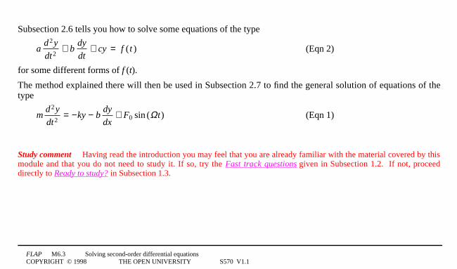
Subsection 2.6 tells you how to solve some equations of the type

ad2 y

dt2+ b

dy

dt+ cy = f (t ) (Eqn 2)

for some different forms of f1(t).

The method explained there will then be used in Subsection 2.7 to find the general solution of equations of thetype

md2 y

dt2= −ky − b

dy


Study comment Having read the introduction you may feel that you are already familiar with the material covered by thismodule and that you do not need to study it. If so, try the Fast track questions given in Subsection 1.2. If not, proceeddirectly to Ready to study? in Subsection 1.3.


1.2 Fast track questions

Study comment Can you answer the following Fast track questions?. If you answer the questions successfully you needonly glance through the module before looking at the Module summary (Subsection 3.1) and the Achievements listed inSubsection 3.2. If you are sure that you can meet each of these achievements, try the Exit test in Subsection 3.3. If you havedifficulty with only one or two of the questions you should follow the guidance given in the answers and read the relevantparts of the module. However, if you have difficulty with more than two of the Exit questions you are strongly advised tostudy the whole module.


Question F1

The angular displacement θ of the bob of a simple pendulum satisfies the equation of motion

ad

dtb

d

dtc

2

20

θ θ θ+ + =

(a) Find the general solution of this equation if a = 0.11kg, b = 0.21kg1s−1 and c = 1.01kg1s−2.(b) Find the particular solution if the bob is hit when in its rest position θ = 0 such that it is given an angular

speedd

dtt

θ = =−0 3 01. rad s at

(c) Sketch this solution as a function of t.

Question F2

Find the general solution to the equation

d2 x

dt2+ 5

dx

dt+ 6 x = 2 t 2

3


Study comment Having seen the Fast track questions you may feel that it would be wiser to follow the normal routethrough the module and to proceed directly to Ready to study? in Subsection 1.3.

Alternatively, you may still be sufficiently comfortable with the material covered by the module to proceed directly to theClosing items.


1.3 Ready to study?

Study comment In order to study this module you will need to be familiar with the following terms: degree(of a polynomial), exponential function, general solution, initial condition, linear differential equation andparticular solution. You will also need to be familiar with various trigonometric identities (although we will repeat themhere); to be able to solve first-order differential equations by direct integration (which requires a fair knowledge ofintegration methods); to know how to check a proposed solution to a differential equation by substitution (which requiresgood differentiation skills); and to be able to use initial conditions to obtain a particular solution from a general solution.To appreciate the physical significance of some of the equations appearing in this module, you should know how to useNewton’s second law to write down a differential equation describing the motion of an object if you are given informationabout the forces acting on it. Some familiarity with simple harmonic motion (SHM) would be particularly useful.If you are uncertain about any of these terms, you can review them now by reference to the Glossary, which will alsoindicate where in FLAP they are developed. The following Ready to study questions will allow you to establish whether youneed to review some of these topics before embarking on this module.


Question R1

Find the general solution to the differential equationdy

dx= x

1 + x2

Question R2

If y = 4ex/2 cos12x, calculate dy/dx and d12y/dx2.


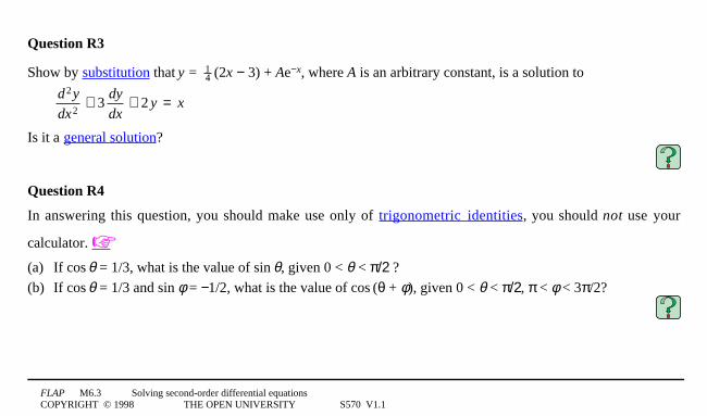
Question R3

Show by substitution that y = 14 (2x − 3) + Ae−x, where A is an arbitrary constant, is a solution to

d2 y

dx2+ 3

dy

dx+ 2 y = x

Is it a general solution?

Question R4

In answering this question, you should make use only of trigonometric identities, you should not use your

calculator.

(a) If cos1θ = 1/3, what is the value of sin1θ, given 0 < θ < π/2 ?(b) If cos1θ = 1/3 and sin1φ = −1/2, what is the value of cos1(θ + φ), given 0 < θ < π/2, π < φ < 3π/2?


Question R5

In each of the two following expressions for y, use the given initial conditions to calculate values for thearbitrary constants A and B.

(a) y = (At + B)e−21t; where y = 1 and dy/dt = 3 at t = 0.

(b) y = A1cos12x + B1sin12x; where y = 4 and dy/dx = −2 at x = 0.

Question R6

An object of mass m is free to move along a line; its displacement from the origin is denoted by x. It is acted onby three forces: a restoring force, the magnitude of which is proportional to the magnitude of x; a resistive(or damping) force, the magnitude of which is proportional to the cube of the object’s speed; and a constantforce of magnitude F0 acting in the negative x-direction. Use Newton’s second law to write down the second-order differential equation that x must satisfy.


2 Methods of solution for various second-order differential equations

Notation3Very often in the problems that arise in physics the independent variable is time, and so, whendiscussing a general type of differential equation, the independent variable is denoted by t and the dependentvariable by y. However, in some of the examples, drawn from specific problems in physics, we will use thenotation for the variables that is appropriate to the situation. Bear in mind that the quantity being differentiatedwill always be the dependent variable.


2.1 Classifying second-order differential equationsThere is such a wide variety of second-order differential equations that it is useful to divide them into variouscategories, and in this subsection we will introduce some terminology that arises when we do so. You areprobably already familiar with the distinction between linear and non-linear differential equations. The mostgeneral linear second-order differential equation is of the form

a(t )d2 y

dt2+ b(t )

dy

dt+ c(t )y = f (t )

where a(t), b(t), c(t) and f1(t) are functions of t.

However, in many of the second-order linear equations that you will encounter in your study of physics thedependent variable and its derivatives appear multiplied only by constants rather than functions of t.Such an equation is known as a linear differential equation with constant coefficients and has the form

ad2 y

dt2+ b

dy

dt+ cy = f (t ) (5)


Equation 5

ad2 y

dt2+ b

dy

dt+ cy = f (t ) (Eqn 5)

is easiest to solve when its right-hand side is zero, i.e. when

ad2 y

dt2+ b

dy

dt+ cy = 0 (6)

As you see, all the terms in Equation 6 contain the dependent variable y or a derivative of y; for that reason, anequation of this form is called a linear homogeneous differential equation. We will discuss equations of thissort in Subsections 2.3, 2.4 and 2.5. If f1(t) in Equation 5 is not zero, then the equation is called alinear inhomogeneous differential equation (as there is now a term in the equation which does not involve thedependent variable y). Equation 6 is relatively easy to solve, whereas the ease with which we are able to solveEquation 5 is crucially dependent on the form of the function f1(t).


Question T1

State whether the following differential equations are linear with constant coefficients and, if so, whether theyare homogeneous or inhomogeneous:

(a) d2 y

dx2= x − 3y

3

(b) xd2 y

dx2+ 2

dy

dx+ y = 0

3

(c) d2 x

dt2− 5

dx

dt= 6 x

3

We will first dispose of the easiest of all second-order differential equations1—1those that may be solved bydirect integration. This is the subject of the next subsection.


2.2 Equations of the form d2y/dt2 = f(t); direct integration

You should already know how to solve a first-order differential equation of the form

dy

dt= f (t ) (7)

where the derivative of the dependent variable is equal to a function of the independent variable. This equationmay be integrated directly, to give

y = f (t ) dt∫ (8)

The indefinite integral will involve one arbitrary constant of integration, this indicates that Equation 8 gives usthe general solution to Equation 7.


It is just as straightforward to solve a second-order differential equation of the form

d2 y

dt2= f (t ) (9)

where the second derivative of the dependent variable is equal to a function of the independent variable.Here, we simply integrate directly twice. Recalling that d12y/dt2 is the derivative of dy/dt, we see that if weintegrate both sides of Equation 9, we obtain

dy

dt= f (t ) dt = F(t ) + A∫ (10)

where F(t) is an indefinite integral of f1(t) (i.e. F(t) is a function such that F1′(t) = dF(t)/dt = f1(t)), and A is aconstant of integration. If we integrate Equation 10 again we obtain:

y = F(t ) + A( )∫ dt = G(t ) + At + B (11)

where G(t) is an indefinite integral of F(t), and B is another constant of integration. We see that Equation 11contains two arbitrary constants, A and B; this indicates that it is the general solution to Equation 9.


Equations which can be directly integrated often arise when considering objects that are moving along a line.For instance, an object moving along the x-axis, with position coordinate x and acceleration ax(t), a knownfunction of time, satisfies the equation

d x

dta tx

2

2= ( ) (12)

The following example illustrates this.


Example 1 A car is travelling in the x-direction along a straight road. At time t = 0, it starts to accelerate, andfor the next 81s, its acceleration ax(t) is given by ax(t) = a + bt. If a = 2.001m1s−2, b = 0.501m1s−3 and the car’svelocity is 5.001m1s−1 at t = 0, how far does the car travel during the 81s period?

Solution We must first solve the differential equation

d x

dta bt

2

2= +

where x = x(t) is the position of the car and we take the origin to be the position of the car at t = 0, so that x = 0at t = 0. Integrating once gives us

dx

dt= (a + bt)∫ dt = at + b

t2

2

+ A = at + b

2t2 + A

where A is an arbitrary constant. On substituting dx/dt = 5.001m1s−1 at t = 0 into this equation, we findA = 51m1s−1.


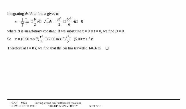
Integrating dx/dt to find x gives us

x atb

t A dtat bt

At B= + +

⌠⌡

= + +2 2 6

22 3

where B is an arbitrary constant. If we substitute x = 0 at t = 0, we find B = 0.

So xt t

t= + +− − −( . ) ( . ) ( . )0 506

2 002

5 0033

22

1m s m s m s

Therefore at t = 81s, we find that the car has travelled 146.61m.3


Sometimes, instead of being given information directly about the acceleration of the object, you may be giventhe force Fx(t) acting on it as a function of time. However, since Fx(t) = max(t), where m is the mass of theobject, it is very easy to write down a differential equation of the form given in Equation 12.

d x

dta tx

2

2= ( ) (Eqn 12)

Such a differential equation, arising from an application of Newton’s second law, is often called anequation of motion.

Try the following question, which illustrates another example.

Question T2

An object of mass 21kg, which is constrained to move along the x -axis, is subject to a force

Fx(t) = F01cos1(Ω1t), acting along the x-axis (in the direction of increasing x), where F0 = 41N and Ω = 21s−1.

At time t = 0, the object’s displacement is +31m and its velocity is +11m1s−1. Find its displacement as a functionof time.3


2.3 The equation for simple harmonic motion:d2y/dt2 + w12y = 0

We will now make a start at finding solutions of Equation 6,

ad2 y

dt2+ b

dy

dt+ cy = 0 (Eqn 6)

In this subsection (and the next), we will look at the simplified case where b = 0, so that Equation 6 takes theform

ad2 y

dt2+ cy = 0 (13)

In Equation 13, a ≠ 0 (so the equation is of second order) and c ≠ 0. (If c were zero, we could solve the equationby direct integration.) Since a ≠ 0, we can divide both sides of the equation by a, and write h = c/a to give:

d2 y

dt2+ hy = 0 (14)


d2 y

dt2+ hy = 0 (14)

You will see shortly that the form of solution of Equation 14 depends on whether the constant h is positive ornegative. We will consider these two possibilities separately, starting with the case of positive h.(The case of negative h will be discussed in Subsection 2.4.) If h is positive, we can make it clear that this is soby writingh = ω0

2, so that Equation 14 becomes:

d2 y

dt2+ ω0

2 y = 0 (SHM equation) (15)

Before discussing the solutions to Equation 15, we will emphasize the importance of this equation in physics.It is the equation of motion of any object undergoing simple harmonic motion (SHM)1—1motion where theforce acting on the object is proportional to the object’s displacement from some point and acts in the oppositedirection to the displacement. For this reason, Equation 15 is often known as the SHM equation.


You may already know that an object undergoing SHM executes oscillations and we will see shortly that theperiod of the oscillations depends on the parameter ω0 which is known as the angular frequency in the contextof Equation 15.

d2 y

dt2+ ω0

2 y = 0 (Eqn 15)

So it is important that whenever you encounter a case of SHM, you should be able to rewrite the differentialequation describing the physical situation in the form of Equation 15, and so find an expression for ω0 in termsof the parameters appearing in the problem. The following question gives you practice in this.


L

C

Figure 13See Question T3(a).

mO

θ

l

Figure 23See Question T3(b).

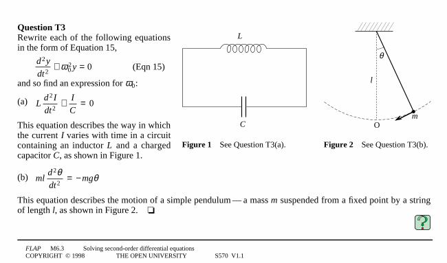
Question T3Rewrite each of the following equationsin the form of Equation 15,

d2 y

dt2+ ω0

2 y = 0 (Eqn 15)

and so find an expression for ω0:

(a) Ld2 I

dt2+ I

C= 03

This equation describes the way in whichthe current I varies with time in a circuitcontaining an inductor L and a chargedcapacitor C, as shown in Figure 1.

(b) mld2θdt2

= − mgθ3

This equation describes the motion of a simple pendulum1—1a mass m suspended from a fixed point by a stringof length l, as shown in Figure 2.3


It is not too difficult to guess the general solution of Equation 15.

d2 y

dt2+ ω0

2 y = 0 (Eqn 15)

Any solution of this equation must be a function such that when we differentiate it twice, we recover thefunction itself, multiplied by −ω102. This should remind you of a cosine or a sine function. In fact, both cos1(ω10t)and sin1(ω0t) have precisely this property, as does any function of the form B1cos1(ω0t) + C1sin1(ω0t), where B andC are arbitrary constants.

Show that y = B1cos1(ω0t) + C1sin1(ω0t) is a solution to Equation 15.

You have now shown that

the first form of the solution to the SHM equation (Equation 15) is:

y(t) = B1cos1(ω10t) + C1sin1(ω100t) (16)

Since it contains two arbitrary constants B and C, it is the general solution.


Question T4

Write down the general solution of the following equations:

(a) d y

dx

2

2 + 25y = 03(b) 9

2

2

d Q

dx = −14Q3

It is easy to see from Equation 16

y(t) = B1cos1(ω10t) + C1sin1(ω100t) (Eqn 16)

that y(t) is a periodic function of t1—1that is, a function that ‘repeats itself’ each time t increases by a fixedamount, known as the period of the function. As you know, the value of a sine or cosine function isunchanged if the argument of the function is increased by 2π, or an integer multiple of 2π. Thus y has the samevalue if t increases by an amount T = 2π/ω0.

The quantity T = 2

0

πω

is therefore the period of the function given in Equation 16.


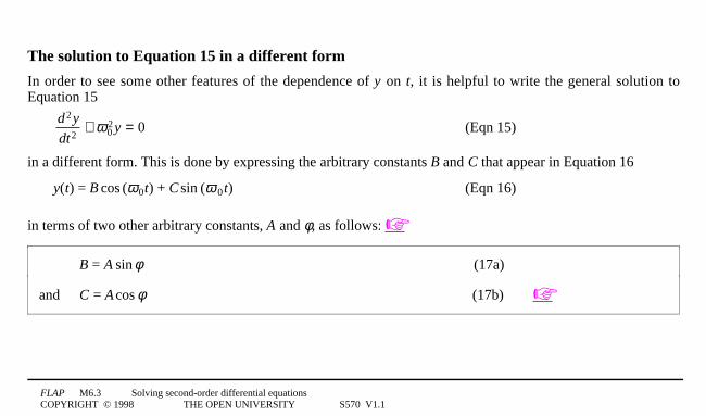
The solution to Equation 15 in a different form

In order to see some other features of the dependence of y on t, it is helpful to write the general solution toEquation 15

d2 y

dt2+ ω0

2 y = 0 (Eqn 15)

in a different form. This is done by expressing the arbitrary constants B and C that appear in Equation 16


in terms of two other arbitrary constants, A and φ, as follows:

B = A1sin1φ (17a)

and C = A1cos1φ (17b)


With these expressions for B and C, Equation 16


becomes

y = A1sin1φ 1cos1(ω0t) + A1cos1φ 1sin1(ω0t) = A[sin1φ 1cos1(ω0t) + cos1φ 1sin1(ω0t)] (18)

We may now use the trigonometric identity

sin1(α + β1) = sin1α 1cos1β + cos1α 1sin1β

to rewrite the right-hand side of Equation 18 and make it look a lot neater.


d2 y

dt2+ ω0

2 y = 0 (Eqn 15)

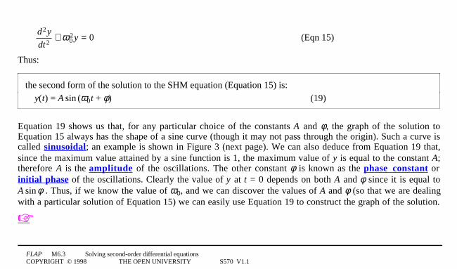
Thus:

the second form of the solution to the SHM equation (Equation 15) is:

y(t) = A1sin1(ω0t + φ) (19)

Equation 19 shows us that, for any particular choice of the constants A and φ, the graph of the solution toEquation 15 always has the shape of a sine curve (though it may not pass through the origin). Such a curve iscalled sinusoidal; an example is shown in Figure 3 (next page). We can also deduce from Equation 19 that,since the maximum value attained by a sine function is 1, the maximum value of y is equal to the constant A;therefore A is the amplitude of the oscillations. The other constant φ is known as the phase constant orinitial phase of the oscillations. Clearly the value of y at t = 0 depends on both A and φ since it is equal toA1sin1φ . Thus, if we know the value of ω0, and we can discover the values of A and φ (so that we are dealingwith a particular solution of Equation 15) we can easily use Equation 19 to construct the graph of the solution.


−2

2

0 π 2π

π12

−

y/m

t/s

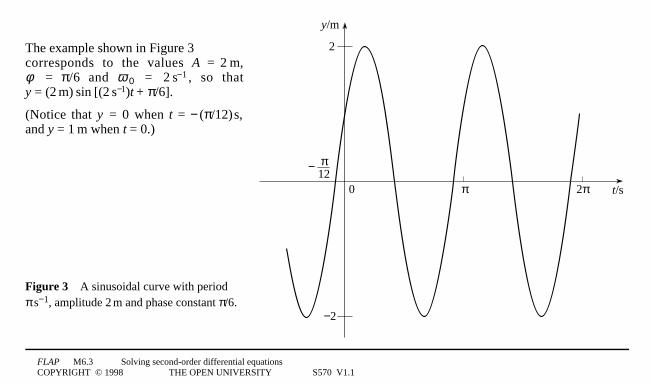
The example shown in Figure 3corresponds to the values A = 21m,φ = π/6 and ω0 = 21s−1 , so thaty = (21m)1sin1[(21s−1)t + π/6].

(Notice that y = 0 when t = − (π/12)1s,and y = 11m when t = 0.)

Figure 33A sinusoidal curve with periodπ1s−1, amplitude 21m and phase constant π/6.


Converting from one form of the solution into the other

It is clearly important to be able to switch between the two forms of the solution to the SHM equation given inEquations 16 and 19.


y(t) = A1sin1(ω0t + φ) (Eqn 19)

From Equations 17a and b we can easily calculate B and C if we are given values for A and φ; but how do wecalculate A and φ from known values of B and C? To see how to do this, note that if

B = A1sin1φ and C = A1cos1φ (Eqns 17a, b)

then

B2 + C12 = A2 (sin2φ +1cos12φ) = A2

so that

A2 = B2 + C12


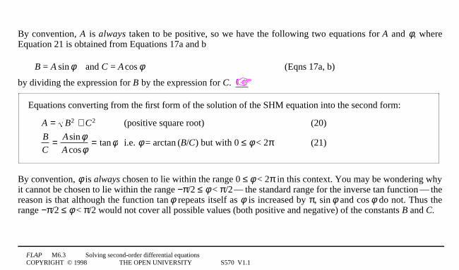
By convention, A is always taken to be positive, so we have the following two equations for A and φ, whereEquation 21 is obtained from Equations 17a and b


by dividing the expression for B by the expression for C.

Equations converting from the first form of the solution of the SHM equation into the second form:

A B C= +2 2 (positive square root) (20)

B

C

A

A= =sin

costan

φφ

φ i.e. φ = arctan1(B/C) but with 0 ≤ φ < 2π (21)

By convention, φ is always chosen to lie within the range 0 ≤ φ < 2π in this context. You may be wondering whyit cannot be chosen to lie within the range −π/2 ≤ φ < π/21—1the standard range for the inverse tan function1—1thereason is that although the function tan1φ repeats itself as φ is increased by π, sin1φ and cos1φ do not. Thus therange −π/2 ≤ φ < π/2 would not cover all possible values (both positive and negative) of the constants B and C.


In fact, using Equation 17,


and our knowledge of the properties of sin1φ and cos1φ, we can lay down some rules for the range of valueswithin which φ must lie, depending on whether B and C are positive or negative:

B ≥ 0 and C ≥ 0 ⇒ 0 ≤ φ ≤ π 2 (22a)

B ≥ 0 and C < 0 ⇒ π 2 < φ ≤ π (22b)

B < 0 and C < 0 ⇒ π < φ < 3π 2 (22c)

B < 0 and C ≥ 0 ⇒ 3π 2 ≤ φ < 2π (22d)

You can now use Equations 17, 20, 21 and 22

A B C= +2 2 (positive square root) (Eqn 20)

B

C

A

A= =sin

costan

φφ

φ i.e. φ = arctan1(B/C) but with 0 ≤ φ < 2π (Eqn 21)

to answer the following questions:


Question T5

Write the particular solution y = 61sin1(3t + π/3) in the form y = B1cos1(ω0t) + C1sin1(ω0t).3

Question T6

Write the two following particular solutions in the form y = A1sin1(ω0t + φ):

(a) y = 41cos1(2t) + 31sin1(2t)

(b) y = 51sin1(4t) − 121cos1(4t)3


2.4 Equations of the form d2y/dt2 - l2y = 0We will now return to the case of negative h in Equation 14.

d2 y

dt2+ hy = 0 (Eqn 14)

If h is negative, we can make it clear that this is so by writing h = −λ2, where (by convention) λ > 0, so thatEquation 14 becomes

d2 y

dt2− λ2 y = 0 (23)

You may not have yet encountered any physical situations that could be described by an equation of this sort.However, it does have important applications in quantum physics and elsewhere. So it is well worth your whileto learn how to solve this equation. Moreover, the solution is very easy to find.


To solve Equation 23,

d2 y

dt2− λ2 y = 0 (Eqn 23)

let us proceed using the same sort of informed guesswork that we used to solve Equation 15.

d2 y

dt2+ ω0

2 y = 0 (Eqn 15)

In the case of Equation 15, we wanted to find a function such that its second derivative was equal to the functionitself multiplied by a negative constant. Looking at Equation 23, we see that this time we want a function(or functions) the second derivative of which is equal to the function itself multiplied by a positive constant.Exponential functions have the property that all their derivatives are proportional to the function itself.

So let us see if an exponential function, of the form

y = Bept (24)

where B is an arbitrary constant, is a solution of Equation 23.


If we differentiate Equation 24 once,

y = Bept (Eqn 24)

we find dy/dt = pBe1pt = py.

When we differentiate again, we find

d2 y

dt2= p

dy

dt= p2 y

and on substituting this result into Equation 23,

d2 y

dt2− λ2 y = 0 (Eqn 23)

we obtain

p2y − λ2y = 0

which is an identity provided that p2 = λ2.

Thus Equation 24 is a solution to Equation 23 provided p = +λ or p = −λ.


It follows that any function of the form

y = Beλt (25a)

or y = Ce−λt (25b)

(We have replaced the arbitrary constant B in Equation 25a by the arbitrary constant C in Equation 25b.)

is a solution to Equation 23.

d2 y

dt2− λ2 y = 0 (Eqn 23)

Neither of these equations can themselves be the general solution of Equation 23, as neither contains twoarbitrary constants. But perhaps their sum, which does contain two arbitrary constants, is the general solution.

Show that y = Beλt + Ce−λt is a solution to Equation 23.


d2 y

dt2− λ2 y = 0 (Eqn 23)

So you have shown that:

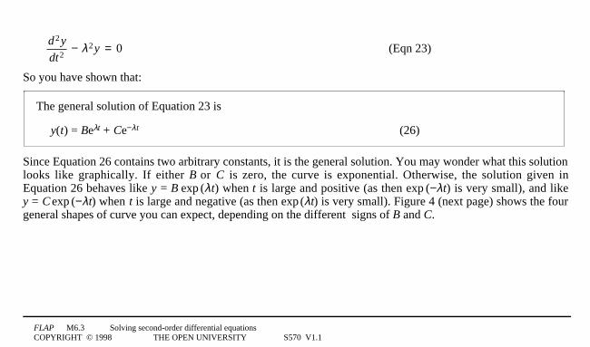
The general solution of Equation 23 is

y(t) = Beλt + Ce−λt (26)

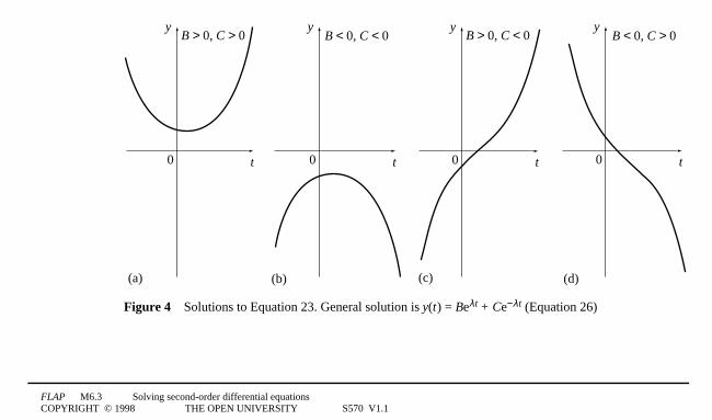
Since Equation 26 contains two arbitrary constants, it is the general solution. You may wonder what this solutionlooks like graphically. If either B or C is zero, the curve is exponential. Otherwise, the solution given inEquation 26 behaves like y = B 1exp1(λt) when t is large and positive (as then exp1(−λt) is very small), and likey = C1exp1(−λt) when t is large and negative (as then exp1(λt) is very small). Figure 4 (next page) shows the fourgeneral shapes of curve you can expect, depending on the different signs of B and C.


y

t0

y

t0

y

t0

y

t0

(a) (b) (c) (d)

B > 0, C > 0 B < 0, C < 0 B > 0, C < 0 B < 0, C > 0

Figure 43Solutions to Equation 23. General solution is y(t) = Beλt + Ce−λt (Equation 26)


Question T7

Find the general solution of

d2 y

dx2− 4 y = 0

and the particular solution if y = 6 and dy/dx = 0 at x = 0.3

We obtained the general solution given in Equation 26

y(t) = Beλt + Ce−λt (Eqn 26)

by taking the sum of the two solutions given in Equation 25.

y = Beλt (25a) or y = Ce−λt (Eqn 25b)

In fact, it can be proved that, for any linear homogeneous equation (not necessarily one with constantcoefficients) the sum of two solutions (or more than two, if the equation is of higher order than the second) isalways also a solution. We will not give the proof here (although the last marginal note should provide a hint asto how the proof might go), but you should bear this useful result in mind; we will make use of it in the nextsubsection.


2.5 The equation for damped harmonic motion:a(d2y/dt2) + b(dy/dt) + cy = 0

In Subsection 2.3, we mentioned that an equation of the form

ad2 y

dt2+ cy = 03where c/a = h > 0

has many different applications in physics, describing, as it does, the behaviour of an object undergoing simpleharmonic motion. Its solutions are sinusoidal oscillations of constant amplitude. However, you know fromexperience that the vibrations of an oscillating object always die away with time (pendulum clocks run down;masses bobbing up and down on springs come to rest, and so on). This is due to the effect of resistive ordamping forces, which oppose the motion of the oscillating object. How can we modify the SHM equation(Equation 15).

d2 y

dt2+ ω0

2 y = 0 (Eqn 15)

to take account of these forces? Let us return to the example mentioned in Subsection 1.1, a mass m oscillatingup and down on a spring of force constant k.


If the restoring force of the spring, −ky, is the only force acting on the mass, then, according to Newton’s secondlaw, its displacement y(t) must satisfy the equation

md2 y

dt2= −ky

To incorporate the effects of a damping force, we must add a term on the right-hand side which always acts in adirection opposite to the direction of the velocity of the mass (the bob). A simple way of doing this is to assumethat the damping force can be written in the form −b(dy/dt), where b is a positive constant, so that the equationof motion of the mass becomes

md2 y

dt2= −ky − b

dy

dt

i.e. md2 y

dt2+ b

dy

dt+ ky = 0 (27)


L

CR

Figure 53A circuit containing aninductance L, a resistor R and acapacitor C, connected in series.

An equation of the form given in Equation 27

md2 y

dt2+ b

dy

dt+ ky = 0 (Eqn 27)

also arises in the theory of a.c. circuits.

The current I in the circuit shown in Figure 5, containing an inductance L,a resistor R and a capacitor C, obeys the differential equation

Ld2 I

dt2+ R

dI

dt+ I

C= 0 (28)


To predict the behaviour of the mass on the spring, or the current in the circuit, you need to be able to solvedifferential equations of the type

ad2 y

dt2+ b

dy

dt+ cy = 03where a > 0, b > 0 and c > 0 (29)

We need the ratio b/a to be positive if the coefficient of dy/dt is to represent a resistive force, opposing thevelocity of the object; and we need the ratio c/a to be positive so that if b is zero, we recover the SHM equation(Equation 15).

d2 y

dt2+ ω0

2 y = 0 (Eqn 15)

This condition is most simply achieved by restricting all three constants to positive values. (In fact, the solutionswe obtain to Equation 29 will apply equally well if any of a, b, or c is negative.)


Let us now try to find solutions to Equation 29.

ad2 y

dt2+ b

dy

dt+ cy = 03where a > 0, b > 0 and c > 0 (Eqn 29)

We know that if b = 0, then the solution is a sinusoidal function. However, we do not want a purely sinusoidalsolution if b > 0 (we want y to tend to zero as t becomes large and positive, due to the damping); moreover, ifyou try a solution of the form y = sin1(1pt) or cos1(1pt) in Equation 29, you will quickly find that it does not work(unless b = 0, of course). But perhaps an exponential function would work, just as it did for Equation 23?

d2 y

dt2− λ2 y = 0 (Eqn 23)

We have nothing to lose by trying it, so let us substitute

y = Bept (30)

into Equation 29.


The first derivative of y is equal to py, and the second derivative is equal to p2y; so we find, on substitution,

ap2y + bpy + cy = 0

which is an identity provided that p satisfies the equation

ap2 + bp + c = 0 (auxilliary equation) (31)

This quadratic equation in p is known as the auxiliary equation of Equation 29.

ad2 y

dt2+ b

dy


As it is a quadratic, the roots of Equation 31 are given by

pb b ac

ap

b b ac

a1

2

2

242

42

= − + − = − − −and (32)

This formula will give us two real values for p1 and p2 provided that b2 > 4ac. (We will deal with the caseswhere b2 < 4ac or b2 = 4ac shortly; but for the moment, let us assume that the two roots are real.)


We have shown, therefore, that the trial solution, Equation 30,

y = Bept (Eqn 30)

will satisfy Equation 29

ad2 y

dt2+ b

dy


for any value of B provided that p is one of the two roots given in Equation 32.

pb b ac

ap

b b ac

a1

2

2

242

42

= − + − = − − −and (Eqn 32)


Real roots of the auxiliary equation (heavy damping)

We can write the two solutions of Equation 29

ad2 y

dt2+ b

dy


we have just found as

y = B1exp1(1p1t)3and3y = C1exp1(1p2t)

As we mentioned at the end of Subsection 2.4, we can obtain the general solution to Equation 29 by adding thesetwo solutions together:

The general solution of Equation 29 in the case b2 > 4ac is

y(t) = B1exp1(1p1t) + C1exp 1(1p2t) (33)

where3 pb b ac

a1

2 42

= − + −3and3 p

b b ac

a2

2 42

= − − −


or, written out in full,

y = B exp−b + b2 − 4ac

2at

+ C exp−b − b2 − 4ac

2at

(34)

There is no need to memorize this unpleasant-looking equation1—1but you should remember the method that weused to derive it, and be able to apply it to a given differential equation, as in the following example.

Example 2 Find the general solution of the differential equation

d2 y

dt2+ 5

dy

dt+ 6 y = 0

Solution First write down the auxiliary equation,

p2 + 5p + 6 = 0

This equation has two real roots:

p = − 52 ± 1

2 25 − 24 = −2 or − 33

Thus the general solution is y = Be−2t + Ce−3t .3


Question T8

Find the general solution of the differential equation

6d2 y

dt2+ 17

dy

dt+ 12 y = 03


t

y

0

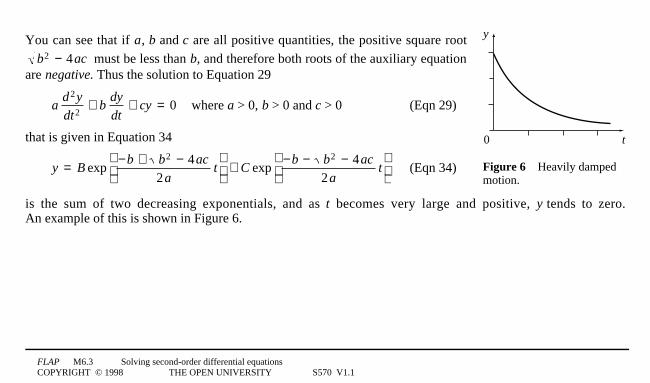
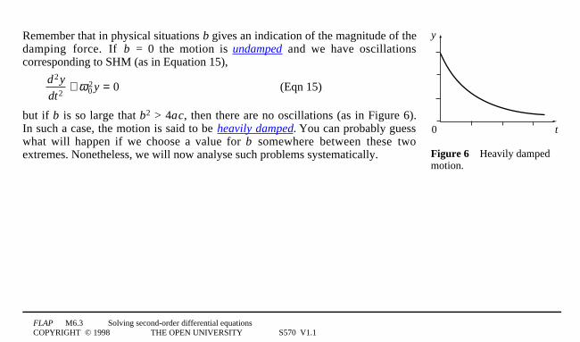
Figure 63Heavily dampedmotion.

You can see that if a, b and c are all positive quantities, the positive square root

b2 − 4ac must be less than b, and therefore both roots of the auxiliary equationare negative. Thus the solution to Equation 29

ad2 y

dt2+ b

dy


that is given in Equation 34

y = B exp−b + b2 − 4ac

2at

+ C exp−b − b2 − 4ac

2at

(Eqn 34)

is the sum of two decreasing exponentials, and as t becomes very large and positive, y tends to zero.An example of this is shown in Figure 6.


t

y

0

Figure 63Heavily dampedmotion.

Remember that in physical situations b gives an indication of the magnitude of thedamping force. If b = 0 the motion is undamped and we have oscillationscorresponding to SHM (as in Equation 15),

d2 y

dt2+ ω0

2 y = 0 (Eqn 15)

but if b is so large that b2 > 4ac, then there are no oscillations (as in Figure 6).In such a case, the motion is said to be heavily damped. You can probably guesswhat will happen if we choose a value for b somewhere between these twoextremes. Nonetheless, we will now analyse such problems systematically.


Complex roots of the auxiliary equation (light damping)

We will now solve Equation 29

ad2 y

dt2+ b

dy


for the case b2 < 4ac. We will give two alternative treatments of this important case.

The first treatment depends on a result that comes from the study of complex numbers, and shows that thesolution in this case is merely an extension of the previous result.

The second treatment does not require as much knowledge of complex numbers, we will just give you thesolution of the differential equation and ask you to verify that what we say is correct.


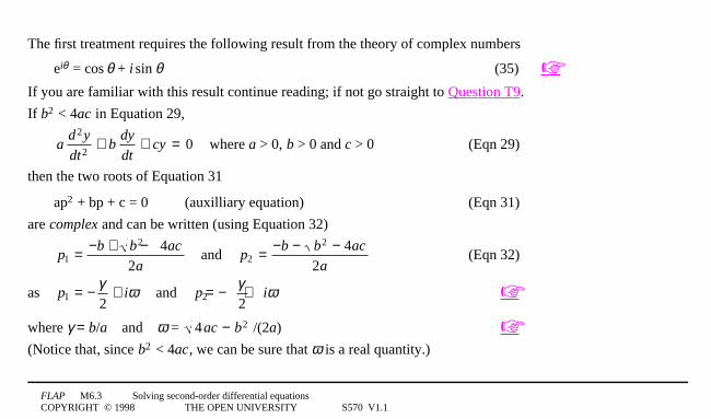
The first treatment requires the following result from the theory of complex numbers

eiθ = cos1θ + i1sin1θ (35) If you are familiar with this result continue reading; if not go straight to Question T9.

If b2 < 4ac in Equation 29,

ad2 y

dt2+ b

dy


then the two roots of Equation 31

ap2 + bp + c = 0 (auxilliary equation) (Eqn 31)

are complex and can be written (using Equation 32)

pb b ac

ap

b b ac

a1

2

2

242

42

= − + − = − − −and (Eqn 32)

as p i p i1 22 2

= − + = − +γ ω γ ωand

where γ = b/a3and3ω = 4ac − b2 /(2a)3 (Notice that, since b2 < 4ac, we can be sure that ω is a real quantity.)


Thus, the general solution to Equation 29

ad2 y

dt2+ b

dy


when b2 < 4ac is similar to that given in Equation 33

y(t) = B1exp1(1p1t) + C1exp 1(1p2t) (Eqn 33)

and we may write it as

y = R exp − γ2

+ iω

t

+ S exp − γ2

− iω

t

= exp(− γ t 2) R exp(iω t)[ ] + S exp(−iω t)[ ] (36)

where R and S are arbitrary constants.


It looks as though this solution will give complex values to y. However, since the case b2 < 4ac frequently arisesin physics problems, it must be possible to arrange Equation 36

y = R exp − γ2

+ iω

t

+ S exp − γ2

− iω

t

= exp(− γ t 2) R exp(iω t)[ ] + S exp(−iω t)[ ] (Eqn 36)

in a form which need not involve any complex quantities. We do this by employing Equation 35,

eiθ = cos1θ + i1sin1θ (Eqn 35)

to write

exp1(iω1t) = cos1(ω1t) + i1sin1(ω1t)3and3exp1(−iω1t) = cos1(ω1t) − i1sin1(ω1t)

if we substitute these results into Equation 36, we find

y = exp1(γ1t1/2)[(R + S)1cos1(ω1t) + i(R − S)1sin1(ω1t)]

We can now define new arbitrary constants B = R + S and C = i(R − S), and rewrite the solution as

y = exp1(−γ1t/2)[B1cos1(ω1t) + C1sin1(ω1t)]


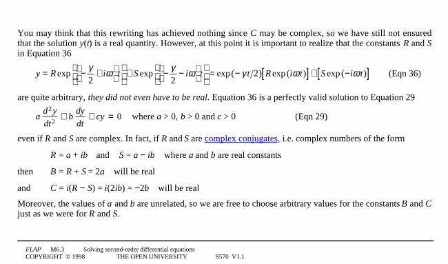
You may think that this rewriting has achieved nothing since C may be complex, so we have still not ensuredthat the solution y(t) is a real quantity. However, at this point it is important to realize that the constants R and Sin Equation 36

y = R exp − γ2

+ iω

t

+ S exp − γ2

− iω

t

= exp(− γ t 2) R exp(iω t)[ ] + S exp(−iω t)[ ] (Eqn 36)

are quite arbitrary, they did not even have to be real. Equation 36 is a perfectly valid solution to Equation 29

ad2 y

dt2+ b

dy


even if R and S are complex. In fact, if R and S are complex conjugates, i.e. complex numbers of the form

R = a + ib3and3S = a − ib3where a and b are real constants

then B = R + S = 2a3will be real

and C = i(R − S) = i(2ib) = −2b3will be real

Moreover, the values of a and b are unrelated, so we are free to choose arbitrary values for the constants B and Cjust as we were for R and S.


ad2 y

dt2+ b

dy


Thus:

The general solution of Equation 29 in the case b2 < 4ac is

y(t) = exp1(−γ1t1/2)[(B1cos1(ω1t) + C1sin1(ω1t)] (37)

with γ = b/a (38a)

and ω = 4ac − b2 /(2a) (38b)


Question T9

Show by substitution that, for arbitrary constants B and C,

y(t) = exp1(−γ1t1/2)[B1cos1(ω1t) + C1sin1(ω1t)]

where

γ = b/a3and3ω = 4ac − b2 /(2a)

is a solution to Equation 29.

ad2 y

dt2+ b

dy


(Notice that ω is a real quantity if b2 < 4ac.)3


The combination [B1cos1(ω1t) + C1sin1(ω1t)] appears in Equation 37,

y(t) = exp1(−γ1t1/2)[(B1cos1(ω1t) + C1sin1(ω1t)] (Eqn 37)

and it may be convenient to write this instead in the form A1sin1(ω1

t + φ), as we did in Subsection 2.3, by putting

A B C= +2 2 (Eqn 20)

and φ = arctan1(B/C)3but with 0 ≤ φ < 2π (Eqn 21)

This gives:

The alternative form of the solution of Equation 29 in the case b2 < 4ac

y(t) = A1exp1(−γ1t/2)1sin1(ω1

t + φ) (39)

with γ = b/23and3ω = 4ac − b2 /(2a) (Eqn 38a and b)

From Equation 39 it is easy to determine the behaviour of the function y(t). Since b/a is positive, γ is alsopositive1—1so y(t) is given by a sinusoidal function multiplied by an exponential function that decays as tbecomes large and positive.


0

y

t

2πω

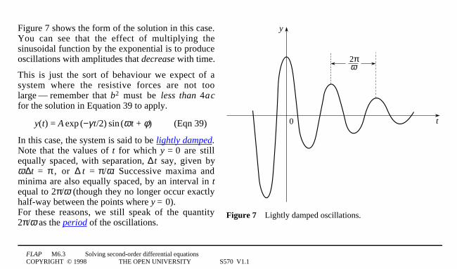
Figure 73Lightly damped oscillations.

Figure 7 shows the form of the solution in this case.You can see that the effect of multiplying thesinusoidal function by the exponential is to produceoscillations with amplitudes that decrease with time.

This is just the sort of behaviour we expect of asystem where the resistive forces are not toolarge1— 1remember that b2 must be less than 4acfor the solution in Equation 39 to apply.


t + φ) (Eqn 39)

In this case, the system is said to be lightly damped.Note that the values of t for which y = 0 are stillequally spaced, with separation, ∆ t say, given byω1

∆t = π, or ∆ t = π/ω. Successive maxima andminima are also equally spaced, by an interval in tequal to 2π/ω (though they no longer occur exactlyhalf-way between the points where y = 0). For these reasons, we still speak of the quantity2π/ω as the period of the oscillations.


Equal roots of the auxiliary equation (critical damping)

Finally, we will consider the case where b2 = 4ac which (although it is somewhat artificial in that it rarely occursin practice) is of interest because it marks the transition from light to heavy damping. In this case, the auxiliaryEquation 31


has only one root; from Equation 32,

pb b ac

ap

b b ac

a1

2

2

242

42

= − + − = − − −and (Eqn 32)

we see that p1 = p2 = −b/(2a). We deduce that y = B1exp1[−bt/(2a)] is a solution of the differential equationEquation 29.

ad2 y

dt2+ b

dy



However, it cannot be the general solution, since it only contains one arbitrary constant. The other solution thatwe must add to it is not at all obvious, so we will just tell you the answer, and leave you to check it bysubstitution.

ad2 y

dt2+ b

dy


It turns out

The general solution of Equation 29 in the case b2 = 4ac is

y(t) = (B + Ct)1exp1[−bt0/(2a)] (40)

Question T10

Show that Equation 40 is a general solution of Equation 29 in the case b2 = 4ac.3


This has been a long and quite complicated subsection, which is perhaps misleading since in practice thesolution of Equation 29 is fairly straightforward, and just a matter of knowing how to deal with three cases.Here then is a summary of the steps you need to follow in order to solve the equation of damped harmonicmotion:

ad2 y

dt2+ b

dy

dt+ cy = 0 (Eqn 29)

Step 1 Evaluate the quantity b2 − 4ac.

Step 2

o If b2 > 4ac, find the roots p1 and p2 of the auxiliary equation, Equation 31.


The general solution is then given by Equation 33.



o If b2 < 4ac, find the quantities γ and ω, using Equation 38.

with γ = b/a (Eqn 38a)

and ω = 4ac − b2 /(2a) (Eqn 38b)

The general solution is then given by Equation 37


(and then use Equations 20 and 21

A B C= +2 2 (Eqn 20)

and φ = arctan1(B/C)3but with 0 ≤ φ < 2π (Eqn 21)

if you want the solution in the form of Equation 39).


t + φ) (Eqn 39)

o If b2 = 4ac, the general solution is given by Equation 40.

y(t) = (B + Ct)1exp1[−bt0/(2a)] (Eqn 40)


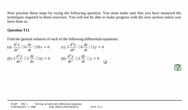
Now practise these steps by trying the following question. You must make sure that you have mastered thetechniques required in these exercises. You will not be able to make progress with the next section unless youhave done so.

Question T11

Find the general solution of each of the following differential equations:

(a) d2 x

dt2+ 6

dx

dt+ 10 x = 0 (c) 5

d2 y

dt2+ 6

dy

dt+ 2 y = 0

(b) 2d2 y

dx2+ 5

dy

dx+ 3y = 0 (d)

d2 y

dt2+ 2

dy

dt+ y = 0

3


The method of comparing b2 with 4ac and then selecting the form of the solution will of course work even ifb = 0, that is, for the differential equations discussed in Subsections 2.3 and 2.4. Consider, for example,

d2 y

dt2 + ω02 y = 0 (Eqn 15)

Here, b = 0, a = 1 and c = ω02. So b2 < 4ac, and Equation 38

γ = b/a (Eqn 38a)

ω = 4ac − b2 /(2a) (Eqn 38b)

tells us that γ = 0, ω = ω0. Thus using Equation 37,


we see that the general solution is y(t) = B 1cos1(ω0t) + C1sin1(ω0t), which is just what we found before, inEquation 16.



2.6 Equations of the form a(d2y/dt2) + b(dy/dt) + cy = f(t)We are now in a position to set about finding solutions to the general second-order linear inhomogeneousequation with constant coefficients:

ad2 y

dt2+ b

dy

dt+ cy = f (t ) (Eqn 5)

We will first of all show that if we can find any one particular solution to Equation 5, then we can always findthe general solution. We will then show a method that can sometimes be used to find particular solutions.


Let us suppose that we have somehow managed to find a particular solution to Equation 5;

ad2 y

dt2+ b

dy

dt+ cy = f (t ) (Eqn 5)

we will call it yp(t). We now assert that the general solution is obtained by taking the sum of yp(t) and thegeneral solution to the homogeneous equation which is obtained by setting f1(t) = 0 in Equation 5:

ad2 y

dt2+ b

dy

dt+ cy = 0 (41)

In this context, the general solution to the homogeneous equation (Equation 14)

d2 y

dt2+ hy = 0 (Eqn 14)

is called the complementary function; we will denote it by yc(t). Thus the claim here is that the general solutionto Equation 5 is

y(t) = yp(t) + yc(t) (42)


This result is easy to prove. We simply substitute Equation 42

y(t) = yp(t) + yc(t) (Eqn 42)

into Equation 5.

ad2 y

dt2+ b

dy

dt+ cy = f (t ) (Eqn 5)

The left-hand side becomes

ad2

dt2( yp + yc ) + b

d

dt( yp + yc ) + c( yp + yc )

which is equal to

ad2 yp

dt2+ b

dyp

dt+ cyp + a

d2 yc

dt2+ b

dyc

dt+ cyc (43)

but by assumption, yp is a solution to Equation 5; that is

ad2 yp

dt2+ b

dyp

dt+ cyp = f (t )


and yc is the general solution to Equation 41,

ad2 y

dt2+ b

dy

dt+ cy = 0 (Eqn 41)

so that

ad2 yc

dt2+ b

dyc

dt+ cyc = 0

So we see from Equation 43

ad2 yp

dt2+ b

dyp

dt+ cyp + a

d2 yc

dt2+ b

dyc

dt+ cyc (Eqn 43)

that, with the substitution y = yp + yc, the left-hand side of Equation 5

ad2 y

dt2+ b

dy

dt+ cy = f (t ) (Eqn 5)

is equal to f1(t) + 0, i.e. equal to f1(t). Thus Equation 42

y(t) = yp(t) + yc(t) (Eqn 42)

is a solution to Equation 5; it is the general solution since yc contains two arbitrary constants.


You should read through the following example carefully because it typifies the method which we apply to allsuch equations.

Example 3 Find the general solution to the differential equation

d y

dty t

2

24+ = (44)

Given that y = t/4 is a particular solution.


Solution To find the general solution, we must add the complementary function to the particular solution.The complementary function is the general solution of the homogeneous equation that we obtain by setting theright-hand side of Equation 44 to zero,

d y

dty t

2

24+ = (Eqn 44)

d2 y

dt2+ 4 y = 0

This equation is of the form given in Equation 15,

d2 y

dt2+ ω0

2 y = 0 (Eqn 15)

with ω0 = 2. Its general solution is given by Equation 16


to be B1cos1(2t) + C1sin1(2t). So the general solution to Equation 44

is y = t/4 + B1cos1(2t) + C1sin1(2t).3


Question T12Find the general solution to the differential equation

d2 y

dt2+ 3

dy

dt− 4 y = 2e−3t

given that y = − e−3t

2 is a particular solution.3


Finding a particular solution

So we now know how to find a general solution to a linear inhomogeneous equation if we are given a particularsolution. But how can we find a particular solution? There are several methods for doing this, and we willexplain here only the simplest. It is sometimes known as the method of undetermined coefficients, but as youwill see, it consists of little more than intelligent guesswork. The idea is that, guided by the form of f1(t), weshould assume a particular form for yp(t) which contains some undetermined constants, and simply substitutethis into the differential equation. If the form we have chosen is correct, we will be able to determine theconstants appearing in our trial solution from the requirement that we must obtain an identity on making thesubstitution. If we have not chosen the correct form, then we will find that it is not a solution, and we must thinkagain! The method can best be explained by an example.


Example 4 Find a particular solution to the differential equation

d2 y

dt2+ 4

dy

dt+ 5y = t + 2

Solution There is a function of the form Ht + K on the right-hand side of this equation. A function of this sort(a polynomial) has the property that when it is differentiated any number of times, no new functions of t appearin its derivatives1—indeed, the results are just constants (or zero). This suggests that the differential equationmight be satisfied by a function of this sort, with H and K suitably chosen. We may as well try it, anyway.If we put y = Ht + K into the equation, we obtain

4H + 5(Ht + K) = t + 2

i.e. 5Ht + (4H + 5K) = t + 2

This equation must be an identity if y = Ht + K is a solution. Thus the coefficients of t on both sides must be thesame, as must the constant terms. This gives us two equations to be solved for H and K:

5H = 13and34H + 5K = 2

These are easily solved, to give H = 1/5, K = 6/25. So we have found a particular solution; it isy = t/5 + 6/25.4


If we were to try to generalize the reasoning in Example 4, it would go something like this. The particularsolution must be such that when we substitute it into the left-hand side of the equation, f1(t) is recovered.If f1(t) is a function whose derivatives are all of the same form as f1(t) itself (such as a polynomial, an exponentialfunction or a sinusoidal function), we may be able to achieve this by trying as a particular solution a functionwhich is also of the form of f1(t), but contains some as yet unknown constants (the ‘undetermined coefficients’),the values of which we will determine when we make the substitution. This leads to the following rules forfinding particular solutions, for certain forms of f1(t):


Rules for finding particular solutions, for certain forms of f1(t):1 If f1(t) is a polynomial of degree m: try a particular solution that is also a polynomial of degree m

yp(t) = Ht0m + Ktm−1 + … + N

but containing undetermined coefficients H, K … N

2 If f1(t) is an exponential, Cekt: try a particular solution that is also an exponential,

yp(t) = Hekt

where H is an undetermined coefficient. 3 If f1(t) is a sinusoidal function, f1(t) = C1sin1(kt) + D1cos1(kt): try a particular solution that is also a sinusoidal

function

yp(t) = H1sin1(kt) + K1cos1(kt)

where H, K are undetermined coefficients.

You can now use Rules 1–3 to answer the following question.


Question T13

Find a particular solution to each of the following equations

(a)d2 y

dx2+ 2

dy

dx+ 3y = 2e− x

(b)d y

dx

dy

dxy x x

2

24 4 2 11+ + = −cos sin 3

The method of undetermined coefficients will work for some more complicated forms of f1(t), but we have saidenough here for you to be able to find particular solutions to many second-order inhomogeneous equations ofphysical interest. (It is worth pointing out, though, that if f1(t) is given by a sum of two or more functions of thesorts mentioned in Rules 1–3, then the particular solution is simply the sum of the particular solutionscorresponding to each of these functions.) At the end of the next subsection, in Question T14, you can puttogether the methods you have learnt so far to find general solutions to inhomogeneous equations.First, however, we will consider an example of great importance in physics.


2.7 A worked example: damped driven harmonic motion

We are now in a position to solve Equation 1, introduced in Subsection 1.1 ;

md2 y

dt2= −ky − b

dy


rewritten slightly, it is

md2 y

dt2+ b

dy

dt+ ky = F0 sin (Ω t) (45)

An equation of this sort applies whenever an oscillating object is subjected to a damping force −bdy

dt

as well as an external driving force, F01sin1(Ω1t) with angular frequency Ω. It is said to describe forced, damped oscillations or damped, driven oscillations.In this subsection, we will find the general solution to Equation 45 for the case b2 < 4mk.


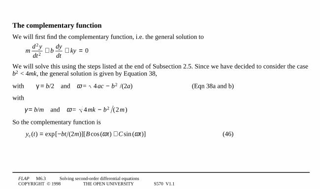
The complementary function

We will first find the complementary function, i.e. the general solution to

md2 y

dt2+ b

dy

dt+ ky = 0

We will solve this using the steps listed at the end of Subsection 2.5. Since we have decided to consider the caseb2 < 4mk, the general solution is given by Equation 38,

with γ = b/23and3ω = 4ac − b2 /(2a) (Eqn 38a and b)

with

γ = b/m3and3ω = 4mk − b2 (2m)

So the complementary function is

y t bt m B t C tc exp[( ) ( )][ cos( ) sin ( )]= − +2 ω ω (46)


A particular solution

We will now find a particular solution. We have a sinusoidal function on the right-hand side of Equation 45,

md2 y

dt2+ b

dy

dt+ ky = F0 sin (Ω t) (Eqn 45)

so, in accordance with Rule 3 at the end of Subsection 2.6, we will try a particular solution of the form

yp (t) = H cos(Ω t) + K sin (Ω t) .

On substituting this into Equation 45, we find

−mΩ2[H cos(Ωt) + K sin (Ωt)] + bΩ[−H (Ωt) + K cos(Ωt)] + k[H cos(Ωt) + K sin (Ωt)] = F0 sin (Ωt)


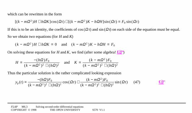
which can be rewritten in the form

[(k − mΩ 2 )H + bΩK ]cos(Ω t) + [(k − mΩ 2 )K − bΩH]sin (Ω t) = F0 sin (Ω t)

If this is to be an identity, the coefficients of cos1(Ω1t) and sin1(Ω1t) on each side of the equation must be equal.

So we obtain two equations (for H and K)

(k − mΩ 2 )H + bΩK = 03and3(k − mΩ 2 )K − bΩH = F0

On solving these equations for H and K, we find (after some algebra! )

H = −(bΩ )F0

(k − mΩ 2 )2 + (bΩ )23and3K = (k − mΩ 2 )F0

(k − mΩ 2 )2 + (bΩ )2

Thus the particular solution is the rather complicated looking expression

yp (t) = −(bΩ )F0

(k − mΩ 2 )2 + (bΩ )2cos(Ω t) + (k − mΩ 2 )F0

(k − mΩ 2 )2 + (bΩ )2sin (Ω t) (47)


We can simplify this greatly if we use Equations 20 and 21


B

C

A

A= =sin

costan

φφ


to write yp in the form

yp(t) = A1sin1(Ω1t + φ)

Applying Equations 20 and 21, we find (after some more algebra)

AF

k m b=

− +0

2 2 2( ) ( )Ω Ω(48a)

and φ = arctan−bΩ

k − mΩ 2

3but with 0 ≤ φ ≤ 2π (48b)


The general solution

Thus the general solution of Equation 45,

md2 y

dt2+ b

dy

dt+ ky = F0 sin (Ω t) (Eqn 45)

given by the sum of the complementary function (Equation 46)

y t bt m B t C tc exp[( ) ( )][ cos( ) sin ( )]= − +2 ω ω (Eqn 46)

and the particular solution (Equation 47),

yp (t) = −(bΩ )F0

(k − mΩ 2 )2 + (bΩ )2cos(Ω t) + (k − mΩ 2 )F0

(k − mΩ 2 )2 + (bΩ )2sin (Ω t) (Eqn 47)


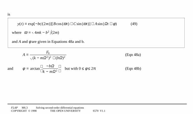
is

y(t) = exp[−bt (2m)][Bcos(ω t) + C sin (ω t)] + Asin (Ωt + φ ) (49)

where ω = −4 22mk b m( )

and A and φ are given in Equations 48a and b.

AF

k m b=

− +0

2 2 2( ) ( )Ω Ω(Eqn 48a)


k − mΩ 2

3but with 0 ≤ φ ≤ 2π (Eqn 48b)


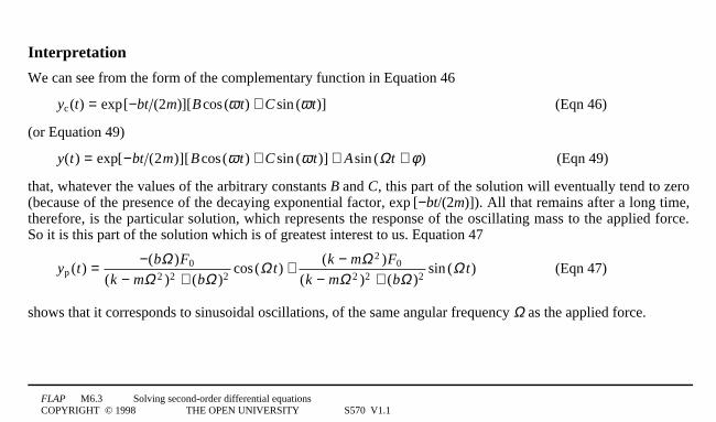
Interpretation

We can see from the form of the complementary function in Equation 46

y t bt m B t C tc exp[( ) ( )][ cos( ) sin ( )]= − +2 ω ω (Eqn 46)

(or Equation 49)

y(t) = exp[−bt (2m)][Bcos(ω t) + C sin (ω t)] + Asin (Ωt + φ ) (Eqn 49)

that, whatever the values of the arbitrary constants B and C, this part of the solution will eventually tend to zero(because of the presence of the decaying exponential factor, exp1[−bt/(2m)]). All that remains after a long time,therefore, is the particular solution, which represents the response of the oscillating mass to the applied force.So it is this part of the solution which is of greatest interest to us. Equation 47

yp (t) = −(bΩ )F0

(k − mΩ 2 )2 + (bΩ )2cos(Ω t) + (k − mΩ 2 )F0

(k − mΩ 2 )2 + (bΩ )2sin (Ω t) (Eqn 47)

shows that it corresponds to sinusoidal oscillations, of the same angular frequency Ω as the applied force.


However, there is a constant phase difference φ between the oscillations of the mass and oscillations of thedriving force. Mathematically, φ represents the amount by which the movement of the mass leads the force, butphysically it makes more sense to say that the motion lags behind the force by an amount 2π − φ.Notice (from Equations 48a and b)

AF

k m b=

− +0

2 2 2( ) ( )Ω Ω(Eqn 48a)


k − mΩ 2

3but with 0 ≤ φ ≤ 2π (Eqn 48b)

that the amplitude A of the oscillations depends not only on F0, but also on Ω; in other words, applied forces ofdifferent frequency may invoke oscillations of the mass of very different magnitude.


0.05

0.04

0.03

0.02

0.01

00 5 10 15 20 25 30 35

Ω/s−1

A/m

Figure 83Graph of A as a function of Ω, in the case m = 0.21kg,

b = 1.01N1s1m−1, k = 801N1m−1, F0 = 0.8 1N.

Figure 8 shows A as a function of Ω, for acertain choice of the parameters m, k, b and F0.You can see that it has a pronouncedmaximum at a value of Ω close to thenatural angular frequency ω0 = k m .

This large response for a particular value ofthe angular frequency of the applied force isthe well-known phenomenon of resonance.


The above example involved some rather unpleasant algebra (because we wished to discuss a general case),however, finding the general solution to a specific inhomogeneous equation is generally straightforwardenough1—1provided, of course, that f1(t) is one of the functions mentioned in Rules 1–3 at the end of Subsection2.61—1the method is summarized here:

1 Find the complementary function, using the methods of Subsection 2.5

2 Find the particular solution, using one of Rules 1–3 in Subsection 2.6

3 Add the two together.

You can practise these steps by trying the following question.

Question T14

Find the general solution to the equation

d2 y

dt2+ 6

dy

dt+ 9 y = 1 + 3t3


3 Closing items

3.1 Module summary1 A linear differential equation with constant coefficients has the form:

ad2 y

dt2+ b

dy

dt+ cy = f (t ) (Eqn 5)

If f1(t) in Equation 5 is set to zero it is a linear homogeneous differential equation. If f1(t) is not zero inEquation 5 it is a linear inhomogeneous differential equation

2 Equations of the form

d2 y

dt2 = f1(t) (Eqn 9)

can be solved by direct integration.


3 The general solution of the SHM (simple harmonic motion) equation

d2 y

dt2+ ω0

2 y = 0 (Eqn 15)

can be written either as


or y(t) = A1sin1(ω0t + φ) (Eqn 19)

corresponding to sinusoidal oscillations of period 2π/ω0. The values A and φ are determined from values ofB and C (or vice versa) by Equations 17, 20 and 21.



B

C

A

A= =sin

costan

φφ



4 The general solution of an equation of the form

d2 y

dt2− λ2 y = 0 (Eqn 23)

is y(t) = Beλt + Ce−λt (Eqn 26)

5 The nature of the solution of the (damped harmonic motion) equation

ad2 y

dt2+ b

dy

dt+ cy = 0 (Eqn 29)

depends upon the sign of b2 − 4ac.

The case where b2 > 4ac corresponds to heavy damping, as illustrated in Figure 6 (with the solution given by Equation 33).


where3 pb b ac

a1

2 42

= − + −3and3 p

b b ac

a2

2 42

= − − −


The case where b2 < 4ac corresponds to light damping, as illustrated in Figure 7 (with the solution given by Equation 37, or alternatively Equation 39).



t + φ) (Eqn 39)

The case where b2 = 4ac corresponds to critical damping (with the solution given by Equation 40).

y(t) = (B + Ct)1exp1[−bt0/(2a)] (Eqn 40)


6 To solve the (damped, driven harmonic motion) equation

ad2 y

dt2+ b

dy

dt+ c = f (t )

we first obtain the complementary function by finding a general solution of the equation

ad2 y

dt2+ b

dy

dt+ c = 0

The general solution of ad2 y

dt2+ b

dy

dt+ c = f (t ) can then be found, if we know one particular solution,

by adding the complementary function to that particular solution.

Particular solutions can be found by the method of undetermined coefficients if f1(t) is a polynomial, anexponential function, or a sinusoidal function.

In the case of a sinusoidal function f1(t), the amplitude of the solution (for large values of t) is dependentupon the angular frequency of f. In some cases this amplitude may be very large for a particular choice ofthe applied angular frequency, leading to the phenomenon of resonance.

Mike Tinker

Mike Tinker

Mike Tinker


3.2 AchievementsHaving completed this module, you should be able to:

A1 Define the terms that are emboldened and flagged in the margins of the module.

A2 Recognize linear differential equations with constant coefficients and distinguish between homogeneous andinhomogeneous linear differential equations.

A3 Solve equations of the form d2 y

dt2= f (t ) by direct integration.

A4 Recognize the SHM equation whenever it arises, identify the parameter ω that determines the period ofoscillations and solve the equation.

A5 Convert between a particular solution of the form y = Bcos(ω t) + C sin (ω t) and one of the formy = Asin (ω t + φ ) and vice versa.


A6 Solve an equation of the form d2 y

dt2− λ2 y = 0 .

A7 Solve an equation of the form ad2 y

dt2+ b

dy

dt+ cy = 0 , and describe the forms of the solution in the cases

b2 > 4ac, b2 < 4ac and b2 = 4ac.

A8 Use the method of undetermined coefficients to find particular solutions of an equation of the form

ad2 y

dt2+ b

dy

dt+ cy = f (t ) (Eqn 5)

in the cases where f1(t) is a polynomial, an exponential, or a sinusoidal function.

A9 Find the complementary function of an equation of the type given in Equation 5 and use it with theparticular solution to obtain the general solution.

Study comment You may now wish to take the Exit test for this module which tests these Achievements.If you prefer to study the module further before taking this test then return to the Module contents to review some of thetopics.


3.3 Exit test

Study comment Having completed this module, you should be able to answer the following questions, each of which testsone or more of the Achievements.

Question E1

(A2 and A3)3The differential equation

d2 x

dt2= ge−kt

where g is the magnitude of the acceleration due to gravity and k is a positive constant, may be used to model themotion of a parachutist falling under gravity. The x-axis is chosen to be the downward vertical, with x = 0when t = 0.

Is this equation linear, linear with constant coefficients, or homogeneous?

Find the particular solution if the parachutist starts from rest.


Question E2

(A4)3If the Earth is represented by a sphere of uniform density, the gravitational force on a particle of mass minside the Earth at a distance r from the centre is of magnitude mgr/R, and is directed towards the centre of theEarth, where R = 64001km is the (approximate) radius of the Earth and g is the magnitude of the acceleration dueto gravity at the Earth’s surface. If it were possible to pass a straight tube through the centre of the Earth, showthat a particle placed in the tube would execute simple harmonic motion, and find the period of the motion.(Take g as 101m1s−2.)


L

C

Figure 13See Question E3.

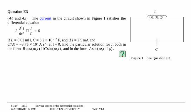
Question E3

(A4 and A5)3The current in the circuit shown in Figure 1 satisfies thedifferential equation

Ld2 I

dt2+ I

C= 0

If L = 0.021mH, C = 3.2 × 100−101F, and if I = 2.51mA and

dI/dt = −3.75 × 1041A s−1 at t = 0, find the particular solution for I, both in

the form Bcos(ω0t) + C sin (ω0t) , and in the form Asin (ω0t + φ ) .


Question E4

(A2, A4 and A6)3In a certain medium, the z-component of the electric field, Ez, varies with x, the distance fromthe boundary of the medium, according to the equation

d2Ez

dx2+ Ω 2

c2Ez − µ 2Ez = 0

where Ω, c and µ are positive constants. Find the general solution to this equation in the three cases:

(a) Ω > µc, (b) Ω = µc, (c) Ω < µc.


L

CR

Figure 53A circuit containing aninductance L, a resistor R and acapacitor C, connected in series.

Question E5

(A7)3In the circuit shown in Figure 5, L has the value 0.021mH and C hasthe value 3.2 × 10−10

1F. The current in the circuit satisfies Equation 28.

Ld2 I

dt2+ R

dI

dt+ I

C= 0 (Eqn 28)

For what values of R will the current display lightly damped, oscillatorybehaviour?

Find the general solution to Equation 28 (a) if R = 3001Ω, (b) if R = 13001Ω,(c) if R = 5001Ω.


Question E6

(A8 and A9)3(a) Explain what is meant by the term complementary function.

(b) Find the general solution to the differential equation:

d2 y

dt2+ ω0

2 y = A cos(Ω t)

where ω, A, Ω are constants and Ω12 ≠ ω02.

Study comment This is the final Exit test question. When you have completed the Exit test go back to Subsection 1.2 andtry the Fast track questions if you have not already done so.

If you have completed both the Fast track questions and the Exit test, then you have finished the module and may leave ithere.

flexible learning approach to physics ÊÊÊ module m6.3 ... … · flap m6.3 solving second-order...

Documents