Flexible Policy Construction by Information Refinement 315

Flexible Policy Construction by Information Refinement

Michael C. Horsch horsch@cs.ubc.ca

David Poole poole@cs.ubc.ca

Department of Computer Science University of British Columbia

2366 Main Mall, Vancouver, B.C., Canada V6T 1Z4

Abstract

We report on work towards flexible algorithms for solving decision problems represented as in­fluence diagrams. An algorithm is given to con­struct a tree structure for each decision node in an influence diagram. Each tree represents a decision function and is constructed incremen­tally. The improvements to the tree converge to the optimal decision function (neglecting com­putational costs) and the asymptotic behaviour is only a constant factor worse than dynamic programming techniques, counting the number of Bayesian network queries. Empirical results show how expected utility increases with the size of the tree and the number of Bayesian net calcu­lations.

1 INTRODUCTION

Influence diagrams provide expressive and intuitive rep­resentations for an important class of decision problems [Howard and Matheson, 1981; Shachter, 1986; Pearl, 1988]. Small problems can be solved by finding a pol­icy which maximizes the decision maker's expected util­ity without considering the cost of computation, but finding such a policy requires an exponential number of maximiza­tions, in terms of the number of decisions in the problem [Shachter, 1986; Shachter and Peot, 1992; Zhang, 1994; Cooper, 1990].

When the costs of computation are taken into account, the decision maker must be concerned not only about the out­comes of acting in the world, but also about effects of com­puting on finite hardware while other processes in the world continue [Horvitz, 1990; Russell and Wefald, 1992].

We report a technique to compute policies for decision problems expressed as influence diagrams. For each deci­sion node in the influence diagram, the technique builds a decision function in the form of a tree whose non-leaf ver­tices are labelled with predecessors of the decision node, and whose leaf vertices are labelled with actions.

For each decision node in an influence diagram, our tech­nique iteratively refines the information contained in the tree. The tree starts as a single leaf, representing an ac­tion to be carried out regardless of the available informa­tion. The incremental improvement replaces a leaf, i.e., an action taken based on a certain subset of information, with a vertex, i.e., a variable which is observable to the decision maker. New leaves are added, representing actions to be taken given the distinctions made in the path from root to leaf in the tree.

The decision function can be refined in this way until some stopping criterion is met, or until there are no more observ­able variables to add to the tree. A tree which cannot be fur­ther refined can represent the same "optimal" decision func­tion that would be computed by traditional dynamic pro­gramming techniques.

For a decision node with n informational predecessors, each having at most b values, the sequence of improvements to a tree ends after O(bn) queries to a Bayesian network [Shachter and Peot, 1992], and is a constant factor worse than traditional dynamic programming techniques. How­ever, our technique is not intended for finding optimal poli­cies; the advantage of our technique is that a policy is avail­able immediately, and it is improved incrementally with fur­ther computation.

This technique is a step towards flexible iterative refinement of policies for decision problems [Horvitz, 1990]: decision functions are available in an anytime manner, with an non­decreasing expected value as more computational resources are devoted to the problem and the next iteration in the se­quence is performed by refining the previous policy. Each tree in the sequence represents a sub-optimal decision func­tion, whose expected value to the decision maker is well de­fined.

Our empirical results suggest that small trees can be com­puted before an optimal decision function, and while they are sub-optimal, they have positive value for a decision maker reasoning with bounded resources.

316 Horsch and Poole

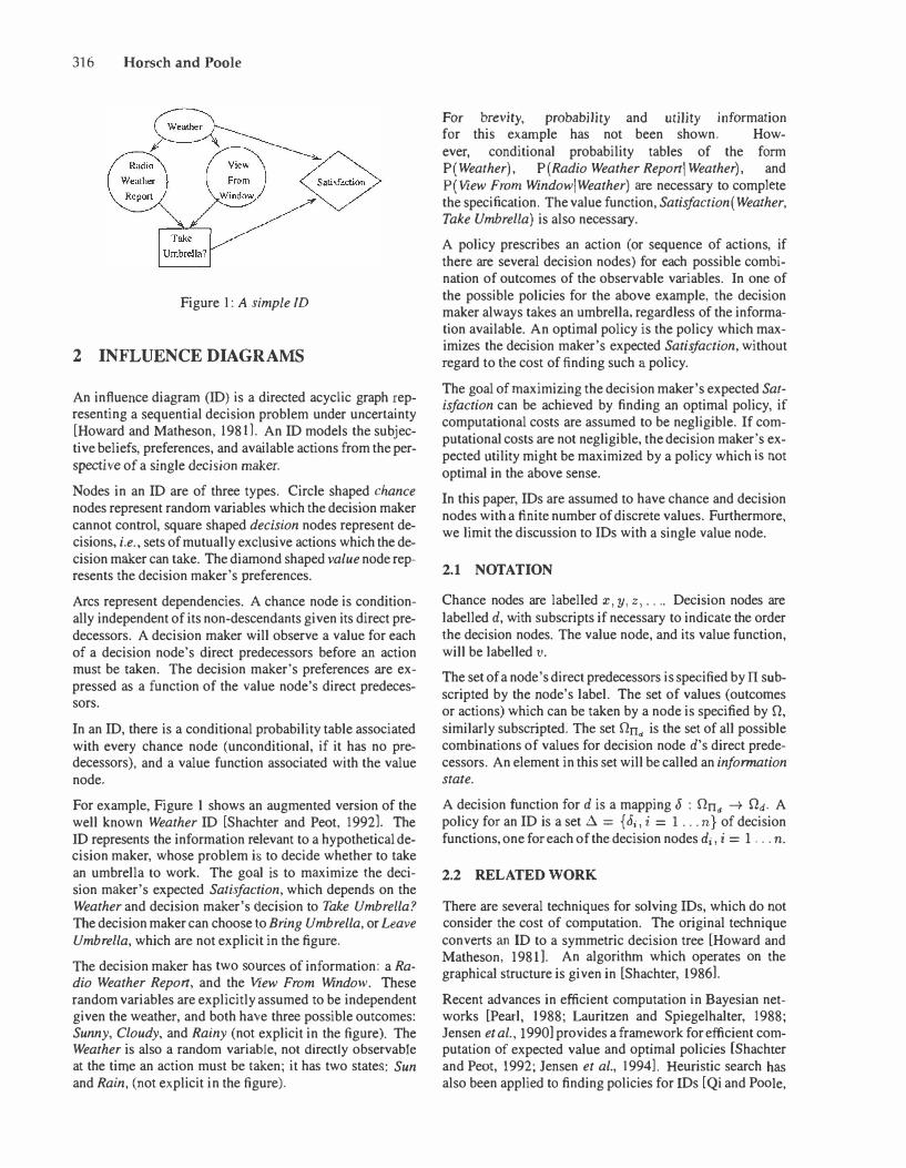
Figure 1: A simple ID

2 INFLUENCE DIAGRAMS

An influence diagram (ID) is a directed acyclic graph rep­resenting a sequential decisi{)n problem under uncertainty [Howard and Matheson, 1980. An ID models the subjec­tive beliefs, preferences, and available actions from the per­spective of a single decision maker.

Nodes in an ID are of three types. Circle shaped chance nodes represent random variables which the decision maker cannot control, square shaped decision nodes represent de­cisions, i.e. , sets of mutually exclusive actions which the de­cision maker can take. The diamond shaped value node rep­resents the decision maker's preferences.

Arcs represent dependencies. A chance node is condition­ally independent of its non-descendants given its direct pre­decessors. A decision maker will observe a value for each of a decision node's direct predecessors before an action must be taken. The decision maker's preferences are ex­pressed as a function of the value node's direct predeces­sors.

In an ID, there is a conditional probability table associated with every chance node (unconditional, if it has no pre­decessors), and a value function associated with the value node.

For example, Figure 1 shows an augmented version of the well known Weather ID [Shachter and Peat, 19921 The ID represents the information relevant to a hypothetical de­cision maker, whose problem is to decide whether to take an umbrella to work. The goal is to maximize the deci­sion maker's expected Satisfaction, which depends on the Weather and decision maker's decision to Take Umbrella? The decision maker can choose to Bring Umbrella, or Leave Umbrella, which are not explicit in the figure.

The decision maker has two sources of information: a Ra­dio Weather Report, and the View From Window. These random variables are explicitly assumed to be independent given the weather, and both have three possible outcomes: Sunny, Cloudy, and Rainy (not explicit in the figure). The Weather is also a random variable, not directly observable at the time an action must be taken; it has two states: Sun and Rain, (not explicit in the figure).

For brevity, probability and utility information for this example has not been shown. How­ever, conditional probability tables of the form P(Weather), P(Radio Weather Report! Weather), and P(View From Window! Weather) are necessary to complete the specification. The value function, Satisfaction( Weather, Take Umbrella) is also necessary.

A policy prescribes an action (or sequence of actions, if there are several decision nodes) for each possible combi­nation of outcomes of the observable variables. In one of the possible policies for the above example, the decision maker always takes an umbrella, regardless of the informa­tion available. An optimal policy is the policy which max­imizes the decision maker's expected Satisfaction, without regard to the cost of finding such a policy.

The goal of maximizing the decision maker's expected Sat­isfaction can be achieved by finding an optimal policy, if computational costs are assumed to be negligible. If com­putational costs are not negligible, the decision maker's ex­pected utility might be maximized by a policy which is not optimal in the above sense.

In this paper, IDs are assumed to have chance and decision nodes with a finite number of discrete values. Furthermore, we limit the discussion to IDs with a single value node.

2.1 NOTATION

Chance nodes are labelled x, y 1 z 1 • • •• Decision nodes are labelled d, with subscripts if necessary to indicate the order the decision nodes. The value node, and its value function, will be labelled v.

The set of a node's direct predecessors is specified by II sub­scripted by the node's label. The set of values (outcomes or actions) which can be taken by a node is specified by n, similarly subscripted. The set !Jnd is the set of all possible combinations of values for decision node d's direct prede­cessors. An element in this set will be called an information state.

A decision function ford is a mappingS : !Jnd --+ Od. A policy for an ID is a set � = { S;, i = 1 . . . n} of decision functions, one for each of the decision nodes d;, i = 1 . . . n.

2.2 RELATED WORK

There are several techniques for solving IDs, which do not consider the cost of computation. The original technique converts an ID to a symmetric decision tree [Howard and Matheson, 198ll An algorithm which operates on the graphical structure is given in [Shachter, 19861.

Recent advances in efficient computation in Bayesian net­works [Pearl, 1988; Lauritzen and Spiegelhalter, 1988; Jensen et al., 1990] provides a framework for efficient com­putation of expected value and optimal policies [Shachter and Peat, 1992; Jensen et al., 1994]. Heuristic search has also been applied to finding policies for IDs [Qi and Poole,

Flexible Policy Construction by Information Refinement 317

1995] using these advances. We use Bayesian networks (BNs) as the underlying computational engine for our tech­nique to compute posterior probabilities and expected val­ues [Shachter and Peot, 1992].

A number of researchers have described iterative ap­proaches to solving influence diagrams. Beckerman et al., [ 1989] and Lehner and Sadigh [ 1993] use tree structures to represent policies, and use a greedy approach to incremen­tal improvement of the tree structure. Both approaches use a single tree to represent the policy. Lehner and Sadigh de­fine optimality of a decision tree with respect to the number of nodes in the tree, and give a general property which guar­antees that an optimal decision tree of a certain size can be found by greedy search. Beckerman et al. weigh the value of the tree against the cost of computing it, but the tree itself is intended as an alternative to on-line decision making.

Our work extends the previous work by building a deci­sion function, in the form of a tree, for each decision node, taking advantage of efficient probabilistic inference tech­niques. This combination creates a basis for on-line, re­source bounded computation.

3 SINGLE STAGE COMPUTATIONS

We use trees to represent decision functions. In this sec­tion we show how these trees can be built. We call the trees "decision trees" because of the relationship to the ma­chine learning literature (e.g., [Quinlan, 1986]). The reader should be aware that our decision trees differ from the oper­ations research decision trees in that our decision trees are used to represent solutions (or partial solutions) to decision problems, whereas operations research decision trees repre­sent a decision problem. However, the two have much sim­ilarity in structure, which seems sufficient reason to use a common name; the difference in their respective uses seems sufficient to prevent confusion.

In this section, we consider the case where the decision problem has a single decision node, and extend the idea to IDs with multiple decision nodes in Section 4.

3-1 DECISION TREES

Let d be a decision node in an ID. A decision tree t for d is either a leaf labelled by an action dj E Od or a non-leaf node labelled with some observable variable x E Tid. Each non-leaf has a child decision tree for every value Xi<; E Ox. An information predecessor X E rrd appears at most once in any path from the root to a leaf. Each vertex v has a context, lv, defined to be the conjunction of variable assignments on the path from the root of the tree to v. The action at the leaf represents the action to be taken in the context of the leaf. Given an information state w E Orrd, there is a correspond­ing path through a decision tree for d, starting at the root leading to a leaf, which is labelled with the prescribed ac­tion for w. Note that the context of an action need not con­tain every variable in rrd.

View from Window

Leave Umbrella Radio Weather report Take Umbrella

Sunn Rainy

Cloud

Leave Umbrella Leave Umbrella Take Umbrella

Figure 2: A decision tree representation of a policy for the ID in Figure 1.

A decision tree represents a decision function. We will refer to the action prescribed by a decision function by <5 ( w) for information state w, or by dl if l is a leaf on a given decision tree.

A decision tree is shown in Figure 2. The tree can be in­terpreted as a policy for the 10 in Figure 1 as follows. The decision maker first considers the view from the window. If the view is cloudy, then the decision maker will determine what to do by consulting the radio weather report. However, if the view from the window is sunny or rainy, then the radio report need not be consulted at all, even though the report is available as information. Note that in this example, the decision tree represents a policy. In general, we will con­struct a decision tree for each decision node in an influence diagram (Section 4).

We define expected value of a decision tree, so that we can compare decision trees, as follows:

Et = L u(d,l!z)P(it) lEt

where u( dl7) is the expected value of an action din a con­text 7, and the summation is over all leaves in t.

The optimal decision tree is defined as the one whose ex­pected value is greater or equal to the expected value of any other decision tree: t is optimal if for all t', Et � Et'· This definition of optimal does not take into account the cost of computation.

3.2 THE SINGLE STAGE ALGORITHM

We build decision trees using a technique which resembles decision tree learning methods (e.g., [Quinlan, 1986]).

For a given leaf l in a decision tree, its context "/I is exten­sible if it does not contain all the observable variables. We refer to the variables which are not in the context as possi­ble extensions, writing��- We will use"' without subscript or argument when we need to refer to an arbitrary context. The symbol 71> represents the empty context, equivalent to the context at the root of a decision tree.

318 Horsch and Poole

A decision tree t can be extended if there is a leaf with an extensible context; otherwise, the tree is called complete. A tree is extended by removing leaf l with context /1, and re­placing it with new vertex x E ��- The issues of choosing a leaf to extend, and choosing a new vertex x are discussed in Sections 3.4 and 3.3, respectively.

The new vertex xis given a new leaf for every value Xj E !:tx, and each leaf will be labelled with an action dj E !:td which maximizes the expected utility in the new context /1 o::::·Xj/1·

The action at a leaf l is chosen on the basis of being the best action for the context 11 :

This action can be determined with one query to a Bayesian network [Shachter and Peot, 1992] (see also Section 3.5). If a vertex has b values, b queries to the BN are required to compute its leaves. Another b queries are needed to com­pute expected value for each leaf.

For a decision tree t, and leaf node l, we define the expected value of improvement, EV It (l, x ) , to be the increase in ex­pected value when t is extended at l with some x E ��, re­sulting in a new tree t':

EV I1(l, x) o:::: Et'- Et

The basic algorithm can be given as follows:

procedure DTl Input:

influence diagram ID with decision node d

Output: a decision tree for d

Start with the tree as a single leaf Do {

Choose a leaf in the tree to extend Replace the leaf with an extension

} Until (stopping criteria are met or tree is complete)

Return the tree

The sequence of trees created by DTl is such that the ex­pected utility of the next tree is never less than that of the previous tree. However, because the procedure is myopic (only a single vertex is added to a context at any time), there is no guarantee that the expected utility will always increase with every extension of the tree. In fact, an ID could be con­structed in which the expected utility of a tree is arbitrarily far from the expected utility of the optimal tree as long as every leaf node is still extensible.

Note also that every decision tree in the sequence can be used by the decision maker at the time a decision must be made. Thus DTl is an any-time algorithm. In this paper, we do not discuss stopping criteria for the algorithm.

The next two sections discuss in detail the issues of choos­ing a leaf to extend (Section 3.4) and choosing an extension for a given leaf (Section 3.3). These two topics are orthog­onal.

3.3 CHOOSING AN EXTENSION FOR A GIVEN LEAF

A given leaf with an extensible context can be extended by choosing an informational variable which is not already in the context In this section we discuss a greedy strategy.

The best extension oft at l is defined as follows:

xi arg maxEV I1(l, x) xEel

arg max L u(dj lxnl )P (xj l11) xH1 Xj€!1..,

This xj represents the greedy improvement to the decision tree. Using this strategy for extending a leaf in DTl results in a procedure we refer to as Greedy-DTl. In the above equation, dj refers to the action which maximizes the de­cision maker's expected utility with respect to the context Xj/1 (as described in the previous section).

Note that EV It only depends on the leaf l, its context 11, and the possible extensions el· Therefore we can look at im­provements to each leaf independently of possible improve­ments to other leaves, a property which we exploit compu­tationally.

By choosing the best of all possible extensions for a given leaf, the Greedy-DTl approach evaluates many extensions which it will never use, with the concomitant queries to the BN. However, the following results give a bound on the number of BN queries.

Theorem 1 Let n be the number of infonnation predeces­sors for a decision node d in an /D. Furthermore, assume that the number of states for any node in the ID is bounded by a constant b. The total number of BN queries made by Greedy-DTl in constructing a complete decision tree ford · l h 2b bn+l ts ess t an (b-l)' .

This follows from the observation that the number of ex­tensions considered by Greedy-DTl at a leaf depends on the size of its context: if decision node d has n predeces­sors, and a leaf has k of these predecessors in its context, then the number of extensions which must be examined to choose the maximum is n- k. If the number of states a pre­decessor can take is bounded by constant b, then during the course of constructing the optimal decision tree, DTl ex­tends bk leaf nodes whose context is of size k. Therefore the total number of extensions considered by Greedy-DTl is

n-1 bn-1 L (n- k)bk-n+I

k=O

Flexible Policy Construction by Information Refinement 319

i=l

i=l

Finally, recall that each extension requires 2b queries to the BN (Section 3.2).

This result implies that Greedy-DTl requires a constant

factor of (b::':p more BN queries than [Shachter and Peot,

1992] to compute the complete tree. We emphasize that its advantage comes from the fact that it is an anytime algo­rithm.

However, choosing the best extension for a given leaf in­curs a significant computational cost for small contexts. In order to heighten the any-time properties of this approach, we have explored the use of random extensions to a given leaf. This strategy, as we will see in Section 5 does not put as much effort into choosing how to extend a given leaf. Section 5 will show how a random approach performs, in comparison to Greedy-DTl.

3.4 CHOOSING A LEAF TO EXTEND

The DTl algorithm does not specify how to choose a leaf to extend. Given the myopic nature of DTl, an obvious strat­egy would be to choose the leaf whose myopic extension would yield the highest increase in EV I. However, the in­Cl .;ase in EV I can only be determined exactly after an ex­tension has been made. Thus some heuristic is necessary to determine which leaf node to extend.

We have explored several strategies, including choosing random leaves, and a post hoc heuristic, described below. These strategies do not make any assumption with respect to the way a particular leaf is extended. That is, the dis­cussion in this section is independent of the issue presented in Section 3.3, where we discussed the best extension for a given leaf.

The effect of the post hoc heuristic is to spend computa­tional effort in contexts where previous effort has provided the best previous results: A leaf is extended based on the in­crease in expected value which was gained when its parent vertex was added to the tree.

Descriptively, suppose a leaf lis to be extended by adding a vertex x. New leaves are generated for x, by choosing ac­tions which maximize expected utility for the new context which now includes x (as described in Section 3.2). The ex­tension brings an increase (possibly zero) in expected value to the tree. Likewise, the parent vertex of every leaf in the tree was added to the tree, increasing the tree's expected value. Of all such vertices, the post hoc heuristic chooses

the one which brought the highest increase, and extends each of its leaves; ties are broken at random.

This heuristic has the advantage of using value information which is already known, as opposed to making an effort to estimate value information. As well, we note that, while the value of past effort doesn't always suggest a good place to make future effort, the incremental nature of DTl will limit the amount of effort spent in any step.

We note that the post hoc heuristic requires a small amount of overhead ordering the most recent extensions to the tree. An alternative, involving less overhead, is to choose a leaf at random.

3.5 IMPLEMENTATION DETAILS

We have implemented the algorithm using two approaches: the Greedy-DTl with the post-hoc heuristic, and a random approach, where leafs are chosen and extended at random. We use a BN to compute expected value, and make some effort to keep the implementation reasonably efficient.

3.5.1 The computational engine

Computation of expected value is based on the conversion of IDs to BNs [Shachter and Peot, 1992]. The utility node is converted to a binary chance node whose conditional prob­ability distribution is the normalized utility function. Deci­sion nodes in the ID are converted to root chance nodes with uniform probability distributions.

The BN derived in this way from an ID is subsequently compiled into a join tree, which can compute posterior probabilities efficiently, using DistributeEvidence and Col­lectEvidence operations [Jensen et al., 1990].

Converting decision nodes to root chance nodes does not af­fect the probability distribution, and makes the size of the largest cliques in the join tree a function of the probabilistic information in the ID. The informational arcs remain part of the ID, but not the underlying BN.

The best action d* E nd to be performed in a state w E flrrd can be found by choosing the action which maximizes the query P(diw, v); the expected value of the best action is computed by querying the utility node P( vlw, d*).

We generalize this result in terms of choosing an action which maximizes expected utility in a given context 'Y (re­call that a context may not include a value for every ob­servable variable in lid)· The corresponding queries are: P( div, /). and P( vld*, 'Y)·

3.5.2 Efficiency issues

We use a priority queue to order the sequence of extensions to a given tree for the post hoc heuristic.

We avoid recomputation by storing the expected value of a leaf, and the expected value of each previous extension in the queue. As well, we store the posterior probability each

320 Horsch and Poole

of non-leaf node given its context. Thus, we need only to compute expected value for a new context; all the remaining information is obtained by look up.

In order to compute EV It ( l, x) , we need to compute the posterior probability P(xj lit(/)). We order the exploration of extensions so that we can enter It (I) as findings once, and query the BN for the posterior probabilities of x E �� on the basis of one DistributeEvidence computation. We still require this computation once for every leaf, but this is in­significant compared to the 2k CollectEvidence computa­tions required to compute the expected value for all k of the leaf's possible extensions.

In our implementation, any leaf node whose context con­tains logical impossibilities (i.e. , the context has probabil­ity zero) is not extended nor is it considered further. Empir­ically, this could have a great effect on the cost of compu­tation and the size of the resulting tree, as shown in the first example in Section 5.

4 MULTISTAGE IDS

In this section, we present our preliminary work on extend­ing the approach to IDs with multiple decision nodes; we will discuss future directions in Section 6.

We apply the DTl algorithm in the traditional dynamic pro­gramming sequence: starting from the last decision in net­work, we compute a decision function, and then proceed backwards to the immediately preceding decision. We al­low the contexts for a given decision tree to contain prede­cessor decision nodes (or not) according to the EV !1•

We note that during the construction of a decision tree for decision node dk, there are decision functions available for decision nodes dk +l , ... , dn, but not for d 1 1 • • • dk _ 1 . The complication is that contexts for dk may not contain actions for all d 1 1 • • • dk -1, and furthermore, the decision functions for dk+l 1 • • • , dn may not contain actions for d1, ... dk.

To deal with this problem of incomplete contexts, we as­sume a uniform probability distribution over any action which is not mentioned in a given context. For an incom­plete context I· the process maximizes expected utility as if the decision maker would act randomly for any decision node not mentioned in 1; the policy, however, would not be stochastic in any sense.

The implementation applies DTl to each decision node in sequence from last to first. When DTl stops working on a particular decision node, the following steps are taken be­fore the process can be applied to the immediately preced­ing decision node. First, some of the informational prede­cessors for the decision node are re-connected to the chance node which represents it using probabilistic arcs; only those predecessors which are used in the decision function are re­connected. A contingency table is then created which is consistent with the decision function, after the manner of [Shachter and Peot, 1992].

Figure 3: The Car Buyer Problem, expressed as an ID.

Note that the anytime properties of our approach are lost when DTl is applied to decision nodes in sequence. This is due to the fact that the sweep back technique builds a pol­icy in a fixed sequence, and once a decision tree is in place for dk, any future extension to dk would invalidate the de­cision trees for decision nodes d 1 , ... , dk _ 1. Therefore, a multistage policy cannot be incrementally improved using the simple sweep back approach.

5 PERFORMANCE

In this section, we demonstrate the empirical behaviour of the Greedy-DTl using the post hoc heuristic. We apply the algorithm to a small well known problem, and a set of larger random problems.

5.1 TERMS OF COMPARISON

We describe the behaviour of an implementation of DTl, running the procedure until the optimal decision tree is achieved. The data points we collect represent decision trees in terms of the tree's expected value, the number of BN computations required to achieve the tree, and the num­ber of interior vertices in the tree. Note that each data point represents a decision function could be used as an anytime solution.

In our examples, value is normalized to [0, 1]. We measure ,the computation cost in terms of the number of BN com­putations required. Recall that each extensible leaf requires 2 ( n - k) + 1 BN computations, where n is the number of predecessors of the decision node, and k is the number of observations in the context of the leaf.

The size of our decision trees is measured in terms of the number of non-leaf vertices in the tree. Assuming binary valued predecessors of a decision node, the number of ac­tions in a tree of size s is s + 1.

We compare our implementation to an hypothetical dy­namic programming algorithm, in which a BN computation is required for every possible observable state [Shachter and

Flexible Policy Construction by Information Refinement 321

0.77

0.76

0.75

� 0.7• -�

l 0.73

� 0.72 ll

! 0.7,

0.7

{).-69

0.68 0

Th• C.r Buye-r Problem

20 40 tiD eo 100 120 u.o 1so 1eo 200 If BN Con'lj)utation:&

Figure 4: The results of using DTl on last decision node of the Car Buyer Problem. The expected value versus the num­ber of BN computations. Each point represents a decision tree, and the rightmost point represents the optimal decision function.

Peot, 1992]. If a decision node in an ID has n binary prede­cessors, then the dynamic programming algorithm requires exactly 2n BN computations to find the optimal decision function containing 2n information states. If required, the expected value of the decision function could be computed with a single BN computation after the decision function has been established. Finally, since the dynamic program­ming algorithm only produces a single solution, it falls un­der the category of inflexible, and for emphasis and brevity, we refer to it as such.

5.2 A CLASSICAL EXAMPLE

To illustrate the behaviour of DTl, we will show its be­haviour on the well-known Car Buyer problem, Figure 3 [Smith et al., 1993]. There are three decision nodes in this problem; in this section, we use DTl to find a decision func­tion for the last decision node.

The ID represents the knowledge relevant to a decision maker deciding whether or not to buy a particular car. The decision maker has the option of performing a number of tests to various components of the car, and the results of these tests will provide information to the decision to buy the car. The actual condition of the car is not observable directly at the time the decision maker must act, but will in­fluence the final value of the possible transaction. A pol­icy for this problem would indicate which tests to do under which circumstances, as well as a prescription to buy the car (or not) given the results of the tests. Due to space con­straints, none ofthe numerical data required to complete the specification of this problem is shown; this information can be found in [Qi and Poole, 1995; Smith et at., 1993]. This problem is well known for its asymmetry; some combina­tions of tests and results are logical impossibilities.

0.765 0 (I • o- <Oo • 0 o) • 0 • • • • • 0 • • • • • • • • • •

0.76

:a- 0.755

� 0.75

! �

0.745

l 0.7•

ilJ 0.735

0.73

0.725

0.72 '-------'-------'----'------'----�----' 0 10 15 20

Siz•ot O.Citlion Tr•• 25

Figure 5: The results of using DTl on last decision node of the Car Buyer Problem. The expected value versus the size of the tree.

Figures 4, 5 and 6 show the performance of DTl on the last decision stage in the problem.

Figure 5 compares the expected value of the decision tree and the size. Again, each point represents a decision tree improved by a single extension. Because of the asymme­tries in the problem, the optimal decision function can be represented with a decision tree with 7 internal vertices and 10 leaves. For this problem, the largest tree computed by DTl has 13 internal vertices and 13 leaves. The inflexible algorithm, unless designed to handle asymmetries (e.g., [Qi and Poole, 1995]), requires a table of 96 entries. The large difference between our trees and the inflexible solution is due to the asymmetries in the problem; our implementation does not extend contexts whose probability is zero.

Figure 4 illustrates the increase in expected value of each decision function, as a function of the number of BN com­putations. The very first decision function for this problem is available after just 2 BN calculations, and has an expected value which is less than 10% from optimal. Each subse­quent point represents an improvement to the decision func­tion by extending the tree by one node. The rightmost point represents the complete decision tree.

For comparison, the inflexible algorithm requires 96 BN computations, to compute a table of 96 actions.

Figure 6 plots expected value versus the computational ef­fort required; essentially, it shows where the work gets done. More work goes into finding the first few trees, as each leaf's context is small, and has many possible exten­sions. Half of the work is done to build a decision tree with 7 internal vertices. As the decision tree gets larger, the num­ber of possible extensions for each context gets smaller. To­wards the end of the process, fewer BN calculations are performed because there are no extensions to the contexts pulled from the queue.

322 Horsch and Poole

200

180

160

140

8 120 i �

! 100

% "' 00 . 60

""

20

0 0

Tne Car Buyer Probl.am

.. ..

..

..

10 iS. ;20 25 Size of Decision Tres

Figure 6: Showing where the work gets done by DTl when computing decision functions for the last decision in the Car Buyer Problem.

5.3 PERFORMANCE ON RANDOM SINGLE DECISION IDS

To show the performance of DTl on a single decision node, we created a number of random influence diagrams with one decision node. Figure 7 illustrates the template ID which we have used to create random decision problems. The template problem has n chance nodes, each of which is an informational predecessor to the decision node. As well, each chance node is a predecessor of the value node. The template can be instantiated by choosing n; random binary probability distributions, i.e., P( Ck), are chosen from a uni­form distribution on ( 0, 1). The utility function is also cho­sen from a uniform distribution (0, 1].

Figure 8, shows the behaviour of DTl on seven instantia­tions with n = 8. Each point in these graphs represents a decision function; there are seven sets of data shown, one point-shape for each ID. Part (a) shows the increase in ex­pected value as the trees increase in size. Part (b) shows the expected value of the decision function as a function of the work done by the algorithm in terms of BN calcula­tions. The right most points represent the optimal decision tree for each problem. The left hand endpoints represent the expected value of the decision tree continuing only a single leaf.

While the data tend to overlap the general trends are clear: expected value increases with the size of the tree, and the work done. The optimal policy can be computed by the in­flexible algorithm in 256 BN computations.

These data illustrate the concern mentioned in Section 3: that the greedy approach produces trees which are small but expensive to compute.

We have two points to make about these graphs. First, even the first few trees will be more valuable to a decision maker than no decision function at all, if there are deadlines or

v

Figure 7: An /D with one decision node and n informational predecessors.

other opportunity costs. Second, the IDs in these graphs are random, and contain no asymmetries due to logical impos­sibilities; there is reason to believe that decision problems faced by real decision makers contain more structure than our random problems do.

We implemented a random DTl, in which a leaf is chosen at random, and extended by choosing a random information variable not in its context; actions are chosen by maximiz­ing expected utility for the randomly selected context. This program was used to find policies for the same random IDs, and Figure 9 plots the expected value versus the number of

BN calculations performed. As before, the rightmost point in each set represents the complete decision tree. Because random DTl only computes extensions it will use, there is a linear relationship between the size of the decision tree and number ofBN calculations. Thus, a graph corresponding to Figure 8(a) is not presented, ·as its shape is identical to Fig­ure 9.

Note that the total amount of work done by the random DTl to complete the tree is less than half of that required by the greedy version. Also note that in the early stages of com­putation, the expected utility of the decision functions com­puted by the two versions are very similar.

5.4 PERFORMANCE ON IDS WITH SEVERAL DECISION NODES

We have applied the Greedy-DTl technique to the Car Buyer problem. These results are preliminary, but encour­aging.

Because the optimal decision tree for the last decision node can be represented with a tree of as few as 7 non-leaf ver­tices, we were able to explore the space of all possible deci­sion trees for the three decision nodes. Note that the first de­cision node has no informational predecessors, and the sec­ond has two.

The sweep back method was able to compute the optimal expected value with a total of 33 BN calculations (com­pared to the 113 BN calculations required by the inflexible method). Twenty-nine of these steps were used to find a de­cision function for the last decision node (Buy), which was represented by a tree with a single internal vertex (Result

Flexible Policy Construction by Information Refinement 323

Seven R•ndom 1-1'0$ Seven Randoom 1-IDs 0.75 0.75

0.7 0.7

0.85 i 0.65

� ... l + 0.6 .

� ¥ .?"

{ .ll

0.5

0.45- 0.45 0 32 &4 % 128 160 192 224 0 51� 11i21t ,536 2()48

Siz-e -of Poliey 1 BN Computaijons

(a) (b)

Figure 8: Seven random IDs with 8 informational predecessors each were solved by Greedy-DTl with the post hoc heuris­tic. The improvement of the tree in terms of expected value: (a) as the tree increases in size, and (b) as the number of BN calculations performed increases.

Seven Random 1-lOs 0.75

0.7

! 0.65

� l �

l o.ss

0.5

0.45 0 256 512 768 1024

.If BN Coi'Tl'U'IIItior-..

Figure 9: The same seven random IDs as in Figure 8 each were solved by an implementation of random DT 1. Showing the improvement of the tree in terms of expected value as the number of BN calculations performed increases.

of Test 1), and four leaf vertices. The system was able to use this decision function, and its expected value to deter­mine trivial decision trees for the remaining decision nodes, both represented by a single leaf node (an action to be per­formed regardless of the available information). Together, these three trees represent the optimal policy.

A sub-optimal policy, in which the deCision maker decides to make no tests and buy the car is found with 6 BN calcula­tions, and the expected value of this policy is about 3% less than the optimal policy's expected value.

6 CONCLUSIONS AND DISCUSSION

We have shown how a decision tree can be constructed iter­atively, and that the iteration converges to the optimal de­cision function. Asymptotically, the number of Bayesian network calculations required by the iterative technique is a constant factor larger than dynamic programming tech­niques.

We have described two dimensions along which the DTl al­gorithm can be varied: which leaf to extend, and how to ex­tend a given leaf. We have presented a greedy approach to extending a leaf, and a post hoc heuristicfor ordering the ex­tensions. The Greedy-DTl with the post hoc heuristic may not be the best use of computational resources, and we are investigating alternatives.

The greedy approach was shown to spend much effort to find the best extension to a given leaf, resulting in trees which are small but expensive to compute. The random ap­proach, where no computational effort at all is made to de­termine how a context should be extended, computed much larger trees with similar computational effort. In the early stages of the process, the two versions produced decision functions whose expected value were similar. The advan­tage of the greedy approach is that when applied to IDs with several decision nodes, a smaller decision tree will recon­nect fewer infonnational arcs, resulting in smaller cliques, and faster BN queries.

There are other possibilities we have not discussed in this paper, including a hyper-greedy approach, in which a leaf is extended by the first extension whose increase in expected value surpasses a given threshold.

324 Horsch and Poole

The post hoc heuristic seems weak. However, its perfor­mance so far has not required us to seek out a better heuris­tic as yet. The choice of heuristic affects the value of the incremental improvement; if the heuristic does not provide a good guess as to the value of the next iteration, only a sin­gle iteration is "1 ost."

The DTl algorithm is an anytime algorithm for IDs with one decision node. Each iteration has a well-defined cost, in terms of the number of BN computations required. An esti­mate of the increase in expected value due to a incremental improvement to the tree would provide the basis for a flex­ible algorithm. Our post hoc heuristic provides a means by which the previous step can be evaluated, but we are inves­tigating this problem further.

We have shown how DTl can be applied to IDs with several decision nodes, in the familiar sweep back technique of dy­namic programming. For IDs with several decision nodes, the anytime property of DTl is lost. We are exploring ways to balance the computational effort across the stages. The dilemma is that the decision maker may need to take ac­tion on the first decision node with some urgency, but all the computational effort could go into finding a decision func­tion for the last decision node.

We have shown preliminary empirical results which are en­couraging: small decision trees have non-trivial value to a decision maker, before inflexible techniques have produced the optimal decision tree. We take this as an encouraging result, especially towards multi-stage IDs. We have con­jectured that the small trees near the end of the decision se­quence provide enough information, in terms of expected value, to allow the decision maker to construct fairly de­tailed decision trees for decisions which must be acted upon chronologically earlier.

Acknowledgements

The authors would like to thank the reviewers for helpful suggestions, and also Brent Boerlage o.f Norsys Software Corp. for advice and support in the use of the Netica API as our Bayesian network engine, and for many discussions. The second author is supported by the Institute for Robotics and Intelligent Systems, Project IC-7, and the National Sci­ences and Engineering Council of Canada Operating Grant OGP0044121 .

References

[Cooper, 1990] G. F. Cooper. The computational com­plexity of probabilistic inference using Bayesian belief networks (research note). Artificial Intelligence, 42(2-3):393-405 , 1990.

[Beckerman et al. , 1989] D. E. Heckerman, John S. Breese, and Eric. J. Horvitz. The compilation of decision models. In Uncertainty in Artificial Intelligence 5, pages 162-1 73, 1989.

[Horvitz, 1 990] Eric J. Horvitz. Computation and action under bounded resources. Technical Report KSL-90-76, Departments of Computer Science and Medicine, Stanford University, 1990.

[Howard and Matheson, 1 98 1 ] R.A. Howard and J.E. Matheson. The Principles and Applications of Decision Analysis. Strategic Decisions Group, CA, 198 1 .

[Jensen et al. , 1990] F. V. Jensen, K.G. Olesen, and S.K. Andersen. An algebra of Bayesian belief universes for knowledge based systems. Networks, 20:637-660, 1 990.

[Jensen et al. , 1994] Frank Jensen, Finn V. Jensen, and Soren L Dittmer. From influence diagrams to junction trees. In Proceedings of the Tenth Conference on Uncer­tainty in Artificial Intelligence, pages 367-373, 1994.

[Lauritzen and Spiegelhalter, 1988] S. L. Lauritzen and D. J. Spiegelhalter. Local computation with probabilities on graphical structures and their application to expert systems. J. R. Statist Soc B, 50(2): 1 57-224, 1 988.

[Lehner and Sadigh, 1993] Paul E. Lehner and Azar Sadigh. Two procedures for compiling influence di-agrams. In Proceedings of the Ninth Conference on Uncertainty in Artificial Intelligence, pages 335-34 1 , 1 993.

[Pearl, 1988] Judea Pearl. Probabilistic Reasoning in In­telligent Systems: Networks of Plausible Reasoning. Mor­gan Kaufmann Publishers, Los Altos, 1988.

[Qi and Poole, 1995] Runping Qi and David Poole. New method for influence diagram evaluation. Computational Intelligence, 1 1 (3):498-528, 1 995.

[Quinlan, 1986] J.R. Quinlan. Induction of decision trees. Machine Learning, 1 :8 1-106, 1 986.

[Russell and Wefald, 1992] Stuart Russell and Eric We­fald. Do the Right Thing: Studies in Limited Rationality. MIT Press, Cambridge, Mass., 1 992.

[Shachter and Peot, 1992] Ross Shachter and Mark Peat. Decision making using probabilistic inference methods. In Proceedings of the Eighth Conference on Uncertainty in Artificial Intelligence, pages 276-283, 1992.

[Shachter, 1986] Ross D. Shachter. Evaluating influence diagrams. Operations Research, 34(6):87 1-882, 1986.

[Smith et al. , 1 993] J. E. Smith, S. Holtzman, and J. E. Matheson. Structuring conditional relationships in influ­ence diagrams. Operations Research, 4 1 :280-297, 1993.

[Zhang, 1994] Nevin Lianwen Zhang. A Computational Theory of Decision Networks. PhD thesis, University of British Columbia, 1994.